J. Chem. Phys. 150, 124101 (2019); https://doi.org/10.1063/1.5088770 150, 124101

© 2019 Author(s).

An extension of the fewest switchessurface hopping algorithm to complexHamiltonians and photophysics inmagnetic fields: Berry curvature and“magnetic” forces

Cite as: J. Chem. Phys. 150, 124101 (2019); https://doi.org/10.1063/1.5088770Submitted: 14 January 2019 . Accepted: 04 March 2019 . Published Online: 25 March 2019

Gaohan Miao, Nicole Bellonzi , and Joseph Subotnik

COLLECTIONS

Note: This paper is part of a JCP Special Topic on Dynamics of Open Quantum Systems.

This paper was selected as an Editor’s Pick

The Journalof Chemical Physics ARTICLE scitation.org/journal/jcp

An extension of the fewest switches surfacehopping algorithm to complex Hamiltoniansand photophysics in magnetic fields:Berry curvature and “magnetic” forces

Cite as: J. Chem. Phys. 150, 124101 (2019); doi: 10.1063/1.5088770Submitted: 14 January 2019 • Accepted: 4 March 2019 •Published Online: 25 March 2019

Gaohan Miao, Nicole Bellonzi, and Joseph Subotnika)

AFFILIATIONSDepartment of Chemistry, University of Pennsylvania, Philadelphia, Pennsylvania 19104, USA

Note: This paper is part of a JCP Special Topic on Dynamics of Open Quantum Systems.a)Electronic mail: subotnik@sas.upenn.edu

ABSTRACTWe present a preliminary extension of the fewest switches surface hopping (FSSH) algorithm to the case of complex Hamiltonians as appro-priate for modeling the dynamics of photoexcited molecules in magnetic fields. We make ansätze for the direction of momentum rescaling,and we account for Berry’s phase effects through “magnetic” forces as applicable in the adiabatic limit. Because Berry’s phase is a nonlocal,topological characteristic of a set of entangled potential energy surfaces, we find that Tully’s local FSSH algorithm can only partially capturethe correct physics.

Published under license by AIP Publishing. https://doi.org/10.1063/1.5088770

I. INTRODUCTION

Fewest switches surface hopping (FSSH)1 has been a verypowerful tool for simulating non-adiabatic dynamics over the lastthirty years.2–6 The basic idea of the FSSH algorithm is to runstochastic dynamics on electronic adiabats, with stochastic switchesbetween adiabats to account for electronic relaxation; in the spiritof Pechukas’s force,7,8 one rescales momenta in the direction of thederivative coupling whenever a hop between surfaces occurs. Thealgorithm has been shown to successfully capture both the short timedynamics of non-adiabatic systems9,10 as well as (their) long timeequilibrium properties.11 At the same time, the cost of FSSH is quitemodest.1,12,13 Of course, Tully’s algorithm has a few well-knownshortcomings: (i) the original algorithm did not treat wave packetseparation correctly, and thus did not model decoherence;14–23

(ii) the algorithm does not treat recoherence correctly;24 and (iii)the algorithm does not include any nuclear quantum effects.25,26

Of the problems above, item (i) has been discussed extensively inthe literature and can largely be corrected; items (ii) and (iii) arelargely intractable with classical, non-interacting trajectories.27,28

Nevertheless, as a testament of the algorithm’s value, FSSH is rou-tinely applied today to simulate non-adiabatic dynamics includingphotochemical processes,4,9,29 scattering,12,30,31 and charge trans-fer in solution.18,32

Interestingly, of all of the applications listed above, there isone glaring omission. To our knowledge, no one has yet usedFSSH to study non-adiabatic dynamics for molecular systems withspin degrees of freedom in strong magnetic fields. More generally,to our knowledge, no one has yet extended the FSSH algorithmto treat complex (rather than real-valued) electronic Hamiltoni-ans. When one considers such an extension, several obvious ques-tions arise, including: (a) How should one incorporate geometricphases semiclassically,33–36 given that a geometric phase is a nonlo-cal, topological property? (b) How should one choose the directionof momentum rescaling when the derivative coupling is complexand there is no unique real vector to isolate? The answers are notobvious.

With this background in mind, the goal of this paper is topropose one possible set of answers and a possible extension ofFSSH to the case of complex Hamiltonians. We will find that our

J. Chem. Phys. 150, 124101 (2019); doi: 10.1063/1.5088770 150, 124101-1

Published under license by AIP Publishing

The Journalof Chemical Physics ARTICLE scitation.org/journal/jcp

current implementation of FSSH behaves reasonably well, thoughone clearly loses some accuracy when moving from the case of realto complex Hamiltonians. In particular, because of topological phaseeffects, we will show that obvious limitations arise for any algorithm(like FSSH) based on independent, spatially local, and time localtrajectories. This paper is structured as follows: In Sec. II, we intro-duce our several ansätze for the FSSH algorithm in the presence ofa complex Hamiltonian. In Sec. III, we make clear our simulationdetails. In Sec. IV, we present our results. In Sec. V, we interpret ournumerical results and give a simple explanation for how geometricphase effects appear in surface hopping, and we propose a generalextension of the FSSH algorithm. Finally, in Secs. VI and VII, wesummarize the paper and present some open questions, respectively.As far as notation is concerned, we use bold characters (e.g., r) todenote vectors and we use plain characters (e.g., H) to denote eitherscalars or operators.

II. METHODSA. Real Hamiltonians

Let us now briefly review the FSSH algorithm. As originallyconceived, the FSSH approach is applicable to the case of real elec-tronic Hamiltonians. Without loss of generality, consider a real two-by-two Hamiltonian (i.e., a Hamiltonian with two electronic states)of the form

H(r) = (V00(r) V01(r)V10(r) V11(r)

). (1)

Here, r is a nuclear coordinate. To simulate semiclassicaldynamics with quantum electronic states and classical nuclei, oneruns an ensemble of independent trajectories, initialized so as tocorrespond to the correct Wigner distribution at time zero.24,37–40

Thereafter, for each trajectory at r, one first diagonalizes H(r) tocompute adiabatic energies E0(r), E1(r) and adiabatic basis |ψ0(r)⟩,|ψ1(r)⟩, and then evolves the trajectory along a single adiabaticsurface, with equations of motion

r =pm

,

p = Fj(r),

ck = −iEk(r)

hck −

1∑l=0

pm⋅ dkl(r)cl (k = 0, 1).

(2)

Here, j is the active surface for a given trajectory. ck is the electronicwavefunction amplitude for the orbital k. Fj(r) ≡ −∇Ej(r) is the adi-abatic force along the surface j, and dkl(r) ≡ ⟨ψk(r)∣∇∣ψl(r)⟩ is thederivative coupling between orbitals k and l.

According to FSSH, trajectories occasionally switch from onesurface to the other. To be specific, Tully proposed1 that a trajectoryon surface 0 switches to surface 1 with rate

g0→1 = max[0,∆tρ11

ρ00]. (3)

Here, ρjk ≡ cjc∗k are density matrix elements, and (c0, c1) is theelectronic wavefunction. Whenever a particle switches surfaces, inorder to conserve energy, one rescales the momentum in the direc-tion of the derivative coupling, d01(r).41 There are many exist-ing references in the literature where one can learn more details

of the FSSH algorithm,1,18,24,42 beginning with Tully’s originalpaper.1

B. Complex HamiltoniansAt this point, we come to the heart of the matter. Consider a

situation whereby a particle with spin interacts with a magnetic fieldand there are two possible electronic states. Because of the magneticfield, the electronic Hamiltonian will no longer be real-valued.43–46

Instead, the electronic Hamiltonian will be complex: V01(r) can haveboth real and imaginary parts,45 and V10(r) = V∗

01(r). For this sit-uation, FSSH is not well defined and two obvious problems presentthemselves.

1. First, note that FSSH depends critically on the existence ofadiabatic states. Now, it is well known that, in the presenceof conical intersections, adiabatic electronic states cannot beglobally defined, even for real electronic Hamiltonians.45 Nev-ertheless, even though FSSH does not account for geometricphase, the algorithm is largely able to model dynamics throughconical intersections, as has been documented in detail pre-viously.47–50 That being said, for the present case of a com-plex Hamiltonian, one must always worry: How should onebest choose the sign of the wavefunctions, when the signhas a true complex phase and not just a plus/minus? And,how should one best incorporate Berry’s phase effects33,51

semiclassically?2. The second obvious question is: What is the (real-valued)

direction for rescaling the momentum? Obviously, Re(d01)is not acceptable as this quantity depends on the choice ofphase for the adiabatic electronic states. Furthermore, for apractical FSSH calculation, we must be able to compute thisdirection using only local information at a single nucleargeometry.

With these two questions in mind, we will propose a few simple androbust extensions of FSSH to complex Hamiltonians.

1. “Magnetic force” ansatzAs far as the changing (Berry) phase of the adiabatic electronic

states, it is well known that the Berry curvature near the crossingregion can be transformed into an effective magnetic field that isapplicable in the adiabatic limit.51,52 Thus, to incorporate Berry’sphase effects into FSSH dynamics, we propose that when a trajec-tory is moving on adiabatic surface j near a crossing point, we willallow each FSSH trajectory to feel this extra “magnetic force”

Fmagj = h

pm× Bj. (4)

Here, Bj is defined to be the Berry curvature33,53

Bj = ∇ × (i⟨ψj∣∇∣ψj⟩) = −i∑k≠j

djk × dkj. (5)

Substituting Eq. (5) into Eq. (4) and utilizing the identity djk = −d∗kj,we find

Fmagj = 2hIm∑

k≠j[djk(

pm⋅ dkj)]. (6)

In the end, for an FSSH simulation moving along adiabat j,we will assume that the “magnetic” force Fmag

j should simply be

J. Chem. Phys. 150, 124101 (2019); doi: 10.1063/1.5088770 150, 124101-2

Published under license by AIP Publishing

The Journalof Chemical Physics ARTICLE scitation.org/journal/jcp

added to the total adiabatic, Born-Oppenheimer force in Eq. (2).Note that p ⋅ Fmag

j = 0 so that this extra “magnetic” force doesnot break energy conservation, but rather turns the direction ofmomentum. Note further that this “magnetic” force disappears forthe case of a real-valued Hamiltonian, where the derivative couplingdjk is real. Interestingly, for a two state problem, Eq. (6) implies thatFmag

0 = −Fmag1 .

2. Direction of momentum rescalingIn order to extend FSSH to the case of a complex Hamiltonian,

we must find an appropriate direction for momentum rescaling, njk,when a hop between adiabats j → k occurs. To be appropriate, thisdirection vector must satisfy at least three constraints: (i) njk mustbe real; (ii) njk should not depend on the phase of the derivative cou-pling djk; (iii) njk must reduce to djk when the complex part of theHamiltonian is removed. Furthermore, we must be able to constructthis direction with only local information at a single nuclear geome-try; we cannot assume that we have any information about a globalreaction coordinate.

With these constraints in mind, the following three ansätze fornjk are possibilities (all of these directions should be normalized tounit vectors):

● Method #1: “Re(d(v ⋅ d))”Because the magnetic force is independent of phase, thefollowing ansatz would appear reasonable:

njk ∝ Re[djk(pm⋅ dkj)]. (7)

Note the strong connection between the magnetic force[Eq. (6)] and njk here: according to Eq. (7), the real partof [djk(

pm ⋅ dkj)] would act as a direction for momentum

rescaling, while the imaginary part acts as a magnetic forcethat modifies motion along a given adiabat [see Eq. (6)].

● Method #2: “Re(eiηd)”Another option for the rescaling direction njk is the real partof the derivative coupling with a robust phase factor. To thisend, one can choose

njk ∝ Re(eiηdjk), (8)

where for every coordinate r, η is chosen so as to maximizethe vector norm ||Re(eiηdjk)||2. Note that, unlike Method#1, this ansatz for η does not depend on any dynamicalproperties of a given trajectory.

● Method #3: “Average d”One last possibility is the averaged derivative coupling(divided by 2i)71

njk ∝12i

(ρjkdkj + ρkjdjk) = Im(ρjkdkj). (9)

Like Method #1, this ansatz depends on the dynamics of agiven trajectory. However, whereas Method #1 makes use ofthe nuclear momentum, Method #3 makes use of the elec-tronic density matrix to construct the rescaling direction.

In practice, as shown in Appendix A, Method #3 performs verypoorly,72 and so below we will focus exclusively on Methods #1and #2.

Throughout this paper, there is one nuance worth reporting.When running FSSH calculations, one needs to choose appropri-ate phases for eigenvectors. To choose these phases, one can useeither (i) eigenvectors computed on the fly, whereby the phase ofa given set of eigenvectors are aligned with the eigenvectors at previ-ous time step by “parallel transport” (i.e., ⟨ψi(t)∣ψi(t + dt)⟩ ≈ 1) or(ii) analytical eigenvectors [see Eq. (12)] for which a global phase isassigned (whenever possible). In our FSSH calculations, we find thatas long as we initialize the system in a consistent fashion, we can useeither phase convention, as the difference between (i) and (ii) is neg-ligible. For the results below, all FSSH data are implemented usingoption (i).

III. SIMULATION DETAILSConsider a simple 2-D system with the following general

Hamiltonian:

H = A⎡⎢⎢⎢⎢⎣

− cos θ(x, y) sin θei�(x,y)

sin θ(x, y)e−i�(x,y) cos θ(x, y)

⎤⎥⎥⎥⎥⎦

. (10)

For a simple model, we define the functions θ(x, y) and �(x, y)to be

θ ≡π2(erf (Bx) + 1),

� ≡ Wy.(11)

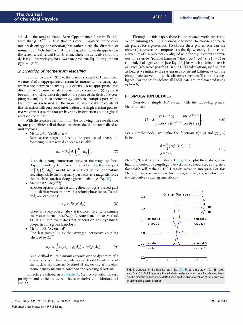
Here A, B, and W are constants. In Fig. 1, we plot the diabats, adia-bats, and derivative couplings. Note that the adiabats are completelyflat which will make all FSSH results easier to interpret. For thisHamiltonian, one may solve for the eigenvalues, eigenvectors, andthe derivative couplings analytically

FIG. 1. Surfaces for the Hamiltonian in Eq. (10). Parameters ar: A = 0.1, B = 3.0,and W = 0.3. Solid lines are the adiabatic surfaces, which are flat; dashed linesare the diabatic surfaces; and dotted lines are the absolute values of the derivativecoupling along each direction.

J. Chem. Phys. 150, 124101 (2019); doi: 10.1063/1.5088770 150, 124101-3

Published under license by AIP Publishing

The Journalof Chemical Physics ARTICLE scitation.org/journal/jcp

E0 = −A,E1 = A,

ψ0 =

⎡⎢⎢⎢⎢⎣

cos θ2 ei�,

− sin θ2

⎤⎥⎥⎥⎥⎦

,

ψ1 =

⎡⎢⎢⎢⎢⎣

sin θ2 ei�,

cos θ2

⎤⎥⎥⎥⎥⎦

,

d00 = i cos2 θ2∇�,

d11 = i sin2 θ2∇�,

d01 =∇θ2

+ i∇�

2sin θ = (

∂xθ2

,i sin θ∂y�

2).

(12)

Note that, with the choice of adiabats in Eq. (12), d01 is composed oftwo components: a real component in the direction of the crossing(∇θ) and an imaginary component in the direction of the gradient ofthe phase of the diabatic coupling (∇�). Vice versa, Berry’s phase isdefined as the integral of the on-diagonal derivative coupling (whichis also called the Berry potential), dkk, around a closed loop C

γk ≡ i∮C⟨ψk∣∇∣ψk⟩ ⋅ dR. (13)

The integral in Eq. (13) is a topological gauge-invariant quantityof much current interest, but for the present paper, we will focusmore on the Berry curvature, i.e., the curl of the Berry potential [seeEq. (5)], which is also gauge invariant.73

For all dynamics reported below, we initialize Gaussian wavepackets on the upper surface incoming from the left,

Ψ0(r) = 0,

Ψ1(r) = eih r⋅pinit e−

∣r−rinit ∣2

σ2 .(14)

Here pinit and rinit are the initial momentum and position, respec-tively; σ is the spread of the initial wave packet over real space.For exact quantum calculations, the wave packets are propagatedwith the Schrödinger equation using the fast Fourier transform tech-nique.54 For the surface hopping algorithm, 107 trajectories are sam-pled from the Wigner distribution corresponding to Eq. (14) (bothr and p are sampled from Gaussian distributions, satisfying ∆ri∆pi= h/2). Each semiclassical trajectory is propagated according to the(modified) FSSH algorithm with an ansatz for the rescaling direc-tion as described above. For a particle moving in the 2-D plane, themagnetic forces are of the following form:

Fmag1 = 2hIm[d10(

pm⋅ d01)] =

h2m

∂xθ∂y� sin θ(−py, px),

Fmag0 =

h2m

∂xθ∂y� sin θ(py,−px).

(15)

For Method #1, the rescaling direction depends on the instantaneousmomentum and is

n01 ∝ ((∂xθ)2px, (∂y� sin θ)2py). (16)

For Method #2, we would ideally like to choose the direction ∇θ,i.e., the x-direction, which we presume is the classical reaction coor-dinate. Unfortunately, with an arbitrary phase possible when delin-eating eigenstates, and without the knowledge of a global potential

energy surface, isolating ∇θ is non-trivial. In the present case (fora general d, see Appendix B), the vector norm f (η) = ||Re(eiηd01)||2

becomes

f (η) =12∣∣Re(eiη

(∇θ + i∇� sin θ))∣∣2. (17)

Maximizing the above expression using ∇θ ⋅ ∇� = 0, Method #2chooses the rescaling direction to be

n01 = {(1, 0) when (∂xθ)2

> (sin θ∂y�)2

(0, 1) when (∂xθ)2< (sin θ∂y�)2. (18)

For most parameters below (except Fig. 7), we will usually oper-ate in the regime whereby (∂xθ)2

> (sin θ∂y�)2, and so n01 willbe in the x-direction. For our other parameters, we choose B = 3.0,rinit = (−3, 0), and σ = 1.0.

IV. RESULTSWe begin by investigating scattering processes where the aver-

age incoming momentum is along the x-direction pinit = (pxinit , 0).

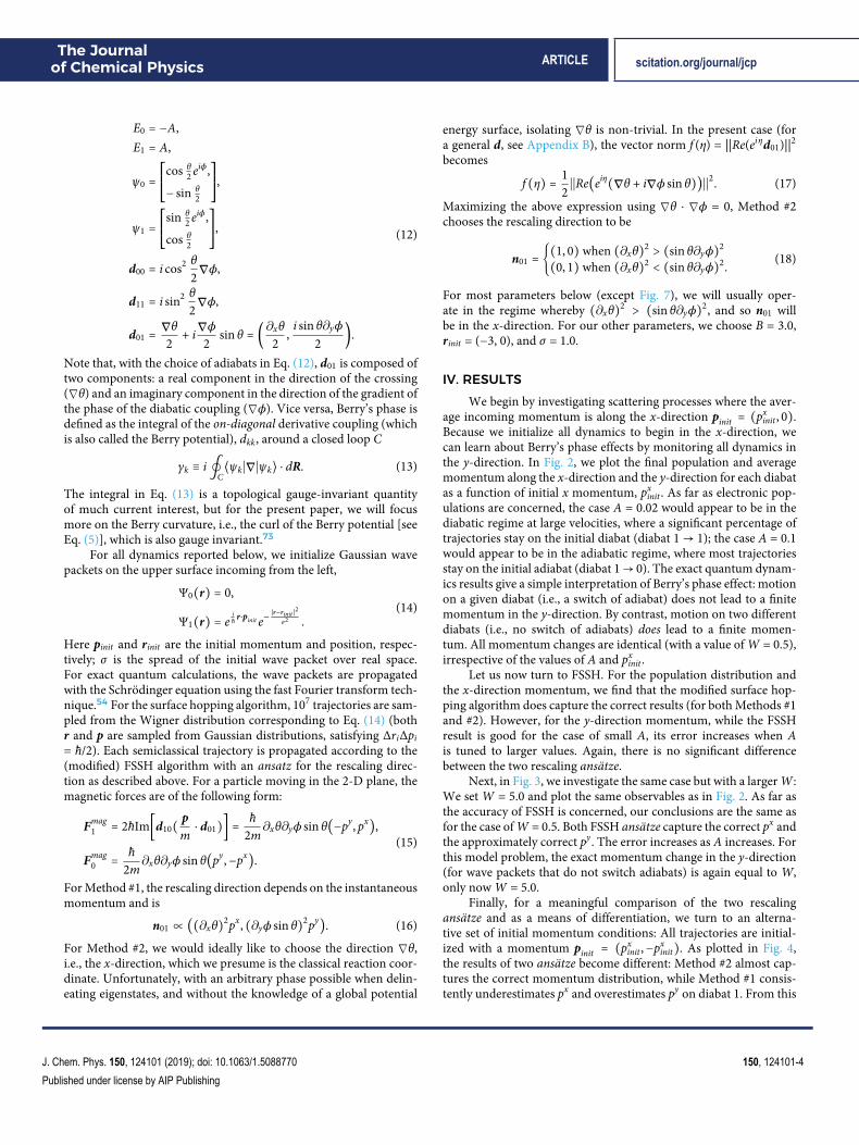
Because we initialize all dynamics to begin in the x-direction, wecan learn about Berry’s phase effects by monitoring all dynamics inthe y-direction. In Fig. 2, we plot the final population and averagemomentum along the x-direction and the y-direction for each diabatas a function of initial x momentum, px

init . As far as electronic pop-ulations are concerned, the case A = 0.02 would appear to be in thediabatic regime at large velocities, where a significant percentage oftrajectories stay on the initial diabat (diabat 1→ 1); the case A = 0.1would appear to be in the adiabatic regime, where most trajectoriesstay on the initial adiabat (diabat 1→ 0). The exact quantum dynam-ics results give a simple interpretation of Berry’s phase effect: motionon a given diabat (i.e., a switch of adiabat) does not lead to a finitemomentum in the y-direction. By contrast, motion on two differentdiabats (i.e., no switch of adiabats) does lead to a finite momen-tum. All momentum changes are identical (with a value of W = 0.5),irrespective of the values of A and px

init .Let us now turn to FSSH. For the population distribution and

the x-direction momentum, we find that the modified surface hop-ping algorithm does capture the correct results (for both Methods #1and #2). However, for the y-direction momentum, while the FSSHresult is good for the case of small A, its error increases when Ais tuned to larger values. Again, there is no significant differencebetween the two rescaling ansätze.

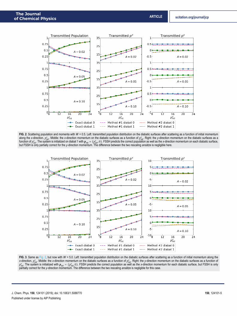
Next, in Fig. 3, we investigate the same case but with a larger W:We set W = 5.0 and plot the same observables as in Fig. 2. As far asthe accuracy of FSSH is concerned, our conclusions are the same asfor the case of W = 0.5. Both FSSH ansätze capture the correct px andthe approximately correct py. The error increases as A increases. Forthis model problem, the exact momentum change in the y-direction(for wave packets that do not switch adiabats) is again equal to W,only now W = 5.0.

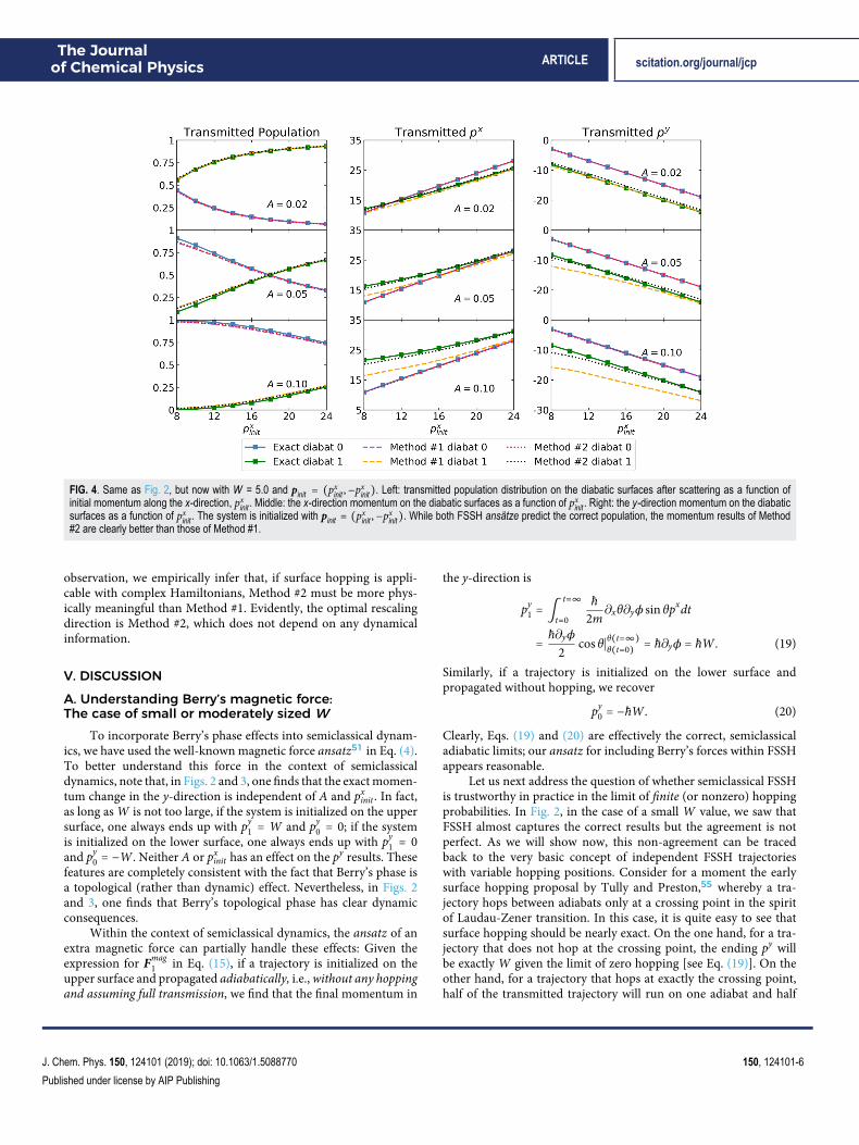
Finally, for a meaningful comparison of the two rescalingansätze and as a means of differentiation, we turn to an alterna-tive set of initial momentum conditions: All trajectories are initial-ized with a momentum pinit = (px

init ,−pxinit). As plotted in Fig. 4,

the results of two ansätze become different: Method #2 almost cap-tures the correct momentum distribution, while Method #1 consis-tently underestimates px and overestimates py on diabat 1. From this

J. Chem. Phys. 150, 124101 (2019); doi: 10.1063/1.5088770 150, 124101-4

Published under license by AIP Publishing

The Journalof Chemical Physics ARTICLE scitation.org/journal/jcp

FIG. 2. Scattering population and momenta with W = 0.5. Left: transmitted population distribution on the diabatic surfaces after scattering as a function of initial momentumalong the x-direction, px

init . Middle: the x-direction momentum on the diabatic surfaces as a function of pxinit . Right: the y-direction momentum on the diabatic surfaces as a

function of pxinit . The system is initialized on diabat 1 with pinit = (p

xinit , 0). FSSH predicts the correct population as well as the x-direction momentum on each diabatic surface,

but FSSH is only partially correct for the y-direction momentum. The difference between the two rescaling ansätze is negligible here.

FIG. 3. Same as Fig. 2, but now with W = 5.0. Left: transmitted population distribution on the diabatic surfaces after scattering as a function of initial momentum along thex-direction, px

init . Middle: the x-direction momentum on the diabatic surfaces as a function of pxinit . Right: the y-direction momentum on the diabatic surfaces as a function of

pxinit . The system is initialized with pinit = (p

xinit , 0). FSSH predicts the correct population as well as the x-direction momentum for each diabatic surface, but FSSH is only

partially correct for the y-direction momentum. The difference between the two rescaling ansätze is negligible for this case.

J. Chem. Phys. 150, 124101 (2019); doi: 10.1063/1.5088770 150, 124101-5

Published under license by AIP Publishing

The Journalof Chemical Physics ARTICLE scitation.org/journal/jcp

FIG. 4. Same as Fig. 2, but now with W = 5.0 and pinit = (pxinit ,−px

init). Left: transmitted population distribution on the diabatic surfaces after scattering as a function ofinitial momentum along the x-direction, px

init . Middle: the x-direction momentum on the diabatic surfaces as a function of pxinit . Right: the y-direction momentum on the diabatic

surfaces as a function of pxinit . The system is initialized with pinit = (p

xinit ,−px

init). While both FSSH ansätze predict the correct population, the momentum results of Method#2 are clearly better than those of Method #1.

observation, we empirically infer that, if surface hopping is appli-cable with complex Hamiltonians, Method #2 must be more phys-ically meaningful than Method #1. Evidently, the optimal rescalingdirection is Method #2, which does not depend on any dynamicalinformation.

V. DISCUSSIONA. Understanding Berry’s magnetic force:The case of small or moderately sized W

To incorporate Berry’s phase effects into semiclassical dynam-ics, we have used the well-known magnetic force ansatz51 in Eq. (4).To better understand this force in the context of semiclassicaldynamics, note that, in Figs. 2 and 3, one finds that the exact momen-tum change in the y-direction is independent of A and px

init . In fact,as long as W is not too large, if the system is initialized on the uppersurface, one always ends up with py

1 = W and py0 = 0; if the system

is initialized on the lower surface, one always ends up with py1 = 0

and py0 = −W. Neither A or px

init has an effect on the py results. Thesefeatures are completely consistent with the fact that Berry’s phase isa topological (rather than dynamic) effect. Nevertheless, in Figs. 2and 3, one finds that Berry’s topological phase has clear dynamicconsequences.

Within the context of semiclassical dynamics, the ansatz of anextra magnetic force can partially handle these effects: Given theexpression for Fmag

1 in Eq. (15), if a trajectory is initialized on theupper surface and propagated adiabatically, i.e., without any hoppingand assuming full transmission, we find that the final momentum in

the y-direction is

py1 = ∫

t=∞

t=0

h2m

∂xθ∂y� sin θpxdt

=h∂y�

2cos θ∣θ(t=∞)θ(t=0) = h∂y� = hW. (19)

Similarly, if a trajectory is initialized on the lower surface andpropagated without hopping, we recover

py0 = −hW. (20)

Clearly, Eqs. (19) and (20) are effectively the correct, semiclassicaladiabatic limits; our ansatz for including Berry’s forces within FSSHappears reasonable.

Let us next address the question of whether semiclassical FSSHis trustworthy in practice in the limit of finite (or nonzero) hoppingprobabilities. In Fig. 2, in the case of a small W value, we saw thatFSSH almost captures the correct results but the agreement is notperfect. As we will show now, this non-agreement can be tracedback to the very basic concept of independent FSSH trajectorieswith variable hopping positions. Consider for a moment the earlysurface hopping proposal by Tully and Preston,55 whereby a tra-jectory hops between adiabats only at a crossing point in the spiritof Laudau-Zener transition. In this case, it is quite easy to see thatsurface hopping should be nearly exact. On the one hand, for a tra-jectory that does not hop at the crossing point, the ending py willbe exactly W given the limit of zero hopping [see Eq. (19)]. On theother hand, for a trajectory that hops at exactly the crossing point,half of the transmitted trajectory will run on one adiabat and half

J. Chem. Phys. 150, 124101 (2019); doi: 10.1063/1.5088770 150, 124101-6

Published under license by AIP Publishing

The Journalof Chemical Physics ARTICLE scitation.org/journal/jcp

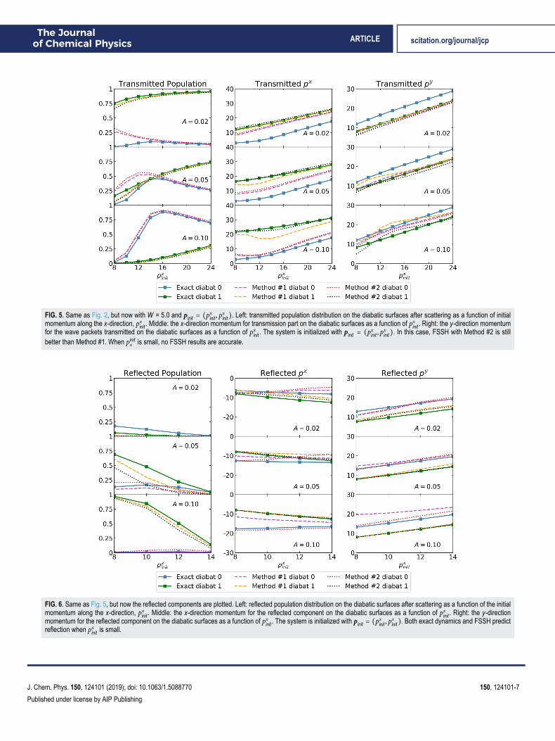
FIG. 5. Same as Fig. 2, but now with W = 5.0 and pinit = (pxinit , px

init). Left: transmitted population distribution on the diabatic surfaces after scattering as a function of initialmomentum along the x-direction, px

init . Middle: the x-direction momentum for transmission part on the diabatic surfaces as a function of pxinit . Right: the y-direction momentum

for the wave packets transmitted on the diabatic surfaces as a function of pxinit . The system is initialized with pinit = (p

xinit , px

init). In this case, FSSH with Method #2 is stillbetter than Method #1. When pinit

x is small, no FSSH results are accurate.

FIG. 6. Same as Fig. 5, but now the reflected components are plotted. Left: reflected population distribution on the diabatic surfaces after scattering as a function of the initialmomentum along the x-direction, px

init . Middle: the x-direction momentum for the reflected component on the diabatic surfaces as a function of pxinit . Right: the y-direction

momentum for the reflected component on the diabatic surfaces as a function of pxinit . The system is initialized with pinit = (p

xinit , px

init). Both exact dynamics and FSSH predictreflection when px

init is small.

J. Chem. Phys. 150, 124101 (2019); doi: 10.1063/1.5088770 150, 124101-7

Published under license by AIP Publishing

The Journalof Chemical Physics ARTICLE scitation.org/journal/jcp

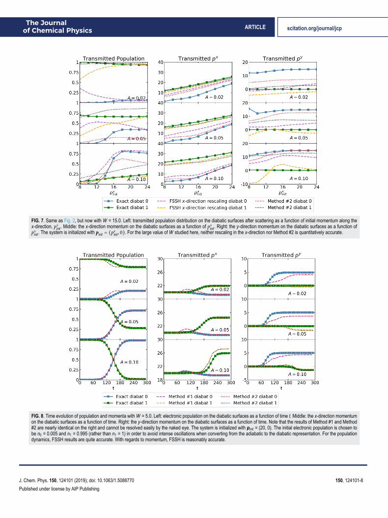
FIG. 7. Same as Fig. 2, but now with W = 15.0. Left: transmitted population distribution on the diabatic surfaces after scattering as a function of initial momentum along thex-direction, px

init . Middle: the x-direction momentum on the diabatic surfaces as a function of pxinit . Right: the y-direction momentum on the diabatic surfaces as a function of

pxinit . The system is initialized with pinit = (p

xinit , 0). For the large value of W studied here, neither rescaling in the x-direction nor Method #2 is quantitatively accurate.

FIG. 8. Time evolution of population and momenta with W = 5.0. Left: electronic population on the diabatic surfaces as a function of time t. Middle: the x-direction momentumon the diabatic surfaces as a function of time. Right: the y-direction momentum on the diabatic surfaces as a function of time. Note that the results of Method #1 and Method#2 are nearly identical on the right and cannot be resolved easily by the naked eye. The system is initialized with pinit = (20, 0). The initial electronic population is chosen tobe n0 = 0.005 and n1 = 0.995 (rather than n1 = 1) in order to avoid intense oscillations when converting from the adiabatic to the diabatic representation. For the populationdynamics, FSSH results are quite accurate. With regards to momentum, FSSH is reasonably accurate.

J. Chem. Phys. 150, 124101 (2019); doi: 10.1063/1.5088770 150, 124101-8

Published under license by AIP Publishing

The Journalof Chemical Physics ARTICLE scitation.org/journal/jcp

will run on the other adiabat. Thus, by symmetry of the Berry’s force,i.e., the fact that Fmag

0 = −Fmag1 , the final py will be 0. Therefore,

Tully-Preston surface hopping must be accurate for incorporatinggeometric phase, and any deviations in the FSSH the py results mustbe caused by the fact that Tully’s FSSH algorithm allows trajectoriesto hop up and down, back and forth, multiple times in the cou-pling region; this complicated hopping picture no longer guaranteesthat the y-momentum induced by the Berry magnetic force will beaccurate. In the end, the small inaccuracies in Figs. 2 and 3 appearinevitable if one sticks with the independent FSSH algorithm, evenin the limit of small W.

B. The limitations of the modified FSSHNext, let us consider larger W values and/or non-perpendicular

incoming velocities (so that Fmag1 is negative in the x-direction),

where another feature can also appear: reflection. Even though theadiabats are entirely flat, it is possible to observe reflection! In Figs. 5and 6, we let py

init = pxinit , and we investigate both the transmitted and

reflected particles, respectively. We find that both the exact quantumsolution and the modified FSSH algorithms predict some amount ofreflection provided that we apply the correct magnetic force in ourFSSH algorithm. That being said, although Method #2 is still bet-ter than Method #1, neither method can fully capture the correctpopulation and momentum quantitatively even when A is small.

Finally, let us address the case of very large W. In Fig. 7, we plotsimulation results for W = 15. For this case, an important nuancearises regarding to our FSSH algorithm. Unlike the case of smallor medium W, where Method #2 is equivalent to rescaling in the

x-direction, for the case of large W, Method #2 can actually rescalemomenta along the x-direction for some coordinates but along they-direction for others [see Eq. (18)]. As a means of assessing thisunusual ansatz, we will introduce yet another rescaling scheme:Simple rescaling along the x-direction after a surface hop.

From the results in Fig. 7, we find that, when W is large, nomodified FSSH algorithm works well.74 One is not even able to cap-ture the electronic state populations as a function of px

init . One canconceive of two possible explanations for this dramatic failure: (i)When W is large, the complex Hamiltonian matrix oscillates rapidlywith frequency W as a function of the coordinate y, and so thedynamics may be outside the classical region, and quantum effectsmay be essential, as in the case of a time-dependent Hamiltonianwith large frequency ω. (ii) It is also possible that we have not yetfound the optimal approach for velocity rescaling after a hop. Under-standing how and why FSSH fails in the case of large W deservesfurther investigation.

C. Time dynamicsBefore concluding, let us turn to time dynamics rather than

scattering probabilities. So far in this manuscript, we have focusedon the asymptotic states after a scattering event—rather than thetime dynamics of the underlying wave function during the scatter-ing event. To better understand the dynamics, in Fig. 8, we plot thetime evolution for the populations and momenta on the diabats. Theinitial momentum pinit is set to be (20, 0). To obtain FSSH statis-tics on the diabatic surfaces, we use method 3 from Ref. 38. Thisconversion method leads to intense oscillations if the wavefunction

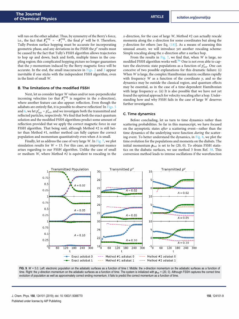
FIG. 9. W = 5.0. Left: electronic population on the adiabatic surfaces as a function of time t. Middle: the x-direction momentum on the adiabatic surfaces as a function oftime. Right: the y-direction momentum on the adiabatic surfaces as a function of time. The system is initialized with pinit = (20, 0). Although FSSH captures the correct timeevolution of population as well as approximately correct ending momentum, it fails to predict the correct momentum as a function of time.

J. Chem. Phys. 150, 124101 (2019); doi: 10.1063/1.5088770 150, 124101-9

Published under license by AIP Publishing

The Journalof Chemical Physics ARTICLE scitation.org/journal/jcp

is initialized entirely on the upper diabatic surface, and to avoid sucha numerical issue, we initialize the wavefunction with a slight super-position state: 99.5% of the population is initialized on the upperdiabatic surface, while 0.5% are initialized on the lower one. Fromthe data in Fig. 8, we find that, despite the fact that the scatteringprocess is dynamically complicated, FSSH dynamics are not actuallythat bad (just as for real Hamiltonians): The population dynamicspredicted by FSSH are reasonably accurate, and the overall trendof momentum dynamics are basically in agreement with the exactdynamics.

Finally, let us turn to the adiabatic representation. To gener-ate exact adiabatic momenta, we rotate the electronic wavefunctionsfrom the diabatic representation to the adiabatic representation,using the analytical eigenvectors in Eq. (12). Note that the quanti-ties ⟨ψ0∣∇∣ψ0⟩ and ⟨ψ1∣∇∣ψ1⟩ are usually non-zero (and of coursepurely imaginary). The contribution of these terms must be includedwhen evaluating the momentum on the adiabatic surfaces. Thus, ifthe exact wavefunction is |Ψ⟩ = C0|ψ0⟩ + C1|ψ1⟩, we estimate theexact momentum on the upper adiabatic surface to be

p1 =⟨C1ψ1∣−ih∇∣C1ψ1⟩

⟨C1ψ1∣C1ψ1⟩

= −ih(C∗1∇C1

C∗1 C1+ ⟨ψ1∣∇∣ψ1⟩). (21)

Next, let us consider FSSH. Normally, because FSSH is definedin the adiabatic basis, one would expect FSSH to be most accuratein this representation. For FSSH, the adiabatic momenta are com-puted simply by averaging the momentum of all trajectories on agiven adiabatic surface.

The dynamics on the adiabatic surfaces are plotted in Fig. 9.For the adiabatic populations, FSSH again captures accurate dynam-ics. For the momentum, however, the FSSH result on adiabat 0 isextremely inaccurate for early times. In theory, this error could arisebecause, at early times, the details of one wave packet spreading fromone adiabat to another must reflect the quantum nature of matterwaves. A simpler and more likely explanation, however, is that FSSHfails here simply because semiclassical dynamics treat p classicallywhereas exact quantum dynamics interprets momentum as a phasechange (that can more naturally account for the presence of geomet-ric phase). Either way, it is quite surprising that physical observables(as calculated by FSSH) in a diabatic basis appear more accurate thanthose in an adiabatic basis.

VI. SUMMARYTo summarize, we have proposed a modified version of

FSSH to incorporate non-adiabatic semiclassical systems with com-plex Hamiltonians. For a chemistry audience accustomed to non-adiabatic transitions, we have shown how to include complex Hamil-tonians and Berry’s forces; for a physics audience accustomed toadiabatic dynamics with complex Hamiltonians, we have shown onemeans to take the non-adiabatic limit and including hopping. Formotion along adiabatic surfaces, we invoke the usual concept of adi-abatic “magnetic forces” to account for Berry’s phase [Eq. (6)], andsome evidence has been provided that this approach is compatiblewith standard FSSH.75,56,57 For the momentum rescaling scheme,we compare three potential ansätze and show that Method #2 is

the best rescaling scheme: after a hop j → k, the momentum shouldbe adjusted in the direction Re(eiηdjk) where η is chosen to maxi-mize ||Re(eiηdjk)||2, which will usually be close to the direction ∇θfor a two-state model (see Appendix B).76 Evidently, choosing adynamical rescaling direction is not appropriate.

With these adjustments, our overall conclusion is that a mod-ified FSSH algorithm can capture many important non-adiabaticdynamical features (e.g., the scattering probabilities and the approx-imate scattering momenta), but FSSH cannot capture a few features(e.g., the detailed early time dynamics of momentum transfer).

VII. OPEN QUESTIONSWith the above summary in mind, several questions now

present themselves. On the practical side, the first methodologi-cal question one must pose is: Have we constructed the optimalFSSH algorithm or is there another, better option available for thecase of a complex electronic Hamiltonian? Considering the errorsin the y-momentum in Figs. 2 and 3 and the discussion of inde-pendent trajectories in Sec. V A, we note that Truhlar et al. haveconstructed an FSSH algorithm with time uncertainty58 which wasdesigned to introduce a small amount of time non-locality. Woulda similar approach help improve FSSH in this case and reduce thenumber of hops in the coupling region? Or is it simply impos-sible to model Berry’s phase well with independent trajectories,given that Berry’s phase is geometric and topological (and thereforeintrinsically non-local)?

Second, again on the practical side, a modern FSSH imple-mentation can avoid calculating derivative couplings unless a hopis required;12 as far as propagating time dependent Schödingerequation, d ⋅ p/m is enough. Unfortunately, in the case of a com-plex Hamiltonian with Berry’s forces, apparently one must calculated at every time step in order to evaluate Fmag

j . One must won-der: is there a practical and efficient approach to construct sucha Berry force easily, ideally a scheme that will be stable with alarge number of electronic states and will avoid the trivial crossingproblem?12,59–63

Third, on the theory side, one must also wonder: can any of ourproposed extensions of FSSH be tied back to a more rigorous theoryof quantum mechanics? For the case of a real electronic Hamilto-nian, our research group and the Kapral research group have suc-cessfully tied FSSH back to the quantum classical Liouville equation(QCLE).39,40 However, the QCLE is a first order expansion that cutsoff at zeroth order in h, whereas Berry’s phase requires a second-order expansion: Note that the magnetic force in Eq. (6) is first orderin h. Can we relate an extended version of FSSH to an extendedversion of the QCLE for the case of complex Hamiltonians?

Fourth, according to Figs. 5 and 6, the magnetic force in Eq. (6)can lead to wave packets separating as trajectories on different adi-abatic surfaces are turned in different directions, some transmittedand some reflected. Thus, the sharp reader will no doubt isolate yetanother question. Recall that, when deriving FSSH from the QCLE,the question of decoherence and wave packet separation arises nat-urally.40 After all, wave packets on different adiabatic surfaces feeldifferent static, adiabatic forces that lead to separation eventually;and for years, many researchers have constructed practical solu-tions for incorporating decoherence into FSSH to account for sucheffects.14,19–23,64–66 For the present paper, however, we now see a

J. Chem. Phys. 150, 124101 (2019); doi: 10.1063/1.5088770 150, 124101-10

Published under license by AIP Publishing

The Journalof Chemical Physics ARTICLE scitation.org/journal/jcp

new phenomenon: With Berry’s forces, wave packet separation iscaused by wave packets on different surfaces feeling different mag-netic forces that depend on velocity. Furthermore, these “magnetic”forces appear only in the strong coupling region, which negatesour usual understanding of decoherence being a phenomenon thatemerges after wave packets pass through coupling region and onlythereafter move apart in different directions.67 Thus, another imme-diate question is how should we appropriately model such magneti-cally induced decoherence within FSSH so as to recover the correctdynamics.

Given the inherent difficulties of including decoherence withinFSSH, the questions above lead to a fifth question: is it possible thata different mixed quantum classical scheme might strongly outper-form FSSH for the case of complex Hamiltonians? In particular, forproblems of decoherence, ab initio multiple spawning (AIMS) is amore natural ansatz.68,69 And yet, AIMS is most efficient in an adi-abatic basis, where single valued wave functions can be difficult tofind. Interestingly, there has been a great deal of work investigat-ing conical intersection’s geometric phase and choice of basis withinAIMS for real Hamiltonians, and the overall conclusion appear tobe that we should run dynamics with electronic wavefunctions cho-sen at a single location.70 Thus, one can ask, can the results inRef. 70 for adiabatic AIMS be easily extended to work with complexHamiltonians?

The final, sixth question is perhaps most exciting of all. On theexperimental front, one must wonder: can any of the dynamics pre-dicted in Sec. IV above be detected experimentally? For instance, thenumerical model above suggests that, whenever an electronic tran-sition (in the x-direction) occurs between two electronic states with

spin, one ought to find a signature of nuclear or vibrational motion(in the y-direction) as arising from Berry’s phase for the case of amolecule in a magnetic field. Can we find realistic molecular systemswith large enough susceptibilities such that, in very large magneticfields, we will observe dynamical Berry phase effects? Or, if we recallthat Marcus theory assumes a threshold amount of nuclear friction,a pessimist must ask: Will the inevitable presence of some nuclearfriction eliminate all such effects? And finally, how will these featuresbehave when the complex phase is more complicated so that ∂y� isnot a constant (as assumed above)? These fascinating experimen-tal and theoretical questions will hopefully be answered in the nearfuture.

ACKNOWLEDGMENTSThis material is based upon work supported by the National

Science Foundation under Grant No. CHE-1764365. J.S. acknowl-edges a David and Lucille Packard Fellowship. J.S. thanks TomoyasuMani, David Yarkony, and Abe Nitzan for insightful discussions.

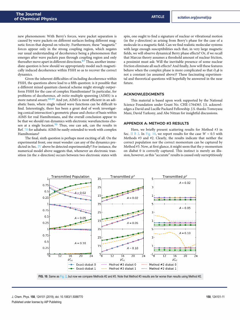
APPENDIX A: METHOD #3 RESULTSHere, we briefly present scattering results for Method #3 in

Sec. II B 2. In Fig. 10, we report results for the case W = 0.5 withMethods #3 and #2. Clearly, the results indicate that neither thecorrect population nor the correct momentum can be captured byMethod #3. Now, at first glance, it might seem that the y-momentumon diabat 0 is correctly captured. This instinct is merely an illu-sion, however, as this “accurate” results is caused only surreptitiously

FIG. 10. Same as Fig. 2, but now we compare Methods #2 and #3. Note that Method #3 results are far worse than results using Method #2.

J. Chem. Phys. 150, 124101 (2019); doi: 10.1063/1.5088770 150, 124101-11

Published under license by AIP Publishing

The Journalof Chemical Physics ARTICLE scitation.org/journal/jcp

from the fact that, at the end of the simulation, the particles remain-ing on the upper adiabatic surface (i.e., diabat 0) are mostly thosetrajectories that never hop, and so the average y-momentum willalways go to the correct answer (as induced by the magnetic force).This correct answer is the zero hopping limit (or adiabatic limit) asdiscussed in Sec. V A that arises from simple classical mechanics(and ignoring all surface hops).

Overall, even though it might appear natural, Method #3 doesnot coincide with the correct physical picture.

APPENDIX B: METHOD #2 WITH A GENERALDERIVATIVE COUPLING

Here, we analyze Method #2 for a general, two-state diabaticproblem. We denote a general (complex) derivative coupling vectoras d ≡ dR + idI . When using Method #2, we maximize the followingwithin the interval η ∈ [0, π)

f (η) = ∣∣Re(eiηd)∣∣2 = ∣∣ cos ηdR − sin ηdI ∣∣2

=12(∣∣dR∣∣

2 + ∣∣dI ∣∣2) +

cos 2η2

(∣∣dR∣∣2− ∣∣dI ∣∣

2) − sin 2ηdR ⋅ dI .

(B1)

Setting f ′(η) = 0 tells us η should satisfy

tan 2η =−2dR ⋅ dI

∣∣dR∣∣2 − ∣∣dI ∣∣2. (B2)

Within the [0, π) interval, there exist two solutions η0 and η1 = η0+ π/2, with η0 ∈ [0, π/2). Using the second derivative f ″(η) < 0, wefind that maximizing f (η) requires that η must satisfy

cos 2η(∣∣dR∣∣2− ∣∣dI ∣∣

2) > 0. (B3)

Thus, for a general d, the solution for η should satisfy both Eqs. (B2)and (B3).

REFERENCES1J. C. Tully, J. Chem. Phys. 93, 1061 (1990).2H. Oberhofer, K. Reuter, and J. Blumberger, Chem. Rev. 117, 10319 (2017).3B. F. Habenicht and O. V. Prezhdo, Phys. Rev. Lett. 100, 197402 (2008).4T. Nelson, S. Fernandez-Alberti, V. Chernyak, A. E. Roitberg, and S. Tretiak,J. Phys. Chem. B 115, 5402 (2011).5F. Sterpone, M. J. Bedard-Hearn, and P. J. Rossky, J. Phys. Chem. A 113, 3427(2009).6T. Nelson, S. Fernandez-Alberti, A. E. Roitberg, and S. Tretiak, Acc. Chem. Res.47, 1155 (2014).7J. C. Tully, Int. J. Quantum Chem. 40, 299 (1991).8P. Pechukas, Phys. Rev. 181, 174 (1969).9B. R. Landry and J. E. Subotnik, J. Chem. Theory Comput. 10, 4253 (2014).10A. Jain and J. E. Subotnik, J. Chem. Phys. 143, 134107 (2015).11P. V. Parandekar and J. C. Tully, J. Chem. Phys. 122, 094102 (2005).12A. Jain, E. Alguire, and J. E. Subotnik, J. Chem. Theory Comput. 12, 5256 (2016).13M. Barbatti, G. Granucci, M. Persico, M. Ruckenbauer, M. Vazdar, M. Eckert-Maksic, and H. Lischka, J. Photochem. Photobiol., A 190, 228 (2007).14B. J. Schwartz, E. R. Bittner, O. V. Prezhdo, and P. J. Rossky, J. Chem. Phys. 104,5942 (1996).15O. V. Prezhdo and P. J. Rossky, J. Chem. Phys. 107, 5863 (1997).16K. F. Wong and P. J. Rossky, J. Chem. Phys. 116, 8418 (2002).17K. F. Wong and P. J. Rossky, J. Chem. Phys. 116, 8429 (2002).18J.-Y. Fang and S. Hammes-Schiffer, J. Chem. Phys. 110, 11166 (1999).

19J.-Y. Fang and S. Hammes-Schiffer, J. Phys. Chem. A 103, 9399 (1999).20M. D. Hack and D. G. Truhlar, J. Chem. Phys. 114, 2894 (2001).21Y. L. Volobuev, M. D. Hack, M. S. Topaler, and D. G. Truhlar, J. Chem. Phys.112, 9716 (2000).22A. W. Jasper and D. G. Truhlar, J. Chem. Phys. 123, 064103 (2005).23O. V. Prezhdo and P. J. Rossky, J. Chem. Phys. 107, 825 (1997).24J. E. Subotnik, A. Jain, B. Landry, A. Petit, W. Ouyang, and N. Bellonzi, Annu.Rev. Phys. Chem. 67, 387 (2016).25I. R. Craig and D. E. Manolopoulos, J. Chem. Phys. 121, 3368 (2004).26S. Jang and G. A. Voth, J. Chem. Phys. 111, 2371 (1999).27A. Donoso and C. C. Martens, Phys. Rev. Lett. 87, 223202 (2001).28A. Donoso, Y. Zheng, and C. C. Martens, J. Chem. Phys. 119, 5010 (2003).29U. Müller and G. Stock, J. Chem. Phys. 107, 6230 (1997).30N. Shenvi, S. Roy, and J. C. Tully, Science 326, 829 (2009).31K. Golibrzuch, P. R. Shirhatti, I. Rahinov, A. Kandratsenka, D. J. Auerbach, A.M. Wodtke, and C. Bartels, J. Chem. Phys. 140, 044701 (2014).32C. A. Schwerdtfeger, A. V. Soudackov, and S. Hammes-Schiffer, J. Chem. Phys.140, 034113 (2014).33M. Berry, Proc. R. Soc. London, Ser. A 392, 45 (1984).34M. Baer, Beyond Born-Oppenheimer: Electronic Nonadiabatic Coupling Termsand Conical Intersections (John Wiley & Sons, 2006).35D. R. Yarkony, Rev. Mod. Phys. 68, 985 (1996).36D. R. Yarkony, J. Phys. Chem. 100, 18612 (1996).37E. Wigner, Phys. Rev. 40, 749 (1932).38B. R. Landry, M. J. Falk, and J. E. Subotnik, J. Chem. Phys. 139, 211101 (2013).39J. E. Subotnik, W. Ouyang, and B. R. Landry, J. Chem. Phys. 139, 214107 (2013).40R. Kapral, Chem. Phys. 481, 77 (2016).41M. F. Herman, J. Chem. Phys. 76, 2949 (1982).42M. Barbatti, Wiley Interdiscip. Rev.: Comput. Mol. Sci. 1, 620 (2011).43C. A. Mead, J. Chem. Phys. 70, 2276 (1979).44S. Yabushita, Z. Zhang, and R. M. Pitzer, J. Phys. Chem. A 103, 5791 (1999).45W. Domcke, D. Yarkony, and H. Köppel, Conical Intersections: ElectronicStructure, Dynamics & Spectroscopy (World Scientific, 2004).46L. T. Belcher, Technical Report AFIT/DS/ENP/11-J01, Air Force Institute ofTechnology, Wright-Patterson AFB OH, School of Engineering and Manage-ment/Department of Engineering Physics, 2011.47I. G. Ryabinkin and A. F. Izmaylov, Phys. Rev. Lett. 111, 220406 (2013).48I. G. Ryabinkin, L. Joubert-Doriol, and A. F. Izmaylov, J. Chem. Phys. 140,214116 (2014).49I. G. Ryabinkin, L. Joubert-Doriol, and A. F. Izmaylov, Acc. Chem. Res. 50, 1785(2017).50R. Gherib, I. G. Ryabinkin, and A. F. Izmaylov, J. Chem. Theory Comput. 11,1375 (2015).51R. Shankar, Principles of Quantum Mechanics (Springer Science & BusinessMedia, 2012).52J. J. Sakurai, J. Napolitano et al., Modern Quantum Mechanics (Pearson, 2014).53C. A. Mead and D. G. Truhlar, J. Chem. Phys. 70, 2284 (1979).54D. Kosloff and R. Kosloff, J. Comput. Phys. 52, 35 (1983).55J. C. Tully and R. K. Preston, J. Chem. Phys. 55, 562 (1971).56M. D. Hack, A. W. Jasper, Y. L. Volobuev, D. W. Schwenke, and D. G. Truhlar,J. Phys. Chem. A 104, 217 (2000).57L. Wang, A. E. Sifain, and O. V. Prezhdo, J. Phys. Chem. Lett. 6, 3827 (2015).58A. W. Jasper, S. N. Stechmann, and D. G. Truhlar, J. Chem. Phys. 116, 5424(2002).59S. Fernandez-Alberti, A. E. Roitberg, T. Nelson, and S. Tretiak, J. Chem. Phys.137, 014512 (2012).60T. Nelson, S. Fernandez-Alberti, A. E. Roitberg, and S. Tretiak, Chem. Phys.Lett. 590, 208 (2013).61F. Plasser, G. Granucci, J. Pittner, M. Barbatti, M. Persico, and H. Lischka, J.Chem. Phys. 137, 22A514 (2012).62L. Wang and O. V. Prezhdo, J. Phys. Chem. Lett. 5, 713 (2014).63G. A. Meek and B. G. Levine, J. Phys. Chem. Lett. 5, 2351 (2014).

J. Chem. Phys. 150, 124101 (2019); doi: 10.1063/1.5088770 150, 124101-12

Published under license by AIP Publishing

The Journalof Chemical Physics ARTICLE scitation.org/journal/jcp

64E. R. Bittner and P. J. Rossky, J. Chem. Phys. 103, 8130 (1995).65J. E. Subotnik and N. Shenvi, J. Chem. Phys. 134, 244114 (2011).66L. Wang, A. Akimov, and O. V. Prezhdo, J. Phys. Chem. Lett. 7, 2100 (2016).67C. Zhu, S. Nangia, A. W. Jasper, and D. G. Truhlar, J. Chem. Phys. 121, 7658(2004).68T. J. Martínez, M. Ben-Nun, and R. D. Levine, J. Phys. Chem. 100, 7884 (1996).69M. Ben-Nun, J. Quenneville, and T. J. Martínez, J. Phys. Chem. A 104, 5161(2000).70G. A. Meek and B. G. Levine, J. Chem. Phys. 145, 184103 (2016).71Of course, njk = Re(ρjkdkj) would be another possibility.72Similarly, njk = Re(ρjkdkj) does not perform well.73Note that, for the case of a real Hamiltonian, where the eigenvectors can alwaysbe chosen as real, Berry’s phase will always be 0 or π. By contrast, for a complexHamiltonian, although the definition of Berry’s phase is identical, the value of thephase itself can now be any number in [0, 2π), as parallel transport along a closedloop with complex wavefunctions can return just about any phase in the end. In

this paper, we will focus mainly on the Berry curvature [see Eq. (5)] rather thanBerry’s phase. Unlike the Berry potential i⟨ψk∣∇∣ψk⟩ (i.e., the integrand of Berry’sphase), the Berry curvature is gauge invariant and has a direct connection to asemiclassical force.74Method #1 also fails (not shown).75Interestingly, we note that, even though FSSH is grounded in the notionof dynamics along adiabats, a few researchers have designed surface hoppingschemes in a diabatic basis.56,57 Within such a diabatic framework, one wouldnot be able to use “adiabatic magnetic forces” to account for Berry’s phase (aswe have done here). Instead, one would need to account for Berry’s phase whenadjusting velocities after a hop, and there is no guarantee that such an approachwould be robust.76Note that, if W is large enough, as discussed in the context of Fig. 7, Method#2 and∇θ may give different rescaling directions. Nevertheless, for such large Wvalues, FSSH does not appear to be accurate—again, see Fig. 7—and so Method#2 would appear to be a robust ansatz that should be applicable for ab initiocalculations.

J. Chem. Phys. 150, 124101 (2019); doi: 10.1063/1.5088770 150, 124101-13

Published under license by AIP Publishing