An Example of Output Regulation for a

Distributed Parameter System with

Infinite Dimensional Exosystem

Christopher I. Byrnes

Systems Science and Math,

One Brookings Dr.

Washington University,

St. Louis, MO 63130

David S. Gilliam

Mathematics and Statistics

Box 41042

Texas Tech University,

Lubbock, TX, 79409-1042

Victor I. Shubov

Mathematics and Statistics

Box 41042

Texas Tech University,

Lubbock, TX, 79409-1042

Jeffrey B. Hood

Department of Mathematics

CRSC

North Carolina State University

Raleigh, NC 27695-8205

Abstract

In this short paper we present an example of the geometric theory of output reg-

ulation applied to solve a tracking problem for a plant consisting of a boundary

controlled distributed parameter system (heat equation on a rectangle) with un-

bounded input and output maps and signal to be tracked generated by an infinite

dimensional exosystem. The exosystem is neutrally stable but with an infinite

(unbounded) set of eigenmodes distributed along the imaginary axis. For this

reason the standard methods of analysis do not apply.

1 Plant and Exosystem

We consider the temperature in a two-dimensional unit square, Ω = [0, 1] × [0, 1], with

coordinates x = (x1, x2) and boundary of Ω denoted by ∂Ω. The temperature distribution

across the region is governed by the Heat Equation. In order to avoid technical difficulties

which do not add any useful information concerning the main point of the paper, we will

arrange for the heat plant to be stable by assuming that some intervals of ∂Ω will have

homogeneous Dirichlet boundary conditions, i.e., the temperature will be held at 0 on those

intervals. This part of the boundary will be denoted by SD, and it will be important that, by

our assumption, SD will consist of a finite union of intervals of positive length. Next, we will

designate another part of the boundary, on which we have Neumann boundary conditions,

by SN = ∂Ω\SD. We designate p non-overlapping input intervals Sj, for j = 1, . . . , p, and p

1

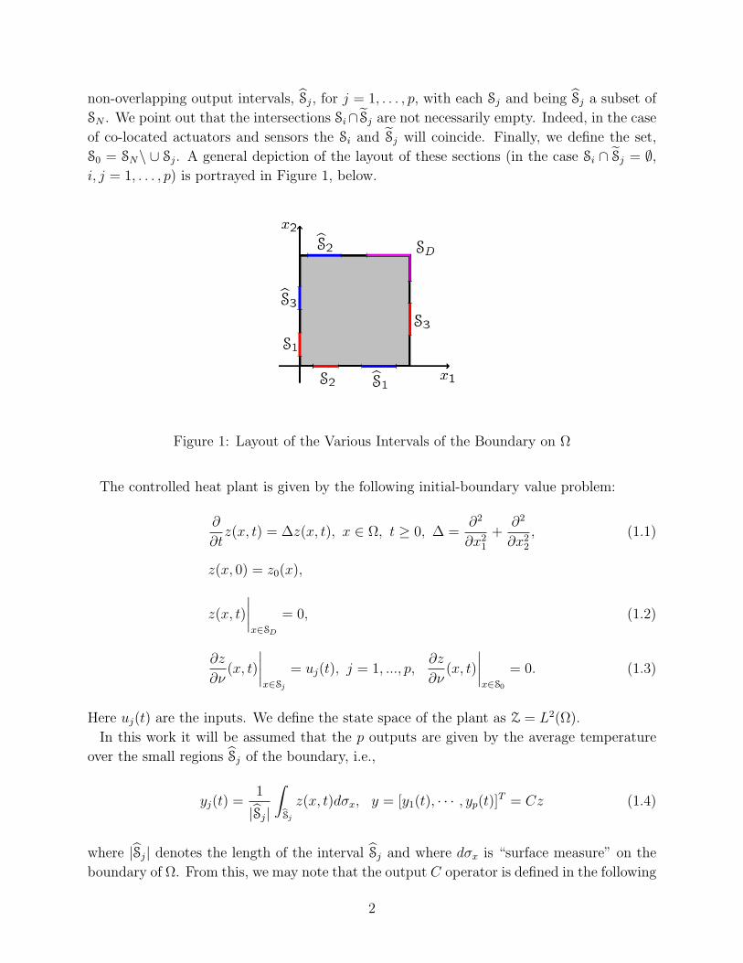
non-overlapping output intervals, Sj, for j = 1, . . . , p, with each Sj and being Sj a subset of

SN . We point out that the intersections Si∩ Sj are not necessarily empty. Indeed, in the case

of co-located actuators and sensors the Si and Sj will coincide. Finally, we define the set,

S0 = SN\ ∪ Sj. A general depiction of the layout of these sections (in the case Si ∩ Sj = ∅,i, j = 1, . . . , p) is portrayed in Figure 1, below.

Figure 1: Layout of the Various Intervals of the Boundary on Ω

The controlled heat plant is given by the following initial-boundary value problem:

∂

∂tz(x, t) = ∆z(x, t), x ∈ Ω, t ≥ 0, ∆ =

∂2

∂x21

+∂2

∂x22

, (1.1)

z(x, 0) = z0(x),

z(x, t)

∣∣∣∣x∈SD

= 0, (1.2)

∂z

∂ν(x, t)

∣∣∣∣x∈Sj

= uj(t), j = 1, ..., p,∂z

∂ν(x, t)

∣∣∣∣x∈S0

= 0. (1.3)

Here uj(t) are the inputs. We define the state space of the plant as Z = L2(Ω).

In this work it will be assumed that the p outputs are given by the average temperature

over the small regions Sj of the boundary, i.e.,

yj(t) =1

|Sj|

∫Sj

z(x, t)dσx, y = [y1(t), · · · , yp(t)]T = Cz (1.4)

where |Sj| denotes the length of the interval Sj and where dσx is “surface measure” on the

boundary of Ω. From this, we may note that the output C operator is defined in the following

2

way

Cz(t) =

1

|S1|

∫S1z(x, t)dσx

...1

|Sp|

∫Spz(x, t)dσx

. (1.5)

Introducing a standard formulation, we write the plant (1.1)-(1.3) in abstract form as

d

dtz = Az +Bu, y(t) = Cz, (1.6)

where A : D(A) ⊂ Z → Z, and C : D(C) ⊂ Z → Y = Rp are unbounded densely defined

linear operators and B : U = Rp → H−1(Ω) where H−α(Ω) denotes the dual of Hα(Ω),

α > 0 (see, e.g., [11]). H−α(Ω) can be identified with a subspace of the space of distributions

H−α(Rn) = [Hα(Rn)]∗ ⊂ D(Rn)∗:

H−α(Ω) =f ∈ H−α(Rn) : supp(f) ⊆ Ω

.

(See definition of B in (1.8)-(1.11) below.)

The operator A = ∆ with domain

D(A) =

ϕ ∈ Z :

∂ϕ

∂ν

∣∣∣∣x∈SN

= 0, ϕ∣∣x∈sSD

= 0

is an unbounded self-adjoint operator in the Hilbert space Z = L2(Ω) whose spectrum

consists of real eigenvalues ζk∞k=1 satisfying

ζk+1 ≤ ζk, ζkk→∞−−−→ −∞, (1.7)

and with associated orthonormal eigenfunctions ϕk(x) satisfying

Aϕk = ζkϕk, 〈ϕn, ϕm〉 = δnm.

(Here and below we denote by 〈·, ·〉 the inner product in L2(Ω)).

The input operator is defined by

Bu(η) =

p∑i=1

ui(t)1

|Si|

∫Si

η(x)dσx, (1.8)

where Bu ∈ H−1(Ω) is a distribution and η ∈ D(Rn) is a test function. Therefore,

Bu =

p∑i=1

uibi, (1.9)

where bi is the distribution which acts on a test function η ∈ D(Rn) by the rule

bi(η) =1

|Si|

∫Si

η(x)dσx, (1.10)

3

and

u =[u1 · · · up

]T ∈ U = Rp. (1.11)

We note that bi ∈ H−1/2−ε(Ω) for ε > 0.

The exosystem is given by the one-dimensional wave equation on the interval [0, 1] (with

spatial coordinate ξ) and with homogeneous Dirichlet boundary conditions.

∂2

∂t2w(ξ, t) =

∂2

∂ξ2w(ξ, t), ξ ∈ (0, 1), t ∈ R (1.12)

w(0, t) = w(1, t) = 0

w(ξ, 0) = ψ0(ξ),∂

∂tw(ξ, 0) = ψ1(ξ). (1.13)

For this exosystem we are interested in reference outputs yrefj (t) given as the displacements

at a set of p points ξp in the interval (0, 1)

yrefj (t) = w(ξj, t), 0 < ξj < 1, yref = Qw =

[yref

1 (t), · · · , yrefp (t)

]T, (1.14)

where Qw would be defined as

Qw =

w(ξ1, t)...

w(ξp, t)

.Once again we recast, in this case the exosystem, as an abstract dynamical system in an

infinite dimensional state space in the usual way by first introducing new dependent variables

W =

[w∂∂tw

]≡

[W1

W2

], W (0) =

[ψ0

ψ1

]≡ W0, S =

0 1∂2

∂ξ20

(1.15)

and then writing the exosystem as:

d

dtW = SW, W (0) = W0 (1.16)

with reference outputs

yref = QW, (1.17)

where

Q =[Q 0

].

The state space for (1.16) is

W = H10 (0, 1)× L2(0, 1),

which is a Hilbert space with inner product defined by⟨[ϕ1

ϕ2

],

[ψ1

ψ2

]⟩W

= 〈ϕ′1, ψ′1〉L2(0,1) + 〈ϕ2, ψ2〉L2(0,1), (1.18)

4

The spectrum of the operator S consists of eigenvalues

λn = nπi, n = ±1,±2, ... (1.19)

and associated normalized eigenfunctions (i.e., ‖Φ`‖W = 1)

Φ` =

1

λ`

1

sin(`πξ), ` = ±1,±2, ...

Thus the exosystem is infinite dimensional with simple eigenvalues along the imaginary axis,

and from (1.7) and (1.19) we note that the respective spectra of A and S are disjoint.

2 Output Regulation Problem

Our objective is to regulate the plant so that its outputs track the reference outputs generated

by the exosystem. To achieve this goal, we follow the program given in [4] and seek u as a

feedback of the state of the exosystem

u = ΓW,

where Γ is a linear map from W to U (= Rp). With this, the plant becomes

d

dtz = Az +BΓW (2.1)

z(0) = z0

and the exosystem given in (1.16) is

d

dtW = SW (2.2)

W (0) = W0.

Now that we have defined the plant and exosystem coupled through the feedback u = ΓW ,

we now define the associated composite system consisting of the inter-connection of these

systems, which will allow us to define the Main Problem and to solve that problem, once

defined. The composite system, is given by

d

dt

[z

W

]=

[A BΓ

0 S

] [z

W

](2.3)

[z

W

](0) =

[z0

W0

].

5

Our tracking problem is formulated in terms of the error, defined as an output of the

composite system given by the difference between the measured output and the reference

output, i.e.,

e(t) = y(t)− yref(t),

where y and yref are defined in (1.4) and (1.17). Written another way,

y = Cz

and

yref = QW,

so that the error can be written in terms of (1.4) and (1.17) as

e(t) = y(t)− yref (t) = [C,−Q]

[z

W

](t). (2.4)

We are now ready to present our main problem.

Problem 2.1 (The Main Problem). Find a feedback control u = ΓW so that for every

initial condition of the plant and exosystem, the error satisfies

e(t) −→ 0 as t −→∞. (2.5)

3 Formal Solution

From the work [3] we know that the open loop system defines a regular linear system [13]

and for any finite dimensional exosystem the following result from [4] provides necessary and

sufficient conditions for the solvability of the associated regulator problem.

Theorem 3.1. The state feedback regulator problem (with finite dimensional exosystem) is

solvable if and only if the regulator equations

ΠS − AΠ = BΓ (3.1)

CΠ−Q = 0 (3.2)

are solvable for bounded linear operators Π : W → D(A) → Z and Γ : W → U.

This result cannot be applied directly to a problem of output regulation with infinite

dimensional exosystem. However, mimicking the proof given in [4] in the present setting we

can obtain formulas which allow us to solve the problem once we introduce an appropriate

modification of the reference signals to be tracked.

We turn to the formal derivation of explicit formulas for Π and Γ solving the regulator

equations (3.1), (3.2). First we note that the first regulator equation (3.1) applied to a

general Φj gives,

ΠSΦj − AΠΦj = BΓΦj

6

and since (λj,Φj) is an eigenpair of S this equation simplifies to

(λjI − A)ΠΦj = BΓΦj. (3.3)

From (1.19) we know that the eigenvalues of S are contained in the resolvent set of A (i.e.,

σ(A) ∩ σ(S) = ∅), which implies that the term (λjI − A) in (3.3) is invertible. This allows

us to solve (3.3) for ΠΦj

ΠΦj = (λjI − A)−1BΓΦj. (3.4)

Applying C to both sides and using (3.2), the second regulator equation, we have

QΦj = C(λjI − A)−1BΓΦj (3.5)

where in (3.5) C(λI − A)−1B is the transfer function of the plant which we denote by

G(λ) = C(λI − A)−1B.

Thus we can rewrite (3.5) as

QΦj = G(λj)ΓΦj.

In order to solve this equation explicitly for ΓΦj, we need to invert G(λj). In this case we

obtain

ΓΦj = G(λj)−1QΦj. (3.6)

Assuming that this can be done for every λj and using the expansion

W =∞∑

j=−∞

〈W,Φj〉Φj, for every W ∈ W,

we can solve, at least formally, (3.6) for u = ΓW in terms of elements we know,

u = ΓW =∞∑

j=−∞

〈W,Φj〉G(λj)−1QΦj. (3.7)

4 Main Technical Difficulties

There are two main difficulties associated with obtaining the formal solution for u = ΓW

given in (3.7):

1. Invertibility of the transfer function G at the eigenvalues of S,

2. Convergence of the resulting infinite sum.

At this point these difficulties have not been fully resolved for the general problems defined

in Sections 2 and 3. To obtain better insight into these problems let us write a formal explicit

expression for the transfer function,

G(λ) = C(λI − A)−1B,

7

given as

G(λ) = C(λI − A)−1B =∞∑

k=1

〈B,ϕk〉Cϕk

λ− ζk, (4.1)

where we recall that B and C are defined in (1.8)-(1.11) and (1.4), (1.5).

Recall that the transmission zeros for a transfer function G(λ) are defined as the set of

complex numbers λ satisfying detG(λ) = 0. As we can see from (3.7) (and is also well known

in the finite dimensional linear case [10]) solvability of the regulator problem requires that the

eigenvalues of S are not transmission zeros of the plant. Unfortunately, it not usually easy

to find the transmission zeros explicitly although there has been some work in this direction.

For example, in the SISO case it has been shown in [12] in special cases the transmission

zeros are real and interlace with the negative eigenvalues. In the SISO case with co-located

actuators and sensors (i.e., when the input regions and output regions are the same, Sj = Sj,

for all j), it can be shown that our systems satisfy the necessary conditions to conclude

that no eigenvalue of S is a transmission zero of the transfer function and our first technical

problem is resolved.

Assuming that det(G(λ`)) 6= 0 for all `, for a given problem under consideration, then (at

least formally) as we have seen in (3.7), for any Φ ∈ W, we have

ΓΦ?=

∞∑`=−∞

〈Φ,Φ`〉WG(λ`)−1QΦ`. (4.2)

Unfortunately, it is still not clear that this infinite sum exists.

This brings us to our next fundamental difficulty. Using methods from classical elliptic

boundary value problems, it can be shown that

|G(λ`)| ∼ C1 exp(−C2

√|λ`|)

`→∞−−−→ 0, (4.3)

i.e., the transfer function, evaluated at the eigenvalues λ`, decays exponentially as ` → ∞.

Thus we see that it is extremely difficult for the sum in (4.2) to exist. Indeed, for the sum to

exist 〈Φ,Φ`〉WQΦ` must be rapidly decreasing in order to compensate for the rapid increase

of the terms from G(λ`)−1. From a physical point of view, this corresponds to the well known

fact that a parabolic system does not want to oscillate rapidly so it is difficult for its output

to track a rapidly oscillating output from a hyperbolic system. In order to make the tracking

problem solvable, we must somehow damp high-order oscillations. There are several ways to

deal with this problem. One could truncate high order oscillations by choosing Q so that

QΦ` = 0 for |`| > N, (4.4)

or, equivalently, we could restrict initial data for the exosystem to the span of the eigen-

functions Φ`N`=−N . But this approach really amounts to starting with a finite dimensional

exosystem. Rather than take this approach we change our definiton of the reference signal

8

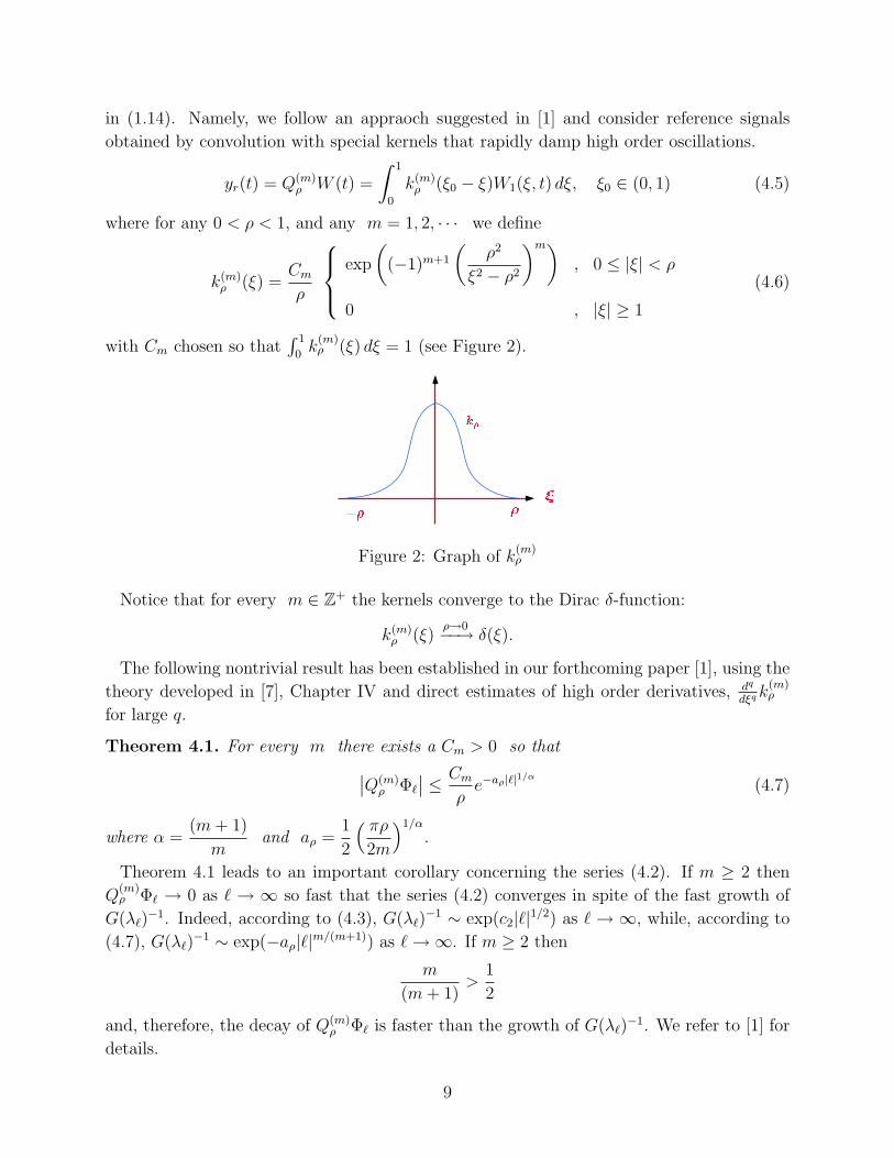
in (1.14). Namely, we follow an appraoch suggested in [1] and consider reference signals

obtained by convolution with special kernels that rapidly damp high order oscillations.

yr(t) = Q(m)ρ W (t) =

∫ 1

0

k(m)ρ (ξ0 − ξ)W1(ξ, t) dξ, ξ0 ∈ (0, 1) (4.5)

where for any 0 < ρ < 1, and any m = 1, 2, · · · we define

k(m)ρ (ξ) =

Cm

ρ

exp

((−1)m+1

(ρ2

ξ2 − ρ2

)m), 0 ≤ |ξ| < ρ

0 , |ξ| ≥ 1

(4.6)

with Cm chosen so that∫ 1

0k

(m)ρ (ξ) dξ = 1 (see Figure 2).

Figure 2: Graph of k(m)ρ

Notice that for every m ∈ Z+ the kernels converge to the Dirac δ-function:

k(m)ρ (ξ)

ρ→0−−→ δ(ξ).

The following nontrivial result has been established in our forthcoming paper [1], using the

theory developed in [7], Chapter IV and direct estimates of high order derivatives, dq

dξq k(m)ρ

for large q.

Theorem 4.1. For every m there exists a Cm > 0 so that∣∣Q(m)ρ Φ`

∣∣ ≤ Cm

ρe−aρ|`|1/α

(4.7)

where α =(m+ 1)

mand aρ =

1

2

( πρ2m

)1/α

.

Theorem 4.1 leads to an important corollary concerning the series (4.2). If m ≥ 2 then

Q(m)ρ Φ` → 0 as ` → ∞ so fast that the series (4.2) converges in spite of the fast growth of

G(λ`)−1. Indeed, according to (4.3), G(λ`)

−1 ∼ exp(c2|`|1/2) as ` → ∞, while, according to

(4.7), G(λ`)−1 ∼ exp(−aρ|`|m/(m+1)) as `→∞. If m ≥ 2 then

m

(m+ 1)>

1

2

and, therefore, the decay of Q(m)ρ Φ` is faster than the growth of G(λ`)

−1. We refer to [1] for

details.

9

5 Numerical Example

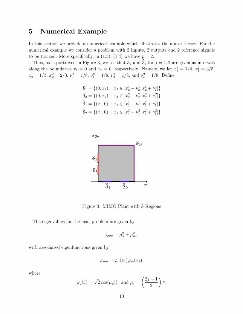
In this section we provide a numerical example which illustrates the above theory. For the

numerical example we consider a problem with 2 inputs, 2 outputs and 2 reference signals

to be tracked. More specifically, in (1.3), (1.4) we have p = 2.

Thus, as is portrayed in Figure 3, we see that Sj and Sj for j = 1, 2 are given as intervals

along the boundaries x1 = 0 and x2 = 0, respectively. Namely, we let x11 = 1/4, x2

1 = 3/5,

x12 = 1/3, x2

2 = 2/3, ν11 = 1/8, ν2

1 = 1/8, ν12 = 1/8, and ν2

2 = 1/8. Define

S1 = (0, x2) : x2 ∈ [x12 − ν1

2 , x12 + ν1

2 ]S2 = (0, x2) : x2 ∈ [x2

2 − ν22 , x

22 + ν2

2 ]

S1 = (x1, 0) : x1 ∈ [x11 − ν1

1 , x11 + ν1

1 ]

S2 = (x1, 0) : x1 ∈ [x21 − ν2

1 , x21 + ν2

1 ]

Figure 3: MIMO Plant with S Regions

The eigenvalues for the heat problem are given by

ζnm = µ2n + µ2

m,

with associated eigenfunctions given by

ϕnm = ϕn(x1)ϕm(x2),

where

ϕj(ξ) =√

2 cos(µjξ), and µj =

(2j − 1

2

)π.

10

Gi,j(λ) = 〈(λI − A)−1bi, cj〉

= 4∞∑

n,m=1

(sin(µmdi)− sin(µmci)

)(sin(µnbj)− sin(µnaj)

)µnµm(bj − aj)(di − ci)(λ− ζnm)

(5.1)

=∑n,m

〈bj, ϕnm〉〈ϕnm, ci〉λ` − ζnm

. (5.2)

For this special case, in the Masters Thesis [8], Jeff Hood has given complete details verifying

that the infinite sum defining G(λ) converges uniformly and absolutely for all λ ∈ ρ(A).

We have chosen an initial condition for the heat equation given by ϕ(x) = x2(1− 2x). For

the exosystem (one dimensional wave equation) we have taken initial conditions

W0 =

[x(1− x)

sin(2x)

].

The representation for the solution to the wave equation

d

dtW = SW, W (0) = W0 =

[ψ0

ψ1

]is given as

W = eStW0 =∞∑

n=−∞

eλnt〈W0,Φn〉WΦn,

or

W =∞∑

n=−∞

eλnt[〈ψ′0,Φ1′

n 〉L2 + 〈ψ1,Φ2n〉L2

]Φn.

From this we obtain the explicit formula for the solution w = W1

w(ξ, t) =√

2∞∑

n=1

[〈ψ0,Ξn〉 cos(nπt) + 〈ψ1,Ξn〉

sin(nπt)

nπ

]sin(nπξ),

where Ξn(ξ) =√

2 sin(nπξ) for n = 1, 2, 3, . . ..

The reference outputs yref are thus approximations to

yr = QW =

[w(ξ1, t)

w(ξ2, t)

]by

yref(t) = Q(2)ρ W (t) =

∞∑`=−∞

eλ`t〈W0,Φ`〉Q(2)ρ Φ`, (5.3)

11

where

Q(2)ρ Φj =

∫ 1

0k

(2)ρ (ξ1 − ξ)Q

(2)ρ Φ`(ξ) dξ∫ 1

0k

(2)ρ (ξ2 − ξ)Q

(2)ρ Φ`(ξ) dξ

.In our numerical example we have set ξ1 = 1/4 and ξ2 = 3/4.

In the numerical simulation we have also truncated the infinite sum and computed

u(t) = ΓW (t) =N∑

`=−N

eλ`t〈W0,Φ`〉G(λ`)−1Q(2)

ρ Φ`, (5.4)

with N = 25.

0

0.5

1

0

2

4

-0.5

0

0.5

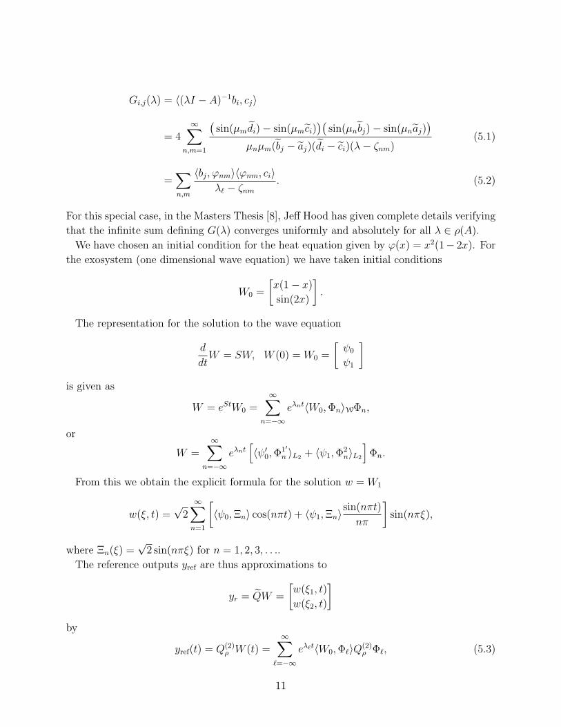
Figure 4: Solution Surface with Output Curves

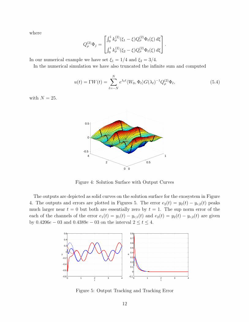
The outputs are depicted as solid curves on the solution surface for the exosystem in Figure

4. The outputs and errors are plotted in Figures 5. The error e2(t) = y2(t) − yr,2(t) peaks

much larger near t = 0 but both are essentially zero by t = 1. The sup norm error of the

each of the channels of the error e1(t) = y1(t) − yr,1(t) and e2(t) = y2(t) − yr,2(t) are given

by 0.4206e− 03 and 0.4389e− 03 on the interval 2 ≤ t ≤ 4.

0 1 2 3 4-0.8

-0.6

-0.4

-0.2

0

0.2

0.4

0.6

t

y

0 1 2 3 4-0.1

0

0.1

0.2

0.3

0.4

0.5

0.6

0.7

0.8

t

e

Figure 5: Output Tracking and Tracking Error

12

The outputs and errors are plotted in Figures 5. The error e2(t) = y2(t) − yr,2(t) peaks

much larger near t = 0 but both are essentially zero by t = 1. The sup norm error of the

each of the channels of the error e1(t) = y1(t) − yr,1(t) and e2(t) = y2(t) − yr,2(t) are given

by 0.4206e− 03 and 0.4389e− 03 on the interval 2 ≤ t ≤ 4.

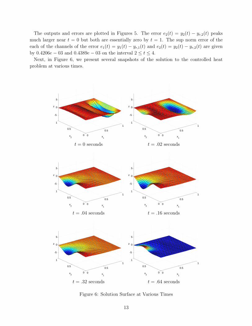
Next, in Figure 6, we present several snapshots of the solution to the controlled heat

problem at various times.

0

0.5

1

0

0.5

1

-5

0

5

x1

x2

z

0

0.5

1

0

0.5

1

-5

0

5

x1

x2

z

t = 0 seconds t = .02 seconds

0

0.5

1

0

0.5

1

-5

0

5

x1

x2

z

0

0.5

1

0

0.5

1

-5

0

5

x1

x2

z

t = .04 seconds t = .16 seconds

0

0.5

1

0

0.5

1

-5

0

5

x1

x2

z

0

0.5

1

0

0.5

1

-5

0

5

x1

x2

z

t = .32 seconds t = .64 seconds

Figure 6: Solution Surface at Various Times

13

References

[1] C.I. Byrnes, J.A. Burns, D.S. Gilliam, V.I. Shubov, Small-scale spatial mollifiers with

efficient spectral filtering properties and output regulation with infinite dimensional

exosystem, preprint Texas Tech University, (2002).

[2] C.I. Byrnes, D.S. Gilliam, I.G. Lauko and V.I. Shubov, “Output regulation for linear

distributed parameter systems,” preprint, 1997.

[3] C.I. Byrnes, D.S. Gilliam, V.I. Shubov, G. Weiss, “Regular Linear Systems Governed

by a Boundary Controlled Heat Equation,” to appear in Journal of Dynamical and

Control Systems.

[4] C.I. Byrnes, D.S. Gilliam, J.B. Hood, and V.I. Shubov, “Output regulation for Regular

Linear Systems,” Preprint TTU, 2002.

[5] C.I. Byrnes and A. Isidori, “Output regulation of nonlinear systems,” IEEE Trans.

Aut. Control 35 (1990), 131-140.

[6] R.F. Curtain and H.J. Zwart, An Introduction to Infinite-Dimensional Linear Systems,

Springer-Verlag, New York, 1995.

[7] I.M. Gel’fand and G.E. Shilov “Generalized Functions, Volume 2” Spaces of funda-

mental and generalized Functions,” Academic Press Inc. 1968.

[8] J.B. Hood, “Output Regulation for a Boundary Controlled Two-dimensional Heat

Equation,” Masters Thesis, Texas tech University, 2002.

[9] J.L. Lions and E. Magenes, Nonhomogeneous Boundary Value Problems & Applica-

tions, Springer-Verlag, New York, 1972.

[10] H.W. Knobloch, A. Isidori, and D. Flockerzi, “Topics in Control Theory,” DMV Sem-

inar Band 22, Birkhauser, 1993.

[11] V.I. Shubov, An Introduction to Sobolev Spaces and Distributions, Lecture Notes, Texas

Tech University, 1996.

[12] H.J. Zwart and M.B. Hof, “Zeros of Infinite-Dimensional Systems,” preprint, University

of Twente.

[13] G. Weiss, “Regular linear systems with feedback,” Math. of Control, Signals and Sys-

tems 7 (1994), 23-57.

14