Embed Size (px)
Citation preview
Modeling, estimation and control of distributed parameter systems:application to transportation networks
by
Sebastien Blandin
A dissertation submitted in partial satisfaction of the
requirements for the degree of
Doctor of Philosophy
in
Engineering – Civil and Environmental Engineering
in the
Graduate Division
of the
University of California, Berkeley
Committee in charge:Professor Alexandre M. Bayen, Chair
Professor Laurent El GhaouiProfessor Lawrence C. EvansProfessor Sanjay GovindjeeProfessor Roberto Horowitz
Professor Alexander Skabardonis
Spring 2012
Modeling, estimation and control of distributed parameter systems:application to transportation networks
Copyright 2012by
Sebastien Blandin
1
Abstract
Modeling, estimation and control of distributed parameter systems:application to transportation networks
by
Sebastien BlandinDoctor of Philosophy in Engineering – Civil and Environmental Engineering
University of California, Berkeley
Professor Alexandre M. Bayen, Chair
The research presented in this dissertation is motivated by the need for well-posed math-ematical models of traffic flow for data assimilation of measurements from heterogeneoussensors and flow control on the road network.
A new 2×2 partial differential equation (PDE) model of traffic with phase transitions isproposed. The system of PDEs constitutes an extension to the Lighthill-Whitham-Richardsmodel accounting for variability around the empirical fundamental diagram in the congestionphase. A Riemann solver is constructed and a variation on the classical Godunov scheme,required due to the non-convexity of the state-space, is implemented. The model is vali-dated against experimental vehicle trajectories recorded at high resolution, and shown tocapture complex traffic phenomena such as forward-moving discontinuities in the congestionphase, which is not possible with scalar hyperbolic models of traffic flow. A correspondingmesoscopic interpretation of these phenomena in terms of drivers behavior is proposed.
The structure of the uncertainty distribution resulting from the propagation of initialuncertainty in weak entropy solutions to first order scalar hyperbolic conservation laws ischaracterized in the case of a Riemann problem. It is shown that at shock waves, theuncertainty is a mixture of the uncertainty on the left and right initial condition, and theconsequences of this specific class of uncertainty on estimation accuracy is assessed in thecase of the extended Kalman filter and the ensemble Kalman filter. This sets the basisfor filtering-based traffic estimation and traffic forecast with appropriate treatment of thespecific type of uncertainty arising due to the mathematical structure of the model used,which is of critical importance for road networks with sparse measurements.
As a first step towards controlling general distributed models of traffic, a benchmarkproblem is investigated, in the form of a first order scalar hyperbolic conservation law. Theweak entropy solution to the conservation law is stabilized around a uniform solution us-ing boundary actuation. The control is designed to be compatible with the proper weakboundary conditions, which given specific assumptions guarantees that the correspondinginitial-boundary value problem is well-posed. A semi-analytic boundary control is proposedand shown to stabilize the solution to the scalar conservation law. The benefits of introduc-

2
ing discontinuities in the solution are discussed. For traffic applications, this method allowsus to pose the problem of ramp metering on freeways for congestion control and reduction ofthe amplitude of the capacity drop, as well as the problem of vehicular guidance for phantomjam stabilization on road networks, in a proper mathematical framework.

i
To my family
ii
Contents
List of Figures v
List of Tables vii
Acknowledgments viii
1 Introduction 11.1 Motivation . . . . . . . . . . . . . . . . . . . . . . . . . . . . . . . . . . . . . 21.2 Hyperbolic conservation laws . . . . . . . . . . . . . . . . . . . . . . . . . . . 3
1.2.1 A brief history of hyperbolic conservation laws . . . . . . . . . . . . . 31.2.2 Review of macroscopic traffic models . . . . . . . . . . . . . . . . . . 41.2.3 Scalar models of traffic flow . . . . . . . . . . . . . . . . . . . . . . . 51.2.4 Non-scalar models of traffic flow . . . . . . . . . . . . . . . . . . . . . 8
1.3 Estimation problem for distributed parameter systems . . . . . . . . . . . . 91.3.1 A brief history of estimation . . . . . . . . . . . . . . . . . . . . . . . 91.3.2 A state-space formulation for sequential estimation . . . . . . . . . . 101.3.3 Normality and nonlinearity . . . . . . . . . . . . . . . . . . . . . . . . 12
1.4 Contributions and organization of the dissertation . . . . . . . . . . . . . . . 121.4.1 Contributions . . . . . . . . . . . . . . . . . . . . . . . . . . . . . . . 121.4.2 Additional contributions . . . . . . . . . . . . . . . . . . . . . . . . . 141.4.3 Organization of the dissertation . . . . . . . . . . . . . . . . . . . . . 15
2 A general phase transition model for vehicular traffic 162.1 The Colombo phase transition model . . . . . . . . . . . . . . . . . . . . . . 172.2 Extension of the Colombo phase transition model . . . . . . . . . . . . . . . 19
2.2.1 Analysis of the standard state . . . . . . . . . . . . . . . . . . . . . . 202.2.2 Analysis of the perturbation . . . . . . . . . . . . . . . . . . . . . . . 212.2.3 Definition of parameters . . . . . . . . . . . . . . . . . . . . . . . . . 232.2.4 Cauchy problem . . . . . . . . . . . . . . . . . . . . . . . . . . . . . . 242.2.5 Model properties . . . . . . . . . . . . . . . . . . . . . . . . . . . . . 252.2.6 Numerics . . . . . . . . . . . . . . . . . . . . . . . . . . . . . . . . . 27
2.3 The Newell-Daganzo phase transition model . . . . . . . . . . . . . . . . . . 29
Contents iii
2.3.1 Analysis . . . . . . . . . . . . . . . . . . . . . . . . . . . . . . . . . . 292.3.2 Solution to the Riemann problem . . . . . . . . . . . . . . . . . . . . 292.3.3 Model properties . . . . . . . . . . . . . . . . . . . . . . . . . . . . . 312.3.4 Benchmark test . . . . . . . . . . . . . . . . . . . . . . . . . . . . . . 32
2.4 The Greenshields phase transition model . . . . . . . . . . . . . . . . . . . . 332.4.1 Analysis . . . . . . . . . . . . . . . . . . . . . . . . . . . . . . . . . . 332.4.2 Solution to the Riemann problem . . . . . . . . . . . . . . . . . . . . 352.4.3 Model properties . . . . . . . . . . . . . . . . . . . . . . . . . . . . . 362.4.4 Benchmark test . . . . . . . . . . . . . . . . . . . . . . . . . . . . . . 36
2.5 The Li phase transition model . . . . . . . . . . . . . . . . . . . . . . . . . . 382.5.1 Analysis . . . . . . . . . . . . . . . . . . . . . . . . . . . . . . . . . . 382.5.2 Solution of the Riemann problem . . . . . . . . . . . . . . . . . . . . 422.5.3 Benchmark tests . . . . . . . . . . . . . . . . . . . . . . . . . . . . . 44
3 Phase transition model analysis: properties and performance 473.1 Modeling traffic at a macroscopic scale . . . . . . . . . . . . . . . . . . . . . 47
3.1.1 First order scalar macroscopic models . . . . . . . . . . . . . . . . . . 483.1.2 Non-stationary traffic flow . . . . . . . . . . . . . . . . . . . . . . . . 49
3.2 Phase transition model properties . . . . . . . . . . . . . . . . . . . . . . . . 513.2.1 Mesoscopic interpretation . . . . . . . . . . . . . . . . . . . . . . . . 513.2.2 Set-valued fundamental diagram . . . . . . . . . . . . . . . . . . . . . 523.2.3 Forward-moving discontinuity in congestion phase . . . . . . . . . . . 553.2.4 Hysteresis phenomenon . . . . . . . . . . . . . . . . . . . . . . . . . . 563.2.5 Phantom jam . . . . . . . . . . . . . . . . . . . . . . . . . . . . . . . 59
3.3 Phase transition model validation . . . . . . . . . . . . . . . . . . . . . . . . 603.3.1 Vehicle trajectories datasets . . . . . . . . . . . . . . . . . . . . . . . 603.3.2 Model calibration . . . . . . . . . . . . . . . . . . . . . . . . . . . . . 613.3.3 Model comparison . . . . . . . . . . . . . . . . . . . . . . . . . . . . 66
4 Advanced estimation methods for distributed systems 704.1 Bayesian networks . . . . . . . . . . . . . . . . . . . . . . . . . . . . . . . . 70
4.1.1 Mathematical formulation . . . . . . . . . . . . . . . . . . . . . . . . 714.1.2 Bayesian network for traffic modeling . . . . . . . . . . . . . . . . . . 724.1.3 Bayesian structure learning . . . . . . . . . . . . . . . . . . . . . . . 73
4.2 Kernel method for state-space identification . . . . . . . . . . . . . . . . . . 784.2.1 Regression methods . . . . . . . . . . . . . . . . . . . . . . . . . . . . 784.2.2 Kernel methods . . . . . . . . . . . . . . . . . . . . . . . . . . . . . . 794.2.3 Kernel learning . . . . . . . . . . . . . . . . . . . . . . . . . . . . . . 79
5 Sequential data assimilation for scalar macroscopic traffic flow models 855.1 Data assimilation . . . . . . . . . . . . . . . . . . . . . . . . . . . . . . . . . 86
5.1.1 Application to transportation networks . . . . . . . . . . . . . . . . . 86
Contents iv
5.1.2 Optimal filtering for LWR PDE . . . . . . . . . . . . . . . . . . . . . 875.2 Nonlinear estimation . . . . . . . . . . . . . . . . . . . . . . . . . . . . . . . 88
5.2.1 Deterministic filters . . . . . . . . . . . . . . . . . . . . . . . . . . . . 885.2.2 Stochastic filters . . . . . . . . . . . . . . . . . . . . . . . . . . . . . 91
5.3 Discontinuities and uncertainty . . . . . . . . . . . . . . . . . . . . . . . . . 935.3.1 Estimation and control . . . . . . . . . . . . . . . . . . . . . . . . . . 935.3.2 Riemann problem . . . . . . . . . . . . . . . . . . . . . . . . . . . . . 945.3.3 Riemann problem with stochastic datum . . . . . . . . . . . . . . . . 95
5.4 Model nonlinearity . . . . . . . . . . . . . . . . . . . . . . . . . . . . . . . . 965.4.1 Mixture solution to the Riemann problem . . . . . . . . . . . . . . . 975.4.2 Mixture solutions to the Godunov scheme . . . . . . . . . . . . . . . 1015.4.3 Discussion . . . . . . . . . . . . . . . . . . . . . . . . . . . . . . . . . 104
5.5 Model non-differentiability . . . . . . . . . . . . . . . . . . . . . . . . . . . . 1095.5.1 Characterization of non-differentiability domain . . . . . . . . . . . . 1095.5.2 Numerical experiments . . . . . . . . . . . . . . . . . . . . . . . . . . 1125.5.3 Discussion . . . . . . . . . . . . . . . . . . . . . . . . . . . . . . . . . 113
6 Boundary stabilization of weak solutions to scalar conservation laws 1176.1 Problem statement . . . . . . . . . . . . . . . . . . . . . . . . . . . . . . . . 1186.2 Preliminaries . . . . . . . . . . . . . . . . . . . . . . . . . . . . . . . . . . . 119
6.2.1 BV functions . . . . . . . . . . . . . . . . . . . . . . . . . . . . . . . 1196.2.2 Weak solutions to the initial-boundary value problem . . . . . . . . . 1206.2.3 Well-posedness of the initial-boundary value problem . . . . . . . . . 123
6.3 Approximation of solution . . . . . . . . . . . . . . . . . . . . . . . . . . . . 1246.4 Lyapunov analysis . . . . . . . . . . . . . . . . . . . . . . . . . . . . . . . . 125
6.4.1 Lyapunov function candidate . . . . . . . . . . . . . . . . . . . . . . 1266.4.2 Differentiation of the Lyapunov function candidate . . . . . . . . . . 1266.4.3 Internal stability . . . . . . . . . . . . . . . . . . . . . . . . . . . . . 127
6.5 Well-posed boundary stability . . . . . . . . . . . . . . . . . . . . . . . . . . 1296.5.1 Control space . . . . . . . . . . . . . . . . . . . . . . . . . . . . . . . 1296.5.2 Lyapunov stabilization . . . . . . . . . . . . . . . . . . . . . . . . . . 131
6.6 Maximizing Lyapunov function decrease rate . . . . . . . . . . . . . . . . . . 1336.6.1 Nature of the waves created by boundary control . . . . . . . . . . . 1336.6.2 Greedy boundary control . . . . . . . . . . . . . . . . . . . . . . . . . 135
6.7 Numerical examples . . . . . . . . . . . . . . . . . . . . . . . . . . . . . . . . 136
7 Contributions and open problems 140
Bibliography 143
v
List of Figures
1.1 Traffic data collection in the Bay area. . . . . . . . . . . . . . . . . . . . . . . . 21.2 Fundamental diagrams. . . . . . . . . . . . . . . . . . . . . . . . . . . . . . . . . 6
2.1 Colombo phase transition model. . . . . . . . . . . . . . . . . . . . . . . . . . . 182.2 Fundamental diagram in density flux coordinates from a street in Rome. . . . . 192.3 Newell-Daganzo standard flux function. . . . . . . . . . . . . . . . . . . . . . . . 222.4 Different free-flow phases. . . . . . . . . . . . . . . . . . . . . . . . . . . . . . . 262.5 Phase transitions. . . . . . . . . . . . . . . . . . . . . . . . . . . . . . . . . . . . 272.6 Numerical benchmark of Newell-Daganzo phase transition model. . . . . . . . . 322.7 Phase transition model with a Greenshields standard state. . . . . . . . . . . . . 342.8 Numerical benchmark of Greenshields phase transition model. . . . . . . . . . . 372.9 Phase transition model with a Li equilibrium. . . . . . . . . . . . . . . . . . . . 402.10 Free-flow to congestion benchmark Riemann problem. . . . . . . . . . . . . . . . 442.11 Congestion to free-flow benchmark Riemann problem. . . . . . . . . . . . . . . . 452.12 Experimental benchmark conditions. . . . . . . . . . . . . . . . . . . . . . . . . 46
3.1 Set-valued congestion phase. . . . . . . . . . . . . . . . . . . . . . . . . . . . . . 533.2 Projection onto PTM diagram. . . . . . . . . . . . . . . . . . . . . . . . . . . . 543.3 Forward-moving discontinuity in congestion. . . . . . . . . . . . . . . . . . . . . 553.4 I80 5-5:30 time-space diagrams for NGSIM dataset. . . . . . . . . . . . . . . . . 573.5 Hysteresis patterns. . . . . . . . . . . . . . . . . . . . . . . . . . . . . . . . . . . 583.6 Density time-space diagrams. . . . . . . . . . . . . . . . . . . . . . . . . . . . . 623.7 Sensitivity to congestion wave speed. . . . . . . . . . . . . . . . . . . . . . . . . 653.8 Time-space diagrams. . . . . . . . . . . . . . . . . . . . . . . . . . . . . . . . . . 69
4.1 Bayesian network for vehicular traffic. . . . . . . . . . . . . . . . . . . . . . . . 714.2 Stability of the structure learning algorithm. . . . . . . . . . . . . . . . . . . . . 764.3 Dependency to optimal number of parents . . . . . . . . . . . . . . . . . . . . . 77
5.1 Mixture random field. . . . . . . . . . . . . . . . . . . . . . . . . . . . . . . . . 985.2 Distribution of vehicle density at different space-time locations. . . . . . . . . . 995.3 Numerical diffusion. . . . . . . . . . . . . . . . . . . . . . . . . . . . . . . . . . 1025.4 Model noise. . . . . . . . . . . . . . . . . . . . . . . . . . . . . . . . . . . . . . . 103
List of Figures vi
5.5 State error log-covariance matrix. . . . . . . . . . . . . . . . . . . . . . . . . . . 1055.6 EKF analysis step. . . . . . . . . . . . . . . . . . . . . . . . . . . . . . . . . . . 1065.7 EnKF analysis step. . . . . . . . . . . . . . . . . . . . . . . . . . . . . . . . . . 1075.8 Locus of non-differentiability of the numerical Godunov flux. . . . . . . . . . . . 1115.9 Mean error growth. . . . . . . . . . . . . . . . . . . . . . . . . . . . . . . . . . . 1135.10 Covariance error growth. . . . . . . . . . . . . . . . . . . . . . . . . . . . . . . . 1145.11 Posterior mean error. . . . . . . . . . . . . . . . . . . . . . . . . . . . . . . . . . 1155.12 Posterior covariance error. . . . . . . . . . . . . . . . . . . . . . . . . . . . . . . 116
6.1 Weak boundary conditions. . . . . . . . . . . . . . . . . . . . . . . . . . . . . . 1226.2 Control space. . . . . . . . . . . . . . . . . . . . . . . . . . . . . . . . . . . . . . 1306.3 Representation of the variations of g. . . . . . . . . . . . . . . . . . . . . . . . . 1326.4 Numerical solution of Burgers equation. . . . . . . . . . . . . . . . . . . . . . . 1376.5 Boundary controls and Lyapunov functions. . . . . . . . . . . . . . . . . . . . . 138
vii
List of Tables
2.1 Congestion phase. . . . . . . . . . . . . . . . . . . . . . . . . . . . . . . . . . 232.2 Numerical error. . . . . . . . . . . . . . . . . . . . . . . . . . . . . . . . . . . 332.3 Relative error. . . . . . . . . . . . . . . . . . . . . . . . . . . . . . . . . . . . 382.4 L1 relative error. . . . . . . . . . . . . . . . . . . . . . . . . . . . . . . . . . 46
3.1 Average projection error. . . . . . . . . . . . . . . . . . . . . . . . . . . . . . 543.2 Discretization parameters for NGSIM dataset. . . . . . . . . . . . . . . . . . 603.3 Optimal parameters for I80, 4:00-4:15. . . . . . . . . . . . . . . . . . . . . . 643.4 Optimal parameters for I80, 5:00-5:30. . . . . . . . . . . . . . . . . . . . . . 643.5 Model accuracy. . . . . . . . . . . . . . . . . . . . . . . . . . . . . . . . . . . 67
6.1 Upstream boundary. . . . . . . . . . . . . . . . . . . . . . . . . . . . . . . . 134
viii
Acknowledgments
This dissertation constitutes a written account of the research endeavors undertaken asa PhD student at the University of California, Berkeley.
I am greatly indebted to my advisor Professor Alex Bayen, who granted me accessto research at UC Berkeley, oriented my research work, kept in mind every single of mydeadlines during three years, sent me out to conferences worldwide, and guided me throughmathematical creations. I could not have imagined a better role model, and a better startfor a research career.
I had the deep honor to work with Professor Benedetto Piccoli, who introduced me tothe intricacies of hyperbolic conservation laws. His guidance has been paramount to most ofmy research, and working with Benedetto has been a constant excitement.
I had the chance to work with Professor Xavier Litrico, who showed me that climbingthe hardest mathematical problems in our field, could be as simple as a sunny afternoon inBerkeley, a couple of sheets of paper, and passion.
I would like to express my gratitude to Professors Craig Evans, Laurent El Ghaoui,Sanjay Govindjee, Roberto Horowitz, and Alexander Skabardonis for serving on my disser-tation committee. Each half-hour spent on the board with Professor Craig Evans exploringthe world of partial differential equations felt like a semester of a typical class. ProfessorLaurent El Ghaoui introduced me to the wonders of convexity, and the beauty of matrix in-equalities. Professor Sanjay Govindjee provided acute comments on my research, which gaveme a new perspective on the fascinating world of numerical analysis. I have had the chanceto face the scrutiny of Professor Roberto Horowitz, and to enjoy amazing board discussionson traffic control subtleties. The comments of Professor Alexander Skabardonis have beenextremely constructive, and his work on traffic modeling and estimation very inspirational.
During my second year of PhD, I had the opportunity to take the class of ProfessorHochbaum on integer programming. This class has been one of the most intellectuallyenjoyable classes of my entire education. Professor Hochbaum presents the smartness ofcomplex algorithms, the intricacy and cleverness of some of the most fundamental conceptsin algorithmic and computational science, with incomparable passion.
Upon arrival at UC Berkeley, I met with my academic older brother, who illustratedby example that with work, and with (now Professor) Dan Work in particular, nothing wasimpossible. The constant excitement, perfectionism, vision, of Dan has been a constantmotivation during my PhD, and beyond.
Acknowledgments ix
A research effort with my colleague Samitha Samaranayake has been the start of a greatresearch adventure on stochastic routing. I have never ceased to be amazed by Samitha’sability to unravel the apparent complexity of any combinatorial problem. Working togetheron stochastic routing questions has been extremely fruitful, and a lot of fun.
Multiple research endeavors significantly contributed to my academic education. Pro-fessor Paola Goatin helped me tremendously with hyperbolic conservation laws research. Ialso learned a lot from efforts with Juan Argote, Paul Borokhov, Adrien Couque, Dr. OlivierGoldshmidt, Amir Salam in particular.
I would like to thank Professor Satish Rao for serving on my Qualifying Exam, and forbeing so inspirational in his constant research approach to daily questions.
I learned a lot from UC Berkeley professors who had their doors open and took the timeto answer my questions; Professor Steve Glaser, Professor Kameshwar Poolla, ProfessorAlexandre Chorin, Professor Pravin Varaiya, Professor Raja Sengupta, Professor CarlosDaganzo, Professor Claire Tomlin, in particular.
The sharpness and fun of the students of Alex’s group and the Civil Systems Pro-gram have been a constant source of enjoyment and motivation; Dr. Olli-Pekka Tossavainenwho taught me that nothing was ground-truth, (now Professor) Chris Claudel who manipu-lates ideas that standard humans cannot comprehend, (now Professor) Saurabh Amin whoseknowledge’s frontiers have not yet been explored, Aude Hofleitner who has produced someof the most refreshing recent research in the traffic/learning community, Dr. Ryan Herringwhose graph structure is at the basis of a significant part of the Mobile Millennium work,Dr. Andrew Tinka who could probably challenge Mac Gyver and Deep Blue concurrently,Dr. Branko Kerkez whose originality and witted kindness cannot cease to amaze me.
I also had the chance to share office, and coffee breaks, with (now Professor) Florent DiMeglio and Julie Percelay, during my first months and years at UC Berkeley.
During my PhD I have had the luxury of working at and with the California Center forInnovative Transportation (CCIT). I am deeply indebted to Tom West for contributing tothe success of my academic career, and to Jean-Damien Margulici, Ali Mortazavi, for theirsupport at CCIT. I have learned tremendously from Joe Butler. In particular I have a greatadmiration for Joe’s incredible talent for managing people, and the art and elegance withwhich he goes through organizational nightmares. I also had the privilege of interacting withSaneesh Apte, which has been a unique experience.
To go back in time, I must acknowledge the impact that years of Classes Preparatoires,and Professor Frederic Massias and Professor Richard Antetomaso in particular, had on myeducation, and on my life.
I would also like to acknowledge the spirit of the city of Berkeley. My morning walkon Telegraph Avenue greatly contributed to convince me that new solutions always existed,that different perspectives were possible, and that my mathematical issues could be turnedaround.
I would like to acknowledge companies, federal and state agencies who funded this dis-sertation work and raised practical issues for large-scale systems motivating the applicabilityof theoretical research. The Mobile Century experiment was made possible by a joint part-
Acknowledgments x
nership between Nokia, UC Berkeley, and the California DOT. Numerous interactions withNAVTEQ and Telenav on probe data under the umbrella of the Mobile Millennium projectled to the development of several of the techniques presented in this dissertation.
Several organizations also contributed to sustain this research work via various awardsand fellowship, notably the National Science Foundation, the University of California Trans-portation Center, the IEEE Control Systems Society, the US Department of Transportation,the California Transportation Foundation, and the ITS World Congress.
Finally I would like to acknowledge the support of all my Berkeley and Bay Area friendsKarla, Bala, Panna, Nico, Pravin, Indira, Sanjay, John, Brian, roomates, Josh, Jessie, Kristi,Sara, Andre, Gary, and also visitors and worldwide friends Isabelle, Veronique, Vincent,Aurelien, Miguel, Adeline, Jeremy, Guillaume, who helped me build a social structure inthis fantastic environment.
I would like to play the last note for my family, who is of course the cause of all of this.
1
Chapter 1
Introduction
Human activities have historically evolved toward increased spatio-temporal concentra-tion, leading to significant efficiency and economic gains. In 2007, about half of the globalGDP was generated by 22 percent of the population living in the largest 600 cities [80]. By2025, the 600 largest cities are expected to account for 60 percent of the global GDP, and25 percent of the world population.
Higher density of population and activities requires more efficient infrastructure devel-opment. The emergence of recurring traffic congestion in large cities world wide in the recentdecades illustrates the growing impact of negative externalities caused by increased demandfor scarce resources managed by outdated infrastructure and non adaptive systems. Trafficcongestion in the US and in Europe for the year 2009 amounts to about 1 percent of theirGDP, in terms of wasted time and fuel [195]. Moreover, about half of the congestion istypically due to non-recurrent events, and not to a systemic lack of capacity.
In the context of individual vehicles operated by human drivers with limited abilitiesand imperfect information, traffic phenomena exhibit the behavior of a nonlinear system, inwhich spatio-temporal discontinuities commonly arise, and in which rare events can causelarge disruptions to the nominal behavior. Notable examples include the formation of queuesin traffic flow, and panic waves in crowds. These properties, among others, make trafficmodeling challenging and highlight the need for joint use of information from physical as-sumptions, statistical analysis, and field measurements.
Traffic monitoring research is concerned with modeling traffic phenomena, estimatingreal-time and future traffic conditions, and designing preventive and reactive control mech-anisms. This dissertation is motivated by the need for novel mathematical techniques formodeling, estimation and control algorithms, able to take advantage of the deluge of newtraffic data types and increased adaptivity and robustness requirement of smart infrastruc-ture.
Section 1.1. Motivation 2
1.1 Motivation
Historically, sensing infrastructure has been dominated by static sensors collecting ag-gregate information on the traffic state. In particular, availability of counts and occupancyfrom loop detectors has strongly steered research towards traffic models based on these quan-tities. In the last decade, the spread, democratization, and rapid increase in the number ofsmart phones with rich communication capabilities and wide sensing abilities has revolu-tionized the field of traffic sensing, and allowed the consideration of complex problems andsystemic issues at unprecedented scales [115].
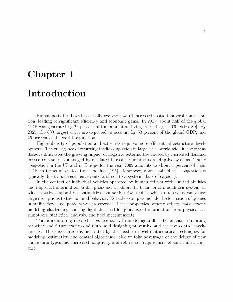
As illustrated by pilot projects such as the Mobile Millennium [19] and the Mobile Mil-lennium Stockholm [2], collection of anonymized individual sub-sampled trajectories could beconsidered a valid substitute to the installment and maintenance of fixed sensing infrastruc-ture in the future. In the Bay Area, the Mobile Millennium system receives several millionsdata points from GPS devices and GPS-enabled smart phones daily. A comparable volumeof data is received from loop detectors (see Figure 1.1). Fundamental differences betweenthese two data types are related to their spatial coverage, their noise statistics, and theirusability for traffic monitoring.
Figure 1.1: Traffic data collection in the Bay area.Left: loop detector locations at which count and occupancy are measured. Right: one day of GPSpoint speeds collected by the Mobile Millennium system.
Section 1.2. Hyperbolic conservation laws 3
Wide availability of traffic measurements collected along individual trajectories, i.e. in La-grangian coordinates, and from personal multi-purpose sensing devices with specific con-straints and error characteristics present new opportunities and challenges for traffic mod-eling and estimation, among which the design of models able to account for heterogeneousbehaviors, the design of transparent estimation methods and robust control algorithms ableto perform efficiently in the context of uncertain error propagation in complex systems.
Classical traffic models are based on flow and density information, and consists of mod-eling the average driver, or the average of drivers. This paradigm has provided reasonableresults, and significant insights on traffic behavior at a macroscopic level. GPS measurementsfrom individual drivers allow the observation of different driving behaviors and require thedesign of novel traffic models able to account for macroscopic phenomena resulting from theinteraction of heterogeneous agents.
The field of estimation is concerned with the construction of estimates that best rep-resent a process of interest. With the multiplication of the number of traffic sensors, thegrowing complexity of sensors and data processing algorithms, the need for estimation meth-ods able to properly account for error propagation increases. The choice of congestion controlalgorithms is also driven by the need to provide optimality guarantees in the presence of un-known error given the increasing volume of data used for the computation of the controlvariables.
This dissertation is centered on hyperbolic partial differential equations methods com-bined with filtering techniques from estimation theory and stabilization approaches for dy-namical systems. Relevant introductory material pertaining to these different fields is pre-sented in the following sections.
1.2 Hyperbolic conservation laws
1.2.1 A brief history of hyperbolic conservation laws
The conservation principle is one of the most fundamental modeling principles for phys-ical systems. Statements of conservation of mass, momentum, energy are at the center ofmodern classical physics. For distributed dynamical systems, this principle can be written inconservation law form with the use of partial differential equations (PDE). The problem ofwell-posedness of the partial differential equation is concerned with the existence, uniqueness,and continuous dependence of the solution to the problem data [89].
First existence results for scalar conservation laws in one dimension of space date backto [180]. For hyperbolic systems of conservation laws in one dimension of space, existenceresults were provided in [101] with the introduction of the random choice method. Existenceand uniqueness in the scalar case for several spatial dimensions were proven in [141], and tothis date constitute the only general results known on well-posedness for several dimensionsof space. Uniqueness for n × n hyperbolic systems of conservation laws in one-dimensionof space was shown only recently in [40]. Existence results can also be obtained using the
Section 1.2. Hyperbolic conservation laws 4
techniques developed in [40]. The global well-posedness of solutions to hyperbolic systemsof conservation laws in several dimensions of space is still a largely open problem.
Hyperbolic systems of conservation laws have been extensively applied to the modelingof physical systems. In the following section, we present seminal macroscopic traffic flowmodels based on hyperbolic systems of conservation laws.
1.2.2 Review of macroscopic traffic models
Macroscopic traffic modeling provides description of traffic phenomena as a continuumof vehicles, instead of modeling individual vehicle dynamics. Macroscopic traffic models arehistorically inspired from constitutive models for hydrodynamics systems, which share prop-erties with traffic flow.
First order scalar models of traffic.
Hydrodynamic models of traffic go back to the 1950’s with the work of Lighthill,Whitham and Richards [159, 189], who proposed the first model of the evolution of ve-hicle density on the highway using a first order scalar hyperbolic partial differential equation(PDE) referred to as the LWR PDE. Their model relies on the knowledge of an empiricallymeasured flux function, also called the fundamental diagram in transportation engineering,for which measurements go back to 1935 with the pioneering work of Greenshields [107].Numerous other flux functions have since been proposed in the hope of capturing effectsof congestion more accurately, in particular: Greenberg [106], Underwood [216], Newell-Daganzo [71, 177], and Papageorgiou [221]. The existence and uniqueness of an entropysolution to the Cauchy problem [198] for the class of scalar conservation laws to which theLWR PDE belongs go back to the work of Oleinik [180] and Kruzhkov [141], (see also theseminal article of Glimm [101]), which was extended later to the initial-boundary value prob-lem [15], and specifically instantiated for the scalar case with a concave flux function in [153],in particular for traffic in [205]. Numerical solutions of the LWR PDE go back to the semi-nal Godunov scheme [103, 156], which was shown to converge to the entropy solution of thefirst order hyperbolic PDE (in particular the LWR PDE). In the transportation engineeringcommunity, the Godunov scheme in the case of a triangular flux is known under the nameof Cell Transmission Model (CTM), which was brought to the field of transportation byDaganzo in 1995 [71, 72] (see [150] for the general case), and is one of the most used discretetraffic flow models in the literature today [48, 74, 126, 160, 174, 181, 220].
Set-valued fundamental diagrams.
The assumption of a Greenshields fundamental diagram or a triangular fundamentaldiagram, which significantly simplifies the analysis of the model algebraically, led to theaforementioned theoretical developments. Yet, experimental data clearly indicates that whilethe free flow part of a fundamental diagram can be approximated fairly accurately by a
Section 1.2. Hyperbolic conservation laws 5
straight line, the congested regime is set valued, and can hardly be characterized by asingle curve [219]. An approach to model the set-valuedness of the congested part of thefundamental diagram consists in using a second equation coupled with the mass conservationequation (i.e. the LWR PDE model). Such models go back to Payne [183] and Whitham [223]and generated significant research efforts, but led to models with inherent weaknesses pointedout by del Castillo [78] and Daganzo [73]. These weaknesses were ultimately addressed inseveral responses [13, 181, 230], leading to sustained research in this field.
The following sections are focused on the mathematical theory of scalar and non-scalartraffic flow models.
1.2.3 Scalar models of traffic flow
Classical scalar models of traffic consider the traffic state at a point x at time t to befully represented by the density ρ(t, x) of vehicles at this point. The evolution of the densityof vehicles can be modeled by a combination of physical principles, statistical properties,and empirical findings. All the models considered in this section are single-lane single-classmodels of traffic.
Continuous models
A classical state equation used to model the evolution of the density ρ(·, ·) of vehicles onthe road network is the LWR PDE [159, 189], which expresses the conservation of vehicleson road links:
∂tρ+ ∂xQ(ρ) = 0 (1.1)
where the flux function Q(·), assumed to be space-time invariant on limited space-timedomains, denotes the realized flux of vehicles with the density ρ, at the stationary state.The flux function, or fundamental diagram, is classically given by an empirical fit of therelation between density and flow. It can be equivalently given by an empirical fit V (·)of the relation between density and space-mean speed, which allows us to define the fluxfunction as:
Q(ρ) = q = ρ v = ρ V (ρ),
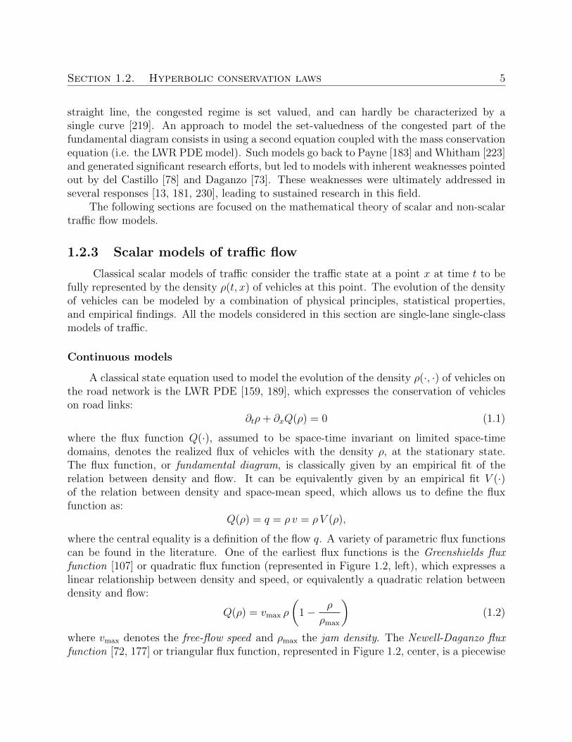
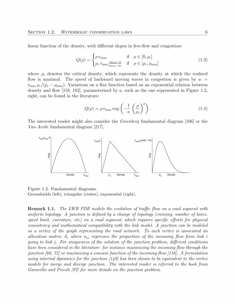
where the central equality is a definition of the flow q. A variety of parametric flux functionscan be found in the literature. One of the earliest flux functions is the Greenshields fluxfunction [107] or quadratic flux function (represented in Figure 1.2, left), which expresses alinear relationship between density and speed, or equivalently a quadratic relation betweendensity and flow:
Q(ρ) = vmax ρ
(1− ρ
ρmax
)(1.2)
where vmax denotes the free-flow speed and ρmax the jam density. The Newell-Daganzo fluxfunction [72, 177] or triangular flux function, represented in Figure 1.2, center, is a piecewise
Section 1.2. Hyperbolic conservation laws 6
linear function of the density, with different slopes in free-flow and congestion:
Q(ρ) =
ρ vmax if ρ ∈ [0, ρc]
ρc vmaxρmax−ρρmax−ρc if ρ ∈ [ρc, ρmax]
(1.3)
where ρc denotes the critical density, which represents the density at which the realizedflow is maximal. The speed of backward moving waves in congestion is given by w =vmax ρc/(ρc − ρmax). Variations on a flux function based on an exponential relation betweendensity and flow [158, 182], parameterized by a, such as the one represented in Figure 1.2,right, can be found in the literature:
Q(ρ) = ρ vmax exp
(−1
a
(ρ
ρc
)a). (1.4)
The interested reader might also consider the Greenberg fundamental diagram [106] or theVan-Aerde fundamental diagram [217].
Density
Flo
w
ρmax
vmax
ρmax
/4
Density
Flo
w
ρC
ρmax
vmax
ρc
Density
Flo
w
ρC
vmax
ρcexp(−1/a)
Figure 1.2: Fundamental diagrams.Greenshields (left), triangular (center), exponential (right).
Remark 1.1. The LWR PDE models the evolution of traffic flow on a road segment withuniform topology. A junction is defined by a change of topology (crossing, number of lanes,speed limit, curvature, etc) on a road segment, which requires specific efforts for physicalconsistency and mathematical compatibility with the link model. A junction can be modeledas a vertex of the graph representing the road network. To each vertex is associated anallocation matrix A, where aij expresses the proportion of the incoming flow from link igoing to link j. For uniqueness of the solution of the junction problem, different conditionshave been considered in the literature: for instance maximizing the incoming flow through thejunction [60, 72] or maximizing a concave function of the incoming flow [116]. A formulationusing internal dynamics for the junction [149] has been shown to be equivalent to the vertexmodels for merge and diverge junction. The interested reader is referred to the book fromGaravello and Piccoli [97] for more details on the junction problem.
Section 1.2. Hyperbolic conservation laws 7
For traffic applications, given an initial condition ρ0(·) defined on a stretch [0, L], usingthe LWR model requires solving the associated Cauchy problem, defined as the problem ofexistence and uniqueness of a solution to the LWR PDE with initial condition ρ0(·). If theinitial condition is piecewise constant (which is the case for many numerical approximations)and self-similar1, the Cauchy problem reduces to the Riemann problem (see Section 5.3.2).
For numerical computations, it is in general necessary to discretize the space of inde-pendent variables. The corresponding numerical schemes applied to the continuous modelsdescribed in this section can themselves be understood as discretized link models.
Discretized link models
Given a discretization grid defined by a space-step ∆x and a time-step ∆t, if we noteρni the discretized solution at i∆x, n∆t and Cni the cell defined by Cni = [n∆t, (n+ 1) ∆t]×[i∆x, (i+1) ∆x], the discretization of the LWR PDE using the Godunov scheme [103] reads:
ρn+1i = ρni +
∆t
∆x
(qG(ρni−1, ρ
ni )− qG(ρni , ρ
ni+1))
(1.5)
where the numerical Godunov flux qG(·, ·) is defined as follows for a concave flux functionQ(·) with a maximum at ρc:
qG(ρl, ρr) =
Q(ρl) if ρr ≤ ρl < ρc
Q(ρc) if ρr ≤ ρc ≤ ρl
Q(ρr) if ρc < ρr ≤ ρl
min(Q(ρl), Q(ρr)) if ρl < ρr
(1.6)
The Godunov scheme is a first order finite volume discretization scheme commonly used fornumerical computation of weak entropy solutions to one-dimensional conservations laws suchas the LWR PDE [156]. The design of the Godunov scheme dynamics (1.5) results from thefollowing steps:
1. At time n∆t, for each couple of neighboring cells Cni , Cni+1, compute the solution tothe Riemann problem defined at the intersection of cells Cni , Cni+1, by the left datum ρniand the right datum ρni+1.
2. At time (n + 1) ∆t, on each domain (n+ 1) ∆t × [i∆x, (i+ 1) ∆x] compute theaverage of the solution of the Riemann problem. Specifically, integrating the LWRPDE on the domain Cni , ∫∫
Cni
(∂ρ
∂t+∂Q(ρ)
∂x
)dxdt = 0 (1.7)
1A function f of n variables x1, . . . , xn is called self-similar if ∀α > 0 ∈ R, f(αx1, . . . , α xn) =f(x1, . . . , xn).
Section 1.2. Hyperbolic conservation laws 8
and applying the Stokes theorem on Cni to this equality yields:
∆x ρn+1i +
∫ (n+1) ∆t
n∆t
Q(ρ(t, i∆x))dt−∆x ρni −∫ (n+1) ∆t
n∆t
Q(ρ(t, (i+1) ∆x))dt = 0, (1.8)
where we note ρn+1i the space average of the solution to the Riemann problems on
(n+ 1) ∆t× [i∆x, (i+ 1) ∆x]. Since the solution to the Riemann problems are self-similar (see footnote 1), hence constant at i∆x and (i+ 1) ∆x, if we note respectivelyQ(ρni−1, ρ
ni ), Q(ρni , ρ
ni+1) the value of the corresponding flow at these locations over the
interval [n∆t, (n+ 1) ∆t], we obtain:
∆x ρn+1i −∆x ρni = ∆tQ(ρni−1, ρ
ni )−∆tQ(ρni , ρ
ni+1),
which is the dynamics equation (1.5) of the Godunov scheme.
The first step of the Godunov scheme is exact whereas the second step, through averaging,introduces numerical diffusion (see [156] for more details). The consequence of this diffusionon estimation is further discussed in Section 5.4.
Remark 1.2. It must be noted that grid-free algorithms allow the computation of numericalsolutions of scalar conservation laws without numerical diffusion [39], with a higher complex-ity in general. In the case of transportation, some algorithms have be shown to be exact forspecific fundamental diagrams and particular initial and boundary conditions [58, 59, 167,225].
The Godunov scheme has been shown to provide a numerical solution consistent withclassical traffic assumptions [150] and to be equivalent to the supply-demand formulation forconcave flux functions with a single maximum. In the case of a triangular flux function (1.3),the Godunov scheme reduces to the CTM [71, 72]:
qG(ρl, ρr) = min
(ρl V, ρc V, ρc V
ρmax − ρrρmax − ρc
).
Modeling capabilities of macroscopic traffic flow models can be extended by consideringnon-scalar models, presented in the following section.
1.2.4 Non-scalar models of traffic flow
Non-scalar models of traffic flow consider additional state variables and additional phys-ical principles to model traffic states. One of the first non-scalar traffic flow models is thePayne-Whitham model [183, 223]:
∂tρ+ ∂xq = 0
∂tv + v vx +c20ρ∂xρ = V (ρ)−v
τ.
(1.9)
Section 1.3. Estimation problem for distributed parameter systems 9
The first equation expresses the conservation of vehicles, and the second equation models theevolution of speed, which is subject to convection, anticipation, and relaxation (respectivelysecond and third left-hand side terms of second equation, and right-hand side term of thesecond equation).
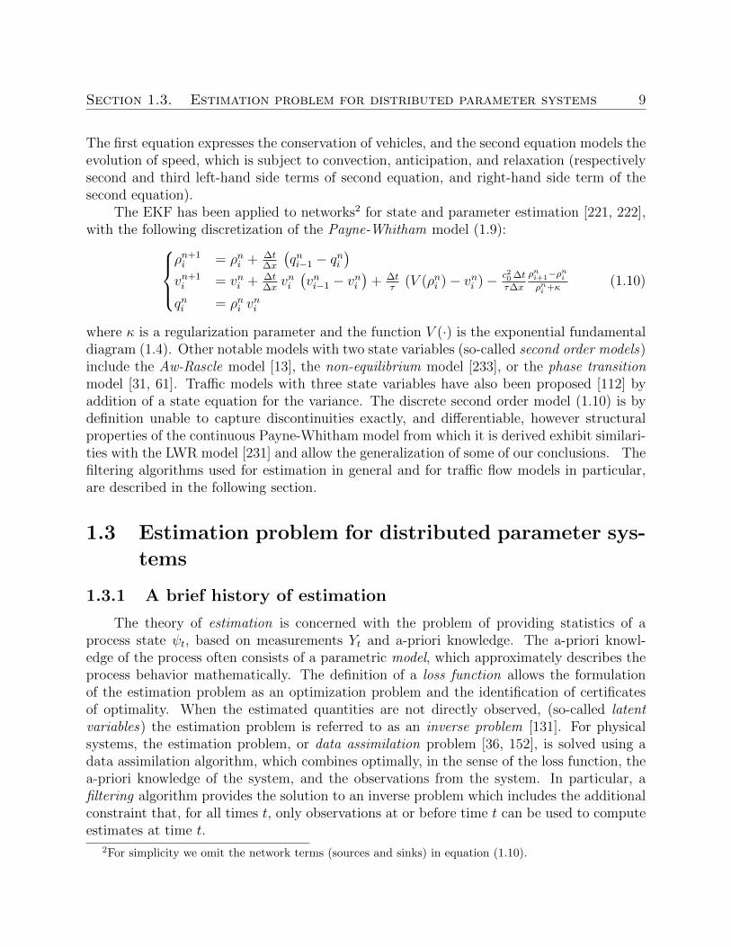
The EKF has been applied to networks2 for state and parameter estimation [221, 222],with the following discretization of the Payne-Whitham model (1.9):
ρn+1i = ρni + ∆t
∆x
(qni−1 − qni
)vn+1i = vni + ∆t
∆xvni(vni−1 − vni
)+ ∆t
τ(V (ρni )− vni )− c20 ∆t
τ∆x
ρni+1−ρniρni +κ
qni = ρni vni
(1.10)
where κ is a regularization parameter and the function V (·) is the exponential fundamentaldiagram (1.4). Other notable models with two state variables (so-called second order models)include the Aw-Rascle model [13], the non-equilibrium model [233], or the phase transitionmodel [31, 61]. Traffic models with three state variables have also been proposed [112] byaddition of a state equation for the variance. The discrete second order model (1.10) is bydefinition unable to capture discontinuities exactly, and differentiable, however structuralproperties of the continuous Payne-Whitham model from which it is derived exhibit similari-ties with the LWR model [231] and allow the generalization of some of our conclusions. Thefiltering algorithms used for estimation in general and for traffic flow models in particular,are described in the following section.
1.3 Estimation problem for distributed parameter sys-
tems
1.3.1 A brief history of estimation
The theory of estimation is concerned with the problem of providing statistics of aprocess state ψt, based on measurements Yt and a-priori knowledge. The a-priori knowl-edge of the process often consists of a parametric model, which approximately describes theprocess behavior mathematically. The definition of a loss function allows the formulationof the estimation problem as an optimization problem and the identification of certificatesof optimality. When the estimated quantities are not directly observed, (so-called latentvariables) the estimation problem is referred to as an inverse problem [131]. For physicalsystems, the estimation problem, or data assimilation problem [36, 152], is solved using adata assimilation algorithm, which combines optimally, in the sense of the loss function, thea-priori knowledge of the system, and the observations from the system. In particular, afiltering algorithm provides the solution to an inverse problem which includes the additionalconstraint that, for all times t, only observations at or before time t can be used to computeestimates at time t.
2For simplicity we omit the network terms (sources and sinks) in equation (1.10).
Section 1.3. Estimation problem for distributed parameter systems 10
The use of the quadratic loss function dates back to the estimation problem posed byGauss in the 18th century for astronomy [203, 204]. The solution proposed by Gauss is theso-called least-squares method, justified by the Gauss-Markov theorem [124]. The theoremproves that, assuming a linear observation model with additive white noise, the best linearunbiased estimator (BLUE) (best in the minimum variance sense), of a random process ψtcan be computed as the solution to the ordinary least squares (OLS) problem.
The role of the quadratic norm for estimation is further emphasized by a result fromSherman [199], which shows that for a large class of loss functions, which includes thequadratic loss function, the mean of the conditional distribution p(ψt|Yt) is optimal.
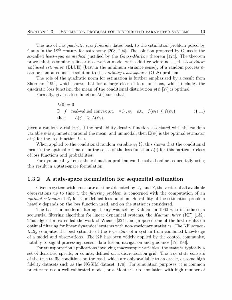
Formally, given a loss function L(·) such that:
L(0) = 0
∃ f real-valued convex s.t. ∀ψ1, ψ2 s.t. f(ψ1) ≥ f(ψ2) (1.11)
then L(ψ1) ≥ L(ψ2),
given a random variable ψ, if the probability density function associated with the randomvariable ψ is symmetric around the mean, and unimodal, then E(ψ) is the optimal estimatorof ψ for the loss function L(·).
When applied to the conditional random variable ψt|Yt, this shows that the conditionalmean is the optimal estimator in the sense of the loss function L(·) for this particular classof loss functions and probabilities.
For dynamical systems, the estimation problem can be solved online sequentially usingthis result in a state-space formulation.
1.3.2 A state-space formulation for sequential estimation
Given a system with true state at time t denoted by Ψt, and Yt the vector of all availableobservations up to time t, the filtering problem is concerned with the computation of anoptimal estimate of Ψt for a predefined loss function. Solvability of the estimation problemheavily depends on the loss function used, and on the statistics considered.
The basis for modern filtering theory was set by Kalman in 1960 who introduced asequential filtering algorithm for linear dynamical systems, the Kalman filter (KF) [132].This algorithm extended the work of Wiener [224] and proposed one of the first results onoptimal filtering for linear dynamical systems with non-stationary statistics. The KF sequen-tially computes the best estimate of the true state of a system from combined knowledgeof a model and observations. The KF has been widely applied by the control community,notably to signal processing, sensor data fusion, navigation and guidance [17, 193].
For transportation applications involving macroscopic variables, the state is typically aset of densities, speeds, or counts, defined on a discretization grid. The true state consistsof the true traffic conditions on the road, which are only available to an oracle, or some highfidelity datasets such as the NGSIM dataset [179]. For simulation purposes, it is commonpractice to use a well-calibrated model, or a Monte Carlo simulation with high number of
Section 1.3. Estimation problem for distributed parameter systems 11
samples, as a proxy for the true state (to avoid the so-called inverse crime [131], the modelused for estimation should be different from the model used for computing the true state).
Kalman filter
In his seminal article [132], Kalman provides a sequential algorithm to compute theBLUE of the state for dynamical systems, under additive white Gaussian noise, with adeterministic linear observation equation (this result was later extended to include additivewhite Gaussian observation noise). The Kalman filter is defined in a state-space model, whichconsists of a state equation and an observation equation.
We consider the following discrete linear model:
xt = At xt−1 + wt (1.12)
where we note At the state model or time-varying state transition matrix at time t, and wherethe random variable wt ∼ N (0,Wt) is a white noise vector which accounts for modelingerrors. In particular in this setting the true state Ψt is assumed to follow the dynamics Atwithout additional noise. Measurements are modeled by the linear observation equation:
yt = Ct Ψt + vt (1.13)
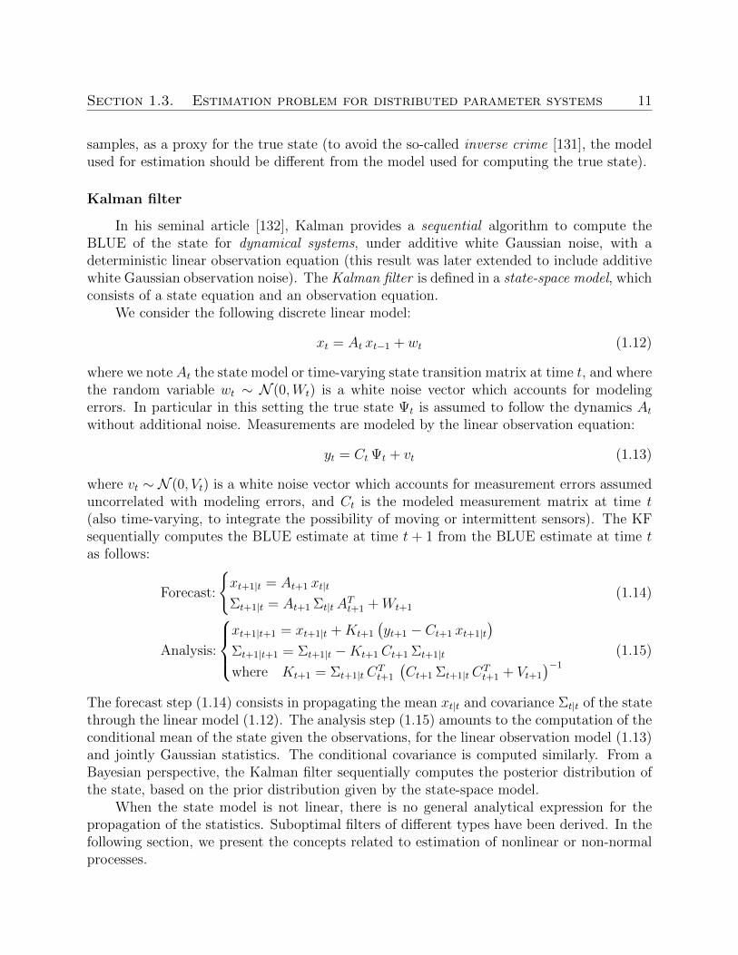
where vt ∼ N (0, Vt) is a white noise vector which accounts for measurement errors assumeduncorrelated with modeling errors, and Ct is the modeled measurement matrix at time t(also time-varying, to integrate the possibility of moving or intermittent sensors). The KFsequentially computes the BLUE estimate at time t + 1 from the BLUE estimate at time tas follows:
Forecast:
xt+1|t = At+1 xt|t
Σt+1|t = At+1 Σt|tATt+1 +Wt+1
(1.14)
Analysis:
xt+1|t+1 = xt+1|t +Kt+1
(yt+1 − Ct+1 xt+1|t
)Σt+1|t+1 = Σt+1|t −Kt+1Ct+1 Σt+1|t
where Kt+1 = Σt+1|tCTt+1
(Ct+1 Σt+1|tC
Tt+1 + Vt+1
)−1
(1.15)
The forecast step (1.14) consists in propagating the mean xt|t and covariance Σt|t of the statethrough the linear model (1.12). The analysis step (1.15) amounts to the computation of theconditional mean of the state given the observations, for the linear observation model (1.13)and jointly Gaussian statistics. The conditional covariance is computed similarly. From aBayesian perspective, the Kalman filter sequentially computes the posterior distribution ofthe state, based on the prior distribution given by the state-space model.
When the state model is not linear, there is no general analytical expression for thepropagation of the statistics. Suboptimal filters of different types have been derived. In thefollowing section, we present the concepts related to estimation of nonlinear or non-normalprocesses.
Section 1.4. Contributions and organization of the dissertation 12
1.3.3 Normality and nonlinearity
The statistical assumptions on the processes ψt and Yt are tied to prior knowledge of thegenerative distributions. However, a significant computational argument in favor of the useof normal statistics is the optimality guarantee provided by combining the two argumentsabove. Without any assumption on the statistics, the Gauss-Markov theorem states that theBLUE is given by the solution to the OLS algorithm. Sherman’s result for the class of lossfunctions (1.11) states that the solution of the OLS is the conditional mean. In the Gaussiancase the conditional mean is linear, hence it is also the solution of the OLS with constraintthat the estimator be linear. Hence the BLUE of the process is optimal, without restrictionof linearity on the estimator, if we assume that the statistics are Gaussian.
The need for solving the inverse problem for increasingly complex systems, for which theclassical assumptions of linearity of the dynamics and normality of the error terms break,has motivated the development of suboptimal sequential estimation algorithms. Subopti-mal sequential estimation algorithms can be derived from the Kalman filter using differentmethods:
1. Deterministic filters: extended Kalman filter (EKF) [9], unscented Kalman filter (UKF)[129].
2. Stochastic filters: ensemble Kalman filter (EnKF) [93], particle filter (PF) [163].
Stochastic methods consider propagating the state through the nonlinear model using a sam-ple representation. Deterministic methods consist in propagating analytical approximationsof low order moments through the model. Stochastic methods in general require samplingschemes and pseudo-random generators for the correct execution of the filters, unlike deter-ministic methods.
For traffic applications, it is also important to mention the mixture Kalman filter(MKF) [51], which provides optimality guarantees for conditionally linear systems. In thisdissertation, we analyze the error structure resulting from the propagation of uncertaintyin the initial condition of a Cauchy problem and assess the performances of the EKF andEnKF for realistic scalar traffic models.
1.4 Contributions and organization of the dissertation
1.4.1 Contributions
The contributions of this dissertation encompass the theory of hyperbolic conservationlaws for traffic estimation and control. They include contributions to mathematical modeling,theory of partial differential equations, numerical analysis, control theory, filtering, and dataanalysis.
Section 1.4. Contributions and organization of the dissertation 13
Phase transition traffic flow model [31, 32].
• Definition of a phase transition traffic flow model as a perturbation of the classicalLighthill-Whitham-Richards scalar traffic flow model.
• Well-posedness constraints on the classical fundamental diagram for instantiations onthe well-known Newell-Daganzo, Greenshield, Li fundamental diagrams.
• Construction of a Riemann solver in the case of a Newell-Daganzo, Greenshield, Lifundamental diagram.
Analysis of complex traffic phenomena [30, 23].
• Investigation of the existence of complex macroscopic traffic phenomena in high reso-lution data.
• Implementation of a modified Godunov scheme able to account for non-convexity ofmodel state space in the phase transition model.
• Comparison of time-space diagram reconstruction performance for phase transitionmodel and scalar traffic models.
Error propagation in filtering algorithms [25].
• Construction of the solution to a Riemann problem with random initial datum.
• Analysis of uncertainty structure arising in the solution to the Riemann problem withrandom initial datum.
• Quantification of error propagation resulting from non differentiability of Godunovdiscrete time dynamics at the location of stationary shock waves.
Boundary stabilization of entropic solutions to scalar conservation laws [27, 28].
• Approximation of a solution to a scalar conservation law by a piecewise differentiablesolution in the case of a traffic model.
• Differentiation of Lyapunov function candidate for an entropic solution to the initialboundary value problem associated with a scalar conservation law.
• Design of weak boundary conditions that maximize the decrease of the Lyapunovfunction candidate.
Section 1.4. Contributions and organization of the dissertation 14
1.4.2 Additional contributions
Along with the main contributions outlined in the previous subsection, several inde-pendent and related research endeavors led to significant results, presented in associateddissertation works.
Velocity formulation for scalar hyperbolic conservation laws [227].
• Derivation of a velocity PDE (v-PDE) for scalar conservation laws.
• Proof of equivalence of the weak entropy solution to the v-PDE with the weak entropysolution to the corresponding LWR PDE for the Greenshields flux function.
• Design of a numerical scheme derived from the Godunov scheme, for the velocityformulation.
• Real-time data assimilation with the v-PDE and traffic data on the Bay Area trans-portation network.
Stochastic routing algorithm for on-time arrival problem [191, 35].
• Design of a routing algorithm based on the Fast Fourier Transform for fast computationof the solution to the on-time arrival problem.
• Definition of an optimal order for computing the policy and experimental results ofthe order of magnitude computation time gain.
• Extensions to time-varying and correlated link travel-time distributions case.
• iPhone app design and deployment of the routing algorithm on the Bay Area trans-portation network.
Additional contributions include:
• Numerical analysis results for the LWR equation [24].
• Data analysis of radar measurements and identification of experimental relation be-tween speed variance and traffic flow [29].
• Forecast algorithms for distributed systems based on kernel methods in a convex opti-mization framework [26] and using Bayesian networks [192].
• Deployment of the Mobile Millennium Stockholm [2].
Section 1.4. Contributions and organization of the dissertation 15
1.4.3 Organization of the dissertation
The dissertation is organized as follows.Chapter 2 presents a novel 2× 2 phase transition model introduced in this dissertation.
The original phase transition model is presented, as well as its limitations for traffic modeling.A new perspective on the derivation of the phase transition model as a perturbation ofclassical macroscopic traffic model resulting from heterogeneous driving behavior is proposed,and constraints required for the well-posedness of the system of partial differential equationsare derived. The model is instantiated on several well-known traffic models, and a Riemannsolver is constructed in each case.
Chapter 3 presents an analysis of the performance of the phase transition model for theconstruction of spatio-temporal traffic patterns using high-resolution field data. Physicalinterpretations of the nature of the waves introduced by the model are proposed, discussed,and critically assessed in the light of experimental observations. An itemized implementationof a modified Godunov scheme is proposed.
Chapter 4 consists of a review of novel estimation methods proposed in this work fordistributed parameter systems. The framework of Bayesian networks, which allows thecomputationally efficient modeling of non-independence structure of joint random variables,is presented and the specific assumptions made for traffic models are described, as well asnumerical results for a Bay Area stretch of road. Finally, a novel technique for convexidentification of optimal state space representation using kernel methods is described.
Chapter 5 presents an analytical and numerical study of the structure of the true un-certainty associated with the propagation of uncertainty on the initial condition of an initialboundary value problem associated with a scalar hyperbolic conservation law. A solution tothe Riemann problem with stochastic datum is proposed in the case of a shock wave, and themixture nature of the resulting random field is shown. The consequence of the non-linearityof the flow of the PDE is assessed numerically on several benchmark estimation tests usingthe EKF and the EnKF on scenarios relevant for traffic. The non-differentiability of theGodunov scheme at the location of stationary shock waves is shown, and the consequenceon the accuracy of the estimates produced by the EKF is assessed on a test case.
Chapter 6 proposes the approximation of BV solutions to scalar conservation laws bypiecewise differentiable solutions, and presents a differentiation of an associated Lyapunovfunction candidate. A greedy controller is derived semi-analytically at each boundary. Thecontroller accounts for weak boundary conditions while maximizing the decrease rate of theLyapunov function candidate.
Section 7 summarizes the contributions of this dissertation work, and describes novelresearch tracks opened by the results obtained.
16
Chapter 2
A general phase transition model forvehicular traffic
In this chapter, we present a novel 2 × 2 hyperbolic system of conservation laws formacroscopic traffic modeling. The use of non-scalar macroscopic models of traffic flow hasbeen motivated by experimental data suggesting the existence of complex traffic phenomenathat could not be modeled using a scalar represention. The model introduced in this chapteris shown to not exhibit most of the issues existing in most of the so-called higher-ordermodels of traffic flow available today, such as vanishing velocities below jam density, whichis not a classical assumption in traffic theory [98].
The phase transition model introduced in this chapter extends the work of Colombo [62].In agreement with the remarks from Kerner [134, 135] affirming that traffic flow presents threedifferent behaviors, free-flow, wide moving jams, and synchronized flow, Colombo proposed a2×2 phase transition model [61, 62] which considers congestion and free-flow in traffic as twodifferent phases, governed by distinct evolutionary laws (see also [102] for a phase transitionversion of the Aw-Rascle model). The well-posedness of this model was proved in [63] usingwavefront tracking techniques [39, 117]. In the phase transition model, the evolution of theparameters is governed by two distinct dynamics; in free-flow, the Colombo phase transitionmodel is a classical first order model (LWR PDE), whereas in congestion a similar equationgoverns the evolution of an additional state variable, the linearized momentum q. Themotivation for an extension of the 2 × 2 phase transition model comes from the followingitems, which are addressed by the class of models presented in this chapter:
i Phases gap. The phase transition model introduced by Colombo in [61] uses a Green-shields flux function to describe free-flow, which despite its simple analytical expressionyields a fundamental diagram which is not connected and thus a complex definition of thesolution to the Riemann problem between two different phases. We solve this problem byintroducing a Newell-Daganzo flux function for free-flow, which creates a non-empty in-tersection between the congested phase and the free-flow phase, called metastable phase.It alleviates the inconvenience of having to use a shock-like phase transition in many
Section 2.1. The Colombo phase transition model 17
cases of the Riemann problem between two different phases.
ii Definition of a general class of set-valued fundamental diagrams. The work presentedin [62] enables the definition of a set-valued fundamental diagram for the expression ofthe velocity function introduced. However, experimental data shows that several types offundamental diagrams exist, with different congested domain shapes. Here, we providea method to build an arbitrary set-valued fundamental diagram which in a special casecorresponds to the fundamental diagram introduced in [61]. This enables us to define acustom-made set-valued fundamental diagram.
This chapter is organized as follows. Section 2.1 presents the fundamental features ofthe Colombo phase transition model [62], which serves as the basis for the present work.In Section 2.2, we introduce the modifications to the Colombo phase transition model, andintroduce the notion of standard state which provides the basis for the construction of aclass of 2 × 2 traffic models. We also assess general conditions which enable us to extendthe results obtained for the original Colombo phase transition model to these new models.Finally, this section presents a modified Godunov scheme which can be used to solve theequations numerically. The two following sections instantiate the constructed class of modelsfor two specific flux functions, which are the Newell-Daganzo (affine) flux function (Section2.3) and the Greenshields (parabolic concave) flux function (Section 2.4). Each of thesesections includes a discussion of the choice of parameters needed for each of the models, thesolution to the Riemann problem, a description of the specific properties of the model, anda validation of the numerical results using a benchmark test.
2.1 The Colombo phase transition model
The original Colombo phase transition model [61, 62] is a set of two coupled PDEsrespectively valid in a free-flow regime and congested regime:
∂tρ+ ∂x(ρ vf (ρ)) = 0 in free-flow (Ωf )∂tρ+ ∂x(ρ vc(ρ, q)) = 0
∂tq + ∂x((q − q∗) vc(ρ, q)) = 0in congestion (Ωc)
(2.1)
where the state variables ρ and q denote respectively the density and the linearized momen-tum [62]. Ωf and Ωc are the respective domains of validity of the free-flow and congestedequations of the model and are explicited below. The term q∗ is a characteristic parameterof the road under consideration. An empirical relation expresses the velocity v as a functionof density in free-flow: v := vf (ρ), and as a function of density and linearized momentum incongestion: v := vc(ρ, q). Following usual choices for traffic applications [97], the functionsbelow are used:
vf (ρ) =(
1− ρ
R
)V and vc(ρ, q) =
(1− ρ
R
) q
ρ
Section 2.1. The Colombo phase transition model 18
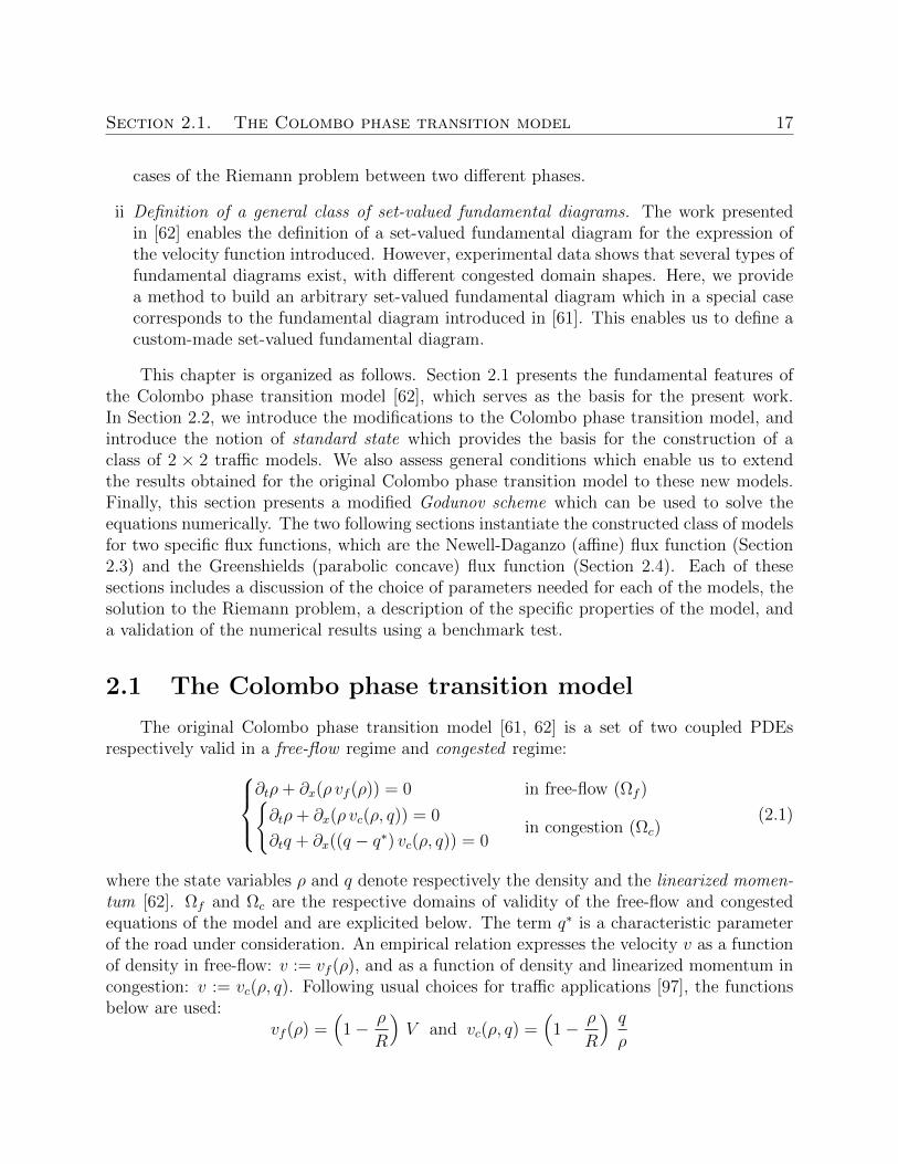
where R is the maximal density or jam density and V is the maximal free-flow speed. Therelation for free-flow is the Greenshields model [107] mentioned earlier while the secondrelation has been introduced in [61]. Since Ωc has to be an invariant domain [198] for thecongested dynamics from system (2.1), and according to the definition of v, the free-flow andcongested domains are defined as follows:
Ωf = (ρ, q) ∈ [0, R]× [0,+∞[ , vf (ρ) ≥ Vf− , q = ρ V Ωc =
(ρ, q) ∈ [0, R]× [0,+∞[ , vc(ρ, q) ≤ Vc+ , Q−−q∗
R≤ q−q∗
ρ≤ Q+−q∗
R
where Vf− is the minimal velocity in free-flow and Vc+ is the maximal velocity in congestionsuch that Vc+ < Vf− < V . R is the maximal density and Q− and Q+ are respectively theminimal and maximal values for q. The fundamental diagram in (ρ, q) coordinates and in(ρ, ρ v) coordinates is presented in Figure 2.1.
Figure 2.1: Colombo phase transition model.Left: Fundamental diagram in state space coordinates (ρ, q). Right: Fundamental diagram indensity flux coordinates (ρ, ρ v).
Remark 2.1. The congested part of system (2.1) is strictly hyperbolic if and only if the twoeigenvalues of its Jacobian are real and distinct for all states (ρ, q) ∈ Ωc.
Remark 2.2. The 1-Lax curves are straight lines going through (0, q∗) in (ρ, q) coordinateswhich means that along these curves shocks and rarefactions exist and coincide [210]. Onemust note that the 1-Lax field is not genuinely non-linear (GNL). Indeed the 1-Lax curves arelinearly degenerate (LD) for q = q∗ and GNL otherwise with rarefaction waves propagatingin different directions relatively to the eigenvectors depending on the sign of q − q∗. The2-Lax curves, which are straight lines going through the origin in (ρ, ρ v) coordinates, arealways LD.
Section 2.2. Extension of the Colombo phase transition model 19
2.2 Extension of the Colombo phase transition model
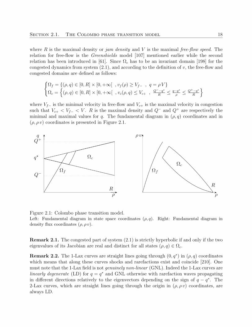
The approach developed by Colombo provides a fundamental diagram which is thickin congestion (Figure 2.1), and thus can model clouds of points observed experimentally(Figure 2.2). We propose to extend this approach by considering the second equation in
Figure 2.2: Fundamental diagram in density flux coordinates from a street in Rome.In congestion (high densities) the flux is multi-valued. Count C and velocity v were recorded everyminute during one week. Flux Q was computed from the count. Density ρ was computed from fluxand velocity according to the expression Q = ρ v (see [24] for an extensive analysis of this dataset).
congestion as modeling a perturbation [230, 233]. The standard state (Definition 2.1) wouldbe the usual one-dimensional fundamental diagram, with dynamics described by the conser-vation of mass. Perturbations can move the system off standard state, leading the diagramto span a two-dimensional area in congestion. A single-valued map is able to describe thefree-flow mode, which is therefore completely described by the free-flow standard state.
Definition 2.1. We call standard state the set of states described by a one dimensionalfundamental diagram and the classical LWR PDE. In the following we respectively refer tothe standard velocity and standard flux as the velocity and flux at the standard state.
In this section we present analytical requirements on the velocity function in congestionwhich, given the work done in [62], enable us to construct a 2 × 2 phase transition model.These models provide support for a physically correct, mathematically well-posed initial-boundary value problem which can model traffic phenomena where the density and the floware independent quantities in congestion, allowing for multiple values of the flow for a givenvalue of the density. Our framework allows the definition of the two dimensional zone spanby the congestion phase according to the reality of the local traffic nature, which is notalways possible with the original Colombo phase transition model.
Section 2.2. Extension of the Colombo phase transition model 20
2.2.1 Analysis of the standard state
We consider the density variable ρ to belong to the interval [0, R] where R is the maximaldensity. Given the critical density1 σ in (0, R], we define the standard velocity vs(·) on [0, R]by:
vs(ρ) :=
V for ρ ∈ [0, σ]
vsc(ρ) for ρ ∈ [σ,R]
where V is the free-flow speed and vsc(·) is in C∞((σ,R),R+). It is important to note thatvsc(·) is a function of ρ only, as it is the case for the classical fundamental diagram. Thestandard flux Qs(·) is thus defined on [0, R] by:
Qs(ρ) := ρ vs(ρ) =
Qf (ρ) := ρ V for ρ ∈ [0, σ]
Qsc(ρ) := ρ vsc(ρ) for ρ ∈ [σ,R].
In agreement with traffic flow features, the congested standard flux Qsc(ρ) must satisfy the
following requirements (which are consistent with the ones given in [77]).
i Flux vanishes at the maximal density : Qsc(R) = 0.
This condition encodes the physical situation in which the jam density has been reached.The corresponding velocity and flux of vehicles on the highway is zero.
ii Flux is a decreasing function of density in congestion: dQsc(ρ)/dρ ≤ 0.
This is required as a defining property of congestion. It implies that dvsc(ρ)/dρ ≤ 0.
iii Continuity of the flux at the critical density : Qsc(σ) = Qf (σ).
Even if some models account for a discontinuous flux at capacity, the capacity dropphenomenon [135], we assume, following most of the transportation community, that theflux at the standard state is a continuous function of density.
iv Concavity of the flux in congestion: Qsc(·).
The flux function at the standard state Qsc(·) must be concave on [σ, σi] and convex on
[σi, R] where σi is in (σ,R]. Given the experimental datasets obtained for congestion(Figure 2.2), it is not clear in practice if the standard flux is concave or convex incongestion. The assumption made here is motivated in Remark 2.8.
Remark 2.3. In this chapter we instantiate the general model proposed on the most commonstandard flux functions, i.e. linear or concave, but the framework developed here applies toflux functions with changing concavity such as the Li flux function [158], although it yieldsa significantly more complex analysis.
1Density for which the flux is maximal at the standard state. At this density the system switches betweenfree-flow and congestion.
Section 2.2. Extension of the Colombo phase transition model 21
2.2.2 Analysis of the perturbation
Model outline
In this section we introduce a perturbation q to the standard velocity in congestion.
Definition 2.2. The perturbed velocity function vc(·, ·) is defined on Ωc by:
vc(ρ, q) = vsc(ρ) (1 + q) (2.2)
where vsc(·) ∈ C∞((σ−, R),R+) is the congested standard velocity function.
The standard state corresponds to q = 0, and the evolution of (ρ, q) is described similarlyto the classical Colombo phase transition model [62] by:
∂tρ+ ∂x(ρ v) = 0 in free-flow∂tρ+ ∂x(ρ v) = 0
∂tq + ∂x(q v) = 0in congestion
(2.3)
with the following expression of the velocity:
v =
vf (ρ) := V in free-flow
vc(ρ, q) in congestion.(2.4)
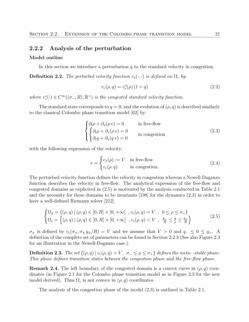
The perturbed velocity function defines the velocity in congestion whereas a Newell-Daganzofunction describes the velocity in free-flow. The analytical expression of the free-flow andcongested domains as explicited in (2.5) is motivated by the analysis conducted in Table 2.1and the necessity for these domains to be invariants [198] for the dynamics (2.3) in order tohave a well-defined Riemann solver [212].
Ωf = (ρ, q) | (ρ, q) ∈ [0, R]× [0,+∞[ , vc(ρ, q) = V , 0 ≤ ρ ≤ σ+Ωc =
(ρ, q) | (ρ, q) ∈ [0, R]× [0,+∞[ , vc(ρ, q) < V , q−
R≤ q
ρ≤ q+
R
(2.5)
σ± is defined by vc(σ±, σ± q±/R) = V and we assume that V > 0 and q− ≤ 0 ≤ q+. Adefinition of the complete set of parameters can be found in Section 2.2.3 (See also Figure 2.3for an illustration in the Newell-Daganzo case.).
Definition 2.3. The set (ρ, q) | vc(ρ, q) = V , σ− ≤ ρ ≤ σ+ defines the meta- -stable phase.This phase defines transition states between the congestion phase and the free-flow phase.
Remark 2.4. The left boundary of the congested domain is a convex curve in (ρ, q) coor-dinates (in Figure 2.1 for the Colombo phase transition model as in Figure 2.3 for the newmodel derived). Thus Ωc is not convex in (ρ, q) coordinates.
The analysis of the congestion phase of the model (2.3) is outlined in Table 2.1.
Section 2.2. Extension of the Colombo phase transition model 22
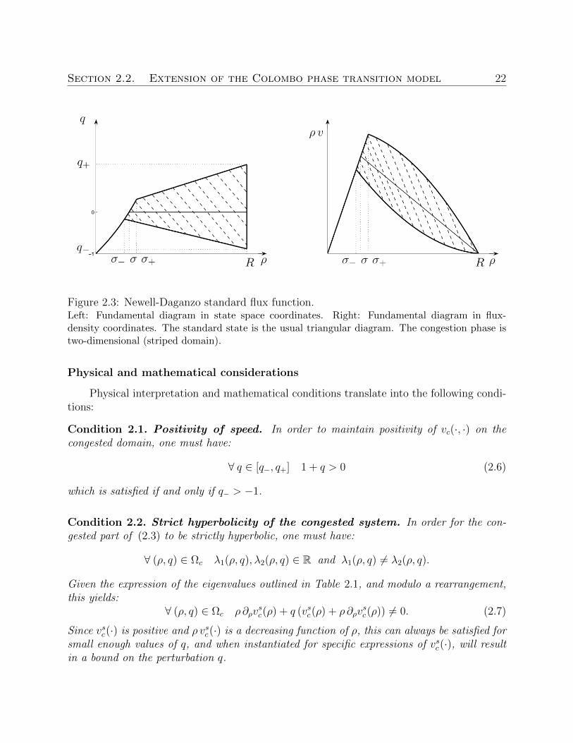
Figure 2.3: Newell-Daganzo standard flux function.Left: Fundamental diagram in state space coordinates. Right: Fundamental diagram in flux-density coordinates. The standard state is the usual triangular diagram. The congestion phase istwo-dimensional (striped domain).
Physical and mathematical considerations
Physical interpretation and mathematical conditions translate into the following condi-tions:
Condition 2.1. Positivity of speed. In order to maintain positivity of vc(·, ·) on thecongested domain, one must have:
∀ q ∈ [q−, q+] 1 + q > 0 (2.6)
which is satisfied if and only if q− > −1.
Condition 2.2. Strict hyperbolicity of the congested system. In order for the con-gested part of (2.3) to be strictly hyperbolic, one must have:
∀ (ρ, q) ∈ Ωc λ1(ρ, q), λ2(ρ, q) ∈ R and λ1(ρ, q) 6= λ2(ρ, q).
Given the expression of the eigenvalues outlined in Table 2.1, and modulo a rearrangement,this yields:
∀ (ρ, q) ∈ Ωc ρ ∂ρvsc(ρ) + q (vsc(ρ) + ρ ∂ρv
sc(ρ)) 6= 0. (2.7)
Since vsc(·) is positive and ρ vsc(·) is a decreasing function of ρ, this can always be satisfied forsmall enough values of q, and when instantiated for specific expressions of vsc(·), will resultin a bound on the perturbation q.
Section 2.2. Extension of the Colombo phase transition model 23
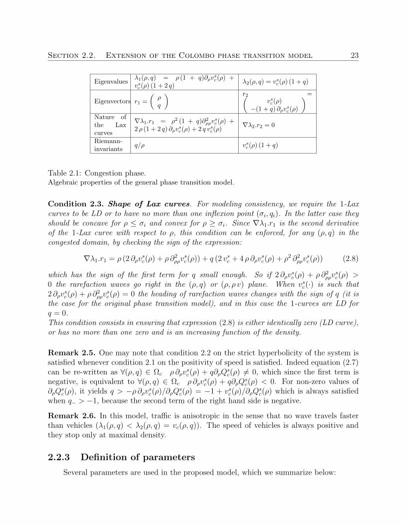
Eigenvaluesλ1(ρ, q) = ρ (1 + q)∂ρv
sc(ρ) +
vsc(ρ) (1 + 2 q)λ2(ρ, q) = vsc(ρ) (1 + q)
Eigenvectors r1 =
(ρq
) r2 =(vsc(ρ)
−(1 + q) ∂ρvsc(ρ)
)Nature ofthe Laxcurves
∇λ1.r1 = ρ2 (1 + q)∂2ρρvsc(ρ) +
2 ρ (1 + 2 q) ∂ρvsc(ρ) + 2 q vsc(ρ)
∇λ2.r2 = 0
Riemann-invariants
q/ρ vsc(ρ) (1 + q)
Table 2.1: Congestion phase.Algebraic properties of the general phase transition model.
Condition 2.3. Shape of Lax curves. For modeling consistency, we require the 1-Laxcurves to be LD or to have no more than one inflexion point (σi, qi). In the latter case theyshould be concave for ρ ≤ σi and convex for ρ ≥ σi. Since ∇λ1.r1 is the second derivativeof the 1-Lax curve with respect to ρ, this condition can be enforced, for any (ρ, q) in thecongested domain, by checking the sign of the expression:
∇λ1.r1 = ρ (2 ∂ρvsc(ρ) + ρ ∂2
ρρvsc(ρ)) + q (2 vsc + 4 ρ ∂ρv
sc(ρ) + ρ2 ∂2
ρρvsc(ρ)) (2.8)
which has the sign of the first term for q small enough. So if 2 ∂ρvsc(ρ) + ρ ∂2
ρρvsc(ρ) >
0 the rarefaction waves go right in the (ρ, q) or (ρ, ρ v) plane. When vsc(·) is such that2 ∂ρv
sc(ρ) + ρ ∂2
ρρvsc(ρ) = 0 the heading of rarefaction waves changes with the sign of q (it is
the case for the original phase transition model), and in this case the 1-curves are LD forq = 0.This condition consists in ensuring that expression (2.8) is either identically zero (LD curve),or has no more than one zero and is an increasing function of the density.
Remark 2.5. One may note that condition 2.2 on the strict hyperbolicity of the system issatisfied whenever condition 2.1 on the positivity of speed is satisfied. Indeed equation (2.7)can be re-written as ∀(ρ, q) ∈ Ωc ρ ∂ρv
sc(ρ) + q∂ρQ
sc(ρ) 6= 0, which since the first term is
negative, is equivalent to ∀(ρ, q) ∈ Ωc ρ ∂ρvsc(ρ) + q∂ρQ
sc(ρ) < 0. For non-zero values of
∂ρQsc(ρ), it yields q > −ρ ∂ρvsc(ρ)/∂ρQ
sc(ρ) = −1 + vsc(ρ)/∂ρQ
sc(ρ) which is always satisfied
when q− > −1, because the second term of the right hand side is negative.
Remark 2.6. In this model, traffic is anisotropic in the sense that no wave travels fasterthan vehicles (λ1(ρ, q) < λ2(ρ, q) = vc(ρ, q)). The speed of vehicles is always positive andthey stop only at maximal density.
2.2.3 Definition of parameters
Several parameters are used in the proposed model, which we summarize below:
Section 2.2. Extension of the Colombo phase transition model 24
i The free-flow speed V .
ii The maximal density R.
iii The critical density σ at standard state.
iv The critical density for the lower bound of the diagram σ−.
v The critical density for the upper bound of the diagram σ+.
These parameters can be identified from experimental data, and enable the definition of theparameters q− and q+. Figure 2.3 graphically summarizes the definition of the parameterschosen. One must note that the constraints on q−, q+ detailed in (2.6)-(2.7)-(2.8) translateinto constraints on σ−, σ+, which cannot be freely chosen.
2.2.4 Cauchy problem
In this section we define a solution to the Cauchy problem for the system (2.3). Follow-ing [62], we use a definition derived from [39].
Definition 2.4. Given T in R+, u0 in L1(R; Ωf ∪ Ωc) ∩ BV (R; Ωf ∪ Ωc), an admissiblesolution to the corresponding Cauchy problem for (2.3) is a function u(·, ·) in L1([0, T ] ×R; Ωf ∪ Ωc) ∩BV ([0, T ]× R; Ωf ∪ Ωc) such that the following holds.
i For all t in [0, T ], t 7→ u(t, .) is Lipshitz continuous with respect to the L1 norm.
ii For all functions ϕ in C1c ([0, T ]× R 7→ R) with compact support contained in u−1(Ωf ):∫ T
0
∫R
(u(t, x) ∂tϕ(t, x) +Qf (u(t, x))∂xϕ(t, x)) dxdt+
∫Ru0(x)ϕ(0, x)dx = 0.
iii For all functions ϕ in C1c ([0, T ]× R 7→ R2) with compact support contained in u−1(Ωc):∫ T
0
∫R
(u(t, x) ∂tϕ(t, x) +Qc(u(t, x))∂xϕ(t, x)) dxdt+
∫Ru0(x)ϕ(0, x)dx = 0.
iv The set of points (t, x) for which there is a change of phase is the union of a finitenumber of Lipschitz curves pi : [0, T ) 7→ R such that if ∃i 6= j and ∃τ ∈ [0, T ] such thatpi(τ) = pj(τ) then ∀t ∈ [τ, T ] we have pi(t) = pj(t).
v For all points (t, x) where there is a change of phase, let Λ = pi(t+), and introducing the
left and right flow at (t, x):
F l =
ρ(t, x−)V if ρ(t, x−) ∈ Ωf
ρ(t, x−) vc(ρ(t, x−), q(t, x−)) if ρ(t, x−) ∈ Ωc
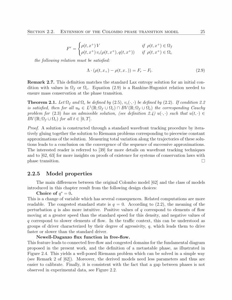
Section 2.2. Extension of the Colombo phase transition model 25
F r =
ρ(t, x+)V if ρ(t, x+) ∈ Ωf
ρ(t, x+) vc(ρ(t, x+), q(t, x+)) if ρ(t, x+) ∈ Ωc
the following relation must be satisfied:
Λ · (ρ(t, x+)− ρ(t, x−)) = Fr − Fl. (2.9)
Remark 2.7. This definition matches the standard Lax entropy solution for an initial con-dition with values in Ωf or Ωc. Equation (2.9) is a Rankine-Hugoniot relation needed toensure mass conservation at the phase transition.
Theorem 2.1. Let Ωf and Ωc be defined by (2.5), vc(·, ·) be defined by (2.2). If condition 2.2is satisfied, then for all u0 ∈ L1(R; Ωf ∪ Ωc) ∩ BV (R; Ωf ∪ Ωc) the corresponding Cauchyproblem for (2.3) has an admissible solution, (see definition 2.4) u(·, ·) such that u(t, ·) ∈BV (R; Ωf ∪ Ωc) for all t ∈ [0, T ].
Proof. A solution is constructed through a standard wavefront tracking procedure by itera-tively gluing together the solution to Riemann problems corresponding to piecewise constantapproximations of the solution. Measuring total variation along the trajectories of these solu-tions leads to a conclusion on the convergence of the sequence of successive approximations.The interested reader is referred to [39] for more details on wavefront tracking techniquesand to [62, 63] for more insights on proofs of existence for systems of conservation laws withphase transition.
2.2.5 Model properties
The main differences between the original Colombo model [62] and the class of modelsintroduced in this chapter result from the following design choices:
Choice of q∗ = 0.This is a change of variable which has several consequences. Related computations are morereadable. The congested standard state is q = 0. According to (2.2), the meaning of theperturbation q is also more intuitive. Positive values of q correspond to elements of flowmoving at a greater speed than the standard speed for this density, and negative values ofq correspond to slower elements of flow. In the traffic context, this can be understood asgroups of driver characterized by their degree of agressivity, q, which leads them to drivefaster or slower than the standard driver.
Newell-Daganzo flux function in free-flow.This feature leads to connected free-flow and congested domains for the fundamental diagramproposed in the present work, and the definition of a metastable phase, as illustrated inFigure 2.4. This yields a well-posed Riemann problem which can be solved in a simple way(see Remark 2 of [62]). Moreover, the derived models need less parameters and thus areeasier to calibrate. Finally, it is consistent with the fact that a gap between phases is notobserved in experimental data, see Figure 2.2.
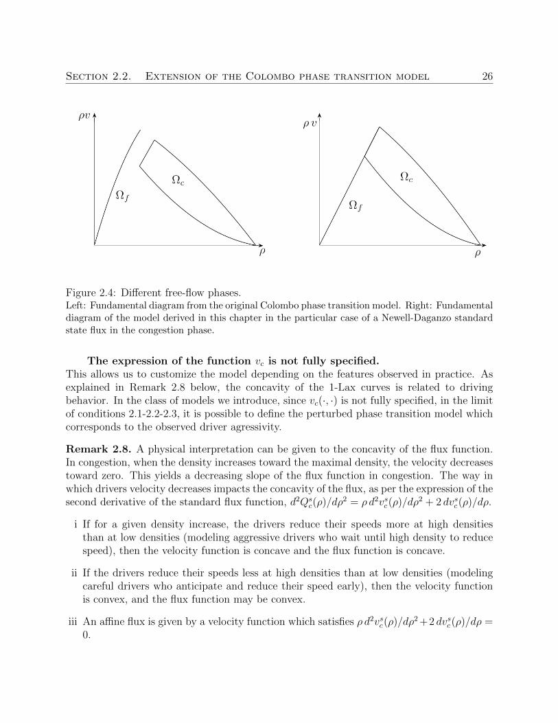
Section 2.2. Extension of the Colombo phase transition model 26
Figure 2.4: Different free-flow phases.Left: Fundamental diagram from the original Colombo phase transition model. Right: Fundamentaldiagram of the model derived in this chapter in the particular case of a Newell-Daganzo standardstate flux in the congestion phase.
The expression of the function vc is not fully specified.This allows us to customize the model depending on the features observed in practice. Asexplained in Remark 2.8 below, the concavity of the 1-Lax curves is related to drivingbehavior. In the class of models we introduce, since vc(·, ·) is not fully specified, in the limitof conditions 2.1-2.2-2.3, it is possible to define the perturbed phase transition model whichcorresponds to the observed driver agressivity.
Remark 2.8. A physical interpretation can be given to the concavity of the flux function.In congestion, when the density increases toward the maximal density, the velocity decreasestoward zero. This yields a decreasing slope of the flux function in congestion. The way inwhich drivers velocity decreases impacts the concavity of the flux, as per the expression of thesecond derivative of the standard flux function, d2Qs
c(ρ)/dρ2 = ρ d2vsc(ρ)/dρ2 + 2 dvsc(ρ)/dρ.
i If for a given density increase, the drivers reduce their speeds more at high densitiesthan at low densities (modeling aggressive drivers who wait until high density to reducespeed), then the velocity function is concave and the flux function is concave.
ii If the drivers reduce their speeds less at high densities than at low densities (modelingcareful drivers who anticipate and reduce their speed early), then the velocity functionis convex, and the flux function may be convex.
iii An affine flux is given by a velocity function which satisfies ρ d2vsc(ρ)/dρ2 +2 dvsc(ρ)/dρ =0.
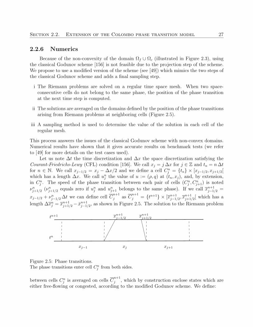
Section 2.2. Extension of the Colombo phase transition model 27
2.2.6 Numerics
Because of the non-convexity of the domain Ωf ∪ Ωc (illustrated in Figure 2.3), usingthe classical Godunov scheme [156] is not feasible due to the projection step of the scheme.We propose to use a modified version of the scheme (see [49]) which mimics the two steps ofthe classical Godunov scheme and adds a final sampling step.
i The Riemann problems are solved on a regular time space mesh. When two space-consecutive cells do not belong to the same phase, the position of the phase transitionat the next time step is computed.
ii The solutions are averaged on the domains defined by the position of the phase transitionsarising from Riemann problems at neighboring cells (Figure 2.5).
iii A sampling method is used to determine the value of the solution in each cell of theregular mesh.
This process answers the issues of the classical Godunov scheme with non-convex domains.Numerical results have shown that it gives accurate results on benchmark tests (we referto [49] for more details on the test cases used).
Let us note ∆t the time discretization and ∆x the space discretization satisfying theCourant-Friedrichs-Lewy (CFL) condition [156]. We call xj = j∆x for j ∈ Z and tn = n∆tfor n ∈ N. We call xj−1/2 = xj − ∆x/2 and we define a cell Cn
j = tn × [xj−1/2, xj+1/2[which has a length ∆x. We call unj the value of u := (ρ, q) at (tn, xj), and, by extension,in Cn
j . The speed of the phase transition between each pair of cells (Cnj , C
nj+1) is noted
νnj+1/2 (νnj+1/2 equals zero if unj and unj+1 belongs to the same phase). If we call xn+1j−1/2 =
xj−1/2 + νnj−1/2 ∆t we can define cell Cn+1
j as Cn+1
j = tn+1 × [xn+1j−1/2, x
n+1j+1/2[ which has a
length ∆xnj = xn+1j+1/2− x
n+1j−1/2, as shown in Figure 2.5. The solution to the Riemann problem
tn+1
tn
xjxj−1
xn+1j−1/2 xn+1
j+1/2
xj+1
Figure 2.5: Phase transitions.The phase transitions enter cell Cnj from both sides.
between cells Cnj is averaged on cells C
n+1
j , which by construction enclose states which areeither free-flowing or congested, according to the modified Godunov scheme. We define:
Section 2.2. Extension of the Colombo phase transition model 28
i uR(νn,+j−1/2, unj−1, u
nj ) as the solution to the Riemann problem between unj−1 and unj , at
x−xj−1/2
t−tn = νnj−1/2, and calculated at the right of the cell boundary.
ii g(νn,−j+1/2, u
nj , u
nj+1
):= f(uR(νn,−j+1/2, u
nj , u
nj+1)) with f(ρ, q) = (ρ v, q v) and the definition
of v from (2.4), as the numerical flux between cells Cnj and Cn
j+1, atx−xj+1/2
t−tn = νnj+1/2,and calculated at the left of the cell boundary.
The averaging step of the modified Godunov scheme reads:
∆xnj un+1j = ∆xunj −∆t
(g(νn,−j+1/2, u
nj , u
nj+1
)− νnj+1/2 uR
(νn,−j+1/2, u
nj , u
nj+1
))+∆t
(g(νn,+j−1/2, u
nj−1, u
nj
)− νnj−1/2 uR
(νn,+j−1/2, u
nj−1, u
nj
)).
One can notice that when there is no phase transition, νnj−1/2 = νnj+1/2 = 0, ∆x = ∆xnj andwe obtain the classical Godunov scheme. The last step is the sampling phase to define thesolutions on the cells Cn+1
j . Following [49], for cell Cn+1j we randomly pick a value between
un+1j−1 , un+1
j and un+1j+1 according to their rate of presence in cell Cn+1
j . This is done using theVan der Corput sequence (an)n∈N (2.10) which is a low-discrepancy sequence in the interval[0, 1]:
un+1j =
un+1j−1 if an ∈]0,max( ∆t
∆xnjνnj−1/2, 0)]
un+1j if an ∈] max( ∆t
∆xnjνnj−1/2, 0), 1 + min( ∆t
∆xnjνnj+1/2, 0)[
un+1j+1 if an ∈ [1 + min( ∆t
∆xnjνnj+1/2, 0), 1[
(2.10)
Remark 2.9. In the general case the congested domain Ωc is not convex in (ρ, q) coordinatesdue to the convexity of the metastable border of the domain as illustrated on Figure 2.3.It is therefore needed to add a projection step as a fourth step to the modified Godunovscheme. The projection (ρp, qp) of state (ρ, q) is defined as the solution in the metastablephase of the system:
qpρp
= qρ
vc(ρp, qp) = V
The error metric chosen to assess the numerical accuracy of the scheme is the C0(R, L1(R,R2))relative error between the computed solution and the analytical solution. We call u and ucthe exact and computed solutions respectively. For the computational domain [x0, x1] , theerror at T is computed as follows:
E(T ) =supt∈[0,T ]
∫ x1x0‖u(t, x)− uc(t, x)‖1dx
supt∈[0,T ]
∫ x1x0‖u(t, x)‖1dx
.
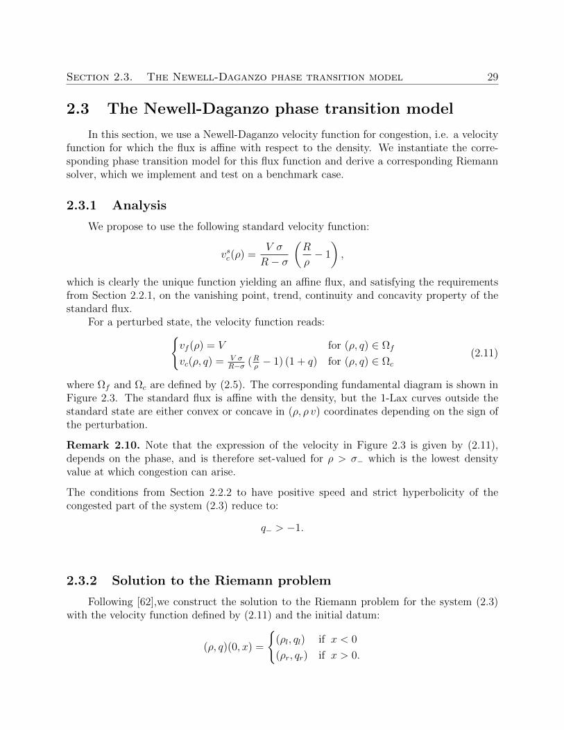
Section 2.3. The Newell-Daganzo phase transition model 29
2.3 The Newell-Daganzo phase transition model
In this section, we use a Newell-Daganzo velocity function for congestion, i.e. a velocityfunction for which the flux is affine with respect to the density. We instantiate the corre-sponding phase transition model for this flux function and derive a corresponding Riemannsolver, which we implement and test on a benchmark case.
2.3.1 Analysis
We propose to use the following standard velocity function:
vsc(ρ) =V σ
R− σ
(R
ρ− 1
),
which is clearly the unique function yielding an affine flux, and satisfying the requirementsfrom Section 2.2.1, on the vanishing point, trend, continuity and concavity property of thestandard flux.
For a perturbed state, the velocity function reads:vf (ρ) = V for (ρ, q) ∈ Ωf
vc(ρ, q) = V σR−σ (R
ρ− 1) (1 + q) for (ρ, q) ∈ Ωc
(2.11)
where Ωf and Ωc are defined by (2.5). The corresponding fundamental diagram is shown inFigure 2.3. The standard flux is affine with the density, but the 1-Lax curves outside thestandard state are either convex or concave in (ρ, ρ v) coordinates depending on the sign ofthe perturbation.
Remark 2.10. Note that the expression of the velocity in Figure 2.3 is given by (2.11),depends on the phase, and is therefore set-valued for ρ > σ− which is the lowest densityvalue at which congestion can arise.
The conditions from Section 2.2.2 to have positive speed and strict hyperbolicity of thecongested part of the system (2.3) reduce to:
q− > −1.
2.3.2 Solution to the Riemann problem
Following [62],we construct the solution to the Riemann problem for the system (2.3)with the velocity function defined by (2.11) and the initial datum:
(ρ, q)(0, x) =
(ρl, ql) if x < 0
(ρr, qr) if x > 0.
Section 2.3. The Newell-Daganzo phase transition model 30
We note u the vector (ρ, q). We define um by the solution in Ωc of the system:qmρm
= qlρl
vc(um) = vc(ur)(2.12)
which yields a quadratic polynomial in ρm. We address the general case where the solutionum of system (2.12) can coincide with ul or ur.
• Case 1: ul ∈ Ωf and ur ∈ Ωf
For all values of (ρl, ρr) the solution consists of a contact discontinuity from ul to ur.
• Case 2: ul ∈ Ωc and ur ∈ Ωc
i If ql > 0 and vc(ur) ≥ vc(ul) the solution consists of a 1-rarefaction wave from ulto um and a 2-contact discontinuity from um to ur.
ii If ql > 0 and vc(ul) > vc(ur) the solution consists of a shock wave from ul to umand a 2-contact discontinuity from um to ur.
iii If ql = 0 the solution consists of a 1-contact discontinuity from ul to um and a2-contact discontinuity from um to ur.
iv If 0 > ql and vc(ur) > vc(ul) the solution consists of a shock wave from ul to umand a 2-contact discontinuity from um to ur.
v If 0 > ql and vc(ul) ≥ vc(ur) the solution consists of a 1-rarefaction wave from ulto um and a 2-contact discontinuity from um to ur.
• Case 3: ul ∈ Ωc and ur ∈ Ωf
i If 0 > ql the solution consists of a shock wave from ul to um and of a contact-discontinuity from um to ur.
ii If ql = 0 the solution consists of a 1-contact discontinuity from ul to um and of acontact-discontinuity from um to ur.
iii If ql > 0 the solution consists of a 1-rarefaction wave from ul to um and of acontact-discontinuity from um to ur.
• Case 4: ul ∈ Ωf and ur ∈ Ωc Let um− be defined by the solution in Ωc of the system:qm−ρm−
= q−R
vc(um−) = vc(ur)
and let Λ(ul, um−) be the Rankine-Hugoniot phase transition speed between ul andum− defined by equation (2.9).
i If Λ(ul, um−) ≥ λ1(um−) the solution consists of a phase transition from ul to um−and of a 2-contact discontinuity from um− to ur.
Section 2.3. The Newell-Daganzo phase transition model 31
ii If Λ(ul, um−) < λ1(um−) let up be defined by the solution in Ωc of the system:qpρp
= q−R
Λ(ul, up) = λ1(up).
The solution consists of a phase transition from ul to up, of a 1-rarefaction wavefrom up to um−, and of a 2-contact discontinuity from um− to ur.
2.3.3 Model properties
The properties of the Newell-Daganzo model can be abstracted from the definition ofthe Riemann solver in previous Section.
The nature of the Lax curves in congestion is the same for the original Colombo modeland the Newell-Daganzo phase transition model (see Figure 2.4). Thus the solution for eachmodel differ only when a free-flow state is involved. Three differences appear in that case:
i For a given density corresponding to the free-flow phase, the associated velocity differ ingeneral between the two models.
ii Within the free-flow phase, only contact discontinuity can arise in the Newell Daganzophase transition model, whereas rarefaction waves and shockwaves can arise in the orig-inal Colombo model.
iii A transition from congestion to free-flow always involves a shock-like phase transitionin the Colombo model (and thus the solution is composed of three waves in general),whereas the transition occurs through a metastable state in the Newell-Daganzo phasetransition model, and involves only a “congestion to metastable” wave and a “metastableto free-flow” wave.
These properties are illustrated in the next Section on a Riemann problem.As in the original Colombo phase transition model [62], the 1-Lax curves are LD for q = 0,and the direction of the rarefaction waves changes according to the sign of q. This yieldsinteresting modeling capabilities, but requires the Riemann solver to be more complex thanthe one described in the following Section.
Remark 2.11. As illustrated on Figure 2.3 the flux is linear in congestion at the standardstate as per the Newell-Daganzo flux function. Remark 2.8 states that this shape modelsneutral drivers (aggressivity-wise). When the traffic is above the standard state, meaningthat the velocity is higher that what it is for the same density at the standard state, the 1-Laxcurves are concave in (ρ, ρ v) coordinates, meaning that the drivers are more aggressive. Sosuch a fundamental diagram shape seems to be in accordance with the intuition, that for agiven density, the most aggressive drivers tend to have a greater speed. This is symmetricallytrue for less aggressive drivers, also accounted for by this model.
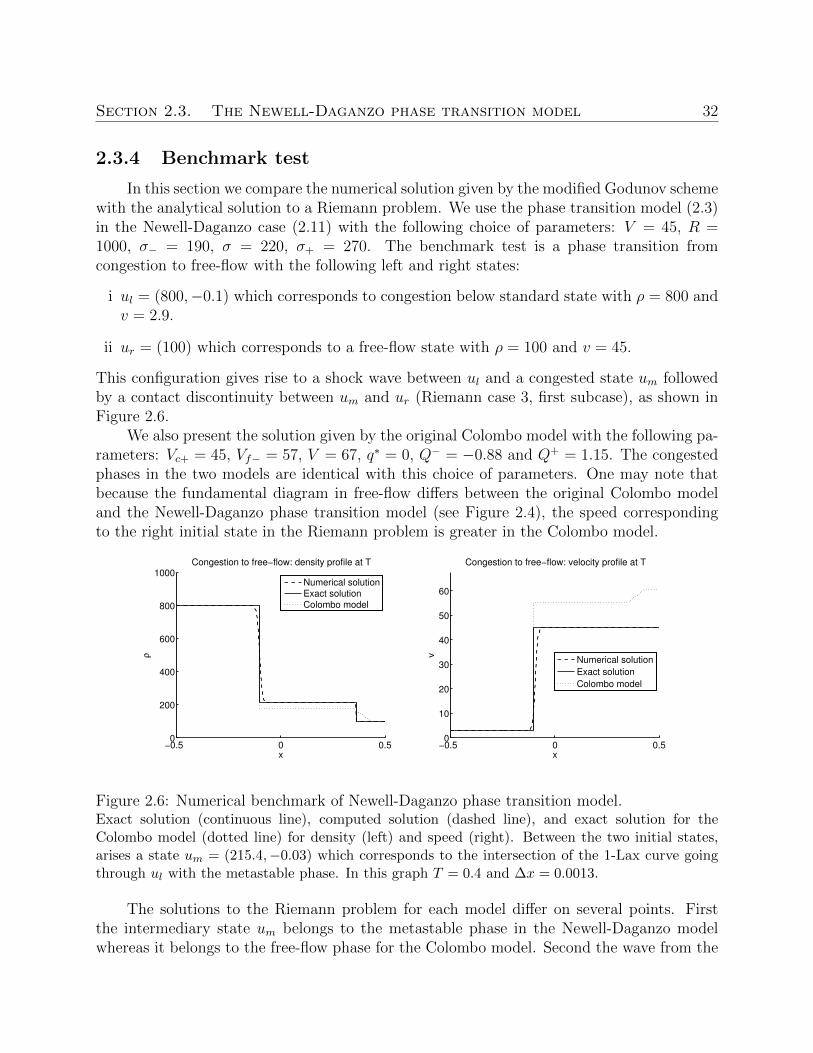
Section 2.3. The Newell-Daganzo phase transition model 32
2.3.4 Benchmark test
In this section we compare the numerical solution given by the modified Godunov schemewith the analytical solution to a Riemann problem. We use the phase transition model (2.3)in the Newell-Daganzo case (2.11) with the following choice of parameters: V = 45, R =1000, σ− = 190, σ = 220, σ+ = 270. The benchmark test is a phase transition fromcongestion to free-flow with the following left and right states:
i ul = (800,−0.1) which corresponds to congestion below standard state with ρ = 800 andv = 2.9.
ii ur = (100) which corresponds to a free-flow state with ρ = 100 and v = 45.
This configuration gives rise to a shock wave between ul and a congested state um followedby a contact discontinuity between um and ur (Riemann case 3, first subcase), as shown inFigure 2.6.
We also present the solution given by the original Colombo model with the following pa-rameters: Vc+ = 45, Vf− = 57, V = 67, q∗ = 0, Q− = −0.88 and Q+ = 1.15. The congestedphases in the two models are identical with this choice of parameters. One may note thatbecause the fundamental diagram in free-flow differs between the original Colombo modeland the Newell-Daganzo phase transition model (see Figure 2.4), the speed correspondingto the right initial state in the Riemann problem is greater in the Colombo model.
−0.5 0 0.50
200
400
600
800
1000Congestion to free−flow: density profile at T
x
ρ
−0.5 0 0.50
10
20
30
40
50
60
Congestion to free−flow: velocity profile at T
x
v
Numerical solutionExact solutionColombo model
Numerical solution
Exact solution
Colombo model
Figure 2.6: Numerical benchmark of Newell-Daganzo phase transition model.Exact solution (continuous line), computed solution (dashed line), and exact solution for theColombo model (dotted line) for density (left) and speed (right). Between the two initial states,arises a state um = (215.4,−0.03) which corresponds to the intersection of the 1-Lax curve goingthrough ul with the metastable phase. In this graph T = 0.4 and ∆x = 0.0013.
The solutions to the Riemann problem for each model differ on several points. Firstthe intermediary state um belongs to the metastable phase in the Newell-Daganzo modelwhereas it belongs to the free-flow phase for the Colombo model. Second the wave from the
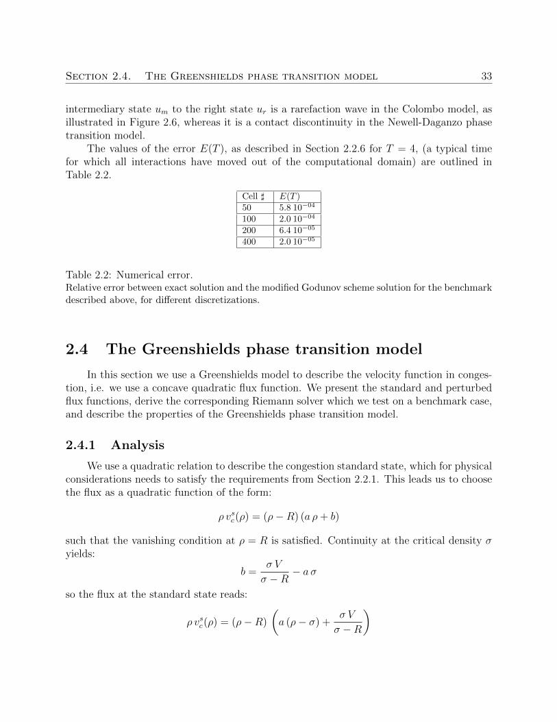
Section 2.4. The Greenshields phase transition model 33
intermediary state um to the right state ur is a rarefaction wave in the Colombo model, asillustrated in Figure 2.6, whereas it is a contact discontinuity in the Newell-Daganzo phasetransition model.
The values of the error E(T ), as described in Section 2.2.6 for T = 4, (a typical timefor which all interactions have moved out of the computational domain) are outlined inTable 2.2.
Cell ] E(T )
50 5.8 10−04
100 2.0 10−04
200 6.4 10−05
400 2.0 10−05
Table 2.2: Numerical error.Relative error between exact solution and the modified Godunov scheme solution for the benchmarkdescribed above, for different discretizations.
2.4 The Greenshields phase transition model
In this section we use a Greenshields model to describe the velocity function in conges-tion, i.e. we use a concave quadratic flux function. We present the standard and perturbedflux functions, derive the corresponding Riemann solver which we test on a benchmark case,and describe the properties of the Greenshields phase transition model.
2.4.1 Analysis
We use a quadratic relation to describe the congestion standard state, which for physicalconsiderations needs to satisfy the requirements from Section 2.2.1. This leads us to choosethe flux as a quadratic function of the form:
ρ vsc(ρ) = (ρ−R) (a ρ+ b)
such that the vanishing condition at ρ = R is satisfied. Continuity at the critical density σyields:
b =σ V
σ −R− a σ
so the flux at the standard state reads:
ρ vsc(ρ) = (ρ−R)
(a (ρ− σ) +
σ V
σ −R
)
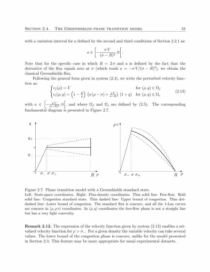
Section 2.4. The Greenshields phase transition model 34
with a variation interval for a defined by the second and third conditions of Section 2.2.1 as:
a ∈[− σ V
(σ −R)2, 0
[.
Note that for the specific case in which R = 2 σ and a is defined by the fact that thederivative of the flux equals zero at σ (which reads a = −σ V/(σ − R)2), we obtain theclassical Greenshields flux.
Following the general form given in system (2.4), we write the perturbed velocity func-tion as:
vf (ρ) = V for (ρ, q) ∈ Ωf
vc(ρ, q) =(
1− Rρ
) (a (ρ− σ) + σ V
σ−R
)(1 + q) for (ρ, q) ∈ Ωc
(2.13)
with a ∈[− σ V
(σ−R)2, 0[, and where Ωf and Ωc are defined by (2.5). The corresponding
fundamental diagram is presented in Figure 2.7.
Figure 2.7: Phase transition model with a Greenshields standard state.Left: State-space coordinates. Right: Flux-density coordinates. Thin solid line: Free-flow. Boldsolid line: Congestion standard state. Thin dashed line: Upper bound of congestion. Thin dot-dashed line: Lower bound of congestion. The standard flux is concave, and all the 1-Lax curvesare concave in (ρ, ρ v) coordinates. In (ρ, q) coordinates the free-flow phase is not a straight linebut has a very light convexity.
Remark 2.12. The expression of the velocity function given by system (2.13) enables a set-valued velocity function for ρ > σ−. For a given density the variable velocity can take severalvalues. The lower bound of the congestion phase is concave, unlike for the model presentedin Section 2.3. This feature may be more appropriate for usual experimental datasets.
Section 2.4. The Greenshields phase transition model 35
The requirements from Section 2.2.2 here reduce to:
q− > −aR
σ Vσ−R + a (2R− σ)
.
While in the Newell-Daganzo phase transition model the bound on the perturbation is givenby the fact that the speed had to be positive, here the bound is given by the requirement onthe constant concavity of the 1-Lax curves.
Remark 2.13. The lower bound on the perturbation is an increasing function of the pa-rameter a, so this parameter should be chosen as small as possible to guarantee more free-dom, namely amin = −σ V/(σ − R)2 which yields the lowest lower bound bound qmin
− =R/(2σ − 3R).
2.4.2 Solution to the Riemann problem
We consider the Riemann problem for system (2.3) with the velocity function fromequation (2.13) and the initial datum:
(ρ, q)(0, x) =
(ρl, ql) if x < 0
(ρr, qr) if x > 0.(2.14)
We follow the method used in [62] to construct the solution. We define um by the solutionin Ωc of the system:
qmρm
= qlρl
vc(um) = vc(ur)(2.15)
which yields a quadratic polynomial in ρm with one root in [0, R]. In the general case, thesolution um of the system (2.15) can be equal to ul or ur.
i Case 1:
ul ∈ Ωf and ur ∈ Ωf For all values of (ρl, ρr) the solution consists of a contact disconti-nuity from ul to ur.
ii Case 2: ul ∈ Ωc and ur ∈ Ωc
i If vc(ur) ≥ vc(ul) the solution consists of a 1-rarefaction wave from ul to um and a2-contact discontinuity from um to ur.
ii If vc(ul) > vc(ur) the solution consists of a shock wave from ul to um and a 2-contactdiscontinuity from um to ur.
iii Case 3: ul ∈ Ωc and ur ∈ Ωf The solution consists of a 1-rarefaction wave from ul toum and of a contact-discontinuity from um to ur.
Section 2.4. The Greenshields phase transition model 36
iv Case 4: ul ∈ Ωf and ur ∈ Ωc Let um− be defined by the solution in Ωc of the system:qm−ρm−
= q−R
vc(um−) = vc(ur).
The solution consists of a phase transition from ul to um− and of a 2-contact discontinuityfrom um− to ur.
Remark 2.14. The analysis in the case of a convex standard flux function, which we donot address here, is closely related to this case, modulo the sign of the parameter a and theconcavity of the 1-Lax curves.
2.4.3 Model properties
The structure of the solution to the Riemann problem presented in previous sectionexplains the distinction with the original phase transition model:
i Since the 1-Lax curves are concave, within the congestion phase, shock waves occur onlyfrom a low density on the left to a high density on the right. This is similar to classicaltraffic models with concave flux.
ii The concavity of the 1-Lax curves yields simple transitions from a free-flow state to acongested state. These phase transitions are composed of a shock-like phase transitionfollowed by a contact discontinuity, whereas a rarefaction wave can appear between thetwo in the original phase transition model or in the Newell-Daganzo phase transitionmodel.
iii Similarly to the Newell-Daganzo phase transition model, within the free-flow phase, theGreenshield phase transition model exhibits only contact discontinuities.
Another consequence of the fact that the 1-Lax curves are concave is that the Riemannsolver is much simpler than in the Newell-Daganzo case, with only five different types ofsolutions, compared to the Newell-Daganzo case which has eleven different types of solutions.
Remark 2.15. According to Remark 2.8 this flux function models aggressive drivers only,who drive along concave 1-Lax curves. In practice, it is able to model a class of clouds ofpoints observed experimentally where the congested domain has a concave lower border in(ρ, ρ v) coordinates.
2.4.4 Benchmark test
In this section we compare the numerical results given by the modified Godunov schemeon a benchmark test with its analytical solution. We use the phase transition model (2.3)
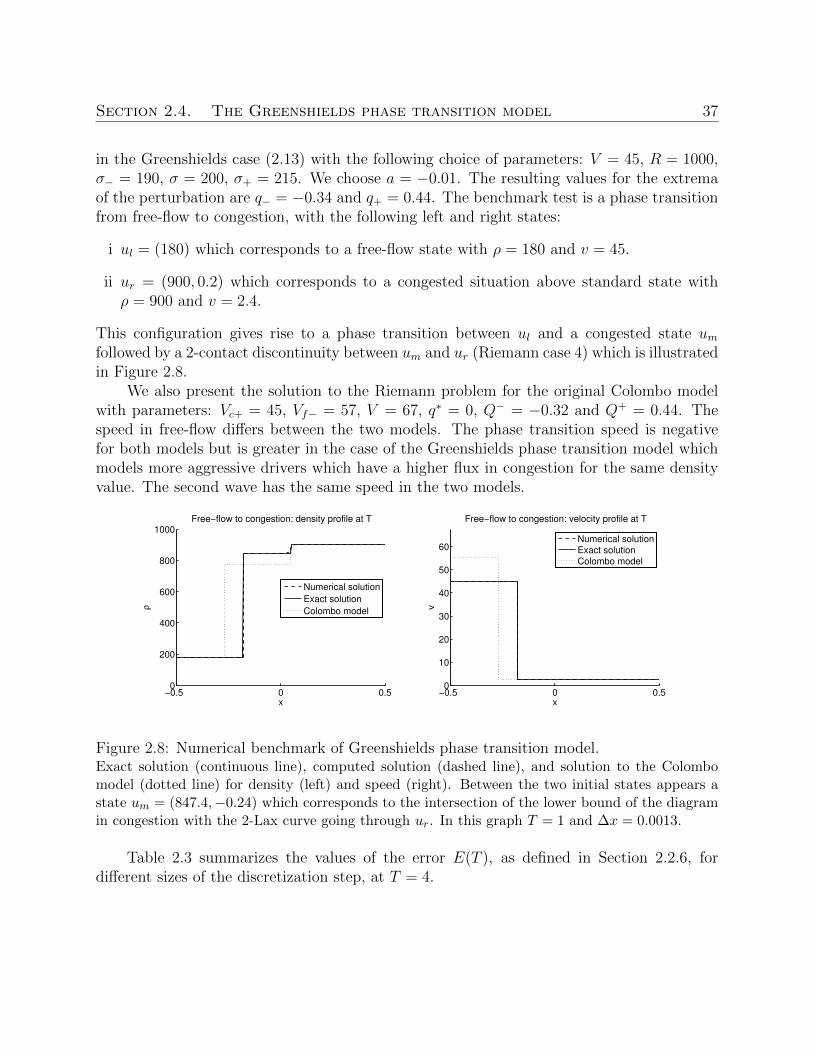
Section 2.4. The Greenshields phase transition model 37
in the Greenshields case (2.13) with the following choice of parameters: V = 45, R = 1000,σ− = 190, σ = 200, σ+ = 215. We choose a = −0.01. The resulting values for the extremaof the perturbation are q− = −0.34 and q+ = 0.44. The benchmark test is a phase transitionfrom free-flow to congestion, with the following left and right states:
i ul = (180) which corresponds to a free-flow state with ρ = 180 and v = 45.
ii ur = (900, 0.2) which corresponds to a congested situation above standard state withρ = 900 and v = 2.4.
This configuration gives rise to a phase transition between ul and a congested state umfollowed by a 2-contact discontinuity between um and ur (Riemann case 4) which is illustratedin Figure 2.8.
We also present the solution to the Riemann problem for the original Colombo modelwith parameters: Vc+ = 45, Vf− = 57, V = 67, q∗ = 0, Q− = −0.32 and Q+ = 0.44. Thespeed in free-flow differs between the two models. The phase transition speed is negativefor both models but is greater in the case of the Greenshields phase transition model whichmodels more aggressive drivers which have a higher flux in congestion for the same densityvalue. The second wave has the same speed in the two models.
−0.5 0 0.50
200
400
600
800
1000
x
ρ
Free−flow to congestion: density profile at T
−0.5 0 0.50
10
20
30
40
50
60
Free−flow to congestion: velocity profile at T
x
v
Numerical solution
Exact solution
Colombo model
Numerical solutionExact solutionColombo model
Figure 2.8: Numerical benchmark of Greenshields phase transition model.Exact solution (continuous line), computed solution (dashed line), and solution to the Colombomodel (dotted line) for density (left) and speed (right). Between the two initial states appears astate um = (847.4,−0.24) which corresponds to the intersection of the lower bound of the diagramin congestion with the 2-Lax curve going through ur. In this graph T = 1 and ∆x = 0.0013.
Table 2.3 summarizes the values of the error E(T ), as defined in Section 2.2.6, fordifferent sizes of the discretization step, at T = 4.
Section 2.5. The Li phase transition model 38
Cell ] E(T )50 3.1 10−04
100 7.8 10−05
200 2.1 10−05
400 5.4 10−06
Table 2.3: Relative error.Relative error between exact solution and numerical solution for the test case explicitly describedabove, for different numbers of space cells.
2.5 The Li phase transition model
In this section, we use a Li model [158] to describe the velocity function in congestion.The flux function is concave below a density σi in (σ,R] and is convex for densities above σi.According to our interpretation of the concavity of the flux given in remark 2.8, this modelaccounts for a changing behavior among drivers who drive in a less aggressive way whencongestion becomes too high. We present the equilibrium relation for this model, then weanalyze the perturbation, and finally we derive a Riemann solver and test it on benchmarkcases.
2.5.1 Analysis
The Li model that we use for the congestion phase is concave above critical density σuntil a density σi and is convex from σi to R. Due to the requirements listed in 2.2.1, wepropose to write the flux as a cubic function of the density.
Remark 2.16. In the following we will assume that the density parameters are sorted as0 < σ < σi ≤ R and σi ≈ R.
1. The requirement that the flux should vanish at the maximal density R leads to thefollowing expression:
ρ vsc(ρ) = (ρ−R) (a ρ2 + b ρ+ c). (2.16)
2. The existence of an inflexion point for the flux at ρ = σi yields:
d2(ρ vsc(ρ))
dρ2(σi) = 2 a (3σi −R) + 2 b = 0. (2.17)
Thus the following relation must be verified:
a =b
R− 3σi(2.18)
where we assume in agreement with remark 2.16 that R− 3σi 6= 0.
Section 2.5. The Li phase transition model 39
3. According to expression (2.17) of the second derivative of the flux and using rela-tion (2.18) between a and b, we obtain that the concavity of the flux in R is defined bythe sign of 6 b R−σi
R−3σiand assuming as per remark 2.16 that R− 3σi < 0 we must have
b < 0 to have a flux convex in R. A similar reasoning shows that the concavity of theflux in the critical density σ is defined by the sign of 6 b σ−σi
R−3σi, so in order to have a
flux concave at the critical density, assuming σ < σi consistently with remark 2.16 wemust have b < 0.
4. The continuity of the flux function at the critical density σ leads to:
c =V σ
σ −R− b
(σ2
R− 3σi+ σ
).
5. The fact that the flux is decreasing in R and in σ, and thus everywhere, comes from:
d(ρ vsc(ρ))
dρ(σ) ≤ 0 and
d(ρ vsc(ρ))
dρ(R) ≤ 0
which respectively yields:
b ≥ − σ V
(R− σ)2
R− 3σi2σ +R− 3σi
and b ≤ σ V
(R− σ)2
R− 3σi2R + σ − 3σi
where we assumed that 2 σ + R − 3σi < 0 and 2R + σ − 3σi < 0 consistently withthe ordering of the parameters of remark 2.16. The second inequality is less restrictivethan b < 0 required above.
Finally the Li flux reads:
ρ vsc(ρ) = (ρ−R)
[b
(ρ2
R− 3σi+ ρ−
(σ2
R− 3σi+ σ
))+
σ V
σ −R
](2.19)
and under this form satisfies all requirements as long as the following assumptions hold:2σ +R− 3σi < 0
b ∈[− σ V
(R−σ)2R−3σi
2σ+R−3σi, 0].
The perturbed velocity function reads:vf (ρ) = V for (ρ, q) ∈ Ωf
vc(ρ, q) =(
1− Rρ
)[a ρ2 + b ρ+ c] (1 + q) for (ρ, q) ∈ Ωc.
(2.20)
We note as in 2.2.2:
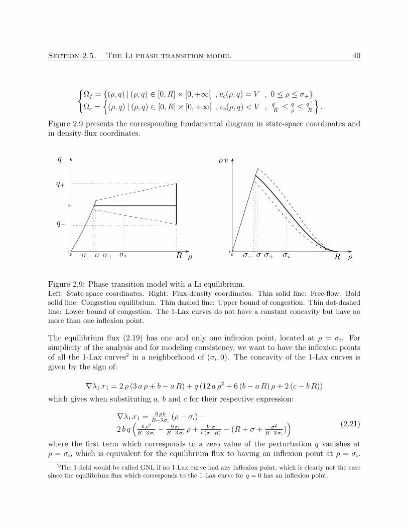
Section 2.5. The Li phase transition model 40
Ωf = (ρ, q) | (ρ, q) ∈ [0, R]× [0,+∞[ , vc(ρ, q) = V , 0 ≤ ρ ≤ σ+Ωc =
(ρ, q) | (ρ, q) ∈ [0, R]× [0,+∞[ , vc(ρ, q) < V , q−
R≤ q
ρ≤ q+
R
.
Figure 2.9 presents the corresponding fundamental diagram in state-space coordinates andin density-flux coordinates.
Figure 2.9: Phase transition model with a Li equilibrium.Left: State-space coordinates. Right: Flux-density coordinates. Thin solid line: Free-flow. Boldsolid line: Congestion equilibrium. Thin dashed line: Upper bound of congestion. Thin dot-dashedline: Lower bound of congestion. The 1-Lax curves do not have a constant concavity but have nomore than one inflexion point.
The equilibrium flux (2.19) has one and only one inflexion point, located at ρ = σi. Forsimplicity of the analysis and for modeling consistency, we want to have the inflexion pointsof all the 1-Lax curves2 in a neighborhood of (σi, 0). The concavity of the 1-Lax curves isgiven by the sign of:
∇λ1.r1 = 2 ρ (3 a ρ+ b− aR) + q (12 a ρ2 + 6 (b− aR) ρ+ 2 (c− bR))
which gives when substituting a, b and c for their respective expression:
∇λ1.r1 = 6 ρ bR−3σi
(ρ− σi)+2 b q
(6 ρ2
R−3σi− 9σi
R−3σiρ+ V σ
b (σ−R)− (R + σ + σ2
R−3σi)) (2.21)
where the first term which corresponds to a zero value of the perturbation q vanishes atρ = σi, which is equivalent for the equilibrium flux to having an inflexion point at ρ = σi.
2The 1-field would be called GNL if no 1-Lax curve had any inflexion point, which is clearly not the casesince the equilibrium flux which corresponds to the 1-Lax curve for q = 0 has an inflexion point.
Section 2.5. The Li phase transition model 41
For admissible values of b it is not possible to have expression (2.21) vanishing at (σi, q) forall q ∈ [q−, q+], thus it is not possible to have all the 1-Lax curves having an inflexion pointat ρ = σi. If we note (ρ, q) an inflexion point of a 1-Lax curve, a less restrictive conditionwould be to have its density coordinate ρ ‘close’ to the density coordinate σi of the inflexionpoint at equilibrium. In order to do so we set b such that the term which does not dependon ρ in 2.21 equals zero, i.e. b = c
Rwhich reads:
b =V σ
σ −RR− 3σi
(R− 3σi) (R + σ) + σ2
which has a sense since the denominator of the right term satisfies (R− 3σi) (R+ σ) + σ2 <(−2σ) (R+ σ) + σ2 < 0 because we assumed 2σ +R− 3σi < 0. We also proved that b < 0.We must also verify that the value chosen for b is not too small, i.e. that the flux is stilldecreasing at ρ = σ. This condition which reads:
V σ
σ −RR− 3σi
(R− 3σi) (R + σ) + σ2≥ − σ V
(R− σ)2
R− 3σi2σ +R− 3σi
is equivalent to σ− 2σi ≤ 0 which is true according to remark 2.16. Then an inflexion point(ρ, q) for a 1-Lax curve satisfies:
ρ = σi
(1 +
q
1 + 2 q
)(2.22)
where we assumed that 1 + 2 q 6= 0 (i.e. is positive given the restriction expressed by thepositivity of the speed (2.6)). In order to have the projection on the density axis of theset of inflexion points (i.e. the points (ρ, q) satisfying (2.22)) included in a neighborhood[σi (1 − α−), σi (1 + α+)]) of σi, for α−, α+ positive and small (meaning that σi (1 − α−) ≈σi ≈ σi (1 + α+)), we additionally require:
q+ ≤R
σi (1 + α+)
α+
1− 2α+
and q− ≥ −R
σi (1− α−)
α−1 + 2α−
where we assumed that α+ < 1/2 and α− < 1/2. When we add to this the conditionsfrom 2.2.2, assuming that 2R < 3σi it summarizes as:
q− ≥ max
(− R
σi (1− α−)
α−1 + 2α−
,max[σ,R]
(−
ρ d2Qeqc (ρ)dρ2
2 dQeqc (ρ)dρ
+ ρ d2Qeqc (ρ)dρ2
))and:
q+ ≤R
σi (1 + α+)
α+
1− 2α+
.
Section 2.5. The Li phase transition model 42
2.5.2 Solution of the Riemann problem
We consider the Riemann problem for system (2.3) with the velocity function definedby (2.20) and the initial datum:
(ρ, q)(0, x) =
(ρl, ql) if x < 0
(ρr, qr) if x > 0
and we follow the method used in [63] to construct the solution. We define um by the solutionin Ωc of system:
qmρm
= qlρl
vc(um) = vc(ur)
and we define up by the solution in Ωc of the system:λ1(up) = Λ(ul, up)qpρp
= qlρl.
We also note ui,l the inflexion point of the 1-Lax curve going through ul.
1. Case 1: ul ∈ Ωf and ur ∈ Ωf
For all values of (ρl, ρr) the solution consists of a contact discontinuity from ul to ur.
2. Case 2: ul ∈ Ωc and ur ∈ Ωc
(a) If vc(ul) > vc(ur) ≥ vc(ui,l) the solution consists of a shock wave from ul to umand a 2-contact discontinuity from um to ur.
(b) If vc(ur) ≥ vc(ul) ≥ vc(ui,l) the solution consists of a 1-rarefaction wave from ulto um and a 2-contact discontinuity from um to ur.
(c) If vc(ul) > vc(ui,l) > vc(ur)
i. If Λ(ul, um) ≥ λ1(um) the solution consists of a shock wave from ul to um anda 2-contact discontinuity from um to ur.
ii. If λ1(um) > Λ(ul, um) the solution consists of a shock wave from ul to up, a1-rarefaction wave from up to um and a 2-contact discontinuity from um tour.
(d) If vc(ui,l) ≥ vc(ur) > vc(ul) the solution consists of a shock wave from ul to umand a 2-contact discontinuity from um to ur.
(e) If vc(ui,l) ≥ vc(ul) ≥ vc(ur) the solution consists of a 1-rarefaction wave from ulto um and a 2-contact discontinuity from um to ur.
(f) If vc(ur) > vc(ui,l) > vc(ul)
Section 2.5. The Li phase transition model 43
i. If Λ(ul, um) ≥ λ1(um) the solution consists of a shock wave from ul to um anda 2-contact discontinuity from um to ur.
ii. If λ1(um) > Λ(ul, um) the solution consists of a shock wave from ul to up, a1-rarefaction wave from up to um and a 2-contact discontinuity from um tour.
3. Case 3: ul ∈ Ωc and ur ∈ Ωf
(a) If vc(ul) ≥ vc(ui,l) The solution consists of a 1-rarefaction wave from ul to um andof a contact-discontinuity from um to ur.
(b) If vc(ui,l) > vc(ul)
i. If Λ(ul, um) ≥ λ1(um) the solution consists of a shock wave from ul to um anda contact discontinuity from um to ur.
ii. If λ1(um) > Λ(ul, um) the solution consists of a shock wave from ul to up, a1-rarefaction wave from up to um and a contact discontinuity from um to ur.
4. Case 4: ul ∈ Ωf and ur ∈ Ωc
Let um be defined by the solution in Ωc of the system:qmρm
= q−R
vc(um) = vc(ur)
and let Λ(ul, um) be the Rankine-Hugoniot phase transition speed defined in (2.9)between ul and um.
(a) If Λ(ul, um) ≥ λ1(um) the solution consists of a phase transition from ul to umand of a 2-contact discontinuity from um to ur.
(b) If λ1(um) > Λ(ul, um) let up := (ρp, qp) be defined by the solution in Ωc of thesystem:
qpρp
= q−R
λ1(up) = Λ(ul, up).
The solution consists of a phase transition from ul to up, of a 1-rarefaction wavefrom up to um, and of a 2-contact discontinuity from um to ur.
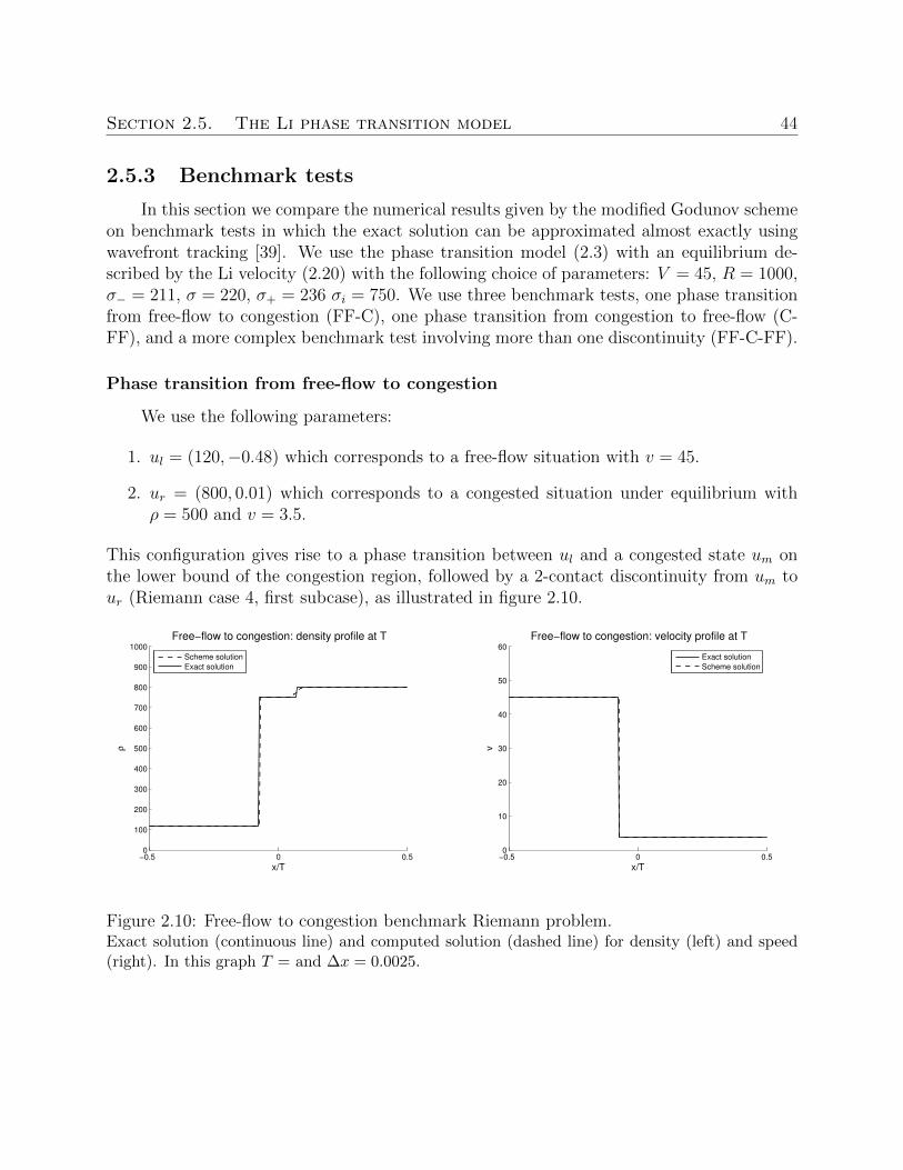
Section 2.5. The Li phase transition model 44
2.5.3 Benchmark tests
In this section we compare the numerical results given by the modified Godunov schemeon benchmark tests in which the exact solution can be approximated almost exactly usingwavefront tracking [39]. We use the phase transition model (2.3) with an equilibrium de-scribed by the Li velocity (2.20) with the following choice of parameters: V = 45, R = 1000,σ− = 211, σ = 220, σ+ = 236 σi = 750. We use three benchmark tests, one phase transitionfrom free-flow to congestion (FF-C), one phase transition from congestion to free-flow (C-FF), and a more complex benchmark test involving more than one discontinuity (FF-C-FF).
Phase transition from free-flow to congestion
We use the following parameters:
1. ul = (120,−0.48) which corresponds to a free-flow situation with v = 45.
2. ur = (800, 0.01) which corresponds to a congested situation under equilibrium withρ = 500 and v = 3.5.
This configuration gives rise to a phase transition between ul and a congested state um onthe lower bound of the congestion region, followed by a 2-contact discontinuity from um tour (Riemann case 4, first subcase), as illustrated in figure 2.10.
−0.5 0 0.50
100
200
300
400
500
600
700
800
900
1000
x/T
ρ
Free−flow to congestion: density profile at T
Scheme solution
Exact solution
−0.5 0 0.50
10
20
30
40
50
60
x/T
v
Free−flow to congestion: velocity profile at T
Exact solution
Scheme solution
Figure 2.10: Free-flow to congestion benchmark Riemann problem.Exact solution (continuous line) and computed solution (dashed line) for density (left) and speed(right). In this graph T = and ∆x = 0.0025.
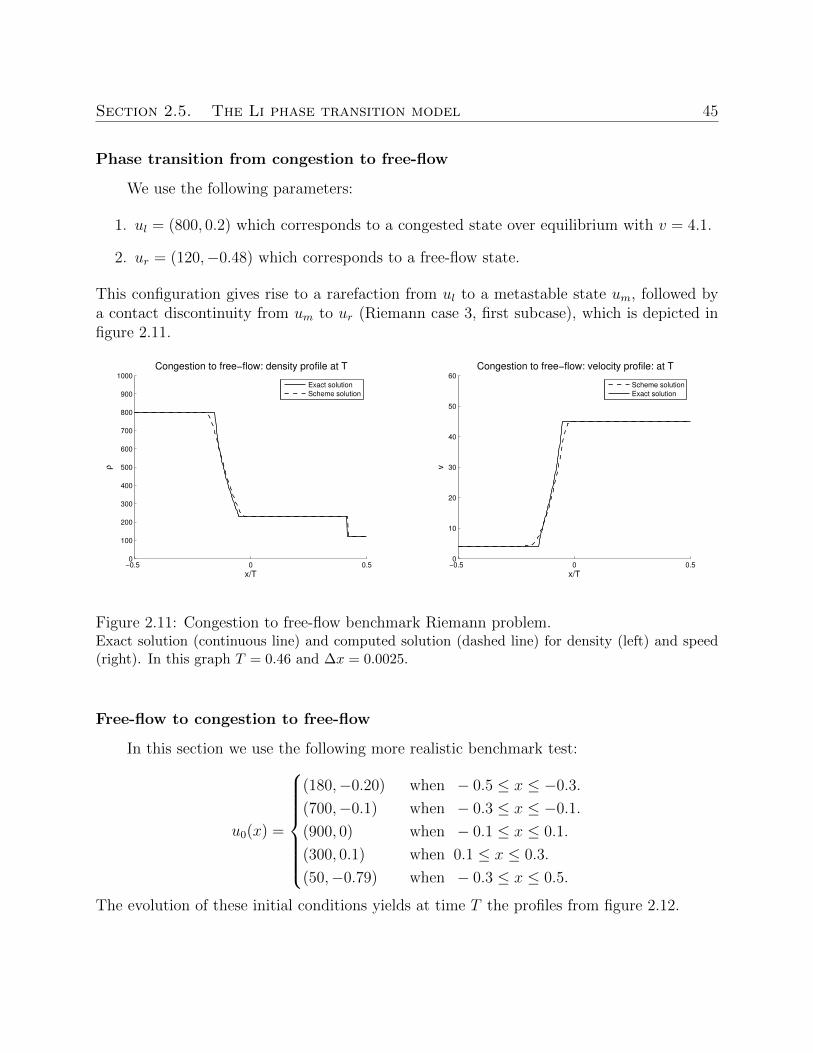
Section 2.5. The Li phase transition model 45
Phase transition from congestion to free-flow
We use the following parameters:
1. ul = (800, 0.2) which corresponds to a congested state over equilibrium with v = 4.1.
2. ur = (120,−0.48) which corresponds to a free-flow state.
This configuration gives rise to a rarefaction from ul to a metastable state um, followed bya contact discontinuity from um to ur (Riemann case 3, first subcase), which is depicted infigure 2.11.
−0.5 0 0.50
100
200
300
400
500
600
700
800
900
1000
x/T
ρ
Congestion to free−flow: density profile at T
Exact solution
Scheme solution
−0.5 0 0.50
10
20
30
40
50
60
x/T
v
Congestion to free−flow: velocity profile: at T
Scheme solution
Exact solution
Figure 2.11: Congestion to free-flow benchmark Riemann problem.Exact solution (continuous line) and computed solution (dashed line) for density (left) and speed(right). In this graph T = 0.46 and ∆x = 0.0025.
Free-flow to congestion to free-flow
In this section we use the following more realistic benchmark test:
u0(x) =
(180,−0.20) when − 0.5 ≤ x ≤ −0.3.
(700,−0.1) when − 0.3 ≤ x ≤ −0.1.
(900, 0) when − 0.1 ≤ x ≤ 0.1.
(300, 0.1) when 0.1 ≤ x ≤ 0.3.
(50,−0.79) when − 0.3 ≤ x ≤ 0.5.
The evolution of these initial conditions yields at time T the profiles from figure 2.12.
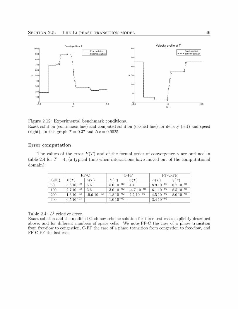
Section 2.5. The Li phase transition model 46
−0.5 0 0.50
100
200
300
400
500
600
700
800
900
1000
x/T
ρ
Density profile at T
Exact solution
Scheme solution
−0.5 0 0.50
10
20
30
40
50
60
x/T
v
Velocity profile at T
Exact solution
Scheme solution
Figure 2.12: Experimental benchmark conditions.Exact solution (continuous line) and computed solution (dashed line) for density (left) and speed(right). In this graph T = 0.37 and ∆x = 0.0025.
Error computation
The values of the error E(T ) and of the formal order of convergence γ are outlined intable 2.4 for T = 4, (a typical time when interactions have moved out of the computationaldomain).
FF-C C-FF FF-C-FFCell ] E(T ) γ(T ) E(T ) γ(T ) E(T ) γ(T )
50 5.3 10−02 6.6 5.0 10−02 4.4 8.9 10−02 8.7 10−01
100 2.7 10−02 3.6 3.0 10−02 -4.7 10−01 6.1 10−02 8.5 10−01
200 1.3 10−02 -9.6 10−02 1.8 10−02 2.2 10−02 4.5 10−02 8.0 10−01
400 6.5 10−03 1.0 10−02 3.4 10−02
Table 2.4: L1 relative error.Exact solution and the modified Godunov scheme solution for three test cases explicitly describedabove, and for different numbers of space cells. We note FF-C the case of a phase transitionfrom free-flow to congestion, C-FF the case of a phase transition from congestion to free-flow, andFF-C-FF the last case.

47
Chapter 3
Phase transition model analysis:properties and performance
In this chapter, we analyze the modeling performances of the phase transition modelintroduced in the previous chapter. After a perspective on the different scales at which trafficcan be modeled, we briefly remind the reader of the seminal scalar macroscopic traffic flowmodel described in details in Chapter 1, motivate the historical introduction of non-scalartraffic flow models, and describe how the model proposed in the previous chapter answersthe concerns and issues raised by the transportation community on so-called higher-ordermodels.
3.1 Modeling traffic at a macroscopic scale
The theory of traffic modeling incorporates the design and analysis of mathematical toolsfor accurate representation of traffic dynamics. Road networks can be studied at differentscales [155]. At a fine scale, the representation of traffic is closer to the true nature of thephenomena on the road. However, a detailed traffic model requires a large volume of accuratemeasurements for calibration and validation, and correspondingly large computation power.Consequently, different scales have been historically associated with different applications,depending on data availability and computational requirements.
At a nanoscopic scale, vehicles are considered to behave independently under the controlof a driver who reacts to stimuli from neighboring vehicles according to a specific behavioralmodel. Traffic dynamics can be modeled as a set of coupled ordinary differential equations(ODE) with decision variables resulting from a demand model (see for instance [1]). At amicroscopic scale, vehicles are considered to behave independently by reacting to stimulifrom neighboring vehicles according to a dynamical model. Traffic dynamics can be mod-eled as a set of coupled ordinary differential equations [37]. Nanoscopic and microscopicmodels have been used mostly for off-line non-real-time simulation and planning (QuadstoneParamics [45], VISSIM [94]).
Section 3.1. Modeling traffic at a macroscopic scale 48
At a mesoscopic scale, vehicles are considered as a large set of atomic elements withindividual behavior according to macroscopic laws or relations. Traffic dynamics can bemodeled as cellular automata [57] or using gas-kinetic models [188]. Mesoscopic modelshave been widely applied to real-time on-line and off-line network-wide control and dynamictraffic assignment, with significant prior data collection for calibration (DynaMIT [21], Dy-NASMART [166]).
At a macroscopic scale, vehicles are considered to behave as a continuum medium. Traf-fic dynamics is modeled as a distributed system, using partial differential equations (PDE)inspired from hydrodynamics theory [159, 97, 189]. Consequently, in this framework, theeffect of network-wide route choices is not conveniently accounted for. One of the strengthsof macroscopic models resides in the level of complexity they capture at a relatively low ana-lytical and computational cost, and with limited data requirements for calibration. This hasmotivated the use of macroscopic models in particular for real-time on-line estimation andcorridor management (METANET [168], Mobile Millennium [19], TOPL [56]). Furthermore,the mathematical theory of hydrodynamics modeling brings a solid mathematical structureto macroscopic models. This theoretical strength can be leveraged for the development ofmathematically sound lower-scale models, by equivalence (see [99, 113, 118, 155]), and serveas an anchor for the development of consistent multi-scale modeling frameworks (e.g. theAIMSUN simulation software [14]).
These properties of macroscopic models have motivated sustained research on extensionof seminal models such as the Lighthill-Whitham-Richards (LWR) model, presented in thefollowing section, with the goal of capturing complex observed phenomena missing from theLWR theory. Challenges in the design of so-called higher-order models relate to the devel-opment of sound physical understanding, well-defined analytical structure, and preservedcomputational tractability of the solution algorithm. In this chapter, we show that allowingthe speed function to take values around the classical stationary bivariate relation enablesthe simulation of higher-order traffic phenomena at the same computational cost as classicalsolution methods for the LWR model, and with a preserved physical interpretation.
In the following section, we present the historical context for the introduction of scalarmacroscopic models, presented in details in Section 1.2.3.
3.1.1 First order scalar macroscopic models
The basis for the theory of macroscopic traffic modeling was set by the seminal arti-cles from Lighthill and Whitham [159], and Richards [189], that introduced a PDE modeldescribing the evolution of the density ρ(t, x) of vehicles at time t and location x
∂ρ(t, x)
∂t+∂Q(ρ(t, x))
∂x= 0, (3.1)
where the flow is expressed as a function of the density Q(ρ(t, x)). This so-called LWR modelexpresses the conservation of vehicles on the road. Different traffic models were later shown tobe equivalent to the LWR formulation, in particular the Newell car-following model [178] and
Section 3.1. Modeling traffic at a macroscopic scale 49
the cell-transmission model (CTM) [71], in the case of a triangular flux function Q(·) [177],also called triangular fundamental diagram:
Q(ρ).=
ρ vmax if ρ ≤ ρc
(ρ− ρmax) w if ρ ≥ ρc(3.2)
where vmax, ρc, ρmax and w denote the free-flow speed, the critical density, the jam densityand the backward moving wave speed, respectively, which are required to satisfy
ρc vmax = (ρc − ρmax) w (3.3)
for continuity of the flow at the critical density. Density values below the critical densitycorrespond to free-flow states and density values above the critical density correspond tocongestion states. For non-vanishing values of the flow q and the speed v, the definition ofthe flux function Q(·) is equivalent to the definition of a speed function V (·) through theequality q = v ρ. The use of a single-valued fundamental diagram mapping a density valueto a unique flow value dates back to the observations by Greenshields in Ohio in 1934 [107],Greenberg in the Lincoln tunnel in 1959 [106], and Edie in the Holland tunnel in the early1960’s [85].
The LWR theory has been validated with experimental data for traffic modeling (see [175]for instance), and in particular the triangular fundamental diagram from equation (3.2) hasbeen shown to accurately model the stationary relation between density and flow, underproper time-space aggregation of traffic measurements [46, 47, 76]. One of the most desir-able properties of the LWR model lies in its ability to capture the formation and growthof queues at bottlenecks. However the LWR model is known to be unable to reproducemore complex observed traffic phenomena such as stop-and-go waves, traffic hysteresis, andphantom jams [118].
3.1.2 Non-stationary traffic flow
The introduction of more complex macroscopic models for traffic flow dates back tothe Payne-Whitham model (PW) [183], which consists in a 2×2 system1 of PDEs. The firstequation is the LWR PDE (see equation (3.1)) and the second equation models the accelera-tion of vehicles as resulting from a reaction to local traffic conditions and a relaxation aroundthe stationary relation. In a discrete form with a minor modification at on-ramps [182], thismodel was later used extensively for estimation and control [221, 222].
Several remarks were raised [73, 78] on the lack of physical consistency of so-calledhigher-order models, in which vehicles with negative speed, and anisotropy property, wereshown to arise. Anisotropy characterizes the fact that modeled drivers react to stimuli fromthe front and from behind2. These considerations led to the development of improved non-
1A set of 2 equations for a 2-tuple of state variables.2The justification for this terminology is the fact that in a so-called anisotropic model, we have λ1 ≤ v ≤
λ2, were v denotes the speed of vehicles, and λ1,2 the characteristic speeds at which information propagate.
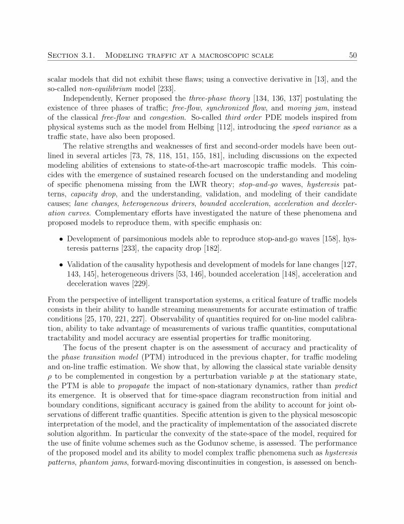
Section 3.1. Modeling traffic at a macroscopic scale 50
scalar models that did not exhibit these flaws; using a convective derivative in [13], and theso-called non-equilibrium model [233].
Independently, Kerner proposed the three-phase theory [134, 136, 137] postulating theexistence of three phases of traffic; free-flow, synchronized flow, and moving jam, insteadof the classical free-flow and congestion. So-called third order PDE models inspired fromphysical systems such as the model from Helbing [112], introducing the speed variance as atraffic state, have also been proposed.
The relative strengths and weaknesses of first and second-order models have been out-lined in several articles [73, 78, 118, 151, 155, 181], including discussions on the expectedmodeling abilities of extensions to state-of-the-art macroscopic traffic models. This coin-cides with the emergence of sustained research focused on the understanding and modelingof specific phenomena missing from the LWR theory; stop-and-go waves, hysteresis pat-terns, capacity drop, and the understanding, validation, and modeling of their candidatecauses; lane changes, heterogeneous drivers, bounded acceleration, acceleration and deceler-ation curves. Complementary efforts have investigated the nature of these phenomena andproposed models to reproduce them, with specific emphasis on:
• Development of parsimonious models able to reproduce stop-and-go waves [158], hys-teresis patterns [233], the capacity drop [182].
• Validation of the causality hypothesis and development of models for lane changes [127,143, 145], heterogeneous drivers [53, 146], bounded acceleration [148], acceleration anddeceleration waves [229].
From the perspective of intelligent transportation systems, a critical feature of traffic modelsconsists in their ability to handle streaming measurements for accurate estimation of trafficconditions [25, 170, 221, 227]. Observability of quantities required for on-line model calibra-tion, ability to take advantage of measurements of various traffic quantities, computationaltractability and model accuracy are essential properties for traffic monitoring.
The focus of the present chapter is on the assessment of accuracy and practicality ofthe phase transition model (PTM) introduced in the previous chapter, for traffic modelingand on-line traffic estimation. We show that, by allowing the classical state variable densityρ to be complemented in congestion by a perturbation variable p at the stationary state,the PTM is able to propagate the impact of non-stationary dynamics, rather than predictits emergence. It is observed that for time-space diagram reconstruction from initial andboundary conditions, significant accuracy is gained from the ability to account for joint ob-servations of different traffic quantities. Specific attention is given to the physical mesoscopicinterpretation of the model, and the practicality of implementation of the associated discretesolution algorithm. In particular the convexity of the state-space of the model, required forthe use of finite volume schemes such as the Godunov scheme, is assessed. The performanceof the proposed model and its ability to model complex traffic phenomena such as hysteresispatterns, phantom jams, forward-moving discontinuities in congestion, is assessed on bench-
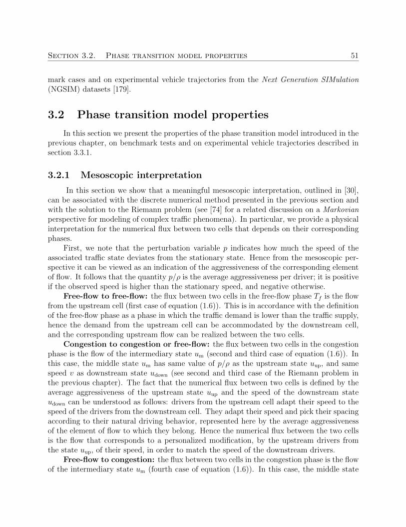
Section 3.2. Phase transition model properties 51
mark cases and on experimental vehicle trajectories from the Next Generation SIMulation(NGSIM) datasets [179].
3.2 Phase transition model properties
In this section we present the properties of the phase transition model introduced in theprevious chapter, on benchmark tests and on experimental vehicle trajectories described insection 3.3.1.
3.2.1 Mesoscopic interpretation
In this section we show that a meaningful mesoscopic interpretation, outlined in [30],can be associated with the discrete numerical method presented in the previous section andwith the solution to the Riemann problem (see [74] for a related discussion on a Markovianperspective for modeling of complex traffic phenomena). In particular, we provide a physicalinterpretation for the numerical flux between two cells that depends on their correspondingphases.
First, we note that the perturbation variable p indicates how much the speed of theassociated traffic state deviates from the stationary state. Hence from the mesoscopic per-spective it can be viewed as an indication of the aggressiveness of the corresponding elementof flow. It follows that the quantity p/ρ is the average aggressiveness per driver; it is positiveif the observed speed is higher than the stationary speed, and negative otherwise.
Free-flow to free-flow: the flux between two cells in the free-flow phase Tf is the flowfrom the upstream cell (first case of equation (1.6)). This is in accordance with the definitionof the free-flow phase as a phase in which the traffic demand is lower than the traffic supply,hence the demand from the upstream cell can be accommodated by the downstream cell,and the corresponding upstream flow can be realized between the two cells.
Congestion to congestion or free-flow: the flux between two cells in the congestionphase is the flow of the intermediary state um (second and third case of equation (1.6)). Inthis case, the middle state um has same value of p/ρ as the upstream state uup, and samespeed v as downstream state udown (see second and third case of the Riemann problem inthe previous chapter). The fact that the numerical flux between two cells is defined by theaverage aggressiveness of the upstream state uup and the speed of the downstream stateudown can be understood as follows: drivers from the upstream cell adapt their speed to thespeed of the drivers from the downstream cell. They adapt their speed and pick their spacingaccording to their natural driving behavior, represented here by the average aggressivenessof the element of flow to which they belong. Hence the numerical flux between the two cellsis the flow that corresponds to a personalized modification, by the upstream drivers fromthe state uup, of their speed, in order to match the speed of the downstream drivers.
Free-flow to congestion: the flux between two cells in the congestion phase is the flowof the intermediary state um (fourth case of equation (1.6)). In this case, the middle state
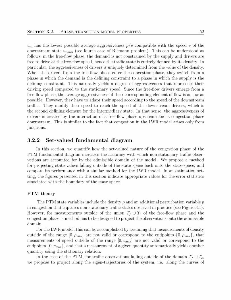
Section 3.2. Phase transition model properties 52
um has the lowest possible average aggressiveness p/ρ compatible with the speed v of thedownstream state udown (see fourth case of Riemann problem). This can be understood asfollows; in the free-flow phase, the demand is not constrained by the supply and drivers arefree to drive at the free-flow speed, hence the traffic state is entirely defined by its density. Inparticular, the aggressiveness of drivers is uniquely determined from the value of the density.When the drivers from the free-flow phase enter the congestion phase, they switch from aphase in which the demand is the defining constraint to a phase in which the supply is thedefining constraint. This naturally yields a degree of aggressiveness that represents theirdriving speed compared to the stationary speed. Since the free-flow drivers emerge from afree-flow phase, the average aggressiveness of their corresponding element of flow is as low aspossible. However, they have to adapt their speed according to the speed of the downstreamtraffic. They modify their speed to reach the speed of the downstream drivers, which isthe second defining element for the intermediary state. In that sense, the aggressiveness ofdrivers is created by the interaction of a free-flow phase upstream and a congestion phasedownstream. This is similar to the fact that congestion in the LWR model arises only fromjunctions.
3.2.2 Set-valued fundamental diagram
In this section, we quantify how the set-valued nature of the congestion phase of thePTM fundamental diagram increases the accuracy with which non-stationary traffic obser-vations are accounted for by the admissible domain of the model. We propose a methodfor projecting state values falling outside of the state space back onto the state-space, andcompare its performance with a similar method for the LWR model. In an estimation set-ting, the figures presented in this section indicate appropriate values for the error statisticsassociated with the boundary of the state-space.
PTM theory
The PTM state variables include the density ρ and an additional perturbation variable pin congestion that captures non-stationary traffic states observed in practice (see Figure 3.1).However, for measurements outside of the union Tf ∪ Tc of the free-flow phase and thecongestion phase, a method has to be designed to project the observations onto the admissibledomain.
For the LWR model, this can be accomplished by assuming that measurements of densityoutside of the range [0, ρmax] are not valid or correspond to the endpoints 0, ρmax, thatmeasurements of speed outside of the range [0, vmax] are not valid or correspond to theendpoints 0, vmax, and that a measurement of a given quantity automatically yields anotherquantity using the stationary relation.
In the case of the PTM, for traffic observations falling outside of the domain Tf ∪ Tc,we propose to project along the eigen-trajectories of the system, i.e. along the curves of
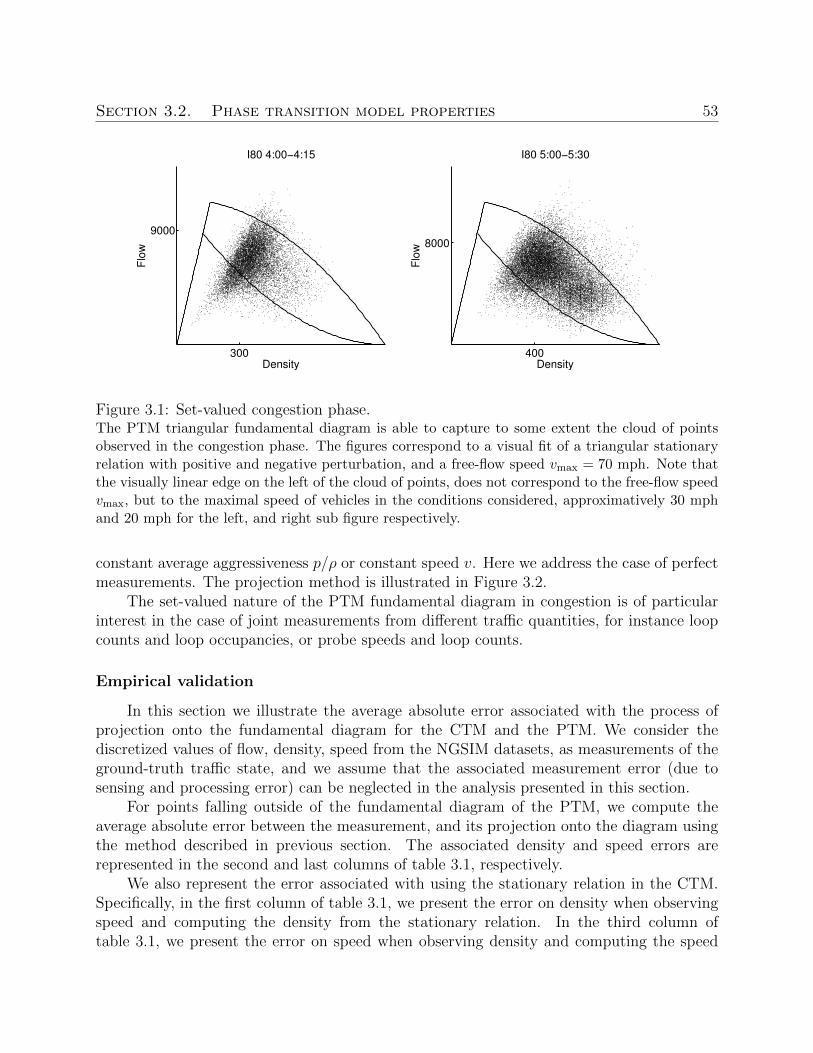
Section 3.2. Phase transition model properties 53
300
9000
Density
Flo
w
I80 4:00−4:15
400
8000
Density
Flo
w
I80 5:00−5:30
Figure 3.1: Set-valued congestion phase.The PTM triangular fundamental diagram is able to capture to some extent the cloud of pointsobserved in the congestion phase. The figures correspond to a visual fit of a triangular stationaryrelation with positive and negative perturbation, and a free-flow speed vmax = 70 mph. Note thatthe visually linear edge on the left of the cloud of points, does not correspond to the free-flow speedvmax, but to the maximal speed of vehicles in the conditions considered, approximatively 30 mphand 20 mph for the left, and right sub figure respectively.
constant average aggressiveness p/ρ or constant speed v. Here we address the case of perfectmeasurements. The projection method is illustrated in Figure 3.2.
The set-valued nature of the PTM fundamental diagram in congestion is of particularinterest in the case of joint measurements from different traffic quantities, for instance loopcounts and loop occupancies, or probe speeds and loop counts.
Empirical validation
In this section we illustrate the average absolute error associated with the process ofprojection onto the fundamental diagram for the CTM and the PTM. We consider thediscretized values of flow, density, speed from the NGSIM datasets, as measurements of theground-truth traffic state, and we assume that the associated measurement error (due tosensing and processing error) can be neglected in the analysis presented in this section.
For points falling outside of the fundamental diagram of the PTM, we compute theaverage absolute error between the measurement, and its projection onto the diagram usingthe method described in previous section. The associated density and speed errors arerepresented in the second and last columns of table 3.1, respectively.
We also represent the error associated with using the stationary relation in the CTM.Specifically, in the first column of table 3.1, we present the error on density when observingspeed and computing the density from the stationary relation. In the third column oftable 3.1, we present the error on speed when observing density and computing the speed
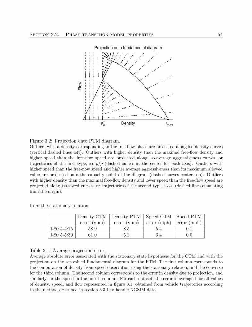
Section 3.2. Phase transition model properties 54
Density
Flo
w
Projection onto fundamental diagram
ρc
−ρ
max
Figure 3.2: Projection onto PTM diagram.Outliers with a density corresponding to the free-flow phase are projected along iso-density curves(vertical dashed lines left). Outliers with higher density than the maximal free-flow density andhigher speed than the free-flow speed are projected along iso-average aggressiveness curves, ortrajectories of the first type, iso-p/ρ (dashed curves at the center for both axis). Outliers withhigher speed than the free-flow speed and higher average aggressiveness than its maximum allowedvalue are projected onto the capacity point of the diagram (dashed curves center top). Outlierswith higher density than the maximal free-flow density and lower speed than the free-flow speed areprojected along iso-speed curves, or trajectories of the second type, iso-v (dashed lines emanatingfrom the origin).
from the stationary relation.
Density CTM Density PTM Speed CTM Speed PTMerror (vpm) error (vpm) error (mph) error (mph)
I-80 4-4:15 58.9 8.5 5.4 0.1I-80 5-5:30 61.0 5.2 3.4 0.0
Table 3.1: Average projection error.Average absolute error associated with the stationary state hypothesis for the CTM and with theprojection on the set-valued fundamental diagram for the PTM. The first column corresponds tothe computation of density from speed observation using the stationary relation, and the conversefor the third column. The second column corresponds to the error in density due to projection, andsimilarly for the speed in the fourth column. For each dataset, the error is averaged for all valuesof density, speed, and flow represented in figure 3.1, obtained from vehicle trajectories accordingto the method described in section 3.3.1 to handle NGSIM data.
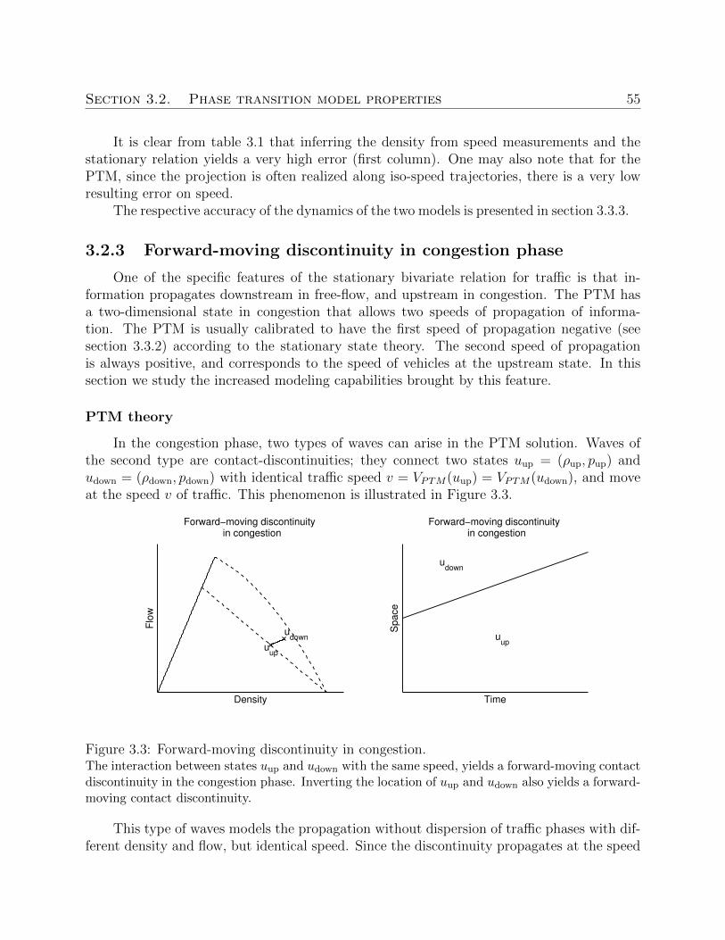
Section 3.2. Phase transition model properties 55
It is clear from table 3.1 that inferring the density from speed measurements and thestationary relation yields a very high error (first column). One may also note that for thePTM, since the projection is often realized along iso-speed trajectories, there is a very lowresulting error on speed.
The respective accuracy of the dynamics of the two models is presented in section 3.3.3.
3.2.3 Forward-moving discontinuity in congestion phase
One of the specific features of the stationary bivariate relation for traffic is that in-formation propagates downstream in free-flow, and upstream in congestion. The PTM hasa two-dimensional state in congestion that allows two speeds of propagation of informa-tion. The PTM is usually calibrated to have the first speed of propagation negative (seesection 3.3.2) according to the stationary state theory. The second speed of propagationis always positive, and corresponds to the speed of vehicles at the upstream state. In thissection we study the increased modeling capabilities brought by this feature.
PTM theory
In the congestion phase, two types of waves can arise in the PTM solution. Waves ofthe second type are contact-discontinuities; they connect two states uup = (ρup, pup) andudown = (ρdown, pdown) with identical traffic speed v = VPTM(uup) = VPTM(udown), and moveat the speed v of traffic. This phenomenon is illustrated in Figure 3.3.
udown
uup
Density
Flo
w
Forward−moving discontinuity in congestion
uup
udown
Time
Sp
ace
Forward−moving discontinuity in congestion
Figure 3.3: Forward-moving discontinuity in congestion.The interaction between states uup and udown with the same speed, yields a forward-moving contactdiscontinuity in the congestion phase. Inverting the location of uup and udown also yields a forward-moving contact discontinuity.
This type of waves models the propagation without dispersion of traffic phases with dif-ferent density and flow, but identical speed. Since the discontinuity propagates at the speed
Section 3.2. Phase transition model properties 56
of traffic, this phenomenon does not depend on the sign of the flow difference between theupstream and the downstream phase, and, unlike for a shockwave, no mixing is introducedbetween the two states on each side of the discontinuity. The interface between two groupsof vehicles with different densities and flow but identical speed is preserved with time.
Empirical validation
The aggregate time-space diagrams for density and speed in the I80 5-5:30 dataset arepresented in Figure 3.4.
In addition to several backward moving shock waves spanning the entire domain, weobserve a clear forward-moving discontinuity emanating from the upstream of the sectionaround time 750 seconds. A number of forward-moving discontinuities are observed duringthe episodes of light congestion (blue in figure 3.4). One may note that the forward-movingdiscontinuities for the episodes of light congestion travel faster than the forward moving dis-continuity corresponding to heavy congestion (red in figure 3.4), as the PTM would predict.Finally the comparison of the top and bottom plots of Figure 3.4 illustrates that discon-tinuities in density can propagate forward or backward, whereas discontinuities in speedonly propagate backward, which corresponds to the constitutive properties of the PTM. Theability of the model to reproduce this phenomenon is illustrated in section 3.3.3.
3.2.4 Hysteresis phenomenon
The phenomenon of hysteresis has been studied with much attention by the trans-portation community [176, 214, 232], with different candidate explanations; acceleration anddeceleration waves, heterogeneous drivers, lane changes. Recent results [144] seem to discardthe hypothesis of acceleration and deceleration waves in favor of the hypothesis of heteroge-neous drivers. The model proposed is consistent with this theory in the sense that loops canform in both directions, irrespective of the speed gradient.
The existence of hysteresis loops in density-flow coordinates can be traced back tothe solution to the Riemann problem (second case of uup, udown, in the congestion phaseTc). An intermediary state um arises between the initial upstream state uup and the initialdownstream state udown. The upstream state uup and the intermediary state um have thesame value of the average aggressiveness per driver p/ρ. The downstream state udown andthe intermediary state um have the same value of speed v. The relative value of these twoquantities for the upstream and downstream states uup and udown impacts the orientation ofthe loop (see Figure 3.5).
Only two configurations are possible in congestion for which no hysteresis loop arises.
• In the case of an upstream state uup and a downstream state udown with the samevalue of the average aggressiveness p/ρ, no hysteresis occurs, and the only differenceintroduced by switching the two states is the change of nature of the connecting wave(shock or rarefaction).
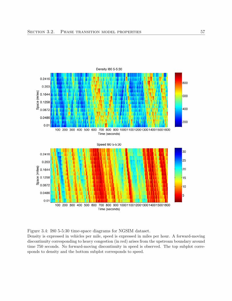
Section 3.2. Phase transition model properties 57
Figure 3.4: I80 5-5:30 time-space diagrams for NGSIM dataset.Density is expressed in vehicles per mile, speed is expressed in miles per hour. A forward-movingdiscontinuity corresponding to heavy congestion (in red) arises from the upstream boundary aroundtime 750 seconds. No forward-moving discontinuity in speed is observed. The top subplot corre-sponds to density and the bottom subplot corresponds to speed.
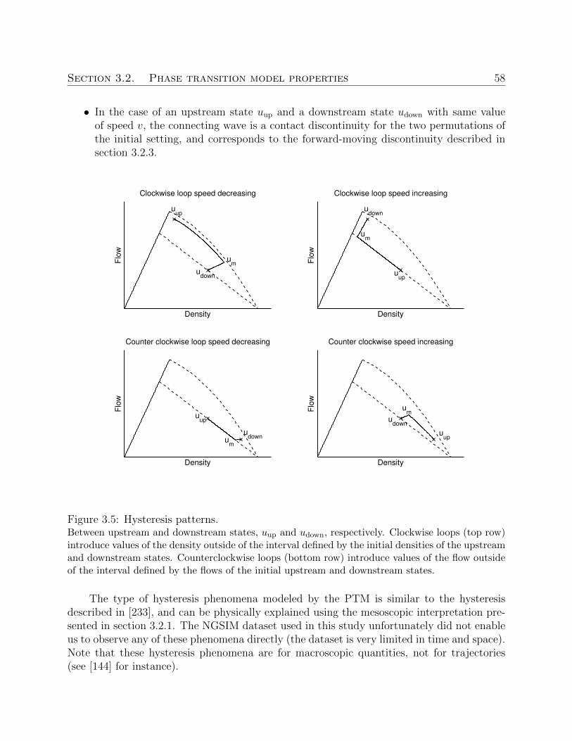
Section 3.2. Phase transition model properties 58
• In the case of an upstream state uup and a downstream state udown with same valueof speed v, the connecting wave is a contact discontinuity for the two permutations ofthe initial setting, and corresponds to the forward-moving discontinuity described insection 3.2.3.
uup
udown
um
Density
Flo
w
Clockwise loop speed decreasing
udown
uup
um
DensityF
low
Clockwise loop speed increasing
uup
udown
um
Density
Flo
w
Counter clockwise speed increasing
udown
uup
um
Density
Flo
w
Counter clockwise loop speed decreasing
Figure 3.5: Hysteresis patterns.Between upstream and downstream states, uup and udown, respectively. Clockwise loops (top row)introduce values of the density outside of the interval defined by the initial densities of the upstreamand downstream states. Counterclockwise loops (bottom row) introduce values of the flow outsideof the interval defined by the flows of the initial upstream and downstream states.
The type of hysteresis phenomena modeled by the PTM is similar to the hysteresisdescribed in [233], and can be physically explained using the mesoscopic interpretation pre-sented in section 3.2.1. The NGSIM dataset used in this study unfortunately did not enableus to observe any of these phenomena directly (the dataset is very limited in time and space).Note that these hysteresis phenomena are for macroscopic quantities, not for trajectories(see [144] for instance).
Section 3.2. Phase transition model properties 59
3.2.5 Phantom jam
The emergence and propagation of traffic disturbances causing drivers to decrease theirspeed for no clear reason in congestion, or so-called phantom jams, is well-known to mostcommuters and the topic of active research, with recent explanations tracing its cause backto the heterogeneity of driving behaviors [146]. It is clear from the solution to the Riemannproblem that the PTM is not able to model the emergence of extreme3 values of speed.However, in this section we show that the PTM is able to model the emergence of extremevalues of density and flow.
We motivate the subsequent macroscopic description by the mesoscopic model describedin section 3.2.1, in which drivers from an upstream phase adjust their speed to the speedof the drivers from the downstream phase, according to their own driving behavior. Onemight note that this mesoscopic model can be obtained similarly by expressing the fact thatupstream drivers maximize their speed under the constraint of their driving behavior, andthe speed of the downstream drivers, that they cannot exceed without creating an accident.
In the congestion phase, the solution to the Riemann problem associated with the PTMexhibits different types of hysteresis loops (see previous section). It is clear that the interme-diary state arising always has a speed in the interval defined by the speeds of the upstreamand downstream states. However, different loop behaviors can arise (see Figure 3.5):
1. Clockwise loops are the cause of the emergence of intermediary states with extremevalues of density (top row). In the case of a transition from a high speed to a lowspeed, a higher value of density arises (top left case) whereas in the case of a transitionfrom a low speed to a high speed a lower value of density arises (top right case).
2. Counter-clockwise loops are the cause of the emergence of intermediary states withextreme values of flow (bottom row). In the case of a transition from a high speedto a low speed, a lower value of flow arises (bottom left case) whereas in the case ofa transition from a low speed to a high speed a higher value of flow arises (top rightcase).
In the four cases described above, from a mesoscopic perspective, the difference inflow and density between the downstream state udown and the middle emerging state um
is explained by the fact that the upstream and downstream drivers have different levels ofaggressiveness, translating into different preferred spacing for the same speed.
This feature of the PTM seems appropriate for modeling the propagation of disturbancesin traffic. In Figure 3.5, one can note that if udown is viewed as a disturbance of uup, then theintermediary state um arising is always an amplified disturbance, in density or flow, and thisamplified disturbance travels upstream (negative wave speed connecting uup and um). Notethat this phenomenon is a locally convected phenomenon, i.e. it results from the emergenceof um from uup and udown. It is very different from convective instabilities commonly observedin fluids, characterized by a dispersion relation [190], that amplify over time.
3In the context of a Riemann problem, by extreme value of speed we mean a value of speed outside ofthe interval defined by the speeds of the upstream and downstream states.
Section 3.3. Phase transition model validation 60
3.3 Phase transition model validation
In this section we present the datasets and the numerical methods used in the followingmodel calibration and model comparison.
3.3.1 Vehicle trajectories datasets
Datasets specifications
We consider the following NGSIM datasets [179] from highway I-80:
1. I-80 4:00-4:15: vehicles trajectories are recorded at a 0.1 second resolution for a 0.34miles stretch of freeway I-80 Northbound at Powell Street, Emeryville, CA, with 6lanes including a HOV lane, during 15 minutes from 4 pm to 4:15 pm (2052 vehicles).We consider the middle stretch from relative mile 0.03 to relative mile 0.3, which is astraight line. We remove the first and last 100 seconds to avoid boundary effects. Wediscretize the dataset into 14 cells and 749 time-steps.
2. I-80 5:00-5:30: vehicles trajectories are recorded at a 0.1 second resolution for a 0.34miles stretch of freeway I-80 Northbound at Powell Street, Emeryville, CA, with 6lanes including a HOV lane, during 30 minutes from 5 pm to 5:30 pm (3626 vehicles).We consider the middle stretch from relative mile 0.03 to relative mile 0.3, which is astraight line. We remove the first 100 and last 250 seconds to avoid boundary effect.We discretize the dataset into 14 cells and 1104 time-steps.
The choice of the number of cells for discretization of the dataset is driven by the samplingfrequency of the collected data for accurate computation of flow, density and speed accordingto Edie’s generalized definition [84]. We want to have a time-step “large” compared to thesampling period and a cell size “large” compared to the distance traveled by the vehiclesduring a sampling period (see [155] for a detailed discussion on the notion of scale in trafficmodeling). Here we consider a time-step of 10 times the sampling period, and a cell-size of 10times the distance traveled at the free-flow speed (taken as 70 mph) between two consecutivereports. The average point speed of the vehicles is 17 mph and 12 mph for I-80 4:00-4:15and I-80 5:00-5:30, respectively. The discretization parameters for each dataset are given intable 3.2.
Sampling period Time-step Cell size Average ] pointsper cell
I-80 4-4:15 0.1 sec 1 sec 102 feet 71 pointsI-80 5-5:30 0.1 sec 1 sec 102 feet 96 points
Table 3.2: Discretization parameters for NGSIM dataset.The time-step and cell-size are chosen as a function of the sampling period.
Section 3.3. Phase transition model validation 61
In the following analysis, we consider the computed values of density, flow and speedaccording to Edie’s generalized definition, for the discretization grid associated with theparameters from table 3.2, as ground-truth traffic state for benchmarking the performancesof the PTM and the CTM.
Dataset properties
The density time-space diagrams of the NGSIM datasets used for model testing andvalidation are reproduced in Figure 3.6. In this figure, the 5 leftmost mainline lanes areconsidered for computation of the density, flow, and speed according to Edie’s generalizeddefinition, with discretization parameters described in previous sub section.
The dataset consists of 5 mainline lanes including an HOV lane, with an on-rampupstream of the stretch considered and an off-ramp downstream. Several heavy congestionpatterns can be observed propagating upstream at similar speeds. Heavy congestion can alsobe observed propagating downstream in the I80 5-5:30 dataset, starting from the upstreamboundary at around 800 seconds in relative time. Several light congestion waves can alsobe observed propagating downstream, starting from downstream of heavy congestion, in thelast quarter of the I80 4-4:15 dataset.
One may note that the datasets considered exhibit only congestion phenomena, henceonly allow the validation of the PTM in the congestion phase. This is a clear limitation ofthe experimental results presented here, that should be complemented in the future by ananalysis of the performance of the PTM on datasets more representative of general trafficproperties.
In the following section, we present a method for calibrating the parameters of the PTM,and the results obtained on the datasets described in this section.
3.3.2 Model calibration
The parameters of the PTM consist of the free-flow speed, the parameters of thestationary relation used in the congestion phase, and the parameters pmin and pmax, specifyingthe maximal admissible range around the stationary relation for the fundamental diagramin congestion.
Several algorithms can be found in the literature for calibration of a single model pa-rameter, in particular in the case of the CTM. The jam density ρmax and the free-flow speedvmax are usually assumed to be known, and the congestion wave speed w can be estimated us-ing different methods. An algorithm for the estimation of the congestion wave speed basedon vehicle trajectories can be found in [164]. This parameter can similarly be estimatedconsidering a Lagrangian approach as described in [52].
In this section, we consider a methodology similar to the methodology described in [67],for joint estimation of all parameters of the model from macroscopic quantities.
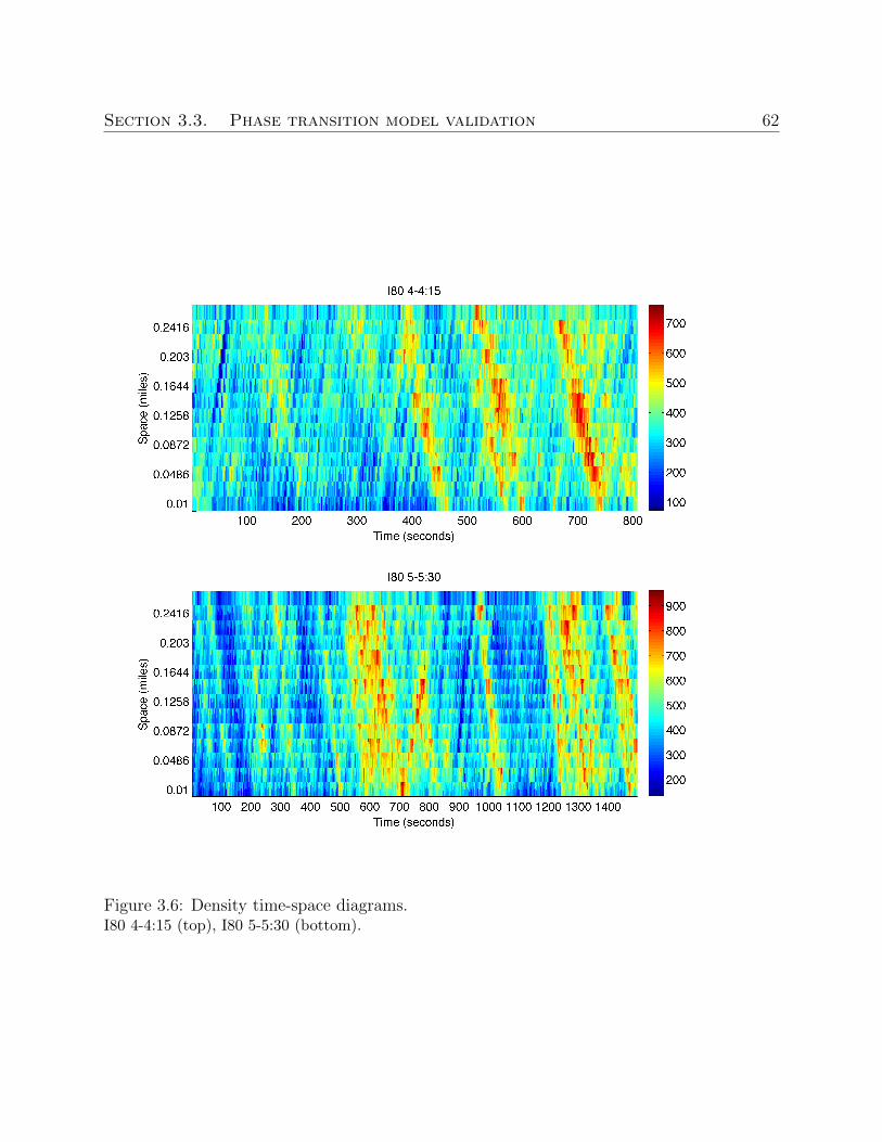
Section 3.3. Phase transition model validation 62
Figure 3.6: Density time-space diagrams.I80 4-4:15 (top), I80 5-5:30 (bottom).
Section 3.3. Phase transition model validation 63
Methodology and results
We propose to compare the time space diagrams reconstructed by the PTM and theCTM from the knowledge of initial and boundary conditions. Given a training data setof macroscopic measurements, the method consists of the definition of a cost function, thedirect computation of the initial and boundary condition, and of the identification of the setof parameters at which the minimum of the cost function is attained for the reconstructedtime space diagrams. We consider the L1 metric:
L1(uPTM) =
∑n
∑j |uPTM(n∆t, j∆x)− uNGSIM(n∆t, j∆x)|∑
n
∑j |uNGSIM(n∆t, j∆x)|
, (3.4)
in which we note uPTM(n∆t, j∆x) the value of the quantity u, at the cell indexed by n, atthe time-step indexed by j, computed using the discrete PTM on a grid with discretizationparameters ∆t and ∆x. We use a similar notation for the ground-truth uNGSIM obtainedby discretizing the NGSIM vehicle trajectories.
The quantities uNGSIM and uPTM must be defined on the same discretization grid.The reference uNGSIM is defined on the physical grid described in section 3.3.1, chosenaccording to data availability. The discrete solution uPTM to the PTM can be computed onan arbitrarily refined numerical grid. The discrete solution converges toward the analyticalsolution when the refinement of the numerical grid increases. The level of refinement ofthe grid is guided by the numerical benchmarks from [31] and [49], which provide empiricalresults on the distance to the analytical solution of the PDE as a function of the refinementlevel. The values of the reference uNGSIM on the refined grid can be obtained from its valueson the coarse physical grid in a straightforward manner.
In order to assess the importance of the error variable used for calibration, we proposeto compute the error metric (3.4) where u is successively defined as ρ, q and v. Due to thenonlinearity of the models investigated, and the consequent non-convexity of the optimizationproblem considered, the cost function is optimized by exhaustive enumeration on a a gridwith parameters ∆ρ = 10 vpm, ∆v = 5 mph, ∆w = 0.5 mph, ∆pmin = 0.1, ∆pmax = 0.1.The optimal parameters for I80 4:00-4:15 and I80 5:00-5:30 are presented in tables 3.3 and 3.4respectively. In the interest of space, we only consider the instantiation of the PTM for atriangular stationary relation, with potentially positive and negative perturbation.
The optimal parameters obtained fall into the range of plausible values from a physicalperspective. There is significant dependency of the optimal parameters to the error variable(which arises for the CTM as well, but is not represented here, in the interest of space).One might note that the optimal value of the congestion wave speed obtained for the 5aggregated lanes is greater than the typical value for a single lane (around 11.5 mph), whichmight be due to tentative lane changes. The optimal value of the congestion wave speed isfairly stable across error variables, however the jam density exhibits large relative variations,in particular for the I80 datasets in which the congestion level is more important.
The optimal parameters obtained for different error variables can vary significantly for agiven dataset, in particular for the perturbation parameters. In the case of the density error
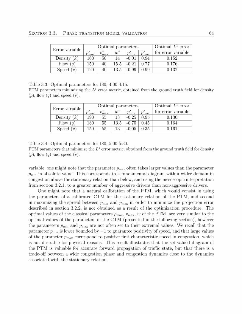
Section 3.3. Phase transition model validation 64
Error variableOptimal parameters Optimal L1 error
ρ∗max v∗max w∗ p∗min p∗max for error variableDensity (k) 160 50 14 -0.01 0.94 0.152
Flow (q) 150 40 15.5 -0.21 0.77 0.176Speed (v) 120 40 13.5 -0.99 0.99 0.137
Table 3.3: Optimal parameters for I80, 4:00-4:15.PTM parameters minimizing the L1 error metric, obtained from the ground truth field for density(ρ), flow (q) and speed (v).
Error variableOptimal parameters Optimal L1 error
ρ∗max v∗max w∗ p∗min p∗max for error variableDensity (k) 190 55 13 -0.25 0.95 0.130
Flow (q) 180 55 13.5 -0.75 0.45 0.164Speed (v) 150 55 13 -0.05 0.35 0.161
Table 3.4: Optimal parameters for I80, 5:00-5:30.PTM parameters that minimize the L1 error metric, obtained from the ground truth field for density(ρ), flow (q) and speed (v).
variable, one might note that the parameter pmax often takes larger values than the parameterpmin in absolute value. This corresponds to a fundamental diagram with a wider domain incongestion above the stationary relation than below, and using the mesoscopic interpretationfrom section 3.2.1, to a greater number of aggressive drivers than non-aggressive drivers.
One might note that a natural calibration of the PTM, which would consist in usingthe parameters of a calibrated CTM for the stationary relation of the PTM, and secondin maximizing the spread between pmin and pmax in order to minimize the projection errordescribed in section 3.2.2, is not obtained as a result of the optimization procedure. Theoptimal values of the classical parameters ρmax, vmax, w of the PTM, are very similar to theoptimal values of the parameters of the CTM (presented in the following section), howeverthe parameters pmin and pmax are not often set to their extremal values. We recall that theparameter pmin is lower bounded by −1 to guarantee positivity of speed, and that large valuesof the parameter pmax correspond to positive first characteristic speed in congestion, whichis not desirable for physical reasons. This result illustrates that the set-valued diagram ofthe PTM is valuable for accurate forward propagation of traffic state, but that there is atrade-off between a wide congestion phase and congestion dynamics close to the dynamicsassociated with the stationary relation.
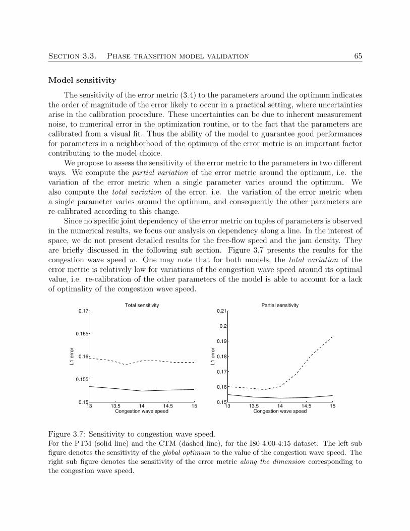
Section 3.3. Phase transition model validation 65
Model sensitivity
The sensitivity of the error metric (3.4) to the parameters around the optimum indicatesthe order of magnitude of the error likely to occur in a practical setting, where uncertaintiesarise in the calibration procedure. These uncertainties can be due to inherent measurementnoise, to numerical error in the optimization routine, or to the fact that the parameters arecalibrated from a visual fit. Thus the ability of the model to guarantee good performancesfor parameters in a neighborhood of the optimum of the error metric is an important factorcontributing to the model choice.
We propose to assess the sensitivity of the error metric to the parameters in two differentways. We compute the partial variation of the error metric around the optimum, i.e. thevariation of the error metric when a single parameter varies around the optimum. Wealso compute the total variation of the error, i.e. the variation of the error metric whena single parameter varies around the optimum, and consequently the other parameters arere-calibrated according to this change.
Since no specific joint dependency of the error metric on tuples of parameters is observedin the numerical results, we focus our analysis on dependency along a line. In the interest ofspace, we do not present detailed results for the free-flow speed and the jam density. Theyare briefly discussed in the following sub section. Figure 3.7 presents the results for thecongestion wave speed w. One may note that for both models, the total variation of theerror metric is relatively low for variations of the congestion wave speed around its optimalvalue, i.e. re-calibration of the other parameters of the model is able to account for a lackof optimality of the congestion wave speed.
13 13.5 14 14.5 150.15
0.16
0.17
0.18
0.19
0.2
0.21
Congestion wave speed
L1
err
or
Partial sensitivity
13 13.5 14 14.5 150.15
0.155
0.16
0.165
0.17
Congestion wave speed
L1
err
or
Total sensitivity
Figure 3.7: Sensitivity to congestion wave speed.For the PTM (solid line) and the CTM (dashed line), for the I80 4:00-4:15 dataset. The left subfigure denotes the sensitivity of the global optimum to the value of the congestion wave speed. Theright sub figure denotes the sensitivity of the error metric along the dimension corresponding tothe congestion wave speed.
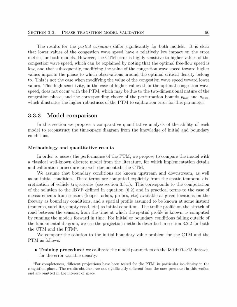
Section 3.3. Phase transition model validation 66
The results for the partial variation differ significantly for both models. It is clearthat lower values of the congestion wave speed have a relatively low impact on the errormetric, for both models. However, the CTM error is highly sensitive to higher values of thecongestion wave speed, which can be explained by noting that the optimal free-flow speed islow, and that subsequently, modifying the value of the congestion wave speed toward highervalues impacts the phase to which observations around the optimal critical density belongto. This is not the case when modifying the value of the congestion wave speed toward lowervalues. This high sensitivity, in the case of higher values than the optimal congestion wavespeed, does not occur with the PTM, which may be due to the two-dimensional nature of thecongestion phase, and the corresponding choice of the perturbation bounds pmin and pmax,which illustrates the higher robustness of the PTM to calibration error for this parameter.
3.3.3 Model comparison
In this section we propose a comparative quantitative analysis of the ability of eachmodel to reconstruct the time-space diagram from the knowledge of initial and boundaryconditions.
Methodology and quantitative results
In order to assess the performance of the PTM, we propose to compare the model witha classical well-known discrete model from the literature, for which implementation detailsand calibration procedure are well documented: the CTM.
We assume that boundary conditions are known upstream and downstream, as wellas an initial condition. These terms are computed explicitly from the spatio-temporal dis-cretization of vehicle trajectories (see section 3.3.1). This corresponds to the computationof the solution to the IBVP defined in equation (6.2) and in practical terms to the case ofmeasurements from sensors (loops, radars, probes, etc) available at given locations on thefreeway as boundary conditions, and a spatial profile assumed to be known at some instant(cameras, satellite, empty road, etc) as initial condition. The traffic profile on the stretch ofroad between the sensors, from the time at which the spatial profile is known, is computedby running the models forward in time. For initial or boundary conditions falling outside ofthe fundamental diagram, we use the projection methods described in section 3.2.2 for boththe CTM and the PTM4.
We compare the solution to the initial-boundary value problem for the CTM and thePTM as follows:
• Training procedure: we calibrate the model parameters on the I80 4:00-4:15 dataset,for the error variable density.
4For completeness, different projections have been tested for the PTM, in particular iso-density in thecongestion phase. The results obtained are not significantly different from the ones presented in this sectionand are omitted in the interest of space.
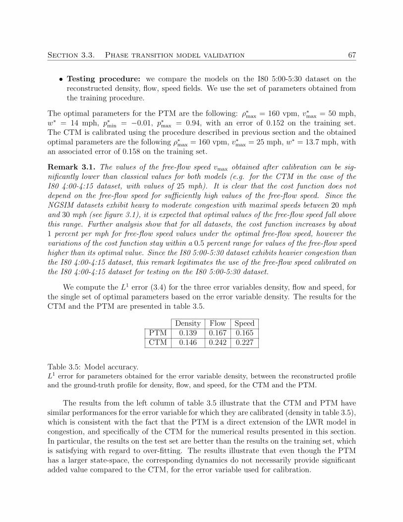
Section 3.3. Phase transition model validation 67
• Testing procedure: we compare the models on the I80 5:00-5:30 dataset on thereconstructed density, flow, speed fields. We use the set of parameters obtained fromthe training procedure.
The optimal parameters for the PTM are the following: ρ∗max = 160 vpm, v∗max = 50 mph,w∗ = 14 mph, p∗min = −0.01, p∗max = 0.94, with an error of 0.152 on the training set.The CTM is calibrated using the procedure described in previous section and the obtainedoptimal parameters are the following ρ∗max = 160 vpm, v∗max = 25 mph, w∗ = 13.7 mph, withan associated error of 0.158 on the training set.
Remark 3.1. The values of the free-flow speed vmax obtained after calibration can be sig-nificantly lower than classical values for both models (e.g. for the CTM in the case of theI80 4:00-4:15 dataset, with values of 25 mph). It is clear that the cost function does notdepend on the free-flow speed for sufficiently high values of the free-flow speed. Since theNGSIM datasets exhibit heavy to moderate congestion with maximal speeds between 20 mphand 30 mph (see figure 3.1), it is expected that optimal values of the free-flow speed fall abovethis range. Further analysis show that for all datasets, the cost function increases by about1 percent per mph for free-flow speed values under the optimal free-flow speed, however thevariations of the cost function stay within a 0.5 percent range for values of the free-flow speedhigher than its optimal value. Since the I80 5:00-5:30 dataset exhibits heavier congestion thanthe I80 4:00-4:15 dataset, this remark legitimates the use of the free-flow speed calibrated onthe I80 4:00-4:15 dataset for testing on the I80 5:00-5:30 dataset.
We compute the L1 error (3.4) for the three error variables density, flow and speed, forthe single set of optimal parameters based on the error variable density. The results for theCTM and the PTM are presented in table 3.5.
Density Flow SpeedPTM 0.139 0.167 0.165CTM 0.146 0.242 0.227
Table 3.5: Model accuracy.L1 error for parameters obtained for the error variable density, between the reconstructed profileand the ground-truth profile for density, flow, and speed, for the CTM and the PTM.
The results from the left column of table 3.5 illustrate that the CTM and PTM havesimilar performances for the error variable for which they are calibrated (density in table 3.5),which is consistent with the fact that the PTM is a direct extension of the LWR model incongestion, and specifically of the CTM for the numerical results presented in this section.In particular, the results on the test set are better than the results on the training set, whichis satisfying with regard to over-fitting. The results illustrate that even though the PTMhas a larger state-space, the corresponding dynamics do not necessarily provide significantadded value compared to the CTM, for the error variable used for calibration.
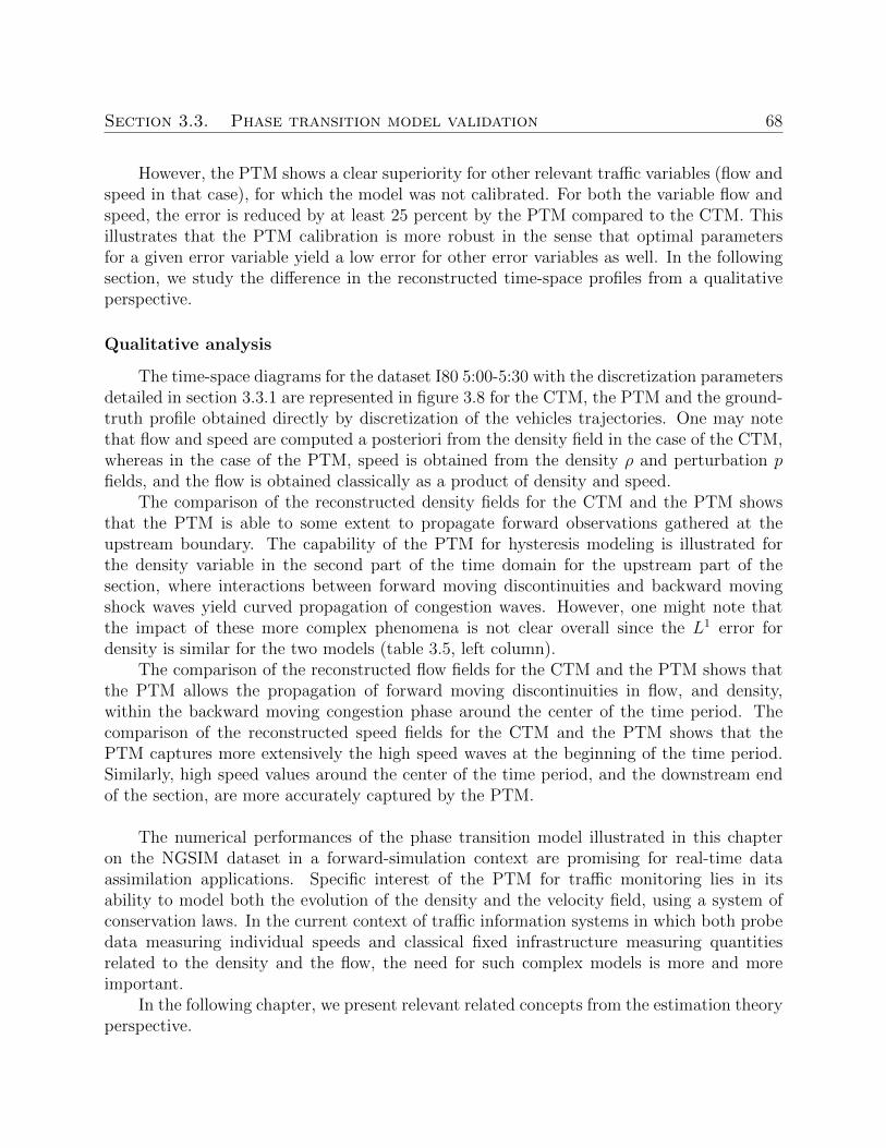
Section 3.3. Phase transition model validation 68
However, the PTM shows a clear superiority for other relevant traffic variables (flow andspeed in that case), for which the model was not calibrated. For both the variable flow andspeed, the error is reduced by at least 25 percent by the PTM compared to the CTM. Thisillustrates that the PTM calibration is more robust in the sense that optimal parametersfor a given error variable yield a low error for other error variables as well. In the followingsection, we study the difference in the reconstructed time-space profiles from a qualitativeperspective.
Qualitative analysis
The time-space diagrams for the dataset I80 5:00-5:30 with the discretization parametersdetailed in section 3.3.1 are represented in figure 3.8 for the CTM, the PTM and the ground-truth profile obtained directly by discretization of the vehicles trajectories. One may notethat flow and speed are computed a posteriori from the density field in the case of the CTM,whereas in the case of the PTM, speed is obtained from the density ρ and perturbation pfields, and the flow is obtained classically as a product of density and speed.
The comparison of the reconstructed density fields for the CTM and the PTM showsthat the PTM is able to some extent to propagate forward observations gathered at theupstream boundary. The capability of the PTM for hysteresis modeling is illustrated forthe density variable in the second part of the time domain for the upstream part of thesection, where interactions between forward moving discontinuities and backward movingshock waves yield curved propagation of congestion waves. However, one might note thatthe impact of these more complex phenomena is not clear overall since the L1 error fordensity is similar for the two models (table 3.5, left column).
The comparison of the reconstructed flow fields for the CTM and the PTM shows thatthe PTM allows the propagation of forward moving discontinuities in flow, and density,within the backward moving congestion phase around the center of the time period. Thecomparison of the reconstructed speed fields for the CTM and the PTM shows that thePTM captures more extensively the high speed waves at the beginning of the time period.Similarly, high speed values around the center of the time period, and the downstream endof the section, are more accurately captured by the PTM.
The numerical performances of the phase transition model illustrated in this chapteron the NGSIM dataset in a forward-simulation context are promising for real-time dataassimilation applications. Specific interest of the PTM for traffic monitoring lies in itsability to model both the evolution of the density and the velocity field, using a system ofconservation laws. In the current context of traffic information systems in which both probedata measuring individual speeds and classical fixed infrastructure measuring quantitiesrelated to the density and the flow, the need for such complex models is more and moreimportant.
In the following chapter, we present relevant related concepts from the estimation theoryperspective.
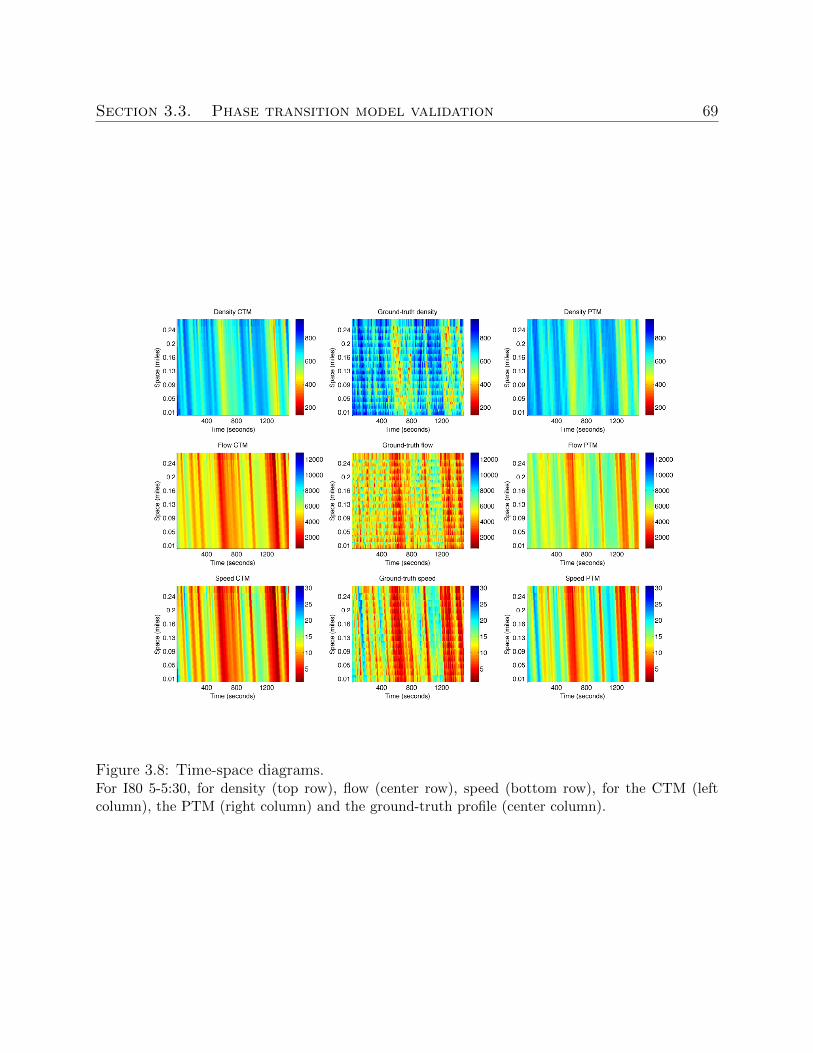
Section 3.3. Phase transition model validation 69
Figure 3.8: Time-space diagrams.For I80 5-5:30, for density (top row), flow (center row), speed (bottom row), for the CTM (leftcolumn), the PTM (right column) and the ground-truth profile (center column).
70
Chapter 4
Advanced estimation methods fordistributed systems
In this chapter, we consider the estimation problem, which consists in the computationof the best estimate of a statistical process, given available measurements and a statisticalor physical underlying model. We present two frameworks in which the estimation problemfor distributed systems can be posed; Bayesian networks articulated around the efficientrepresentation of joint distributions by conditional probabilities, and Kernel methods, whichallow the formulation of the best state-space representation of a given system as a convexoptimization problem.
4.1 Bayesian networks
Most physical principles assumed by classical traffic models can be seen as defininginformation propagation rules. For scalar macroscopic models, the mass conservation prin-ciple yields a partial differential equation (PDE) which can be directly solved by a wavefronttracking method [39], or numerically by the Godunov scheme [103]. Both of these methodsprovide an encoding of the spatio-temporal dependencies of the physical system. Unlike inthe estimation problem, in which the model errors can be corrected via observations, theforecast problem relies heavily on an accurate model as the forecast error grows with thelength of the forecast horizon [131]. Thus, knowing the exact dependency structure of thenetwork is crucial for traffic forecasting applications.
Bayesian networks [125, 128, 184] provide an efficient framework to represent and workwith dependencies in distributed systems, in particular to address fundamental problemssuch as learning and inference. This statistical framework allows us to learn the conditionaldependencies that best fit the data and avoid the need for detailed assumptions regardingthe physical system, which are often unknown or inaccurate. Thus, Bayesian models aremore flexible and capture a variety of traffic phenomena, unlike classical models. Once thedependency structure of the network is identified, it can be used to forecast the evolution of
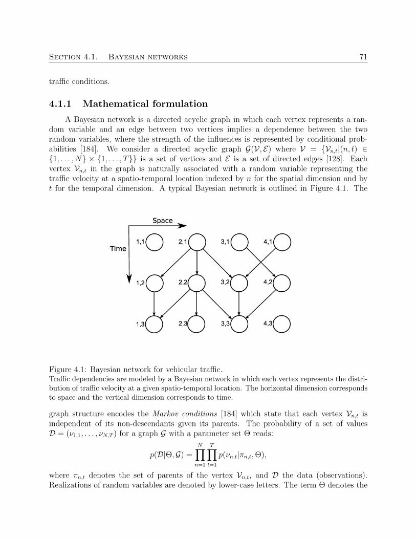
Section 4.1. Bayesian networks 71
traffic conditions.
4.1.1 Mathematical formulation
A Bayesian network is a directed acyclic graph in which each vertex represents a ran-dom variable and an edge between two vertices implies a dependence between the tworandom variables, where the strength of the influences is represented by conditional prob-abilities [184]. We consider a directed acyclic graph G(V , E) where V = Vn,t|(n, t) ∈1, . . . , N × 1, . . . , T is a set of vertices and E is a set of directed edges [128]. Eachvertex Vn,t in the graph is naturally associated with a random variable representing thetraffic velocity at a spatio-temporal location indexed by n for the spatial dimension and byt for the temporal dimension. A typical Bayesian network is outlined in Figure 4.1. The
Figure 4.1: Bayesian network for vehicular traffic.Traffic dependencies are modeled by a Bayesian network in which each vertex represents the distri-bution of traffic velocity at a given spatio-temporal location. The horizontal dimension correspondsto space and the vertical dimension corresponds to time.
graph structure encodes the Markov conditions [184] which state that each vertex Vn,t isindependent of its non-descendants given its parents. The probability of a set of valuesD = (ν1,1, . . . , νN,T ) for a graph G with a parameter set Θ reads:
p(D|Θ,G) =N∏n=1
T∏t=1
p(νn,t|πn,t,Θ),
where πn,t denotes the set of parents of the vertex Vn,t, and D the data (observations).Realizations of random variables are denoted by lower-case letters. The term Θ denotes the
Section 4.1. Bayesian networks 72
parameters of the joint distribution of the graph. The log-likelihood for a dataset D on thegraph G is given by:
l(D; Θ,G) =N∑n=1
T∑t=1
log p(νn,t|πn,t,Θ). (4.1)
In a typical learning framework, in which the conditional distributions are more often avail-able, equation (4.1) conveniently expresses the likelihood of the data in terms of local con-ditional probabilities. In the case in which joint distributions are available, this expressioncan be transformed to:
l(D; Θ,G) =N∑n=1
T∑t=1
log p(νn,t, πn,t|Θ)− log p(πn,t|Θ),
where the first term is assumed to be known as the joint distribution of a vertex and itsparents. The second term can be computed by marginalizing out the vertex Vn,t [128]. Asillustrated in Figure 4.1, Bayesian networks are an efficient tool to represent complex depen-dency relations between random variables. However, Bayesian network theory depends onstrong assumptions regarding the generative distributions being modeled, such as symmetry,decomposition and intersection properties described in [184]. For example, the generativedistribution of G is required to satisfy the decomposition axiom, which states that if ∀ Y ∈ Y ,X is independent of Y , then X is independent of Y (with X, Y being two nodes of the net-work and Y a set of nodes). This property is satisfied by the Gaussian distribution. However,it is not satisfied by most probability distributions (see [184] for an example and [133] forthe general case). This is a strong motivation for the choice of the Gaussian distribution asthe generative distribution for our problem in the following section.
4.1.2 Bayesian network for traffic modeling
In the case of traffic, space and time are discretized into intervals of respective size∆x and ∆t. Each vertex of the Bayesian network has a spatio-temporal index (n, t) ∈1, . . . , N × 1, . . . , T, and thus the Bayesian network has a grid form (Figure 4.1). Inparticular, the discretization grid used for the Godunov scheme could be used for Bayesiannetwork definition. The horizontal dimension represents space and the vertical dimensionrepresents time. Each vertex Vn,t is associated with a probability distribution which rep-resents the traffic velocity at the corresponding spatio-temporal location. A directed edgebetween two vertices implies a dependence between the corresponding velocity distributions.In order to use Bayesian representation of traffic, the following assumptions can be made.
Assumption 4.1. Traffic state evolution can be represented by a Markov process.
In particular the dependency structure learned only depends on the dynamics of thetraffic state. The parameters of the dependency structure are the parameters of the statetransition matrix of a Markov process. This assumption ignores the recurrence of trafficconditions based on the time of day and day of week.
Section 4.1. Bayesian networks 73
Assumption 4.2. Traffic state evolution can be modeled as a linear function of past obser-vations.
For tractability, it is common practice to assume that the traffic state distributions be-long to the Gaussian family. In particular the Gaussian family is closed under the conditionaloperator, and conditional Gaussian distributions have expressions analytical in the parame-ters of the original distributions [83]. Using Gaussian distributions to model spatio-temporaltraffic state dependencies corresponds to the assumption that locally, traffic state evolutioncan be considered to be linear in the observations. According to the triangular model oftraffic [71, 177], this assumption is true within a single traffic phase (free flow or congestion).
Specific traffic properties can be summarized by the following set of constraints C onthe structure of a graphical representation of a traffic model.
C =
∀(νn,t, νn′,t) ∈ V2, (νn,t, νn′,t) /∈ E∀(νn,t, νn′,t′) ∈ V2 s.t. t < t′, (νn′,t′ , νn,t) /∈ E
(4.2)
The first line in equation (4.2) states that there is no direct dependency relationship betweenthe velocity on the highway at two different locations at the same time step. The secondline in equation (4.2) states that the traffic state at a given time period can only impact thetraffic state at a future time period, i.e. information does not propagate backwards in time.
Remark 4.1. Any graph G generated under the structure constraint C expressed by (4.2) isacyclic.
This feature is of crucial importance for the tractability of a structure learning algorithm.
4.1.3 Bayesian structure learning
Problem formulation
Structure learning is a natural problem in Bayesian network theory [125, 128]. Given aset of vertices V and a set of constraints C on the Bayesian network, the structure learningproblem consists of finding an optimal set of edges E and an optimal set of distributionparameters Θ for the application of interest. A standard approach to this problem is themaximization of a score function. In general, for correctness and tractability of use, a scorefunction should satisfy the following properties:
• The decomposability property states that the score can be decomposed in a sum oflocal scores. This allows efficient comparison of structures by local comparisons.
• The asymptotic consistency property states that in the limit of a large number ofsamples, the score function prefers the model with the fewest number of parameters.A more formal definition can be found in [54].
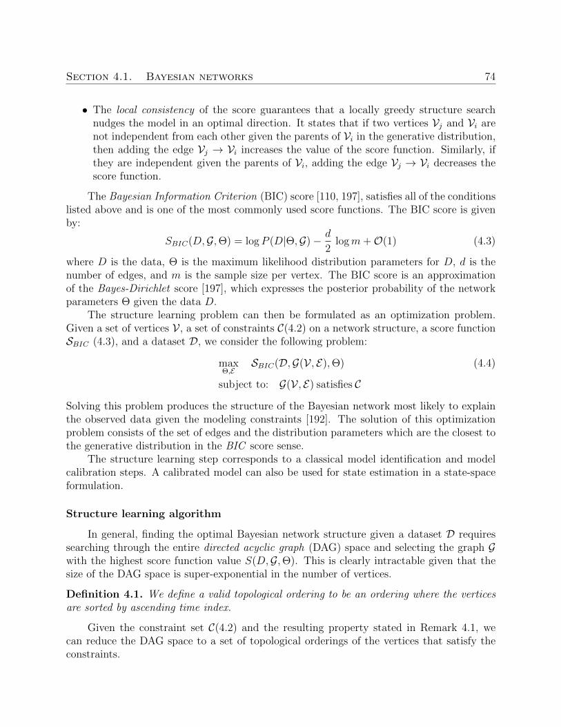
Section 4.1. Bayesian networks 74
• The local consistency of the score guarantees that a locally greedy structure searchnudges the model in an optimal direction. It states that if two vertices Vj and Vi arenot independent from each other given the parents of Vi in the generative distribution,then adding the edge Vj → Vi increases the value of the score function. Similarly, ifthey are independent given the parents of Vi, adding the edge Vj → Vi decreases thescore function.
The Bayesian Information Criterion (BIC) score [110, 197], satisfies all of the conditionslisted above and is one of the most commonly used score functions. The BIC score is givenby:
SBIC(D,G,Θ) = logP (D|Θ,G)− d
2logm+O(1) (4.3)
where D is the data, Θ is the maximum likelihood distribution parameters for D, d is thenumber of edges, and m is the sample size per vertex. The BIC score is an approximationof the Bayes-Dirichlet score [197], which expresses the posterior probability of the networkparameters Θ given the data D.
The structure learning problem can then be formulated as an optimization problem.Given a set of vertices V , a set of constraints C(4.2) on a network structure, a score functionSBIC (4.3), and a dataset D, we consider the following problem:
maxΘ,E
SBIC(D,G(V , E),Θ) (4.4)
subject to: G(V , E) satisfies C
Solving this problem produces the structure of the Bayesian network most likely to explainthe observed data given the modeling constraints [192]. The solution of this optimizationproblem consists of the set of edges and the distribution parameters which are the closest tothe generative distribution in the BIC score sense.
The structure learning step corresponds to a classical model identification and modelcalibration steps. A calibrated model can also be used for state estimation in a state-spaceformulation.
Structure learning algorithm
In general, finding the optimal Bayesian network structure given a dataset D requiressearching through the entire directed acyclic graph (DAG) space and selecting the graph Gwith the highest score function value S(D,G,Θ). This is clearly intractable given that thesize of the DAG space is super-exponential in the number of vertices.
Definition 4.1. We define a valid topological ordering to be an ordering where the verticesare sorted by ascending time index.
Given the constraint set C(4.2) and the resulting property stated in Remark 4.1, wecan reduce the DAG space to a set of topological orderings of the vertices that satisfy theconstraints.
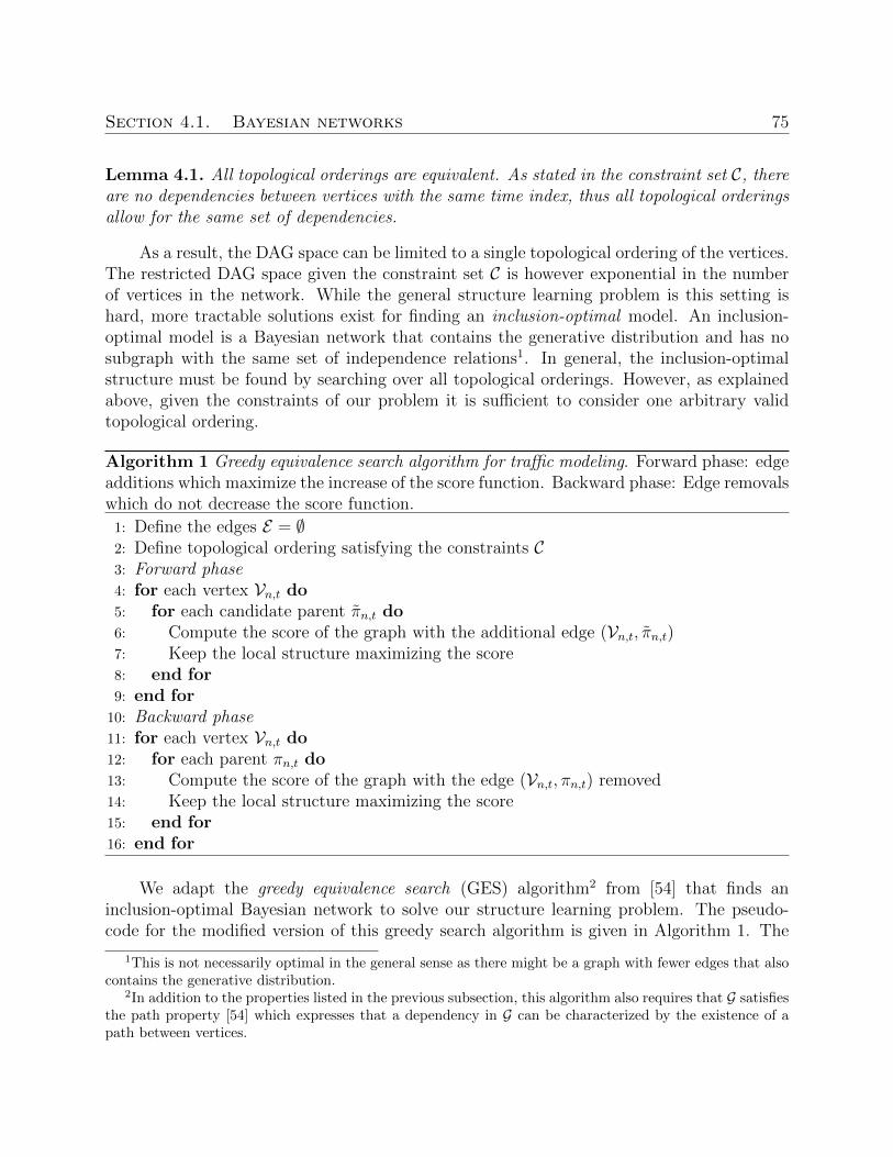
Section 4.1. Bayesian networks 75
Lemma 4.1. All topological orderings are equivalent. As stated in the constraint set C, thereare no dependencies between vertices with the same time index, thus all topological orderingsallow for the same set of dependencies.
As a result, the DAG space can be limited to a single topological ordering of the vertices.The restricted DAG space given the constraint set C is however exponential in the numberof vertices in the network. While the general structure learning problem is this setting ishard, more tractable solutions exist for finding an inclusion-optimal model. An inclusion-optimal model is a Bayesian network that contains the generative distribution and has nosubgraph with the same set of independence relations1. In general, the inclusion-optimalstructure must be found by searching over all topological orderings. However, as explainedabove, given the constraints of our problem it is sufficient to consider one arbitrary validtopological ordering.
Algorithm 1 Greedy equivalence search algorithm for traffic modeling. Forward phase: edgeadditions which maximize the increase of the score function. Backward phase: Edge removalswhich do not decrease the score function.
1: Define the edges E = ∅2: Define topological ordering satisfying the constraints C3: Forward phase4: for each vertex Vn,t do5: for each candidate parent πn,t do6: Compute the score of the graph with the additional edge (Vn,t, πn,t)7: Keep the local structure maximizing the score8: end for9: end for
10: Backward phase11: for each vertex Vn,t do12: for each parent πn,t do13: Compute the score of the graph with the edge (Vn,t, πn,t) removed14: Keep the local structure maximizing the score15: end for16: end for
We adapt the greedy equivalence search (GES) algorithm2 from [54] that finds aninclusion-optimal Bayesian network to solve our structure learning problem. The pseudo-code for the modified version of this greedy search algorithm is given in Algorithm 1. The
1This is not necessarily optimal in the general sense as there might be a graph with fewer edges that alsocontains the generative distribution.
2In addition to the properties listed in the previous subsection, this algorithm also requires that G satisfiesthe path property [54] which expresses that a dependency in G can be characterized by the existence of apath between vertices.
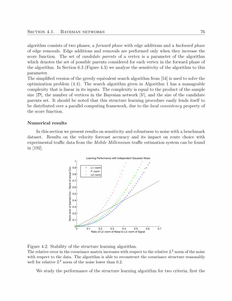
Section 4.1. Bayesian networks 76
algorithm consists of two phases, a forward phase with edge additions and a backward phaseof edge removals. Edge additions and removals are performed only when they increase thescore function. The set of candidate parents of a vertex is a parameter of the algorithmwhich denotes the set of possible parents considered for each vertex in the forward phase ofthe algorithm. In Section 6.3 (Figure 4.3) we analyze the sensitivity of the algorithm to thisparameter.The simplified version of the greedy equivalent search algorithm from [54] is used to solve theoptimization problem (4.4). The search algorithm given in Algorithm 1 has a manageablecomplexity that is linear in its inputs. The complexity is equal to the product of the samplesize |D|, the number of vertices in the Bayesian network |V|, and the size of the candidateparents set. It should be noted that this structure learning procedure easily lends itself tobe distributed over a parallel computing framework, due to the local consistency property ofthe score function.
Numerical results
In this section we present results on sensitivity and robustness to noise with a benchmarkdataset. Results on the velocity forecast accuracy and its impact on route choice withexperimental traffic data from the Mobile Millennium traffic estimation system can be foundin [192].
0 0.1 0.2 0.3 0.4 0.5 0.6 0.70
0.1
0.2
0.3
0.4
0.5
0.6
0.7
0.8
0.9
1Learning Performance with Independent Gaussian Noise
Ratio of L2−norm of Noise to L2−norm of Signal
No
rm e
rro
r o
f le
arn
ed
Co
v.
/ N
orm
of
actu
al C
ov.
L1−norm
F−norm
L2−norm
Figure 4.2: Stability of the structure learning algorithm.The relative error in the covariance matrix increases with respect to the relative L2 norm of the noisewith respect to the data. The algorithm is able to reconstruct the covariance structure reasonablywell for relative L2 norm of the noise lower than 0.2.
We study the performance of the structure learning algorithm for two criteria; first the
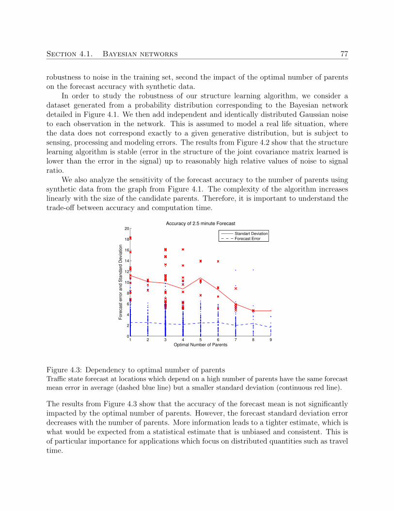
Section 4.1. Bayesian networks 77
robustness to noise in the training set, second the impact of the optimal number of parentson the forecast accuracy with synthetic data.
In order to study the robustness of our structure learning algorithm, we consider adataset generated from a probability distribution corresponding to the Bayesian networkdetailed in Figure 4.1. We then add independent and identically distributed Gaussian noiseto each observation in the network. This is assumed to model a real life situation, wherethe data does not correspond exactly to a given generative distribution, but is subject tosensing, processing and modeling errors. The results from Figure 4.2 show that the structurelearning algorithm is stable (error in the structure of the joint covariance matrix learned islower than the error in the signal) up to reasonably high relative values of noise to signalratio.
We also analyze the sensitivity of the forecast accuracy to the number of parents usingsynthetic data from the graph from Figure 4.1. The complexity of the algorithm increaseslinearly with the size of the candidate parents. Therefore, it is important to understand thetrade-off between accuracy and computation time.
1 2 3 4 5 6 7 8 90
2
4
6
8
10
12
14
16
18
20
Optimal Number of Parents
Fore
cast err
or
and S
tandard
Devia
tion
Accuracy of 2.5 minute Forecast
Standart Deviation
Forecast Error
Figure 4.3: Dependency to optimal number of parentsTraffic state forecast at locations which depend on a high number of parents have the same forecastmean error in average (dashed blue line) but a smaller standard deviation (continuous red line).
The results from Figure 4.3 show that the accuracy of the forecast mean is not significantlyimpacted by the optimal number of parents. However, the forecast standard deviation errordecreases with the number of parents. More information leads to a tighter estimate, which iswhat would be expected from a statistical estimate that is unbiased and consistent. This isof particular importance for applications which focus on distributed quantities such as traveltime.
Section 4.2. Kernel method for state-space identification 78
Bayesian networks are particularly appropriate for the formulation of estimation andforecast problems for distributed systems. However, in the case of unobserved variables, thecomputational cost associated with Bayesian networks can be become significant. In thefollowing section, we present a framework based on convex programming, which allows theidentification of the optimal model parameters in a very efficient manner.
4.2 Kernel method for state-space identification
Kernel regression methods can be considered as an extension of regression techniques,for which the underlying relation between covariates and responses is not pre-defined inadvance.
4.2.1 Regression methods
We consider the following problem of model identification between a set of covariatesxi, e.g. entry times on a road section, and responses yi, e.g. travel-times on the road section.
Given the knowledge of a dataset of sizeN noted S = (xi, yi) ∈ R+ × R+|i = 1, · · · , N,the objective consists of learning a function h : R+ → R+ which given S, would provide anestimate of the travel time y for any x ∈ R+. In the linear case for the L2 norm, thewell-known unconstrained least-squares method reads:
minθ ‖y − xT θ‖22 (4.5)
where y ∈ RN×1 is the vector of realized travel time or output, xT ∈ RN×1 is the vector ofentry time or input. One must note that here x is a row vector and y is a column vector soθ is a scalar. The well-known solution of this problem can be computed as:
θopt = (x xT )† x y (4.6)
where the notation (x xT )† denotes the pseudo-inverse of (x xT ) and the optimal estimate isgiven by y = (x xT )† xT x y. This estimate does not have bias, i.e. the mean of the output yequals the mean of the estimate y.
The regression problem defined in (4.5) is often ill-posed in the sense that the solutiondoes not depend continuously on the data (the case of multiple solutions falls into thatdenomination). Formulation (4.5) could also lead to over-fitting in the case of non-linearregression since there is no penalization for high values of the solution θopt. In order toprevent these two possible flaws, it is a common practice to add to the objective function aquadratic term called Tikhonov regularization [211] which has the form ρ2 |θ|2 in the scalarcase, where the scalar ρ acts as a regulation variable on the penalty. Then the optimalestimate becomes:
y = (x xT + ρ2 I)−1 xT x y. (4.7)
Section 4.2. Kernel method for state-space identification 79
For ρ large enough, the problem is well-posed and over-fitting with respect to θ is pre-vented [88].
4.2.2 Kernel methods
The linear regression method described in section 4.2.1 can be extended to non-linearregression methods through the use of a kernel. One can consider a mapping function φ(·)from the covariates space to a higher-dimensional space, and consider the linear regressionproblem between the mapped covariates φ(xi) and the responses yi. This is the main principleof kernel methods, which consist in using a feature space, in which the dataset is represented,and to consider linear relations between objects in this feature space, and between thesefeatures and the outputs. Given a positive semi-definite matrix K = (kij), we define thekernel function by Kf : X × X → R, where X denotes the covariates space, such thatKf(xi, xj) = kij. This implicitly defines a feature mapping φ(·) between X and a Hilbertspace H by φ(·) : X → H such that 〈φ(xi), φ(xj)〉H = Kf(xi, xj). In the following we noteXmap a matrix representation of the mapping φ(·) (thus the i-th column of Xmap is φ(xi)).When φ(·) has scalar values, Xmap is a row vector.
Remark 4.2. One does not have to define a mapping function φ(·) to define a kernel matrix,but can simply consider a positive semi-definite matrix and use it as a kernel. It is alsopossible to define a kernel matrix from a mapping φ(·) and one of its matrix representationXmap as K = XT
mapXmap.
The inner product in H naturally appears to be given by the Gram matrix K, calledthe kernel. Kernel techniques [68, 194] have several benefits:
• They enable to work with any types of features of the initial data-set, which has apriori no particular structure, in a Hilbert space.
• They guarantee a reasonable computational cost for the algorithm by allowing a com-plexity related to the number of points represented and not the number of featuresused (this is known as the kernel trick and is described in Remark 4.5).
Thus, kernel methods provide several extensions to usual regression methods, and can beeasily written in a machine learning framework.
4.2.3 Kernel learning
Given the knowledge of a training set Str = (xi, yi)|i = 1, · · · , ntr, the kernel learningproblem consists of identifying the best mapping for the elements of the test set, St =xi|i = ntr + 1, · · · , ntr + nt. In order to match the structure of this problem, we define thekernel matrix in block form as:
K =
(Ktr Ktrt
KTtrt Kt
)(4.8)
Section 4.2. Kernel method for state-space identification 80
where kij = 〈φ(xi), φ(xj)〉H for i, j = 1, · · · , ntr, ntr + 1...ntr + nt. Kt denotes the innerproducts between the elements of the test set. The Gram matrix Ktr is the result of anoptimization problem over the training set, and we learn the cross-term Ktrt, which expressesthe inner-product in the feature space between the elements of the test-set and the elementsof the training set.
Convex formulation of the kernel learning problem
In this section we formulate the kernel learning problem as a convex problem. Express-ing the linear least-squares (4.5) for the mapped input Xmap with the regularization termdescribed in section 4.2.1 yields:
p∗ = minθ ‖y −XTmap θ‖2
2 + ρ2 ‖θ‖22 (4.9)
where we note p∗ the optimal value of this problem. Using the change of variable z =XT
map θ − y yields the equivalent formulation:
p∗ = minθ,z ‖z‖22 + ρ2 ‖θ‖2
2 (4.10)
subject to z = y −XTmap θ (4.11)
The Lagrangian dual of this problem reads:
d∗ = maxα
(−2αT y − αT
(I +
XTmapXmap
ρ2
)α
). (4.12)
In this equation, we see the expression of the kernel matrix:
K = XTmapXmap. (4.13)
If we denote Kρ = I +XT
mapXmap
ρ2the regularized kernel, the dual optimal point and dual
optimal value of problem (4.12) can be expressed as:
α∗ = K−1ρ y and d∗ = yT K−1
ρ y. (4.14)
Remark 4.3. Since the primal (4.10)-(4.11) and dual (4.12) are convex and strictly feasible,strong duality holds and primal optimal value p∗ and dual optimal value d∗ are equal. Wenote that expression (4.12) shows that the dual optimal value is a maximum over a set oflinear functions of Kρ, so the optimal value is a convex function of the regularized kernelmatrix Kρ. Since the choice of the kernel is crucial for the optimal value, it is interesting tominimize the optimal value d∗ with respect to the kernel.
Remark 4.4. Optimizing the kernel matrix physically means looking for the best mappingfunction φ(·) such that there is a linear relation between the features of the inputs φ(xi) and
Section 4.2. Kernel method for state-space identification 81
the outputs yi. If one takes φ(·) as the identity mapping, then the optimal value of (4.12)becomes:
yT K−1ρ y = yT
(I +
xT x
ρ2
)−1
y (4.15)
which may not be optimal for non-linear systems.
Remark 4.5. One must note that the kernel matrix (4.13) is a square matrix which has thedimension of xT x, and thus its size does not depend on the number of features representedin Xmap but only on the number of covariates xi. The dimension of the image space of φ(·),which is the dimension of the feature space, does not appear in the kernel matrix. This isthe kernel trick mentioned in section 4.2.2.
Cross-validation
The optimal value of (4.9) as expressed in (4.14) depends on the kernel matrix (4.13)and on the regularization parameter ρ. The parameter ρ is tuned through a re-samplingprocedure [86], the k-fold cross-validation (here k does not denote the kernel matrix but thenumber of folds used in the cross-validation method). This technique consists in dividing thedataset into k parts of approximately equal size, and using a subset for training while theremainder is used for testing [215]. For instance if the different parts are Pi|i = 1, · · · , kthen given n ∈ 1, · · · , k one would use Pn as a training set and
⋃i=1,··· ,k, i6=n Pi as a test set.
This is useful to make extensive use of the dataset while avoiding bias on the training set.Here we use this method on the training set to pick the optimal value of the regularizationparameter ρ and on the whole set to have a meaningful estimation error.
Kernel regression
As stated in Remark 4.3, the optimal value of the regularized regression problem (4.9) isa convex function of the regularized kernel matrix Kρ and can be optimized over the kernel.The kernel optimization problem, which consists in minimizing the value d∗ defined in (4.14)with respect to the regularized kernel Kρ reads:
minKρ yT K−1ρ y (4.16)
subject to Kρ ≥ 0 (4.17)
where the constraint on the kernel matrix enforces that the regularized kernel Kρ must bea Gram matrix. This problem is convex according to Remark 4.3. In order to prevent over-fitting with respect to Kρ, we follow [142] and constrain Kρ to be a convex combination of
Section 4.2. Kernel method for state-space identification 82
given kernels, i.e. we define a set of kernels K1, · · · , Kk and consider the problem:
minλ yT K−1ρ y (4.18)
subject to λi ≥ 0k∑i=1
λi = 1 (4.19)
Kρ =k∑i=1
λiKi. (4.20)
In a learning setting, the optimization problem (4.18) is defined only on the training set butthe expression of the kernel matrix as a linear combination of known kernels must be satisfied
on the entire set. Using the notation introduced in (4.8) we write Kρ =
(Ktr Ktrt
KTtrt Kt
)and
under this form the problem reads:
minλ yT K−1tr y (4.21)
subject to λi ≥ 0k∑i=1
λi = 1 (4.22)
Kρ =k∑i=1
λiKi (4.23)
which can be written in a semi-definite program form using an epigraphical property andthe Schur complement:
minλ,t t (4.24)
subject to λi ≥ 0k∑i=1
λi = 1 (4.25)
Kρ =k∑i=1
λiKi and
(t yT
y I + Ktr
ρ2
)≥ 0. (4.26)
The solution of this optimization problem is the parameter λ∗ giving the optimal convexcombination of the set of kernels K1 · · ·Kk which minimizes d∗ from (4.14).
Rank-one kernel optimization
The kernel optimization problem in the form of (4.24)-(4.25)-(4.26) is not tractable andcannot be efficiently solved by standard optimization software. A rank-one decomposition ofkernels can be used in order to find an equivalent formulation in a linear program form. Thisis done through the introduction of several intermediate problems. Assuming we can writethe regularized kernel as a convex combination of dyads: Kρ =
∑pi=1 νi li l
Ti where li are row
Section 4.2. Kernel method for state-space identification 83
vectors and νi are positive scalars such that∑p
i=1 νi = 1. Since by definition Kρ = I + Kρ2
,the decomposition of Kρ into a sum of dyads is possible whenever the kernel K itself can bewritten as a sum of dyads. In practice, the kernel is a positive semi-definite matrix, so it canbe diagonalized in an orthonormal basis and this property is satisfied. Thus, we can writean equivalent formulation of problem (4.18)-(4.19)-(4.20) as:
Ψ = minν yT K−1ρ (ν) y (4.27)
subject to νi ≥ 0
p∑i=1
νi = 1 (4.28)
Kρ =
p∑i=1
νi li lTi (4.29)
where the vectors li are the eigenvectors of the matrices Kj from equation (4.20). Introducingthe change of variable κ = K−1
ρ (ν) and doing some computations enables one to rewriteproblem (4.27)-(4.28)-(4.29) as:
Ψ = maxκ
(2 yT κ− max
1≤i≤p(lTi κ)2
)(4.30)
and the optimal κ is related to the optimal ν by the following relation
κ∗ = K−1ρ (ν∗). (4.31)
One can note that solving problem (4.30) for the vector variable κ is the same as solving theproblem:
Ψ = maxγ,β
(2 yT γ β − max
1≤i≤p(lTi γ β)2
)(4.32)
for the variables γ and β. This is simply obtained by writing κ = γ β in problem (4.30),with γ scalar and β vector. The optimal point (γ∗, β∗) of problem (4.32) satisfies:
Ψ1/2 β∗ = γ∗ β∗ = κ∗. (4.33)
If we minimize over γ in (4.32) we obtain the following optimization problem:
Ψ1/2 = maxβ yT β (4.34)
subject to |lTi β| ≤ 1 i = 1, ..., p. (4.35)
The Lagrangian of this problem can be written as:
L(β, u) = yT β +
p∑i=1
(|ui| − ui
(lTi β
))(4.36)
Section 4.2. Kernel method for state-space identification 84
and taking the Lagrangian dual of problem (4.34)-(4.35) yields:
Ψ1/2 = minu ‖u‖1 (4.37)
subject to y =
p∑i=1
ui li (4.38)
using the strict feasibility of the primal and convexity of the primal and the dual. Prob-lem (4.38) is a linear program. The optimal ν∗ can be retrieved from the optimal u∗ fromthe relation:
ν∗i =|ui|∗
Ψ1/2. (4.39)
Indeed one can check that with this value of the vector ν equations (4.31)-(4.33) yieldsΨ1/2Kρ(ν
∗) β∗ = y and on the other hand we can write Ψ1/2Kρ(ν∗) β∗ =
∑pi=1 |u∗i | (lTi β) li
which is equal to∑p
i=1 ui li using the optimality condition in the Lagrangian (4.36). Thisproves that if u∗ is optimal for (4.37)-(4.38) then ν∗ given by (4.39) is optimal for (4.27)-(4.28)-(4.29) and vice-versa.
Kernel learning and kernel regression methods have been mostly applied to static ma-chine learning problems. A corresponding theory for dynamical and distributed systems isstill the topic of active research.
In the following chapter, we present how a control-theoretical formulation of Bayesiannetworks, namely nonlinear filtering techniques, can be applied to scalar hyperbolic conser-vation laws, and the extent to which discontinuity and non-differentiability of the solutionto the partial differential equations impact the optimality of the resulting estimates.
85
Chapter 5
Sequential data assimilation for scalarmacroscopic traffic flow models
In this chapter we consider the problem of sequential data assimilation for the nonlinearpartial differential equations traffic models presented in the previous chapters. As mentionedbefore, the estimation for nonlinear systems requires the use of suboptimal techniques forwhich there is no analytical or numerical access to the optimum. The focus of this chapter ison the analysis of the impact of the specific properties of the solutions to partial differentialequations based traffic models, onto the optimality of the estimates provided by classicaladvanced filtering techniques.
The estimation problem for nonlinear systems has been heavily studied in particularwithin the meteorology community, with subsequent development of sophisticated data as-similation techniques [36, 152], which fall into two major categories: variational methods andoptimal interpolation methods. Variational methods [152] consist of finding the solution ofa model (with or without stochastic forcing) which minimizes a certain distance to observa-tions. Estimates provided by optimal interpolation methods are not in general solutions toa model, but minimize a weighted distance to the model solution and to the observations.In meteorology, a common example of a variational method is the 3D-Var algorithm [65] forthe static problem and 4D-Var algorithm in the time-varying case [66].
The theory of inverse problems [131] is concerned with the estimation of model parame-ters. A specific type of inverse methods consists in iteratively updating the estimates as databecomes available [91], instead of solving an inverse problem once using all measurements inbatch. These so-called sequential estimation algorithms, particularly appropriate for on-lineestimation, often rely on Bayes rule and a computationally explicit optimality criterion (e.g.Gauss-Markov theorem for minimum mean squared error estimation). In the case of additivenoise, one of the most well-known sequential estimation algorithms is the seminal Kalmanfilter [132].
Section 5.1. Data assimilation 86
5.1 Data assimilation
5.1.1 Application to transportation networks
In the transportation field, applications of sequential state estimation date back to the1970’s and the work of Gazis [100, 208], who independently used the Kalman Filter (KF)and the Extended Kalman Filter (EKF) to estimate traffic density in the Lincoln tunnel,New-York, for the purpose of traffic control. More recent work from Papageorgiou [221, 222]involves the application of the EKF to a non-scalar traffic model [182]. The EKF has alsobeen applied [196] to the LWR equation with a Smulders [201] flux function.
The Mixture Kalman Filter (MKF) [51] is an extension of the KF to conditionally lineardynamical systems. The MKF has been applied in the transportation community [114, 206,209] to the cell-transmission model (CTM) [71, 72], which exhibits piecewise linear dynamics,conditioned on the phases of traffic (free-flow, congestion) upstream and downstream.
In the recent years, sequential Monte Carlo methods, or Particle Filters (PF), and so-called ensemble methods such as the EnKF have been applied to traffic estimation [171, 227,228]. Ensemble methods [93] consist of representing the first moment of the state estimatedistribution by a set of samples and using a linear measurement update, whereas particlemethods [105] consist in propagating a sample representation of the full distribution of theestimate and using a nonlinear measurement update.
Another notable filter is the Unscented Kalman Filter (UKF) [129] which introducesan unscented transformation providing an exact representation of the first two momentsof a distribution by a set of deterministically determined samples (see [170] for a trafficapplication).
A variety of traffic models and filters have been shown to perform well for practicalapplications. However, the problem of the structural limits of data assimilation algorithmsfor traffic estimation has not received much attention. It is well-known that, in practice,high accuracy can be achieved with sufficiently accurate measurements in sufficiently largevolumes. But with massive datasets coming from increasingly diverse sources, traceabilityand high quality of traffic data are not necessarily guaranteed. Being able to identify theestimation errors inherent to the structure of traffic phenomena is required for the designof more robust, transparent data assimilation algorithms, and scalable, appropriate datacollection methodologies.
In this chapter, we analyze the structural properties of one of the most classical macro-scopic traffic flow models, the Lighthill-Whitham-Richards (LWR) partial differential equa-tion (PDE) [159, 189], in the context of estimation. We present the difficulties resultingfrom these properties, which create significant challenges for the design of an optimal filter-ing algorithm for this model.
Section 5.1. Data assimilation 87
5.1.2 Optimal filtering for LWR PDE
Structural properties of the LWR PDE and its discretized forms impact the optimalityof estimates produced by classical sequential estimation techniques. The focus of this chap-ter is on the analysis and quantification of the lack of estimate optimality resulting from thefollowing properties of the LWR PDE, and its numerical discretization using the Godunovscheme.
Nonlinearity of the fundamental diagram
One of the main properties of the LWR PDE is the nonlinearity of its flux function (fun-damental diagram), which allows the modeling of traffic phases of different nature: free-flowand congestion. Nonlinearities of the model are the cause of the appearance of discontinuitiesin the solution of the partial differential equation. Consequently, the distribution of the un-certainty on the true state is a mixture distributions at shock waves even for unimodal noisedistributions on the initial condition. In this chapter, we analytically show the emergence ofmixture distributions in the solution of the PDE and numerically illustrate their importanceon benchmark tests.
The mixture nature of the distribution of the uncertainty on the true state resultingfrom initial condition uncertainty propagating through an uncertain model raises the ques-tion of the relevance of minimal variance estimate for traffic applications. The estimate meanproduced by classical filters may indeed correspond to a state with zero true probability, andthe estimate covariance may exhibit large values corresponding to a variability due to thecoexistence of different modes in the distribution of the uncertainty on the true state, eachwith significantly smaller covariance.
Non-differentiability of the discretized model
The most common numerical scheme used to compute the solution of the LWR PDEis the Godunov scheme [103], a finite volume scheme which consists of iteratively solvingRiemann problems [89] between neighboring discretization cells and averaging their solutionat each time-step on each spatial cell, as described in Chapter 1. In this chapter we provethat this scheme is non-differentiable and we derive the expression of its non-differentiabilitydomain.
The lack of differentiability of the Godunov scheme, a common discretization of theLWR PDE, is relevant for data assimilation algorithms whose optimality guarantees arebased on Taylor series analysis, which assumes exact computation of the derivative up toa certain order. This is the case in particular for the EKF, which considers propagationof the estimate covariance using the tangent (linearized) model. Numerical results quantifyestimate errors induced by this property of the discretized model. The result also affectsknown order of accuracy of the estimate moments of the UKF, since in this case the Taylorseries does not exist up to the required order.
Section 5.2. Nonlinear estimation 88
This chapter can thus be viewed as a theoretical and numerical study of the implicationsof the structural properties of the Godunov scheme and CTM on filtering algorithms. Itsheds some new light on the proper use of these schemes for traffic estimation purposes, andprovides conclusions which are illustrated by detailed numerical studies.
While the results presented here are derived for the Godunov scheme, because histori-cally is was one of the first numerical schemes proposed to solve scalar hyperbolic conservationlaws (and the LWR PDE in particular), other proposed schemes such as the CTM exhibitthe same features as the Godunov scheme, and thus our analysis applies to them as well.
The remainder of the chapter is organized as follows. Section 5.2 introduces the generaltheory of sequential data assimilation and optimal filtering. Section 5.3 focuses on theRiemann problem which is the keystone of numerical solutions of continuous and discretescalar conservation models and the focus of our subsequent analysis. Section 5.4 and 5.5point at the structural properties of macroscopic traffic models derived from the LWR PDE,in particular model nonlinearity in Section 5.4 and model non-differentiability in Section 5.5.
5.2 Nonlinear estimation
5.2.1 Deterministic filters
In this section we present the EKF and the UKF for nonlinear systems. The EKFforecast step is based on model linearization. The UKF consists in representing exactly thefirst two moments of the prior distribution by a set of deterministic samples. In particular,no sampling term is required for the application of these algorithms.
Extended Kalman filter
The EKF is an extension of the KF for nonlinear state-space models. The EKF consistsin using a Taylor series truncation of the model at the current state to propagate the statestatistics. We present the case of a nonlinear state model combined with a linear observationmodel, although nonlinear observation equation can also be considered through a similarlinearization of the observation operator at the analysis step. The forecast mean is givenby a zero-th order truncation of the model, whereas the forecast covariance is given by afirst order truncation of the model. If we note At+1 the linearization of the nonlinear modeldynamics A(p, t) at the state estimate p, the forecast and analysis steps for the EKF read:
Forecast:
xt+1|t = A(xt|t, t)
Σt+1|t = At+1 Σt|tATt+1 +Wt+1
(5.1)
Analysis:
xt+1|t+1 = xt+1|t +Kt+1
(yt+1 − Ct+1 xt+1|t
)Σt+1|t+1 = Σt+1|t −Kt+1Ct+1 Σt+1|t
where Kt+1 = Σt+1|tCTt+1
(Ct+1 Σt+1|tC
Tt+1 + Vt+1
)−1
(5.2)
Section 5.2. Nonlinear estimation 89
where the only difference with the Kalman filter resides in the propagation of the state meanat the forecast step, using the nonlinear state model. Different sources of sub-optimalityarise in the derivation of the EKF:
1. Accuracy of the Taylor truncation:
a The model approximation used at the forecast step (5.1) for the covariance propa-gation requires that the model Jacobian be accurately computed.
b The mean given by the EKF is a second order Taylor series approximation of theMMSE, whereas the covariance is a fourth order approximation of the MMSE errorcovariance.
2. Closure assumption: it is assumed that there is no significant interaction betweenhigher order statistics and the first two moments of the state estimate.
Cases in which the closure assumption breaks, due to the importance of higher order termsin the model Taylor series have been documented, with illustrations of estimates biased andinconsistent [129], and with diverging error statistics [90]. Cases in which this assumptionbreaks, due to the importance of higher-order statistics can be found in [172, 173] in the caseof bimodal distributions.
Remark 5.1. An approximation made in the EKF equations lies in the propagation of thestate covariance Σt+1|t. This covariance is then used at the analysis step (5.2) at whichobservations are combined with the model forecast. The study of the resulting error structureof the state covariance after propagation in the context of traffic is to the best of our knowledgean open problem, and is a focus of the research presented in this chapter.
Unscented Kalman filter
The UKF [129] is built on the unscented transformation, which consists in representinga distribution with mean µ and variance Σ by a set of weighted samples, or sigma points,chosen deterministically such that the weighted sample mean is µ and the weighted samplecovariance is Σ [130]. For for a state-space of dimension n, the 2n+1 sigma points producedby the unscented transformation are defined as
x0 = µ
xk = µ+ ((n+ k) Σ)12k k = 1, . . . , n
xk+n = µ− ((n+ k) Σ)12k k = 1, . . . , n
(5.3)
where ((n+ k) Σ)1/2k denotes the kth column of the square root of (n+k) Σ. The correspond-
ing weights wk are parameterized by κ, which controls the spread of the sigma points:w0 = κ
κ+n
wk = 12(κ+n)
k = 1, . . . , n
wk+n = 12(κ+n)
k = 1, . . . , n.
(5.4)
Section 5.2. Nonlinear estimation 90
Choosing the samples according to (5.3) and the weights according to (5.4) yields that theweighted sample mean and weighted sample covariance are equal to the distribution meanand covariance for any choice of κ. The forecast and analysis step of the UKF can be writtenas follows:
Forecast:
Propagate sigma-points
xkt+1|t = A(xkt|t, t) k = 1, . . . , 2n+ 1
Compute forecast mean and covariance
xt+1|t =∑2n+1
k=0 wk xkt+1|t
Σt+1|t =∑2n+1
k=0 wk
(xkt+1|t − xt+1|t
) (xkt+1|t − xt+1|t
)T(5.5)
Analysis:
Compute sigma-points observations
zkt+1|t = Ct+1 xkt+1|t k = 1, . . . , 2n+ 1
Compute observation mean and covariance
zt+1|t =∑2n+1
k=0 wk zkt+1|t
Zt+1|t =∑2n+1
k=0 wk
(zkt+1|t − zt+1|t
) (zkt+1|t − zt+1|t
)TCompute covariance between forecast and observation
Yt+1|t =∑2n+1
k=0 wk
(xkt+1|t − xt+1|t
) (zkt+1|t − zt+1|t
)TCompute posterior mean and covariance
xt+1|t+1 = xt+1|t +Kt+1
(yt+1 − zt+1|t
)Σt+1|t+1 = Σt+1|t −Kt+1 Zt+1|tK
Tt+1
where Kt+1 = Yt+1|t Z−1t+1|t
(5.6)
where the unscented transformation is first used to compute the sigma points for the currentestimates, which are then propagated through the model and whose mean and covariance iscomputed (5.5). At the analysis step, the forecast observation associated with each sigmapoint through the (potentially) nonlinear observation model Ct+1, is computed as zkt+1|t,which allows the computation of the observation mean zt+1|t, observation covariance Zt+1|t,and the covariance between forecast state and observation as Yt+1|t. The analysis mean andcovariance are then computed exactly using Kalman equations (5.6).
Different sources of sub-optimality arise in the UKF:
1. Limited number of samples: the mean and the covariance propagated by the UKFare fourth order approximations of the MMSE and MMSE error covariance.
2. Closure assumption: it is assumed that there is no significant interaction betweenhigher order statistics and the first two moments of the state estimate.
The UKF has been applied to traffic estimation [170] and was compared with the EKFfor the Papageorgiou model (1.10). The two filters were empirically shown to have simi-lar performances for joint state and parameter estimation [111] for this model (1.10). The
Section 5.2. Nonlinear estimation 91
results of this comparison are completed by the analysis presented in Section 5.4 and Sec-tion 5.5, in which we study the state distribution features due to model nonlinearities andnon-differentiability analytically and numerically in the case of the LWR model, and in whichwe show how they affect the EKF and the UKF. In particular we analyze the true distri-bution structure at shock waves of the LWR model, in the continuous and discrete domain.The Papageorgiou model is defined in the discrete domain, and exhibits an anticipation termwhich reduces the sharpness and amplitude of spatial variations. Consequently, the impactof the existence of shock waves on the performance of the filters is stronger in the case ofthe LWR model in the continuous domain.
5.2.2 Stochastic filters
A wide variety of filters extend the Kalman filter for nonlinear state models by represent-ing the state by a set of random samples (particles, ensemble members). The rules for samplepropagation, update, and for resampling, are of different types. The need for pseudo-randomgenerator at every step of these algorithms justifies the appellation stochastic filters.
Ensemble Kalman filter
The EnKF [92, 93] consists in representing the state statistics by a set of ensemblemembers which are evolved in time and whose mean is an estimator of the true state. Thestate error covariance is represented by the ensemble covariance. Formally, with N ensemblemembers, the EnKF equations read:
Forecast:
xkt+1|t = A(xkt|t, t) + wkt+1 k = 1, . . . , N
xt+1|t = 1N
∑Nk=1 x
kt+1|t
Σt+1|t = 1N−1
∑Nk=1
(xkt+1|t − xt+1|t
)(xkt+1|t − xt+1|t
)T (5.7)
Analysis:
xkt+1|t+1 = xkt+1|t +Kt+1
(yt+1 + vkt+1 − Ct+1 xt+1|t − vt+1
)k = 1, . . . , N
Σt+1|t+1 = Σt+1|t −Kt+1Ct+1 Σt+1|t
where Kt+1 = Σt+1|tCTt+1
(Ct+1 Σt+1|tC
Tt+1 + Vt+1
)−1
(5.8)
where we noted v the mean of v. In the limit of large number of samples, the EnKF convergestoward the KF for linear systems. Due to the independent ensemble forecasts (5.7), it isembarrassingly parallel and particularly appropriate for efficient distributed computations.At the analysis step (5.8), the modeled observation noise is explicitly added to the measuredobservation, to capture the full observation noise in the analysis equation [42]. In the contextof traffic estimation, the EnKF has been applied to the Bay Area highway networks witha traffic model equivalent to the LWR PDE, formulated in the velocity variable [227]. Theprincipal source of sub-optimality arising in the EnKF is sampling error:
Section 5.2. Nonlinear estimation 92
1. Sampling error: the use of a finite number of ensemble members introduces a sam-pling error in the estimate distribution.
Remark 5.2. The covariance given by the EnKF is the state error covariance and not thestate covariance. In the KF, the state mean and state error covariance are propagated ana-lytically. The state error covariance coincides with the state covariance. On the other hand,the EnKF analytically propagates ensemble members whose mean is an unbiased estimator ofthe state mean, and covariance coincides by definition of the update equations with the stateerror covariance, but not with the state covariance, except in the limit of an infinite numberof ensemble members.
Extensions of the EnKF giving access to higher order moments of the state distribution havealso been considered [10] by integrating a modified analysis step.
Particle filter
The PF, also known as bootstrap filter, or sequential Monte Carlo method [11, 105, 163]can be traced back to the seminal articles of Metropolis and Ulam [169], later generalized byHastings [109]. These methods represent the full statistics of the state by a set of sampleswhich are propagated through the state model. When observations are received, sampleweights are scaled by the relative likelihood of the new observation, and the updated repre-sentation of the probability distribution is re-sampled. Formally, the PF steps in the case ofN particles are as follows:
Forecast: xkt+1|t = A(xkt|t, t) + wkt+1 k = 1, . . . , N
Analysis:
Re-weighting:
αkt+1 = αktp(yt+1|xkt+1|t)∑N
k=1 αkt p(yt+1|xkt+1|t)
k = 1, . . . , N
Re-sampling:
Generate N samples xkt+1|t+1 from the distribution defined by
P (X = xkt+1|t+1) = αkt+1, k = 1, . . . , N
The PF has been applied to the case of transportation systems [171] on the stochastic modeldescribed in [34]. The particle filter is the only filtering method able to capture the completestate distribution, in the limit of infinite number of samples, without restrictive assumptionon the dynamics or on the statistics. Well-known weaknesses of the PF relate to the problemof sample degeneracy for high dimensional [202] systems. The use of an appropriate proposaldistribution at the re-weighting step is key to reducing the sample weight variance given thesystem history, but more sophisticated importance sampling or rejection sampling techniquesare often considered [11, 218]. The sources of sub-optimality in the PF relate to:
1. Sampling error: the use of a finite number of particles introduces a sampling errorin the estimate distribution.
Section 5.3. Discontinuities and uncertainty 93
The implicit particle filter is a notable extension [55] of the PF which allows a-priori thedefinition of the desired weights of the particles after analysis and thus alleviation of theproblem of sample degeneracy in the case of the exponential family. Another research trackhas explored the use of the EKF, EnKF or UKF to compute the proposal distribution in theparticle filter [218].
Sustained improvements of the filters presented above have been in large part driven byspecific improvements for systems exhibiting strong nonlinearity or non-normality, identifiedas the causes of inaccurate estimates and forecast. In the following section, we present theseminal macroscopic traffic models which have been considered for real-time data assimilationon transportation networks. The subsequent sections will then focus on the analysis of theperformance of the respective filtering schemes on the models.
5.3 Discontinuities and uncertainty
At the macroscopic level, traffic flow exhibits nonlinearities which can be modeledusing nonlinear conservation laws such as the LWR PDE. Nonlinearities are the cause fordiscontinuities which may arise in finite time in the solution to the Cauchy problem associatedwith the PDE even with smooth initial and boundary data. According to the definition of thesolution to the Riemann problem (5.10), shock waves persist when, at a spatial discontinuity,the upstream density is lower than the downstream density. Thus they cannot be neglectedby any traffic application. Physically, these discontinuities model the existence of queues,which are one of the main focus of traffic flow research.
5.3.1 Estimation and control
Queues extremities are phenomena with very limited spatial extent, which characterizethe interface between significantly different phases of traffic flow. This property makes themrelatively hard to directly measure and monitor using classical fixed sensing infrastructure.This is especially true when the upstream end of the queue is stationary, and can only bedirectly measured if it lies on a fixed sensor or by probe vehicles reporting measurementsexactly at the corresponding location.
Large traffic variations occurring on a short spatial extent, typical of queues extremities,make them particularly hazardous, and being able to alert drivers of sudden changes in speedis one of the focal points of traffic safety applications [119].
For control applications, accurately locating the location and propagation speed ofqueues is critical. Their location typically impacts ramp metering algorithms directly, sincethey are often designed around the values of the upstream and downstream flow at the up-stream end of the queue. In the absence of sensors, the algorithm depends on the estimatedflows upstream and downstream of the ramp.
Furthermore, accurate estimation of the propagation speed of queues is one of the mostessential components of traffic forecast and dynamic travel-time estimation. Estimating
Section 5.3. Discontinuities and uncertainty 94
their propagation speed requires the estimation of the left and right density at the queueextremities, as well as accurate knowledge of the fundamental diagram.
In the context of model-based estimation, the influence of model nonlinearity and non-differentiability on the quality of the estimates for traffic phenomena has not received muchattention in the traffic community with a few notable exceptions [111, 207] (see [33] for arelated problem for atmospheric models, and [50] for a study of non-differentiability in ageneral context). In the following section, we consider the Riemann problem, which is abenchmark problem for studying the solution to the LWR PDE, and the evolution of shockwaves. We then consider in Section 5.3.3 the Riemann problem with stochastic datum,which is used in the following sections as a framework for the study of the propagation ofdiscontinuities in presence of uncertainties.
5.3.2 Riemann problem
The Riemann problem is a Cauchy problem with a self-similar initial condition, of theform:
ρ(t = 0, x) =
ρl if x < 0
ρr if x > 0(5.9)
The solution to the Riemann problem is the solution to the Cauchy problem associatedwith the PDE with initial condition the Riemann datum (5.9). The Riemann problem isa key building block for proofs of existence of solutions to the Cauchy problem for generalinitial conditions in the space of bounded variations (BV), via Helly’s theorem [39]. It is alsocritical to the design of numerical schemes such as the wavefront tracking method [39] andthe Godunov scheme, which proceeds by iteratively solving the Riemann problem betweendiscretization cells, before averaging its solution on each cell (see equations (1.7) and (1.8)).
For a flux function Q(·) with constant concavity sign, the unique entropy solution tothe Riemann problem is defined for (t, x) ∈ R+\0 × R as follows
1. If Q′(ρl) > Q′(ρr) the solution is a shock wave
ρR
(xt, ρl, ρr
)=
ρl for x
t< σ
ρr for xt> σ
(5.10)
where the location of the discontinuity is x = σt, with σ given by the Rankine-Hugoniotrelation:
σ =Q(ρl)−Q(ρr)
ρl − ρr(5.11)
which expresses the conservation of ρ at the discontinuity.
2. If Q′(ρl) < Q′(ρr) the solution is a rarefaction wave
ρR
(xt, ρl, ρr
)=
ρl for x
t≤ Q′(ρl)
(Q′)−1(xt) for x
t∈ (Q′(ρl), Q
′(ρr))
ρr for xt≥ Q′(ρr)
Section 5.3. Discontinuities and uncertainty 95
The interested reader is referred to Evans [89] and Leveque [156] for more details, andPiccoli [97] in the context of traffic. Shock waves and rarefactions waves respectively modelthe upstream and downstream ends of a queue. One may note that depending on the flowdifference at the discontinuity, the propagation speed may be positive or negative.
Remark 5.3. This brief description of the Riemann problem for the scalar conservationlaw is also of interest for continuous non-scalar traffic models in which discontinuities arise(see [31, 231]).
For estimation purposes, it is appropriate to consider uncertain Riemann datum, whichrequires the definition of the Riemann problem with stochastic datum.
5.3.3 Riemann problem with stochastic datum
We consider a Riemann problem for a scalar conservation law with concave flux, withstochastic datum [69] defined by:
ρ(t = 0, x) =
%l if x < 0
%r if x > 0(5.12)
where %l, %r are random variables. We further note ς the random variable defining the re-sulting shock speed, whose distribution is given by the distribution of the Rankine-Hugoniotspeed (5.11) for the realizations of the stochastic datum (%l, %r). We focus our analysis onthe case in which each realization of the solution to the Riemann problem with stochasticdatum is a shock wave. In the following proposition, we derive the analytical expression ofthe random field solution of the Riemann problem with stochastic datum in this case.
Proposition 5.1. The solution of the Riemann problem with stochastic datum (%l, %r) (5.12)with bounded support, respectively Dl,Dr such that sup(Dl) < inf(Dr), is a random field %t,x,defined by:
P (%t,x = ρ) = P(%l = ρ|ς > x
t
)P(ς >
x
t
)+ P
(%r = ρ|ς < x
t
)P(ς <
x
t
). (5.13)
Proof. By assumption on the Riemann datum, sup(Dl) < inf(Dr), the solution of a realiza-tion of the Riemann problem is a shock wave between a realization ρl of %l and a realizationρr of %r, with shock wave speed given by the Rankine-Hugoniot relation (5.11) which definesthe realizations of the stochastic shock wave speed ς. If we note 1I the characteristic functionof interval I, the solution to a realization of the Riemann problem at (t, x) ∈ R+\0×R isgiven by:
ρ = ρl1σ>xt
+ ρr1σ<xt.
Section 5.4. Model nonlinearity 96
which is the solution of the deterministic Riemann problem in the case of a shock wave (5.10).For (t, x) ∈ R+\0 × R, a realization σ of the shock wave speed such that σ > x/t, thesolution is drawn from the left datum, which reads:
P(%t,x = ρ|ς > x
t
)= P
(%l = ρ|ς > x
t
).
Writing the similar equation for the case σ < xt
and using the law of total probability, weobtain equality (5.13), and the proof.
The case in which the support of the left and right datum do not intersect and are suchthat all realizations of the Riemann problem are rarefaction waves can be treated similarly.For simplicity, we do not address here the case where the support of the left and rightdatum have a non-empty intersection and consequently the realization of the solution to theRiemann problem can be a shock wave or a rarefaction wave.
Remark 5.4. For numerical simulations, correlated initial noise in the Godunov schemeaccurately models the Riemann problem. Specifically, the Riemann problem with stochasticdatum can be modeled numerically by using the same realization of left initial noise for allcells on the left of the discontinuity in the discrete initial condition, and the same realizationof the right initial noise for all cells on the right of the discontinuity in the discrete initialcondition.
In the two following sections, we consider a Riemann problem with stochastic datummodeling initial condition error. We show specific consequences of the nonlinearity of thePDE on the statistics of the distribution of the uncertainty on the true state and compare thetrue solution of the so-called stochastic Riemann problem with forecast state estimates givenby the EKF, UKF and EnKF. We also consider the solution to the discrete Godunov schemeand assess how diffusion and modeling errors impact the applicability of the conclusionsdrawn for the continuous solution to the discrete solution.
5.4 Model nonlinearity
In this section, we present the consequences of model nonlinearities on the estimatestatistics propagated by different schemes. We show that propagating only the first twomoments of the distribution can lead to significant estimation error at shock waves wheremixture distributions between the left and right state arise and propagate. We show thatdespite modeling error and numerical diffusion, this phenomenon is also present in the so-lution to the Godunov scheme. We focus our analysis on the EKF, EnKF and UKF, whichoffer distinct properties; the EKF consists in a linearization of the model, the EnKF exhibitsstochastic error and converges toward the classical Kalman filter in the limit of infinite num-ber of samples, and the UKF consists in deterministic sampling toward accurate propagationof the first two moments of the estimate distribution.
Section 5.4. Model nonlinearity 97
5.4.1 Mixture solution to the Riemann problem
In this section we show that the existence of discontinuities in the solution to the PDEcombined with the existence of stochastic terms in the state-space model may introducemixture distributions that travel with shock waves and propagate around it.
We note D the set of points (t, x) for which there is a non-zero probability that, in the(x, t) plane, a realization of the solution to the Riemann problem with stochastic datum (5.12)exhibits a discontinuity on the left of (t, x) and a non-zero probability that a realizationexhibits a discontinuity on the right of (t, x):
D =
(t, x) ∈ R+\0 × R|min P (ς < x/t), P (ς > x/t) > 0.
Proposition 5.2. In the domain D, the solution to the Riemann problem with stochasticdatum (5.12) is a mixture distribution.
Proof. Outside of D, we have by definition P (ς < x/t) = 0 or P (ς > x/t) = 0. According toequation (5.13), in the first case the solution of the Riemann problem is given by P (%t,x =ρ) = P (%l = ρ|ς > x/t), and in the second case, the solution of the Riemann problem is givenby P (%r = ρ|ς < x/t), hence in both cases the solution is a conditional of the left or rightinitial datum. In D, the solution is given by equation (5.13), where the two weighting termsare non-zero by definition. The random field %t,x is a mixture of the left datum conditionedon the positivity of ς − x/t, and the right datum conditioned on the negativity of ς − x/t,as expressed by equation (5.13).
The mixture nature of the solution of the Riemann problem with stochastic datumis illustrated in Figure 5.1, obtained by Monte Carlo simulation with 105 samples, for aGreenshields flux with parameters V = 80 mph and ρmax = 120 vpm (where mph and vpmrespectively stand for miles per hour and vehicles per mile), and a Riemann problem withindependent uniform left and right datum centered at ρl = 30 vpm, ρr = 90 vpm. Variances100 and 400 are considered in Figure 5.1 left and right respectively. The domain where theminimum of the weighting terms (P (ς > x
t) and P (ς < x
t)) is non-zero characterizes the
domain D, and the locus of the mixture distribution.The mixture nature of the random field is due to the stochastic nature of the shock
wave speed. Propagating a moment-based representation of the datum, as in the case of theEKF, through the deterministic model does not capture the mixture nature of the randomfield. The random field %t,x defined by the stochastic initial datum and a deterministicRankine-Hugoniot speed associated with the mean of the datum reads:
P (%t,x = ρ) = P (%l = ρ) 1(σ >
x
t
)+ P (%r = ρ) 1
(σ <
x
t
)(5.14)
where the stochastic nature of the shock wave speed and non-independence between thedatum and the shock wave speed are neglected. The difference between the state distri-bution propagated in this method and the true mixture distribution is illustrated in Fig-ure 5.2, for the same model parameters and initial condition as in Figure 5.1, with a variance
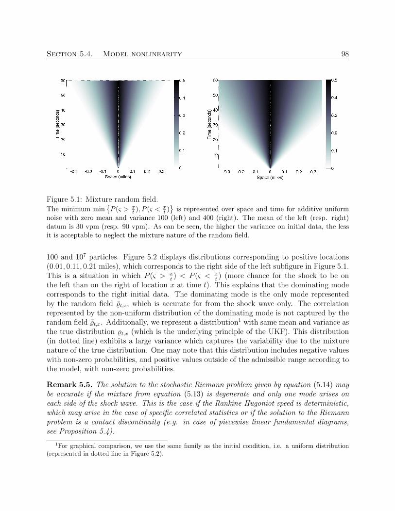
Section 5.4. Model nonlinearity 98
Figure 5.1: Mixture random field.The minimum min
P (ς > x
t ), P (ς < xt )
is represented over space and time for additive uniformnoise with zero mean and variance 100 (left) and 400 (right). The mean of the left (resp. right)datum is 30 vpm (resp. 90 vpm). As can be seen, the higher the variance on initial data, the lessit is acceptable to neglect the mixture nature of the random field.
100 and 107 particles. Figure 5.2 displays distributions corresponding to positive locations(0.01, 0.11, 0.21 miles), which corresponds to the right side of the left subfigure in Figure 5.1.This is a situation in which P (ς > x
t) < P (ς < x
t) (more chance for the shock to be on
the left than on the right of location x at time t). This explains that the dominating modecorresponds to the right initial data. The dominating mode is the only mode representedby the random field %t,x, which is accurate far from the shock wave only. The correlationrepresented by the non-uniform distribution of the dominating mode is not captured by therandom field %t,x. Additionally, we represent a distribution1 with same mean and variance asthe true distribution %t,x (which is the underlying principle of the UKF). This distribution(in dotted line) exhibits a large variance which captures the variability due to the mixturenature of the true distribution. One may note that this distribution includes negative valueswith non-zero probabilities, and positive values outside of the admissible range according tothe model, with non-zero probabilities.
Remark 5.5. The solution to the stochastic Riemann problem given by equation (5.14) maybe accurate if the mixture from equation (5.13) is degenerate and only one mode arises oneach side of the shock wave. This is the case if the Rankine-Hugoniot speed is deterministic,which may arise in the case of specific correlated statistics or if the solution to the Riemannproblem is a contact discontinuity (e.g. in case of piecewise linear fundamental diagrams,see Proposition 5.4).
1For graphical comparison, we use the same family as the initial condition, i.e. a uniform distribution(represented in dotted line in Figure 5.2).
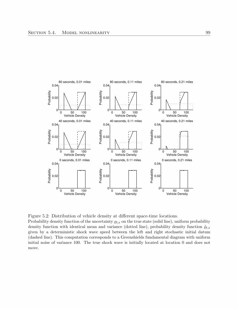
Section 5.4. Model nonlinearity 99
0 50 1000
0.02
0.04
Pro
babili
ty
Vehicle Density
80 seconds, 0.01 miles
0 50 1000
0.02
0.04
Pro
babili
ty
Vehicle Density
80 seconds, 0.11 miles
0 50 1000
0.02
0.04
Pro
babili
ty
Vehicle Density
80 seconds, 0.21 miles
0 50 1000
0.02
0.04
Pro
babili
ty
Vehicle Density
40 seconds, 0.01 miles
0 50 1000
0.02
0.04
Pro
babili
ty
Vehicle Density
40 seconds, 0.11 miles
0 50 1000
0.02
0.04
Pro
babili
tyVehicle Density
40 seconds, 0.21 miles
0 50 1000
0.02
0.04
Pro
babili
ty
Vehicle Density
0 seconds, 0.01 miles
0 50 1000
0.02
0.04
Pro
babili
ty
Vehicle Density
0 seconds, 0.11 miles
0 50 1000
0.02
0.04
Pro
babili
ty
Vehicle Density
0 seconds, 0.21 miles
Figure 5.2: Distribution of vehicle density at different space-time locations.Probability density function of the uncertainty %t,x on the true state (solid line), uniform probabilitydensity function with identical mean and variance (dotted line), probability density function %t,xgiven by a deterministic shock wave speed between the left and right stochastic initial datum(dashed line). This computation corresponds to a Greenshields fundamental diagram with uniforminitial noise of variance 100. The true shock wave is initially located at location 0 and does notmove.
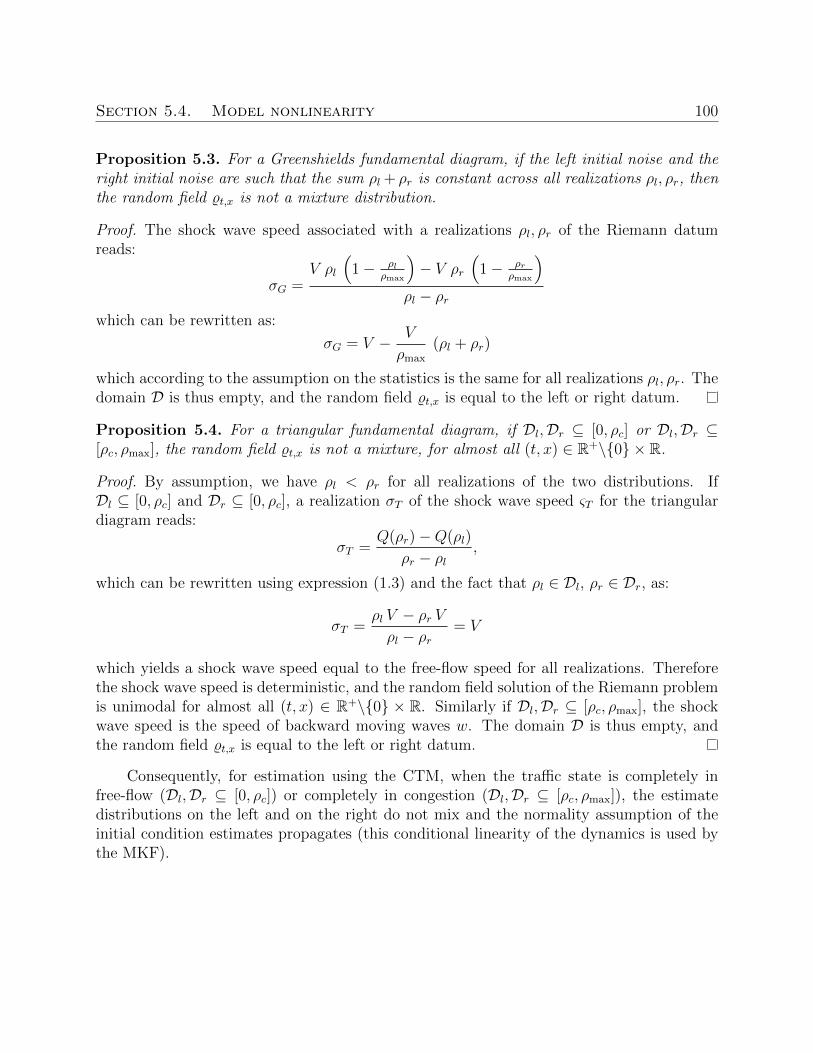
Section 5.4. Model nonlinearity 100
Proposition 5.3. For a Greenshields fundamental diagram, if the left initial noise and theright initial noise are such that the sum ρl + ρr is constant across all realizations ρl, ρr, thenthe random field %t,x is not a mixture distribution.
Proof. The shock wave speed associated with a realizations ρl, ρr of the Riemann datumreads:
σG =V ρl
(1− ρl
ρmax
)− V ρr
(1− ρr
ρmax
)ρl − ρr
which can be rewritten as:
σG = V − V
ρmax
(ρl + ρr)
which according to the assumption on the statistics is the same for all realizations ρl, ρr. Thedomain D is thus empty, and the random field %t,x is equal to the left or right datum.
Proposition 5.4. For a triangular fundamental diagram, if Dl,Dr ⊆ [0, ρc] or Dl,Dr ⊆[ρc, ρmax], the random field %t,x is not a mixture, for almost all (t, x) ∈ R+\0 × R.
Proof. By assumption, we have ρl < ρr for all realizations of the two distributions. IfDl ⊆ [0, ρc] and Dr ⊆ [0, ρc], a realization σT of the shock wave speed ςT for the triangulardiagram reads:
σT =Q(ρr)−Q(ρl)
ρr − ρl,
which can be rewritten using expression (1.3) and the fact that ρl ∈ Dl, ρr ∈ Dr, as:
σT =ρl V − ρr Vρl − ρr
= V
which yields a shock wave speed equal to the free-flow speed for all realizations. Thereforethe shock wave speed is deterministic, and the random field solution of the Riemann problemis unimodal for almost all (t, x) ∈ R+\0 × R. Similarly if Dl,Dr ⊆ [ρc, ρmax], the shockwave speed is the speed of backward moving waves w. The domain D is thus empty, andthe random field %t,x is equal to the left or right datum.
Consequently, for estimation using the CTM, when the traffic state is completely infree-flow (Dl,Dr ⊆ [0, ρc]) or completely in congestion (Dl,Dr ⊆ [ρc, ρmax]), the estimatedistributions on the left and on the right do not mix and the normality assumption of theinitial condition estimates propagates (this conditional linearity of the dynamics is used bythe MKF).
Section 5.4. Model nonlinearity 101
5.4.2 Mixture solutions to the Godunov scheme
In this section, we analyze numerically how the emergence of mixture distributions inthe solution of the Riemann problem for stochastic datum relates to the emergence of mixturedistributions in the solution to the Godunov scheme. The Godunov scheme computes anumerical solution to the Cauchy problem on a discretization grid, by iteratively solvingRiemann problems between neighboring cells and averaging their solutions within each cells.Numerical estimates produced in this manner differ from the estimates obtained by solvingthe Riemann problem on a continuous domain, due to numerical diffusion introduced in theaveraging step and the discrete setting. Additionally, in the intent of modeling numericaldiffusion, discretization error and inherent modeling error, it is common practice [131] tointroduce an additive random source term to the discretized PDE (1.5). In order to studythe emergence of mixture distributions in this context, we propose the following numericalexperiments.
We consider the Greenshields fundamental diagram with parameters V = 80 mph,ρmax = 120 vpm, and the stochastic Riemann datum (%l = N (30, 100), %r = N (90, 100)) (wetruncate the normal distribution to force its support into the admissible domain [0, ρmax] ofthe model). Using Monte Carlo simulations with 105 samples, we compute the (continuous)solution of the Riemann problem and the (discrete) solution of the Godunov scheme withCourant-Friedrichs-Lewy (CFL) [156] condition equal to one, spatially uniform left and rightrealizations of initial noise, and for various discretization grid sizes and values of the modelnoise.
Numerical diffusion: The influence of numerical diffusion on continuous and discretenumerical estimates (see Figure 5.3) is assessed by comparing the solution to the Riemannproblem (solid line) with the solution to the Godunov scheme on a coarse grid (6 space cells,18 time-steps, dashed line) and on a fine grid (12 space cells, 36 time-steps, dotted line). TheMonte Carlo simulation is run with 105 samples. As illustrated in Figure 5.3, comparison ofthe numerical solutions on different grids illustrates that diffusion in the Godunov schemesmoothens the mixture nature of the solution to the Riemann problem. The numericalsolution exhibits two modes but due to diffusion, a non-zero probability arises betweenthe two modes. This illustrates that by discretization of the constitutive model, the truenature of the distribution of uncertainty is blurred. This is not necessarily a problem if thediscrete numerical model (Godunov scheme in this case) is considered to be the physicalmodel, i.e. is considered to represent the dynamics of the true state, as commonly done intransportation. However, it show the limitation of discrete approaches for estimation withcontinuous physical models, such as the LWR PDE.
Model noise: We propose to compare (see Figure 5.4) the continuous solution to theRiemann problem (solid line), the discrete solution to the Godunov scheme with no modelnoise (dotted line), and model noise represented by a random variable N (0, 50) (dashedline), on a grid with 6 space cells, 18 time-steps. The addition of a model noise term to theGodunov scheme to account for model errors leads to a reduction of the mixture nature ofthe distribution solution to the stochastic Riemann problem. It induces a diffusion of the
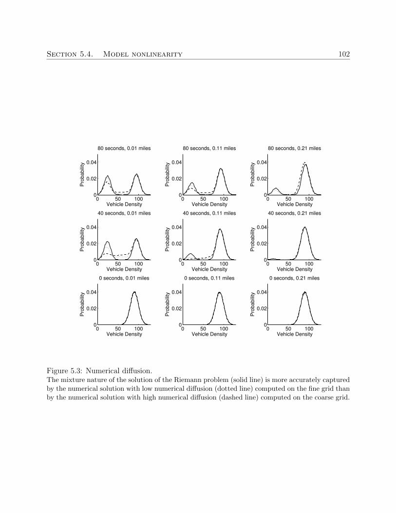
Section 5.4. Model nonlinearity 102
0 50 1000
0.02
0.04
80 seconds, 0.01 miles
Pro
babili
ty
Vehicle Density0 50 100
0
0.02
0.04
80 seconds, 0.11 miles
Pro
babili
ty
Vehicle Density0 50 100
0
0.02
0.04
80 seconds, 0.21 miles
Pro
babili
ty
Vehicle Density
0 50 1000
0.02
0.04
40 seconds, 0.01 miles
Pro
babili
ty
Vehicle Density0 50 100
0
0.02
0.04
40 seconds, 0.11 miles
Pro
babili
ty
Vehicle Density0 50 100
0
0.02
0.04
40 seconds, 0.21 miles
Pro
babili
ty
Vehicle Density
0 50 1000
0.02
0.04
0 seconds, 0.01 miles
Pro
babili
ty
Vehicle Density0 50 100
0
0.02
0.04
0 seconds, 0.11 miles
Pro
babili
ty
Vehicle Density0 50 100
0
0.02
0.04
0 seconds, 0.21 miles
Pro
babili
ty
Vehicle Density
Figure 5.3: Numerical diffusion.The mixture nature of the solution of the Riemann problem (solid line) is more accurately capturedby the numerical solution with low numerical diffusion (dotted line) computed on the fine grid thanby the numerical solution with high numerical diffusion (dashed line) computed on the coarse grid.
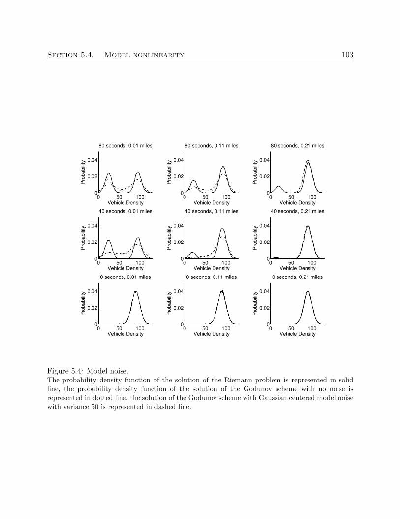
Section 5.4. Model nonlinearity 103
0 50 1000
0.02
0.04
80 seconds, 0.01 miles
Pro
babili
ty
Vehicle Density0 50 100
0
0.02
0.04
80 seconds, 0.11 miles
Pro
babili
ty
Vehicle Density0 50 100
0
0.02
0.04
80 seconds, 0.21 miles
Pro
babili
ty
Vehicle Density
0 50 1000
0.02
0.04
40 seconds, 0.01 miles
Pro
babili
ty
Vehicle Density0 50 100
0
0.02
0.04
40 seconds, 0.11 miles
Pro
babili
ty
Vehicle Density0 50 100
0
0.02
0.04
40 seconds, 0.21 miles
Pro
babili
ty
Vehicle Density
0 50 1000
0.02
0.04
0 seconds, 0.01 miles
Pro
babili
ty
Vehicle Density0 50 100
0
0.02
0.04
0 seconds, 0.11 miles
Pro
babili
ty
Vehicle Density0 50 100
0
0.02
0.04
0 seconds, 0.21 miles
Pro
babili
ty
Vehicle Density
Figure 5.4: Model noise.The probability density function of the solution of the Riemann problem is represented in solidline, the probability density function of the solution of the Godunov scheme with no noise isrepresented in dotted line, the solution of the Godunov scheme with Gaussian centered model noisewith variance 50 is represented in dashed line.

Section 5.4. Model nonlinearity 104
true distribution, which contributes to further smoothen the two components of the mix-ture (see Figure 5.4). This diffusion is more structured that pure numerical diffusion (seeFigure 5.3), but this example clearly advocates for noise modeling in order to account specif-ically for discretization error as a function of the state and the corresponding distribution ofuncertainty [121, 120, 213].
Lack of correlation: The existence of mixture distributions around the discontinu-ity creates a correlation between the two sides of the shock wave (see Figure 5.5). Bypropagating a single component of the mixture on each side of the shock wave, the covari-ance structure is misrepresented by the linearized model. This is illustrated in Figure 5.5representing the covariance structure of the estimate at time-step 20, for a Monte Carlosimulation with 104 particles in the left sub figure, and for the linearized model in the rightsub figure. The fundamental diagram is a Greenshields fundamental diagram with param-eters V = 80 mph, ρmax = 120 vpm, and the stochastic Riemann datum corresponds to(%l = N (15, 100), %r = N (75, 100)), in vehicles per mile. This corresponds to a shock-wavemoving forward, starting at time 0 from cell 0. One may note that due to the CFL condition,at time 20, no physical correlation can exist farther than 20 cells around the diagonal. Theblock diagonal structure of the linearized model estimate at the shock wave appears clearly,whereas for the Monte Carlo simulation with 104 particles, the state error covariance matrixis band diagonal, which illustrates the correlation between the two sides of the shock wavedue to the mixture components. The comparison between the two figures displays the lack ofcorrelation, across the shock, of the covariance given by the linearized model. In the absenceof correlation, measurements realized on one side of the shock do not influence the estimateon the other side of the shock. The fact that the linearized model overestimates the variancearound cells neighboring the discontinuity location is visible from the color scale.
5.4.3 Discussion
In this section, we discuss how the properties of the distribution of the uncertainty onthe true state solution of the Riemann problem with stochastic datum relate to the accuracyof the estimate given by classical filters at the analysis step.
Forecast mean: The estimate given by the mean of the distribution obtained by de-terministic propagation of the mean of the left and right datum (case of EKF), with additivemodel noise, seems biased since it only captures one component of the mixture (see Figure 5.2as well for instance). Close to the shock wave, the diffusivity of the Godunov scheme numer-ically alleviates this drawback by smoothing the mixture through diffusion. The bias at theshock wave due to mixture uncertainty is less likely to occur with sample-based filters whichimplicitly consider a stochastic model through the propagation of samples by a determin-istic model (see experiments below). We reemphasize here that the true shock wave speedfor Figure 5.2 and Figure 5.3 is zero, hence the true shock wave does not move from location 0.
Forecast variance: As illustrated in Figure 5.2, close to the shock wave, even when
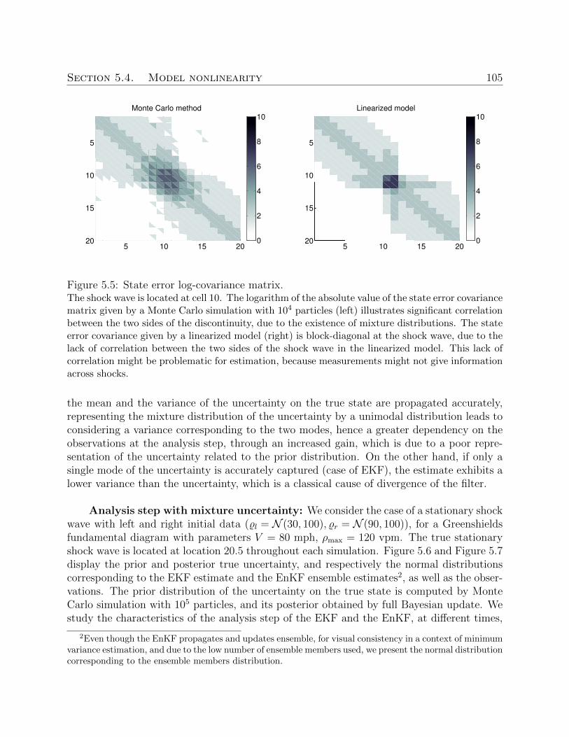
Section 5.4. Model nonlinearity 105
5
10
15
205 10 15 20
Monte Carlo method
0
2
4
6
8
10
5
10
15
205 10 15 20
Linearized model
0
2
4
6
8
10
Figure 5.5: State error log-covariance matrix.The shock wave is located at cell 10. The logarithm of the absolute value of the state error covariancematrix given by a Monte Carlo simulation with 104 particles (left) illustrates significant correlationbetween the two sides of the discontinuity, due to the existence of mixture distributions. The stateerror covariance given by a linearized model (right) is block-diagonal at the shock wave, due to thelack of correlation between the two sides of the shock wave in the linearized model. This lack ofcorrelation might be problematic for estimation, because measurements might not give informationacross shocks.
the mean and the variance of the uncertainty on the true state are propagated accurately,representing the mixture distribution of the uncertainty by a unimodal distribution leads toconsidering a variance corresponding to the two modes, hence a greater dependency on theobservations at the analysis step, through an increased gain, which is due to a poor repre-sentation of the uncertainty related to the prior distribution. On the other hand, if only asingle mode of the uncertainty is accurately captured (case of EKF), the estimate exhibits alower variance than the uncertainty, which is a classical cause of divergence of the filter.
Analysis step with mixture uncertainty: We consider the case of a stationary shockwave with left and right initial data (%l = N (30, 100), %r = N (90, 100)), for a Greenshieldsfundamental diagram with parameters V = 80 mph, ρmax = 120 vpm. The true stationaryshock wave is located at location 20.5 throughout each simulation. Figure 5.6 and Figure 5.7display the prior and posterior true uncertainty, and respectively the normal distributionscorresponding to the EKF estimate and the EnKF ensemble estimates2, as well as the obser-vations. The prior distribution of the uncertainty on the true state is computed by MonteCarlo simulation with 105 particles, and its posterior obtained by full Bayesian update. Westudy the characteristics of the analysis step of the EKF and the EnKF, at different times,
2Even though the EnKF propagates and updates ensemble, for visual consistency in a context of minimumvariance estimation, and due to the low number of ensemble members used, we present the normal distributioncorresponding to the ensemble members distribution.
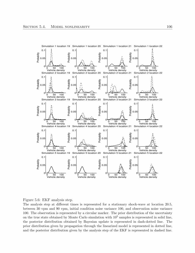
Section 5.4. Model nonlinearity 106
0 50 1000
0.05
0.1
Simulation 1 location 21
Vehicle density
Pro
babi
lty
0 50 1000
0.05
0.1
Simulation 1 location 19
Vehicle density
Pro
babi
lty
0 50 1000
0.05
0.1
Simulation 1 location 20
Vehicle densityP
roba
bilty
0 50 1000
0.05
0.1
Simulation 1 location 22
Vehicle density
Pro
babi
lty
0 50 1000
0.05
0.1
Simulation 2 location 21
Vehicle density
Pro
babi
lty
0 50 1000
0.05
0.1
Simulation 2 location 19
Vehicle density
Pro
babi
lty
0 50 1000
0.05
0.1
Simulation 2 location 20
Vehicle density
Pro
babi
lty
0 50 1000
0.05
0.1
Simulation 2 location 22
Vehicle density
Pro
babi
lty
0 50 1000
0.05
0.1
Simulation 3 location 21
Vehicle density
Pro
babi
lty
0 50 1000
0.05
0.1
Simulation 3 location 19
Vehicle density
Pro
babi
lty
0 50 1000
0.05
0.1
Simulation 3 location 20
Vehicle density
Pro
babi
lty
0 50 1000
0.05
0.1
Simulation 3 location 22
Vehicle density
Pro
babi
lty
0 50 1000
0.05
0.1
Simulation 4 location 21
Vehicle density
Pro
babi
lty
0 50 1000
0.05
0.1
Simulation 4 location 19
Vehicle density
Pro
babi
lty
0 50 1000
0.05
0.1
Simulation 4 location 20
Vehicle density
Pro
babi
lty
0 50 1000
0.05
0.1
Simulation 4 location 22
Vehicle density
Pro
babi
lty
0 50 1000
0.05
0.1
Simulation 5 location 21
Vehicle density
Pro
babi
lty
0 50 1000
0.05
0.1
Simulation 5 location 19
Vehicle density
Pro
babi
lty
0 50 1000
0.05
0.1
Simulation 5 location 20
Vehicle density
Pro
babi
lty
0 50 1000
0.05
0.1
Simulation 5 location 22
Vehicle density
Pro
babi
lty
Figure 5.6: EKF analysis step.The analysis step at different times is represented for a stationary shock-wave at location 20.5,between 30 vpm and 90 vpm, initial condition noise variance 100, and observation noise variance100. The observation is represented by a circular marker. The prior distribution of the uncertaintyon the true state obtained by Monte Carlo simulation with 105 samples is represented in solid line,the posterior distribution obtained by Bayesian update is represented in dash-dotted line. Theprior distribution given by propagation through the linearized model is represented in dotted line,and the posterior distribution given by the analysis step of the EKF is represented in dashed line.
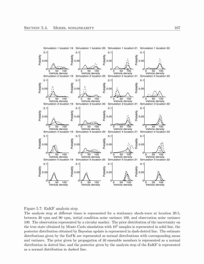
Section 5.4. Model nonlinearity 107
0 50 1000
0.05
0.1
Simulation 1 location 21
Vehicle density
Pro
babi
lty
0 50 1000
0.05
0.1
Simulation 1 location 19
Vehicle density
Pro
babi
lty
0 50 1000
0.05
0.1
Simulation 1 location 20
Vehicle densityP
roba
bilty
0 50 1000
0.05
0.1
Simulation 1 location 22
Vehicle density
Pro
babi
lty
0 50 1000
0.05
0.1
Simulation 2 location 21
Vehicle density
Pro
babi
lty
0 50 1000
0.05
0.1
Simulation 2 location 19
Vehicle density
Pro
babi
lty
0 50 1000
0.05
0.1
Simulation 2 location 20
Vehicle density
Pro
babi
lty
0 50 1000
0.05
0.1
Simulation 2 location 22
Vehicle density
Pro
babi
lty
0 50 1000
0.05
0.1
Simulation 3 location 21
Vehicle density
Pro
babi
lty
0 50 1000
0.05
0.1
Simulation 3 location 19
Vehicle density
Pro
babi
lty
0 50 1000
0.05
0.1
Simulation 3 location 20
Vehicle density
Pro
babi
lty
0 50 1000
0.05
0.1
Simulation 3 location 22
Vehicle density
Pro
babi
lty
0 50 1000
0.05
0.1
Simulation 4 location 21
Vehicle density
Pro
babi
lty
0 50 1000
0.05
0.1
Simulation 4 location 19
Vehicle density
Pro
babi
lty
0 50 1000
0.05
0.1
Simulation 4 location 20
Vehicle density
Pro
babi
lty
0 50 1000
0.05
0.1
Simulation 4 location 22
Vehicle density
Pro
babi
lty
0 50 1000
0.05
0.1
Simulation 5 location 21
Vehicle density
Pro
babi
lty
0 50 1000
0.05
0.1
Simulation 5 location 19
Vehicle density
Pro
babi
lty
0 50 1000
0.05
0.1
Simulation 5 location 20
Vehicle density
Pro
babi
lty
0 50 1000
0.05
0.1
Simulation 5 location 22
Vehicle density
Pro
babi
lty
Figure 5.7: EnKF analysis step.The analysis step at different times is represented for a stationary shock-wave at location 20.5,between 30 vpm and 90 vpm, initial condition noise variance 100, and observation noise variance100. The observation represented by a circular marker. The prior distribution of the uncertainty onthe true state obtained by Monte Carlo simulation with 105 samples is represented in solid line, theposterior distribution obtained by Bayesian update is represented in dash-dotted line. The estimatedistributions given by the EnFK are represented as normal distributions with corresponding meanand variance. The prior given by propagation of 40 ensemble members is represented as a normaldistribution in dotted line, and the posterior given by the analysis step of the EnKF is representedas a normal distribution in dashed line.
Section 5.4. Model nonlinearity 108
with a single observation with observation noise variance 100. The posterior computed bythe analysis is not propagated further but simply displayed. This means that each row inFigure 5.6 and Figure 5.7 corresponds to a a different value of the true state, a differentrealization of the observation noise, and a single analysis step. For the sake of comparisonwe always sample an observation at location 21.
The sensitivity of the filters to the observation is illustrated by the significant differencebetween the prior and the posterior (respectively dotted and dashed lines), around the shock-wave, for both the EKF and the EnKF. At the location of the observation (location 21), theprior provided by the EKF, which only captures a single mode, is more inaccurate than theprior given by the EnKF, which can account partially for mixture distributions representationwith ensemble members. However, after analysis, the posteriors for the two filters are verysimilar at the location of the observation. Away from the shock wave (location 1 and 4), itis clear that the EKF estimate exhibits a non-consistent error variance (simulations 1, 2, 3in particular).
The correlation across the shock wave clearly discriminates the two filters. Across theshock wave, at location 20, the posterior given by the EKF (dashed line) is often centered onthe wrong mode of the posterior uncertainty (dash-dotted line). This is not the case for theEnKF which captures the two modes of the mixture in most cases. When the observationcorresponds to a mode of the mixture uncertainty not well-represented by the estimate (forinstance run 2, location 21 of Figure 5.6), it can be noted that the posterior distributioncan provide more inaccurate estimate than the prior; for instance the posterior given by theEKF (dashed line) for run 2, location 20, is outside the range of values represented. Thisillustrates the difficulty to capture true correlation induced by mixture uncertainty acrossthe shock wave.
The mixture nature of the uncertainty is clearly reduced by the observation, however,the two modes are still present and propagate in the posterior uncertainty (dash-dotted lineat location 19 and 20 for simulation 1, location 22 for simulation 2, location 20 for simulation3).
These numerical examples illustrate the limitations of the suboptimal MMSE estimatesprovided by the EKF and EnKF, in the case of mixture distributions arising in traffic flowaround shock-waves. Stochastic filters such as the EnKF are more robust to the mixturenature of the uncertainty, since their sample representation allows them to better capturethe full variance of the two modes of the distribution of the uncertainty on the true state.However, this leads to higher sensitivity of the filter and may lead to instabilities at shockwaves. On the other hand, deterministic filters able to capture only a single mode of thedistribution of the uncertainty on the true state exhibit a lower variance than the uncertainty,which may cause divergence of the estimate if the models have low error terms.
Section 5.5. Model non-differentiability 109
5.5 Model non-differentiability
In this section, we show that the numerical Godunov flux defined in (1.5)- (1.6) isnon-differentiable. We prove that consequently, the discrete-time dynamics of the Godunovscheme is non-differentiable, which prevents straightforward application of filtering algo-rithms requiring differentiability to discrete transportation models based on the Godunovscheme.
5.5.1 Characterization of non-differentiability domain
The Godunov scheme consists of a dynamical system (1.5) resulting from the discretiza-tion of the transport equation where the numerical flux qG(·, ·) can be defined in a piecewisemanner on regular sub-domains in the case of a concave flux with a single maximum (1.6).The following proposition states the lack of continuous differentiability at a specific boundarybetween two of these sub-domains.
Proposition 5.5. On the domain S defined as:
S =
(ρl, ρr) ∈ [0, ρmax]2 | ρl < ρr and Q(ρl) = Q(ρr), (5.15)
the numerical Godunov flux (1.6) is not differentiable.
Proof. The expression of the numerical Godunov flux is given by equation (1.6). In eachsub-domain of definition corresponding to each line of (1.6), if the flux function Q(·) is differ-entiable, the numerical flux qG(·, ·) is also left and right differentiable. It is straightforwardto compute its left and right derivative on each sub-domain:
∂qG∂ρl
(ρl, ρr) =
Q′(ρl) if ρr ≤ ρl < ρc
0 if ρr ≤ ρc ≤ ρl
0 if ρc < ρr ≤ ρlQ′(ρl) if Q(ρl) < Q(ρr)
0 if Q(ρl) > Q(ρr)if ρl < ρr
(5.16)
∂qG∂ρr
(ρl, ρr) =
0 if ρr ≤ ρl < ρc
0 if ρr ≤ ρc ≤ ρl
Q′(ρr) if ρc < ρr ≤ ρl0 if Q(ρl) < Q(ρr)
Q′(ρr) if Q(ρl) > Q(ρr)if ρl < ρr.
(5.17)
As indicated by the fourth case of equation (5.16) (or equivalently for the right derivativewith the fourth case of equation (5.17)), the left derivative of the numerical flux is onlydefined on the left and on the right of the domain S defined by (5.15), with the left value
Section 5.5. Model non-differentiability 110
being Q′(ρl) and the right value being 0. The left and right values are equal only at thecapacity point (point of maximal flux), in the case of a flux differentiable at capacity. Sincethe left derivative is not differentiable on S, the numerical flux is not differentiable on itsdomain of definition.
The domain of non-differentiability of the numerical Godunov scheme corresponds tothe locus of stationary shock waves. In particular, the numerical Godunov flux and thediscrete dynamics associated with the Godunov scheme are differentiable at moving shockwaves. In the case of discretization schemes with higher numerical viscosity, for instance theLax-Friedrichs numerical scheme [156], differentiability is obtained everywhere but numericalapproximation of discontinuities is less accurate.
Proposition 5.6. The discrete time dynamics of the Godunov scheme is non-differentiable,and in the case of a differentiable flux function Q(·), the non-differentiability domain consistsof the locus S of stationary shock-waves.
Proof. The numerical flux is non-differentiable in the domain S defined by (5.15). Since itis impossible to have at the same time (ρni−1, ρ
ni ) ∈ S and (ρni , ρ
ni+1) ∈ S, the discrete time
dynamics defined by equation (1.5) is non-differentiable. In the case of a differentiable fluxfunction Q(·), the numerical flux is also differentiable in all its sub-domains of definition, andit can be checked in Figure 5.8 that it is also continuously differentiable at their boundaries,thus S is the non-differentiability domain of the discrete time dynamics associated with theGodunov scheme.
The non-differentiability of the discrete dynamics associated with the Godunov schemedoes not result from a numerical issue but results from the structure of the solution of thecontinuous partial differential equation considered. This can be verified by considering thesolution to the Riemann problem in the case of a stationary shock wave. The solution thatconsists of upstream and downstream densities with equal fluxes is stationary. However, itis clear that a slight perturbation of the upstream or downstream density causes the shockwave to propagate and the domain corresponding to the left or right initial condition toeventually prevail, depending on the flux balance at the discontinuity.
Remark 5.6. In the case of non-differentiable flux functions Q(·) such as the triangular fluxfunction or the Smulders flux function, it is clear that the dynamics of the numerical solutionis not differentiable. However, since the flux function results from an empirical fit, the fluxfunction can be approximated by a smooth function with relatively small consequences. Thenon-differentiability described in Proposition 5.5 results from the intrinsic properties of theconservation law, which can only by fixed by modifying the constitutive physical principles ofthe model.
Remark 5.7. For junction problems modeled as the maximization of a linear objective func-tion of the traffic state under linear inequality constraints (see Remark 1.1), the optimum isalways attained at a vertex of the constraint polytopes, hence the flow through the junction
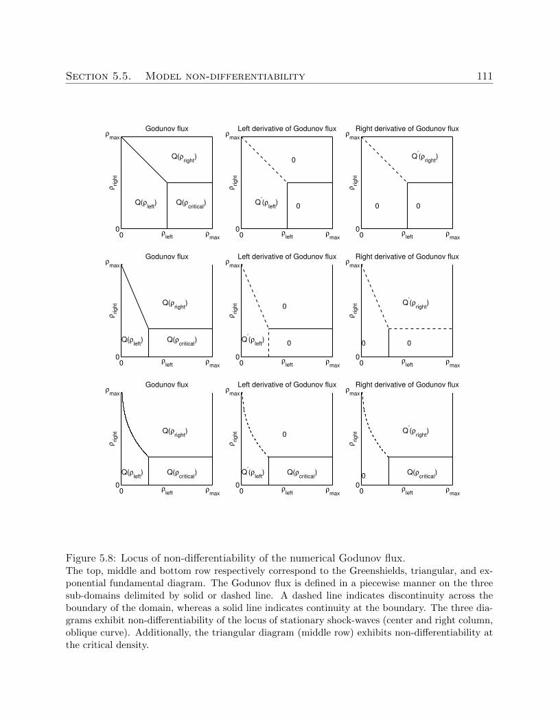
Section 5.5. Model non-differentiability 111
0 ρmax
0
ρmax
Godunov flux
ρleft
ρright
Q(ρright
)
Q(ρleft
) Q(ρcritical
)
0 ρmax
0
ρmax
Left derivative of Godunov flux
ρleft
ρright
0
Q′(ρ
left)
0
0 ρmax
0
ρmax
Right derivative of Godunov flux
ρleft
ρright
Q′(ρ
right)
0 0
0 ρmax
0
ρmax
Godunov flux
ρleft
ρright Q(ρ
right)
Q(ρleft
) Q(ρcritical
)
0 ρmax
0
ρmax
Left derivative of Godunov flux
ρleft
ρright
0
Q′(ρ
left)
0
0 ρmax
0
ρmax
Right derivative of Godunov flux
ρleft
ρright Q
′(ρ
right)
0 0
0 ρmax
0
ρmax
Godunov flux
ρleft
ρright Q(ρ
right)
Q(ρleft
) Q(ρcritical
)
0 ρmax
0
ρmax
Left derivative of Godunov flux
ρleft
ρright
0
Q′(ρ
left) Q(ρ
critical)
0 ρmax
0
ρmax
Right derivative of Godunov flux
ρleft
ρright Q
′(ρ
right)
0Q(ρ
critical)
Figure 5.8: Locus of non-differentiability of the numerical Godunov flux.The top, middle and bottom row respectively correspond to the Greenshields, triangular, and ex-ponential fundamental diagram. The Godunov flux is defined in a piecewise manner on the threesub-domains delimited by solid or dashed line. A dashed line indicates discontinuity across theboundary of the domain, whereas a solid line indicates continuity at the boundary. The three dia-grams exhibit non-differentiability of the locus of stationary shock-waves (center and right column,oblique curve). Additionally, the triangular diagram (middle row) exhibits non-differentiability atthe critical density.
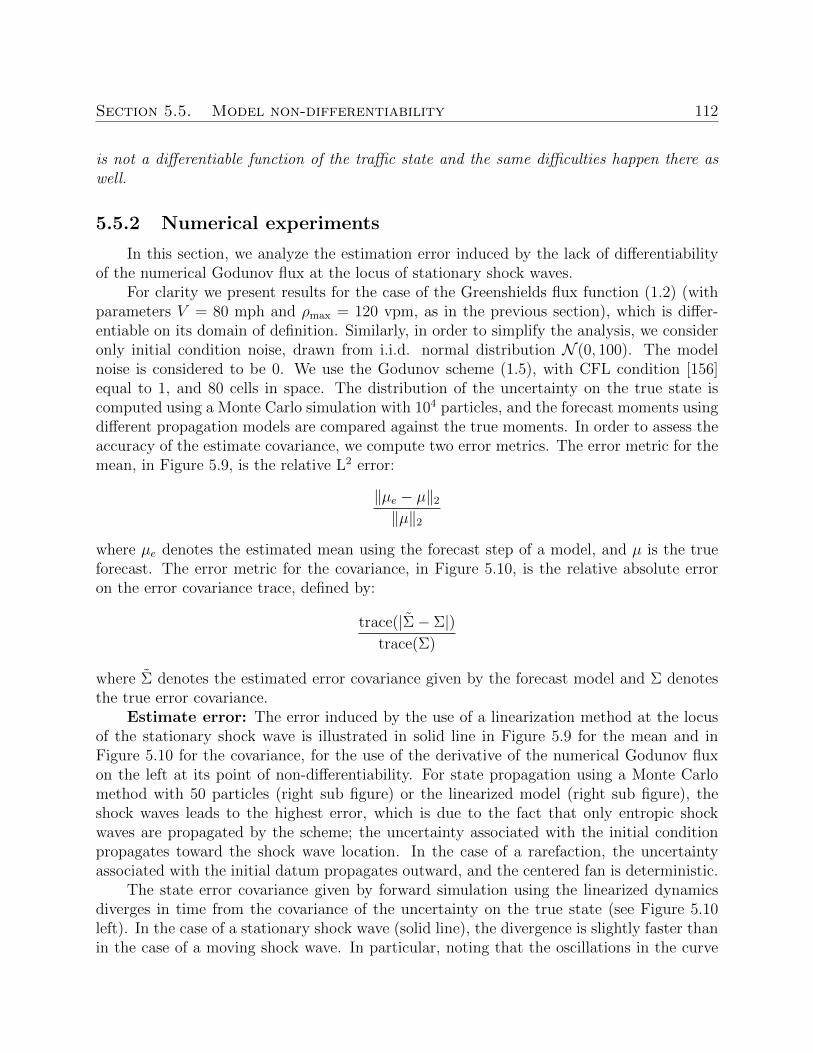
Section 5.5. Model non-differentiability 112
is not a differentiable function of the traffic state and the same difficulties happen there aswell.
5.5.2 Numerical experiments
In this section, we analyze the estimation error induced by the lack of differentiabilityof the numerical Godunov flux at the locus of stationary shock waves.
For clarity we present results for the case of the Greenshields flux function (1.2) (withparameters V = 80 mph and ρmax = 120 vpm, as in the previous section), which is differ-entiable on its domain of definition. Similarly, in order to simplify the analysis, we consideronly initial condition noise, drawn from i.i.d. normal distribution N (0, 100). The modelnoise is considered to be 0. We use the Godunov scheme (1.5), with CFL condition [156]equal to 1, and 80 cells in space. The distribution of the uncertainty on the true state iscomputed using a Monte Carlo simulation with 104 particles, and the forecast moments usingdifferent propagation models are compared against the true moments. In order to assess theaccuracy of the estimate covariance, we compute two error metrics. The error metric for themean, in Figure 5.9, is the relative L2 error:
‖µe − µ‖2
‖µ‖2
where µe denotes the estimated mean using the forecast step of a model, and µ is the trueforecast. The error metric for the covariance, in Figure 5.10, is the relative absolute erroron the error covariance trace, defined by:
trace(|Σ− Σ|)trace(Σ)
where Σ denotes the estimated error covariance given by the forecast model and Σ denotesthe true error covariance.
Estimate error: The error induced by the use of a linearization method at the locusof the stationary shock wave is illustrated in solid line in Figure 5.9 for the mean and inFigure 5.10 for the covariance, for the use of the derivative of the numerical Godunov fluxon the left at its point of non-differentiability. For state propagation using a Monte Carlomethod with 50 particles (right sub figure) or the linearized model (right sub figure), theshock waves leads to the highest error, which is due to the fact that only entropic shockwaves are propagated by the scheme; the uncertainty associated with the initial conditionpropagates toward the shock wave location. In the case of a rarefaction, the uncertaintyassociated with the initial datum propagates outward, and the centered fan is deterministic.
The state error covariance given by forward simulation using the linearized dynamicsdiverges in time from the covariance of the uncertainty on the true state (see Figure 5.10left). In the case of a stationary shock wave (solid line), the divergence is slightly faster thanin the case of a moving shock wave. In particular, noting that the oscillations in the curve
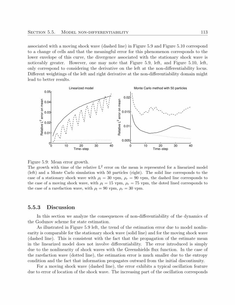
Section 5.5. Model non-differentiability 113
associated with a moving shock wave (dashed line) in Figure 5.9 and Figure 5.10 correspondto a change of cells and that the meaningful error for this phenomenon corresponds to thelower envelope of this curve, the divergence associated with the stationary shock wave isnoticeably greater. However, one may note that Figure 5.9, left, and Figure 5.10, left,only correspond to considering the derivative on the left at the non-differentiability locus.Different weightings of the left and right derivative at the non-differentiability domain mightlead to better results.
0 10 20 30 400
0.01
0.02
0.03
0.04
0.05
Re
lative
L2 e
rro
r o
n m
ea
n
Time−step
Linearized model
0 10 20 30 40
0.005
0.01
0.015
0.02
Re
lative
L2 e
rro
r o
n m
ea
n
Time−step
Monte Carlo method with 50 particles
Figure 5.9: Mean error growth.The growth with time of the relative L2 error on the mean is represented for a linearized model(left) and a Monte Carlo simulation with 50 particles (right). The solid line corresponds to thecase of a stationary shock wave with ρl = 30 vpm, ρr = 90 vpm, the dashed line corresponds tothe case of a moving shock wave, with ρl = 15 vpm, ρr = 75 vpm, the doted lined corresponds tothe case of a rarefaction wave, with ρl = 90 vpm, ρr = 30 vpm.
5.5.3 Discussion
In this section we analyze the consequences of non-differentiability of the dynamics ofthe Godunov scheme for state estimation.
As illustrated in Figure 5.9 left, the trend of the estimation error due to model nonlin-earity is comparable for the stationary shock wave (solid line) and for the moving shock wave(dashed line). This is consistent with the fact that the propagation of the estimate meanin the linearized model does not involve differentiability. The error introduced is simplydue to the nonlinearity of shock waves with the Greenshields flux function. In the case ofthe rarefaction wave (dotted line), the estimation error is much smaller due to the entropycondition and the fact that information propagates outward from the initial discontinuity.
For a moving shock wave (dashed line), the error exhibits a typical oscillation featuredue to error of location of the shock wave. The increasing part of the oscillation corresponds
Section 5.5. Model non-differentiability 114
0 10 20 30 400
0.5
1
1.5
2
Re
lative
err
or
on
err
or
co
va
ria
nce
tra
ce
Time−step
Linearized model
0 10 20 30 400
0.05
0.1
0.15
0.2
0.25
Re
lative
err
or
on
err
or
co
va
ria
nce
tra
ce
Time−step
Monte Carlo method with 50 particles
Figure 5.10: Covariance error growth.The growth with time of the relative error on the error covariance trace is represented for a linearizedmodel (left) and a Monte Carlo simulation with 50 particles (right). The solid line corresponds tothe case of a stationary shock wave with ρl = 30 vpm, ρr = 90 vpm, the dashed line correspondsto the case of a moving shock wave, with ρl = 15 vpm, ρr = 75 vpm, the dotted lined correspondsto the case of a rarefaction wave, with ρl = 90 vpm, ρr = 30 vpm.
to the mixture nature of the distribution of the uncertainty arising in the cell where the shockwave will move, hence increasing the error with the linearized model. The decreasing part ofthe oscillation corresponds to the shock wave actually propagating to the cell, and reducingthe error. The finite slope on the decreasing part corresponds to the effect of diffusion.
The non-differentiability of the numerical flux introduces an error in the error covariancewhich increases with time at a rate noticeably greater than the error growth rate in the errorcovariance for a moving shock wave (see Figure 5.10 left in which the trend of the solid lineis comparable to the trend of the top of the peaks of the dashed line).
Inaccurate estimation of the state covariance at the forecast step, depicted in Figure 5.10,impacts the use of measurements at the analysis step. This is illustrated in Figure 5.11, inwhich we consider an analysis done at time 40, for the case of the stationary shock wave,with the same parameters used in Figure 5.10. We compare the posterior error covariancecomputed by the analysis step defined by the Kalman filter (1.15), with on one hand acovariance computed by propagation of the initial condition covariance through the linearizedstate model, and on the other hand a covariance computed by a Monte Carlo simulation with104 samples. The prior means and the observations are identical for both cases, hence thediscrepancy in the posteriors is solely due to the discrepancy in the prior covariances andresult from the inaccuracy of the covariance propagated by the linearized non-differentiablemodel. A Monte Carlo simulation with 104 samples is considered to provide the distributionof the uncertainty on the true state.
As illustrated in Figure 5.11, the error associated with the prior covariance induces an
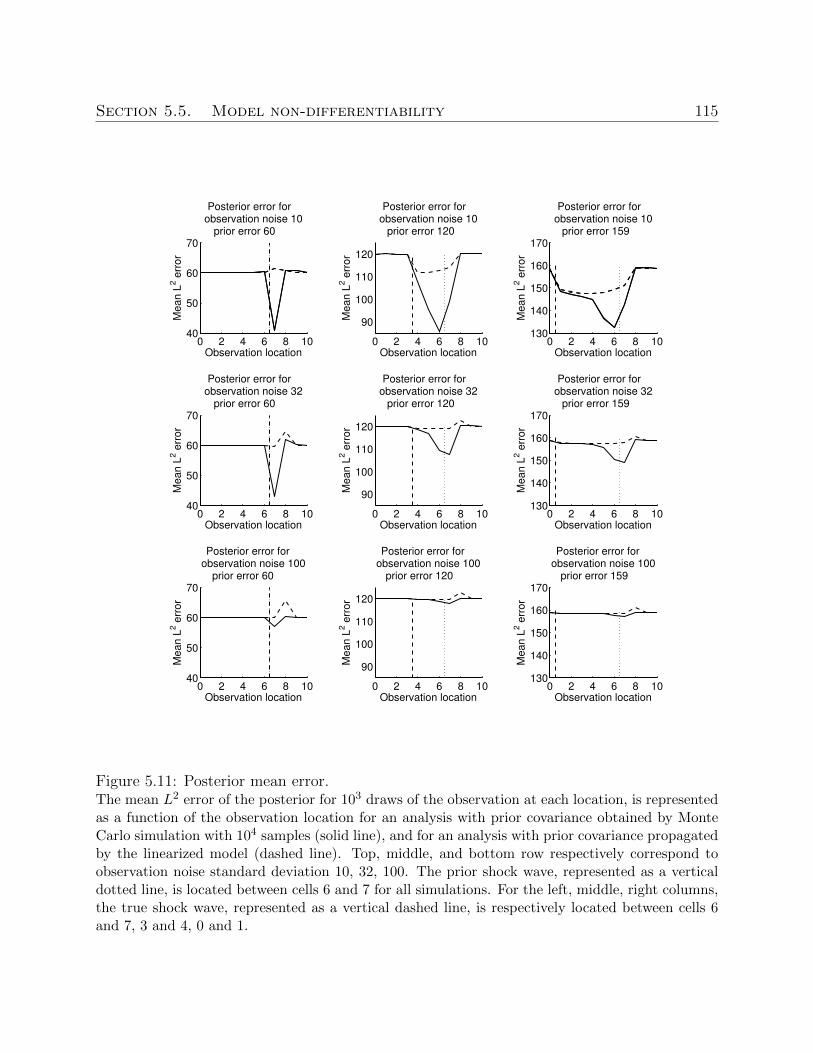
Section 5.5. Model non-differentiability 115
0 2 4 6 8 10
90
100
110
120
Observation locationM
ean L
2 e
rror
Posterior error for observation noise 10
prior error 120
0 2 4 6 8 10
90
100
110
120
Observation location
Mean L
2 e
rror
Posterior error for observation noise 32
prior error 120
0 2 4 6 8 10
90
100
110
120
Observation location
Mean L
2 e
rror
Posterior error for observation noise 100
prior error 120
0 2 4 6 8 10130
140
150
160
170
Observation location
Mean L
2 e
rror
Posterior error for observation noise 10
prior error 159
0 2 4 6 8 10130
140
150
160
170
Observation locationM
ean L
2 e
rror
Posterior error for observation noise 32
prior error 159
0 2 4 6 8 10130
140
150
160
170
Observation location
Mean L
2 e
rror
Posterior error for observation noise 100
prior error 159
0 2 4 6 8 1040
50
60
70
Observation location
Mean L
2 e
rror
Posterior error for observation noise 10
prior error 60
0 2 4 6 8 1040
50
60
70
Observation location
Mean L
2 e
rror
Posterior error for observation noise 32
prior error 60
0 2 4 6 8 1040
50
60
70
Observation location
Mean L
2 e
rror
Posterior error for observation noise 100
prior error 60
Figure 5.11: Posterior mean error.The mean L2 error of the posterior for 103 draws of the observation at each location, is representedas a function of the observation location for an analysis with prior covariance obtained by MonteCarlo simulation with 104 samples (solid line), and for an analysis with prior covariance propagatedby the linearized model (dashed line). Top, middle, and bottom row respectively correspond toobservation noise standard deviation 10, 32, 100. The prior shock wave, represented as a verticaldotted line, is located between cells 6 and 7 for all simulations. For the left, middle, right columns,the true shock wave, represented as a vertical dashed line, is respectively located between cells 6and 7, 3 and 4, 0 and 1.
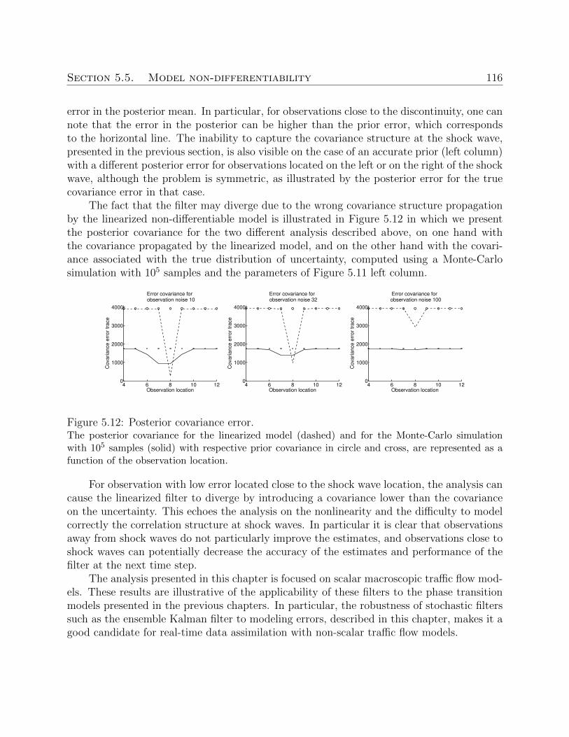
Section 5.5. Model non-differentiability 116
error in the posterior mean. In particular, for observations close to the discontinuity, one cannote that the error in the posterior can be higher than the prior error, which correspondsto the horizontal line. The inability to capture the covariance structure at the shock wave,presented in the previous section, is also visible on the case of an accurate prior (left column)with a different posterior error for observations located on the left or on the right of the shockwave, although the problem is symmetric, as illustrated by the posterior error for the truecovariance error in that case.
The fact that the filter may diverge due to the wrong covariance structure propagationby the linearized non-differentiable model is illustrated in Figure 5.12 in which we presentthe posterior covariance for the two different analysis described above, on one hand withthe covariance propagated by the linearized model, and on the other hand with the covari-ance associated with the true distribution of uncertainty, computed using a Monte-Carlosimulation with 105 samples and the parameters of Figure 5.11 left column.
4 6 8 10 120
1000
2000
3000
4000
Observation location
Covariance e
rror
trace
Error covariance for
observation noise 100
4 6 8 10 120
1000
2000
3000
4000
Observation location
Covariance e
rror
trace
Error covariance for
observation noise 32
4 6 8 10 120
1000
2000
3000
4000
Observation location
Covariance e
rror
trace
Error covariance for
observation noise 10
Figure 5.12: Posterior covariance error.The posterior covariance for the linearized model (dashed) and for the Monte-Carlo simulationwith 105 samples (solid) with respective prior covariance in circle and cross, are represented as afunction of the observation location.
For observation with low error located close to the shock wave location, the analysis cancause the linearized filter to diverge by introducing a covariance lower than the covarianceon the uncertainty. This echoes the analysis on the nonlinearity and the difficulty to modelcorrectly the correlation structure at shock waves. In particular it is clear that observationsaway from shock waves do not particularly improve the estimates, and observations close toshock waves can potentially decrease the accuracy of the estimates and performance of thefilter at the next time step.
The analysis presented in this chapter is focused on scalar macroscopic traffic flow mod-els. These results are illustrative of the applicability of these filters to the phase transitionmodels presented in the previous chapters. In particular, the robustness of stochastic filterssuch as the ensemble Kalman filter to modeling errors, described in this chapter, makes it agood candidate for real-time data assimilation with non-scalar traffic flow models.
117
Chapter 6
Boundary stabilization of weaksolutions to scalar conservation laws
In this chapter, we consider the problem of stabilization of systems modeled by scalarhyperbolic conservation laws. This applies directly to traffic modeling with the LWR model,and to fluid-dynamic models with the Burgers equation. We assume that the actuators ofthe system are located at the boundaries. In particular, for transportation networks, thisproblem setting can be understood as the problem of the design of variable speed limits orramp metering.
The problem of boundary control of partial differential equations has been the focus ofsustained research. A large volume of literature is concerned with the problem of boundarycontrol of the viscous Burgers equation. Control results can be found in [43, 44, 138, 139,165, 200]. A Lyapunov approach, from which the method presented in this chapter wasinspired, has been proposed in [139], for classical solutions to the PDE.
Lyapunov methods for classical solutions of networks of scalar conservation laws havealso been proposed in [18], and for classical solutions of 2 × 2 systems with characteristicsspeeds of constant opposite sign in [64, 81]. Similar work on boundary damping techniqueswith applications to the Saint-Venant equations has been proposed in [75, 187]. Switchingtechniques for linear hyperbolic systems are investigated in [6, 7]. A frequency domainframework [161] has been used to design a boundary control for the linearized Saint-Venantequations in [162] (see also [108] for boundary control of the Saint-Venant equations). Aspecific method for flat systems has been introduced in [95] (see also [186] in the context ofthe Burgers equation).
Methods developed specifically for well-posedness results of conservation laws have alsobeen applied to the problem of boundary control. In [8], a wavefront tracking method wasused to compute the fixed horizon attainable set of initial-boundary value problem solutionsof Temple systems of conservation laws.
Frameworks arising from the field of optimal control have also been applied to thisproblem [123, 122]. In [12], the authors proposed a viability framework for a Hamilton-Jacobiequation corresponding to an integral form of the Burgers equation, which leads to lower
Section 6.1. Problem statement 118
semi-continuous solutions. A linear relaxation method for the nonlinear discrete dynamicsof the asymmetric cell-transmission model, a specific instantiation of the Godunov schemefor the LWR equation, has also been proposed in [104], with subsequent global optimizationof the obtained equivalent convex problem. In the context of network traffic and dynamictraffic assignment, we refer the reader to [185] and the references therein. The problem ofair traffic flow control has been notably addressed using adjoint methods in [20] and in [226]using a convex formulation.
One of the challenging features of conservation laws is the apparition of discontinuitiesin finite time in the solution to the Cauchy problem, even for smooth initial condition. Thisyields difficulties for most control approaches since classical control methods are not well-suited to handle discontinuities. In the case of parametric initial conditions, the problem ofdifferentiating the solution to the scalar conservation law with respect to the initial conditionparameter has been specifically addressed in [16] from a mathematical perspective. One mustalso note the more general shift differentiability method for functionals on L1∩BV introducedin [22, 41] (see section 6.2.1 for a definition of the class of BV functions).
A second specific challenge of boundary control of the solution to a conservation lawalso due to the non-linearity of the PDE is the fact that weak boundary conditions haveto be considered. In this work, we specifically account for these two issues and show thestability of the weak entropy solution to the scalar conservation law (6.1).
6.1 Problem statement
Consider the scalar conservation law in one dimension of space
∂tu+ ∂xf(u) = 0 (6.1)
in the domain Ω.= (t, x)| t ≥ 0 and a ≤ x ≤ b. The flux function f(·) is assumed to be
smooth and strictly convex. The initial-boundary value problem (IBVP) for (6.1) in Ω withinitial condition u0 : (a, b) 7→ R, and boundary conditions ua, ub : R+ 7→ R, reads
∂tu+ ∂xf(u) = 0 (6.2)
u(0, x) = u0(x) (6.3)
u(t, a) = ua(t), u(t, b) = ub(t). (6.4)
The Lyapunov boundary stabilization problem can be formulated as follows.
Definition 6.1. Given a stationary solution u∗ to the PDE (6.1), and an initial conditionu0 with bounded variations (see section 6.2.1), the Lyapunov (resp. asymptotic) boundarystabilization problem consists in the existence of boundary conditions ua, ub such that theIBVP (6.2)-(6.3)-(6.4) is well-posed and its solution is (resp. asymptotically) stable in thesense of Lyapunov at u∗.
Section 6.2. Preliminaries 119
Stationary solutions to the PDE include uniform solutions and solutions with a singlestationary jump discontinuity. We address the case of uniform solutions in Section 6.4.
The well-posedness of the IBVP (6.2)-(6.3)-(6.4) is critical to the definition of theproblem, since the design of arbitrary boundary conditions can make the problem ill-posed(see [205] for an illustration on the LWR equation in the case of traffic). This would lead toa discrepancy between the control implemented and its realized value in the system, and adivergence between the desired trajectory of the system and its real trajectory. In the caseof traffic, it corresponds for instance to installing a green traffic light at the location of atraffic jam with the intended goal that cars in the jam adopt the corresponding free-flowspeed. For well-posedness of the IBVP (6.2)-(6.3)-(6.4), the PDE (6.1) and the boundaryconditions (6.4) must be understood in the weak sense. The weak formulation is presentedin Section 6.2.2.
6.2 Preliminaries
In this section, we introduce the notations and classical results subsequently usedthroughout this chapter.
6.2.1 BV functions
Consider an interval J ⊂ R, and a map u : J 7→ R. The total variation of u is definedas
Tot. Var. u .= sup
N∑i=1
|u(xj)− u(xj−1)|
(6.5)
where the supremum is taken over all N ≥ 1 and all (N + 1)-tuples of points xj ∈ J suchthat x0 < x1 < . . . < xN . If the total variation of u is finite, u ∈ BV . Specific properties ofBV functions leveraged in the following sections are presented below1.
Lemma 6.1. [39] Let u : (a, b) 7→ Rn have bounded variations. Then for every x ∈ (a, b),the left and right limits
u(x−).= lim
y 7→x−u(y), u(x+)
.= lim
y 7→x+u(y)
are well defined. Moreover, u has at most countably many points of discontinuity.
The following lemma concerns piecewise constant approximability of BV functions.
Lemma 6.2. [39] Let u : R 7→ Rn be right continuous with bounded variations. Then, forevery ε > 0, there exists a piecewise constant function v such that:
Tot. Var. v ≤ Tot. Var. u , ‖v − u‖L∞ ≤ ε.
1Proofs of these properties can be found in section 2.4 of [39].
Section 6.2. Preliminaries 120
If, in addition, ∫ 0
−∞|u(x)− u(−∞)| dx+
∫ +∞
0
|u(x)− u(∞)| dx <∞,
then one can find v with the additional property
‖u− v‖L1 ≤ ε.
The space of BV functions and its closure in L1 are at the center of well-posednessresults for conservation laws using wavefront-tracking methods.
6.2.2 Weak solutions to the initial-boundary value problem
It is well-known that approximate jump discontinuities can arise in finite time in so-lutions to conservation laws [89]. Thus classical solutions do not exist in general, and it isnecessary to consider a more general formulation of the conservation law.
Weak entropy solution to the Cauchy problem
The weak formulation of the conservation law is obtained by considered derivatives inthe sense of distribution.
Definition 6.2. A function u : [0, T ] × R 7→ R is a weak solution to the Cauchy prob-lem (6.2)-(6.3) if the initial condition (6.3) is satisfied, and if additionally, for any continu-ously differentiable function φ with compact support contained in (−∞, T )× R,∫ T
0
∫ ∞−∞
(uφt + f(u)φx) dx dt+
∫ ∞−∞
u0(x)φ(0, x)dx = 0, (6.6)
and t 7→ u(t, ·) is continuous from [0, T ] into L1loc.
When integrated in a domain in which u is smooth around an approximate jump dis-continuity, the weak formulation (6.6) yields the Rankine-Hugoniot relation [89] defining thespeed σ of propagation of approximate jump discontinuities
σ∆u = ∆f(u), (6.7)
where ∆u = ur − ul is the jump in u, with ur, ul the right and left values of u, respectively,at the approximate jump discontinuity.
For uniqueness of the solution to the weak solution of the Cauchy problem associatedwith the conservation law, an additional admissibility condition (see Section 4.5 of [70]) isrequired. Different conditions have been proposed in literature. In the scalar case, one ofthe first admissibility conditions is due to Oleinik [180]. Kruzkhov [141] showed that it wassufficient to satisfy the entropy inequality condition for a specific family of entropy-entropy
Section 6.2. Preliminaries 121
flux pairs in the scalar case, yielding the Kruzkhov entropy condition. The Lax admissibilitycondition [147], which exhibits a convenient geometric interpretation, states that for a i-shockjoining a left state ul and a right state ur, the following inequality must be satisfied:
λi(ul) ≥ σ ≥ λi(ur) (6.8)
where λi(u) is the ith characteristic speed of u, and σ is the Rankine-Hugoniot speed (6.7).In the scalar case, for a convex flux, these formulations have been proven to be equivalent(see Section 2.1 of [154]). The Lax admissibility condition allows the selection of a particularweak solution.
Definition 6.3. A function u : [0, T ]× R 7→ R is the weak entropy solution to the Cauchyproblem (6.2)-(6.3) if it is a weak solution (definition 6.2), that satisfies the Lax admissibilitycondition (6.8).
The definition of weak conditions to the IBVP requires a corresponding statement ofweak boundary conditions, presented in the following section.
Weak boundary conditions
The first statement of weak boundary conditions was introduced in [15] in the scalarcase in multiple dimensions of space, with C2 flux and C2 initial and boundary datum, usinga vanishing viscosity method. In one dimension, this formulation reads:
maxk∈[α,β]
sgn (u(t, a)− ua(t)) (f(u(t, a))− f(k)) = 0 (6.9)
mink∈[γ,δ]
sgn (u(t, b)− ub(t)) (f(u(t, b))− f(k)) = 0 (6.10)
for almost all t > 0, and where α = min(u(t, a), ua(t)), β = max(u(t, a), ua(t)), γ =min(u(t, b), ub(t)), δ = max(u(t, b), ub(t)), and sgn denotes the sign function. This formula-tion was shown to hold for systems of conservation laws in one dimension of space in [82],and proven equivalent to a formulation derived from the solution to the Riemann problemat the boundary, later extended to account for continuous boundary not necessarily staticin [3]. In the scalar case, at a left boundary a, the statement of weak boundary conditionsderived from the structure of the solution to the Riemann problem is the following.
Definition 6.4. A function u : Ω 7→ R satisfies the boundary condition ua at a if for allexcept countably many times t, the waves composing the solution to the Riemann problemcentered at a with initial data
ua(t) if x < a
u(t, a) if x > a(6.11)
have negative speeds.
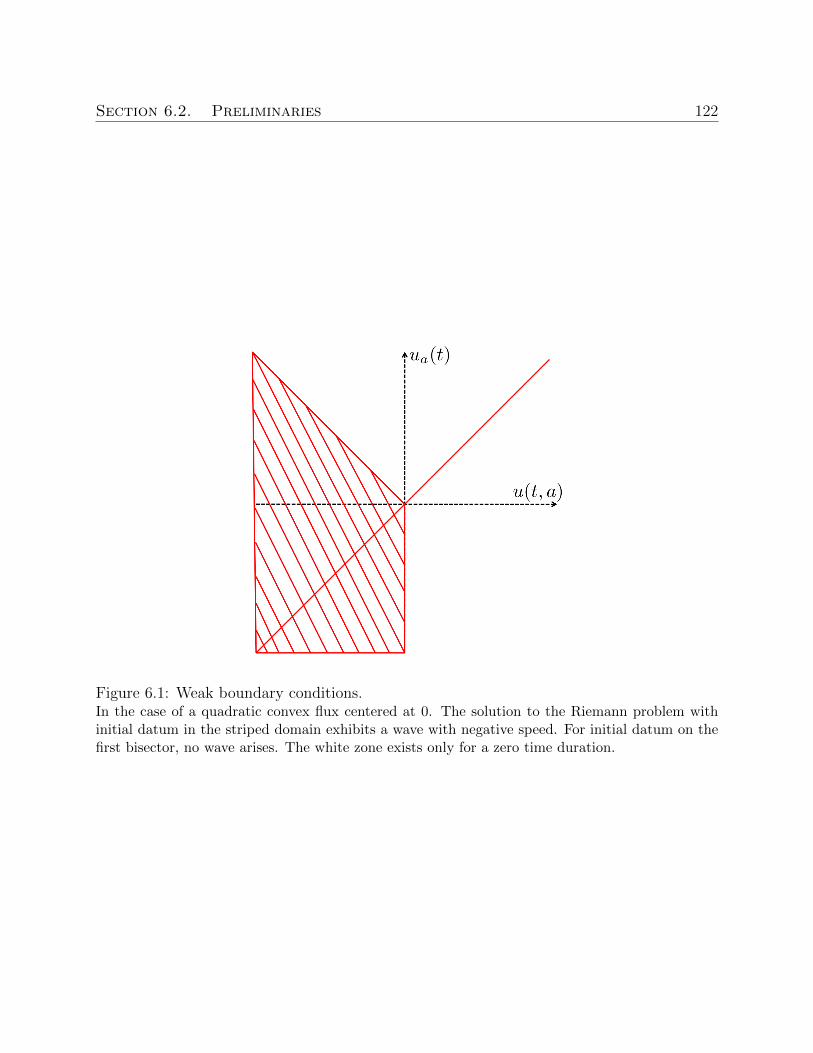
Section 6.2. Preliminaries 122
Figure 6.1: Weak boundary conditions.In the case of a quadratic convex flux centered at 0. The solution to the Riemann problem withinitial datum in the striped domain exhibits a wave with negative speed. For initial datum on thefirst bisector, no wave arises. The white zone exists only for a zero time duration.
Section 6.2. Preliminaries 123
The domain for which the couples boundary condition-boundary trace prevail for anon-zero duration, (definition 6.4) is represented in figure 6.1 for a Burgers flux.
In [153], a simplified formulation is proposed for the scalar case with strictly convexcontinuously differentiable flux functions (see also [96]). Similar formulations were derivedfor a scalar traffic model in [205] and scalar traffic models on networks with application toestimation in [227], following [97]. In the case of a strictly convex continuously differentiableflux, this statement states that for almost all times t, one of the following mutually exclusiveconditions must be satisfied:
u(t, a) = ua(t)
f ′(u(t, a)) ≤ 0 and f ′(ua(t)) ≤ 0 and u(t, a) 6= ua(t)
f ′(u(t, a)) ≤ 0 and f ′(ua(t)) > 0 and f(u(t, a)) ≥ f(ua(t)).
(6.12)
The same can be done at the downstream boundary x = b:u(t, b) = ub(t)
f ′(u(t, b)) ≥ 0 and f ′(ub(t)) ≥ 0 and u(t, b) 6= ub(t)
f ′(u(t, b)) ≥ 0 and f ′(ub(t)) < 0 and f(u(t, b)) ≥ f(ub(t)).
(6.13)
A well-posedness result for the IBVP associated with a scalar conservation law (6.1) withthe boundary statement from definition 6.4 is presented in the following section.
6.2.3 Well-posedness of the initial-boundary value problem
In [15], a solution satisfying (6.6) in the scalar case is contructed using a vanishingviscosity method for the weak boundary conditions statement (6.9)-(6.10) and is shown tobe the admissible solution according to Kruzkhov entropy condition [141].
More recently, an existence result for n× n systems using wavefront tracking was pro-posed in [3]. The standard Riemann semigroup (SRS) method, introduced in [38] for theCauchy problem associated with a Temple system [210] of conservation laws, was extendedto the IBVP in [4, 5], with the boundary conditions statement from definition 6.4. In [5], itis shown for a n × n system that if the SRS exist, its trajectories coincide with wavefronttracking solutions. Uniqueness and continuous dependence is obtained for the case of non-characteristic conditions, and uniqueness for the characteristic case. The SRS is constructedfor 2×2 system in [4]. We state in the scalar case for a static boundary the main result of [4]for characteristic boundary conditions, obtained for 2×2 systems with continuous boundary(see theorem C of [4]).
Theorem 6.1. [4] Let f be a smooth map such that the system (6.1) is strictly hyperbolicwith characteristic field linearly degenerate or genuinely nonlinear. There exists positiveconstants L and δ, and a continuous semigroup S defined for data in L1 ∩ BV with totalvariation bounded by δ, such that
Section 6.3. Approximation of solution 124
• The map t 7→ u(t, ·) yields a solution to the IBVP (6.6)-(6.3)-(6.11).
• For piecewise constant initial and boundary data, the trajectories of the semigroup co-incide with the solution to the IBVP obtained by piecing together the standard solutionsto the Riemann problems at the points of discontinuity of the initial condition and atthe boundary.
• For initial data u′0, u′′0, boundary data u′a = u′′a in L1 ∩BV with total variation bounded
by δ, let u′, u′′ denote the corresponding trajectories of the semigroup S, and t′, t′′ > 0,then
‖u′(t′, ·)− u′′(t′′, ·)‖1 ≤ L (‖u′0 − u′′0‖1) . (6.14)
In the following section we use this result in the case of a left and a right boundary toshow that we can restrict our Lyapunov analysis to the case of piecewise smooth data.
6.3 Approximation of solution
In this section, we present results on the approximability of the solution to an initial-boundary value problem (IBVP) with initial condition in BV by the solution to an IBVPwith piecewise smooth solution at all times. We show that the solution to the IBVP withBV data can be approximated arbitrarily closely in the L1 norm by the solution to an IBVPwith piecewise smooth data. We define the required regularity class used throughout thechapter.
Definition 6.5. We note PWS+ the class of piecewise smooth functions f : R 7→ R suchthat the gradient g of f satisfies the following properties:
• g is positive almost everywhere.
• there is a finite number of locations at which g is a negative Dirac mass.
We now state the approximability result.
Theorem 6.2. Let T, δ > 0, a < b, and let u0 : (a, b) 7→ R, ua, ub : (0, T ) 7→ R be functionswith total variation bounded by δ. For every ε > 0, there exists uε0 : (a, b) 7→ R in PWS+
such that the solution u to the IBVP for equation (6.1) and data (u0, ua, ub) and the solutionuε to the IBVP for equation (6.1) and data (uε0, ua, ub) satisfy:
∀ 0 ≤ t ≤ T, ‖u(t, ·)− uε(t, ·)‖1 ≤ ε.
Proof. Using lemma 6.2 in the compact domain [a, b], we can approximate the initial con-dition condition u0 approximated arbitrarily closely in the L1 sense by a piecewise constantfunction uε0 with a finite number of discontinuities and lower total variation.
Using the continuous dependence result of theorem 6.1, the resulting trajectories u, uεof the semigroup for the identical boundary conditions ua, ub, can be made arbitrarily closein the L1 norm by controlling the distance between the initial conditions.
Section 6.4. Lyapunov analysis 125
Remark 6.1. It is clear that approximating the problem data by piecewise constant datasatisfies the requirements of theorem 6.2. However, the class of piecewise constant data isnot close for the semigroup. In the case of wavefront tracking, the propagation of piecewiseconstant conditions is achieved by introduction of non-entropic shock waves. As shown insection 6.4, the entropy condition is a critical component of the stability of the solution to theIBVP. Hence we work in the class of piecewise smooth functions, that allows approximationsof BV function, as proven in theorem 6.2, and is close for the semigroup as proven intheorem 6.3.
We show that under suitable boundary conditions, the solution to the IBVP with piece-wise smooth data is piecewise smooth.
Theorem 6.3. Let T, δ > 0, a < b, and let u0 : (a, b) 7→ R, ua, ub : (0, T ) 7→ R be in PWS+.Let u denote the solution to the IBVP (6.6)-(6.3)-(6.11). At all times 0 ≤ t ≤ T , u(t, ·) ispiecewise smooth.
Proof. Let x1, . . . , xN denote the locations of the discontinuities in the initial condition,including a, b. We construct the solution to the IBVP by piecing together the shock wavesor rarefaction waves created at xi, and the classical solution constructed by the methodof characteristics between the waves. By definition, the solution created is a solution inthe sense of (6.6) since equation (6.1) is satisfied in the classical sense between the waves,and the shock waves propagate according to the Rankine-Hugoniot relation (6.7). It is alsothe admissible solution according to the Lax condition (6.8) by enforcing the existence ofentropic shock waves only. Finally the constructed solution coincides with the trajectory ofthe semigroup from theorem 6.2 (see [40]).
We now show that at all time, the number of discontinuities is finite. Since there isa finite number of discontinuities in the initial and boundary conditions, a finite numberof discontinuities enters the space-time domain. In the scalar case the interaction of twodiscontinuities creates no more than one discontinuity, so the interaction of discontinuitiescontributes to decreasing their number. Finally as mentioned above, since the initial andboundary conditions are piecewise smooth increasing, all discontinuities are created at time0 or at the boundary.
In the next section, we present the Lyapunov stability analysis for functions in PWS+.
6.4 Lyapunov analysis
In this section, we propose a Lyapunov function and compute its derivative. In thefollowing we call u = u− u∗ where u∗ is a uniform, hence stationary, solution around whichwe want to stabilize the system, and u is the solution to the IBVP associated with the scalarconservation law (6.1). Following the results from section 6.3, we assume that u is in PWS+.
Section 6.4. Lyapunov analysis 126
6.4.1 Lyapunov function candidate
We consider the classical Lyapunov function candidate [139, 140]:
V (t) =
∫ b
a
u2(x, t) dx. (6.15)
where u is a weak solution to the scalar conservation law. From definition 6.3, we havet 7→ u(t, ·) continuous from [0, T ] to L1, and the function V (·) is well-defined and continuous.We index the jump discontinuities of u(t, ·) in increasing order of their location at time t byi = 0, . . . , N(t), including for notational purposes the boundaries a, b, with x0(t) = a andxN(t) = b. The Lyapunov function candidate can be rewritten as:
V (t) =1
2
N(t)−1∑i=0
∫ xi+1(t)
xi(t)
u2(t, x) dx. (6.16)
From theorem 6.3, we know that for all integer i ∈ [0, N(t)), the function u(t, ·) is smoothin the domain (xi(t), xi+1(t)), thus ∂tu(t, ·) exists and is continuous for t such that xi(t) <xi+1(t). Since discontinuity trajectories are differentiable with speed given by the Rankine-Hugoniot relation (6.7), it follows that at any time t such that N(t) is constant in a neigh-borhood of t and the boundary trace is continuous, the function V (·) is differentiable.
6.4.2 Differentiation of the Lyapunov function candidate
In this section, we compute the derivative of the Lyapunov function candidate (6.15),at any time t such that N(t) is constant in a neighborhood and the boundary trace iscontinuous. Differentiating expression (6.16) yields:
dV
dt(t) =
1
2
N(t)−1∑i=0
∫ xi+1(t)
xi(t)
∂tu2 dx+
1
2
N(t)−1∑i=0
[u2(t, xi+1(t)−)
dxi+1
dt(t)− u2(t, xi(t)+)
dxidt
(t)
].
(6.17)
As detailed at the end of section 6.4.1, the term under the sum is smooth, and we can write∂tu
2 = 2 u ∂tu. Since u satisfies the conservation law (6.1), we have ∂tu = −∂xf(u + u∗).The derivative of the Lyapunov function can be written as:
dV
dt(t) =−
N(t)−1∑i=0
∫ xi+1(t)
xi(t)
u ∂xf(u+ u∗) dx
+1
2
N(t)−1∑i=0
[u2(t, xi+1(t)−)
dxi+1
dt(t)− u2(t, xi(t)+)
dxidt
(t)
].
Section 6.4. Lyapunov analysis 127
By integrating by parts the sum terms, we obtain:
dV
dt(t) =−
N(t)−1∑i=0
[u f(u+ u∗)]xi+1(t)xi(t)
+
N(t)−1∑i=0
∫ xi+1(t)
xi(t)
f(u+ u∗) ∂xu dx
+1
2
N(t)−1∑i=0
[u2(t, xi+1(t)−)
dxi+1
dt(t)− u2(t, xi(t)+)
dxidt
(t)
].
and if we note F (·) a primitive function of the flux function f(·) we have:
dV
dt(t) = u(t, a) f(u(t, a) + u∗)− u(t, b) f(u(t, b) + u∗)− F (u(t, a) + u∗) + F (u(t, b) + u∗)
+
N(t)−1∑i=1
[∆i (uf(u+ u∗)− F (u+ u∗))− 1
2
dxidt
(t) ∆i u2
],
where ∆i is defined around the discontinuity xi(t) as in equation (6.7). Using the Rankine-Hugoniot relation, defined in equation (6.7), to write the speed of the approximate jumpdiscontinuity dxi(t)/dt as a function of the left and right jump values we obtain:
dV
dt(t) = u(t, a) f(u(t, a) + u∗)− u(t, b) f(u(t, b) + u∗)− F (u(t, a) + u∗) + F (u(t, b) + u∗)
+
N(t)−1∑i=1
∆i (uf(u+ u∗)− F (u+ u∗))−N(t)−1∑i=1
u(t, xi−) + u(t, xi+)
2∆if(u+ u∗).
(6.18)
In equation (6.18) we identify the first four terms that depend on the boundary trace of thesolution, and the last two terms that depend on the shock dynamics inside the domain. Inthe following section, we analyze the stability properties of the internal terms.
6.4.3 Internal stability
The last two terms of equation (6.18) correspond to approximate jump discontinuity inthe solution and are neither observable nor controllable from the boundaries. We now showthat these terms have a stabilizing effect on the Lyapunov function candidate (6.15).
Proposition 6.1. Given a uniform stationary solution u∗ to the scalar conservation law (6.1),the approximate jump discontinuity dynamics
N(t)−1∑i=1
[∆i (uf(u+ u∗)− F (u+ u∗)) − u(t, xi−) + u(t, xi+)
2∆if(u+ u∗)
](6.19)
of the solution u to the IBVP, contributes to the decrease of the Lyapunov function candi-date (6.15).
Section 6.4. Lyapunov analysis 128
Proof. In order to show that the term (6.19) is negative, we show that each term in the sumis negative. If we note ul, ur the value of u on the left and on the right of the approximatejump discontinuity, respectively, and ul, ur the corresponding reduced variables, we want toshow that
[(urf(ur + u∗)− F (ur + u∗))− (ulf(ul + u∗)− F (ul + u∗))]
− ul + ur2
(f(ur + u∗)− f(ul + u∗)) ≤ 0.
Equivalently, in the original state variable u = u+ u∗, we have:
[((ur − u∗) f(ur)− F (ur))− ((ul − u∗) f(ul)− F (ul))]
− ul + ur − 2u∗
2(f(ur)− f(ul)) ≤ 0.
This can be rewritten as:
F (ul)− F (ur) +1
2(ur − ul) (f(ur) + f(ul)) ≤ 0, (6.20)
in which we recognize Oleinik entropy condition [180]. Thus we have equivalence betweenstability of the approximate jump discontinuity dynamics and Oleinik entropy condition.
Remark 6.2. From the equivalence with the Oleinik entropy condition, since the flux func-tion is strictly convex, we see that the internal dynamics is strictly stabilizing (no contactdiscontinuity).
Remark 6.3. When the number of shocks is constant inside the domain and the trace of thesolution is continuous, the internal dynamics is stabilizing in the sense that it contributes tothe decay of the Lyapunov function candidate (6.15). Since the Lyapunov function candidateis continuous, the internal dynamics is always stabilizing. This is critical for boundarystabilization where the control action cannot apply directly inside the domain (unlike the caseof distributed control [79, 87, 157]). From equation (6.20), one can note that the magnitudeof the internal stability does not depend on the equilibrium u∗.
Remark 6.4. At a time t at which the number of discontinuities is not constant or theboundary trace is not continuous, the Lyapunov function is not differentiable, however thedifference between the right and left derivative at t+ and t−, respectively, can be computed.This is addressed in section 6.6.
If the trace of the solution to the IBVP always takes the value of the boundary condition,it is clear that the solution is stabilizable using boundary control since it amounts to findingboundary controls ua, ub such that g(ua) < g(ub), where g : x 7→ (x− u∗) f(x)− F (x) is notconstant (strict convexity of f).
However, as described in section 6.2.2, this assumption may render the IBVP ill-posedand thus the control inapplicable. In the following section, we show that the Lyapunovfunction is stabilizable under the proper statement of weak boundary conditions from defi-nition 6.4.
Section 6.5. Well-posed boundary stability 129
6.5 Well-posed boundary stability
In this section, we motivate and define the control space and propose a stabilizingcontroller.
6.5.1 Control space
Due to the emergence of approximate jump discontinuities in the solution to the con-servation law (6.1), weak solutions have to be considered, and boundary conditions haveto be considered in the weak sense. It means that it is not always possible to enforce aspecific value of the boundary condition. This leads to considering the domain where theboundary controls apply to the solution of the IBVP (introduced in [27] for the specific caseof a Burgers flux).
Definition 6.6. Let us denote smin, smax the minimal and maximal speed of the wavescomposing the solution to the Riemann problem at the boundary. The control space at theleft boundary is the set of pairs (ul, ur) such that smin ≥ 0 and smax > 0. The control spaceat the right boundary is the set of pairs (ul, ur) such that smin < 0 and smax ≤ 0.
Definition 6.4 from section 6.2.2 and definition 6.6 are compatible. Definition 6.4 is aweak formulation that characterizes the couples boundary condition-boundary trace prevail-ing for non-zero time durations. Definition 6.6 categorizes the couples boundary conditions-boundary trace, potentially existing for zero time durations, leading to the boundary traceinstantaneously taking the value of the boundary condition (see figure 6.1 and figure 6.2).
Proposition 6.2. Let m denote the minimum of the strictly convex flux function f . Thecontrol spaces Ca, Cb at the left and right boundaries, respectively, are characterized as the setof pairs (ul, ur) such that one of the following properties is satisfied
Ca.= (ul, ur) s.t.
ul = ur
ul ≥ m and ur ≥ m
ul ≥ m and ur ≤ m and f(ul) > f(ur),
(6.21)
Cb.= (ul, ur) s.t.
ul = ur
ul ≤ m and ur ≤ m
ul ≥ m and ur ≤ m and f(ul) < f(ur).
(6.22)
Proof. Following definition 6.6, we characterize the cases in which the solution to the Rie-mann problem with initial datum (ul, ur) exhibits no wave (first line of equations (6.21)-(6.22)), or waves entering the domain, with at least one non-characteristic wave speed. Thesecond line of equations (6.21)-(6.22) corresponds to entering shock waves or rarefactionwaves arising between left and right states with characteristic speed of the same sign, andthe third line corresponds to the case of shock waves entering the domain arising betweenleft and right states with characteristic speed of opposite sign.
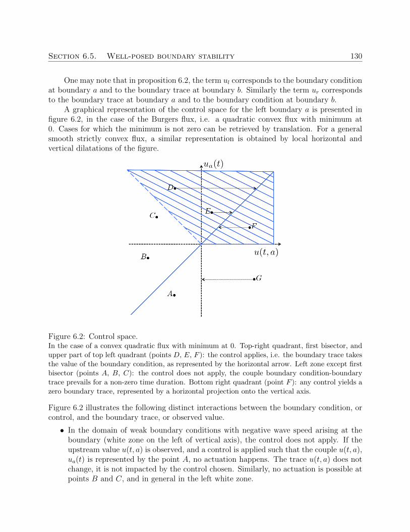
Section 6.5. Well-posed boundary stability 130
One may note that in proposition 6.2, the term ul corresponds to the boundary conditionat boundary a and to the boundary trace at boundary b. Similarly the term ur correspondsto the boundary trace at boundary a and to the boundary condition at boundary b.
A graphical representation of the control space for the left boundary a is presented infigure 6.2, in the case of the Burgers flux, i.e. a quadratic convex flux with minimum at0. Cases for which the minimum is not zero can be retrieved by translation. For a generalsmooth strictly convex flux, a similar representation is obtained by local horizontal andvertical dilatations of the figure.
Figure 6.2: Control space.In the case of a convex quadratic flux with minimum at 0. Top-right quadrant, first bisector, andupper part of top left quadrant (points D, E, F ): the control applies, i.e. the boundary trace takesthe value of the boundary condition, as represented by the horizontal arrow. Left zone except firstbisector (points A, B, C): the control does not apply, the couple boundary condition-boundarytrace prevails for a non-zero time duration. Bottom right quadrant (point F ): any control yields azero boundary trace, represented by a horizontal projection onto the vertical axis.
Figure 6.2 illustrates the following distinct interactions between the boundary condition, orcontrol, and the boundary trace, or observed value.
• In the domain of weak boundary conditions with negative wave speed arising at theboundary (white zone on the left of vertical axis), the control does not apply. If theupstream value u(t, a) is observed, and a control is applied such that the couple u(t, a),ua(t) is represented by the point A, no actuation happens. The trace u(t, a) does notchange, it is not impacted by the control chosen. Similarly, no actuation is possible atpoints B and C, and in general in the left white zone.
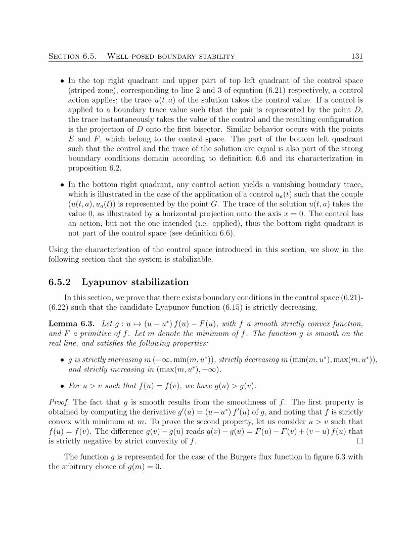
Section 6.5. Well-posed boundary stability 131
• In the top right quadrant and upper part of top left quadrant of the control space(striped zone), corresponding to line 2 and 3 of equation (6.21) respectively, a controlaction applies; the trace u(t, a) of the solution takes the control value. If a control isapplied to a boundary trace value such that the pair is represented by the point D,the trace instantaneously takes the value of the control and the resulting configurationis the projection of D onto the first bisector. Similar behavior occurs with the pointsE and F , which belong to the control space. The part of the bottom left quadrantsuch that the control and the trace of the solution are equal is also part of the strongboundary conditions domain according to definition 6.6 and its characterization inproposition 6.2.
• In the bottom right quadrant, any control action yields a vanishing boundary trace,which is illustrated in the case of the application of a control ua(t) such that the couple(u(t, a), ua(t)) is represented by the point G. The trace of the solution u(t, a) takes thevalue 0, as illustrated by a horizontal projection onto the axis x = 0. The control hasan action, but not the one intended (i.e. applied), thus the bottom right quadrant isnot part of the control space (see definition 6.6).
Using the characterization of the control space introduced in this section, we show in thefollowing section that the system is stabilizable.
6.5.2 Lyapunov stabilization
In this section, we prove that there exists boundary conditions in the control space (6.21)-(6.22) such that the candidate Lyapunov function (6.15) is strictly decreasing.
Lemma 6.3. Let g : u 7→ (u − u∗) f(u) − F (u), with f a smooth strictly convex function,and F a primitive of f . Let m denote the minimum of f . The function g is smooth on thereal line, and satisfies the following properties:
• g is strictly increasing in (−∞,min(m,u∗)), strictly decreasing in (min(m,u∗),max(m,u∗)),and strictly increasing in (max(m,u∗),+∞).
• For u > v such that f(u) = f(v), we have g(u) > g(v).
Proof. The fact that g is smooth results from the smoothness of f . The first property isobtained by computing the derivative g′(u) = (u−u∗) f ′(u) of g, and noting that f is strictlyconvex with minimum at m. To prove the second property, let us consider u > v such thatf(u) = f(v). The difference g(v)− g(u) reads g(v)− g(u) = F (u)−F (v) + (v− u) f(u) thatis strictly negative by strict convexity of f .
The function g is represented for the case of the Burgers flux function in figure 6.3 withthe arbitrary choice of g(m) = 0.
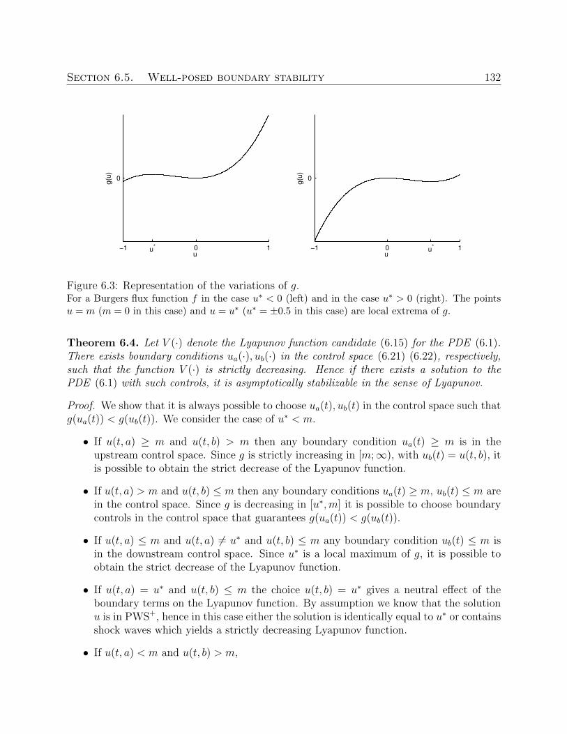
Section 6.5. Well-posed boundary stability 132
−1 u* 0 1
0
u
g(u
)
u
g(u
)
−1 0 u* 1
0
Figure 6.3: Representation of the variations of g.For a Burgers flux function f in the case u∗ < 0 (left) and in the case u∗ > 0 (right). The pointsu = m (m = 0 in this case) and u = u∗ (u∗ = ±0.5 in this case) are local extrema of g.
Theorem 6.4. Let V (·) denote the Lyapunov function candidate (6.15) for the PDE (6.1).There exists boundary conditions ua(·), ub(·) in the control space (6.21) (6.22), respectively,such that the function V (·) is strictly decreasing. Hence if there exists a solution to thePDE (6.1) with such controls, it is asymptotically stabilizable in the sense of Lyapunov.
Proof. We show that it is always possible to choose ua(t), ub(t) in the control space such thatg(ua(t)) < g(ub(t)). We consider the case of u∗ < m.
• If u(t, a) ≥ m and u(t, b) > m then any boundary condition ua(t) ≥ m is in theupstream control space. Since g is strictly increasing in [m;∞), with ub(t) = u(t, b), itis possible to obtain the strict decrease of the Lyapunov function.
• If u(t, a) > m and u(t, b) ≤ m then any boundary conditions ua(t) ≥ m, ub(t) ≤ m arein the control space. Since g is decreasing in [u∗,m] it is possible to choose boundarycontrols in the control space that guarantees g(ua(t)) < g(ub(t)).
• If u(t, a) ≤ m and u(t, a) 6= u∗ and u(t, b) ≤ m any boundary condition ub(t) ≤ m isin the downstream control space. Since u∗ is a local maximum of g, it is possible toobtain the strict decrease of the Lyapunov function.
• If u(t, a) = u∗ and u(t, b) ≤ m the choice u(t, b) = u∗ gives a neutral effect of theboundary terms on the Lyapunov function. By assumption we know that the solutionu is in PWS+, hence in this case either the solution is identically equal to u∗ or containsshock waves which yields a strictly decreasing Lyapunov function.
• If u(t, a) < m and u(t, b) > m,
Section 6.6. Maximizing Lyapunov function decrease rate 133
– If g(u(t, a)) < g(u(t, b)) the choice ua(t) = u(t, a) and ub(t) = u(t, b) in the controlspace leads to the strict decrease of the Lyapunov function.
– If g(u(t, a)) ≥ g(u(t, b)) and u(t, a) 6= u∗, since u∗ is a local maximum of g andaccording to second result of lemma 6.3, it is possible to pick ub(t) ≤ m such thatf(ub) > f(u(t, b)) and g(ub) > g(u(t, a)).
– If g(u(t, a)) ≥ g(u(t, b)) and u(t, a) = u∗, the choice ub(t) = u∗ is in the down-stream control space and yields a neutral effect of the boundary terms. Similarlyto above, by assumption on the regularity of the solution, we have either thesolution identically equal to u∗ or the Lyapunov function strictly decreasing.
The case u∗ > m can be treated similarly. The case u∗ = m can be treated similarly,however involves greater reliance on the internal dynamics. Specifically internal dynamicsare the sole contributor to the decrease of the Lyapunov function in the case 2 and 4 above,and the controller is passive (equal to the boundary trace) in the case 5 above.
Remark 6.5. From the proof of theorem 6.4 it is clear that the stabilizing control is apiecewise continuous function of the boundary trace. Since the solution is piecewise smoothwith a finite number of discontinuities, the boundary condition exhibits no more than a finitenumber of discontinuities. These discontinuities induce rarefaction waves or shock waves,which preserve the piecewise smooth nature of the solution.
In the following section we propose a control design which maximizes the instantaneousdecrease rate of the Lyapunov function.
6.6 Maximizing Lyapunov function decrease rate
In this section, we characterize the values of the control, in the control space, that min-imize the Lyapunov function derivative. Since boundary controls introducing a shock wavecontribute with a negative term to the internal dynamics, we propose to first characterizethe type of wave introduced in specific regions of the control space.
6.6.1 Nature of the waves created by boundary control
The type of wave created at the boundary impacts the value of the derivative of theLyapunov function. In the scalar case, the type of wave arising is defined by the Lax entropycondition (6.8). This allows us to partition the control space according to the type of waveintroduced by the control. Table 6.1 summarizes for the upstream boundary the cases inwhich the boundary control belongs to the control space, with mention of the type of waveintroduced.
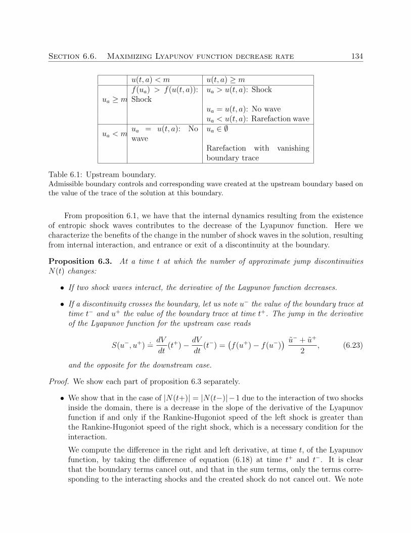
Section 6.6. Maximizing Lyapunov function decrease rate 134
u(t, a) < m u(t, a) ≥ m
ua ≥ mf(ua) > f(u(t, a)):Shock
ua > u(t, a): Shock
ua = u(t, a): No waveua < u(t, a): Rarefaction wave
ua < mua = u(t, a): Nowave
ua ∈ ∅
Rarefaction with vanishingboundary trace
Table 6.1: Upstream boundary.Admissible boundary controls and corresponding wave created at the upstream boundary based onthe value of the trace of the solution at this boundary.
From proposition 6.1, we have that the internal dynamics resulting from the existenceof entropic shock waves contributes to the decrease of the Lyapunov function. Here wecharacterize the benefits of the change in the number of shock waves in the solution, resultingfrom internal interaction, and entrance or exit of a discontinuity at the boundary.
Proposition 6.3. At a time t at which the number of approximate jump discontinuitiesN(t) changes:
• If two shock waves interact, the derivative of the Laypunov function decreases.
• If a discontinuity crosses the boundary, let us note u− the value of the boundary trace attime t− and u+ the value of the boundary trace at time t+. The jump in the derivativeof the Lyapunov function for the upstream case reads
S(u−, u+).=dV
dt(t+)− dV
dt(t−) =
(f(u+)− f(u−)
) u− + u+
2, (6.23)
and the opposite for the downstream case.
Proof. We show each part of proposition 6.3 separately.
• We show that in the case of |N(t+)| = |N(t−)|−1 due to the interaction of two shocksinside the domain, there is a decrease in the slope of the derivative of the Lyapunovfunction if and only if the Rankine-Hugoniot speed of the left shock is greater thanthe Rankine-Hugoniot speed of the right shock, which is a necessary condition for theinteraction.
We compute the difference in the right and left derivative, at time t, of the Lyapunovfunction, by taking the difference of equation (6.18) at time t+ and t−. It is clearthat the boundary terms cancel out, and that in the sum terms, only the terms corre-sponding to the interacting shocks and the created shock do not cancel out. We note
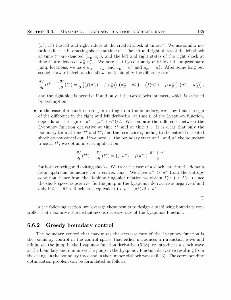
Section 6.6. Maximizing Lyapunov function decrease rate 135
(u+l , u
+r ) the left and right values at the created shock at time t+. We use similar no-
tations for the interacting shocks at time t−. The left and right states of the left shockat time t− are denoted (u−1l, u
−1r), and the left and right states of the right shock at
time t− are denoted (u−2l, u−2r). We note that by continuity outside of the approximate
jump locations, we have u−1r = u−2l, and u−1l = u+l and u−2r = u+
r . After some long butstraightforward algebra, this allows us to simplify the difference to:
dV
dt(t+)− dV
dt(t−) =
1
2
[(f(u−1r)− f(u−1l)
) (u−2l − u
−2r
)+(f(u−2r)− f(u−2l)
) (u−1r − u−1l
)],
and the right side is negative if and only if the two shocks intersect, which is satisfiedby assumption.
• In the case of a shock entering or exiting from the boundary, we show that the signof the difference in the right and left derivative, at time t, of the Lyapunov function,depends on the sign of u∗ − (u− + u+)/2. We compute the difference between theLyapunov function derivative at time t+ and at time t−. It is clear that only theboundary term at time t+ and t−, and the term corresponding to the entered or exitedshock do not cancel out. If we note u− the boundary trace at t− and u+ the boundarytrace at t+, we obtain after simplification:
dV
dt(t+)− dV
dt(t−) =
(f(u+)− f(u−)
) u− + u+
2,
for both entering and exiting shocks. We treat the case of a shock entering the domainfrom upstream boundary for a convex flux. We have u+ > u− from the entropycondition, hence from the Rankine-Hugoniot relation we obtain f(u+) > f(u−) sincethe shock speed is positive. So the jump in the Lyapunov derivative is negative if andonly if u− + u+ < 0, which is equivalent to (u− + u+)/2 < u∗.
In the following section, we leverage these results to design a stabilizing boundary con-troller that maximizes the instantaneous decrease rate of the Lyapunov function.
6.6.2 Greedy boundary control
The boundary control that maximizes the decrease rate of the Lyapunov function isthe boundary control in the control space, that either introduces a rarefaction wave andminimizes the jump in the Lyapunov function derivative (6.18), or introduces a shock waveat the boundary and minimizes the jump in the Lyapunov function derivative resulting fromthe change in the boundary trace and in the number of shock waves (6.23). The correspondingoptimization problem can be formulated as follows.
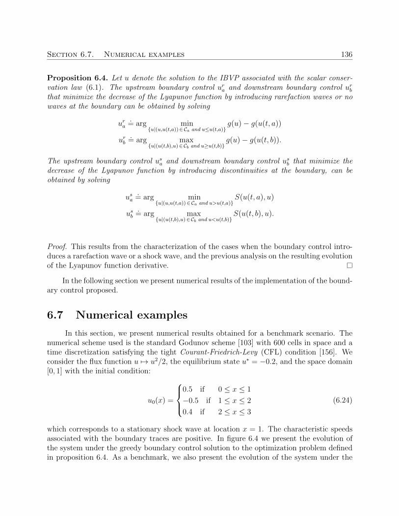
Section 6.7. Numerical examples 136
Proposition 6.4. Let u denote the solution to the IBVP associated with the scalar conser-vation law (6.1). The upstream boundary control ura and downstream boundary control urbthat minimize the decrease of the Lyapunov function by introducing rarefaction waves or nowaves at the boundary can be obtained by solving
ura.= arg min
u|(u,u(t,a))∈Ca and u≤u(t,a)g(u)− g(u(t, a))
urb.= arg max
u|(u(t,b),u)∈Cb and u≥u(t,b)g(u)− g(u(t, b)).
The upstream boundary control usa and downstream boundary control usb that minimize thedecrease of the Lyapunov function by introducing discontinuities at the boundary, can beobtained by solving
usa.= arg min
u|(u,u(t,a))∈Ca and u>u(t,a)S(u(t, a), u)
usb.= arg max
u|(u(t,b),u)∈Cb and u<u(t,b)S(u(t, b), u).
Proof. This results from the characterization of the cases when the boundary control intro-duces a rarefaction wave or a shock wave, and the previous analysis on the resulting evolutionof the Lyapunov function derivative.
In the following section we present numerical results of the implementation of the bound-ary control proposed.
6.7 Numerical examples
In this section, we present numerical results obtained for a benchmark scenario. Thenumerical scheme used is the standard Godunov scheme [103] with 600 cells in space and atime discretization satisfying the tight Courant-Friedrich-Levy (CFL) condition [156]. Weconsider the flux function u 7→ u2/2, the equilibrium state u∗ = −0.2, and the space domain[0, 1] with the initial condition:
u0(x) =
0.5 if 0 ≤ x ≤ 1
−0.5 if 1 ≤ x ≤ 2
0.4 if 2 ≤ x ≤ 3
(6.24)
which corresponds to a stationary shock wave at location x = 1. The characteristic speedsassociated with the boundary traces are positive. In figure 6.4 we present the evolution ofthe system under the greedy boundary control solution to the optimization problem definedin proposition 6.4. As a benchmark, we also present the evolution of the system under the
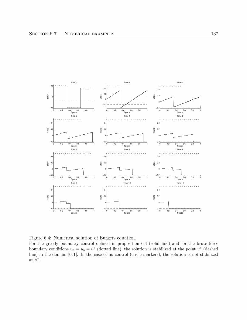
Section 6.7. Numerical examples 137
0 0.2 0.4 0.6 0.8 1
−0.5
0
0.5
Space
Sta
te
Time 0
0 0.2 0.4 0.6 0.8 1
−0.2
0
0.2
0.4
Space
Sta
te
Time 1
0 0.2 0.4 0.6 0.8 1−0.2
0
0.2
0.4
Space
Sta
te
Time 2
0 0.2 0.4 0.6 0.8 1−0.2
0
0.2
0.4
Space
Sta
te
Time 3
0 0.2 0.4 0.6 0.8 1−0.2
0
0.2
0.4
Space
Sta
te
Time 4
0 0.2 0.4 0.6 0.8 1−0.2
0
0.2
0.4
Space
Sta
te
Time 5
0 0.2 0.4 0.6 0.8 1−0.2
0
0.2
0.4
Space
Sta
te
Time 6
0 0.2 0.4 0.6 0.8 1−0.2
0
0.2
0.4
Space
Sta
te
Time 7
0 0.2 0.4 0.6 0.8 1−0.2
0
0.2
0.4
Space
Sta
te
Time 8
0 0.2 0.4 0.6 0.8 1−0.2
0
0.2
0.4
Space
Sta
te
Time 9
0 0.2 0.4 0.6 0.8 1−0.2
0
0.2
0.4
Space
Sta
te
Time 10
0 0.2 0.4 0.6 0.8 1−0.2
0
0.2
0.4
Space
Sta
te
Time 11
Figure 6.4: Numerical solution of Burgers equation.For the greedy boundary control defined in proposition 6.4 (solid line) and for the brute forceboundary conditions ua = ub = u∗ (dotted line), the solution is stabilized at the point u∗ (dashedline) in the domain [0, 1]. In the case of no control (circle markers), the solution is not stabilizedat u∗.
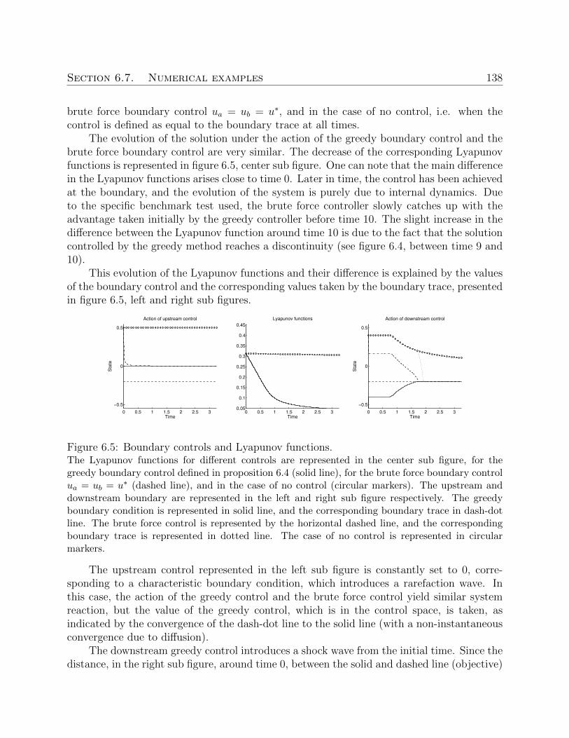
Section 6.7. Numerical examples 138
brute force boundary control ua = ub = u∗, and in the case of no control, i.e. when thecontrol is defined as equal to the boundary trace at all times.
The evolution of the solution under the action of the greedy boundary control and thebrute force boundary control are very similar. The decrease of the corresponding Lyapunovfunctions is represented in figure 6.5, center sub figure. One can note that the main differencein the Lyapunov functions arises close to time 0. Later in time, the control has been achievedat the boundary, and the evolution of the system is purely due to internal dynamics. Dueto the specific benchmark test used, the brute force controller slowly catches up with theadvantage taken initially by the greedy controller before time 10. The slight increase in thedifference between the Lyapunov function around time 10 is due to the fact that the solutioncontrolled by the greedy method reaches a discontinuity (see figure 6.4, between time 9 and10).
This evolution of the Lyapunov functions and their difference is explained by the valuesof the boundary control and the corresponding values taken by the boundary trace, presentedin figure 6.5, left and right sub figures.
0 0.5 1 1.5 2 2.5 30.05
0.1
0.15
0.2
0.25
0.3
0.35
0.4
0.45
Time
Lyapunov functions
0 0.5 1 1.5 2 2.5 3
−0.5
0
0.5
Time
Action of upstream control
Sta
te
0 0.5 1 1.5 2 2.5 3
−0.5
0
0.5
Time
Action of downstream control
Sta
te
Figure 6.5: Boundary controls and Lyapunov functions.The Lyapunov functions for different controls are represented in the center sub figure, for thegreedy boundary control defined in proposition 6.4 (solid line), for the brute force boundary controlua = ub = u∗ (dashed line), and in the case of no control (circular markers). The upstream anddownstream boundary are represented in the left and right sub figure respectively. The greedyboundary condition is represented in solid line, and the corresponding boundary trace in dash-dotline. The brute force control is represented by the horizontal dashed line, and the correspondingboundary trace is represented in dotted line. The case of no control is represented in circularmarkers.
The upstream control represented in the left sub figure is constantly set to 0, corre-sponding to a characteristic boundary condition, which introduces a rarefaction wave. Inthis case, the action of the greedy control and the brute force control yield similar systemreaction, but the value of the greedy control, which is in the control space, is taken, asindicated by the convergence of the dash-dot line to the solid line (with a non-instantaneousconvergence due to diffusion).
The downstream greedy control introduces a shock wave from the initial time. Since thedistance, in the right sub figure, around time 0, between the solid and dashed line (objective)
Section 6.7. Numerical examples 139
is smaller than the distance between the circular marker (boundary trace with no action) andthe dashed line, this clearly contributes to the decrease of the Lyapunov function. However,it is observed that the dash-dot line decreases instantaneously toward the solid line but thenstays stationary at a value different from the solid line. This discrepancy is a consequenceof discretization, and of the fact that the discrepancy prevails in time, which is due the factthat the boundary condition cannot propagate further into the domain, due to the currentvalue of the solution, before time 1.7. Indeed the stationary boundary trace is close to 0.2,and the boundary condition is around −0.4, hence the trace should take the value −0.4.However the value of the solution inside the domain toward the downstream boundary is0.4, hence the action of the control is exactly compensated by the internal dynamics, whichis not observable from the boundary. Hence the control does not have significant action.This is an inherent limitation to boundary control for conservation laws.
Note that while it might seem disappointing that the greedy Lyapunov approach per-forms as well as the brute force approach, its superiority is twofold:
• It is proven to stabilize the system, whereas the brute force approach can only bechecked post-facto, assuming it works.
• The controller does effectively apply. Conversely the brute force approach is ineffectivein the sense that the prescribed value of the controller does not necessarily apply.
140
Chapter 7
Contributions and open problems
This dissertation work has been pursued in the context of the Mobile Millennium projectand the revolution in traffic monitoring systems owing to the explosion of mobile devices inthe world. The resulting paradigm changes in the field of traffic engineering motivated asignificant proportion of the research endeavors considered in this work.
The emergence of mobile sensing and the mass of associated streaming velocity measure-ments motivated research efforts on novel traffic models and estimation algorithms. Investi-gations on the equivalence of velocity-based conservation laws and density-based conservationlaws, as well as the theoretical research on higher-order PDE models, led to successful im-plementations at a large scale (Northern California road network) in the real-time MobileMillennium system.
However, the issues of data quality and model error, considerably emphasized by crowd-sourcing in an online real-time environment, called for the development of advanced dataassimilation techniques and the proper understanding of their underlying uncertainty struc-ture given the properties of the mathematical models used. Precise knowledge of the accu-racy of the estimates provided in real-time is a critical factor to the applicability of a trafficmonitoring system, especially in a large-scale system in which so-called ground-truth is notdirectly available.
The control problems investigated during this dissertation, at a macroscopic level for flowcontrol in the previous chapter, as well as the stochastic on-time arrival routing problem [191,35], which was implemented and applied in an operational setting to traffic estimates based onthe modeling and estimation work described in this dissertation and in [227] in particular,delineate the state of the art in the mathematics of traffic monitoring, and the emergingdirections for the future science of intelligent large-scale infrastructure.
141
The contribution of this thesis and the natural extensions to this work are as follows.
2×2 phase transition model of traffic flow. Chapter 2 presented an extension to theoriginal phase transition model presented by Colombo. The model proposed accounts for thevariability of traffic state due to heterogeneous driving behaviors, and different traffic pat-terns at different locations. The Cauchy problem associated with the system of hyperbolicconservation laws was shown to be well-posed in L1 ∩ BV . A Riemann solver was con-structed, and a numerical discretization scheme derived from the classical Godunov schemeimplemented.
Extensions to this work include the proper formulation of the junction problem formodeling traffic flow at road crossings using a 2×2 traffic model. It is known that congestionis created at junctions and at the location of sudden driving maneuvers. The contribution ofthis work has been to provide mathematical tools to model non standard individual trafficbehaviors. The problem of junction modeling has been solved for scalar traffic models butfew results exist for non-scalar network models of traffic flow.
A theoretical problem of significant practical importance is the problem of mixed dis-tributed and boundary control from eulerian and lagrangian actuators in the presence oflimited information. Mathematical resolution of this problem would allow identifying a setof optimal ramp metering and probe-enforced variable speed limits for congestion mitigation.Unfortunately, standard approaches lead to ill-posed problems and non-realistic results. Theuse of a non-scalar model that properly accounts for macroscopic and microscopic trafficphenomena would allow great progress in this direction.
Estimation methods for non-scalar traffic models. Chapter 3 presented an as-sessment of the performance of the 2 × 2 phase transition model for time space diagramreconstruction, based on initial and boundary data extracted from high resolution camera-based experimental vehicle trajectories. The results were shown in a forward-simulationsetting, in which perfect joint measurements from coincidental loop detectors and probevehicles are collected. This ideal scenario allowed the identification of the propagation offorward-moving discontinuity in congested traffic flow, which had not been surely observedpreviously in the literature, and the assessment of the greater robustness of the 2× 2 modelto calibration error.
Extensions to this work include the use of a proper estimation framework in order toassess the impact of observation error and model error on the accuracy of the estimates.The problem of data fusion from loop detectors and probe vehicles is also a very importantpractical question.
Finally, the use of such macroscopic models able to account for heterogeneous drivingbehavior would be of great interest for the design of stochastic routing algorithms [35, 191],which require the knowledge of the cause of the traffic state estimate distribution variance;from a routing perspective, a large link travel-time variance caused by driver heterogeneity isvery different from a large link travel-time variance due to algorithmic and data limitationscorresponding to numerical uncertainty.
142
Adaptive estimation algorithms. In Chapter 5, a model-based analysis of the con-sequence of nonlinearity and non-differentiability on estimation error, and specifically on thestructure of the uncertainty propagated by suboptimal filtering algorithms was presented. Itwas shown that the emergence of discontinuities in the solution to scalar hyperbolic conser-vation laws causes the emergence of mixture uncertainty distribution on the traffic state, andthe robustness of stochastic filters to this uncertainty structure was assessed numerically.
This work paves the ground for smart adaptive estimation methods and filtering al-gorithms. Advanced estimation methods currently applied to traffic monitoring are derivedfrom the theory of linear dynamical systems. The design of real-time online provably optimalsequential estimation algorithms for specific non-linear conservation law models is still anopen problem.
A second extension to this work relates to the notion of data quality. With the increasedvolume of crowd-sourced data used for large scale civil infrastructure monitoring, the abilityto track down the nature of errors and the location of uncertainty is a critical feature ofestimation algorithms, in particular for safety-sensitive cyber-physical systems. State-of-theart estimation methods provide online estimates which are derived from prior knowledgeof model and observation errors. However, estimation algorithms are currently not boundto online quality criteria, which could be designed using the methods introduced in this work.
Boundary stabilization of weak entropy solutions. Chapter 6 proposed a bound-ary control design that guarantees the greedy decrease of a Lyapunov function candidate.This result solves a problem that has been approached in the literature with many differenttools. In particular, our method accounts for the proper treatment of weak boundary con-ditions, the correct structure of emerging entropic shock waves in the solution to the partialdifferential equation, and allows the consideration of physical constraints on the control, inparticular its total variation.
The approach chosen in this work is based on the assumption of the piecewise regularityof the solution, which is a standard assumption in the conservation laws community. Adifferent approach can be based on general wave-front tracking approximations, which exhibitby nature a piecewise-constant property and approximate arbitrarily closely a BV solution.Another approach can be considered from the perspective of Hamilton-Jacobi equation, forwhich the gradient of the Barron-Jensen-Frankowska solutions has recently been shown tocoincide with the classical weak entropy solutions of the associated conservation law.
Extensions to this work include the development of similar techniques for non-scalarmodels of traffic, in which the more complex structure of the Riemann invariants allowsmore complex controls. A problem of great interest for practical applications is the problemof well-posed distributed stabilization of traffic flow on corridors.
143
Bibliography
[1] K. Ahmed, M. Ben-Akiva, H. Koutsopoulos, and R. Mishalani. Models offreeway lane changing and gap acceptance behavior. In Proceedings of the 13th In-ternational Symposium on Transportation and Traffic Theory, Lyon, France, pages501–515, 1996. 47
[2] A. Allstrom, J. Archer, A. Bayen, S. Blandin, J. Butler, D. Gundlegard,H. Koutsopoulos, J. Lundgren, M. Rahmani, and O.-P. Tossavainen. MobileMillennium Stockholm. In 2nd International Conference on Models and Technologiesfor Intelligent Transportation Systems, Leuven, Belgium June 2011. 2, 14
[3] D. Amadori. Initial-boundary value problems for nonlinear systems of conservationlaws. NoDEA: Nonlinear Differential Equations and Applications, 4(1):1–42, 1997.121, 123
[4] D. Amadori and R. Colombo. Continuous dependence for 2 × 2 conservation lawswith boundary. Journal of Differential Equations, 138(2):229–266, 1997. 123
[5] D. Amadori and R. Colombo. Viscosity solutions and standard Riemann semigroupfor conservation laws with boundary. Rendiconti del Seminario Matematico della Uni-versita di Padova, 99:219–245, 1998. 123
[6] S. Amin, F. Hante, and A. Bayen. On stability of switched linear hyperbolic con-servation laws with reflecting boundaries. Hybrid System: Computation and Control,Lecture Notes in Computer Science, 4981:602–605, 2008, doi:10.1007/978-3-540-78929-144. 117
[7] S. Amin, F. Hante, and A. Bayen. Exponential stability of switched linear hyperbolicinitial-boundary value problems. IEEE Transactions on Automatic Control, 57(2):291–301, 2012, doi:10.1109/TAC.2011.2158171. 117
[8] F. Ancona and P. Goatin. Uniqueness and stability of L∞ solutions for Templeclass systems with boundary and properties of the attainable sets. SIAM Journal onMathematical Analysis, 34(1):28–63, 2002. 117
[9] B. Anderson and J. Moore. Optimal filtering. Prentice Hall, Upper Saddle River,NJ, 1979. 12
[10] J. Anderson. An ensemble adjustment Kalman filter for data assimilation. Monthlyweather review, 129(12):2884–2903, 2001. 92
[11] C. Andrieu, N. De Freitas, A. Doucet, and M. Jordan. An introduction toMCMC for machine learning. Journal of Machine learning, 50(1):5–43, 2003. 92
BIBLIOGRAPHY 144
[12] J.-P. Aubin, A. Bayen, and P. Saint-Pierre. Dirichlet problems for some Hamilton-Jacobi equations with inequality constraints. SIAM Journal on Control and Optimiza-tion, 47(5):2348–2380, 2008, doi:10.1137/060659569. 117
[13] A. Aw and M. Rascle. Resurrection of “second order” models of traffic flow. SIAMJournal on Applied Mathematics, 60(3):916–938, 2000. 5, 9, 50
[14] J. Barcelo, J. Casas, J. Ferrer, and D. Garcia. Modelling advanced transporttelematic applications with microscopic simulators: The case with AIMSUN2. InProceedings of the 10th European Simulation Symposium, Nottingham, UK, pages 362–367, 1998. 48
[15] C. Bardos, A.-Y. Leroux, and J.-C. Nedelec. First order quasilinear equationswith boundary conditions. Communications in partial differential equations, 4(9):1017–1034, 1979. 4, 121, 123
[16] C. Bardos and O. Pironneau. Derivatives and control in the presence of shocks.Computational Fluid Dynamics Journal, 11(4):383–391, 2003. 118
[17] Y. Bar-Shalom, X. Li, T. Kirubarajan, and J. Wiley. Estimation with applica-tions to tracking and navigation. John Wiley and Sons, New York, NY, 2001. 10
[18] G. Bastin, B. Haut, J.-M. Coron, and B. d Andrea-Novel. Lyapunov stabilityanalysis of networks of scalar conservation laws. Networks and Heterogeneous Media,2(4):751–759, 2007. 117
[19] A. Bayen, J. Butler, and A. Patire. Mobile Millennium final report. Technicalreport, California Center for Innovative Transportation, Institute of TransportationStudies, University of California, Berkeley, Research Report, UCB-ITS-CWP-2011-6,2011. 2, 48
[20] A. Bayen, R. Raffard, and C. Tomlin. Adjoint-based control of a new euleriannetwork model of air traffic flow. IEEE Transactions on Control Systems Technology,14(5):804–818, 2006. 118
[21] M. Ben-Akiva, M. Bierlaire, H. Koutsopoulos, and R. Mishalani. Real-timesimulation of traffic demand-supply interactions within DynaMIT. Transportation andnetwork analysis: current trends: miscellanea in honor of Michael Florian, 63:19–36,2002. 48
[22] S. Bianchini. On the shift differentiability of the flow generated by a hyperbolicsystem of conservation laws. Discrete and Continuous Dynamical Systems, 6(2):329–350, 2000. 118
[23] S. Blandin, J. Argote, D. Work, and A. Bayen. A phase transition model ofnon stationary traffic flow: definition, properties and solution method. Submitted toTransportation Research Part B. 13
[24] S. Blandin, G. Bretti, A. Cutolo, and B. Piccoli. Numerical simulations of trafficdata via fluid dynamic approach. Applied Mathematics and Computation, 210(2):441–454, 2009, doi:10.1016/j.amc.2009.01.057. 14, 19
[25] S. Blandin, A. Couque, A. Bayen, and D. Work. On sequential data assimila-tion for scalar macroscopic traffic flow models. In Review for Physica D: NonlinearPhenomena, 2011., 2012. 13, 50
BIBLIOGRAPHY 145
[26] S. Blandin, L. El Ghaoui, and A. Bayen. Kernel regression for travel-time estimationvia convex optimization. In IEEE Conference on Decision and Control, Shanghai,China, December 2009. 14
[27] S. Blandin, X. Litrico, and A. Bayen. Boundary stabilization of the unviscidBurgers equation using a Lyapunov method. In Proceedings of the 49th IEEE Con-ference on Decision and Controls, 2010 Atlanta, Georgia, pages 1705–1712, 2010,doi:10.1109/CDC.2010.5717716. 13, 129
[28] S. Blandin, X. Litrico, B. Piccoli, and A. Bayen. Boundary stabilization of thetransport equation using a Lyapunov method. In preparation for the IEEE Transac-tions on Automatic Control. 13
[29] S. Blandin, A. Salam, and A. Bayen. Individual speed variance in traffic flow: anal-ysis of bay area radar measurements. In Transportation Research Board 91st AnnualMeeting, Washington, D.C., Jan. 22–26, 2012. 14
[30] S. Blandin, D. Work, P. Goatin, B. Piccoli, and A. Bayen. A class of perturbedcell transmission models to account for traffic variability. In 89th Transportation Re-search Board Annual Meeting, Washington D.C., January 10-14, 2010. 13, 51
[31] S. Blandin, D. Work, P. Goatin, B. Piccoli, and A. Bayen. A general phase tran-sition model for vehicular traffic. SIAM Journal on Applied Mathematics., 71(1):107–121, 2011. 9, 13, 63, 95
[32] S. Blandin, D. Work, P. Goatin, B. Piccoli, and A. Bayen. A general phasetransition model for vehicular traffic. In IFAC workshop on Control of DistributedParameter Systems, France, 2009. 13
[33] M. Bocquet, C. Pires, and L. Wu. Beyond Gaussian statistical modeling in geo-physical data assimilation. Monthly Weather Review, 138:2997–3023, 2010. 94
[34] R. Boel and L. Mihaylova. A compositional stochastic model for real time freewaytraffic simulation. Transportation Research Part B, 40(4):319–334, 2006. 92
[35] P. Borokhov, S. Blandin, S. Samaranayake, O. Goldschmidt, and A. Bayen.An adaptive routing system for location-aware mobile devices on the road network.In IEEE Intelligent Transportation Systems Conference, Washington, D.C., October2011, 2011, doi:10.1109/ITSC.2011.6083021. 14, 140, 141
[36] F. Bouttier and P. Courtier. Data assimilation concepts and methods. Trainingcourse notes of the European Centre for Medium-Range Weather Forecasts, 1999,Reading, UK, 1999. 9, 85
[37] F. Brauer and J. Nohel. The qualitative theory of ordinary differential equations:an introduction. Dover, Mineola, NY, 1989. 47
[38] A. Bressan. The unique limit of the Glimm scheme. Archive for Rational Mechanicsand Analysis, 130(3):205–230, 1995. 123
[39] A. Bressan. Hyperbolic systems of conservation laws: the one-dimensional Cauchyproblem. Oxford University Press, Oxford, UK, 2000. 8, 16, 24, 25, 44, 70, 94, 119
[40] A. Bressan, G. Crasta, and B. Piccoli. Well-posedness of the Cauchy problem forn× n systems of conservation laws. American Mathematical Society, Providence, RI,2000. 3, 4, 125
BIBLIOGRAPHY 146
[41] A. Bressan and G. Guerra. Shift-differentiabilitiy of the flow generated by a con-servation law. Discrete and Continuous Dynamical Systems, 3:35–58, 1997. 118
[42] G. Burgers, P. van Leeuwen, and G. Evensen. Analysis scheme in the ensembleKalman filter. Monthly Weather Review, 126(6):1719–1724, 1998. 91
[43] J. Burns and S. Kang. A control problem for Burgers equation with bounded in-put/output. Nonlinear Dynamics, 2(4):235–262, 1991. 117
[44] C. Byrnes, D. Gilliam, and V. Shubov. On the global dynamics of a controlledviscous Burgers equation. Journal of Dynamical and Control Systems, 4(4):457–519,1998. 117
[45] G. Cameron and G. Duncan. PARAMICS—Parallel microscopic simulation of roadtraffic. The Journal of Supercomputing, 10(1):25–53, 1996. 47
[46] M. Cassidy. Bivariate relations in nearly stationary highway traffic. TransportationResearch Part B, 32(1):49–59, 1998. 49
[47] M. Cassidy and B. Coifman. Relation among average speed, flow, and density andanalogous relation between density and occupancy. Transportation Research Record:Journal of the Transportation Research Board, 1591:1–6, 1997. 49
[48] M. Cassidy and J Windover. Methodology for assessing dynamics of freeway trafficflow. Transportation Research Record, 1484:73–79, 1995. 4
[49] C. Chalons and P. Goatin. Godunov scheme and sampling technique for computingphase transitions in traffic flow modeling. Interfaces and Free Boundaries, 10(2):195–219, 2008. 27, 28, 63
[50] J. Chandrasekar, A. Ridley, and D. Bernstein. A comparison of the extendedand unscented Kalman filters for discrete-time systems with nondifferentiable dynam-ics. In American Control Conference (ACC), 2007, pages 4431–4436, 2007. 94
[51] R. Chen and J. Liu. Mixture Kalman filters. Journal of the Royal Statistical Society:Series B (Statistical Methodology), 62(3):493–508, 2000. 12, 86
[52] N. Chiabaut, C. Buisson, and L. Leclercq. Fundamental diagram estimationthrough passing rate measurements in congestion. IEEE Transactions on IntelligentTransportation Systems, 10(2):355–359, 2009. 61
[53] N. Chiabaut, L. Leclercq, and C. Buisson. From heterogeneous drivers to macro-scopic patterns in congestion. Transportation Research Part B, 44(2):299–308, 2010.50
[54] D. Chickering and C. Meek. Finding optimal Bayesian networks. In Proceedingsof the Eighteenth Annual Conference on Uncertainty in Artificial Intelligence, pages94–102, San Francisco, CA, 2002. Morgan Kaufmann. 73, 75, 76
[55] A. Chorin and X. Tu. Implicit sampling for particle filters. Proceedings of theNational Academy of Sciences, 106(41):17249–17254, 2009. 93
[56] A. Chow, V. Dadok, G. Dervisoglu, G. Gomes, R. Horowitz, A. Kurzhanski,J. Kwon, and X. Lu. Topl: Tools for operational planning of transportation networks.In Proceedings of the 2008 Dynamic Systems and Control Conference, Ann Arbor,Michigan, pages 20–22, 2008. 48
[57] D. Chowdhury, L. Santen, and A. Schadschneider. Statistical physics of ve-
BIBLIOGRAPHY 147
hicular traffic and some related systems. Physics Reports, 329(4-6):199–329, 2000.48
[58] C. Claudel and A. Bayen. Lax-Hopf Based Incorporation of Internal BoundaryConditions Into Hamilton–Jacobi Equation. Part I: Theory. IEEE Transactions onAutomatic Control, 55(5):1142–1157, 2010, doi:10.1109/TAC.2010.2041976. 8
[59] C. Claudel and A. Bayen. Lax–Hopf Based Incorporation of Internal Boundary Con-ditions Into Hamilton-Jacobi Equation. Part II: Computational Methods. IEEE Trans-actions on Automatic Control, 55(5):1158–1174, 2010, doi:10.1109/TAC.2010.2045439.8
[60] G. Coclite, M. Garavello, and B. Piccoli. Traffic flow on a road network. SIAMJournal on Mathematical Analysis, 36(6):1862–1886, 2005. 6
[61] R. Colombo. On a 2 × 2 hyperbolic traffic flow model. Mathematical and ComputerModelling, 35(5-6):683–688, 2002. 9, 16, 17, 18
[62] R. Colombo. Hyperbolic phase transitions in traffic flow. SIAM Journal on AppliedMathematics, 63(2):708–721, 2003. 16, 17, 19, 21, 24, 25, 29, 31, 35
[63] R. Colombo, P. Goatin, and F. Priuli. Global well-posedness of traffic flow modelswith phase transitions. Nonlinear Analysis, 66(11):2413–2426, 2007. 16, 25, 42
[64] J.-M. Coron, B. d’Andrea-Novel, and G. Bastin. A strict Lyapunov function forboundary control of hyperbolic systems of conservation laws. IEEE Transactions onAutomatic Control, 52(1):2–11, 2007. 117
[65] P. Courtier, E. Andersson, W. Heckley, D. Vasiljevic, M. Hamrud,A. Hollingsworth, F. Rabier, M. Fisher, and J. Pailleux. The ECMWF im-plementation of three-dimensional variational assimilation (3D-Var). I: Formulation.Quarterly Journal of the Royal Meteorological Society, 124(550):1783–1807, 1998. 85
[66] P. Courtier, J. Thepaut, and A. Hollingsworth. A strategy for operationalimplementation of 4D-Var, using an incremental approach. Quarterly Journal of theRoyal Meteorological Society, 120(519):1367–1387, 1994. 85
[67] M. Cremer and M. Papageorgiou. Parameter identification for a traffic flow model.Automatica, 17(6):837–843, 1981. 61
[68] N. Cristianini and J. Shawe-Taylor. An Introduction to Support Vector Machines.Cambridge University Press, Cambridge, UK, 2000. 79
[69] M. Cunha and F. Dorini. Statistical moments of the solution of the random Burgers-Riemann problem. Mathematics and Computers in Simulation, 79(5):1440–1451, 2009.95
[70] C. Dafermos. Hyperbolic conservation laws in continuum physics. Springer-VerlagBerlin, Germany, 2010. 120
[71] C. Daganzo. The cell transmission model: a dynamic representation of highwaytraffic consistent with the hydrodynamic theory. Transportation Research Part B,28(4):269–287, 1994. 4, 8, 49, 73, 86
[72] C. Daganzo. The cell transmission model, part II: Network traffic. TransportationResearch Part B: Methodological, 29(2):79–93, 1995. 4, 5, 6, 8, 86
[73] C. Daganzo. Requiem for second-order fluid approximations of traffic flow. Trans-
BIBLIOGRAPHY 148
portation Research Part B, 29(4):277–286, 1995. 5, 49, 50[74] C. Daganzo, M. Cassidy, and R. Bertini. Possible explanations of phase transitions
in highway traffic. Transportation Research Part A, 33(5):365–379, 1999. 4, 51[75] J. De Halleux, C. Prieur, J.M. Coron, B. d’Andrea-Novel, and G. Bastin.
Boundary feedback control in networks of open channels. Automatica, 39(8):1365–1376,2003. 117
[76] J.M. Del Castillo and F.G. Benitez. On the functional form of the speed-density relationship Part II: empirical investigation. Transportation Research PartB, 29(5):391–406, 1995. 49
[77] J.M. Del Castillo and F.G. Benitez. On the functional form of the speed-densityrelationship I: General theory. Transportation Research Part B, 29(5):373–389, 1995.20
[78] J.M. Del Castillo, P. Pintado, and F.G. Benitez. The reaction time of driversand the stability of traffic flow. Transportation Research Part B, 28(1):35–60, 1994. 5,49, 50
[79] M. Demetriou and I. Hussein. Estimation of spatially distributed processes usingmobile spatially distributed sensor network. SIAM Journal on Control and Optimiza-tion, 48(1):266–291, 2009. 128
[80] R. Dobbs, S. Smit, J. Remes, J. Manyika, C. Roxburgh, and A. Restrepo.Urban world : Mapping the economic power of cities. Technical Report March, McKinsey Global Institute, 2011. 1
[81] V. Dos Santos, G. Bastin, J.-M. Coron, and B. d’Andrea-Novel. Boundarycontrol with integral action for hyperbolic systems of conservation laws: Stability andexperiments. Automatica, 44(5):1310–1318, 2008. 117
[82] F. Dubois and P. LeFloch. Boundary conditions for nonlinear hyperbolic systemsof conservation laws. Journal of Differential Equations, 71(1):93–122, 1988. 121
[83] R. Durrett. Essentials of stochastic processes. Springer, New York, NY, 1999. 73[84] L. Edie. Discussion of traffic stream measurements and definitions. In Proceedings of
the 2nd International Symposium on the Theory of Traffic Flow, London, UK, pages139–154, 1963. 60
[85] L. Edie, R. Foote, R. Herman, and R. Rothery. Analysis of single lane trafficflow. Traffic Engineering, 33(4):21–27, 1963. 49
[86] B. Efron and G. Gong. A leisurely look at the bootstrap, the jackknife, and cross-validation. American Statistician, pages 36–48, 1983. 81
[87] N. El-Farra and P. Christofides. Coordinating feedback and switching for controlof spatially distributed processes. Computers and chemical engineering, 28(1-2):111–128, 2004. 128
[88] H. Engl, K. Kunisch, and A. Neubauer. Convergence rates for Tikhonov regular-ization of nonlinear ill-posed problems. Inverse Problems, 5(4):523–540, 1989. 79
[89] L. Evans. Partial differential equations. American Mathematical Society, Providence,RI, 1998. 3, 87, 95, 120
[90] G. Evensen. Using the extended Kalman filter with a multilayer quasi-geostrophic
BIBLIOGRAPHY 149
ocean model. Journal of Geophysical Research, 97(C11):17905–17924, 1992. 89[91] G. Evensen. Inverse methods and data assimilation in nonlinear ocean models. Phys-
ica D: Nonlinear Phenomena, 77(1-3):108–129, 1994. 85[92] G. Evensen. Sequential data assimilation with a nonlinear quasi-geostrophic model
using Monte Carlo methods to forecast error statistics. Journal of Geophysical Re-search, 99:10143–10162, 1994. 91
[93] G. Evensen. The ensemble Kalman filter: Theoretical formulation and practicalimplementation. Ocean dynamics, 53(4):343–367, 2003. 12, 86, 91
[94] M. Fellendorf. VISSIM: A microscopic simulation tool to evaluate actuated signalcontrol including bus priority. In 64th Institute of Transportation Engineers AnnualMeeting, Dallas, TX, 1994. 47
[95] M. Fliess, J. Levine, P. Martin, and P. Rouchon. Flatness and defect of non-linear systems: introductory theory and examples. International journal of control,61(6):1327–1362, 1995. 117
[96] H. Frankowska. On LeFloch solutions to initial-boundary value problem for scalarconservation laws. Journal of Hyperbolic Differential Equations, 7(3):1–41, 2010. 123
[97] M. Garavello and B. Piccoli. Traffic flow on networks. American Institute ofMathematical Sciences, Springfield, MO, 2006. 6, 17, 48, 95, 123
[98] M. Garavello and B. Piccoli. On fluido-dynamic models for urban traffic. Networkand Heterogeneous Media, 4(1):107–126, 2009. 16
[99] D. Gazis, R. Herman, and R. Potts. Car-following theory of steady-state trafficflow. Operations Research, 7(4):499–505, 1959. 48
[100] D. Gazis and C. Knapp. On-line estimation of traffic densities from time-series offlow and speed data. Transportation Science, 5(3):283–301, 1971. 86
[101] J. Glimm. Solutions in the large for nonlinear hyperbolic systems of equations. Com-munication on pure and applied mathematics, 18:697–715, 1965. 3, 4
[102] P. Goatin. The Aw-Rascle vehicular traffic flow model with phase transitions. Math-ematical and Computer Modelling, 44(3-4):287–303, 2006. 16
[103] S. Godunov. A difference method for numerical calculation of discontinuous solutionsof the equations of hydrodynamics. Matematicheskii Sbornik, 89(3):271–306, 1959. 4,7, 70, 87, 136
[104] G. Gomes and R. Horowitz. Optimal freeway ramp metering using the asymmet-ric cell transmission model. Transportation Research Part C: Emerging Technologies,14(4):244–262, 2006. 118
[105] N. Gordon, D. Salmond, and A. Smith. Novel approach to nonlinear/non-GaussianBayesian state estimation. In Radar and Signal Processing, IEE Proceedings F, volume140, pages 107–113. IET, 1993. 86, 92
[106] H. Greenberg. An analysis of traffic flow. Operations Research, 7(1):79–85, 1959. 4,6, 49
[107] B. Greenshields. A study of traffic capacity. Proceedings of the Highway ResearchBoard, 14(1):448–477, 1935. 4, 5, 18, 49
[108] M. Gugat and G. Leugering. Global boundary controllability of the saint-venant
BIBLIOGRAPHY 150
system for sloped canals with friction. In Annales de l’Institut Henri Poincare, vol-ume 26, pages 257–270. Elsevier, 2009. 117
[109] W. Hastings. Monte-Carlo sampling methods using Markov chains and their appli-cations. Biometrika, 57(1), 1970. 92
[110] D. Haughton. On the choice of a model to fit data from an exponential family. TheAnnals of Statistics, 16(1):342–355, 1988. 74
[111] A. Hegyi, D. Girimonte, R. Babuska, and B. De Schutter. A comparison offilter configurations for freeway traffic state estimation. In Intelligent TransportationSystems Conference, 2006, ITSC 2006., pages 1029–1034, Toronto, CA, 2006. 90, 94
[112] D. Helbing. Improved fluid-dynamic model for vehicular traffic. Physical Review E,51(4):3164–3169, 1995. 9, 50
[113] D. Helbing. Traffic and related self-driven many-particle systems. Reviews of modernphysics, 73(4):1067–1141, 2001. 48
[114] J.-C. Herrera and A. Bayen. Incorporation of Lagrangian measurements in free-way traffic state estimation. Transportation research Part B, 44(4):460–481, 2010,doi:10.1016/j.trb.2009.10.005. 86
[115] T. Hey, S. Tansley, and K. Tolle, editors. The Fourth Paradigm: Data-IntensiveScientific Discovery. Microsoft Research, Redmond, WA, 2009. 2
[116] H. Holden and N. Risebro. A mathematical model of traffic flow on a network ofunidirectional roads. SIAM Journal on Mathematical Analysis, 26(4):999–1017, 1995.6
[117] H. Holden and N. Risebro. Front tracking for hyperbolic conservation laws. Springer-Verlag, New-York, NY, 2002. 16
[118] S. Hoogendorn and P. Bovy. State-of-the-art of vehicular traffic flow modelling.Proceedings of the Institution of Mechanical Engineers, Part I: Journal of Systems andControl Engineering, Special Issue on Road Traffic Modelling and Control, 215:283–303, 2001. 48, 49, 50
[119] C. Huang, Y. Fallah, R. Sengupta, and H. Krishnan. Adaptive intervehiclecommunication control for cooperative safety systems. IEEE Network, 24(1):6–13,2010. 93
[120] J. Huttunen and J. Kaipio. Approximation error analysis in nonlinear state estima-tion with an application to state-space identification. Inverse Problems, 23:2141–2157,2007. 104
[121] J. Huttunen and J. Kaipio. Approximation errors in nonstationary inverse problems.Inverse problems and imaging, 1(1):77–93, 2007. 104
[122] D. Jacquet. Modelisation macroscopique du traffic et controle des lois de conservationnon lineaires associees. PhD thesis, Institut National Polytechnique de Grenoble,Grenoble, France, 2006. 117
[123] D. Jacquet, M. Krstic, and C. Canudas de Wit. Optimal control of scalarone-dimensional conservation laws. In 25th American Control Conference, 2006 Min-neapolis, MN, USA, pages 5213–5218, 2006. 117
[124] A. Jazwinski. Stochastic processes and filtering theory. Academic Press, New York,
BIBLIOGRAPHY 151
NY, 1970. 10[125] F. Jensen and T. Nielsen. Bayesian networks and decision graphs. Springer, New-
York, NY, USA, 2007. 70, 73[126] Z. Jia, C. Chen, B. Coifman, and P. Varaiya. The PeMS algorithms for accu-
rate, real-time estimates of g-factors and speeds from single-loop detectors. In IEEEProceedings of Intelligent Transport Systems, pages 536–541, 2001. 4
[127] W. Jin. A kinematic wave theory of lane-changing traffic flow. Transportation ResearchPart B, 44(8-9):1001–1021, 2010. 50
[128] M. Jordan. Learning in graphical models. MIT Press Cambridge, MA, USA, 1999.70, 71, 72, 73
[129] S. Julier and J. Uhlmann. A new extension of the Kalman filter to nonlinearsystems. In Proceedings of AeroSense: SPIE 11th Annual International Symposium onAerospace/Defense Sensing, Simulation and Controls., Orlando, FL, 1997. 12, 86, 89
[130] S. Julier, J. Uhlmann, and H. Durrant-Whyte. A new method for the nonlineartransformation of means and covariances in filters and estimators. IEEE Transactionson Automatic Control, 45(3):477–482, 2000. 89
[131] J. Kaipio and E. Somersalo. Statistical and computational inverse problems.Springer, New-York, NY, 2005. 9, 11, 70, 85, 101
[132] R. Kalman. A new approach to linear filtering and prediction problems. Journal ofbasic Engineering, 82(1):35–45, 1960. 10, 11, 85
[133] C. Kang and J. Tian. Markov properties for linear causal models with correlatederrors. The Journal of Machine Learning Research, 10:41–70, 2009. 72
[134] B. Kerner. Experimental features of self-organization in traffic flow. Physical ReviewLetters, 81(17):3797–3800, 1998. 16, 50
[135] B. Kerner. Phase transitions in traffic flow. Traffic and granular flow, pages 253–283,2000. 16, 20
[136] B. Kerner and H. Rehborn. Experimental properties of complexity in traffic flow.Physical Review E, 53(5):4275–4278, 1996. 50
[137] B. Kerner and H. Rehborn. Experimental properties of phase transitions in trafficflow. Physical Review Letters, 79(20):4030–4033, 1997. 50
[138] T. Kobayashi. Adaptive regulator design of a viscous Burgers system by boundarycontrol. IMA Journal of Mathematical Control and Information, 18(3):427, 2001. 117
[139] M. Krstic. On global stabilization of Burgers equation by boundary control. Systemsand Control Letters, 37(3):123–141, 1999. 117, 126
[140] M. Krstic and A. Smyshlyaev. Boundary control of PDEs: A Course on Backstep-ping Designs. Society for Industrial and Applied Mathematics Philadelphia, PA, 2008.126
[141] S. Kruzhkov. First order quasilinear equations in several independent variables.Mathematics of the USSR-Sbornik, 10(2):217–243, 1970. 3, 4, 120, 123
[142] G. Lanckriet, N. Cristianini, P. Bartlett, L. El Ghaoui, and M. Jordan.Learning the kernel matrix with semidefinite programming. Journal of Machine Learn-ing Research, 5:27–72, 2004. 81
BIBLIOGRAPHY 152
[143] J. Laval. Linking synchronized flow and kinematic waves. In Proceedings of Trafficand Granular Flow’05, Berlin, Germany, pages 521–526, 2005. 50
[144] J. Laval. Hysteresis in traffic flow revisited: An improved measurement method.Transportation Research Part B, 45(2):385–391, 2011. 56, 58
[145] J. Laval and C. Daganzo. Lane-changing in traffic streams. Transportation ResearchPart B, 40(3):251–264, 2006. 50
[146] J. Laval and L. Leclercq. A mechanism to describe the formation and propagationof stop-and-go waves in congested freeway traffic. Philosophical Transactions of theRoyal Society A: Mathematical, Physical and Engineering Sciences, 368(1928):4519–4541, 2010. 50, 59
[147] P. Lax. Hyperbolic systems of conservation laws II. Communications on Pure andApplied Mathematics, 10:537–566, 1957. 121
[148] J.-P. Lebacque. A finite acceleration scheme for first order macroscopic traffic flowmodels. In Proceedings of the 8th IFAC symposium on transportation systems, pages815–820, 1997. 50
[149] J.-P. Lebacque. First-order macroscopic traffic flow models: Intersection modeling,network modeling. In Proceedings of the 16th International Symposium on Transporta-tion and Traffic Theory, College Park, MD, 2005. 6
[150] J.-P. Lebacque. The Godunov scheme and what it means for first order macroscopictraffic flow models. In Proceedings of the 13th International Symposium on Transporta-tion and Traffic Theory, pages 647–677, Lyon, France, 1996. 4, 8
[151] J.-P. Lebacque and J.-B. Lesort. Macroscopic traffic flow models: a question oforder. In Proceedings of the 14th International Symposium on Transportation andTraffic Theory, Jerusalem, Israel, 1999. 50
[152] F.-X. Le Dimet and O. Talagrand. Variational algorithms for analysis and as-similation of meteorological observations: theoretical aspects. Tellus A, 38(2):97–110,1986. 9, 85
[153] P. LeFloch. Explicit formula for scalar non-linear conservation laws with boundaryconditions. Mathematical methods in the applied sciences, 10(3):265–287, 1988. 4, 123
[154] P. LeFloch. Hyperbolic Systems of Conservation Laws: The theory of classical andnonclassical shock waves. Lectures in Mathematics, ETH Zurich, Birkhauser Basel,2002. 121
[155] J.-B. Lesort, E. Bourrel, and V. Henn. Various scales for traffic flow represen-tation: some reflections. In Proceedings of Traffic and Granular Flow’03, Delft, theNetherlands, pages 125–139, 2003. 47, 48, 50, 60
[156] R. Leveque. Finite volume methods for hyperbolic problems. Cambridge UniversityPress, Cambridge, UK, 2002. 4, 7, 8, 27, 95, 101, 110, 112, 136
[157] P. Li, R. Horowitz, L. Alvarez, J. Frankel, and M. Robertson. An AHSlink layer controller for traffic flow stabilization. Transportation Research, Part C:Emerging Technologies, 5(1):11–37, 1997. 128
[158] T. Li. Nonlinear dynamics of traffic jams. Physica D: Nonlinear Phenomena, 207(1-2):41–51, 2005. 6, 20, 38, 50
BIBLIOGRAPHY 153
[159] M. Lighthill and G. Whitham. On kinematic waves, II: a theory of traffic flow onlong crowded roads. Proceedings of the Royal Society of London, 229(1178):317–345,1956. 4, 5, 48, 86
[160] W. Lin and D. Ahanotu. Validating the Basic Cell Transmission Model on a SingleFreeway Link. Institute of Transportation Studies, University of California, Berkeley,California PATH technical report 95-3, 1995. 4
[161] X. Litrico and V. Fromion. Frequency modeling of open-channel flow. Journal ofHydraulic Engineering, 130(8):806–815, 2004. 117
[162] X. Litrico and V. Fromion. Boundary control of hyperbolic conservation laws usinga frequency domain approach. Automatica, 45(3):647–656, 2009. 117
[163] J. Liu and R. Chen. Sequential Monte Carlo methods for dynamic systems. Journalof the American statistical association, 93(443):1032–1044, 1998. 12, 92
[164] X. Lu and A. Skabardonis. Freeway traffic shockwave analysis: Exploring NGSIMtrajectory data. In 86th Transportation Research Board Annual Meeting, WashingtonD.C., January 21-25, 2007. 61
[165] H. Ly, K. Mease, and E. Titi. Distributed and boundary control of the viscousBurgers equation. Numerical Functional Analysis and Optimization, 18(1):143–188,1997. 117
[166] H. Mahmassani, T. Hu, S. Peeta, and A. Ziliaskopoulos. Development and test-ing of dynamic traffic assignment and simulation procedures for ATIS/ATMS applica-tions. Technical report, Technical Report DTFH61-90-R-0074-FG, Center for Trans-portation Research, University of Texas at Austin, 1994. 48
[167] P.-E. Mazare, C. Claudel, and A. Bayen. Analytical and grid-free solutions tothe Lighthill-Whitham-Richards traffic flow model. Transportation Research Part B:Methodological, 45(10):1727–1748, 2011, doi:10.1016/j.trb.2011.07.004. 8
[168] A. Messner and M. Papageorgiou. METANET: A macroscopic simulation programfor motorway networks macroscopic simulation program for motorway networks. TrafficEngineering and Control, 31(8-9):466–470, 1990. 48
[169] N. Metropolis and S. Ulam. The Monte Carlo method. Journal of the AmericanStatistical Association, 44(247):335–341, 1949. 92
[170] L. Mihaylova, R. Boel, and A. Hegyi. An unscented Kalman filter for freewaytraffic estimation. In Proceedings of the IFAC Symposium on Control in TransportationSystems, Delft, the Netherlands, pages 29–31, 2006. 50, 86, 90
[171] L. Mihaylova, R. Boel, and A. Hegyi. Freeway traffic estimation within particlefiltering framework. Automatica, 43(2):290–300, 2007. 86, 92
[172] R. Miller, E. Carter, and S. Blue. Data assimilation into nonlinear stochasticmodels. Tellus A, 51(2):167–194, 1999. 89
[173] R. Miller, M. Ghil, and F. Gauthiez. Advanced data assimilation in stronglynonlinear dynamical systems. Journal of the Atmospheric Sciences, 51(8):1037–1056,1994. 89
[174] L. Munoz, X. Sun, R. Horowitz, and L. Alvarez. Traffic density estimation withthe cell transmission model. In American Control Conference, 2003. Proceedings of
BIBLIOGRAPHY 154
the 2003, volume 5, 2003. 4[175] K. Nagel and P. Nelson. A critical comparison of the kinematic-wave model with
observational data. In Proceedings of the 16th International Symposium on Transporta-tion and Traffic Theory, College Park, MD, pages 145–164, 2005. 49
[176] G. Newell. Theories of instability in dense highway traffic. Journal of the OperationsResearch Society of Japan, 5:9–54, 1962. 56
[177] G. Newell. A simplified theory of kinematic waves in highway traffic, Part II: queue-ing at freeway bottlenecks. Transportation Research Part B, 27(4):289–303, 1993. 4,5, 49, 73
[178] G. Newell. A simplified car-following theory: a lower order model. TransportationResearch Part B, 36(3):195–205, 2002. 48
[179] NGSIM. Next Generation Simulation. http://ngsim-community.org/, 2006. 10, 51, 60[180] O. Oleinik. Discontinuous solutions of non-linear differential equations. Uspekhi
Matematicheskikh Nauk, 12(3):3–73, 1957. 3, 4, 120, 128[181] M. Papageorgiou. Some remarks on macroscopic traffic flow modelling. Transporta-
tion Research Part A, 32(5):323–329, 1998. 4, 5, 50[182] M. Papageorgiou, J.-M. Blosseville, and H. Hadj-Salem. Modelling and real-
time control of traffic flow on the southern part of Boulevard Peripherique in Paris:Part I: Modelling. Transportation Research Part A, 24(5):345–359, 1990. 6, 49, 50, 86
[183] H. Payne. Models of freeway traffic and control. Mathematical models of publicsystems, 1(1):51–61, 1971. 5, 8, 49
[184] J. Pearl. Probabilistic reasoning in intelligent systems: networks of plausible infer-ence. Morgan Kaufmann, 1988. 70, 71, 72
[185] S. Peeta and A. Ziliaskopoulos. Foundations of dynamic traffic assignment: Thepast, the present and the future. Networks and Spatial Economics, 1(3):233–265, 2001.118
[186] N. Petit. Delay Systems. Flatness in Process Control and Control of some WaveEquations. PhD thesis, PhD thesis, Ecole des Mines de Paris, Paris, France, 2000. 117
[187] C. Prieur, J. Winkin, and G. Bastin. Robust boundary control of systems ofconservation laws. Mathematics of Control, Signals, and Systems, 20(2):173–197, 2008.117
[188] I. Prigogine and R. Herman. Kinetic theory of vehicular traffic. Elsevier, New-York,NY, 1971. 48
[189] P. Richards. Shock waves on the highway. Operations Research, 4(1):42–51, 1956. 4,5, 48, 86
[190] P. Saffman. Vortex dynamics. Cambridge University Press, Cambridge, UK, 1992.59
[191] S. Samaranayake, S. Blandin, and A. Bayen. A tractable class of algo-rithms for reliable routing in stochastic networks. In Proceedings of the 19th In-ternational Symposium on Transportation and Traffic Theory, Berkeley, CA, 2011,doi:10.1016/j.sbspro.2011.04.521. 14, 140, 141
[192] S. Samaranayake, S. Blandin, and A. Bayen. Learning the dependency structure
BIBLIOGRAPHY 155
of highway networks for traffic forecast. In IEEE Conference on Decision and Control,Orlando, FL, December 2011. 14, 74, 76
[193] S. Schmidt. Kalman filter: Its recognition and development for aerospace applications.Journal of Guidance and Control, 4(1):4–7, 1981. 10
[194] B. Scholkopf and A. Smola. Learning with kernels. MIT press, Cambridge, MA,2002. 79
[195] D. Schrank and T.Lomax. The 2009 urban mobility report. Texas TransportationInstitute, College Station, TX, 2009. 1
[196] T. Schreiter, C. van Hinsbergen, F. Zuurbier, H. van Lint, and S. Hoogen-doorn. Data-model synchronization in extended Kalman filters for accurate onlinetraffic state estimation. In 2010 Proceedings of the Traffic Flow Theory Conference,Annecy, France, 2010. 86
[197] G. Schwarz. Estimating the dimension of a model. The annals of statistics, pages461–464, 1978. 74
[198] D. Serre. Systems of conservation laws. Diderot, Paris, France, 1996. 4, 18, 21[199] S. Sherman. Non-mean-square error criteria. IRE Transactions on Information The-
ory, 4(3):125–126, 1958. 10[200] N. Smaoui. Boundary and distributed control of the viscous Burgers equation. Journal
of Computational and Applied Mathematics, 182(1):91–104, 2005. 117[201] S. Smulders. Control of freeway traffic flow by variable speed signs. Transportation
Research Part B: Methodological, 24(2):111–132, 1990. 86[202] C. Snyder, T. Bengtsson, P. Bickel, and J. Anderson. Obstacles to high-
dimensional particle filtering. Monthly Weather Review, 136(12):4629–4640, 2008. 92[203] H. Sorenson. Least-squares estimation: from Gauss to Kalman. Spectrum, IEEE,
7(7):63–68, 1970. 10[204] S. Stigler. Gauss and the invention of least squares. The Annals of Statistics, pages
465–474, 1981. 10[205] I. Strub and A. Bayen. Weak formulation of boundary conditions for scalar con-
servation laws: an application to highway traffic modelling. International Journal ofRobust Nonlinear Control, 16(16):733–748, 2006, doi: 10.1002/rnc.1099. 4, 119, 123
[206] X. Sun, L. Munoz, and R. Horowitz. Mixture Kalman filter based highway con-gestion mode and vehicle density estimator and its application. In American ControlConference (ACC), Boston, MA, 2004, pages 2098–2103. IEEE, 2004. 86
[207] X. Sun, L. Munoz, and R. Horowitz. Highway traffic state estimation using im-proved mixture Kalman filters for effective ramp metering control. In Proceedings ofthe 42nd IEEE Conference on Decision and Control, pages 6333–6338, Maui, HI, 2003.94
[208] M. Szeto and D. Gazis. Application of Kalman filtering to the surveillance andcontrol of traffic systems. Transportation Science, 6(4):419–439, 1972. 86
[209] C. Tampere and L. Immers. An extended Kalman filter application for traffic stateestimation using CTM with implicit mode switching and dynamic parameters. In Intel-ligent Transportation Systems Conference, 2007. ITSC 2007, pages 209–216, Seattle,
BIBLIOGRAPHY 156
WA, 2007. 86[210] B. Temple. Systems of conversation laws with invariant submanifolds. Transactions
of the American Mathematical Society, 280(2):781–795, 1983. 18, 123[211] A. Tikhonov. Solution of incorrectly formulated problems and the regularization
method. Soviet Math. Dokl., 4(4):1035–1038, 1963. 78[212] E. Toro. Riemann solvers and numerical methods for fluid dynamics. Springer, New-
York, NY, 1997. 21[213] O.-P. Tossavainen, J. Percelay, M. Stacey, J. Kaipio, and A. Bayen. State
estimation and modeling error approach for 2D shallow water equations and Lagrangianmeasurements. Water Resources Research, 2011, doi: 10.1029/2010WR009401. 104
[214] J. Treiterer and J. Myers. The hysteresis phenomenon in traffic flow. In Pro-ceedings of the 6th International Symposium on Transportation and Traffic Theory,Sydney, Australia, 1974. 56
[215] P. Turney. A theory of cross-validation error. Journal of Experimental and TheoreticalArtificial Intelligence, 6:361–361, 1994. 81
[216] R. Underwood. Speed, volume, and density relationships: Quality and theory oftraffic flow. Yale Bureau of Highway Traffic, pages 141–188, 1961. 4
[217] M. Van Aerde. Single regime speed-flow-density relationship for congested and un-congested highways. In 74th Annual Meeting of the Transportation Research Board,Washington, DC, 1995. 6
[218] R. Van Der Merwe, A. Doucet, N. De Freitas, and E. Wan. The unscentedparticle filter. Advances in Neural Information Processing Systems, 13:584–590, 2001.92, 93
[219] P. Varaiya. Reducing highway congestion: an empirical approach. European journalof control, 11(4-5):301–309, 2005. 5
[220] P. Varaiya. Congestion, ramp metering and tolls. Philosophical Transactions of theRoyal Society A: Mathematical, Physical and Engineering Sciences, 366(1872):1921–1930, 2008. 4
[221] Y. Wang and M. Papageorgiou. Real-time freeway traffic state estimation basedon extended Kalman filter: a general approach. Transportation Research Part B,39(2):141–167, 2005. 4, 9, 49, 50, 86
[222] Y. Wang, M. Papageorgiou, and A. Messmer. Real-time freeway traffic stateestimation based on extended Kalman filter: A case study. Transportation Science,41(2):167–181, 2007. 9, 49, 86
[223] G. Whitham. Linear and Nonlinear Waves. John Wiley and Sons, New York, NY,1974. 5, 8
[224] N. Wiener. Extrapolation, interpolation, and smoothing of stationary time serieswith engineering applications. The Technology Press of The Massachusetts Instituteof Technology, Boston, MA, 1949. 10
[225] S. Wong and G. Wong. An analytical shock-fitting algorithm for LWR kinematicwave model embedded with linear speed-density relationship. Transportation ResearchPart B: Methodological, 36(8):683–706, 2002. 8

BIBLIOGRAPHY 157
[226] D. Work and A. Bayen. Convex formulations of air traffic flow optimization prob-lems. Proceedings of the IEEE, 96(12):2096–2112, 2008. 118
[227] D. Work, S. Blandin, O.-P. Tossavainen, B. Piccoli, and A. Bayen. A trafficmodel for velocity data assimilation. Applied Mathematics Research eXpress, 1(1):1–35, 2010. 14, 50, 86, 91, 123, 140
[228] D. Work, O-P. Tossavainen, S. Blandin, A. Bayen, T. Iwuchukwu, andK. Tracton. An ensemble Kalman filtering approach to highway traffic estimationusing GPS enabled mobile devices. In 47th IEEE Conference on Decision and Con-trols, 2008 Cancun, Mexico, pages 5062–5068, 2008, doi:10.1109/CDC.2008.4739016.86
[229] H. Yeo and A. Skabardonis. Understanding stop-and-go traffic in view of asymmet-ric traffic theory. In Proceedings of the 18th International Symposium on Transportationand Traffic Theory, Hong-Kong, China, pages 99–115, 2009. 50
[230] H. Zhang. A theory of nonequilibrium traffic flow. Transportation Research Part B:Methodological, 32(7):485–498, 1998. 5, 19
[231] H. Zhang. Structural properties of solutions arising from a nonequilibrium traffic flowtheory. Transportation Research Part B: Methodological, 34(7):583–603, 2000. 9, 95
[232] M Zhang. A mathematical theory of traffic hysteresis. Transportation Research PartB, 33(1):1–23, 1999. 56
[233] M. Zhang. A non-equilibrium traffic model devoid of gas-like behavior. TransportationResearch Part B, 36(3):275–290, 2002. 9, 19, 50, 58