NBER WORKING PAPER SERIES

AN EQUILIBRIUM ASSET PRICING MODEL WITH LABOR MARKET SEARCH

Lars-Alexander KuehnNicolas Petrosky-Nadeau

Lu Zhang

Working Paper 17742http://www.nber.org/papers/w17742

NATIONAL BUREAU OF ECONOMIC RESEARCH1050 Massachusetts Avenue

Cambridge, MA 02138January 2012

For helpful comments, we thank Ravi Bansal, Michele Boldrin, Andrew Chen, Jack Favilukis, NicolaeGarleanu, Xiaoji Lin, Laura Xiaolei Liu, Stavros Panageas, Amir Yaron, and other seminar participantsat the Federal Reserve Bank of New York, the 2010 Society of Economic Dynamics meeting, the 2010CEPR European Summer Symposium on Financial Markets, the 2010 Human Capital and FinanceConference at Vanderbilt University, the 2011 American Finance Association Annual Meetings, andthe 2nd Tepper/LAEF Advances in Macro-Finance Conference at Carnegie Mellon University. Allremaining errors are our own. The views expressed herein are those of the authors and do not necessarilyreflect the views of the National Bureau of Economic Research.

NBER working papers are circulated for discussion and comment purposes. They have not been peer-reviewed or been subject to the review by the NBER Board of Directors that accompanies officialNBER publications.

© 2012 by Lars-Alexander Kuehn, Nicolas Petrosky-Nadeau, and Lu Zhang. All rights reserved. Shortsections of text, not to exceed two paragraphs, may be quoted without explicit permission providedthat full credit, including © notice, is given to the source.

An Equilibrium Asset Pricing Model with Labor Market SearchLars-Alexander Kuehn, Nicolas Petrosky-Nadeau, and Lu ZhangNBER Working Paper No. 17742January 2012JEL No. G12,J23

ABSTRACT

Search frictions in the labor market help explain the equity premium in the financial market. We embedthe Diamond-Mortensen-Pissarides search framework into a dynamic stochastic general equilibriummodel with recursive preferences. The model produces a sizeable equity premium of 4.54% per annumwith a low interest rate volatility of 1.34%. The equity premium is strongly countercyclical, and forecastablewith labor market tightness, a pattern we confirm in the data. Intriguingly, search frictions, combinedwith a small labor surplus and large job destruction flows, give rise endogenously to rare disaster risksa la Rietz (1988) and Barro (2006).

Lars-Alexander KuehnCarnegie Mellon UniversityTepper School of Business5000 Forbes AvenuePittsburgh, PA 15206kuehn@cmu.edu

Nicolas Petrosky-NadeauCarnegie Mellon UniversityTepper School of Business5000 Forbes AvenuePittsburgh, PA 15206npn@andrew.cmu.edu

Lu ZhangFisher College of BusinessThe Ohio State University2100 Neil AvenueColumbus, OH 43210and NBERzhanglu@fisher.osu.edu

1 Introduction

Modern asset pricing research has been successful in specifying preferences and cash flow dynamics

to explain the equity premium, its volatility, and its cyclical variation in the endowment economy

(e.g., Campbell and Cochrane (1999); Bansal and Yaron (2004); Barro (2006)). Explaining the eq-

uity premium in the production economy with endogenous cash flows has proven more challenging.

The prior literature has mostly treated cash flows as dividends. However, in the data labor income

accounts for about two thirds, while dividends account for only a small fraction of aggregate dispos-

able income. As such, an equilibrium asset pricing model should take the labor market seriously.

We study aggregate asset prices by incorporating search frictions in the labor market (e.g.,

Diamond (1982); Mortensen (1982); Pissarides (1985, 2000)) into a dynamic stochastic general

equilibrium economy with recursive preferences. A representative household pools incomes from its

employed and unemployed workers, and decides on optimal consumption and asset allocation. The

unemployed workers search for job vacancies posted by a representative firm. The rate at which

a job vacancy is filled is affected by the congestion in the labor market. The degree of congestion

is measured by labor market tightness, defined as the ratio of the number of job vacancies over

the number of unemployed workers. Deviating from Walrasian equilibrium, search frictions create

rents to be divided between the firm and the employed workers through the wage rate, which is in

turn determined by the outcome of a generalized Nash bargaining process.

We find that search frictions are important for explaining the equity premium. With reasonable

parameter values, the search economy reproduces an equity premium of 4.54% per annum and a low

interest rate volatility of 1.34%. The equity risk premium is strongly countercyclical in the model:

the vacancy-unemployment ratio forecasts stock market excess returns with a negative slope, a

pattern that we confirm in the data. The model also produces an average stock market volatility

of 11.07%. However, the average interest rate is 4.11%, which is high relative to 0.59% in the data.

The model is also broadly consistent with the business cycle moments of the labor market.

1

Intriguingly, the search economy shows rare but deep disasters. In the stationary distribution

from the model’s simulations, the unemployment rate is positively skewed with a long right tail.

The mean unemployment rate is 9.23%. The 2.5 percentile is nearby, 6.34%, but the 97.5 percentile

is far away, 19.97%. As such, output and consumption are both negatively skewed with a long left

tail, giving rise to disaster risks emphasized by Rietz (1988) and Barro (2006). Applying Barro and

Ursua’s (2008) peak-to-trough measurement on the simulated data, we find that the consumption

and GDP disasters in the model have the same average magnitude, about 20%, as that in the data.

The consumption disaster probability is 3.22% in the model, which is close to 3.63% in the data.

However, the GDP disaster probability is 4.94%, which is higher than 3.69% in the data.

We show via comparative statics that three key ingredients of the search economy, when com-

bined, are capable of producing a high and countercyclical risk premium. First, we calibrate the

value of unemployment activities to be (relatively) high, implying a small labor surplus (output

minus wages). Intuitively, a high value of unemployment activities implies that wages are less elas-

tic to labor productivity. By dampening the procyclical covariation of wages, a small labor surplus

magnifies the procyclical covariation (risk) of dividends, increasing the equity premium. Also, the

quantitative impact of the inelastic wages is especially important in bad times, when the labor

surplus is even smaller (because of lower productivity). This mechanism turbocharges the risk and

risk premium, making the equity premium and the stock market volatility strongly countercyclical.

Second, job destruction flows are large in the data. In contrast, swings in cyclical investment

flows have little impact on the proportionally large capital stock in baseline production economies

with capital as the only input. The rate of capital depreciation is around 12% per annum, whereas

the job destruction rate can be as high as 60% (e.g., Davis, Faberman, and Haltiwanger (2006)).

Third, the cost of vacancy posting is high relative to the small labor surplus. The high vacancy

cost prevents the firm from hiring enough workers to offset large job destruction flows, giving rise

to rare economic disasters. In contrast, such disasters are absent in baseline production economies.

2

Our work expands the disaster risks literature. Rietz (1988) argues that rare disasters help ex-

plain the equity premium puzzle. Barro (2006, 2009), Barro and Ursua (2008), and Barro and Jin

(2011) examine long-term data that include many disasters from a diverse set of countries (see also

Reinhart and Rogoff (2009)). Gabaix (2009) argues that incorporating rare disasters helps improve

asset pricing properties of real business cycle models. We show that search frictions give rise to dis-

aster risks endogenously in production economies. The result that disaster risks can arise naturally

in theory lends credence to the disaster risks explanation of the equity premium. We also advance

this literature by starting to inquire about the origin and the internal mechanism of disasters.

Gourio (2010) embeds rare disasters exogenously into a production economy, and argues that dis-

aster risks can explain a large and time-varying equity premium. However, Gourio defines dividends

as levered output and treats the claim to the levered output as equity. The return on capital (the

stock return in production economies) still has a low risk premium and a small volatility. In contrast,

by riding on search frictions, our economy features a sizeable and time-varying equity premium.

Our model’s success in explaining a sizeable and time-varying equity premium is surprising, and

contrasts with prior studies on asset pricing in production economies. In these economies, often with

capital as the only productive input, the amount of endogenous risk is too small, giving rise to a neg-

ligible and time-invariant equity premium. For example, Rouwenhorst (1995) shows that the stan-

dard production economy fails to explain the equity premium because of consumption smoothing.

With internal habit, Jermann (1998) uses capital adjustment costs, and Boldrin, Christiano,

and Fisher (2001) use cross-sector immobility to restrict consumption smoothing to reproduce a

high equity premium. Alas, both models struggle with excessively high interest rate volatilities.

Using recursive preferences to curb interest rate volatility, Kaltenbrunner and Lochstoer (2010)

show that a production economy with capital adjustment costs still fails to reproduce a high equity

premium (see also Campanale, Castro, and Clementi (2010)). We show that introducing search

frictions seems to overcome many difficulties encountered in baseline production economies.

3

Danthine and Donaldson (2002) and Favilukis and Lin (2011) show that staggered wage con-

tracting is important for asset prices. Instead of sticky wages, we use the standard search framework

with period-by-period Nash bargaining to break the link between wages and the marginal product

of labor. Merz and Yashiv (2007) and Bazdresch, Belo, and Lin (2009) show that labor adjustment

costs help match aggregate stock market valuation and the cross section of returns, respectively.

Guvenen (2009) examines asset prices in an equilibrium model with limited stock market participa-

tion and heterogeneous agents. We differ by examining aggregate asset prices in a search economy.

Our work is built on the recent literature on labor market search. Shimer (2005) argues that the

unemployment volatility in the baseline search model is too low relative to that in the data. Hage-

dorn and Manovskii (2008) adopt small labor surplus and Gertler and Trigari (2009) use staggered

wage contracting to explain the Shimer puzzle. We instead study aggregate asset prices.

The rest of the paper is organized as follows. Section 2 constructs the model. Section 3 describes

the model’s solution. Section 4 discusses quantitative results. Finally, Section 5 concludes.

2 The Model

We embed the standard Diamond-Mortensen-Pissarides search model into a dynamic stochastic

general equilibrium economy with recursive preferences.

2.1 Search and Matching

The model is populated by a representative household and a representative firm that uses labor

as the single productive input. Following Merz (1995), we use the representative family construct,

which implies perfect consumption insurance. In particular, the household has a continuum (of mass

one) of members who are, at any point in time, either employed or unemployed. The fractions of em-

ployed and unemployed workers are representative of the population at large. The household pools

the income of all the workers together before choosing per capita consumption and asset holdings.

The representative firm posts a number of job vacancies, Vt, to attract unemployed workers,

4

Ut, at the unit cost of κ. Vacancies are filled via a constant returns to scale matching function,

G(Ut, Vt). We specify the matching function as:

G(Ut, Vt) =UtVt

(U ιt + V ιt )

1/ι, (1)

in which ι > 0 is a constant parameter. This matching function, originated from Den Haan, Ramey,

andWatson (2000), has the desirable property that matching probabilities fall between zero and one.

Specifically, define θt ≡ Vt/Ut as the vacancy-unemployment (V/U) ratio. The probability for

an unemployed worker to find a job per unit of time (the job finding rate), f(θt), is:

f(θt) ≡G(Ut, Vt)

Ut=

1(

1 + θ−ιt)1/ι

, (2)

and the probability for a vacancy to be filled per unit of time (the vacancy filling rate), q(θt), is:

q(θt) ≡G(Ut, Vt)

Vt=

1

(1 + θιt)1/ι. (3)

It follows that f(θt) = θtq(θt) and ∂q(θt)/∂θt < 0, meaning that an increase in the relative scarcity

of unemployed workers relative to job vacancies makes it more difficult for a firm to fill a vacancy.

As such, θt is a measure of labor market tightness from the perspective of the firm.

Once matched, jobs are destroyed at an exogenous and constant rate of s per period. Total

employment, Nt, then evolves as:

Nt+1 = (1− s)Nt + q(θt)Vt. (4)

Because the size of the population is normalized to be unity, Ut = 1−Nt. As such, Nt and Ut can

also be interpreted as the rates of employment and unemployment, respectively.

5

2.2 The Representative Firm

The firm takes aggregate labor productivity, Xt, as given. The law of motion of xt ≡ log(Xt) is:

xt+1 = ρxt + σǫt+1, (5)

in which 0 < ρ < 1 is the persistence, σ > 0 is the conditional volatility, and ǫt+1 is an independently

and identically distributed (i.i.d.) standard normal shock.

The firm uses labor to produce with a constant returns to scale production technology,

Yt = XtNt, (6)

in which Yt is output. The dividend (net payout) to the firm’s shareholders is given by:

Dt = XtNt −WtNt − κVt, (7)

in which Wt is the wage rate (to be determined later in Section 2.4).

Let Mt+τ be the representative household’s stochastic discount factor from period t to t + τ .

Taking the matching probability, q(θt), and the wage rate, Wt, as given, the firm posts an optimal

number of job vacancies to maximize the cum-dividend market value of equity, denoted St:

St ≡ max{Vt+τ ,Nt+τ+1}∞τ=0

Et

[

∞∑

τ=0

Mt+τ (Xt+τNt+τ −Wt+τNt+τ − κVt+τ )

]

, (8)

subject to the employment accumulation equation (4) and a nonnegativity constraint on vacancies:

Vt ≥ 0. (9)

Because q(θt) > 0, this constraint is equivalent to q(θt)Vt ≥ 0. As such, the only source of job

destruction in the model is the exogenous separation of employed workers from the firm.

Let µt denote the Lagrange multiplier on the employment accumulation equation (4), and λt

the multiplier on the nonnegativity constraint q(θt)Vt ≥ 0. The first-order conditions with respect

6

to Vt and Nt+1 in maximizing the equity value of equity are given by, respectively:

µt =κ

q(θt)− λt, (10)

µt = Et[

Mt+1

[

Xt+1 −Wt+1 + (1− s)µt+1

]]

. (11)

Combining the two first-order conditions yields the intertemporal job creation condition:

κ

q(θt)− λt = Et

[

Mt+1

[

Xt+1 −Wt+1 + (1− s)

(

κ

q(θt+1)− λt+1

)]]

. (12)

The optimal vacancy policy also satisfies the Kuhn-Tucker conditions:

q(θt)Vt ≥ 0, λt ≥ 0, (13)

λtq(θt)Vt = 0. (14)

Intuitively, equation (10) says that the marginal cost of vacancy posting, κ/q(θt) − λt, equals

the marginal value of employment, µt. In particular, κ/q(θt) − λt is the marginal cost of vacancy

posting, taking into account the matching probability and the nonnegativity constraint. When the

firm posts vacancies, with Vt > 0 and λt = 0, equation (10) says that the unit cost of vacancy post-

ing, κ, is equal to µt, conditional on the probability of a successful match, q(θt). On the other hand,

when the nonnegativity constraint is binding, with Vt = 0 and λt > 0, θt = Vt/Ut = 0. Equation

(3) also implies that q(θt) = (1 + θιt)−1/ι = 1. As such, equation (10) reduces to µt = κ− λt.

The intertemporal job creation condition (12) is intuitive. The marginal cost of vacancy posting

at period t should equal the marginal value of employment, µt, which in turn equals marginal ben-

efit of vacancy posting at period t+ 1, discounted to period t with the stochastic discount factor,

Mt+1. The marginal benefit at period t + 1 includes the marginal product of labor, Xt+1, net of

the wage rate, Wt+1, as well as the marginal value of employment, µt+1, which in turn equals the

marginal cost of vacancy posting at t+ 1, net of separation.

Define the stock return as Rt+1 = St+1/(St −Dt) (recall St is the cum-dividend equity value).

7

The constant returns to scale assumption implies that (see Appendix A for a detailed derivation):

Rt+1 =Xt+1 −Wt+1 + (1− s) (κ/q(θt+1)− λt+1)

κ/q(θt)− λt. (15)

As such, the stock return is the ratio of the marginal benefit of vacancy posting at period t + 1

over the marginal cost of vacancy posting at period t.

2.3 The Representative Household

The representative household maximizes utility, denoted Jt, over consumption using recursive pref-

erences. The household can buy risky shares issued by the representative firm as well as a risk-free

bond. Let Ct denote consumption and χt denote the fraction of the household’s wealth invested in

the risky shares. The recursive utility function is given by:

Jt = max{Ct,χt}

[

(1− β)C1− 1

ψ

t + β(

Et

[

J1−γt+1

])

1−1/ψ1−γ

]1

1−1/ψ

, (16)

in which β is time discount factor, ψ is the elasticity of intertemporal substitution, and γ is relative

risk aversion. This utility separates ψ from γ, helping the model to produce a high equity premium

and a low interest rate volatility simultaneously.

Tradeable assets consist of risky shares and a risk-free bond. Let Rft+1 denote the risk-free

interest rate (known at the beginning of period t), and let RΠt+1 = χtRt+1 + (1 − χt)R

ft+1 be the

return on wealth. In addition, let Πt denote the household’s financial wealth, b the value of unem-

ployment activities, Tt the taxes raised by the government to pay for the unemployment benefits

in lump-sum rebates. We can write the representative household’s budget constraint as:

Πt+1

RΠt+1

= Πt − Ct +WtNt + Utb− Tt. (17)

In particular, the household’s dividend income, Dt, is included in the financial wealth, Πt. (In

equilibrium, Πt = St, the cum-dividend market value of equity, as shown in Section 2.5 later.)

Finally, the government balances its budget, meaning that Tt = Utb.

8

The household’s first order condition with respect to the fraction of wealth invested in the risky

asset, χt, gives rise to the fundamental equation of asset pricing:

1 = Et[Mt+1Rt+1]. (18)

In particular, the stochastic discount factor, Mt+1, is given by:

Mt+1 = β

(

Ct+1

Ct

)− 1

ψ

(

Jt+1

Et[J1−γt+1 ]

1

1−γ

)1

ψ−γ

. (19)

Finally, the risk-free rate is given by Rft+1 = 1/Et[Mt+1].

2.4 Wage Determination

The wage rate is determined endogenously by applying the sharing rule per the outcome of a gen-

eralized Nash bargaining process between the employed workers and the firm. Let 0 < η < 1 be

the workers’ relative bargaining weight. The wage rate is given by (see Appendix B for details):

Wt = η(Xt + κθt) + (1− η)b. (20)

The wage rate is increasing in labor productivity, Xt, and in labor market tightness, θt. Intu-

itively, the more productive the workers are, and the fewer unemployed workers seeking jobs relative

to the number of vacancies, the higher the wage rate will be for the employed workers. Also, the

value of unemployment activities, b, and the workers’ bargaining weight, η, affect the elasticity of

wage with respect to productivity. The lower η is, and the higher b is, the more the wage will be

tied with the constant unemployment value, inducing a lower wage elasticity to productivity.

2.5 Competitive Equilibrium

In equilibrium, the financial markets clear. The risk-free asset is in zero net supply, and the house-

hold holds all the shares of the representative firm, χt = 1. As such, the return on wealth equals the

return on the firm, RΠt+1 = Rt+1, and the household’s wealth equals the cum-dividend equity value

9

of the firm, Πt = St. The goods market clearing condition implies the aggregate resource constraint:

Ct + κVt = XtNt. (21)

The competitive equilibrium in the search economy consists of vacancy posting, V ⋆t ≥ 0; mul-

tiplier, λ⋆t ≥ 0; consumption, C⋆t ; and indirect utility, J⋆t ; such that (i) V ⋆t and λ⋆t satisfy the

intertemporal job creation condition (12) and the Kuhn-Tucker conditions (13) and (14), while

taking the stochastic discount factor in equation (19) and the wage equation (20) as given; (ii) C⋆t

and J⋆t satisfy the intertemporal consumption-portfolio choice condition (18), in which the stock

return is given by equation (15); and (iii) the goods market clears as in equation (21).

3 Calibration, Computation, and the Model’s Solution

We calibrate the model in Section 3.1, discuss our nonlinear solution methods in Section 3.2, and

describe the basic properties of the model’s solution in Section 3.3.

3.1 Calibration

We calibrate the model in monthly frequency. Table 1 lists the parameter values in the benchmark

calibration. Following Gertler and Trigari (2009), we set the time discount factor, β, to be 0.991/3,

and the persistence of the (log) aggregate productivity, ρ, to be 0.951/3 = 0.983. We choose the

conditional volatility of the aggregate productivity, σ, to be 0.0077 to target the standard deviation

of consumption growth in the data. Following Bansal and Yaron (2004), we set the relative risk

aversion, γ, to be 10, and the elasticity of intertemporal substitution, ψ, to be 1.5.

Den Haan, Ramey, and Watson (2000) estimate the average monthly job filling rate to be

q = 0.71 and the average monthly job finding rate to be f = 0.45 in the United States. The

constant returns to scale property of the matching function implies that the long-run average labor

market tightness is roughly θ = f/q = 0.634. This estimate helps pin down the elasticity parame-

ter in the matching function, ι. Specifically, evaluating equation (3) at the long run average yields

10

Table 1 : Parameter Values in the Benchmark Calibration at the Monthly Frequency

Notation Parameter Value

β Time discount factor 0.991/3

γ Relative risk aversion 10ψ The elasticity of intertemporal substitution 1.5ρ Aggregate productivity persistence 0.983σ Conditional volatility of productivity shocks 0.0077

η Workers’ bargaining weight 0.052b The value of unemployment activities 0.85s Job separation rate 0.05ι Elasticity of the matching function 1.290κ The unit cost of vacancy posting 0.975

0.71 = (1 + 0.634ι)−1/ι, or ι = 1.29, which is close to Den Haan et al.’s parameter value.

The average rate of unemployment for the United States over the 1920–2009 period is roughly

7%. However, important flows in and out of nonparticipation in the labor force as well as

discouraged workers not accounted for in the pool of individuals seeking employment suggest that

the unemployment rate should be calibrated somewhat higher. As such, we adopt the target average

unemployment rate of U = 10%, which lies within the range between 7% in Gertler and Trigari

(2009) and 12% in Krause and Lubik (2007). This target pins down the monthly job separation rate,

s. In particular, the steady state labor market flows condition, s(1− U) = f U , sets s = 0.05. This

value of s, which is also used in Andolfatto (1996), is close to the estimate of 0.053 from Clark (1990).

This value is also within the range of estimates from Davis, Faberman, and Haltiwanger (2006).

The calibration of the value of unemployment activities, b, is controversial. On the one hand,

Shimer (2005) pins down b = 0.4 by assuming that the only benefit for an unemployed worker

is the government unemployment insurance. Several subsequent studies such as Hall (2005) and

Gertler and Trigari (2009) adopt such a conservative value for b, while exploring alternative wage

specifications that allow more stickiness in adjusting to labor productivity than the equilibrium

wage from the generalized Nash bargaining process.

11

On the other hand, Hagedorn and Manovskii (2008) argue that in a perfect competitive labor

market, b should equal the value of employment. In particular, the value of unemployment activities

measures not only unemployment insurance, but also the total value of leisure, home production,

and self-employment. The long-run average marginal product of labor in the model is unity, to

which b should be close. Hagedorn and Manovskii choose a high value of 0.955 for b.

We choose a value of 0.85 for b. This calibration is not as extreme as 0.955 in Hagedorn and

Manovskii (2008). For the workers’ bargaining weight, η, we set it to be 0.052 as in Hagedorn and

Manovskii. With all the other parameters calibrated, we pin down the vacancy cost parameter, κ =

0.975, so that the average unemployment rate in the simulated economy is close to the target of 10%.

3.2 Computation

Although analytically transparent, solving the model numerically is challenging, for several rea-

sons. First, the search economy is not Pareto optimal because the competitive equilibrium does

not correspond to the social planner’s solution. The firm in the decentralized economy does not

take into account the congestion effect of posting a new vacancy on the labor market when max-

imizing the equity value, whereas the social planner does so when maximizing social welfare. As

such, we must solve for the competitive equilibrium directly. Second, because of the occasionally

binding constraint (9), standard perturbation methods cannot be used. As such, we solve for the

competitive equilibrium using a nonlinear projection algorithm, while applying the Christiano and

Fisher (2000) idea of parameterized expectations to handle the nonnegativity constraint.

Third, because of the nonlinearity in the model and our focus on nonlinearity-sensitive asset pric-

ing moments, we solve the model on a large number of grid points to ensure accuracy. Also, we apply

the idea of homotopy to visit the parameter space in which the model exhibits strong nonlinearity.

Because of the nonlinearity in many economically interesting parameterizations, we can only update

the parameter values very slowly to ensure the convergence of the nonlinear solution algorithm.

Specifically, the state space of the model consists of employment and productivity, (Nt, xt).

12

The goal is to solve for the optimal vacancy function: V ⋆t = V (Nt, xt), the multiplier function:

λ⋆t = λ(Nt, xt), and an indirect utility function: J⋆t = J(Nt, xt) from two functional equations:

J(Nt, xt) =

[

(1− β)C(Nt, xt)1− 1

ψ + β(

Et[

J(Nt+1, xt+1)1−γ])

1−1/ψ1−γ

]1

1−1/ψ

(22)

κ

q(θt)− λ(Nt, xt) = Et

[

Mt+1

[

Xt+1 −Wt+1 + (1− s)

(

κ

q(θt+1)− λ(Nt+1, xt+1)

)]]

. (23)

V (Nt, xt) and λ(Nt, xt) must also satisfy the Kuhn-Tucker condition: Vt ≥ 0, λt ≥ 0, and λtVt = 0.

The traditional projection method would approximate V (Nt, xt) and λ(Nt, xt) to solve the two

functional equations, while obeying the Kuhn-Tucker condition. As pointed out by Christiano and

Fisher (2000), with the occasionally binding constraint, this approach is tricky and cumbersome.

Instead, we adapt their method of parameterized expectations by approximating:

Et ≡ E(Nt, xt) = Et

[

Mt+1

[

Xt+1 −Wt+1 + (1− s)

(

κ

q(θt+1)− λ(Nt+1, xt+1)

)]]

. (24)

We exploit a convenient mapping from the conditional expectation function to policy and

multiplier functions, so as to eliminate the need to parameterize the multiplier function separately.

In particular, after obtaining the parameterized Et, we first calculate:

q(θt) =κ

Et. (25)

If q(θt) < 1, the nonnegativity constraint is not binding, we set λt = 0 and q(θt) = q(θt). We

then solve θt = q−1(κ/Et), in which q−1(·) is the inverse function of q(·) defined in equation (3),

and Vt = θt(1 − Nt). If q(θt) ≥ 1, the nonnegativity constraint is binding, we set Vt = 0, θt = 0,

q(θt) = 1, and λt = κ− Et. This approach is convenient in practice because it enforces the Kuhn-

Tucker conditions automatically, thereby eliminating the need of parameterizing the multiplier

function. (Appendix C contains additional details of our numerical implementation.)

13

Figure 1 : Labor Market Tightness and the Multiplier of the Occasionally BindingConstraint on Vacancy (λt)

Panel A: Labor market tightness Panel B: λt

−0.20

0.2

0

0.5

10

1

2

3

ProductivityEmployment −0.20

0.2

0

0.5

10

0.5

1

ProductivityEmployment

3.3 Basic Properties of the Model’s Solution

The business cycle dynamics of endogenous quantities, from the labor market variables to aggregate

consumption, and by extension most asset pricing implications, are driven by the equilibrium

value of labor market tightness. Panel A of Figure 1 plots the ratio of optimal job vacancies to

unemployment against aggregate employment and labor productivity. We see that labor market

tightness is increasing in both states. The labor market is tighter from the perspective of the

firm when there are fewer unemployed workers searching for jobs (employment is high), and when

the demand for workers is high (productivity is high). More generally, increases in productivity

lead firms to post more vacancies to create more jobs. The rise in employment and wages, and

therefore household income, increases aggregate consumption. The magnitude and persistence of

these changes all depend on the elasticity of labor market tightness to changes in productivity.

From Panel B, we see that the multiplier of the occasionally binding constraint on vacancy, λt,

is countercyclical: λt equals zero for most values of productivity, but turns positive as productivity

approaches its lowest level. The multiplier is also convex in employment: λt is flat across most values

of employment, but rises with an increasing speed as it approaches the lowest level. Intuitively, when

the constraint is binding, Vt = 0, θt = 0, q(θt) = 1, and λt = κ−Et, in which Et is the expectation in

14

equation (24). As the economy approaches the low-employment-low-productivity states, Et drops

precipitously. This nonlinearity is a natural result of the stochastic discount factor, Mt+1. As

consumption approaches zero, marginal utility blows up, causing Et to fall and λt to rise rapidly.

4 Quantitative Results

We present basic business cycle and asset pricing moments in Section 4.1 and labor market moments

in Section 4.2. In Section 4.3, we examine the linkage between the labor market and the financial

market by using labor market tightness to forecast stock market excess returns. In Section 4.4, we

quantify the model’s endogenous rare disaster risks that are important for asset prices. We study the

model’s implications for long run risks and uncertainty shocks in Section 4.5, and cyclical dividend

dynamics in Section 4.6. Finally, Section 4.7 reports several comparative static experiments.

4.1 Basic Business Cycle and Financial Moments

Panel A of Table 2 reports the standard deviation and autocorrelations of (log) consumption growth

and (log) output growth, as well as unconditional financial moments in the data. Consumption is

annual real personal consumption expenditures, and output is annual real gross domestic product

from 1929 to 2010 from the National Income and Product Accounts (NIPA) at Bureau of Economic

Analysis. The annual consumption growth in the data has a volatility of 3.04%, and a first-order

autocorrelation of 0.38. The autocorrelation drops to 0.08 at the two-year horizon, and turns

negative, −0.21, at the three-year horizon. The annual output growth has a volatility of 4.93% and

a high first-order autocorrelation of 0.54. The autocorrelation drops to 0.18 at the two-year horizon,

and turns negative afterward: −0.18 at the three-year horizon and −0.23 at the five-year horizon.

We obtain monthly series of the value-weighted market returns including all NYSE, Amex, and

Nasdaq stocks, one-month Treasury bill rates, and inflation rates (the rates of change in Consumer

Price Index) from Center for Research in Security Prices (CRSP). The sample is from January 1926

to December 2010 (1,020 months). The mean of real interest rates (one-month Treasury bill rates

15

Table 2 : Basic Business Cycle and Financial Moments

In Panel A, consumption is annual real personal consumption expenditures (series PCECCA),and output is annual real gross domestic product (series GDPCA) from 1929 to 2010 (82 annualobservations) from NIPA (Table 1.1.6) at Bureau of Economic Analysis. σC is the volatility of logconsumption growth, and σY is the volatility of log output growth. Both volatilities are in percent.ρC(τ ) and ρY (τ), for τ = 1, 2, 3, and 5, are the τ -th order autocorrelations of log consumptiongrowth and log output growth, respectively. We obtain monthly series from January 1926 toDecember 2010 (1,020 monthly observations) for the value-weighted market index returns includingdividends, one-month Treasury bill rates, and the rates of change in Consumer Price Index (inflationrates) from CRSP. E[R− Rf ] is the average (in annualized percent) of the value-weighted marketreturns in excess of the one-month Treasury bill rates, adjusted for the long-term market leveragerate of 0.32 reported by Frank and Goyal (2008). (The leverage-adjusted average E[R−Rf ] is the

unadjusted average times 0.68.) E[Rf ] and σRfare the mean and volatility, both of which are in

annualized percent, of real interest rates, defined as the one-month Treasury bill rates in excess ofthe inflation rates. σR is the volatility (in annualized percent) of the leverage-weighted average ofthe value-weighted market returns in excess of the inflation rates and the real interest rates. InPanel B, we simulate 1,000 artificial samples, each of which has 1,020 monthly observations, fromthe model in Section 2. In each artificial sample, we calculate the mean market excess return,E[R − Rf ], the volatility of the market return, σR, as well as the mean, E[Rf ], and volatility,

σRf, of the real interest rate. All these moments are in annualized percent. We time-aggregate

the first 984 monthly observations of consumption and output into 82 annual observations in eachsample, and calculate the annual volatilities and autocorrelations of log consumption growth andlog output growth. We report the mean and the 5 and 95 percentiles across the 1,000 simulations.The p-values are the percentages with which a given model moment is larger than its data moment.

Panel A: Data Panel B: Model

Mean 5% 95% p-value

σC 3.036 3.596 1.975 7.143 0.465ρC(1) 0.383 0.182 −0.046 0.465 0.089ρC(2) 0.081 −0.145 −0.346 0.091 0.055ρC(3) −0.206 −0.126 −0.341 0.112 0.717ρC(5) 0.062 −0.071 −0.279 0.139 0.151

σY 4.933 4.147 2.559 7.421 0.171ρY (1) 0.543 0.182 −0.032 0.450 0.019ρY (2) 0.178 −0.137 −0.325 0.086 0.018ρY (3) −0.179 −0.121 −0.326 0.114 0.674ρY (5) −0.227 −0.071 −0.284 0.133 0.891

E[R−Rf ] 5.066 4.538 3.765 5.292 0.124E[Rf ] 0.588 4.113 3.684 4.424 1.000σR 12.942 11.074 10.059 12.085 0.001

σRf

1.872 1.337 0.832 2.165 0.100

16

minus inflation rates) is 0.59% per annum, and the annualized volatility is 1.87%.

The equity premium (the average of the value-weighted market returns in excess of one-month

Treasury bill rates) in the 1926–2010 sample is 7.45% per annum. Because we do not model financial

leverage, we adjust the equity premium in the data for leverage before matching with the equity

premium implied from the model. Frank and Goyal (2008) report that the aggregate market leverage

ratio of U.S. corporations is fairly stable around 0.32. As such, we calculate the leverage-adjusted

equity premium as (1− 0.32)× 7.45% = 5.07% per annum. The annualized volatility of the market

returns in excess of inflation rates is 18.95%. Adjusting for leverage (taking the leverage-weighted

average of real market returns and real interest rates) yields an annualized volatility of 12.94%.

Panel B of Table 2 reports the model moments. From the initial condition of zero for log pro-

ductivity, xt, and 0.90 for employment, Nt, we first simulate the economy for 6,000 monthly periods

to reach its stationary distribution. We then repeatedly simulate 1,000 artificial samples, each with

1,020 months. On each artificial sample, we calculate the annualized monthly averages of the equity

premium and the real interest rate, as well as the annualized monthly volatilities of the market

returns and the real interest rate. We also take the first 984 monthly observations of consumption

and output, and time-aggregate them into 82 annual observations. (We add up 12 monthly obser-

vations within a given year, and treat the sum as the year’s annual observation.) For each data

moment, we report the average as well as the 5 and 95 percentiles across the 1,000 simulations. The

p-values are the frequencies with which a given model moment is larger than its data counterpart.

The model predicts a consumption growth volatility of 3.60% per annum, which is somewhat

higher than 3.04% in the data. However, this data moment lies within the 90% confidence interval

of the model’s bootstrapped distribution with a bootstrapped p-value of 0.47. The model also

implies a positive first-order autocorrelation of 0.18 for consumption growth, but is lower than 0.38

in the data. At longer horizons, consumption growth in the model are all negatively autocorrelated.

All the autocorrelations in the data are within 90% confidence interval of the model.

17

The output growth volatility implied by the model is 4.15% per annum, which is somewhat

lower than 4.93% in the data. The model implies a positive first-order autocorrelation of 0.18 for

the output growth, and is lower than 0.54 in the data. The model also implies a negative second-

order autocorrelation of −0.14, but this autocorrelation is 0.18 in the data. Both correlations in the

data are outside the 90% confidence interval of the model’s bootstrapped distribution. However,

at longer horizons, the autocorrelations are negative in the model, consistent with the data.

The model’s performance in matching financial moments seems fair. The equity premium in

the model is 4.54% per annum, which is not too far from the leverage-adjusted equity premium

of 5.07% in the data. In particular, this data moment lies within the 90% confidence interval of

the model’s bootstrapped distribution with a p-value of 0.12. The volatility of the stock market

return in the model is 11.07% per annum, which is close to the leverage-adjusted market volatility

of 12.94% in the data. The volatility of the interest rate in the model is 1.34%, which is close to

1.87% in the data. However, the model implies an average interest rate of 4.11% per annum, which

is too high relative to 0.59% in the data. On balance, however, the model’s fit seems like progress

in the asset pricing literature with production (see the references discussed in Section 1).

4.2 Labor Market Moments

To evaluate the model’s fit for labor market moments, we first document these moments per Hage-

dorn and Manovskii (2008, Table 3) using an updated sample (see also Shimer (2005)). We obtain

seasonally adjusted monthly unemployment (thousands of persons 16 years of age and older) from

the Bureau of Labor Statistics (BLS), and seasonally adjusted help wanted advertising index from

the Conference Board. The sample is from January 1951 to June 2006.1 We take quarterly aver-

ages of the monthly series to obtain 222 quarterly observations. The average labor productivity is

seasonally adjusted real average output per person in the nonfarm business sector from BLS.

1The sample ends in June 2006 because the Conference Board switched from help wanted advertising index tohelp wanted online index around that time. The two indexes are not directly comparable. As such, we follow thestandard practice in the labor search literature in using the longer time series before the switch.

18

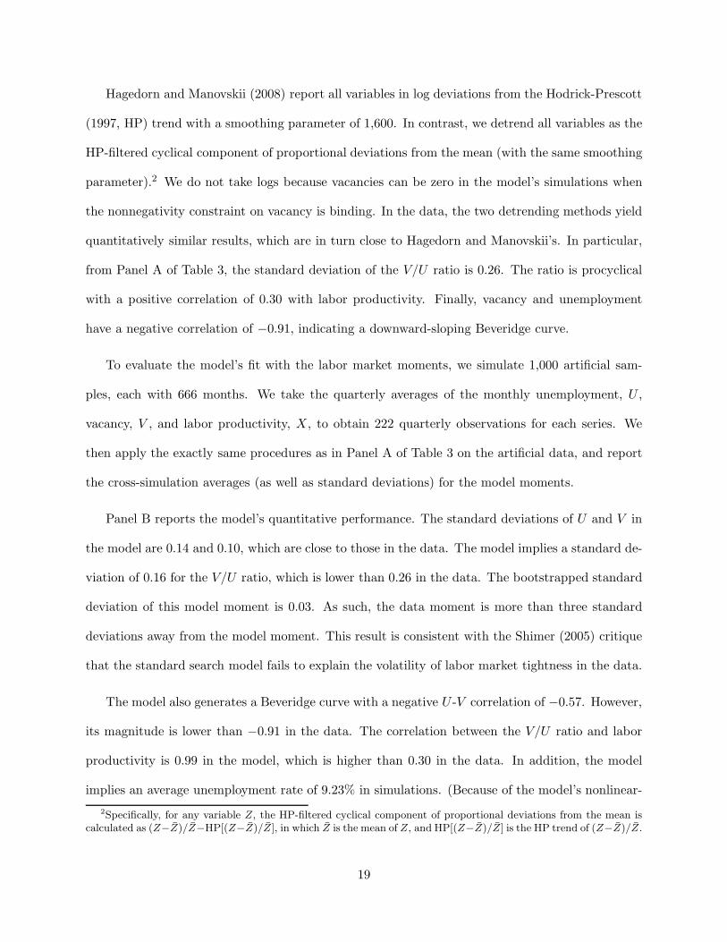
Hagedorn and Manovskii (2008) report all variables in log deviations from the Hodrick-Prescott

(1997, HP) trend with a smoothing parameter of 1,600. In contrast, we detrend all variables as the

HP-filtered cyclical component of proportional deviations from the mean (with the same smoothing

parameter).2 We do not take logs because vacancies can be zero in the model’s simulations when

the nonnegativity constraint on vacancy is binding. In the data, the two detrending methods yield

quantitatively similar results, which are in turn close to Hagedorn and Manovskii’s. In particular,

from Panel A of Table 3, the standard deviation of the V/U ratio is 0.26. The ratio is procyclical

with a positive correlation of 0.30 with labor productivity. Finally, vacancy and unemployment

have a negative correlation of −0.91, indicating a downward-sloping Beveridge curve.

To evaluate the model’s fit with the labor market moments, we simulate 1,000 artificial sam-

ples, each with 666 months. We take the quarterly averages of the monthly unemployment, U ,

vacancy, V , and labor productivity, X, to obtain 222 quarterly observations for each series. We

then apply the exactly same procedures as in Panel A of Table 3 on the artificial data, and report

the cross-simulation averages (as well as standard deviations) for the model moments.

Panel B reports the model’s quantitative performance. The standard deviations of U and V in

the model are 0.14 and 0.10, which are close to those in the data. The model implies a standard de-

viation of 0.16 for the V/U ratio, which is lower than 0.26 in the data. The bootstrapped standard

deviation of this model moment is 0.03. As such, the data moment is more than three standard

deviations away from the model moment. This result is consistent with the Shimer (2005) critique

that the standard search model fails to explain the volatility of labor market tightness in the data.

The model also generates a Beveridge curve with a negative U -V correlation of −0.57. However,

its magnitude is lower than −0.91 in the data. The correlation between the V/U ratio and labor

productivity is 0.99 in the model, which is higher than 0.30 in the data. In addition, the model

implies an average unemployment rate of 9.23% in simulations. (Because of the model’s nonlinear-

2Specifically, for any variable Z, the HP-filtered cyclical component of proportional deviations from the mean iscalculated as (Z−Z)/Z−HP[(Z−Z)/Z], in which Z is the mean of Z, and HP[(Z−Z)/Z] is the HP trend of (Z−Z)/Z.

19

Table 3 : Labor Market Moments

In Panel A, seasonally adjusted monthly unemployment (U , thousands of persons 16 years of ageand older) is from the Bureau of Labor Statistics. The seasonally adjusted help wanted advertisingindex, V , is from the Conference Board. The series are monthly from January 1951 to June 2006(666 months). Both U and V are converted to 222 quarterly averages of monthly series. Theaverage labor productivity, X, is seasonally adjusted real average output per person in the nonfarmbusiness sector from the Bureau of Labor Statistics. All variables are in HP-filtered proportionaldeviations from the mean with a smoothing parameter of 1,600. In Panel B, we simulate 1,000artificial samples, each of which has 666 monthly observations. We take the quarterly averagesof monthly U, V , and X to convert to 222 quarterly observations. We implement the exactlysame empirical procedures as in Panel A on these quarterly series, and report the cross-simulationaverages and standard deviations (in parentheses) for all the model moments.

U V V/U X

Panel A: Data

Standard deviation 0.119 0.134 0.255 0.012Quarterly autocorrelation 0.902 0.922 0.889 0.761

Correlation matrix −0.913 −0.801 −0.224 U0.865 0.388 V

0.299 V/U

Panel B: Model

Standard deviation 0.140 0.098 0.155 0.016(0.069) (0.019) (0.030) (0.002)

Quarterly autocorrelation 0.849 0.647 0.791 0.773(0.051) (0.061) (0.038) (0.040)

Correlation matrix −0.571 −0.696 −0.662 U(0.109) (0.131) (0.141)

0.920 0.948 V(0.049) (0.025)

0.994 V/U(0.015)

ity, the long-run average unemployment rate in simulations is somewhat lower than the calibration

target of 10%, which holds only roughly based on deterministic steady state relations.)

4.3 The Linkage between the Labor Market and the Financial Market

A large literature in financial economics shows that the equity risk premium is time-varying (and

countercyclical) in the data (e.g., Lettau and Ludvigson (2001)). In the labor market, as vacancy is

procyclical and unemployment is countercyclical, the V/U ratio is strongly procyclical (e.g., Shimer

(2005)). As such, the V/U ratio should forecast stock market excess returns with a negative slope

at business cycle frequencies. Panel A of Table 4 documents such predictability in the data.

20

Table 4 : Long-Horizon Regressions of Market Excess Returns on Labor Market Tightness

Panel A reports long-horizon regressions of log excess returns on the value-weighted market indexfrom CRSP,

∑Hh=1Rt+3+h −Rft+3+h, in which H is the forecast horizon in months. The regressors

are two-month lagged values of the V/U ratio. We report the ordinary least squares estimate of theslopes (Slope), the Newey-West corrected t-statistics (tNW ), and the adjusted R2s in percent. Theseasonally adjusted monthly unemployment (U , thousands of persons 16 years of age and older)is from the Bureau of Labor Statistics, and the seasonally adjusted help wanted advertising index(V ) is from the Conference Board. The sample is from January 1951 to June 2006 (666 monthlyobservations). We multiply the V/U series by 50 so that its average is close to that in the model. InPanel B, we simulate 1,000 artificial samples, each of which has 666 monthly observations. On eachartificial sample, we implement the exactly same empirical procedures as in Panel A, and reportthe cross-simulation averages and standard deviations (in parentheses) for all the model moments.

Forecast horizon (H) in months

1 3 6 12 24 36

Panel A: Data

Slope −1.425 −4.203 −7.298 −10.312 −9.015 −10.156tNW −2.575 −2.552 −2.264 −1.704 −0.970 −0.861Adjusted R2 0.950 2.598 3.782 3.672 1.533 1.405

Panel B: Model

Slope −0.807 −2.378 −4.610 −8.657 −15.378 −20.707(0.428) (1.244) (2.379) (4.416) (7.573) (9.799)

tNW −2.228 −2.341 −2.475 −2.776 −3.504 −4.138(0.800) (0.852) (0.925) (1.111) (1.508) (1.846)

Adjusted R2 0.692 2.035 3.915 7.323 13.000 17.568(0.463) (1.321) (2.489) (4.596) (7.890) (10.331)

Specifically, we perform monthly long-horizon regressions of log excess returns on the CRSP

value-weighted market returns,∑H

h=1Rt+3+h − Rft+3+h, in which H = 1, 3, 6, 12, 24, and 36 is the

forecast horizon in months. When H > 1, we use overlapping monthly observations of H-period

holding returns. The regressors are two-month lagged values of the V/U ratio. The BLS takes less

than one week to release monthly employment and unemployment data, and the Conference Board

takes about one month to release monthly help wanted advertising index data.3 We impose the

two-month lag between the V/U ratio and market excess returns to guard against look-ahead bias in

predictive regressions. To make the regression slopes comparable to those in the model, we also scale

up the V/U series in the data by a factor of 50 to make its average close to that in the model. This

scaling is necessary because the vacancy and unemployment series in the data have different units.

3We verify this practice through a private correspondence with the Conference Board staff.

21

Figure 2 : The Equity Risk Premium in Annual Percent, Et[Rt+1 −Rft+1]

−0.2

0

0.2

0

0.5

10

10

20

30

ProductivityEmployment

Panel A of Table 4 shows that the V/U ratio is a reliable forecaster of market excess returns. At

the one-month horizon, the slope is −1.43, which is more than 2.5 standard errors from zero. (The

standard errors are adjusted for heteroscedasticity and autocorrelations of 12 lags per Newey and

West (1987)). The adjusted R2 is close to 1%. The slopes are significant at the three-month and

six-month horizons but insignificant afterward. The adjusted R2s peak at 3.78% at the six-month

horizon, and decline to 3.67% at the one-year horizon and further to 1.41% at the three-year horizon.

To see how the model can explain this predictability, we plot in Figure 2 the equity risk premium

in annual percent on the state space of employment and productivity. We observe that the risk

premium is strongly countercyclical: it is low in good times when both employment and productiv-

ity are high, but high in bad times when both employment and productivity are low. As shown in

Panel A of Figure 1, the labor market tightness, Vt/Ut, is strongly procyclical: it is low in bad times

(the high-unemployment-low-productivity states), but high in good times (the low-unemployment-

high-productivity states). The joint cyclical properties of the equity premium and the V/U ratio

imply that V/U should forecast market excess returns with a negative slope in the model.

Panel B of Table 4 reports the model’s quantitative fit for the predictive regressions. Consistent

with the data, the model predicts that the V/U ratio forecasts market excess returns with a negative

22

slope. In particular, at the one-month horizon, the predictive slope is −0.81 with a t-statistic of

−2.23. At the six-month horizon, the slope is −4.61 with a t-statistic of −2.38. However, the model

implies stronger predictive power for the V/U ratio than that in the data. Both the t-statistic of

the slope and the adjusted R2 increase monotonically with the forecast horizon. In contrast, both

statistics peak at the six-month horizon but decline afterward in the data.

Panel A of Figure 3 plots the cross-correlations and their two standard-error bounds between the

V/U ratio, Vt/Ut, and future market excess returns, Rt+H−Rft+H , forH = 1, 2, . . . , 36 months in the

data. No overlapping observations are used. The panel shows that the correlations are significantly

negative for forecast horizons up to six months, consistent with the predictive regressions in

Table 4. Panel B reports the cross-correlations and their two cross-simulation standard-deviation

bounds from the model’s bootstrapped distribution. Consistent with the data, the model

predicts significantly negative cross-correlations between Vt/Ut and future market excess returns

for short horizons. However, although the cross-correlations are insignificant at long horizons, the

correlations decay more slowly than those in the data, consistent with Panel B of Table 4.

4.4 Endogenous Rare Disasters

The search economy gives rise endogenously to rare disaster risks a la Rietz (1988) and Barro

(2006). We simulate 1,006,000 monthly periods from the model, discard the first 6,000 periods,

and treat the remaining one million months as the model’s stationary distribution. Figure 4 reports

the empirical cumulative distribution functions for unemployment, output, consumption, and div-

idend. From Panel A, unemployment is positively skewed with a long right tail. As the population

moments, the mean unemployment rate is 9.23%, the median is 8.05%, and the skewness is 7.46.

The 2.5 percentile of unemployment is close to the median, 6.34%, whereas the 97.5 percentile is

far away, 19.97%. As a mirror image, the employment rate is negatively skewed with a long left

tail. As a result, output, consumption, and dividend all show infrequent but deep disasters (Panels

B–D). With small probabilities, the economy falls off the cliff in simulations.

23

Figure 3 : Cross-Correlations between the V/U Ratio and Future Market Excess Returns

We report the cross-correlations (in red) between labor market tightness, Vt/Ut, and future market

excess returns, Rt+H−Rft+H , in which H = 1, 2, . . . , 36 is the forecast horizon in months, as well astheir two standard-error bounds (in blue broken lines). In Panel A, Vt is the seasonally adjusted helpwanted advertising index from the Conference Board, and Ut is the seasonally adjusted monthlyunemployment (thousands of persons 16 years of age and older) from the BLS. The sample isfrom January 1951 to June 2006. The market excess returns are the CRSP value-weighted marketreturns in excess of one-month Treasury bill rates. In Panel B, we simulate 1,000 artificial samples,each with 666 monthly observations. On each artificial sample, we calculate the cross-correlationsbetween Vt/Ut and Rt+H −Rft+H , and plot the cross-simulation averaged correlations (in red) andtheir two cross-simulation standard-deviation bounds (in blue broken lines).

Panel A: Data Panel B: Model

0 10 20 30 40−0.2

−0.1

0

0.1

0.2

Forecast horizon0 10 20 30 40

−0.2

−0.1

0

0.1

0.2

Forecast horizon

The disasters in macroeconomic quantities reflect in asset prices as rare upward spikes in the eq-

uity risk premium, Et[Rt+1 −Rft+1]. From Figure 5, its stationary distribution is positively skewed

with a long right tail. The mean risk premium is 5.02% per annum, and its 2.5 and 97.5 percentiles

are 1.63% and 8.93%, respectively. However, with small probabilities, the risk premium can reach

very high levels: the maximum equity premium is close to 23% in simulations.

Do macroeconomic disasters arising endogenously from the model resemble those in the data?

Barro and Ursua (2008) apply a peak-to-trough method on samples from 1870 to 2006 to identify

economic crises, defined as cumulative fractional declines in per capita consumption or GDP of at

least 10%. Suppose there are two states, normalcy and disaster. The disaster probability measures

the likelihood with which the economy shifts from normalcy to disaster in a given year. The number

24

Figure 4 : Empirical Stationary Distribution of the Model: Unemployment, Output,Consumption, and Dividend

Panel A: Unemployment Panel B: Output

0 0.2 0.4 0.6 0.8 10

0.2

0.4

0.6

0.8

1

Unemployment

Pro

babi

lity

0 0.5 1 1.50

0.2

0.4

0.6

0.8

1

Output

Pro

babi

lity

Panel C: Consumption Panel D: Dividend

0 0.2 0.4 0.6 0.8 10

0.2

0.4

0.6

0.8

1

Consumption

Pro

babi

lity

−0.08 −0.06 −0.04 −0.02 0 0.02 0.040

0.2

0.4

0.6

0.8

1

Dividend

Pro

babi

lity

of disaster years is defined as the number of years in the interval between peak and trough for each

disaster event. The number of normalcy years is the total number of years in the sample minus

the number of disaster years. The disaster probability is the ratio of the number of disasters over

the number of normalcy years. Barro and Ursua estimate the disaster probability to be 3.63%, the

average size 22%, and the average duration 3.6 years for consumption disasters. For GDP disasters,

the disaster probability is 3.69%, the average size 21%, and the average duration 3.5 years.

To quantify the magnitude of the disasters in the model, we first simulate the economy for 6,000

monthly periods to reach the stationary distribution. We then repeatedly simulate 1,000 artificial

25

Figure 5 : Empirical Stationary Distribution of the Model: The Equity Risk Premium

0 5 10 15 20 250

0.2

0.4

0.6

0.8

1

The equity risk premium

Pro

babi

lity

samples, each with 1,644 months (137 years). The sample size matches the average sample size in

Barro and Ursua (2008). On each artificial sample, we time-aggregate the monthly observations of

consumption and output into annual observations. We apply Barro and Ursua’s measurement on

each artificial sample, and report the cross-simulation averages and the 5 and 95 percentiles for the

disaster probability, size, and duration for both consumption and GDP (output) disasters.

Table 5 reports the detailed results. From Panel A (consumption disasters), the disaster prob-

ability and the average disaster size in the model are close to those in the data, but the average

duration is somewhat higher in the model. The disaster probability is 3.22%, which is close to

3.63% in the data. The average size of the disasters in the model is 19.7%, which is close to 22% in

the data. The average duration is 4.81 years, which is longer than 3.6 years in the data. However,

the cross-simulation standard deviation of the average duration is 1.21, meaning that the data

duration is about one standard deviation from the model’s estimate.

From Panel B of Table 5, the average size of GDP disasters in the model, 18.84%, is close to

that in the data, 21%. However, the disaster probability of 4.94% is higher than 3.69% in the data.

The cross-simulation standard deviation of the GDP disaster probability is 2.01%, meaning that

the probability in the data is within one standard deviation from the model’s estimate. In addition,

the average duration of the GDP disasters in the model is 4.47 years, which is longer than 3.5 years

26

Table 5 : Moments of Macroeconomic Disasters

The data moments are from Barro and Ursua (2008). The model moments are from 1,000simulations, each with 1,644 monthly observations. We time-aggregate these monthly observationsof consumption and output into 137 annual observations. On each artificial sample, we apply Barroand Ursua’s peak-to-trough method to identify economic crises, defined as cumulative fractionaldeclines in per capita consumption or GDP of at least 10%. We report the mean and the 5 and95 percentiles across the 1,000 simulations. The p-values are the percentages with which a givenmodel moment is higher than its data moment. The disaster probabilities and average size are allin percent, and the average duration is in terms of years.

Data Model

Mean 5% 95% p-value

Panel A: Consumption disasters

Probability 3.63 3.22 0.76 6.42 0.33Average size 22 19.70 11.44 37.45 0.23Average duration 3.6 4.81 3.00 7.00 0.84

Panel B: GDP disasters

Probability 3.69 4.94 1.61 8.59 0.32Average size 21 18.84 12.42 32.63 0.27Average duration 3.5 4.47 3.25 6.00 0.86

in the data. The cross-simulation standard deviation of the duration is 0.84 years, meaning that

the duration in the data is slightly more than one standard deviation from the model’s estimate.

Figure 6 reports the frequency distributions of consumption and GDP disasters by size and

duration based on 1,000 simulations of the model. This figure is the model’s counterpart to Fig-

ures 1 and 2 in Barro and Ursua (2008). We see that the size and duration distributions for both

consumption and GDP disasters display largely similar patterns as those in the data. In particular,

the size distributions seem to follow a power-law density as emphasized by Barro and Jin (2011).

4.5 Endogenous Long Run Risks and Endogenous Uncertainty Risks

In this subsection, we explore the model’s implications for long run risks and uncertainty shocks.

Bansal and Yaron (2004) propose long-run consumption risks as a mechanism for explaining aggre-

27

Figure 6 : Distributions of Consumption and GDP Disasters by Size and Duration

Panel A: Consumption disasters by size Panel B: Consumption disasters by duration

0 0.2 0.4 0.6 0.8 10

1

2

3

4

Num

ber

of d

isas

ters

Cumulative fractional decline in consumption1 2 3 4 5 6 7 8 9 10

0

0.5

1

1.5

Num

ber

of c

onsu

mpt

ion

disa

ster

s

Duration (years from peak to trough)

Panel C: GDP disasters by size Panel D: GDP disasters by duration

0 0.2 0.4 0.6 0.8 10

1

2

3

4

Num

ber

of d

isas

ters

Cumulative fractional decline in output1 2 3 4 5 6 7 8 9 10

0

0.5

1

1.5

Num

ber

of o

utpu

t dis

aste

rs

Duration (years from peak to trough)

gate asset prices. Bansal and Yaron specify the following exogenous consumption growth process:

zt+1 = .979zt + .044σtet+1, (26)

gt+1 = .0015 + zt + σtηt+1, (27)

σ2t+1 = .00782 + .987(σ2t − σ2) + .23 × 10−5wt+1, (28)

in which gt+1 is the consumption growth, zt is the expected consumption growth, σt is the con-

ditional volatility of gt+1, and et+1, ut+1, ηt+1, and wt+1, are i.i.d. standard normal shocks, which

are mutually uncorrelated. Bansal and Yaron argue that the stochastic slow-moving component,

28

zt, of the consumption growth is crucial for explaining the level of the equity premium, and that

the mean-reverting stochastic volatility helps explain the time-variation in the risk premium.

Kaltenbrunner and Lochstoer (2010) lend support to Bansal and Yaron’s (2004) long-run risks

argument by showing that these risks can arise endogenously via consumption smoothing. Within

a production economy with capital as the only productive input, Kaltenbrunner and Lochstoer

(Table 6) show that the (monthly) consumption growth follows:

zt+1 = .986zt + .093σet+1, (29)

gt+1 = .0013 + zt + σηt+1, (30)

with transitory productivity shocks. With permanent productivity shocks, the zt process follows:

zt+1 = .990zt + .247σet+1. (31)

However, their economies fail to generate heteroscedasticity in shocks to expected and realized

consumption growth (see their footnote 15). Also, the permanent shocks model produces an equity

premium very close to zero. Although the transitory shocks model offers a high equity premium,

its calibration includes a time discount factor that is larger than unity.

We ask how consumption dynamics in the search economy compare with those in the

Kaltenbrunner and Lochstoer (2010) economy and with those calibrated in Bansal and Yaron

(2004). This question is interesting because different parameterizations of the consumption process

specified in equations (26)–(28) can be consistent with simple moments of consumption growth

such as volatility and autocorrelations (see Table 2). Yet, different parameterizations can imply

very different economic mechanisms for the equity risk premium and its time-variation.

We simulate the search economy for 6,000 monthly periods to reach the stationary distribution,

and then simulate one million monthly periods. We calculate the expected consumption growth

and the conditional volatility of the realized consumption growth on the employment-productivity

29

grid, and use the solutions to simulate these moments. Fitting the consumption growth process

specified by Bansal and Yaron (2004) on the simulated data, we obtain:

zt+1 = .700zt + .570σtet+1, (32)

gt+1 = zt + σtηt+1, (33)

σ2t+1 = .00632 + .908(σ2t − σ2) + 1.93× 10−5wt+1. (34)

In addition, the unconditional correlation between et+1 and ηt+1 is 0.26, and the correlations be-

tween et+1 and wt+1 and between ηt+1 and wt+1 are close to zero.

Although the consumption growth is not i.i.d. in our economy, the persistence in the expected

consumption growth is only 0.70, which is lower than that in Kaltenbrunner and Lochstoer (2010)

and that calibrated in Bansal and Yaron (2004). However, the expected consumption growth is more

volatile in our economy. The conditional volatility of the expected consumption growth is 57% of the

conditional volatility of the realized consumption growth. This percentage is substantially higher

than 9.3% and 24.7% in Kaltenbrunner and Lochstoer as well as 4.4% in Bansal and Yaron. For

the stochastic variance, its persistence is 0.908 in our economy, which is lower than 0.987 in Bansal

and Yaron. However, the volatility of our stochastic variance is more than eight times of theirs.

We interpret these results as saying that disasters risks play a more important role than long-

run risks (in the sense of extreme persistence of expected consumption growth) in our economy.

Because the economy occasionally falls into disasters, shocks to both expected consumption growth

and the conditional variance of consumption growth are magnified. Disasters also give rise to lower

persistence for the expected consumption growth and the conditional variance.

To further characterize the endogenous uncertainty risks in our economy, we plot the conditional

market volatility, σRt , on the employment-productivity grid. From Panel A of Figure 7, the market

volatility is strongly countercyclical: it is low in good times and high in bad times. Panel B reports

the empirical cumulative distribution of the market volatility in simulations. We simulate 1,006,000

30

Figure 7 : The Conditional Market Volatility in Annual Percent, σRt , on the Grid and

Empirical Stationary Distribution in Simulations

Panel A: On the grid Panel B: Stationary distribution

−0.2

0

0.2

0

0.5

10

20

40

60

80

ProductivityEmployment0 10 20 30 40

0

0.2

0.4

0.6

0.8

1

The conditional market volatility

Pro

babi

lity

monthly periods, discard the first 6,000 periods, and treat the remaining one million periods as

from the stationary distribution. The conditional volatility hovers around its median about 10%

per annum. However, with small probabilities, the market volatility can jump to more than 30%.

4.6 Procyclical Dividend Dynamics

Kaltenbrunner and Lochstoer (2010) show that dividend is countercyclical in the standard pro-

duction economy with capital as the only productive input (see also Jermann (1998)). Intuitively,

dividend roughly equals profits minus investment, and profits in turn roughly equal output minus

wages. Without labor market frictions, the wage rate equals the marginal product of labor, meaning

that profits are proportional to (and as procyclical as) output. Because investment is more pro-

cylical than output (and profits), dividend, as profits minus investment, has to be countercyclical.

The dividend countercyclicality in the baseline production economy is counterfactual. Dividend

in the model corresponds with net payout (dividend plus stock repurchases minus new equity issues)

in the data. Following Jermann and Quadrini (2010), we measure net payout using aggregate data

from the Flow of Funds Accounts of the Federal Reserve Board.4 The sample is quarterly from the

4Specifically, we calculate net payout as net dividends of nonfarm, nonfinancial business (Table F.102, line 3) plusnet dividends of farm business (Table F.7, line 24) minus net increase in corporate equities of nonfinancial business(Table F.101, line 35) minus proprietors’ net investment of nonfinancial business (Table F.101, line 39).

31

fourth quarter of 1951 to the fourth quarter of 2010. We obtain quarterly real GDP (NIPA Table

1.1.6) and quarterly implicit price deflator for GDP (NIPA Table 1.1.9) used to deflate net payout.

We detrend real net payout and real GDP as HP-filtered proportional deviations from the mean

with a smoothing parameter of 1,600. We do not take logs because net payout can be negative in

the data. Consistent with Jermann and Quadrini, we find that the cyclical components of real net

payout and real GDP have a positive correlation of 0.55.

The search economy avoids the pitfall of counterfactual dividend dynamics. Intuitively, the

wage rate from the generalized Nash bargaining process is no longer equal to the marginal product

of labor. Because the value of unemployment activities, b, is positive, wages are less procyclical than

productivity. As such, profits are more procyclical than output. In effect, the relatively inelastic

wage rate works as operating leverage to magnify the procyclicality (and volatility) of profits. This

turbocharged procyclicality of profits is sufficient to overcome the procyclicality of total vacancy

costs, κVt, so as to produce procyclical dividend dynamics.

Quantitatively, the model also succeeds in replicating the procyclicality of dividend. We first

simulate the economy for 6,000 monthly periods to reach the stationary distribution, and then

repeatedly simulate 1,000 artificial samples, each with 711 months (237 quarters). The sample size

matches the quarterly series from the fourth quarter of 1951 to the fourth quarter of 2010. On each

artificial sample, we time-aggregate monthly observations of dividend and output into quarterly

observations. After detrending the quarterly series as HP-filtered propertional deviations from the

mean, we calculate the correlation between the cyclical components of dividend and output. We

find that this correlation to be 0.53 in the model, with a cross-simulation standard deviation of

0.14, thereby replicating the correlation of 0.55 in the data.

We also compare the wage dynamics in the model to those in the data. Following Hagedorn

and Manovskii (2008), we measure wages as labor share times labor productivity from BLS. The

sample is quarterly from the first quarter of 1947 to the four quarter of 2010 (256 quarters). We

32

take logs and HP-detrend the series with a smoothing parameter of 1,600. We find that the wage

elasticity to labor productivity is 0.46, close to Hagedorn and Manovskii’s estimate, meaning that

a one percentage point increase in labor productivity delivers a 0.46 percentage increase in real

wages. In addition, we measure (quarterly) output as real GDP (NIPA Table 1.1.6). We find that

the correlation between the log wage growth and the log output growth is 0.48, and that the ratio

of the wage growth volatility over the output growth volatility is 0.70.

To see the model’s performance, we first simulate the economy for 6,000 monthly periods to

reach the stationary distribution, and then repeatedly simulate 1,000 artificial samples, each with

768 months (256 quarters). On each artificial sample, we take quarterly averages of monthly wages

and labor productivity to obtain quarterly series. Implementing the same empirical procedure used

on the real data, we find that the wage elasticity to productivity is 0.56 in the model, which is not

far from 0.46 in the data. However, the correlation between the log wage growth and the log output

growth in the model is 0.90, which is too high relative to 0.48 in the data. At the same time, the

relative volatility of the wage growth is 0.36, which is too low relative to 0.70 in the data.

4.7 Comparative Statics

To shed further light on the economic mechanisms underlying the risk premium in the model, we

conduct several comparative statics by varying the model’s key parameters. Table 6 reports four

experiments: (i) the value of unemployment activities, b, changed from 0.85 in the benchmark cali-

bration to 0.4; (ii) the job separation rate, s, from 0.05 to 0.035; (iii) the vacancy cost, κ, from 0.975

to 0.2; and (iv) the workers’ bargaining power, η, from 0.052 to 0.10. In each experiment, except for

the parameter in question, all the other parameters are the same as in the benchmark calibration.

The Value of Unemployment Activities

In the first experiment, the value of unemployment activities, b = 0.4, is set to be the parameter

value in Shimer (2005). Because unemployment is less valuable to workers, the unemployment rate

drops to 5.17%. A lower b also means that the wage rate is more sensitive to shocks. As such,

33

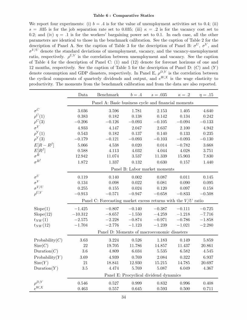
Table 6 : Comparative Statics

We report four experiments: (i) b = .4 is for the value of unemployment activities set to 0.4; (ii)s = .035 is for the job separation rate set to 0.035; (iii) κ = .2 is for the vacancy cost set to0.2; and (iv) η = .1 is for the workers’ bargaining power set to 0.1. In each case, all the otherparameters are identical to those in the benchmark calibration. See the caption of Table 2 for thedescription of Panel A. See the caption of Table 3 for the description of Panel B: σU , σV , andσV/U denote the standard deviations of unemployment, vacancy, and the vacancy-unemploymentratio, respectively. ρU,V is the correlation between unemployment and vacancy. See the captionof Table 4 for the description of Panel C: (1) and (12) denote for forecast horizons of one and12 months, respectively. See the caption of Table 5 for the description of Panel D: (C) and (Y )denote consumption and GDP disasters, respectively. In Panel E, ρD,Y is the correlation betweenthe cyclical components of quarterly dividends and output, and eW,X is the wage elasticity toproductivity. The moments from the benchmark calibration and from the data are also reported.

Data Benchmark b = .4 s = .035 κ = .2 η = .15

Panel A: Basic business cycle and financial moments

σC 3.036 3.596 1.781 2.153 1.405 4.640ρC(1) 0.383 0.182 0.138 0.142 0.134 0.242ρC(3) −0.206 −0.126 −0.093 −0.105 −0.094 −0.133

σY 4.933 4.147 2.047 2.637 2.100 4.942ρY (1) 0.543 0.182 0.137 0.140 0.133 0.235ρY (3) −0.179 −0.121 −0.093 −0.103 −0.093 −0.130

E[R−Rf ] 5.066 4.538 0.020 0.014 −0.782 3.668E[Rf ] 0.588 4.113 4.032 4.044 4.028 3.751σR 12.942 11.074 3.537 11.339 15.903 7.830

σRf

1.872 1.337 0.132 0.630 0.157 1.440

Panel B: Labor market moments

σU 0.119 0.140 0.002 0.087 0.011 0.145σV 0.134 0.098 0.022 0.081 0.090 0.095

σV/U 0.255 0.155 0.024 0.120 0.097 0.158ρU,V −0.913 −0.571 −0.947 −0.658 −0.833 −0.508

Panel C: Forecasting market excess returns with the V/U ratio

Slope(1) −1.425 −0.807 −0.140 −0.387 −0.111 −0.725Slope(12) −10.312 −8.657 −1.550 −4.259 −1.218 −7.716tNW (1) −2.575 −2.228 −0.874 −0.971 −0.786 −1.858tNW (12) −1.704 −2.776 −1.123 −1.239 −1.021 −2.280

Panel D: Moments of macroeconomic disasters

Probability(C) 3.63 3.224 0.526 1.183 0.149 5.859Size(C) 22 19.705 11.786 14.857 11.437 20.861Duration(C) 3.6 4.809 6.034 5.535 6.582 4.545

Probability(Y ) 3.69 4.939 0.769 2.084 0.322 6.937Size(Y ) 21 18.841 12.930 15.215 14.785 20.697Duration(Y ) 3.5 4.474 5.769 5.087 6.049 4.367

Panel E: Procyclical dividend dynamics

ρD,Y 0.546 0.527 0.999 0.832 0.996 0.408eW,X 0.463 0.557 0.645 0.593 0.500 0.711

34

the wage elasticity to productivity increases to 0.65 from 0.56 in the benchmark economy. As a

result of the higher wage elasticity to productivity, profits and vacancies are less sensitive to shocks.

Employment and output are also less sensitive, giving rise to a low consumption growth volatility

of 1.78% per annum and a low output growth volatility of 2.05% (Panel A of Table 6).

The low-b economy shows essentially no disaster risks. From the stationary distributions re-

ported in Figure 8, the unemployment rate varies within a narrow range close to 5%. Neither

output nor consumption has a long left tail in its empirical cumulative distribution. Using Barro

and Ursua’s (2008) peak-to-trough measurement, Panel D of Table 6 shows that the disaster proba-

bilities are less than 0.8%, and the average size of the disasters are less than 13%. Because of the lack

of disaster risks, the equity premium drops to slightly above zero, and is largely time-invariant: the

V/U ratio shows no predictive power for market excess returns. The market volatility also drops.

Consistent with Shimer (2005), the standard deviation of the V/U ratio in the low-b model is

only 0.02, which is an order of magnitude smaller than 0.26 in the data. As such, a high value of

unemployment activities helps alleviate simultaneously the Shimer puzzle and the equity premium

puzzle. Intuitively, by dampening the procyclical covariation of wages with productivity, a high

value of b magnifies the procyclical variation of profits and vacancies, so as to increase the volatility

of the V/U ratio. At the same time, the high value of b also turbocharges the procyclical variation

of dividend, so as to raise the equity risk premium and the stock return volatility.

The Job Separation Rate

In the second experiment, we reduce the job separation rate, s, from 0.05 to 0.035. Because the

productive input in the economy is destructed at a lower rate, the disasters in the low-s economy

are less extreme and less frequent than those in the benchmark economy. The consumption and

GDP disaster probabilities are 1.18% and 2.08%, respectively, which are more than halved relative

to those in the benchmark economy. The average magnitudes of consumption and GDP disasters

are also lower: 14.86% and 15.22% versus 19.71% and 18.84%, respectively. The low-s economy

35

Figure 8 : Empirical Cumulative Distribution Functions, the Model with a Low Value ofUnemployment Activities, b = 0.40

Panel A: Unemployment Panel B: Output

0.05 0.051 0.052 0.053 0.054 0.0550

0.2

0.4

0.6

0.8

1

Unemployment

Pro

babi

lity

0.8 0.9 1 1.1 1.2 1.30

0.2

0.4

0.6

0.8

1

Output

Pro

babi

lity

Panel C: Consumption Panel D: The equity premium

0.55 0.6 0.65 0.7 0.75 0.80

0.2

0.4

0.6

0.8

1

Consumption

Pro

babi

lity

0.08 0.081 0.082 0.083 0.0840

0.2

0.4

0.6

0.8

1

The equity risk premium

Pro

babi

lity

also has a lower consumption growth volatility than the benchmark economy: 2.15 versus 3.60% per

annum. Because of the lower consumption volatility and the dampened disaster risks, the equity

risk premium is close to zero and largely time-invariant in the low-s economy.

The Vacancy Cost

In the third experiment, we reduce the vacancy cost parameter, κ, from 0.975 in the benchmark

economy to 0.2, which is close to the value in Shimer (2005). Lower vacancy costs mean that

the firm is more capable of smoothing the impact of exogenous productivity shocks by varying

vacancies. As such, the output growth volatility falls to 2.1% per annum, and the consumption

36

growth volatility to 1.41%. Both consumption and GDP disaster probabilities are close to zero.

As a result, the equity premium is close to zero, even slightly negative. However, lower vacancy

costs imply that both vacancies and the marginal value of posting vacancies are more sensitive to

shocks. From the definition of the stock return in equation (15), the heightened sensitivity of the

marginal value translates to a higher market volatility.

The Workers’ Bargaining Weight

In the final experiment, we increase the workers’ bargaining weight, η, from 0.052 to 0.10. A higher

η makes wages more procyclical and profits less procyclical. Dividend is also less procyclical. This

effect weakens operating leverage, and lowers the equity risk premium. However, the high-η econ-

omy shows more volatile consumption growth and output growth than the benchmark economy.

Because wages are more procyclical and profits are less procyclical, vacancies are less responsive to

shocks. As such, unemployment (and thus employment) are more responsive to shocks, making out-

put more responsive to shocks as well. From the resource constraint in equation (21), consumption

must then absorb more shocks to become more volatile.

5 Conclusion

We study aggregate asset pricing by embedding the standard Diamond-Mortensen-Pissarides search

model of the labor market into a dynamic stochastic general equilibrium economy. We find that

search frictions in the labor market help explain the equity premium in the financial market. With

reasonable parameter values, the model reproduces a sizeable equity risk premium with a low inter-

est rate volatility. The equity premium is also strongly countercyclical, and is forecastable by labor

market tightness, a prediction that we confirm in the data. Intriguingly, search frictions create

endogenously rare disaster risks as emphasized by Rietz (1988) and Barro (2006).

37

References

Andolfatto, David, 1996, Business cycles and labor-market search, American Economic Review

86, 112–132.

Bansal, Ravi, and Amir Yaron, 2004, Risks for the long run: A potential resolution of asset pricingpuzzles, Journal of Finance 59, 1481–1509.

Barro, Robert J., 2006, Rare disasters and asset markets in the twentieth century, Quarterly

Journal of Economics 121, 823–866.

Barro, Robert J., 2009, Rare disasters, asset prices, and welfare costs, American Economic Review

99, 243–264.

Barro, Robert J., and Tao Jin, 2011, On the size distribution of macroeconomic disasters,Econometrica 79, 1567–1589.

Barro, Robert J., and Jose F. Ursua, 2008, Macroeconomic crises since 1870, Brookings Papers onEconomic Activity 1, 255–335.

Bazdresch, Santiago, Frederico Belo, and Xiaoji Lin, 2009, Labor hiring, investment, and stockreturn predictability in the cross section, working paper, University of Minnesota.

Boldrin, Michele, Lawrence J. Christiano, and Jonas D. M. Fisher, 2001, Habit persistence, assetreturns, and the business cycle, American Economic Review 91, 149–166.

Campanale, Claudio, Rui Castro, and Gian Luca Clementi, 2010, Asset pricing in a productioneconomy with Chew-Dekel preferences, Review of Economic Dynamics 13, 379–402.

Campbell, John Y., and John H. Cochrane, 1999, By force of habit: A consumption-basedexplanation of aggregate stock market behavior, Journal of Political Economy 107, 205–251.

Christiano, Lawrence J., and Jonas D. M. Fisher, 2000, Algorithms for solving dynamic modelswith occasionally binding constraints, Journal of Economic Dynamics and Control 24, 1179–1232.

Clark, Kim B., 1990, Unemployment insurance and labor market transitions, in Understanding

Unemployment, Lawrence Summers, ed. MIT Press, Cambridge Massachusetts.

Danthine, Jean-Pierre, and John B. Donaldson, 2002, Labour relations and asset returns, Reviewof Economic Studies 69, 41–64.

Davis, Steven J., R. Jason Faberman, John Haltiwanger, 2006, The flow approach to labor markets:New data sources and micro-macro links, Journal of Economic Perspectives 20, 3–26.

Den Haan, Wouter J., Garey Ramey, and Joel Watson, 2000, Job destruction and propagation ofshocks, American Economic Review 90, 482–498.

Diamond, Peter A., 1982, Wage determination and efficiency in search equilibrium, Review of

Economic Studies 49, 217–227.

Epstein, Larry G., and Stanley E. Zin, 1989, Substitution, risk aversion, and the temporal behaviorof consumption and asset returns: A theoretical framework, Econometrica 57, 937–969.

38

Favilukis, Jack, and Xiaoji Lin, 2011, Infrequent renegotiation of wages: A solution to severalasset pricing puzzles, working paper, The Ohio State University.

Frank, Murray Z., and Vidhan K. Goyal, 2008, Trade-off and pecking order theories of debt,in Handbook of Corporate Finance: Empirical Corporate Finance edited by Espen Eckbo,Volume 2, 135–202, Elsevier Science, North Holland.

Gabaix, Xavier, 2009, Fixing the asset pricing properties of RBC models with variable raredisasters, working paper, New York University.

Gertler, Mark, and Antonella Trigari, 2009, Unemployment fluctuations with staggered Nash wagebargaining, Journal of Political Economy 117, 38–86.

Gourio, Francois, 2010, Disaster risk and business cycles, forthcoming, American Economic

Review.

Guvenen, Fatih, 2009, A parsimonious macroeconomic model for asset pricing, Econometrica 77,1711–1750.

Hagedorn, Marcus, and Iourii Manovskii, 2008, The cyclical behavior of equilibrium unemploymentand vacancies revisited, American Economic Review 98, 1692–1706.

Hall, Robert E., 2005, Employment fluctuations with equilibrium wage stickiness, 2005, American

Economic Review 95, 50–65.

Hodrick, Robert J., and Edward C. Prescott, 1997, Postwar U.S. business cycles: An empiricalinvestigation, Journal of Money, Credit, and Banking 29, 1–16.

Jermann, Urban J., 1998, Asset pricing in production economies, Journal of Monetary Economics

41, 257–275.

Jermann, Urban J., and Vincenzo Quadrini, 2010, Macroeconomic effects of financial shocks,forthcoming, American Economic Review.

Kaltenbrunner, Georg, and Lars Lochstoer, 2010, Long-run risk through consumption smoothing,Review of Financial Studies 23, 3190–3224.

Kopecky, Karen A., and Richard M. H. Suen, 2010, Finite state Markov-chain approximations tohighly persistent processes, Review of Economic Dynamics 13, 701–714.

Krause, Michael U., and Thomas A. Lubik, 2007, The (ir)relevance of real wage rigidity in thenew Keynesian model with search frictions, Journal of Monetary Economics 54, 706–727.

Lettau, Martin, and Sydney Ludvigson, 2001, Consumption, aggregate wealth, and expected stockreturns, Journal of Finance 56, 815–849.

Liu, Laura Xiaolei, Toni M. Whited, and Lu Zhang, 2009, Investment-based expected stockreturns, Journal of Political Economy 117, 1105–1139.

Merz, Monika, 1995, Search in labor market and the real business cycle, Journal of Monetary

Economics 95, 269–300.

39

Merz, Monika, and Eran Yashiv, 2007, Labor and the market value of the firm, American Economic

Review 97, 1419–1431.

Miranda, Mario J., and Paul L. Fackler, 2002, Applied Computational Economics and Finance,The MIT Press, Cambridge, Massachusetts.

Mortensen, Dale T., 1982, The matching process as a noncooperative bargaining game, in J. J.McCall, ed., The Economics of Information and Uncertainty, Chicago: University of ChicagoPress, 233–254.

Newey, Whitney K., and Kenneth D. West, 1987, A simple, positive semi-definite,heteroskedasticity and autocorrelation consistent covariance matrix, Econometrica 55, 703–708.

Petrongolo, Barbara, and Christopher A. Pissarides, 2001, Looking into the black box: A surveyof the matching function, Journal of Economic Literature 39, 390–431.

Pissarides, Christopher A., 1985, Short-run dynamics of unemployment, vacancies, and real wages,American Economic Review 75, 676–690.

Pissarides, Christopher A., 2000, Equilibrium Unemployment Theory 2nd ed., Cambridge MA:MIT Press.

Reinhart, Carmen M., and Kenneth Rogoff, 2009, This Time is Different: Eight Centuries of

Financial Folly, Princeton: Princeton University Press.

Rietz, Thomas A., 1988, The equity risk premium: A solution, Journal of Monetary Economics

22, 117–131.

Rouwenhorst, K. Geert, 1995, Asset pricing implications of equilibrium business cycle models, inT. Cooley ed., Frontiers of Business Cycle Research, Princeton: Princeton University Press,294–330.

Shimer, Robert, 2005, The cyclical behavior of equilibrium unemployment and vacancies,American Economic Review 95, 25–49.

Tallarini, Thomas D., 2000, Risk-sensitive real business cycles, Journal of Monetary Economics

45, 507–532.

40

A The Stock Return Equation

We prove equation (15) following an analogous proof in Liu, Whited, and Zhang (2009) in the

context of the q-theory of investment. Rewrite the equity value maximization problem as:

St = max{Vt+τ ,Nt+τ+1}

Et

∞∑

τ=0

Mt+τ

Xt+τNt+τ −Wt+τNt+τ − κVt+τ

−µt+τ [Nt+τ+1 − (1− s)Nt+τ

−Vt+τq(θt+τ )] + λt+τq(θt+τ )Vt+τ

, (A.1)

in which µt is the Lagrange multiplier on the employment accumulation equation, and λt is the

Lagrange multiplier on the irreversibility constraint on job creation. The first order conditions are

equations (10) and (11), and the Kuhn-Tucker condition is equation (14).

Define dividends as Dt = XtNt−WtNt−κVt and the ex-dividend equity value as Pt = St−Dt.

Expanding St yields:

Pt +XtNt −WtNt − κVt = St = XtNt −WtNt − κVt − µt [Nt+1 − (1− s)Nt − Vtq(θt)] + λtq(θt)Vt

+EtMt+1

[

Xt+1Nt+1 −Wt+1Nt+1 − κVt+1 − µt+1 [Nt+2 − (1− s)Nt+1 − Vt+1q(θt+1)]

+λt+1q(θt+1)Vt+1] + . . . (A.2)

Recursively substituting equations (10) and (11) yields: Pt+XtNt−WtNt−κVt = XtNt−WtNt+

µt(1−s)Nt. Using equation (10) to simplify further: Pt = κVt+µt(1−s)Nt = µt[(1−s)Nt+q(θt)Vt]+

λtq(θt)Vt = µtNt+1, in which the last equality follows from the Kuhn-Tucker condition (14).

To show equation (15), we expand the stock returns:

Rt+1 =St+1

St −Dt=µt+1Nt+2 +Xt+1Nt+1 −Wt+1Nt+1 − κVt+1

µtNt+1

=Xt+1 −Wt+1 − κ Vt+1

Nt+1+ µt+1

[

(1− s) + q(θt+1)Vt+1

Nt+1

]

µt

=Xt+1 −Wt+1 + (1− s)µt+1

µt+

1

µtNt+1

[

µt+1q(θt+1)Vt+1 − κVt+1

]

=Xt+1 −Wt+1 + (1− s)µt+1

µt, (A.3)

in which the last equality follows because µt+1q(θt+1)Vt+1 − κVt+1 = −λt+1q(θt+1)Vt+1 = 0 from

the Kuhn-Tucker condition.

B Wage Determination under Nash Bargaining

Let 0 < η < 1 denote the relative bargaining weight of the worker, JNt the marginal value of an em-

ployed worker to the representative family, JUt the marginal value of an unemployed worker to the

41

representative family, φt the marginal utility of the representative family, SNt the marginal value

of an employed worker to the representative firm, and SV t the marginal value of an unemployed

worker to the representative firm. Let Λt ≡ (JNt − JUt)/φt + SNt − SV t be the total surplus from

the Nash bargain. The wage equation (20) is determined via the Nash worker-firm bargain:

max{Wt}

(

JNt − JUtφt

)η

(SNt − SV t)1−η , (B.1)

The outcome of maximizing equation (B.1) is the surplus-sharing rule:

JNt − JUtφt

= ηΛt = η

(

JNt − JUtφt

+ SNt − SV t

)

. (B.2)

As such, the worker receives a fraction of η of the total surplus from the wage bargain. In what

follows, we derive the wage equation (20) from the sharing rule in equation (B.2).

B.1 Workers

Let φt denote the Lagrange multiplier for the household’s budget constraint (17). The household’s

maximization problem is given by:

Jt =

[

(1− β)C1− 1

ψ

t + β[

Et

(

J1−γt+1

)]

1−1/ψ1−γ

]1

1−1/ψ

−φt

(

Πt+1

RΠt+1

−Πt + Ct −WtNt − Utb+ Tt

)

, (B.3)

The first-order condition for consumption yields:

φt = (1− β)C− 1

ψ

t

[

(1− β)C1− 1

ψ

t + β[

Et

(

J1−γt+1

)]

1−1/ψ1−γ

]1

1−1/ψ−1

, (B.4)

which gives the marginal utility of consumption.

Recalling Nt+1 = (1 − s)Nt + f(θt)Ut and Ut+1 = sNt + (1 − f(θt))Ut, we differentiate Jt in

equation (B.3) with respect to Nt:

JNt = φtWt +1

1− 1ψ

[

(1− β)C1− 1

ψ

t + β[

Et

(

J1−γt+1

)]

1−1/ψ1−γ

]1

1−1/ψ−1

×1− 1

ψ

1− γβ[

Et

(

J1−γt+1

)]

1−1/ψ1−γ

−1Et

[

(1− γ)J−γt+1[(1− s)JNt+1 + sJUt+1]

]

. (B.5)

42

Dividing both sides by φt:

JNtφt

=Wt +β

(1− β)C− 1

ψ

t

1[

Et

(

J1−γt+1

)]1

1−γ

1

ψ−γ

Et

[

J−γt+1[(1− s)JNt+1 + sJUt+1]

]

. (B.6)

Dividing and multiplying by φt+1:

JNtφt

= Wt + Et

β

(

Ct+1

Ct

)− 1

ψ

Jt+1[

Et

(

J1−γt+1

)]1

1−γ

1

ψ−γ[

(1− s)JNt+1

φt+1

+ sJUt+1

φt+1

]

= Wt + Et

[

Mt+1

[

(1− s)JNt+1

φt+1

+ sJUt+1

φt+1

]]

. (B.7)

Similarly, differentiating Jt in equation (B.3) with respect to Ut yields:

JUt = φtb+1

1− 1ψ

[

(1− β)C1− 1

ψ

t + β[

Et

(

J1−γt+1

)]

1−1/ψ1−γ

]1

1−1/ψ−1

×1− 1

ψ

1− γβ[

Et

(

J1−γt+1

)]

1−1/ψ1−γ

−1Et

[

(1− γ)J−γt+1[f(θt)JNt+1 + (1− f(θt))JUt+1]

]

. (B.8)

Dividing both sides by φt:

JUtφt

= b+β

(1− β)C− 1

ψ

t

1[

Et

(

J1−γt+1

)]1

1−γ

1

ψ−γ

Et

[

J−γt+1[f(θt)JNt+1 + (1− f(θt))JUt+1]

]

. (B.9)

Dividing and multiplying by φt+1:

JUtφt

= b+ Et

β

(

Ct+1

Ct

)− 1

ψ

Jt+1[

Et

(

J1−γt+1

)]1

1−γ

1

ψ−γ[

f(θt)JNt+1

φt+1

+ (1− f(θt))JUt+1

φt+1

]

= b+ Et

[

Mt+1

[

f(θt)JNt+1

φt+1

+ (1− f(θt))JUt+1

φt+1

]]

. (B.10)

B.2 The Firm

We start by rewriting the infinite-horizon value-maximization problem of the firm recursively as:

St = XtNt −WtNt − κVt + λtq(θt)Vt + Et[Mt+1St+1], (B.11)

43

subject to Nt+1 = (1− s)Nt + q(θt)Vt. The first-order condition with respect to Vt says:

SV t = −κ+ λtq(θt) + Et[Mt+1SNt+1q(θt)] = 0 (B.12)

Equivalently,κ

q(θt)− λt = Et[Mt+1SNt+1] (B.13)

In addition, differentiating St with respect to Nt yields:

SNt = Xt −Wt + Et[Mt+1(1− s)SNt+1]. (B.14)

Combining the last two equations yields the intertemporal job creation condition in equation (12).

B.3 The Wage Equation

From equations (B.7), (B.10), and (B.14), the total surplus of the worker-firm relationship is:

Λt = Wt + Et

[

Mt+1

[

(1− s)JNt+1

φt+1

+ sJUt+1

φt+1

]]

− b

−Et

[

Mt+1

[

f(θt)JNt+1

φt+1

+ (1− f(θt))JUt+1

φt+1

]]

+Xt −Wt + Et[Mt+1(1− s)SNt+1]

= Xt − b+ (1− s)Et

[

Mt+1

(

JNt+1 − JUt+1

φt+1

+ SNt+1

)]

− f(θt)Et

[

Mt+1JNt+1 − JUt+1

φt+1

]

= Xt − b+ (1− s)Et [Mt+1Λt+1]− ηf(θt)Et [Mt+1Λt+1] , (B.15)

in which the last equality follows from the definition of Λt and the surplus sharing rule (B.2).

The surplus sharing rule implies SNt = (1−η)Λt, which, combined with equation (B.14), yields:

(1− η)Λt = Xt −Wt + (1− η)(1− s)Et [Mt+1Λt+1] . (B.16)

Combining equations (B.15) and (B.16) yields:

Xt −Wt + (1− η)(1− s)Et [Mt+1Λt+1] = (1− η)(Xt − b) + (1− η)(1− s)Et [Mt+1Λt+1]

−(1− η)ηf(θt)Et [Mt+1Λt+1]

Xt −Wt = (1− η)(Xt − b)− (1− η)ηf(θt)Et [Mt+1Λt+1]

Wt = ηXt + (1− η)b+ (1− η)ηf(θt)Et [Mt+1Λt+1]

Using equations (B.2) and (B.13) to simplify further:

Wt = ηXt + (1− η)b+ ηf(θt)Et [Mt+1SNt+1] (B.17)

Wt = ηXt + (1− η)b+ ηf(θt)

(

κ

q(θt)− λt

)

(B.18)

44

Figure C.1 : Errors in the J and E Functional Equations

Panel A: The J function error Panel B: The E function error

−0.20

0.2

0

0.5

1−4

−2

0

2x 10

−15

ProductivityEmployment −0.20

0.2

0

0.5

1−1

0

1x 10

−13

ProductivityEmployment

Using the Kuhn-Tucker condition, when Vt > 0, then λt = 0, and equation (B.18) reduces

to the wage equation (20) because f(θt) = θtq(θt). On the other hand, when the irreversibility

constraint is binding, λt > 0, but Vt = 0 means θt = 0 and f(θt) = 0. Equation (B.18) reduces to

Wt = ηXt + (1− η)b. Because θt = 0, the wage equation (20) continues to hold.

C Additional Details of the Nonlinear Solution

We approximate the xt process in equation (5) based on the discrete state space method of Rouwen-

horst (1995) with 15 grid points. (Kopecky and Suen (2010) show that the Rouwenhorst (1995)

method is more reliable and accurate than other methods in approximating highly persistent first-

order autoregressive processes.) This grid is large enough to cover the values of xt within four

unconditional standard deviations from its unconditional mean of zero. We set the minimum value

of Nt to be 0.0355 and the maximum value to be 0.99. This range is large enough so that Nt never

hits one of the boundaries in simulations. We use cubic splines with 40 basis functions on the N

space to approximate E(Nt, xt) on each grid point of xt. We use extensively the approximation

took kit in the CompEcon Toolbox of Miranda and Fackler (2002). To obtain an initial guess for

the projection algorithm, we use the social planner’s solution via value function iteration.

Figure C.1 reports the error in the J functional equation (22), defined as J(Nt, xt)1− 1

ψ − (1 −

β)C(Nt, xt)1− 1

ψ −β(

Et[

J(Nt+1, xt+1)1−γ])

1−1/ψ1−γ , and the error in the E functional equation (24),

defined as E(Nt, xt) − Et

[

Mt+1

[

Xt+1 −Wt+1 + (1− s)(

κq(θt+1)

− λ(Nt+1, xt+1))]]

. These errors,

in the magnitude no higher than 10−13, are extremely small. As such, our nonlinear algorithm does

an accurate job in characterizing the competitive equilibrium in the search economy.

45