An Empirical Model of the Medical Match∗

Nikhil Agarwal†

August 2, 2013

Abstract

This paper develops methods for estimating preferences in matching markets us-

ing only data on observed matches. I use pairwise stability and a vertical preference

restriction on one side to identify preferences for both sides of the market. Counter-

factual simulations are used to analyze the antitrust allegation that the centralized

medical residency match is responsible for salary depression. Due to residents’ willing-

ness to pay for desirable programs, salaries in a competitive wage equilibrium would

remain $23,000 to $43,000 below the marginal product of labor. Therefore, capacity

constraints, not the design of the match, is the likely cause of low salaries.

JEL : C51, C78, L44

Keywords: Resident matching, discrete choice, antitrust, compensating differentials

competitive equilibrium

∗I am grateful to my advisors Ariel Pakes, Parag Pathak, Susan Athey and Al Roth for their constantsupport and guidance. I thank Atila Abdulkadiroglu, Raj Chetty, David Cutler, Rebecca Diamond, WilliamDiamond, Adam Guren, Guido Imbens, Dr. Joel Katz, Larry Katz, Greg Lewis, and seminar participants atnumerous universities for helpful discussions, suggestions and comments. Data acquisition for this projectwas funded by the Lab for Economic Applications and Policy and the Kuznets Award. Financial support fromthe NBER Nonprofit Fellowship and Yahoo! Key Scientific Challenges Program is gratefully acknowledged.Computations for this paper were run on the Odyssey cluster supported by the FAS Science Division ResearchComputing Group at Harvard University.†Cowles Foundation, Yale University and Department of Economics, Massachusetts Institute of Technol-

ogy. Email: agarwaln@mit.edu.

1 Introduction

Each year, the placement of about 25,000 medical residents and fellows is determined via

a centralized clearinghouse known as National Residency Matching Program (NRMP) or

“the match.” During the match, applicants and residency programs list their preferences

over agents on the other side of the market, and a stable matching algorithm uses these

reported ranks to assign applicants to positions. Agents on both sides of the market are

heterogeneous but salaries paid by residency programs are not individually negotiated with

residents. Therefore, preferences of residents and programs, rather than prices, determine

equilibrium assignments. The medical match is iconic for the stable matching literature, but

with few exceptions this literature has been primarily theoretical. Particularly, there is little

evidence on the effects of government interventions or the design of the market, which can

substantially affect the the physician workforce in the United States. 1

This paper makes two main contributions. First, it develops a new technique for recover-

ing the preferences (market primitives) of both sides of a two-sided matching market using

data only on final matches. When prices are not highly personalized, these primitives are

important inputs into the counterfactual analysis of government interventions or outcomes

under an alternative market designs. However, direct data on these market primitives is

frequently not available. Although the rank order lists submitted by residents and programs

are collected by the NRMP, they are highly confidential. Preference lists may not even be

collected in other labor or matching markets. When only data on final matches are available,

it is not immediately clear how to use these data to estimate preferences. The method may

therefore be useful for studying other matching markets where data on matches is common

compared to stated preferences. Examples include public schooling, colleges and many other

high-skilled labor markets.

Second, it applies this technique to estimate preferences in the market for family medicine

residents in the U.S. to empirically analyze the antitrust allegation that the centralized

market structure is responsible for the low salaries paid to residents. The plaintiffs in a 2002

lawsuit argued that the match limited the bargaining power of the residents because salaries

are set before ranks are submitted. They reasoned that a “traditional market” would allow

residents to use multiple offers and wage bargaining to make programs bid for their labor.

Using a perfect competition model as the alternative, they argued that the large salary gap

between residents and nurse practitioners or physician assistants is a symptom of competitive

1Medical residents and fellows are a key component of current and future physician labor. Accordingto the “2011 State Physician Workforce Data Book” (ww.aamc.org/workforce), in 2010, 678,324 physicianswere reported as actively involved in patient care, whereas 110,692 residents and fellows were in trainingprograms.

1

restraints imposed by centralization. Although the lawsuit was dismissed due to a legislated

congressional exception, it sparked an academic debate on whether inflexibility results in low

salaries (Bulow and Levin, 2006; Kojima, 2007) . Observational studies of medical fellowship

markets do not find an association between low salaries and the presence of a centralized

match (Niederle and Roth, 2003, 2009). While these studies strongly suggest that the match

is not the primary cause of low salaries in this market, they do not explain why salaries in

decentralized markets remain lower than the perfect competition salary benchmark suggested

by the plaintiffs. I use a stylized theoretical model to show that residents’ preferences for

programs result in an “implicit tuition” that depresses salaries in a decentralized market. I

then quantify the magnitude of this markdown using estimates from the empirical model.

The empirical techniques developed in this paper apply to a many-to-one two-sided

matching market with low frictions. Motivated by properties of the mechanism used in the

medical match, I assume that the final matches are pairwise stable (Roth and Sotomayor,

1992) . According to this equilibrium concept, no two agents on opposite sides of the market

prefer each other over their match partners at pre-determined salary levels. Following the

discrete choice literature, I model the preferences of each side of the market over the other as

a function of characteristics of residents and programs, some of which are known to market

participants but not to the econometrician. I use the pure characteristics model of Berry and

Pakes (2007) for the preferences of residents for programs. This model allows for substan-

tial heterogeneity in the preferences. However, a similarly flexible model for the program’s

preferences for residents raises identification issues and other methodological difficulties due

to multiple equilibria. In the medical residency market, anecdotal evidence suggests that

residents are largely vertically differentiated in skill because academic record and clinical per-

formance are the main determinants of a resident’s desirability to a program.2 These factors

are not observed in the dataset but should be accounted for. I therefore restrict attention

to a model in which the programs’ preferences for residents are homogenous and allow for

an unobservable determinant of resident skill. The assumption also implies the existence of

a unique pairwise stable match and a computationally tractable simulation algorithm.

The empirical strategy must confront the fact that “choice sets” of agents in the market

are not observed because they depend on the preferences of other agents in the market. In-

stead of a standard revealed preference approach, I identify the model using observed sorting

patterns between resident and program characteristics, and information only available in an

2Conversations with Dr. Katz, Program Director of Internal Medicine Residency Program at Brigham andWomen’s Hospital, suggest that while programs have some heterogeneous preferences for resident attributes,the primarily trend is that better residents get their pick of programs ahead of less qualified residents. Further,academic and clinical record, and recommendation letters are the primary indicators used to determineresident quality.

2

environment with many-to-one matching. Agarwal and Diamond (2013) formally studies

non-parametric identification of a model with homogeneous preferences on both sides and

shows that it is essential to use information in many-to-one matches. Intuitively, residents

from more prestigious medical schools sort into larger hospitals if medical school prestige is

positively associated with human capital and hospital size is preferable. If residents from

prestigious medical schools tend to have higher human capital, they will not sort into larger

hospitals if small hospitals are preferable. Furthermore, the degree of assortativity between

medical school prestige and hospital size increases with the weight agents place on these

characteristics when making choices. However, sorting patterns alone are not sufficient for

determining the parameters of the model. A high weight on medical school prestige and a

low weight on hospital size results in a similar degree of sorting as a high weight on hos-

pital size and low weight on medical school prestige. Fortunately, data from many-to-one

matches has additional information that assists in identification. In a pairwise stable match,

all residents at a given program must have similar human capital. Otherwise, the program

can likely replace the least skilled resident with a better resident. Because the variation in

human capital within a program is low, the variation in residents’ medical school prestige

within programs is small if medical school prestige is highly predictive of human capital.

The within-program variation in medical school prestige decreases with the correlation of

human capital with medical school prestige. Note that it is only possible to calculate the

within-program variation in a resident characteristic if many residents are matched to the

same program. Finally, to learn about heterogeneity in preferences, I use observable charac-

teristics of one side of the market that are excluded from the preferences of the other side.

These exclusion restrictions shift the preferences of, say residents, without affecting the pref-

erences of programs, thereby allowing sorting on excluded characteristics to be interpreted

in terms of preferences.

I estimate the model using the method of simulated moments (McFadden, 1989; Pakes

and Pollard, 1989), and data from the market for family medicine residents between 2003 and

2010. Approximately 430 programs and 3,000 medical residents participate in this market

each year. Moments used in estimation include summaries of the sorting patterns observed in

the data and the within-program variation in observable characteristics of the residents. The

small number of markets and the interdependence of observed matches creates additional

challenges for econometric theory on estimation and inference. Agarwal and Diamond (2013)

studies asymptotic theory for a single large market and the special case with homogeneous

preferences on both sides, and presents Monte Carlo evidence on a more general class of

models.

Since we will be estimating the effect of salaries on resident choices, I show how to cor-

3

rect for potential endogeneity between salaries and unobserved program characteristics. The

technique is based on a control function approach and relies on the availability of an instru-

ment that is excludable from the preferences of the residents (see Heckman and Robb, 1985;

Blundell and Powell, 2003; Imbens and Newey, 2009). This approach can be used in other

applications in labor markets where endogeneity may arise from compensating differentials

or other influences on equilibrium wages. For this setting, I construct an instrument us-

ing Medicare’s reimbursement rates to competitor residency programs, which are based on

regulations enacted in 1985. The results from the instrumented version of the model are im-

precise but indicate that salaries are likely positively correlated with unobservable program

quality.

I assess the fit of the model, both in-sample and out-of-sample. The out-of-sample fit

uses the most recent match results, taken from the 2011-2012 wave of the census. These data

were not accessed until estimates were obtained. The observed sorting patterns for resident

groups mimic those predicted by the model, both in-sample and out-of sample, suggesting

that the model is appropriate for counterfactuals.

I use these estimates to study the antitrust allegation against the medical match. In

the lawsuit, the plaintiffs used a perfect competition model to argue that residents’ salaries

are lower than those paid to substitute health professionals because the match eliminates

wage bargaining. This reasoning does not account for the effects of the limited supply of

heterogeneous programs and residents. A shortage of desirable residency programs due to

accreditation requirements may lower salaries at high quality programs. Symmetrically,

highly skilled residents can bargain for higher compensation because they are also in limited

supply. Equilibrium salaries under competitive negotiations are influenced by both of these

forces. I use a stylized model to show that when residents value program quality, salaries in

every competitive equilibrium are well below the benchmark level suggested by the plaintiffs.

The markdown is due to an implicit tuition arising from residents’ willingness to pay for

training at a program, and is in addition to any costs of training passed through to the

residents. I estimate an average implicit tuition of at least $23,000, with larger implicit

tuitions at more desirable programs. Although imprecisely estimated, models using wage

instruments estimate an implicit tuition that is much higher, about $43,000. The results

weigh against the plaintiffs’ claim that in the absence of competitive restraints imposed

by the match, salaries paid to residents would be equal to the marginal product of their

labor, close to salaries of physician assistants and nurse practitioners. At a median salary

of $86,000, physician assistants earn approximately $40,000 more than medical residents.

The upper-end of the estimated implicit tuition can explain this difference. These results

imply that the low salaries observed in this market and those observed by Niederle and

4

Roth (2003, 2009) in the related medical fellowship markets without a match are due to the

implicit tuition, not the design of the match.

The empirical methods in this paper contribute to the recent literature on estimating

preference models using data from observed matches and pairwise stability in decentralized

markets.3 The majority of papers focus on estimating a single aggregate surplus that is

divided between match partners. Chiappori et al. (2011), Galichon and Salanie (2010),

among others, build on the seminal work of Choo and Siow (2006) for studying transferable

utility models of the marriage market in which an aggregate surplus is split between spouses.

Fox (2008) proposes a different approach for estimation, also for the transferable utility case,

with applications in Bajari and Fox (2005), among others. Sorensen (2007) is an example that

estimates a single surplus function, but in a non-transferable utility model. Another set of

papers measures benefits of mergers using similar cooperative solution concepts (Weese, 2008;

Gordon and Knight, 2009; Akkus et al., 2012; Uetake and Watanabe, 2012) . A common data

constraint faced in many of these applications is that monetary transfers between matched

partners are often not observed, so the possibility of estimating two separate utility functions

is limited.4

Since salaries paid by residency programs are observed, this paper can estimate pref-

erences of each of the two sides of the market, with salary as a (potentially endogenous)

additional characteristic that is valued by residents. I use a non-transferable utility model

because the salary paid by a residency program is pre-determined. Similar models are esti-

mated by Logan et al. (2008) and Boyd et al. (2003), although in decentralized markets, with

the goal of measuring preferences for various characteristics. Logan et al. (2008) proposes

a Bayesian method for estimating preferences for mates in a marriage market with no mon-

etary transfers. Boyd et al. (2003) uses the method of simulated moments to estimate the

preferences of teachers for schools and of schools for teachers. Both papers use only sorting

patterns in the data to estimate and identify two sets of preference parameters. Agarwal

and Diamond (2013) prove that even under a very restrictive model with no preference het-

erogeneity on either side of the market, sorting patterns alone cannot identify the preference

parameters of the model. Such non-identification can yield unreliable predictions for the

counterfactual studied in this paper. To solve this problem, I leverage information made

available through many-to-one matches, in addition to sorting patterns, for identifying two

3See Fox (2009) for a survey. The approach of using pairwise stability in decentralized markets may yield agood approximation of market primitives if frictions are low. Many studies are devoted to understanding therole of search frictions as a determinant of outcomes in decentralized labor and matching markets (Mortensenand Pissarides, 1994; Roth and Xing, 1994; Shimer and Smith, 2000; Postel-Vinay and Robin, 2002).

4Akkus et al. (2012) is an exception that uses data on transfers in a maximum score estimator to estimatea single joint surplus generated by match partners.

5

distributions of preferences.

The results on wage depression may also be of independent interest for its analysis of

labor markets with compensating differentials, especially those with on-the-job training. It

is well known that compensating differentials can be an important determinant of salaries

in labor markets (Rosen, 1987; Stern, 2004). Previous theoretical work on markets with

on-the-job training has used perfect competition models to show that salaries are reduced

by the marginal cost of training (Rosen, 1972; Becker, 1975). Counterfactuals in this paper

using the competitive equilibrium model compute an implicit tuition at residency programs,

which a markdown due to the value of training that is in addition to costs of training passed

through to the resident.

The paper begins with a description of the market for family medicine residents and

the sorting patterns observed in the data (Section 2). Sections 3 through 7 present the

empirical framework used to analyze this market, the identification strategy, the method

for correcting potential endogeneity in salaries, the estimation approach, and parameter

estimates, respectively. These sections omit details relevant exclusively to the application

related to the lawsuit, which is discussed in Section 8. All technical details are relegated to

appendices.

2 Market Description and Data

This paper analyzes the family medicine residency market from the academic year 2003-

2004 to 2010-2011. The data are from the National Graduate Medical Education Census

(GME Census) which provides characteristics of residents linked with information about the

program at which they are training.5 Family medicine is the second largest specialty, after

internal medicine, constituting about one eighth of all residents in the match.

I focus on five major types of program characteristics: the prestige/quality of the program

as measured by NIH funding of a program’s major and minor medical school affiliates;6 the

size of the primary clinical hospital as measured by the number of beds; the Medicare Case

Mix Index as a measure of the diagnostic mix a resident is exposed to; characteristics of

program location such as the median rent in the county a program is located in and the

5I consider all non-military programs participating in the match, accredited by the Acceditation Councilof Graduate Medical Education and not located in Puerto Rico. I restrict attention to residents matchedwith these programs. Detailed description of all data sources, construction of variables, sample restrictionsand the process used to merge records are in Appendix D. Data on matches from the Graduate MedicalEducation Database, Copyright 2012, American Medical Association, Chicago, IL.

6Major affiliates of a program are directly affiliated medical schools of a program’s primary clinicalhospital. Other medical school affiliations between programs and medical schools, via secondary rotationsites or other affiliates of the primary clinical site, are categorized as minor. See data appendix for details.

6

Medicare wage index as a measure of local health care labor costs; and the program type

indicating the community and/or university setting and/or rural setting of a program.

Panel A in Table 1 summarizes the characteristics of programs in the market. The mar-

ket has approximately 430 programs, each offering approximately eight first-year positions.

Except for program type (community/university based), there is little annual variation in

the composition of programs in the market. Salaries paid to residents have roughly kept up

with inflation with a distribution compressed around $47,000 in 2010 dollars.7

For residents, the data contains information on their medical degree type,characteristics

of graduating medical school and city of birth. Panel B in Table 1 describes the characteristics

of residents matching with family medicine programs. The composition of this side of the

market has also been stable over this sample period with only minor annual changes. A little

less than half the residents in family medicine are graduates of MD granting medical schools

in the US. A large fraction, about 40%, of residents obtained medical degrees from non-US

schools while the rest have US osteopathic (DO) degrees.8 One in ten US born medical

residents are born in rural counties.

2.1 The Match

A prospective medical resident begins her search for a position by gathering information

about the academic curriculum and terms of employment at various programs from an on-

line directory and official publications. Subsequently, she electronically submits applications

to several residency programs which then select a subset of applicants to interview. On aver-

age, approximately eight residents are interviewed per position (Panel A, Table 1). Anecdotal

evidence suggests that during or after interviews, informal communication channels actively

operate allowing agents on both sides of the market to gather more information about pref-

erences. Finally, residency programs and applicants submit lists stating their preferences for

their match partners. Programs do not individually negotiate salaries with residents during

this process. The algorithm described in Roth and Peranson (1999) uses these rank order

lists to determine the final match. The terms of participating in the match create a com-

mitment by both the applicant and the program to honor this assignment. The algorithm

itself substantially reduces incentives for residents and programs to rematch by producing

a match in which no applicant and program pair could have ranked each other higher than

7Resident salaries after the first year is highly correlated with the first year salary with a coefficient thatis close to one and a R-squared of 0.8 or higher.

8As opposed to allopathic medicine, osteopathy emphasizes the structural functions of the body and itsability to heal itself more than allopathic medicine. Osteophathic physicians obtain a Doctor of Osteopathy(DO) degree and are licensed to practice medicine in the US just as physicians with a Doctor of Medicine(MD) degree.

7

their assignments. I refer the reader to Roth (1984), Roth and Xing (1994) and Roth and

Peranson (1999) for a historical perspective on the evolution of this market.

A few positions are filled before the match begins and some positions not filled after the

main match are offered in the “scramble.” During the scramble, residents and programs

are informed if they were not matched in the main process and can use a list of unmatched

agents to contract with each other.9

2.2 Descriptive Evidence on Sorting

Motivated by the properties of the match, the empirical strategy uses pairwise stability

to infer parameters of the model by taking advantage of sorting patterns between resident

and program characteristics observed in the data and features of the many-to-one matching

structure to infer preferences. I defer discussing summaries of data based on many-to-one

matches to Section 4.2.

There is a significant degree of positive assortative matching between measures of a

resident’s medical school quality and that of a program’s medical school affiliates. Figure 1

shows the joint distribution of NIH funding of a resident’s medical school and of the affiliates

of the program with which she matched. Residents from more prestigious medical schools,

as measured by NIH funding, tend to match to programs with more prestigious medical

school affiliates. Table 2 takes a closer look at this sorting using regressions of a resident’s

characteristic on the characteristics of programs with which she is matched. The estimates

confirm the general trend observed in Figure 1. Programs that are associated with better

NIH funded medical schools tend to match with residents from better medical schools as well,

whether the quality of a resident’s medical school is measured by NIH funding, MCAT scores

of matriculants, or the resident having an MD degree rather than an osteopathic or foreign

medical degree. This observation also holds true for programs at hospitals with a higher

Medicare case mix index. Rent is positively associated with resident quality, potentially

because cities with high rent may also be the ones that are more desirable to train or live in.

To highlight the geographical sorting observed in the data, Table 3 regresses characteris-

tics of a resident’s matched program on her own characteristics and indicators of whether the

program is in her state of birth or medical school state. Residents that match with programs

in the same state as their medical school tend to match with less prestigious programs, as

measured by the NIH funds of a program’s affiliates. Residents also match with programs

that are at larger hospitals and have lower case mix indices. Column (5) shows that rural-

9A new managed process called the Supplemental Offer Acceptance Program (SOAP) replaced the scram-ble in 2012. A total of 142 positions in family medicine (approximately 5%) were filled through this process.The scramble was likely of a similar size in the earlier years. See Signer (2012) (accessed June 12, 2012).

8

born residents are about seven percentage points more likely to place at rural programs than

their urban-born counterparts.

Since these patterns arise from the mutual choices of residents and programs, estimates

from these regressions are not readily interpretable in terms of the preferences of either side

of the market. In particular, none of the coefficient estimates in these regressions can be

interpreted as weights on characteristics in a preference model. The next section develops a

model of the market that is estimated using these patterns in the data.

3 A Framework for Analyzing Matching Markets

This section presents the empirical framework for the model, treating salaries as exogenous.

I demonstrate how an instrument can be used to correct for correlation between salaries and

unobserved program characteristics in Section 5.

3.1 Pairwise Stability

I assume that the observed matches are pairwise stable with respect to the true preferences

of the agents, represented with �k for a program or resident indexed by k. Each market,

indexed by t, is composed of Nt residents, i ∈ Nt and Jt programs, j ∈ Jt. The data consists

of the number positions offered by program j in each period, denoted cjt, and a match, given

by the function µt : Nt → Jt. Let µ−1t (j) denote the set of residents program j is matched

with.

A pairwise stable match satisfies two properties for all agents i and j participating in

market t:

1. Individual Rationality

• For residents: µt(i) �i ∅ where ∅ denotes being unmatched.

• For programs: |µ−1(j)| ≤ cjt and µ−1t (j) �j µ−1t (j)\ {i} for all i ∈ µ−1t (j) .

2. No Blocking: if j �i µt (i) then

• For all i′ ∈ µ−1t (j), µt (j) �j (µt (j) \ {i′}) ∪ {i}

• Further, if |µ (j)| < cj, then µt (j) �j µt (j) ∪ {i} .

A pairwise stable need not exist in general or there may be multiple pairwise stable

matches. The preference model described in the subsequent sections guarantees the existence

and uniqueness of a pairwise stable match.

9

Individual rationality, also known as acceptability, implies that no program or resident

would prefer to unilaterally break a match contract. Because I do not observe data on

unmatched residents, I assume that no programs prefers keeping a position empty to filling it

with a resident in the sample, and that all residents prefer being matched to being unmatched.

Almost all US graduates applying to family medicine residencies as their primary choice are

successful in matching to a family medicine program, and the number of unfilled positions in

residency programs in this speciality is under 10%.10 The primary limitation this assumption

is the inability to account for substitution into other specialties or entry by new residents.

Under the no blocking condition, no resident prefers a program (to her current match)

that would prefer hiring that resident in place of a currently matched resident if the program

has exhausted its capacity. If the program a resident prefers is empty, the program would

not like to fill the position with that resident.

Theoretical properties of the mechanism used by the NRMP guarantees that the final

match is pairwise stable with respect to submitted rank order lists, but not necessarily with

respect to true preferences. Strategic ranking and interviewing, especially in the presence

of incomplete information, is likely the primary threat to using pairwise stability in this

market.11 The large number of interviews per position suggests that this may not be of

concern in this market, however, it may be implausible in some decentralized markets.

This equilibrium concept also implicitly assumes that agents’ preferences over matches

is determined only by their match, not by the match of other agents. This restriction

rules out the explicit consideration of couples that participate in the match by listing joint

preferences.12 According to data reports from the NRMP, in recent years only about 1,600

out of 30,000 individuals participated in the main residency match as part of a couple. I

model all agents as single agents because data from the GME census does not identify an

individual as part of a couple.

10While residents may apply to many specialties in principle, data from the NRMP suggests that a typicalapplicant applies to only one or two specialties (except those looking for preliminary positions). A secondspecialty is often a “backup.” Greater than 95% of MD graduates interested in family medicine, however,only apply to family medicine programs. Upwards of 97% residents that list a family medicine program astheir first choice match to a family medicine program in the main match (See “Charting Outcomes in theMatch” 2006, 2007, 2009, 2011, accessed June 12, 2012).

11The data and the approach does not make a distinction for positions offered outside the match or duringthe scramble. The no blocking condition should be a reasonable approximation for the positions filled beforethe match as it is not incentive compatible for the agents to agree to such arrangements if either side expectsa better outcome after the match. The condition is harder to justify for small number of the positions filledduring the scramble. Note, however, that residents (programs) that participate in the scramble should notform blocking pairs with the set of programs (residents) that they ranked in the main round.

12Couples can pose a threat to the existence of stable matches (Roth, 1984) although results in Kojimaet al. (2010) suggest that stable matches exist in large markets if the fraction of couples is small.

10

3.2 Preferences of the Residents

Following the discrete choice literature, I model the latent indirect utility representing res-

idents’ preferences �i as a function U (zjt, ξjt, wjt, βi; θ) of observed program traits zjt, the

program’s salary offer wjt, unobserved trait ξjt, and taste parameters βi. I use the pure

characteristics demand model of Berry and Pakes (2007) for this indirect utility:

uijt = zjtβzi + wjtβ

wi + ξjt. (1)

In models that do not use a wage instrument, I assume that the unobserved trait ξjt have

a standard normal distribution that is independent of the other variables. I normalize the

mean utility to zero for (z, w) = 0. The scale and location normalizations are without loss in

generality. The independence of ξjt from wjt is relaxed in the model correcting for potential

endogeneity in salaries.

Depending on the flexibility desired, βi can be modelled as a constant, a function of

observable characteristics xi of a resident and/or of unobserved taste determinants ηi:

βi = xiΠ + ηi. (2)

The taste parameters ηi are drawn from a mean-zero normal distribution with a variance

that is estimated. The richest specification used in this paper allows for heterogeneity via

normally distributed random coefficients for NIH funding at major affiliates, beds, and Case

Mix Index. This specification also allows for preference heterogeneity for rural programs

based on a rural or urban birth location of the resident and heterogeneity in preference for

programs in the resident’s birth state or medical school state through interaction of xi and

zjt. These terms are included to account for the geographic sorting observed in the market.

The pure characteristics model is micro-founded on residents having tastes for a finite

set of program attributes. It omits a commonly used additive εijt term that is iid across

residents, programs and markets. Discrete choice models employing εijt implicitly assume

tastes for programs through a characteristic space that increases in dimension with the

number of programs (Berry and Pakes, 2007). A motivation for including εijt has been the

guarantee that no choice is dominated for all agents. This may be appealing in models

of consumer choice since dominated choices are likely to exit from the market. However,

dominated choices seem prevalent in matching markets and capacity constraints imply that

they can often get very good matches.13

13Since I will be using a simulation based estimator with a large number of residents and programs, theεijt term introduces additional computational difficulties.

11

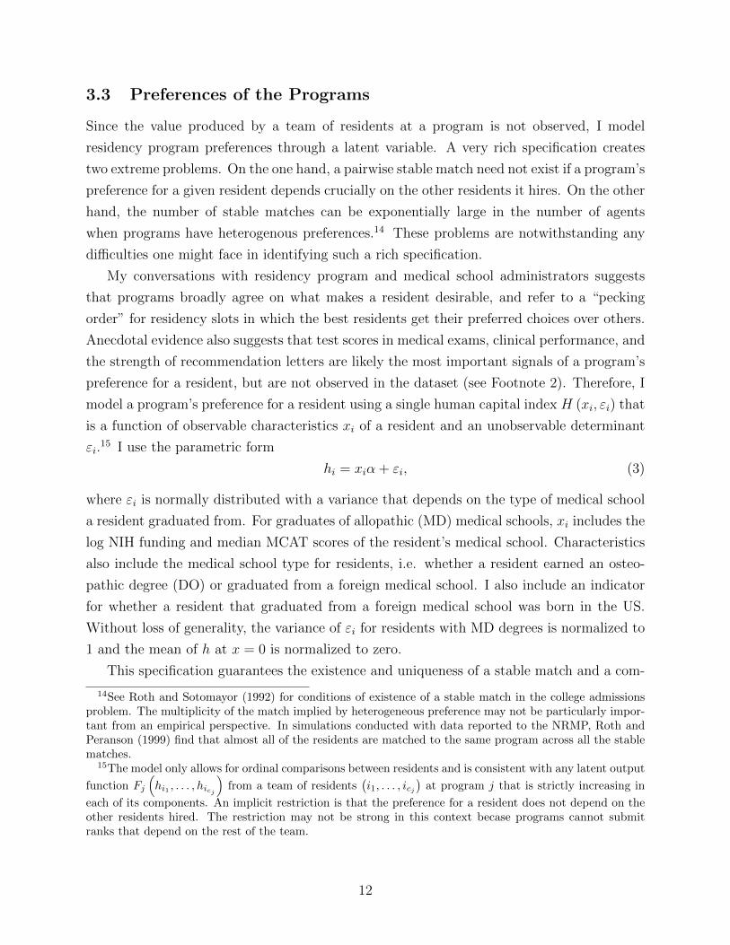
3.3 Preferences of the Programs

Since the value produced by a team of residents at a program is not observed, I model

residency program preferences through a latent variable. A very rich specification creates

two extreme problems. On the one hand, a pairwise stable match need not exist if a program’s

preference for a given resident depends crucially on the other residents it hires. On the other

hand, the number of stable matches can be exponentially large in the number of agents

when programs have heterogenous preferences.14 These problems are notwithstanding any

difficulties one might face in identifying such a rich specification.

My conversations with residency program and medical school administrators suggests

that programs broadly agree on what makes a resident desirable, and refer to a “pecking

order” for residency slots in which the best residents get their preferred choices over others.

Anecdotal evidence also suggests that test scores in medical exams, clinical performance, and

the strength of recommendation letters are likely the most important signals of a program’s

preference for a resident, but are not observed in the dataset (see Footnote 2). Therefore, I

model a program’s preference for a resident using a single human capital index H (xi, εi) that

is a function of observable characteristics xi of a resident and an unobservable determinant

εi.15 I use the parametric form

hi = xiα + εi, (3)

where εi is normally distributed with a variance that depends on the type of medical school

a resident graduated from. For graduates of allopathic (MD) medical schools, xi includes the

log NIH funding and median MCAT scores of the resident’s medical school. Characteristics

also include the medical school type for residents, i.e. whether a resident earned an osteo-

pathic degree (DO) or graduated from a foreign medical school. I also include an indicator

for whether a resident that graduated from a foreign medical school was born in the US.

Without loss of generality, the variance of εi for residents with MD degrees is normalized to

1 and the mean of h at x = 0 is normalized to zero.

This specification guarantees the existence and uniqueness of a stable match and a com-

14See Roth and Sotomayor (1992) for conditions of existence of a stable match in the college admissionsproblem. The multiplicity of the match implied by heterogeneous preference may not be particularly impor-tant from an empirical perspective. In simulations conducted with data reported to the NRMP, Roth andPeranson (1999) find that almost all of the residents are matched to the same program across all the stablematches.

15The model only allows for ordinal comparisons between residents and is consistent with any latent output

function Fj

(hi1 , . . . , hicj

)from a team of residents

(i1, . . . , icj

)at program j that is strictly increasing in

each of its components. An implicit restriction is that the preference for a resident does not depend on theother residents hired. The restriction may not be strong in this context becase programs cannot submitranks that depend on the rest of the team.

12

putationally tractable simulation algorithm that is described in Section 6.3.16 Finally, Sec-

tion 4.3 notes that identifying a model with heterogeneity relies on exclusion restrictions, in

this case an observable program characteristic that is excluded from the preferences of the

residents for programs.

4 Identification

In this section, I describe how the data provide information about preference parameters

using pairwise stability as an assumption on the observed matches. The discussion also

guides the choice of moments used in estimation. Standard revealed preference arguments do

not apply because “choice-sets” of individuals are unobserved and determined in equilibrium.

Instead, I leverage information in the sorting patterns and many-to-one matching to identify

the parameters.

Agarwal and Diamond (2013) study non-parametric identification in a single large market

for a model without heterogenous preferences for programs. They find that having data

from many-to-one matches rather than one-to-one matches is important from an empirical

perspective. A formal treatment of identification is beyond the scope of this paper.

The market index t is omitted in this section because all identification arguments are

based on observing one market with many (interdependent) matches. For simplicity, I also

assume that the number of residents is equal to the number of residency positions and

treat all characteristics as exogenous. Identification of the case with endogenous salaries is

discussed in Section 5, and does not require a reconsideration of arguments presented here.

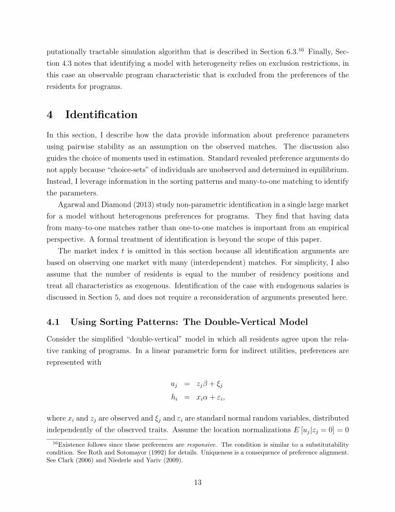
4.1 Using Sorting Patterns: The Double-Vertical Model

Consider the simplified “double-vertical” model in which all residents agree upon the rela-

tive ranking of programs. In a linear parametric form for indirect utilities, preferences are

represented with

uj = zjβ + ξj

hi = xiα + εi,

where xi and zj are observed and ξj and εi are standard normal random variables, distributed

independently of the observed traits. Assume the location normalizations E [uj|zj = 0] = 0

16Existence follows since these preferences are responsive. The condition is similar to a substitutabilitycondition. See Roth and Sotomayor (1992) for details. Uniqueness is a consequence of preference alignment.See Clark (2006) and Niederle and Yariv (2009).

13

and E [hi|xi = 0] = 0.

I begin with an example to show that a sign restriction on one parameter of the model

is needed to interpret sorting patterns in terms of preferences. Consider a model in which x

is a scalar measuring the prestige of a resident’s medical school and z measures the size of

the hospital with which a program is associated. In this example, residents from prestigious

medical schools sort into larger hospitals if the human capital distribution of residents from

more prestigious medical schools is higher and hospital size is preferable. However, this

sorting may also have been observed if residents from prestigious medical schools were less

likely to have high human capital and smaller hospitals were preferable. The observation

necessitates restricting one characteristic of either residents or programs to be desirable.

Throughout the empirical exercises in this paper, I assume that residents graduating from

more prestigious medical schools, as measured by the NIH funding of the medical school, are

more likely to have a higher human capital index.17 Under this sign restriction, the sorting

patterns observed in Figure 1 can only be rationalized if a program’s desirability is positively

related to the NIH funding of its affiliates.

Now I describe how we can compare two sets of observable traits using sorting patterns.

Agarwal and Diamond (2013) generalize the model in this section to allow for non-parametric

functions of x and z, and non-parametric distributions for the additively separable errors ε

and ξ. They prove that sorting patterns can be used to determine if x and x′ (likewise, z

and z′) are equally desirable, but not the distribution of preferences.

To see why we can determine if two observable types are equally desirable, note that the

set of programs with a higher value of zβ have a higher distribution of utility to residents,

and are therefore matched with residents with higher human capital. Using this fact, it

can be shown that if zβ > z′β, the distribution of observable characteristics of residents

matched with programs of type z must be different than that of z′. The sorting observed in

the data thus informs us whether two observable types of programs (analagously residents)

are equally desirable or not. For example, assume that there are two types of programs,

one at larger but less prestigious hospitals than another program at a smaller hospital. The

residents matched with these two hospital types have the same distribution of observable

characteristics only if residents trade-off hospital size for prestige.

4.2 Importance of Data from Many-to-One Matches

The preceding arguments using only sorting patterns do not contain information on the

relative importance of observables on the two sides of the market. For intuition, consider an

17The sign restiction does not imply that all medical students at more prestigous medical schools havehigher human capital index.

14

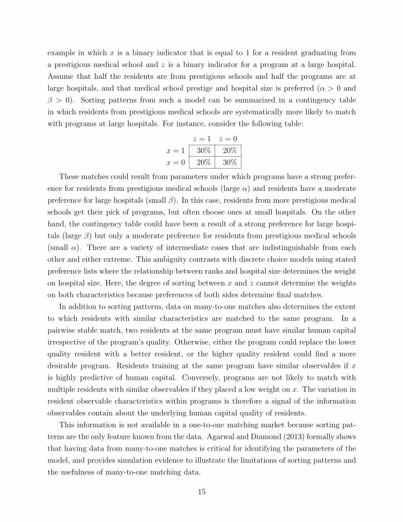
example in which x is a binary indicator that is equal to 1 for a resident graduating from

a prestigious medical school and z is a binary indicator for a program at a large hospital.

Assume that half the residents are from prestigious schools and half the programs are at

large hospitals, and that medical school prestige and hospital size is preferred (α > 0 and

β > 0). Sorting patterns from such a model can be summarized in a contingency table

in which residents from prestigious medical schools are systematically more likely to match

with programs at large hospitals. For instance, consider the following table:

z = 1 z = 0

x = 1 30% 20%

x = 0 20% 30%

These matches could result from parameters under which programs have a strong prefer-

ence for residents from prestigious medical schools (large α) and residents have a moderate

preference for large hospitals (small β). In this case, residents from more prestigious medical

schools get their pick of programs, but often choose ones at small hospitals. On the other

hand, the contingency table could have been a result of a strong preference for large hospi-

tals (large β) but only a moderate preference for residents from prestigious medical schools

(small α). There are a variety of intermediate cases that are indistinguishable from each

other and either extreme. This ambiguity contrasts with discrete choice models using stated

preference lists where the relationship between ranks and hospital size determines the weight

on hospital size. Here, the degree of sorting between x and z cannot determine the weights

on both characteristics because preferences of both sides determine final matches.

In addition to sorting patterns, data on many-to-one matches also determines the extent

to which residents with similar characteristics are matched to the same program. In a

pairwise stable match, two residents at the same program must have similar human capital

irrespective of the program’s quality. Otherwise, either the program could replace the lower

quality resident with a better resident, or the higher quality resident could find a more

desirable program. Residents training at the same program have similar observables if x

is highly predictive of human capital. Conversely, programs are not likely to match with

multiple residents with similar observables if they placed a low weight on x. The variation in

resident observable characteristics within programs is therefore a signal of the information

observables contain about the underlying human capital quality of residents.

This information is not available in a one-to-one matching market because sorting pat-

terns are the only feature known from the data. Agarwal and Diamond (2013) formally shows

that having data from many-to-one matches is critical for identifying the parameters of the

model, and provides simulation evidence to illustrate the limitations of sorting patterns and

the usefulness of many-to-one matching data.

15

4.2.1 Descriptive Statistics from Many-to-One Matching

Table 4 shows the fraction of variation in resident characteristics that is within a program.

Notice that almost none of the variation in the gender of the resident is across programs.

This fact suggests that gender does not determine the human capital of a resident. If gender

were a strong determinant of a resident’s desirability to a program, in a double-vertical

model, one would expect that programs would be systematically male or female dominated.

Summaries of the other characteristics indicate that residents are more systematically sorted

into programs where other residents have more similar qualifications. For instance, about

30% of the variation in the median MCAT score of the residents’ graduating medical schools

decomposes into across program variation. This statistic is higher for the characteristics

foreign medical degree and MD degree.

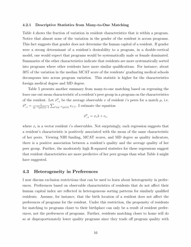
Table 5 presents another summary from many-to-one matching based on regressing the

leave one out mean characteristic of a resident’s peer group in a program on the characteristics

of the resident. Let xµ−i be the average observable x of resident i’s peers for a match µ, i.e.

xµ−i = 1|µ−1(µ(i))|−1

∑i′∈µ−1(µ(i)) xi′,1. I estimate the equation

xµ−i = xiλ+ ei,

where xi is a vector resident i’s observables. Not surprisingly, each regression suggests that

a resident’s characteristic is positively associated with the mean of the same characteristic

of her peers. Viewing NIH funding, MCAT scores, and MD degree as quality indicators,

there is a positive association between a resident’s quality and the average quality of her

peer group. Further, the moderately high R-squared statistics for these regressions suggest

that resident characteristics are more predictive of her peer groups than what Table 4 might

have suggested.

4.3 Heterogeneity in Preferences

I now discuss exclusion restrictions that can be used to learn about heterogeneity in prefer-

ences. Preferences based on observable characteristics of residents that do not affect their

human capital index are reflected in heterogeneous sorting patterns for similarly qualified

residents. Assume, for instance, that the birth location of a resident does not affect the

preferences of programs for the resident. Under this restriction, the propensity of residents

for matching to programs closer to their birthplace can only be a result of resident prefer-

ences, not the preferences of programs. Further, residents matching closer to home will do

so at disproportionately lower quality programs since they trade off program quality with

16

preferences for location.

The principle is similar to the use of variation excluded from one part of a system to

identify a simultaneous equation model. The exclusion restriction in the example above

isolates a factor influencing the demand for residency positions without affecting the distri-

bution of choice sets faced by residents. Conversely, one may use factors that influence the

human capital index of a resident but not their preferences to obtain variation in choice sets

of residents that is independent of resident preferences. Conlon and Mortimer (2010) use a

similar source of variation arising from product availability to identify demand models with

unobserved heterogeneity.

While only one restriction may suffice in theory, the empirical specifications in this pa-

per use both restrictions. Ideally, one would be able to estimate preferences for programs

that are heterogeneous across residents with different medical schools or skill levels. Richer

specifications that allows for this type of preference heterogeneity are difficult to estimate

because quality indicators of residents only include the medical school, and do not vary at

the individual level.

5 Salary Endogeneity

The salary offered by a residency program may be correlated with unobserved program

covariates. For instance, programs with desirable unobserved traits may be able to pay

lower salaries due to compensating differentials. Alternatively, desirable programs may be

more productive or better funded, resulting in salaries that are positively associated with

unobserved quality. One approach to correct for wage endogeneity is to formally model

wage setting. I avoid this for several reasons. First, the allegation of collusive wage setting

in the lawsuit is unresolved. Second, hospitals tend to set identical wages for residents in

all specialties, suggesting that a full model should consider the joint salary setting decision

across all residency programs at a hospital. Finally, a full model would need to account for

accreditation requirements that require salaries to be “adequate” for a resident’s living and

educational expenses.18

5.1 A Control Function Approach

I propose a control function correction for bias due to correlation between salaries wjt and

program unobservables ξjt (see Heckman and Robb, 1985; Blundell and Powell, 2003; Imbens

18The ACGME sponsoring institution requirements state that “Sponsoring and participating sites mustprovide all residents with appropriate financial support and benefits to ensure that they are able to fulfillthe responsibilities of their educational programs.”

17

and Newey, 2009). The principle of the method is similar to that of an instrumental variables

solution to endogeneity. It also relies on an instrument rjt that is excludable from the utility

function U (·). The instrument I use is described in the next section.

Consider the following linear function for the salary wjt offered by program j in period

t :

wjt = zjtγ + rjtτ + νjt, (4)

where zjt are program observable characteristics, rjt is the instrument, and νjt is an unob-

servable. Endogeneity of wjt is captured through correlation between the unobservables νjt

and ξjt. Equation (4) is analogous to the first stage of a two-stage least squares estimator

and the equilibrium model of matches is analogous to the second stage.

The control function approach requires (ξjt, νjt) to be independent of (zjt, rjt). This

assumption replaces weaker conditional moment restriction needed in instrumental variables

approach.19 Under this independence, although wjt is not (unconditionally) independent of

ξjt, it is conditionally independent of ξjt given νjt and zjt. The control function approach

uses a consistent estimate of νjt from the first stage as a conditioning variable in place of its

true value.

Since νjt can be estimated from equation (4) using OLS, treat it as any other observed

characteristic. As noted earlier, we need to allow for correlation between νjt and ξjt to build

endogeneity of wjt into the system. For tractability given the limited salary variation, I

model the distribution of ξjt conditional on νjt as

ξjt = κνjt + σζjt, (5)

where ζjt ∼ N (0, 1) is drawn independently of νjt and (κ, σ) are unknown parameters.

Substitute equation (5) to re-write equation (1) as

uijt = zjtβzi + wjtβ

wi + κνjt + σζjt. (6)

Since variation in wjt given νjt and zjt is due to rjt, the assumptions above imply that ζjt is

independent of wjt, solving the endogeneity problem.

As a scale normalization, I set σ = 1. Note that the unobservable characteristic of the

19Imbens (2007) discusses these independence assumptions at some length, noting that they are commonlymade in the control function literature and are often necessary when dealing with a non-additive second stage.In this context, even though ξjt is additively separable from wjt, the observed matches are not an additivefunction of ξjt and wjt. This fact prohibits the approach used in demand models pioneered by Berry (1994)and Berry et al. (1995), where an inversion can be used to to estimate a variable with a separable form inthe unobserved characteristic and the endogenous variable.

18

program ξjt, may be correlated across time through νjt. For instance, νjt may be the sum of

a random effect νrj that is constant over time for a given j and a per-period deviation νdjt as

long as each of the components is independent of (zjt, rjt).

While it may be possible to relax the linear specification in principle, an important

restriction in this approach is that unobservables of competitor programs cannot affect wages

(except exclusively through νjt). Nonetheless, this linear specification has been shown to

substantially reduce bias in estimates even in models of oligopolistic competition in which

the price has a nonlinear relationship with unobservables and the characteristics of competing

products (Yang et al., 2003; Petrin and Train, 2010).

5.2 Instrument

Table 6 presents regression estimates of equation (5), except using a log-log specification

so that coefficients can be interpreted as elasticities. The first four columns do not include

the instrument rjt, which is defined below. Columns (1) and (2) show limited correlation

between salaries and observed program characteristics except rents and the Medicare wage

index. The elasticity with respect to these two variables is small, at less than 0.15 in magni-

tude. This suggests that models that do not instrument for salaries may provide reasonable

approximations. To address potential correlation, however, I will also present estimates that

use Medicare reimbursement rates for residency training at competitor hospitals as a wage

instrument.

Medicare reimburses residency programs for direct costs of training based on cost reports

submitted in the 1980s. Before the prospective payment system was established, the total

payment made to a hospital did not depend on the precise classification of costs as training

or patient care costs. The reimbursement system for residency training was severed from

payments for patient care in 1985 because the two types of costs were considered distinct

by the government. While patient care was reimbursed based on fees for diagnosis-related

groups, reimbursements for residency training were calculated using cost reports in a base

period, usually 1984. Line items related to salaries and benefits, and administrative expenses

of residency programs were designated as direct costs of residency training. A per resident

amount was calculated by dividing the total reported costs on these line items by the number

of residents in the base period. Today, hospitals are reimbursed based on this per-resident

amount, adjusted for inflation using CPI-U.

This reimbursement system therefore uses reported costs from two decades prior to the

sample period of study. More importantly, the per resident amount may not reflect costs

even in the base period because hospitals had little incentive to account for costs under the

19

correct line item. Newhouse and Wilensky (2001) note that the distinction between patient

care costs from those incurred due to residency training is arbitrary and that variation in

per-resident amounts may be driven by differences in hospital accounting practices rather

than real costs. In other words, whether a cost, say salaries paid to attending physicians,

was accounted for in a line item later designated for direct costs can significantly influence

reimbursement rates today.

These reimbursements are earmarked for costs of residency training and are positively

associated with salaries paid by a program today (Table 6, Column 3). Reimbursement rates

at competitor programs can therefore affect a program’s salary offer because conversations

with program directors suggest that salaries paid by competitors in a program’s geographic

area are used as benchmarks while setting their own salaries (Column 4).20

I instrument using a weighted average of reimbursement rates of other teaching hospitals

in the geographic area of a program. The instrument is defined as

rj =

∑k∈Gj

ftek × rrk∑k∈Gj

ftek, (7)

where rrk and ftek are the reimbursement rate and number of full-time equivalent residents

at program k’s primary hospital in the base period, and Gj are the hospitals in program

j’s geographic area other than j’s primary hospital. I base the geographic definitions on

Medicare’s physician fee schedule, i.e. the MSA of the hospital or the rest of state if the

hospital is not in an MSA. If less than three other competitors are in this area, define Gj to

be the census division.21

Consistent with the theory for the instrument’s effect on salaries, Column (5) shows that

competitor reimbursements are positively related to salaries. Estimated in levels rather than

logs, this specification is analogous to the first stage in a two-stage least-squares method.22

In Column (6), I test the theory that competitor reimbursements affect salaries only through

20Conversations with Dr. Weinstein, Vice President for GME at Partners Healthcare, suggest that salariesat residency programs sponsored by Partners Healthcare are aimed to be competitive with those at otherprograms in the Northeast and in Boston, by looking at market data from two publicly available sources(the COTH Survey and New England/Boston Teaching Hospital Survey).

21Additional details on Medicare’s reimbursement scheme and the construction of the instrument are inAppendix E.

22Figure E.5 in the appendix depicts this first stage visually. A strong increasing relationship betweensalary and competitor reimbursements is noticable. Clustered at the program level, the first stage F-statisticfor the coefficient on the instrument is 37.6. Since the control function approach is based on assumingindependence rather than mean independence, I test for heteroskedasticity in the residuals from the firststage. I could not reject the hypothesis that the residual is homoskedastic at the 90% confidence level forany individual year of data using either the tests proposed by Breusch and Pagan (1979) or by White (1980).Figure E.5 presents a scatter plot of the salary distribution against fitted values. The plot shows littleevidence of heteroskedasticity.

20

competitor salaries. Relative to column (5), controlling for the lagged average competitor

salaries reduces the estimated effect of competitor reimbursements by an order of magnitude

and results in a statistically insignificant effect.

The key assumption for validity of the instrument is that the program unobservable ξjt is

conditionally independent of competitor reimbursement rates, given program characteristics

and a program’s own reimbursement rate, which is included in zjt for specifications using

the instrument. This assumption is satisfied if variation in reimbursement rates is driven

by an arbitrary classification of costs by hospitals in 1984 or if past costs of competitors

are not related to residents’ preferences during the sample period. The primary threat is

that reported per resident costs are correlated with persistent geographic factors. To some

extent, this concern is mitigated by controlling for a program’s own reimbursement rate.

Reassuringly, Column (7) in Table 6 shows that the impact of competitor reimbursement

rates on a program’s salary changes by less than the standard error in the estimates upon

including location characteristics such as median age, household income, crime rates, col-

lege population and total population.23 Another concern is the possibility that programs

respond to the reimbursement rates of competitors by engaging in endogenous investment.

A comparison of estimates from Columns (2) and (5) shows little evidence of sensitivity of

the coefficients on program characteristics (NIH, beds, Case Mix Index) to the inclusion of

reimbursement rate variables.

6 Estimation

This section defines the estimator, the moments used in estimation, the simulation technique

and a parametric bootstrap used for inference.

6.1 Method of Simulated Moments

The estimation proceeds in two stages when the control function is employed. I first estimate

the control variable νjt from equation (4) using OLS to construct the residual

νjt = wjt − zjtγ − rjtτ . (8)

23Strictly speaking, the exclusion restriction requires that the instrument is not strongly correlated withfactors that may determine choices of residents. Appendix E shows that excluded location characteristics donot explain much variation in addition to controls included in the model although a formal test of exogeneitycan be rejected.

21

Replacing this estimate in equation (6), we get

uijt ≈ zijtβzi + wjtβ

wi + κνjt + σζjt, (9)

where the approximation is up to estimation error in νjt. The estimation of parameters de-

termining the human capital index of residents and their preferences over residents proceeds

by treating νjt like any other exogenous observable program characteristic. The error due to

using νjt instead of νjt, however, affects the calculation of standard errors. This first stage

is not necessary in the model treating salaries as exogenous.

The distribution of preferences of residents and human capital can be determined as

a function of observable characteristics of both sides and the parameter of the model, θ

collected from equations (2), (3) and (6). The second stage of the estimation uses a method

of simulated moments estimator (McFadden, 1989; Pakes and Pollard, 1989) to estimate the

true parameter θ0. The estimate θMSM minimizes a simulated criterion function

∥∥m− mS (θ)∥∥2W

=(m− mS (θ)

)′W(m− mS (θ)

),

where m is a set of moments constructed using the matches observed in the sample, mS (θ)

is the average of moments constructed from S simulations of matches in the economy, and

W is a matrix of weights described in Section 6.4. Additional details on the estimator are

in Appendix A.24

6.2 Moments

The vector m consists of sample analogs of three sets of moments, stacked for each market and

then averaged across markets. The simulated counterparts mS (θ) are computed identically,

but averaged across the simulations and markets.

For the match µt observed in market t, the set of moments are given by

1. Moments of the joint distribution of observable characteristics of residents and pro-

grams as given by the matches:

mt,ov =1

Nt

∑i∈Nt

1 {µt (i) = j}xizjt. (10)

24The objective function in the specifications estimated have local minima, and is discontinuous due tothe use of simulation. I use three starts of the genetic algorithm, which is a derivative-free global stochasticoptimization procedure, followed by local searches using the subplex algorithm. Details are in Appendix F.

22

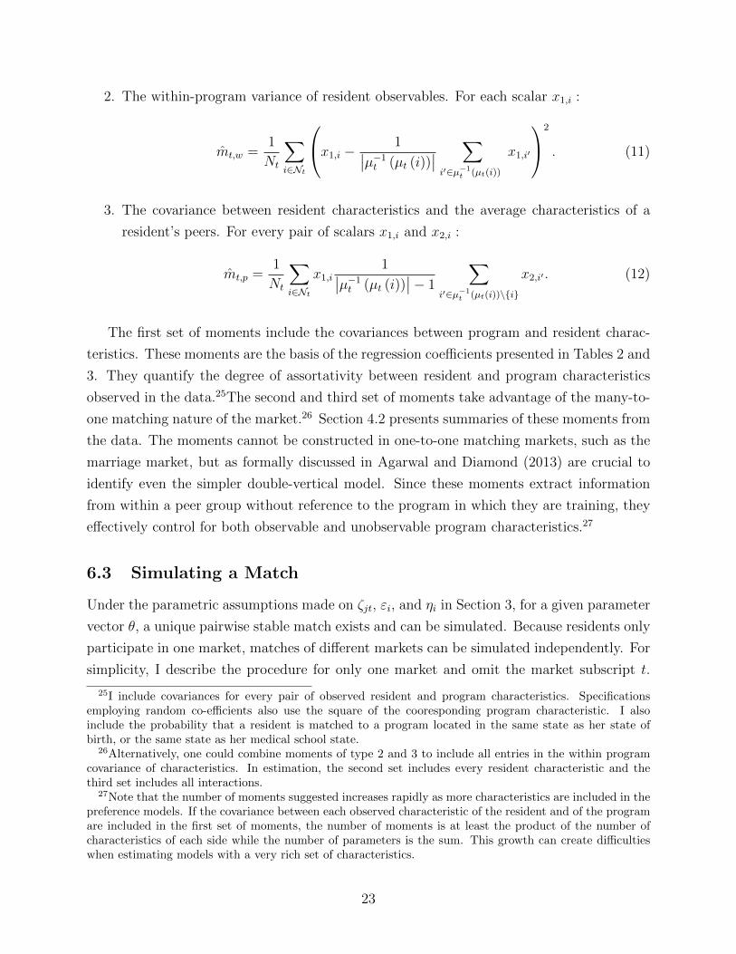
2. The within-program variance of resident observables. For each scalar x1,i :

mt,w =1

Nt

∑i∈Nt

x1,i − 1∣∣µ−1t (µt (i))∣∣ ∑i′∈µ−1

t (µt(i))

x1,i′

2

. (11)

3. The covariance between resident characteristics and the average characteristics of a

resident’s peers. For every pair of scalars x1,i and x2,i :

mt,p =1

Nt

∑i∈Nt

x1,i1∣∣µ−1t (µt (i))

∣∣− 1

∑i′∈µ−1

t (µt(i))\{i}

x2,i′ . (12)

The first set of moments include the covariances between program and resident charac-

teristics. These moments are the basis of the regression coefficients presented in Tables 2 and

3. They quantify the degree of assortativity between resident and program characteristics

observed in the data.25The second and third set of moments take advantage of the many-to-

one matching nature of the market.26 Section 4.2 presents summaries of these moments from

the data. The moments cannot be constructed in one-to-one matching markets, such as the

marriage market, but as formally discussed in Agarwal and Diamond (2013) are crucial to

identify even the simpler double-vertical model. Since these moments extract information

from within a peer group without reference to the program in which they are training, they

effectively control for both observable and unobservable program characteristics.27

6.3 Simulating a Match

Under the parametric assumptions made on ζjt, εi, and ηi in Section 3, for a given parameter

vector θ, a unique pairwise stable match exists and can be simulated. Because residents only

participate in one market, matches of different markets can be simulated independently. For

simplicity, I describe the procedure for only one market and omit the market subscript t.

25I include covariances for every pair of observed resident and program characteristics. Specificationsemploying random co-efficients also use the square of the cooresponding program characteristic. I alsoinclude the probability that a resident is matched to a program located in the same state as her state ofbirth, or the same state as her medical school state.

26Alternatively, one could combine moments of type 2 and 3 to include all entries in the within programcovariance of characteristics. In estimation, the second set includes every resident characteristic and thethird set includes all interactions.

27Note that the number of moments suggested increases rapidly as more characteristics are included in thepreference models. If the covariance between each observed characteristic of the resident and of the programare included in the first set of moments, the number of moments is at least the product of the number ofcharacteristics of each side while the number of parameters is the sum. This growth can create difficultieswhen estimating models with a very rich set of characteristics.

23

For a draw of the unobservables {εis, ηis}Ni=1 and {ζjs}Jj=1 indexed by s, calculate

his = xiα + εis,

and the indirect utilities {uijs}i,j . The indirect utilities determine the program resident i

picks from any choice set.

Begin by sorting the residents in order of their simulated human capital, {his}Ni=1, and

let i(k) be the identity of the resident with the k-th highest human capital.

• Step 1 : Resident i(1) picks her favorite program. Set her simulated match, µs(i(1)), to

this program and compute J (1), the set of programs with unfilled positions after i(1) is

assigned.

• Step k > 1 : Let J (k−1) be the set of programs with unfilled positions after resident

i(k−1) has been assigned. Set µs(i(k))

to the program in J (k−1) most desired by i(k).

The simulated match µs can be used to calculate moments using equations (10) to (12).

The optimization routine keeps a fixed set of simulation draws of unobservable characteristics

for computing moments at different values of θ.

A model with preference heterogeneity on both sides requires a computationally more

complex simulation method, such as the Gale and Shapley (1962) deferred acceptance algo-

rithm (DAA), to compute a particular pairwise stable match. 28

6.4 Econometric Issues

In a data environment with many independent and identically distributed matching markets,

the sample moments and their simulated counterparts across markets can be seen as iid

random variables. Well known limit theorems could be used to understand the asymptotic

properties of a simulation based estimator (McFadden, 1989; Pakes and Pollard, 1989). The

data for this study are taken from eight academic years, making asymptotic approximations

based on data from many markets undesirable. Within each market, the equilibrium match

of agents are interdependent through both observed and unobserved characteristics of other

agents in the market. For this reason, modelling the data generating process as independently

sampled matches is unappealing as well.

28In the DAA, each applicant simultaneously applies to her most favored program that has not yet rejectedher. A set of applications are held at each stage while others are rejected and assignments are made finalonly when no further applications are rejected. This temporary nature of held applications and the needto compute a preferred program for all applications at each stage significantly increases the computationalburden for a market with many participants such as the one studied in this paper.

24

Agarwal and Diamond (2013) consider a data generating process in which the number of

programs and residents increases and each program has two positions. The observed data is a

pairwise stable match forN residents and J programs with characteristics (xi, εi) and (zjt, ξjt)

drawn from their respective population distributions. These large market asymptotics are

appealing in this setting since the family medicine residency market has about 430 programs

and 3,000 residents participating each year. The challenge in obtaining asymptotic theory

arises precisely from the dependence of matches on the entire sample of observed characteris-

tics. They prove that the method of moments estimator is consistent for the double-vertical

model in a single market. They also present Monte Carlo evidence on a simulation based

estimator for a more general model like the one estimated in this. Simulations suggest that

the root mean square error in parameter estimates decreases with the sample size.

Motivated by Agarwal and Diamond (2013), I compute the covariance of the moments is

estimated using a parametric bootstrap 29 to account for the dependence of matches across

residents and approximate the error in the estimated parameter using a delta method that

is commonly used in simulated estimators (Gourieroux and Monfort, 1997):

Σ =(

Γ′W Γ)−1

Γ′W

(V +

1

SV S

)W ′Γ

(Γ′W Γ

)−1,

where Γ is the gradient of the moments with respect to θ evaluated at θMSM using two-sided

finite-difference derivatives; W is the weight matrix used in estimation; V is an estimate of

the covariance of the moments at θMSM ; S is the number of simulations and V S is an estimate

of the simulation error in the moments at θMSM .

I now describe the choice of W and outline the parametric bootstrap used to estimate V

for the simpler case where the number of residents is equal to the total number of resident

positions and salaries are exogenous. Appendix A provides additional details on estimating

Σ. The bootstrap mimics the data generating process in which a pairwise stable match

between random sample of residents and programs is observed. Three basic steps are used

for each bootstrap iteration b ∈ {1, . . . , B} :

1. Generate a bootstrap sample of programs {zj,b, cj,b}Jj=1 by drawing from the empirical

distribution FZ,C with replacement. Calculate Ctot,b =∑

j cj,b.

2. Generate a bootstrap sample of residents {xi,b}Ctot,b

i=1 from FX , with replacement.

29Agarwal and Diamond (2013) use a parametric bootstrap for the estimator in their Monte Carlo ex-periments. However, with the higher dimensional parameter space, bootstrapping the estimator directly iscomputationally prohibitive.

25

3. Simulate the unobservables (εi,b, ηi,b, ξjt,b) to compute {hi,b}Ctot,b

b=1 and {ui,j,b}i,j at θMSM .

Calculate the stable match µb for bootstrap b and corresponding moments mb.

The variance of mb is the estimate for V used to compute Σ. Monte Carlo evidence

suggests that the procedure yields confidence sets with close to the correct size. The model

using the control function correction has an additional step in this bootstrap to account for

uncertainty in estimating νjt, also described in Appendix A.1.

Finally, the weight matrix in estimation is obtained from bootstrapping directly from

the distribution of matches observed in the data. A bootstrap sample of matches {µb}Bb=1

is generated by sampling, with replacement, J programs and along with their matched

residents. The moments from these matches are computed and the inverse of the covariance

is used as the positive definite weight matrix, W . The procedure does not require a first step

optimization and has other advantages discussed in Appendix A.2.

7 Empirical Specifications and Results

I present estimates from three models. The first model has the richest form of preferences as

it allows for unobserved heterogeneity in preferences for diagnostic mix, research focus and

hospital size via normally distributed random coefficients on Case Mix Index, NIH Funds of

major medical school affiliates and the number of beds. It also allows for heterogeneity in

taste for program location based on a resident’s birth location and medical school location. I

use a second model that does not include random coefficients on Case Mix, NIH Funds or beds

to assess the importance of unobserved preference heterogeneity. These two models treat

salaries as exogenous. The final model modifies the second model to addresses the potential

endogeneity in salaries using the instrument described in Section 5.2. This specification

includes a program’s own reimbursement rate in addition to characteristics included in the

other models.

Estimates of residents’ preferences for programs presented in the next section are trans-

lated into dollar equivalents for a select set of program characteristics. I also present the

willingness to pay by categories of programs. These are the most economically relevant

statistics obtained from preference estimates. Appendix C briefly discusses the underly-

ing parameters, which are not economically intuitive, and robustness using estimates from

additional models.

26

7.1 Preference Estimates

Panel A.1 of Table 7 presents the estimated preferences for programs in salary equivalent

terms. Comparing specifications (1) and (2), the estimated value of a one standard deviation

higher Case Mix Index at an otherwise identical program is about $2,500 to $5,000 in annual

salary for a typical resident. Likewise, residents are willing to pay for programs at larger

hospitals as measured by beds, and for programs with better NIH funded affiliates. The

estimates from specification (1) suggest a substantial degree of preference heterogeneity

for these characteristics as well. The additional heterogeneity in preferences relative to

specification (2) results in a shift in the mean willingness to pay for NIH funding of major

affiliates, the Case Mix Index, and beds, but not whether they are desirable or not.

Panel A.2 presents estimates of preferences for program types and heterogeneity in pref-

erences for program location. Both specifications (1) and (2) estimate that, ceteris paribus,

rural programs are preferable to urban programs. However, the next section, which presents

residents’ willingness to pay by program categories, shows that the typical rural programs is

less preferred to urban programs because rural programs tend to be associated with smaller

hospitals and medical school affiliates with lower NIH funding.

Estimates from both specifications also suggest that residents prefer programs in their

state of birth or in the same state as their medical school. For instance, estimates from

specification (1) imply that a typical resident is willing to forgo about $10,000 in salary to

match at a program in the same state as their medical school. Although rural born residents

prefer rural programs more than other residents, they prefer rural programs at a monetary

equivalent of under $1,200. The estimated willingness to pay for these factors is smaller in

specification (2) although the relative importance for the different dimensions is similar.

Panel B presents parameter estimates for the distribution of human capital, which deter-

mines ordinal rankings between residents. All specifications yield similar coefficients on the

various resident characteristics and estimate that the unobservable determinants of human

capital have larger variances for residents with foreign degrees. The estimated difference

between a US born foreign medical graduate and foreign graduates from other countries is

an order of magnitude smaller than the standard deviation of unobservable determinants of

human capital.

7.1.1 Estimates usign Wage Instruments

As compared to estimates from specification (2), which treats salaries as exogenous, the

estimated willingness to pay for program characteristics is generally larger in specification

(3). The estimates for NIH funding of Major Medical school affiliates is the only exception.

27

The increase in the estimated willingness to pay in specification (3) is driven by a fall in the

coefficient on salaries but similar coefficient estimates for the other program characteristics.

Appendix C discusses results from the instrumented version of specification (1), which also

leads to a decrease in the coefficient on salaries and little change in estimates for other

coefficients. This specification results in a small, positive coefficient on salaries that is

not statistically significant and implies an implausibly large willingness to pay for better

programs.

The qualitative effect of including the wage instrument on parameter estimates indicates

that, if anything, treating salaries as exogenous may lead to an understated willingness to

pay for more desirable programs. I interpret the magnitudes with caution given the lack of

robustness, which is likely a consequence of the limited salary variation in the data.30 Aside

for controlled geographic covariates such as rent and wage index, estimates in Column (2)

of Table 6 do not show strong evidence of substantial correlation of salaries with program

characteristics. My preferred approach is to focus on results from specification (1) for most

counterfactual results and discuss the effect of possible positive bias in the salary coefficient

using specification (3).

7.1.2 Distribution of Willingness to Pay

The distribution of willingness to pay for different programs is an important economic input

for analyzing salaries under competitive wage bargaining. Table 8 presents summary statis-

tics of this distribution by categorizing programs into quartiles based on observed character-

istics, and normalizing the mean across all programs to zero. I estimate a large willingness to

pay for programs with a high Case Mix Index, at larger hospitals and in counties with higher

rent. A typical resident is willing to accept a $5,000 to $9,500 lower salary at the average

urban program instead of a training in a rural location. Specifications (1) and (2) estimate

the standard deviation in utility across residents and programs of varying characteristics to

be between $14,000 and $22,000. This measure doubles from $14,000, but is imprecisely

estimated, when Specification (2) is modified to account for endogeneity in salaries. The

large willingess to pay for more desirable programs may arise from differences in the value

added by programs as well as contemporaneous value for desirable amenities, such as tastes

for geographically nearby programs.

30The objective function for specifications using salary instruments is fairly flat along different combina-tions of coefficients on the wage and control variable.

28

7.2 Model Fit

In this section, I describe the in-sample and out-of-sample fit of estimates from specification

(1). The fit of specifications (2) and (3) are qualitatively similar. The out-of-sample fit uses

data from the 2011-2012 wave of the GME Census, which was only accessed after parameter

estimates were computed.

Estimates of the model only determine the probability that a resident with a given

observable characteristic matches with a program with certain observables. The uncertainty

in matches arises from unobservables of both the residents and the programs. Therefore,

an assessment of fit must use statistics that average matches across groups of residents or

programs.

For simplicity, I assess model fit using a single dimensional average quality of matched

program for a group of residents with similar observable determinants of human capital. I

use the parameter estimates from the model to construct a quality index for each resident

i and program j by computing xiα and zjtβ respectively. For each year t, I then divide

the residents into ten bins based on xiα and compute the mean quality of program with

which residents from each bin are matched. Figure 2 presents a binned scatter plot of this

mean quality of program as observed in the data and predicated by model simulations.

Both the in-sample points and the out-of-sample points are close to the 45-degree line. The

90% confidence sets of the simulated means for several resident bins include the theoretical

prediction.31

This fit of the model provides confidence that parametric restrictions on the model are

not leading to poor predictions of the sorting patterns in the market. Therefore, I am

comfortable using estimates as basis of counterfactual analysis.

8 Salary Competition

In 2002, a group of former residents brought on a class-action lawsuit under the Sherman Act

against major medical associations in the United States and the NRMP. The plaintiffs alleged

the medical match is an instrumental competitive restraint used by the residency programs

to depress salaries.32 By replacing a traditional market in which residents could use multiple

31A more model-free assessment of fit using sorting regressions only on observed covariates is presentedin Table C.2. One may also worry predicting sorting patterns is is mechanical because there is little changein the market composition across years. For counterfactuals directly impacting the composition of marketparticipants, it can be important for the model to capture changes in sorting as a function of changes in thecomposition of the market. However, changes in the composition of the resident and program distributionare negligible, resulting in little available variation to test the model with such a fit.

32Jung et.al. v AAMC et.al. (2002) states that “The NRMP matching program has the purpose andeffect of depressing, standardizing and stabilizing compensation and other terms of employment.” After the

29

offers to negotiate with programs, they argued that the NRMP “enabled employers to obtain

resident physicians without such a bidding war, thereby artificially fixing, depressing, stan-

dardizing and stabilizing compensation and other terms of employment below competitive

levels” (Jung et.al. v AAMC et.al., 2002). A brief prepared by Orley Ashenfelter on behalf

of the plaintiffs argued that competitive outcomes in this market would yield wages close to

the marginal product of labor, which was approximated using salaries of starting physicians,

nurse practitioners, and physician assistants.33 Physician assistants earned a median salary

of $86,000 in 201034 as compared to about $47,000 for medical residents despite longer work

hours.35

Recent research has debated whether low salaries observed in this market are a results

of the match. Using a stylized model, Bulow and Levin (2006) argue that salaries may be

depressed in the match because residency programs face the risk that a higher salary may

not necessarily result in a better resident. Kojima (2007) uses an example to show that this

result is not robust in a many-to-one matching setting because of cross-subsidization across

residents in a program. Empirical evidence in Niederle and Roth (2003, 2009) suggests that

medical fellowship salaries are not affected by the presence of a match, however, the study

does not explain why fellowship salaries remain lower than salaries paid to other health

professionals.

The plaintiffs argued their case based on a classical economic model of homogeneous

firms competing for the services of labor and free entry. However, such a perfect competition

benchmark may not be a good approximation for an entry-level professional labor market.

The data provide strong evidence that residents have preferences for characteristics of the

program other than the wages and may, thus, reject a higher salary offer from a less desirable

program. Further, barriers to entry by residency programs are high and capacity constraints

are imposed by accreditation requirements. A program must therefore consider the option

value of hiring a substitute resident when confronted with a competing salary offer. High

quality programs may be particularly able to find other residents willing to work for low

salaries. Conversely, highly skilled residents are scarce and they may be able to bargain for

higher salaries. It is essential to consider these incentives in order to predict outcomes under

competitive salary bargaining.

lawsuit was filed, the Pension Funding and Equity Act of 2004 amended antitrust law to disallow evidence ofparticipation in the medical match in antitrust cases. The lawsuit was dismissed following this amendment,overturning a previous opinion of the court upholding the price-fixing allegation.

33A redacted copy of the expert report submitted on behalf of the plaintiffs is available on request.34Source: Bureau of Labor Studies.35At 50 work-weeks a year and 80 hour a week, the cap imposed by the ACGME in 2003, a salary of

$50,000 yields a wage rate for a medical resident of $12.50. A more generous estimate with 65 hours a week,45 work-weeks a year and a salary of $60,000 yields a wage rate of $20.50.

30

I model a “traditional” market using a competitive equilibrium, which is described by

a vector of worker-firm specific salaries and an assignment such that each worker and firm

demands precisely the prescribed assignment. Shapley and Shubik (1971) show that compet-

itive equilibria correspond to core allocations and satisfy two conditions. First, allocations

must be individually rational for both workers and firms. Second, it must be that at the

going salaries no worker-firm pair would prefer to break the allocation to form a (different)

match at renegotiated salaries. This latter requirement ensures that further negotiations

cannot be mutually beneficial. Kelso and Crawford (1982) show that competitive equilibria

can result from a salary adjustment process in which the salaries of residents with multiple

offers are sequentially increased until the market clears. The process embodies the “bid-

ding war” plaintiffs suggest would arise in a “traditional” market. In fact, Crawford (2008)

proposed a redesign of the residency match based on the salary adjustment process with

the aim of increasing the flexibility of salaries in the residency market and implementing a

competitive equilibrium outcome.

I first develop a stylized model to derive the dependence of competitive equilibrium

salaries on both the willingness to pay for programs and the production technology of res-

idency programs. For counterfactual simulations, I adopt an approach that does not rely

on knowing the production technology of resident-program pairs because data on residency

program output is not available. Instead of calculating equilibrium salaries, I use the esti-

mates of only the residents’ preferences to calculate an equilibrium markdown from output

net of training costs, called the implicit tuition. Loosely speaking, my calculation acts as

if the output produced by a program-resident pair accrues entirely to residents. The illus-

trative model shows that the approach is likely to understate the equilibrium markdown in

salaries since programs do not earn any infra-marginal productive rents due to their own

productivity. The theoretical model is also used to describe differences with related models

of on-the-job training or salary setting with non-pecuniary amenities.

8.1 An Illustrative Assignment Model

I generalize the model of the residency market in Bulow and Levin (2006) which assumes that

residents take the highest salary offer. I allow resident preferences to depend on program

quality in addition to salaries, and use a more flexible production function than Bulow and

Levin (2006).

Consider an economy with N residents and programs in which each program may hire

only one resident. Resident i has a human capital index, hi ∈ [0,∞), and program j has a

quality of training index, qj ∈ [0,∞). To focus on salary bargaining, the training quality of

31

programs are held exogenous. Without loss of generality, index the residents and programs

so that hi ≥ hi−1, qj ≥ qj−1, and normalize q1 and h1 to zero.

Residents have homogenous, quasi-linear preferences for the quality of program, u (q, w) =

aq + w with a ≥ 0. The value, net of variable training costs, to a program of quality q of

employing a resident with human capital index h is f (h, q) where fh, fq, fhq > 0 and f (0, 0)

is normalized to 0.36 A program’s profit from hiring resident h at salary level w is f (h, q)−w.

I assume that an allocation is individually rational for a resident if u (q, w) ≥ 0, and for a

program if f (h, q)− w ≥ 0.

A competitive equilibrium assignment maximizes total surplus. In this model, the unique

equilibrium is characterized by positive assortative matching and full employment. Hence,

in equilibrium, resident k is matched with program k and is paid a possibly negative wage

wk. The vector of equilibrium wages is determined by the individual rationality constraints

and the constraint

f (hk, qk)− wk ≥ f (hi, qk)− wi + a (qk − qi) .

This constraint on wk requires that the profit of program k by hiring resident k must be

weakly greater than the profit from hiring resident i. At the going salaries, it is incentive

compatible for resident i to accept an offer from program k only if the wage is at least

wi − a (qk − qi).There is a range of wages that are a part of a competitive equilibrium. Shapley and

Shubik (1971) shows that there exists an equilibrium that is weakly preferred by all resi-

dents to all other equilibria, and another that is preferred by all programs. Appendix B.1

characterizes the entire set of equilibria, and derives the expression for wages at these two

extremal outcomes. Since the plaintiffs alleged that salaries are currently much lower than

in a bargaining process, I focus on the worker-optimal equilibrium which has higher salaries

for every worker than any other equilibrium. This outcome is unanimously preferred by

all residents to other competitive equilibria. The wage of resident k in the worker optimal

equilibrium is given by

wk = −aqk +k∑i=2

[f (hi, qi)− f (hi−1, qi)] . (13)

Resident 1 receives her product of labor f (h1, q1) (normalized to 0), the maximum her

employer is willing to pay. For resident 2, the first term aq2 represents an implicit price

for the difference in the value of training received by her compared to that of program 1

36A complementary production technology is commonly assumed for studying on-the-job training (Becker,1975, pp 34) or sorting in matching markets (Becker, 1973).

32

(with q1 = 0). If a resident were to use a wage offer of w by program 1 in a negotiation

with program 2, the resident would accept a counter offer of w − aq2. The second term in

this resident’s wage, f (h2, q2) − f (h1, q2), is program 2’s maximum willingness to pay for

the difference in productivity of residents 1 and 2, which accrues entirely to the resident in

the worker-optimal equilibrium. The sum of these two terms measures the impact of the

outside option of each party on the wage negotiation determining w2. For k > 2, these

(local) differences in the productivity of residents add up across lower matches to form the

equilibrium wage.

8.2 Implicit Tuition

The implicit price for training at firm k, given by aqk, is based on the preferences for training

at a program rather than the cost of training. In models of general training that use a perfect

competition framework, such as Rosen (1972) and Becker (1975), the implicit price is the

marginal cost of training alone because free entry prevents firms from earning rents due

to their quality.37 When entry barriers are large due to fixed costs or restrictions from

accreditation requirements, firms can earn additional profits due to their quality. I argue

that ruling out entry is appropriate because of accreditation requirements and to focus

on wage bargaining. Equation (13) shows that under these assumptions, program k can

levy the implicit tuition aqk on residents. This implicit tuition results from a force similar

to compensating differentials (Rosen, 1987), but allows for heterogeneity in resident skill.

Equilibrium salaries are the sum of the implicit tuition and a split of the value f produced

by a resident program pair.

As mentioned earlier, the data does not allow us to determine f . I calculate the implicit

tuition using residents’ preferences alone in order to evaluate whether a gap between f and

equilibrium salaries exists as a result of market fundamentals. The next result shows that

the implicit tuition bounds the markdown in salaries from below. Under free entry by firms,

salaries would be equal to f because any profits earned by firms would be competed away.

Proposition 1 For all production functions f with fh, fq, fhq ≥ 0, the profits of the firm

k is bounded below by the implicit tuition, aqk, in any competitive equilibrium.

37Viewing f (h, q) as output net of costs of training, a constant training cost across residents and programswould shift the wage schedule down by that constant. As can be seen from equation (13), training costs thatdepend on program quality, but not the quality of the resident do not affect equilibrium salaries as long asfq remains positive. Also note that the implicit price aqk does not depend on the number of residents andprograms N , which could be very large, or the distribution of program quality. Intuitively, the importantdifference overturning results from perfect competition is that the number of firms competing for a fixed setof workers is not disproportionately large.

33

Proof. Corollary to Proposition 5 stated and proved in Appendix B.2.

Hence, the implicit tuition aqk is a markdown in salaries that is independent of the

output. If residents have a strong preference for program quality, this implicit tuition will

be large and salaries in any competitive equilibrium are well below the product f (hk, qk).

To interpret the implicit tuition as a lower bound for salary markdowns, consider two

particular limiting cases for the production function. If f (h, q) depends only on h so that

the value of a resident, denoted f (h), does not vary across programs, the worker-optimal

salaries are given by

wk = f (hk)− aqk. (14)

Under this production function, the resident is the full claimant of the value of her labor and

salaries equal her product net of the implicit tuition. Residents are able to engage programs

in a bidding war until their salary equals the output less the implicit tuition because all

programs value resident k at f (hk).

On the other hand, if f (h, q) depends only on q so that all residents produce f (q),

irrespective of their human capital, the worker-optimal salaries are

wk = −aqk. (15)

In this case, the program does not share the product f (qk) with the resident since any two

residents are equally productive at the program. The resident still pays an implicit tuition

for training.38

The production function directly influences competitive salaries but Proposition 1 shows

that in all cases resident k pays the implicit tuition aqk. Equilibrium wages given in equa-

tions (14) and (15) highlight that the side of the market that owns the factor determining

differences in f is compensated for their productivity in a competitive equilibrium. Residents

are compensated for their skill only if human capital is an important determinant of f . For

this reason, using a production function of the form f (h) results in a markdown in salaries

from f that is only due to the implicit tuition.

This interpretation highlights a key difference from results derived using models with

many firms competing for labor with free entry. In those models, one expects all the product

to accrue to the workers because firms enter the market to bid for labor services until a zero

profit condition is met. High compensation for residents is a result of free entry rather than

negotiations between a fixed set of agents.

38In order to ensure that the match is assortative in these limiting cases, I assume that if a program(resident) has two equally attractive offers, the tie in favor of the resident (program) with the higher humancapital (quality).

34

8.3 Generalizing the Implicit Tuition

The expression for the implicit tuition derived above relied on the assumption that residents

have homogeneous preferences for program quality. For this reason, the results from the

illustrative model do not speak to competitive outcomes in a model with heterogenous pref-

erences. This section generalizes the definition of implicit tuition to make it applicable to

the model defined in Section 3.

Notice that the profit earned by program k in a worker-optimal equilibrium under a pro-

duction function of the form f (h) is precisely the implicit tuition aqk because this production

function does not provide programs with infra-marginal productive rents. Under this pro-

duction function, markdowns from output are determined only by residents’ preferences for

programs. Consequently, calculating firm profits using a production function of this type

may provide a conservative approach to estimating payoffs to programs more generally. The

next result shows that under heterogeneous preferences for programs, the difference between

salaries and output is the same for all production functions of the form f (h). This ensures

that an implicit tuition can be defined and calculated using only the residents’ willingness

to pay for programs, circumventing the need for estimating f .

For notational simplicity, I state the result for a one-to-one assignment model, and the

general result for many-to-one setting is stated and proved in Appendix B.3.39 With a slight

abuse of notation, let the total surplus from the pair (i, j) be 0.40 Here, uij is the utility,

net of wages, that resident i receives from matching with program j and f (hi) is the output

produced by resident i. I now characterize the equilibria for a modified assignment game in

which the surplus produced by the pair is afij = uij + f (hi) ≥ 0 in terms of the equilibria of

the game with surplus afij.

Proposition 2 The equilibrium assignments of the games defined by afij and afij coincide.

Further, if ufi and vfj are equilibrium payoffs for the surplus afij, then ufi = ufi + f (hi)−f (hi)

and vfj = vfj are equilibrium payoffs under the surplus afij. Hence, a firm’s profit in a worker-

optimal equilibrium depends on {uij}i,j but is identical for all production functions of the form

f (h).

Proof. See Appendix B.3 for the general case with many-to-one matches.

As in the illustrative model, under a production technology that depends only on human

capital, the residents are the residual claimants of output. An increase or decrease in the

39In the general formulation, I assume that the total output from a team of residents(h1, . . . , hqj

)is

F(h1, . . . , hqj

)=∑qj

k=1 f (hk), where f (hk) = 0 if position k is not filled.40This formulation implicitly assumes that, at every program, it is individually rational for a worker to

accept a salary equal to her product. It further assumes that the output of every resident is non-negative.

35

productivity of human capital is reflected in the wages, one for one. The firms’ profits de-

pends only on the preferences of the residents. Thus, I refer to the difference between output

and salaries in the worker-optimal competitive equilibrium for a model in which f depends

only on h as the implicit tuition. This definition uses the assumption that preferences of the

programs can be represented using a single human capital index in the empirical model but

also makes the additional restriction that the productivity of human capital, in dollar terms,

does not depend on the identity of the program.

To the best of my knowledge, a closed form expression for competitive equilibrium salaries

is not available when preferences of the residents are heterogeneous. I calculate the implicit

tuition implied by estimated preferences using a two-step procedure.41 Each step solves a

linear program based on the approach developed in Shapley and Shubik (1971):

• Step 1 : Solve the optimal assignment problem, modified from the formulation by

Shapley and Shubik (1971) to allow for many-to-one matching.

• Step 2 : Calculate the worker-optimal element in the core given the assignments from

step 1.

Appendix B.4 describes the procedure in more detail. All calculations are done with the

2010-2011 sample of the data.

8.4 Estimates of Implicit Tuition

Estimates presented in Section 7 suggest that residents are willing to take large salary cuts in

order to train at more preferred programs, which can translate into a large implicit tuitions.

Table 9 presents summary statistics of the distribution of implicit tuition using estimates

from specifications (1) through (3). I estimate the average implicit tuition to be about

$23,000 for specifications (1) and (2). This estimate rises to $43,500 when using the instru-

ment in specification (3) because the coefficient on salaries falls. As mentioned in Section

7, the instrument used appears weak and yields non-robust point estimates, but generally

results in a larger willingness to pay and implicit tuitions through a decrease in the coeffi-

cient on salaries.42 The standard error in the estimate using specification (3) is also large, at

41Since the total number of residents observed in the market is less than the number of positions and thevalue of options outside the residency market are difficult to determine, I will assume that the equilibriumis characterized by full employment. This property follows if, for instance, it is individually rational forall residents to be matched with their least desirable program at a wage that is equal to the total productproduced by the resident at this program and the product produced by a resident is not negative.

42The instrumented version of specification (1) results in implicit tuition estimates much larger than theones reported because of the smaller estimated coefficient on salaries.

36

$13,700, but can rule out an average implicit tuition smaller than $17,000. These estimates

are economically large in comparison to the mean salary of about $47,000 paid to residents.

The results also show significant dispersion in the implicit tuition across residents and

programs. The standard deviation in the implicit tuition is between $12,000 and $25,000.

The 75th percentile of implicit tuition can be about three times higher than the 25th per-

centile, with even higher values at the 95th percentile. This dispersion primarily arises from

the differences in program quality, which allows higher quality programs to lower salaries

more than relatively lower quality program.

The estimated implicit tuition is between 50% to 100% of the $40,000 salary difference

between medical residents and physician assistants. This finding refutes the plaintiffs’ ar-

gument that the salary gap would not exist if residents’ salaries were set competitively and

physician assistant salaries approximated the productivity of residents. However, the esti-

mated implicit tuition cannot explain the salary gap between starting physicians and medical

residents, which is approximately $90,000.43 As discussed earlier, the implicit tuition is a

conservative estimate of the salary markdown and part of this salary gap may be due to

differences in the productivity of medical residents and starting physicians.

When residents’ preferences are heterogeneous, the implicit tuition is also a function of

the relative demand and supply of different types of residency positions, and is not simply

a result of compensating differentials. Estimates from specification (1) imply a willingness

to pay by residents for programs in the same state as their medical school, and programs in

the same state as their birth state. Therefore, the demand for residency positions is high

in states where many residents were born or states where many residents went to medical

school. A supply-demand imbalance occurs, for instance, when the number of residency

positions in the state is low but many residents have preference for training in that state.

These forces will be important determinants of equilibrium salary if the residency market

adopts the design proposed in Crawford (2008) because the proposal is intended to produce

a competitive equilibrium outcome.

To demonstrate the effect of this imbalance on the estimated implicit tuition, I present

results from the regression

ln yj = zjρ1 + ρ2 lnnpossj + ρ3 ln grsj + ρ4 ln bornsj + ej,

where yj is the average implicit tuition at program j estimated using specification (1), zj

are characteristics of program j included in specification (1), sj is program j’s state, npossj

43I use Mincer equation estimated using interval regressions on confidential data from the Health PhysicianTracking Survey of 2008 to calculate the average salaries for starting family physicians. Details available onrequest.

37

is the number of residency positions offered in sj, grsj is the number of residents from MD

medical schools in state sj and bornsj is the number of residents born in state sj. Column

(4) of Table 10 shows that the elasticity of the average implicit tuition at a program with

respect to the number of family medicine graduates getting their degrees in a medical school

in that state is positive, ρ3 = 0.19. Conversely, the elasticity with respect to the number of

positions offered in the program’s state is negative, ρ2 = −0.16 . The estimate for ρ4 is not

statistically significant, partially because the estimated preference for birth state is low and

because supply-demand imbalance based on birth-state is also lower.

9 Conclusion

Two key features of two-sided matching markets are that agents are heterogeneous and that

highly individualized prices are often not used. Both properties have important implica-

tions for equilibrium outcomes, especially when barriers to entry are substantial, because

assignments are determined by the mutual choices of agents rather than price-based market

clearing. A quantitative analysis of counterfactual market structures may therefore require

estimates of preferences on both sides of the market.

When data on stated preferences is available, extensions of discrete choice methods can

provide straightforward techniques for analysis (see Hastings et al., 2009; Agarwal et al., 2013,

among others). A common constraint is that only data on employer-employee matches or

student enrollment records, rather than stated preferences, are available. This paper develops

empirical methods for recovering preferences of agents in two-sided markets with low frictions

using only data on final matches. I use pairwise stability together with a vertical preference

restriction on one side of the market to estimate preference parameters using the method of

simulated moments. The empirical strategy is based on using sorting patterns observed in

the data and information available only in many-to-one matching. Sorting patterns alone

cannot be used identify the parameters of even a highly simplified model with homogeneous

preferences on both sides of the market.

These methods allow me to quantitatively analyze whether centralization in this market is

the cause of low salaries. I find that heterogeneity in program types and capacity constraints

result in quantitatively large departures from the perfect competition model suggested by

the plaintiffs in the lawsuit. Theoretical results presented in Section 8 show that equilibrium

salaries can be well below the product of labor, net of costs of training, when residents

value the quality of a program. Counterfactual estimates show that the willingness to pay

for programs results in salary markdowns (implicit tuition) between $23,000 and $43,000

in any competitive wage equilibrium. The upper end of estimates can explain the salary

38

gap between physician assistants and medical residents assuming that physician assistant

salaries are close to the productivity of residents. My estimates also show that higher quality

programs would earn a larger implicit tuition than less desirable programs. To the extent that

higher quality programs are matched with higher skilled residents and are also instrinsically

more productive, the implicit tuition is a countervailing force to high dispersion salaries

driven by productivity differences. The implicit tuition may therefore explain the empirical

observations of Niederle and Roth (2003, 2009) in fellowship markets.

The result suggests that the limited supply of heterogeneous residency positions, due to

barriers to entry or accreditation requirements, is the primary cause of low salaries, and

weighs against the view the match is responsible for low resident salaries. In this market,

salaries may also be influenced by the previously mentioned guideline requiring minimum

financial compensations for residents. While these forces may be important, they seem

unrelated to the match. In other words, programs may not have the incentive to pay salaries

close to levels suggested by the plaintiffs because of economic primitives.

The methods and analysis in this paper can be extended in several directions. The re-

striction on the preferences of one side of the market could be relaxed in other markets if

the data contain information that would allow estimating heterogeneous preferences on both

sides of the market. For instance, it may have been possible to estimate heterogenous pref-

erences for residents if program characteristics that can plausibly be excluded from resident

preferences were observed. Future research in other matching markets could use data from

several markets in which the composition of market participants differs in order to estimate

heterogeneous preferences on both sides. These extensions must also confront methodological

hurdles arising from a multiplicity of equilibria are important in other matching markets.

References

Agarwal, N., Abdulkadiroglu, A., and Pathak, P. A. (2013). Sorting and Welfare Conse-quences of Coordinated Admissions: Evidence from New York City.

Agarwal, N. and Diamond, W. F. (2013). Identification and Estimation in Two-sided Match-ing Markets.

Akkus, O., Cookson, A., and Hortacsu, A. (2012). The Determinants of Bank Mergers: ARevealed Preference Analysis.

Bajari, P. and Fox, J. T. (2005). Measuring the Efficiency of an FCC Spectrum Auction.

Becker, G. S. (1973). A Theory of Marriage: Part I. Journal of Political Economy, 81(4):813– 46.

Becker, G. S. (1975). Human Capital: A Theoretical and Empirical Analysis, with SpecialReference to Education, 2nd ed. National Bureau of Economic Research, Inc, New York.

39

Berry, S. T. (1994). Estimating Discrete-Choice Models of Product Differentiation. RANDJournal of Economics, 25(2):242 – 262.

Berry, S. T., Levinsohn, J., and Pakes, A. (1995). Automobile Prices in Market Equilibrium.Econometrica, 63(4):841 – 890.

Berry, S. T. and Pakes, A. (2007). The Pure Characteristics Demand Model. InternationalEconomic Review, 48(4):1193–1225.

Blundell, R. and Powell, J. (2003). Endogeneity in Nonparametric and SemiparametricRegression Models. In Dewatripont, M., Hansen, L., and Turnovky, S., editors, Advancesin Economics and Econometrics, chapter 8, pages 312–357.

Boyd, D., Lankford, H., Loeb, S., and Wyckoff, J. (2003). Analyzing the Determinants ofthe Matching Public School Teachers to Jobs: Estimating Compensating Differentials inImperfect Labor Markets.

Breusch, T. S. and Pagan, A. R. (1979). A Simple Test for Heteroscedasticity and RandomCoefficient Variation. Econometrica, 47(5):1287 – 94.

Bulow, J. and Levin, J. (2006). Matching and Price Competition. The American EconomicReview, 96(3):652 – 668.

Camina, E. (2006). A generalized assignment game. Mathematical Social Sciences, 52(2):152– 161.

Chiappori, P.-A., Salanie, B., and Weiss, Y. (2011). Partner Choice and the Marital CollegePremium.

Choo, E. and Siow, A. (2006). Who Marries Whom and Why. Journal of Political Economy,114(1):175–201.

Clark, S. (2006). The Uniqueness of Stable Matchings. The B.E. Journal of TheoreticalEconomics, contr. 6(1):8.

Conlon, C. T. and Mortimer, J. H. (2010). Demand Estimation Under Incomplete ProductAvailability.

Crawford, V. P. (2008). The Flexible-Salary Match: A proposal to increase the salaryflexibility of the National Resident Matching Program. Journal of Economic Behavior &Organization, 66(2):149–160.

Fox, J. T. (2008). Estimating Matching Games with Transfers.

Fox, J. T. (2009). Structural Empirical Work Using Matching Models. In Durlauf, S. N. andBlume, L. E., editors, New Palgrave Dictionary of Economics. Online edition.

Gale, D. and Shapley, L. S. (1962). College admissions and the stability of marriage. TheAmerican Mathematical Monthly, 69(1):9–15.

Galichon, A. and Salanie, B. (2010). Matching with Trade-offs: Revealed Preferences overCompeting Characteristics.

Gordon, N. and Knight, B. (2009). A spatial merger estimator with an application to school

40

district consolidation. Journal of Public Economics, pages 752 – 765.

Gourieroux, C. and Monfort, A. (1997). Simulation-based Econometric Methods. OxfordUniversity Press, New York.

Hastings, J. S., Kane, T. J., and Staiger, D. O. (2009). Heterogeneous Preferences and theEfficacy of Public School Choice.

Heckman, J. J. and Robb, R. J. (1985). Alternative methods for evaluating the impact ofinterventions: An overview. Journal of Econometrics, 30(1-2):239–267.

Imbens, G. W. (2007). Nonadditive Models with Endogenous Regressors. In Blundell, R.,Newey, W., and Persson, T., editors, Advances in Economics and Econometrics, Vol III,chapter 2, pages 17 – 46.

Imbens, G. W. and Newey, W. K. (2009). Identification and Estimation of Triangular Si-multaneous Equations Models Without Additivity. Econometrica, 77(5):1481 – 1512.

Jung et.al. v AAMC et.al. (2002). Class Action Complaint, No. 02-CV-00873, D.D.C. May5, 2002.

Kelso, A. S. J. and Crawford, V. P. (1982). Job Matching, Coalition Formation, and GrossSubstitutes. Econometrica, 50(6):1483 – 1504.

Kojima, F. (2007). Matching and Price Competition: Comment. American Economic Re-view, 97(3):1027 – 1031.

Kojima, F., Pathak, P., and Roth, A. E. (2010). Matching with Couples: Stability andIncentives in Large Markets.

Logan, J. A., Hoff, P. D., and Newton, M. A. (2008). Two-Sided Estimation of MatePreferences for Similarities in Age, Education, and Religion. Journal of the AmericanStatistical Association, pages 559 – 569.

McFadden, D. (1989). A Method of Simulated Moments for Estimation of Discrete ResponseModels without Numerical Integration. Econometrica, 57(5):995 – 1026.

Mortensen, D. T. and Pissarides, C. A. (1994). Job Creation and Job Destruction in theTheory of Unemployment. Review of Economic Studies, 61(3):397 – 415.

Newhouse, J. P. and Wilensky, G. R. (2001). Paying For Graduate Medical Education: TheDebate Goes On. Health Affairs, 20(2):136–147.

Niederle, M. and Roth, A. E. (2003). Relationship Between Wages and Presence of a Matchin Medical Fellowships. JAMA, Journal of the American Medical Association, 290(9).

Niederle, M. and Roth, A. E. (2009). The Effects of a Centralized Clearinghouse on JobPlacement, Wages, and Hiring Practices. In David Autor, editor, NBER Chapters, pages235 – 271.

Niederle, M. and Yariv, L. (2009). Decentralized Matching with Aligned Preferences.

Pakes, A. and Pollard, D. (1989). Simulation and the Asymptotics of Optimization Estima-tors. Econometrica, 57(5):1027 – 57.

41

Petrin, A. K. and Train, K. E. (2010). A control function approach to endogeneity inconsumer choice models. Journal of Marketing Research, 47(1):3–13.

Postel-Vinay, F. and Robin, J.-M. (2002). Equilibrium Wage Dispersion with Worker andEmployer Heterogeneity. Econometrica, 70(6):2295 – 2350.

Rosen, S. (1972). Learning and experience in the labor market. Journal of Human Resources,7(3):326–342.

Rosen, S. (1987). The theory of equalizing differences. In Ashenfelter, O. and Layard,R., editors, Handbook of Labor Economics, volume 1 of Handbook of Labor Economics,chapter 12, pages 641–692. Elsevier.

Roth, A. E. (1984). The Evolution of the Labor Market for Medical Interns and Residents:A Case Study in Game Theory. Journal of Political Economy, 92(6):991–1016.

Roth, A. E. and Peranson, E. (1999). The Redesign of the Matching Market for AmericanPhysicians: Some Engineering Aspects of Economic Design. American Economic Review,89(4):748–780.

Roth, A. E. and Sotomayor, M. A. O. (1992). Two-Sided Matching. Cambridge UniversityPress.

Roth, A. E. and Xing, X. (1994). Jumping the Gun: Imperfections and Institutions Relatedto the Timing of Market Transactions. American Economic Review, 84(4):992–1044.

Shapley, L. S. and Shubik, M. (1971). The assignment game I: The core. InternationalJournal of Game Theory, 1(1):111–130.

Shimer, R. and Smith, L. (2000). Assortative Matching and Search. Econometrica, 68(2):343– 370.

Signer, M. M. (2012). 2012 Main Residency Match and SOAP. Technical report, NationalResident Matching Program.

Sorensen, M. (2007). How Smart Is Smart Money? A Two-Sided Matching Model of VentureCapital. Journal of Finance, 62(6):2725 – 2762.

Sotomayor, M. (1999). The Lattice Structure of the Set of Stable Outcomes of the MultiplePartners Assignment Game. International Journal of Game Theory, 28(4):567 – 583.

Stern, S. (2004). Do Scientists Pay to Be Scientists? Management Science, 50(6):835–853.

Uetake, K. and Watanabe, Y. (2012). Entry by Merger: Estimates from a Two-Sided Match-ing Model with Externalities.

Weese, E. (2008). Political Mergers as Coalition Formation: Evidence from Japanese Mu-nicipal Amalgamations.

White, H. (1980). A Heteroskedasticity-Consistent Covariance Matrix Estimator and a DirectTest for Heteroskedasticity. Econometrica, 48(4):817 – 38.

Yang, S., Chen, Y., and Allenby, G. M. (2003). Bayesian Analysis of Simultaneous Demandand Supply. Quantitative Marketing and Economics, 1(3):251–275.

42

Table 1: Program and Resident Characteristics

2010-2011 2002-2003to 2010-2011

Panel A: ProgramsNumber of Programs 428 3,441

Mean Std. Mean Std.First Year Salary (2010 dollars) $47,331 $2,953 $46,394 $3,239NIH Funding (Major Affil., Mil $) 88.37 92.26 88.35 91.62NIH Funding (Minor Affil., Mil $) 89.90 79.85 99.04 92.46Beds (Primary Inst) 421.54 284.15 418.41 273.17Medicare Case Mix Index (Prim. Inst) 1.61 0.23 1.57 0.22Medicare Wage Index (Prim. Inst) 1.00 0.14 1.01 0.14

Community Based Program 0.25 0.43 0.33 0.47Community-University Program 0.62 0.49 0.54 0.50University Based Program 0.13 0.34 0.12 0.33Rural Program 0.15 0.35 0.14 0.35

Program Size 7.70 2.83 7.57 2.77Number of Matches 7.36 2.93 7.01 2.92Number of Interviews 63.38 31.10 55.56 30.17

Panel B: ResidentsNumber of Residents 3,148 24,115

Mean Std. Mean Std.Allopathic/MD Graduate 0.45 0.50 0.45 0.50Osteopathic/DO Graduate 0.15 0.36 0.14 0.34Foreign Medical Graduate 0.39 0.49 0.41 0.49

NIH Funding (MD grads, mil $) 83.26 82.42 84.08 83.96Median MCAT Score (MD grads) 31.24 2.25 31.31 2.20

Female 0.56 0.50 0.55 0.50US born Foreign Graduate 0.12 0.33 0.09 0.29Rural Born Resident 0.11 0.31 0.10 0.30

Notes: Details on the construction of variables and the rule for classifying a program as rural is provided in

the data appendix. Statistics on interviews and Medicare fields reported conditional on non-missing data.

Less than 2% of the data on these fields is missing. NIH fund statistics are reported only for programs with

NIH funded affiliates. About 35% of the programs have no NIH funded major affiliates, while about 46%

have no minor affiliates. About 8% of programs have no NIH funded medical school affiliates. A resident is

classified as rural born if her city of birth is not in an MSA. City of birth data is unreliable for about 7.3%

residents - rural born is coded as missing for these residents. Country of birth is not known for 14.6% of

residents, and are treated as foreign graduates not born in the US.

43

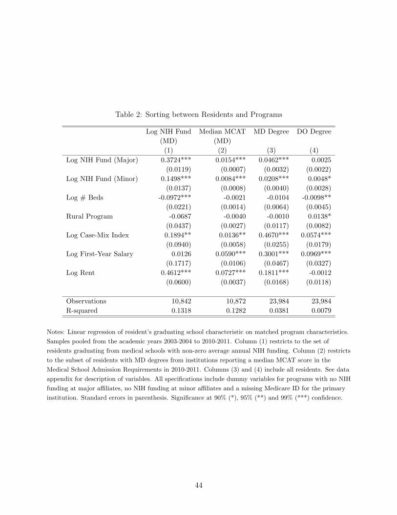
Table 2: Sorting between Residents and Programs

Log NIH Fund Median MCAT MD Degree DO Degree

(MD) (MD)

(1) (2) (3) (4)

Log NIH Fund (Major) 0.3724*** 0.0154*** 0.0462*** 0.0025

(0.0119) (0.0007) (0.0032) (0.0022)

Log NIH Fund (Minor) 0.1498*** 0.0084*** 0.0208*** 0.0048*

(0.0137) (0.0008) (0.0040) (0.0028)

Log # Beds -0.0972*** -0.0021 -0.0104 -0.0098**

(0.0221) (0.0014) (0.0064) (0.0045)

Rural Program -0.0687 -0.0040 -0.0010 0.0138*

(0.0437) (0.0027) (0.0117) (0.0082)

Log Case-Mix Index 0.1894** 0.0136** 0.4670*** 0.0574***

(0.0940) (0.0058) (0.0255) (0.0179)

Log First-Year Salary 0.0126 0.0590*** 0.3001*** 0.0969***

(0.1717) (0.0106) (0.0467) (0.0327)

Log Rent 0.4612*** 0.0727*** 0.1811*** -0.0012

(0.0600) (0.0037) (0.0168) (0.0118)

Observations 10,842 10,872 23,984 23,984

R-squared 0.1318 0.1282 0.0381 0.0079

Notes: Linear regression of resident’s graduating school characteristic on matched program characteristics.

Samples pooled from the academic years 2003-2004 to 2010-2011. Column (1) restricts to the set of

residents graduating from medical schools with non-zero average annual NIH funding. Column (2) restricts

to the subset of residents with MD degrees from institutions reporting a median MCAT score in the

Medical School Admission Requirements in 2010-2011. Columns (3) and (4) include all residents. See data

appendix for description of variables. All specifications include dummy variables for programs with no NIH

funding at major affiliates, no NIH funding at minor affiliates and a missing Medicare ID for the primary

institution. Standard errors in parenthesis. Significance at 90% (*), 95% (**) and 99% (***) confidence.

44

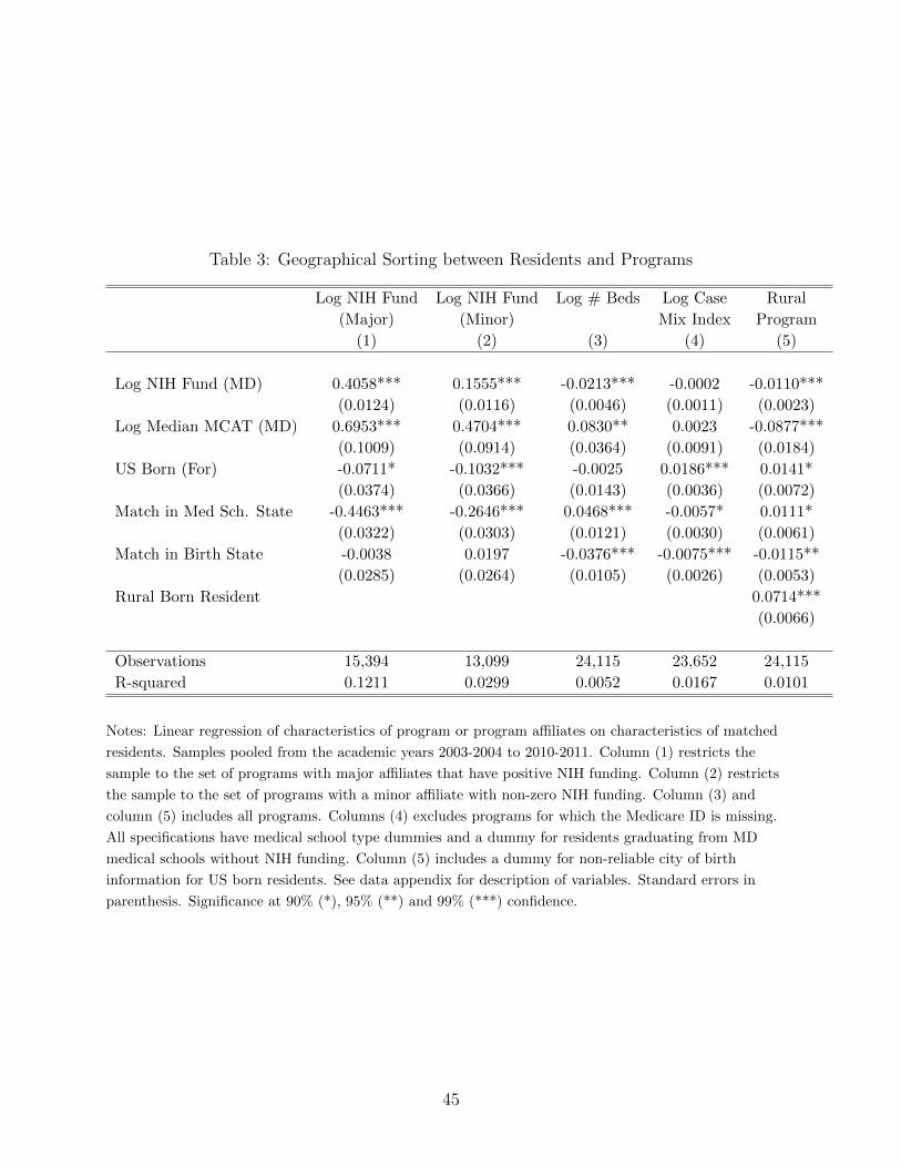
Table 3: Geographical Sorting between Residents and Programs

Log NIH Fund Log NIH Fund Log # Beds Log Case Rural

(Major) (Minor) Mix Index Program

(1) (2) (3) (4) (5)

Log NIH Fund (MD) 0.4058*** 0.1555*** -0.0213*** -0.0002 -0.0110***

(0.0124) (0.0116) (0.0046) (0.0011) (0.0023)

Log Median MCAT (MD) 0.6953*** 0.4704*** 0.0830** 0.0023 -0.0877***

(0.1009) (0.0914) (0.0364) (0.0091) (0.0184)

US Born (For) -0.0711* -0.1032*** -0.0025 0.0186*** 0.0141*

(0.0374) (0.0366) (0.0143) (0.0036) (0.0072)

Match in Med Sch. State -0.4463*** -0.2646*** 0.0468*** -0.0057* 0.0111*

(0.0322) (0.0303) (0.0121) (0.0030) (0.0061)

Match in Birth State -0.0038 0.0197 -0.0376*** -0.0075*** -0.0115**

(0.0285) (0.0264) (0.0105) (0.0026) (0.0053)

Rural Born Resident 0.0714***

(0.0066)

Observations 15,394 13,099 24,115 23,652 24,115

R-squared 0.1211 0.0299 0.0052 0.0167 0.0101

Notes: Linear regression of characteristics of program or program affiliates on characteristics of matched

residents. Samples pooled from the academic years 2003-2004 to 2010-2011. Column (1) restricts the

sample to the set of programs with major affiliates that have positive NIH funding. Column (2) restricts

the sample to the set of programs with a minor affiliate with non-zero NIH funding. Column (3) and

column (5) includes all programs. Columns (4) excludes programs for which the Medicare ID is missing.

All specifications have medical school type dummies and a dummy for residents graduating from MD

medical schools without NIH funding. Column (5) includes a dummy for non-reliable city of birth

information for US born residents. See data appendix for description of variables. Standard errors in

parenthesis. Significance at 90% (*), 95% (**) and 99% (***) confidence.

45

Table 4: Within Program Variation in Resident Characteristics

Fraction of Variation Within Program-Year

Log NIH Fund (MD) 77.83%

Median MCAT (MD) 72.09%

US Born Foreign Graudate 79.01%

Osteopathic/DO Degree 85.16%

Foreign Degree 57.16%

Allopathic/MD Degree 64.81%

Female 96.40%

Notes: Each row reports 1−R2adj from a separate linear regression of resident’s graduating school

characteristic absorbing the program-year fixed effects. Samples from the academic years 2003-2004 to

2010-2011. Samples for regressions with LHS variables Log NIH funding (MD), Median MCAT (MD) are

restricted to the set of residents with non-missing values for the respective characteristic. Regression of US

Born (For) restrict to graduates of foreign medical schools. Osteopathic/DO Degree, Foreign Degree,

Allopathic/MD Degree are linear probability models estimated on the full sample.

46

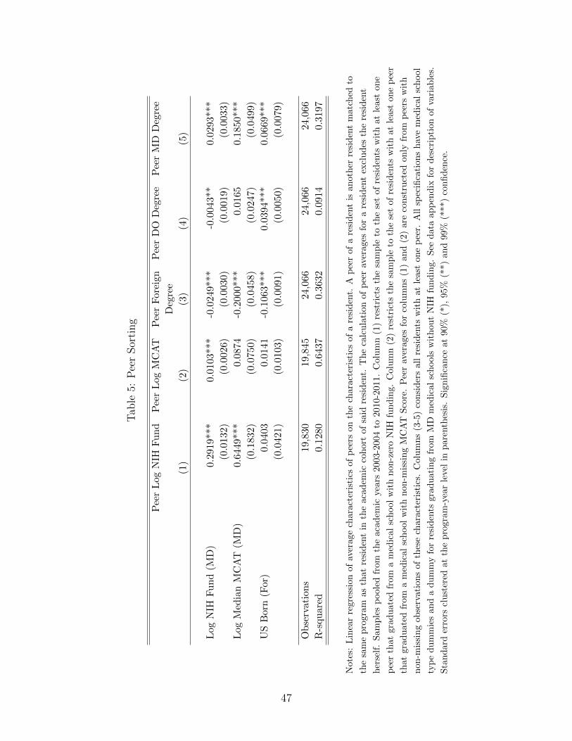
Tab

le5:

Pee

rSor

ting

Pee

rL

og

NIH

Fu

nd

Pee

rL

ogM

CA

TP

eer

For

eign

Pee

rD

OD

egre

eP

eer

MD

Deg

ree

Deg

ree

(1)

(2)

(3)

(4)

(5)

Log

NIH

Fu

nd

(MD

)0.

2919

***

0.01

03**

*-0

.024

9***

-0.0

043*

*0.

0293

***

(0.0

132)

(0.0

026)

(0.0

030)

(0.0

019)

(0.0

033)

Log

Med

ian

MC

AT

(MD

)0.

6449

***

0.08

74-0

.200

0***

0.01

650.

1850

***

(0.1

832)

(0.0

750)

(0.0

458)

(0.0

247)

(0.0

499)

US

Bor

n(F

or)

0.04

030.

0141

-0.1

063*

**0.

0394

***

0.06

69**

*

(0.0

421)

(0.0

103)

(0.0

091)

(0.0

050)

(0.0

079)

Ob

serv

ati

on

s19

,830

19,8

4524

,066

24,0

6624

,066

R-s

qu

are

d0.

1280

0.64

370.

3632

0.09

140.

3197

Not

es:

Lin

ear

regr

essi

onof

aver

age

char

acte

rist

ics

of

pee

rson

the

chara

cter

isti

csof

are

sid

ent.

Ap

eer

of

are

sid

ent

isan

oth

erre

sid

ent

matc

hed

to

the

sam

ep

rogr

amas

that

resi

den

tin

the

acad

emic

coh

ort

of

said

resi

den

t.T

he

calc

ula

tion

of

pee

rav

erages

for

are

sid

ent

excl

ud

esth

ere

sid

ent

her

self

.S

amp

les

pool

edfr

omth

eac

adem

icye

ars

2003-2

004

to2010-2

011.

Colu

mn

(1)

rest

rict

sth

esa

mp

leto

the

set

of

resi

den

tsw

ith

at

least

on

e

pee

rth

atgr

adu

ated

from

am

edic

alsc

hool

wit

hn

on

-zer

oN

IHfu

nd

ing.

Colu

mn

(2)

rest

rict

sth

esa

mp

leto

the

set

of

resi

den

tsw

ith

at

least

on

ep

eer

that

grad

uat

edfr

oma

med

ical

sch

ool

wit

hn

on-m

issi

ng

MC

AT

Sco

re.

Pee

rav

erages

for

colu

mn

s(1

)an

d(2

)are

con

stru

cted

on

lyfr

om

pee

rsw

ith

non

-mis

sin

gob

serv

atio

ns

ofth

ese

char

acte

rist

ics.

Colu

mn

s(3

-5)

con

sid

ers

all

resi

den

tsw

ith

at

least

on

ep

eer.

All

spec

ifica

tion

sh

ave

med

ical

sch

ool

typ

ed

um

mie

san

da

du

mm

yfo

rre

sid

ents

grad

uati

ng

from

MD

med

ical

sch

ools

wit

hou

tN

IHfu

nd

ing.

See

data

ap

pen

dix

for

des

crip

tion

of

vari

ab

les.

Sta

nd

ard

erro

rscl

ust

ered

atth

epro

gram

-yea

rle

vel

inp

are

nth

esis

.S

ign

ifica

nce

at

90%

(*),

95%

(**)

an

d99%

(***)

con

fid

ence

.

47

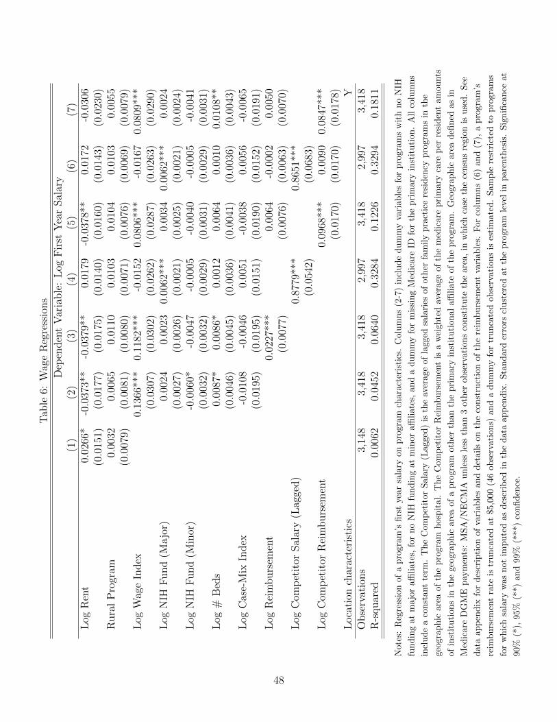
Tab

le6:

Wag

eR

egre

ssio

ns

Dep

enden

tV

aria

ble

:L

ogF

irst

Yea

rSal

ary

(1)

(2)

(3)

(4)

(5)

(6)

(7)

Log

Ren

t0.

0266

*-0

.037

3**

-0.0

379*

*0.

0179

-0.0

378*

*0.

0172

-0.0

306

(0.0

151)

(0.0

177)

(0.0

175)

(0.0

140)

(0.0

160)

(0.0

143)

(0.0

230)

Rura

lP

rogr

am0.

0032

0.00

650.

0110

0.01

030.

0104

0.01

030.

0055

(0.0

079)

(0.0

081)

(0.0

080)

(0.0

071)

(0.0

076)

(0.0

069)

(0.0

079)

Log

Wag

eIn

dex

0.13

66**

*0.

1182

***

-0.0

152

0.08

06**

*-0

.016

70.

0809

***

(0.0

307)

(0.0

302)

(0.0

262)

(0.0

287)

(0.0

263)

(0.0

290)

Log

NIH

Fund

(Majo

r)0.

0024

0.00

230.

0062

***

0.00

340.

0062

***

0.00

24(0

.002

7)(0

.002

6)(0

.002

1)(0

.002

5)(0

.002

1)(0

.002

4)L

ogN

IHF

und

(Min

or)

-0.0

060*

-0.0

047

-0.0

005

-0.0

040

-0.0

005

-0.0

041

(0.0

032)

(0.0

032)

(0.0

029)

(0.0

031)

(0.0

029)

(0.0

031)

Log

#B

eds

0.00

87*

0.00

86*

0.00

120.

0064

0.00

100.

0108

**(0

.004

6)(0

.004

5)(0

.003

6)(0

.004

1)(0

.003

6)(0

.004

3)L

ogC

ase-

Mix

Index

-0.0

108

-0.0

046

0.00

51-0

.003

80.

0056

-0.0

065

(0.0

195)

(0.0

195)

(0.0

151)

(0.0

190)

(0.0

152)

(0.0

191)

Log

Rei

mburs

emen

t0.

0227

***

0.00

64-0

.000

20.

0050

(0.0

077)

(0.0

076)

(0.0

063)

(0.0

070)

Log

Com

pet

itor

Sal

ary

(Lag

ged)

0.87

79**

*0.

8651

***

(0.0

542)

(0.0

683)

Log

Com

pet

itor

Rei

mburs

emen

t0.

0968

***

0.00

900.

0847

***

(0.0

170)

(0.0

170)

(0.0

178)

Loca

tion

char

acte

rist

ics

YO

bse

rvat

ions

3,14

83,

418

3,41

82,

997

3,41

82,

997

3,41

8R

-squar

ed0.

0062

0.04

520.

0640

0.32

840.

1226

0.32

940.

1811

Not

es:

Reg

ress

ion

ofa

pro

gram

’sfi

rst

year

sala

ryon

pro

gra

mch

ara

cter

isti

cs.

Colu

mn

s(2

-7)

incl

ud

ed

um

my

vari

ab

les

for

pro

gra

ms

wit

hno

NIH

fun

din

gat

ma

jor

affili

ates

,fo

rn

oN

IHfu

nd

ing

at

min

or

affi

liate

s,an

da

du

mm

yfo

rm

issi

ng

Med

icare

IDfo

rth

ep

rim

ary

inst

itu

tion

.A

llco

lum

ns

incl

ud

ea

con

stan

tte

rm.

Th

eC

omp

etit

orS

alar

y(L

agged

)is

the

aver

age

of

lagged

sala

ries

of

oth

erfa

mil

yp

ract

ice

resi

den

cyp

rogra

ms

inth

e

geog

rap

hic

area

ofth

ep

rogr

amh

osp

ital

.T

he

Com

pet

itor

Rei

mb

urs

emen

tis

aw

eighte

dav

erage

of

the

med

icare

pri

mary

care

per

resi

den

tam

ou

nts

ofin

stit

uti

ons

inth

ege

ogra

ph

icar

eaof

ap

rogr

am

oth

erth

an

the

pri

mary

inst

itu

tion

al

affi

liate

of

the

pro

gra

m.

Geo

gra

ph

icare

ad

efin

edas

in

Med

icar

eD

GM

Ep

aym

ents

:M

SA

/NE

CM

Au

nle

ssle

ssth

an

3oth

erob

serv

ati

on

sco

nst

itu

teth

eare

a,

inw

hic

hca

seth

ece

nsu

sre

gio

nis

use

d.

See

dat

aap

pen

dix

for

des

crip

tion

ofva

riab

les

and

det

ail

son

the

con

stru

ctio

nof

the

reim

bu

rsem

ent

vari

ab

les.

For

colu

mn

s(6

)an

d(7

),a

pro

gra

m’s

reim

bu

rsem

ent

rate

istr

un

cate

dat

$5,0

00(4

6ob

serv

ati

on

s)and

ad

um

my

for

tru

nca

ted

ob

serv

ati

on

sis

esti

mate

d.

Sam

ple

rest

rict

edto

pro

gra

ms

for

wh

ich

sala

ryw

asn

otim

pu

ted

asd

escr

ibed

inth

ed

ata

ap

pen

dix

.S

tan

dard

erro

rscl

ust

ered

at

the

pro

gra

mle

vel

inp

are

nth

esis

.S

ign

ifica

nce

at

90%

(*),

95%

(**)

and

99%

(***

)co

nfi

den

ce.

48

Table 7: Preference Estimates

Full Geographic Geo. Het. w/

Heterogeneity Heterogeneity Wage Instrument

(1) (2) (3)

Panel A.1: Preference for Programs (in $ for one std. dev. change)Case Mix Index

Coeff 4,792 2,320 6,088

(1,624) (1,265) (1,542)

Sigma RC 4,503

(1,037)

Log NIH Fund (Major)

Coeff 491 6,499 4,402

(1,651) (2,041) (1,333)

Sigma RC 5,498

(1,234)

Log Beds

Coeff 6,900 3,528 8,837

(2,207) (1,259) (1,936)

Sigma RC 11,107

(2,073)

Log NIH Fund (Minor) 4,993 5,560 7,620

(1,558) (1,511) (1,821)

Panel A.2: Preference for Programs (in $)Rural Program 7,327 5,611 17,314

(3,492) (3,555) (4,938)

University Based Program 15,786 11,080 25,130

(3,982) (5,393) (7,088)

Community/University Program -5,001 -2,217 -7,507

(2,016) (1,589) (2,233)

Medical School State 9,820 2,302 4,529

(1,998) (687) (910)

Birth State 6,342 1,320 2,451

(1,308) (411) (497)

Rural Birth x Rural Program 1,189 109 233

(466) (113) (102)

(cont’d...)

49

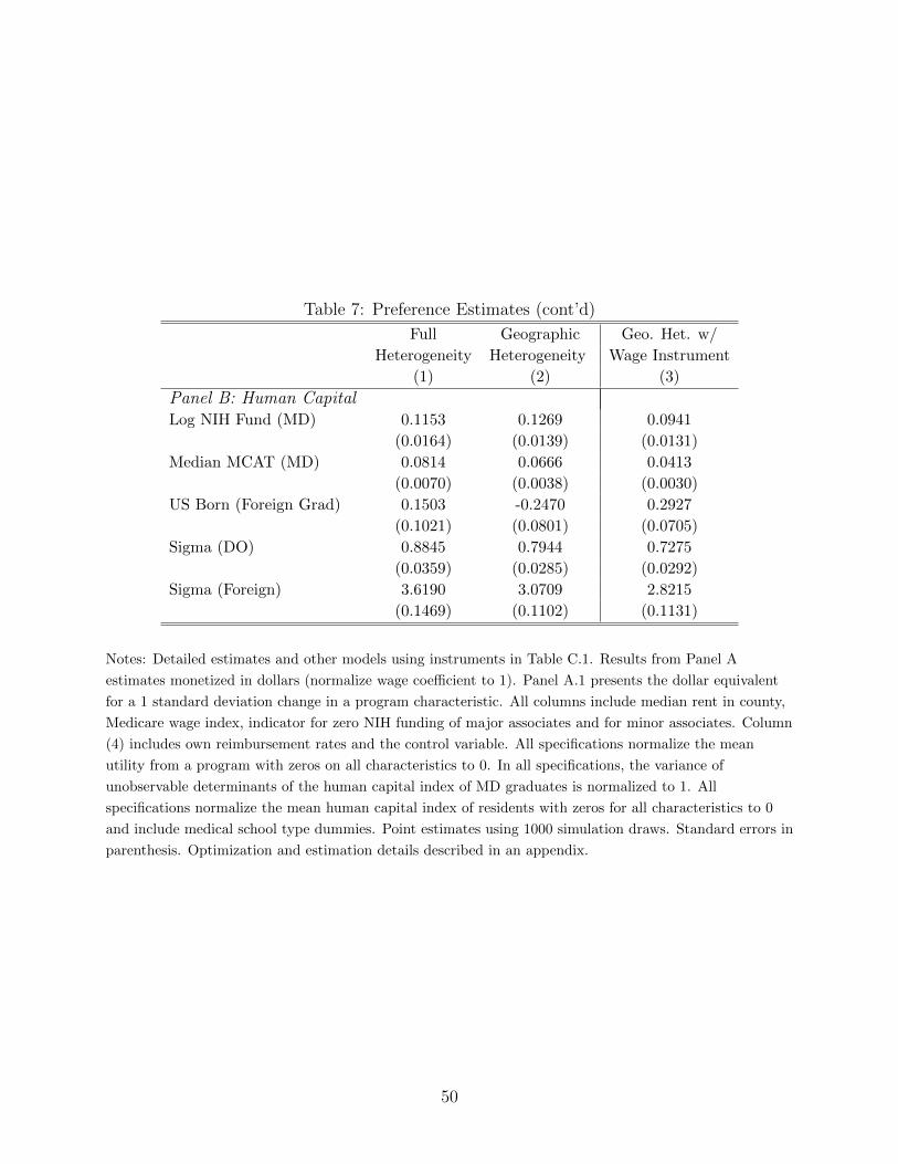
Table 7: Preference Estimates (cont’d)

Full Geographic Geo. Het. w/

Heterogeneity Heterogeneity Wage Instrument

(1) (2) (3)

Panel B: Human CapitalLog NIH Fund (MD) 0.1153 0.1269 0.0941

(0.0164) (0.0139) (0.0131)

Median MCAT (MD) 0.0814 0.0666 0.0413

(0.0070) (0.0038) (0.0030)

US Born (Foreign Grad) 0.1503 -0.2470 0.2927

(0.1021) (0.0801) (0.0705)

Sigma (DO) 0.8845 0.7944 0.7275

(0.0359) (0.0285) (0.0292)

Sigma (Foreign) 3.6190 3.0709 2.8215

(0.1469) (0.1102) (0.1131)

Notes: Detailed estimates and other models using instruments in Table C.1. Results from Panel A

estimates monetized in dollars (normalize wage coefficient to 1). Panel A.1 presents the dollar equivalent

for a 1 standard deviation change in a program characteristic. All columns include median rent in county,

Medicare wage index, indicator for zero NIH funding of major associates and for minor associates. Column

(4) includes own reimbursement rates and the control variable. All specifications normalize the mean

utility from a program with zeros on all characteristics to 0. In all specifications, the variance of

unobservable determinants of the human capital index of MD graduates is normalized to 1. All

specifications normalize the mean human capital index of residents with zeros for all characteristics to 0

and include medical school type dummies. Point estimates using 1000 simulation draws. Standard errors in

parenthesis. Optimization and estimation details described in an appendix.

50

Table 8: Estimated Utility Distribution in First-Year Salary Equivalent

Full Geographic Geo. Het. w/Heterogeneity Heterogeneity Wage Instrument

(1) (2) (3)N Stat (s.e.) Stat (s.e.) Stat (s.e.)

Panel A: Means in CategoryLog Beds (Primary Inst)

Lowest Quartile 107 -$12,509 (3,290) -$5,691 (777) -$15,238 (4,647)Second Quartile 107 -$2,801 (758) -$3,693 (553) -$3,606 (1,212)Third Quartile 107 $3,823 (1,138) -$1,041 (320) $1,934 (1,108)Highest Quartile 107 $11,487 (2,877) $10,425 (1,327) $16,910 (4,831)

Case Mix IndexLowest Quartile 107 -$10,397 (2,880) -$4,045 (674) -$10,556 (3,450)Second Quartile 107 -$3,764 (1,100) -$1,965 (436) -$5,162 (1,643)Third Quartile 107 $3,346 (1,179) -$1,518 (403) $669 (720)Highest Quartile 107 $10,815 (2,849) $7,528 (1,196) $15,050 (4,663)

Log NIH Fund (Major)Lowest Quartile 71 -$5,190 (1,716) -$7,903 (1,064) -$15,032 (4,267)Second Quartile 71 -$3,712 (1,080) -$285 (390) -$8,095 (2,685)Third Quartile 71 $1,796 (963) $8,460 (1,274) $6,646 (2,021)Highest Quartile 72 $904 (1,535) $11,733 (1,736) $7,194 (2,368)

County RentLowest Quartile 106 -$5,681 (1,580) -$6,745 (984) -$11,796 (3,549)Second Quartile 107 -$1,012 (541) -$964 (244) -$3,310 (1,077)Third Quartile 99 $1,984 (688) $1,715 (333) $2,942 (1,204)Highest Quartile 116 $4,431 (1,321) $5,589 (827) $11,321 (3,148)

Rural Program 63 -$7,292 (3,101) -$4,692 (967) -$8,066 (4,044)Urban Program 365 $1,259 (535) $810 (167) $1,392 (698)

Overall Std. Dev. 428 $21,937 (5,215) $14,088 (1,880) $28,578 (8,166)

Notes: Utilities net of salaries are monetized in dollars and normalized to an overall mean of zero.

Statistics averages across residents from 100 simulation draws. Each simulation draws a parameter from a

normal with mean θMSM and variance Σ, where Σ is estimated as described in Section 6.4. Statistics use

the 2010-2011 sample.

51

Table 9: Implicit Tuition

Full Geographic Geo. Het. w/

Heterogeneity Heterogeneity Wage Instrument

(1) (2) (3)

Mean $23,802.64 $22,627.64 $43,470.39

(5526.15) (3495.62) (13678.08)

Median $21,263.30 $21,167.71 $40,606.85

(5076.79) (3265.54) (12847.51)

Standard Deviation $16,661.17 $12,278.42 $24,792.30

(3946.33) (1781.09) (7485.20)

5th Percentile $2,795.23 $5,179.08 $7,912.03

(1008.51) (1441.71) (3246.19)

25th Percentile $11,648.70 $14,070.10 $24,853.10

(2820.62) (2364.41) (8299.05)

75th Percentile $31,467.42 $28,902.46 $58,354.66

(7131.65) (4347.95) (18134.03)

95th Percentile $55,279.76 $45,784.76 $92,343.91

(12758.48) (6921.96) (28071.67)

Notes: Based on 100 simulation draws. Each simulation draws a parameter from a normal with mean

θMSM and variance Σ, where Σ is estimated as described in Section 6.4. Standard errors in parenthesis.

52

Table 10: Dependence of Implicit Tuition on Demand-Supply Imbalance

Log Average Implicit Tuition in Program

Full Heterogeneity

(1) (2) (3) (4)

Log Residency Positions 0.0008 -0.1557*** -0.0578*** -0.1442***

in Program State (0.0044) (0.0106) (0.0101) (0.0128)

Log Family Medicine MD Graduates 0.1851*** 0.1951***

from Program State (0.0114) (0.0130)

Log US Born Residents 0.0658*** -0.0233

in Program State (0.0102) (0.0145)

R-squared 0.4144 0.4180 0.4150 0.4180

Notes: Linear Regressions. Dependent variable is the log of total implicit tuition at a residency program

divided by the number of residents matched to the program. All regressions on generated implicit tuitions

data using the 2010-2011 sample of residents and programs, and 100 simulation draws. All regressions

include Log Beds, Log NIH Fund (Major), Log NIH Fund (Minor), dummies for no NIH funded affiliated,

Medicare Case Mix Index, Rural Program dummy and Program type dummies. Standard errors clustered

at the simulation level. Significance at 90% (*), 95% (**) and 99% (***) confidence.

53

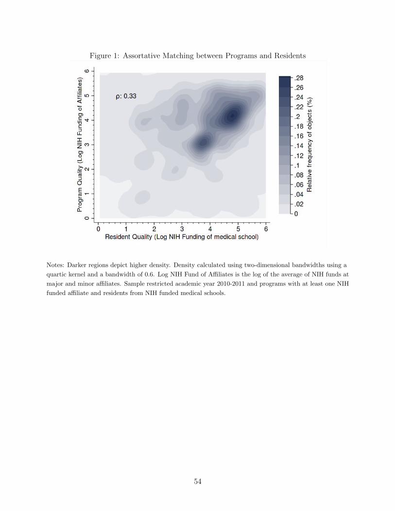
Figure 1: Assortative Matching between Programs and Residents

Notes: Darker regions depict higher density. Density calculated using two-dimensional bandwidths using a

quartic kernel and a bandwidth of 0.6. Log NIH Fund of Affiliates is the log of the average of NIH funds at

major and minor affiliates. Sample restricted academic year 2010-2011 and programs with at least one NIH

funded affiliate and residents from NIH funded medical schools.

54

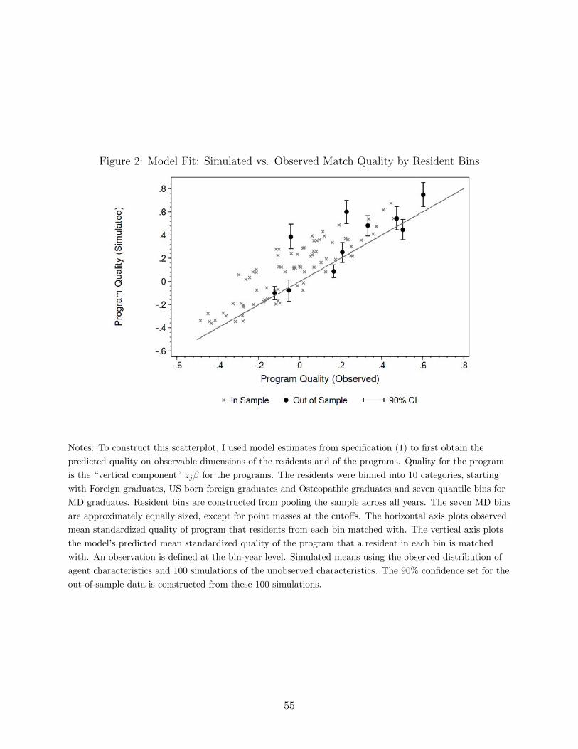
Figure 2: Model Fit: Simulated vs. Observed Match Quality by Resident Bins

Notes: To construct this scatterplot, I used model estimates from specification (1) to first obtain the

predicted quality on observable dimensions of the residents and of the programs. Quality for the program

is the “vertical component” zjβ for the programs. The residents were binned into 10 categories, starting

with Foreign graduates, US born foreign graduates and Osteopathic graduates and seven quantile bins for

MD graduates. Resident bins are constructed from pooling the sample across all years. The seven MD bins

are approximately equally sized, except for point masses at the cutoffs. The horizontal axis plots observed

mean standardized quality of program that residents from each bin matched with. The vertical axis plots

the model’s predicted mean standardized quality of the program that a resident in each bin is matched

with. An observation is defined at the bin-year level. Simulated means using the observed distribution of

agent characteristics and 100 simulations of the unobserved characteristics. The 90% confidence set for the

out-of-sample data is constructed from these 100 simulations.

55

Appendix

Appendices C, D, E and F are available online.

A Estimation Appendix

A.1 A Bootstrap

The bootstrap mimics the following data generating process. The number of programs ina given market is denoted Jt. Each program has a capacity cjt that is drawn iid froma distribution Fc with support on the natural numbers less than c. The total number ofpositions in market t is the random variable Ct =

∑cjt. In each market, the number of

residents Nt is drawn from a binomial distribution B (Ct, pt) for pt ≤ 1. The vector of residentand program characteristics (zjt, zijt, xi, rjt, εi, βi, ηjt, ζjt) are independently sampled from apopulation distribution. The distribution of program observable characteristics (zjt, zijt)may depend on cjt while all other characteristics are drawn independently.

The estimation error in θmsm is approximated as

Σ =(

Γ′W Γ)−1

Γ′W

(V +

1

SV S

)W ′Γ

(Γ′W Γ

)−1,

where W is the weight matrix used in the objective function, Γ = Γ (θ0) is the gradient ofm (θ) evaluated at θ0, and V tot is the asymptotic variance in mS (θ0), and J =

∑Jt. The

asymptotic variance V tot in m (θ0) is the sum of the variance due to two independent process:the sampling variance V arising from sampling the observable characteristics of residents andprograms in the economy and the simulation variance VS due to the sampling unobservabletraits of the residents and programs. I use numerical and simulation techniques to estimateeach of the unknown quantities Γ, VS, V tot.

To estimate Γ (θ0), I construct two-sided numerical derivatives of the simulated momentfunction m (θ) using the observed population of residents and programs. Since mS (θ) isnot smooth due to simulation errors, I use 10,000 simulation draws and a step size of 10−3.The simulation variance is estimated by calculating the variance in 10,000 evaluations of

mS(θmsm

), each with a single simulation draw and using the observed sample of resident

and program characteristics. These two quantities can be calculated independently in eachof the markets.

In models using a wage instrument, the sampling variance in m (θ) needs to account forthe fact that the control variable νjt is estimated. It also needs to account for the dependentstructure of the match data. I use the following bootstrap procedure to estimate V .

1. For each market t, sample Jt program observable characteristics from the observed

data {zjt, rjt, qjt}Jtj=1 with replacement. Denote this sample with{zbjt, r

bjt, q

bjt

}Jtj=1

(a) Calculate(γb, τ b

)and the estimated control variables νbjt as in the estimation step.

This step is skipped in models treating salaries as exogenous.

56

2. Draw N bt from B

(∑Jtj=1 q

bjt,

Nt

Qt

)and a sample of resident and resident-program specific

observables{xbit,{zbijt}Jtj=1

}Nbt

i=1from the observed data, with replacement.

3. Simulate the unobservables to compute{m1,b

(θmsm

)}Bb=1

the vector of simulated mo-

ments using the bootstrap sample economy. The variance of these moments is theestimate I use for V .

The bootstrap replaces the population distribution of observed characteristics of theresidents and programs with the empirical distribution observed in the data. Given a sampledeconomy, it computes νjt and the moments at a pairwise stable match at θ. The covariance

of the moments across bootstrap iterations is the estimate of V . The uncertainty due tosimulation error V S is approximated by drawing just the unobserved characteristics fromthe assumed parametric distribution.

The method yields consistent estimates for standard errors if the equilibrium map from θand the distribution market participants to the data is smooth. Standard Donsker theoremsapply for the sampling process for market participants. The inference method above shouldthen be consistent if a functional delta method applies to this map i.e. the distribution ofthe moments is (Hadamard) differentiable jointly in the parameter θ and the distribution ofobserved characteristics of market participants.

A.2 Weight Matrix

It is well known that the choice of weight matrix can affect efficiency, particularly when thenumber of moments is much larger than the number of parameters. A common method usesa first stage consistent estimate of θ0 to obtain variance estimates V and V S to compute the

optimal weight matrix W =(V + 1

SV S)−1

that can be used in the second stage. In this

application, a two-step procedure is computationally prohibitive. In Monte Carlo simulationswith this dataset and I found that using the identity matrix was often inaccurate and leftus with a poor estimate of θ0. Intuitively, the identity matrix fails to account for theco-variance in the various program and resident characteristics as well as the covariancewith the within-program moments. To appropriately weight some of these aspects, I usea weight matrix W that is calculated using the following bootstrap procedure seemed toapproximate the optimal weights fairly well. For each market t, with replacement, randomlysample Jt programs and the residents matched with them. Treat the observed matches

as the matches in the bootstrap sample as well.44 Compute moments{mb}Bb=1

from the

sample and compute the variance V and set W = V −1. While this weight matrix need notconverge to the optimal weight matrix, the only theoretical loss is in the efficiency of theestimator. This weight matrix also turns out to be close to one that would be calculated as

W =(V(θmsm

)+ 1

SV S(θmsm

))−1where θmsm is the estimate of θ0 using W as the weight

matrix.

44Note that a submatch of a stable match is also stable. Hence, the constructed bootstrap match is alsostable.

57

B Wage Competition

B.1 Expressions for Competitive Outcomes

I first characterize the competitive equilibria of the model. The expression in equation (13)follows as a corollary. For clarity, I refer to the quality of program 1 as q1 although I normalizeit to 0 in the model presented in the text.

Proposition 3 The wage wk paid to resident k by program k in a competitive equilibriumis characterized by

w1 ∈ [−aq1, f (h1, q1)]

wk − wk−1 + a (qk − qk−1) ∈ [f (hk, qk−1)− f (hk−1, qk−1) , f (hk, qk)− f (hk−1, qk)]

Proof. Since the competitive equilibrium maximizes total surplus, resident i is matchedwith program i in a competitive equilibrium. The wages are characterized by

IC (k, i) : f (hk, qk)− wk ≥ f (hi, qk)− wi + a (qk − qi)IR (k) : aqk + wk ≥ 0, wk ≤ f (hk, qk) .

First, I show that IR (k) is slack for k > 1 as long as IR (1) and IC (k, i) are satisfiedfor all i, k. Since IC (1, k) is satisfied,

f (h1, q1)− w1 ≥ f (hk, q1)− wk + a (q1 − qk)⇒ wk ≥ w1 + f (hk, q1)− f (h1, q1) + a (q1 − qk)

≥ −aqk (16)

where the last inequality follows from f (hk, q1) − f (h1, q1) ≥ 0 and w1 + aq1 ≥ 0 from theIR (1) . Also, IC (k, 1) implies that

f (hk, qk)− wk ≥ f (h1, qk)− w1 + a (qk − q1)⇒ wk ≤ f (hk, qk)− f (h1, qk) + w1 − a (qk − q1)

≤ f (hk, qk)− f (h1, q1) + w1 − a (qk − q1)≤ f (hk, qk) (17)

where the last two inequalities follow since w1 ≤ f (h1, q1) from IR (1) and −a (qk − q1) ≤ 0.Equations (16) and (17) imply IR (k).

Second, I show that it is sufficient to only consider local incentive constraints, i.e.IC (i, i− 1) and IC (i, i+ 1) for all i imply IC (k,m) for all k, m. Assume that IC (i, i− 1)is satisfied for all i. For firms i ∈ {m, . . . , k}, this hypothesis implies that

f (hi, qi)− wi ≥ f (hi−1, qi)− wi−1 + a (qi − qi−1) .

58

Summing each side of the inequality from i = m to k yields that

f (hk, qk)− wk ≥k∑

i=m+1

[f (hi−1, qi)− f (hi−1, qi−1)] + f (hm−1, qm) + a (qk − qm−1)− wm−1.

Since each f (hi−1, qi)− f (hi−1, qi−1) ≥ f (hm−1, qi)− f (hm−1, qi−1) for i ≥ m,

f (hk, qk)− wk

≥k∑

i=m+1

[f (hm−1, ql)− f (hm−1, qi−1)] + f (hm−1, qm) + a (qk − qm−1)− wm−1

= f (hm−1, qk) + a (qk − qm−1)− wm−1. (18)

Hence, IC (k,m) is satisfied for all m ∈ {1, . . . , k}. A symmetric argument shows that ifIC (i, i+ 1) is satisfied for all k, then IC (k,m) is satisfied for all m ∈ {k, . . . , N}

To complete the proof, note that local ICs yield the desired upper and lower bounds.

Corollary 4 The worker optimal competitive equilibrium wages are given by

wk = f (h1, q1)− a (qk − q1) +k∑i=2

[f (hi, qi)− f (hi−1, qi)]

and the firm optimal competitive equilibrium wages are given by

wk = −a (qk − q1) +k∑i=2

[f (hi, qi−1)− f (hi−1, qi−1)]

B.2 Proof of Proposition 1

Consider an N -vector of outputs y = (y1, . . . , yk) and define a family of production functionsF (y) = {f : f (hk, qk) = yk} where yk denotes the output produced by the pair (hk, qk) . Thetwo extremal technologies in this family are given by fy (hk, ql) = yk and fy (hl, qk) = yk for

all l ∈ {1, . . . , N}. Let wfok (f) (likewise wwo (f)) denote the firm-optimal (worker-optimal)competitive wage under technology f .

I prove a slightly stronger result here as it may be of independent interest. This resultshows that the split of surplus in cases other than f and f are intermediate.

Theorem 5 In the worker-optimal (firm-optimal) competitive equilibria, each worker’s wagefor all f ∈ F (y) is bounded above by her wage under fy and below by her wage under fy.

Hence, for all f ∈ F (y), the set of competitive equilibrium wages of worker k is bounded

below by wfok

(fy

)= −aqk and above by wwok

(fy)

= yk − aqk.

Proof. I only derive the bounds for the worker optimal equilibrium since the calculation for

59

the firm optimal equilibrium is analogous. From the expressions in corollary 4,

wwok

(fy

)= fy (h1, q1)− a (qk − q1)

= y1 − a (qk − q1)

since the terms in the summation are identically 0. For any production function, f ∈ F (y),

wwok (f) = f (h1, q1)− a (qk − q1) +k∑i=2

[f (hi, qi)− f (hi−1, qi)]

≥ y1 − a (qk − q1) = wwok

(fy

)since f (h1, q1) = y1 and f (hi, qi)− f (hi−1, qi) ≥ 0. Similarly, note that

wwok(fy)

= yk − a (qk − q1)

and since each f (hi, qi)− f (hi−1, qi) ≤ f (hi, qi)− f (hi−1, qi−1),

wwok (f) ≤ f (hk, qk)− a (qk − q1)= yk − a (qk − q1) = wwok

(fy).

Proposition 1 follows as a corollary:Proof. For any y = (y1, . . . , yk) and production function f ∈ F (y), the profit of firm k isgiven by

f (hk, qk)− wk = yk − wk≥ yk − wwok

(fy)

= a (qk − q1)

B.3 Implicit Tuition

I prove a more general result for many-to-one assignment games that subsumes Proposition2. A many to one assignment game between workers i ∈ {1, . . . , N} and firms j ∈ {1, . . . , J}is defnited by the capacity of firsm firms cj and the surplus aij produced by the worker-firmpair (i, j). The surplus from multiple workers is additively separable and an empty positionproduces 0. I focus on the case when

∑j cj ≥ N . I micro-found the surplus as the sum,

afij = uij + f (hi), of the production f (hi) ≥ 0 produced by a worker with human capital hiand the utility worker i receives from working at firm j at a wage of w, given uij+w. I assumethat each uij ≥ 0. For completeness, I define a few concepts below. Rigorous treatments ofthese concepts for the one-to-one case are given in Roth and Sotomayor (1992), in Camina(2006) and Sotomayor (1999) for the many-to-one case.

An assignment is a vector x = {xij}i,j where xij = {0, 1} and xij = 1 denotes that i is

60

assigned to j. The assignment x is feasible if∑

i xij ≤ 1 and∑

j xij ≤ cj. In the many-

to-one case, we refer to an assignment of positions {yi,p}i,p where p ∈{

1, . . . ,∑

j cj

}denotes a position p and a firm. Let jp denote the firm offering position p. Each assignmentx induces a unique canonical assignment of positions y where the positions in the firm arefilled by residents in order of their index i.

An allocation is the pair (y, w) of an assignment of positions y and wages w = {wij}ijwith wij ∈ R. The surplus of position p is defined as vfp =

∑yip (f (hi)− wip) and of worker

i by ufi =∑yip(uijp + wip

). An outcome is a pair ((u, v) ; y) of payoffs u = {ui}i and

v = {vp}p and an assignment of positions y.A feasible outcome ((u, v) ; y) is stable if for all i, p, ui ≥ 0, vp ≥ 0, ui + vp ≥ aijp if

yip = 1 or xijp = 0, where x is the assignment corresponding to y. Consequently, unmatchedworker and firms can block if they can produce agree to a mutually beneficial outcome.A matched worker and firm pair can also block an outcome if the sum of their payoffs islower than the total surplus they produce. The correspondence between many to one stableoutcomes and competitive equilibria is noted in Camina (2006).

Now, we are ready to prove the desired result from which the one-to-one matching casefollows trivially by allowing for only one position at each firm.

Proposition 6 The equilibrium assignment of positions for the games afij and afij coincide.

Further, if ufi and vfp are position payoffs for the game af , then ufi = ufi +(f (hi)− f (hi)

)and vfp = vfp are equilibrium payoffs under the surplus afij. Consequently the implicit tuition

for each position is the same for the games af and af .

Proof. Sotomayor (1999) shows that equilibria for af and af exist and maximize the total

surplus in the set of feasible assignments. Towards a contradiction, assume that yf is an

equilibrium for af but not for af . The feasibility constraints are identical in the two games,

and so both yf and yf are feasible for both games. Since yf maximizes the total surplus

under af , ∑i,p

afijpyfip >

∑i,p

afijyfip

⇒∑i,p

afijpyfip +

∑i

∑p

(f (hi)− f (hi)

)yfip >

∑i,p

afijpyfip +

∑i

∑p

(f (hi)− f (hi)

)yfip. (19)

Since every worker-firm pair produces positive surplus and the total capacity exceeds thenumber of workers, there cannot be any unassigned workers in any feasible surplus maximiz-

ing allocation, i.e.∑

p yfip =

∑p y

fip = 1 for all i. Hence, we have that

∑p

(f (hi)− f (hi)

)yfip

=∑

i

(f (hi)− f (hi)

)yfij. The inequality in equation (19) reduces to

∑i,p a

fijpyfip >

∑i,p a

fijpyfip,

a contradiction to the assumption that yf is an equilibrium assignment for yf . This contra-diction implies that the equilibrium assignments of positions under the two games coincide.

To show that the second part of the result, consider the payoffs for af∗

where f ∗ (hi) =

max{f (hi) , f (hi)

}. I show that uf

∗

i = ufi +(f ∗ (hi)− f (hi)) and vf∗p = vfp . The comparison

61

of equilibrium payoffs for f and f follows immediately from this. Note that for all i and p,ufi ≥ 0 and vfj ≥ 0 implies vf

∗

j ≥ 0 and uf∗

i ≥ 0 since f ∗ (hi)− f (hi) ≥ 0. It remains to that

uf∗

i + vf∗p ≥ af

∗

ijpif i is assigned to position p or if i is not assigned to firm jp. Note that for

all i and p, we have that if ufi + vfp ≥ afip,

uf∗

i + vf∗

p = ufi + f ∗ (hi)− f (hi) + vfp

≥ afijp + f ∗ (hi)− f (hi)

= af∗

ijp.

To complete the proof I need to show that the payoffs to each position coincides underthe worker-optimal stable outcome. Let ufi and vfp denote this outcome for the game af .Let u0i and v0p be the worker-optimal outcome under the function f (hi) = 0 for all hi. Ishowed earlier that the optimal assignments coincide for these two cases. I have shown thatu0i + f (hi) and v0p is stable for af . Towards a contradiction, assume that ufi ≥ u0i + f (hi)

with strict inequality for at least one i. This implies that ufi − f (hi) is stable for a0. Hence,ufi − f (hi) ≥ u0i with strict inequality for at least one i, contradicting the assumption thatu0i and v0p are part of the worker-optimal outcome. If y is the optimal assignment, this shows

that v0p =∑

i yip(a0ip − u0i

)=∑

i yip

(afip − u

fi

)= vfp , proving the result.

B.4 Worker Optimal Equilibrium: Algorithm

The first step uses a linear program to solve for the assignment that produces the maximumtotal surplus. Let aij be the total surplus produced by the match of resident i with programj. This surplus is the sum of the value of the product produced by resident i at programj and the dollar value of resident i’s utility for program j at a wage of 0.45 With an abuseof notation of the letter x, let xij denote the (fraction) of resident i that is matched withprogram j. Sotomayor (1999) shows that the surplus maximizing (fractional) assignment isthe solution to the linear program

max{xij}

∑xijaij (20)

subject to

0 ≤ xij ≤ 1∑j

xij ≤ 1∑i

xij ≤ cj.

45As mentioned in footnote 41, I assume that the equilibrium is characterized by full employment. Ifutilities are normalized so that an allocation is individual rationality if the resident obtains non-negativeutility, then αij at the resident i’s least preferred program j must exceed the negative of the dollar monetizedutility resident i obtains at j at a wage of zero.

62

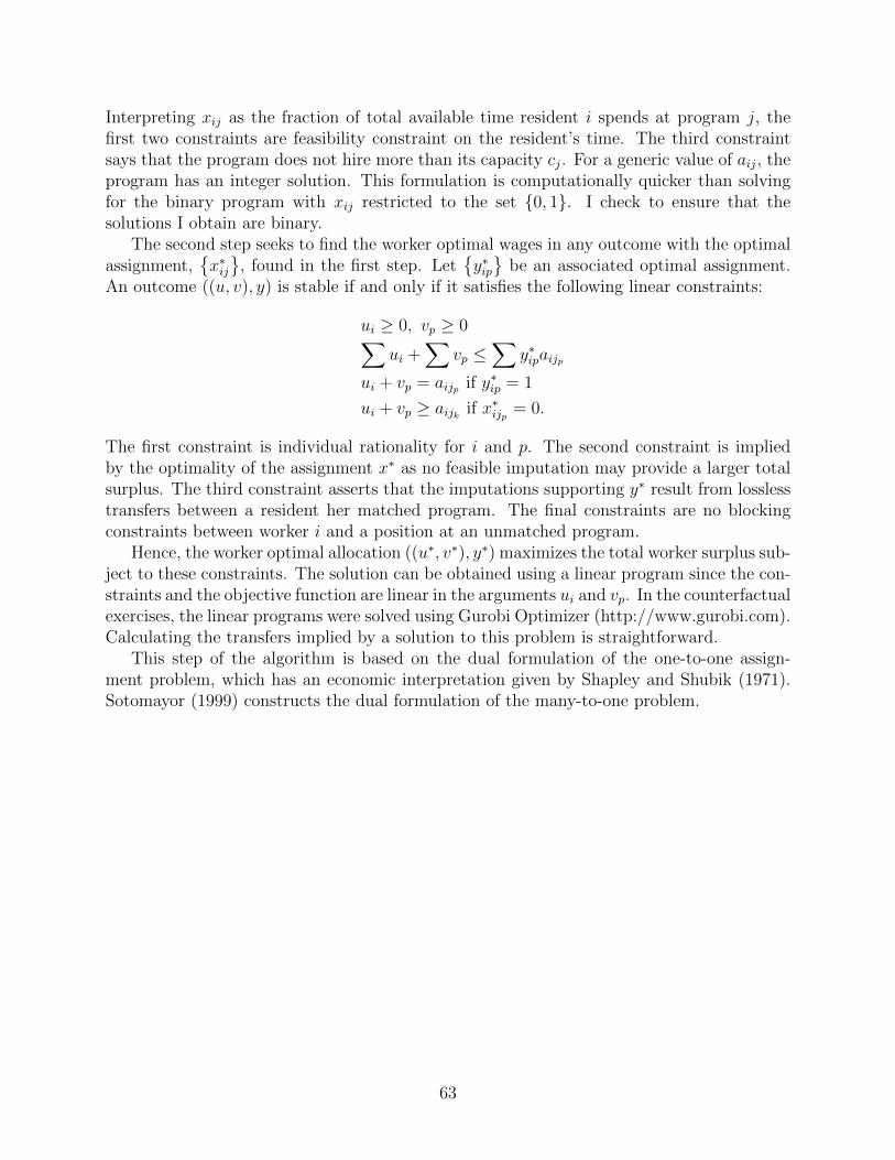
Interpreting xij as the fraction of total available time resident i spends at program j, thefirst two constraints are feasibility constraint on the resident’s time. The third constraintsays that the program does not hire more than its capacity cj. For a generic value of aij, theprogram has an integer solution. This formulation is computationally quicker than solvingfor the binary program with xij restricted to the set {0, 1}. I check to ensure that thesolutions I obtain are binary.

The second step seeks to find the worker optimal wages in any outcome with the optimalassignment,

{x∗ij}

, found in the first step. Let{y∗ip}

be an associated optimal assignment.An outcome ((u, v), y) is stable if and only if it satisfies the following linear constraints:

ui ≥ 0, vp ≥ 0∑ui +

∑vp ≤

∑y∗ipaijp

ui + vp = aijp if y∗ip = 1

ui + vp ≥ aijk if x∗ijp = 0.

The first constraint is individual rationality for i and p. The second constraint is impliedby the optimality of the assignment x∗ as no feasible imputation may provide a larger totalsurplus. The third constraint asserts that the imputations supporting y∗ result from losslesstransfers between a resident her matched program. The final constraints are no blockingconstraints between worker i and a position at an unmatched program.

Hence, the worker optimal allocation ((u∗, v∗), y∗) maximizes the total worker surplus sub-ject to these constraints. The solution can be obtained using a linear program since the con-straints and the objective function are linear in the arguments ui and vp. In the counterfactualexercises, the linear programs were solved using Gurobi Optimizer (http://www.gurobi.com).Calculating the transfers implied by a solution to this problem is straightforward.

This step of the algorithm is based on the dual formulation of the one-to-one assign-ment problem, which has an economic interpretation given by Shapley and Shubik (1971).Sotomayor (1999) constructs the dual formulation of the many-to-one problem.

63