An Empirical Model of Price Competition with Predatory

An Empirical Model of Price Competition with Predatory

Strategies and Network Effects, with an Application to the

Mexican Wireless Telecommunications Market

Andres Aradillas-Lopez∗

December 7, 2020

Abstract

We present an oligopolistic model of price competition where one player has an

additional non-price “predatory strategy” that can shift consumer preferences away

from its competitors. This strategy is treated as an unobserved market-level random

variable which is optimally chosen in equilibrium, along with prices, in a noncooperative

game. We also include a “network effect” whereby consumer preferences depend on their

beliefs about the proportion of consumers that will choose each one of the competing

players. Ours is a special case of a BLP-style demand model with a market-level,

firm-specific unobserved shock in consumers’ utility that is explicitly modeled as a

function of the unobserved predatory strategy. We apply our model to the Mexican

wireless telecommunications industry where three carriers serve the market and where

the dominant player (America Movil or ‘AMX’) has had a market share consistently

above 60% in spite of reforms enacted in 2013 to promote competition. Our example

is suitable since AMX has engaged in documented practices that fit our description

of predatory strategies. Our results suggest that, while the network effect has lost

significance over time to explain AMX’s market share, the predatory-strategy effect has

increased in magnitude. This finding has important policy implications.

JEL Codes: C3, C51, C57, D12, L10.

1 Introduction

We present an oligopolistic model of price competition where one of the competing firms

has at its disposal an additional non-price strategy that can shift consumers’ preferences

away from its competitors and towards itself. We call this a predatory strategy and it

∗email: [email protected]. Pennsylvania State University. Department of Economics, 518 Kern GraduateBuilding, University Park, PA 16802

1

is meant to summarize all the non-price practices that this player can undertake which

have the aforementioned ability of pulling consumers away from its competitors. These

practices are not necessarily anticompetitive in nature, although our empirical example

will deal with an industry (the Mexican wireless phone market) where the dominant firm,

America Movil (AMX), has engaged in documented anticompetitive behavior consistent

with the characterization of predatory strategy in our model. The model will also include a

network effect whereby each consumer’s preferences depend on her expectations about the

proportion of consumers who will select each firm.

Our baseline model is motivated by the real-world features of our empirical example:

the Mexican wireless telecommunications industry. Accordingly, the first feature of our

model is that it will involve three competing firms: a dominant firm with the ability of

using a predatory strategy, and two other firms whose only strategy is price. The second

main feature is that we will assume that the researcher only has market-level data (not

individual consumer data). The predatory strategy will be treated as an unobserved market-

level random variable which is chosen optimally, along with prices, as the equilibrium of

a noncooperative game. Our model will enable us to separate the network effect from

the predatory effect in order to explain market shares. This is a policy-relevant question

in our empirical example and potentially in many other real-world applications. Even

though the features of our baseline model are tailored to fit our application, we discuss

several extensions, such as having more players and alternative specifications for consumer

preferences.

In the context of models of consumer behavior, ours can be seen as a special case

of BLP demand models (Berry, Levinsohn, and Pakes (1995)) with an unobserved, firm-

specific, market-level shock in consumers’ utility functions which is modeled explicitly as a

function of the unobserved predatory strategy. To our knowledge, this is the first BLP-type

demand model of price competition that also includes a non-price predatory strategy and

a network effect. The paper proceeds as follows. Section 2 describes our baseline model.

Section 3 describes the type of data we assume and the observable implications from our

model. Extensions of the baseline model are discussed in Section 4. Our empirical example

is presented in Section 5 and Section 6 concludes

2 Model

2.1 Players’ strategies

We have three players1: j ∈ {1, 2, 3}, who provide a differentiated good or service. They

compete against each other in order to attract consumers in market t. Based on the features

1We will choose the term “player” and “firm” interchangeably.

2

of our empirical example, our setup is one where the same three firms compete against each

other repeatedly in a collection of markets t = 1, . . . , T , and these are the only firms

consumers can select to receive the good or service in question. Also motivated by our

empirical example we will focus on a situation where we have data at the market level (not

at the individual consumer level). Extensions to more than 3 players as well as the case

where consumer-level data is available will be discussed in Section 4.

2.1.1 Prices

The three firms choose prices in market t, labeled as p1t, p2t and p3t.

2.1.2 Predatory strategy of player 1

In addition to the price p1t, player 1 also has a predatory strategy, labeled as at which can

shift the preferences of consumers and “separate” them from players 2 and 3 (in a way to be

described below) and towards player 1. We think about at as an aggregate measure of the

non-price predatory practices undertaken by player 1 and we assume at ∈ [0,∞), with at = 0

representing the case where there are no predatory efforts exerted by player 1 in market

t. Empirical examples of non-price predatory strategies and tactics are described in Gund-

lach (1990). Among the ones mentioned there which can fit the description of “predatory

strategy” in our model (see equation (2.1) below) are the following: predatory advertising

(dispariging advertising or promotional activities beyond those required to maintain brand

recognition), market channel exclusionary covenants (contractual terms with suppliers or

outlets that preclude them from dealing with rivals), market channel integration (using

ownership of essential inputs, infrastructure or sales/distribution networks to strategically

shift consumers away from its rivals), among others. Predatory practices do not necessarily

involve anticompetitive behavior. However, some of the documented predatory strategies of

the dominant player (AMX) in our empirical example include documented anticompetitive

practices which we will describe in Section 5.

2.2 Consumers

Inspired by the features of our empirical example, we will focus on a situation where we

have data at the market level (not at the individual consumer level), and this will inform

our assumptions and modeling choices for our baseline model2. Our first assumption is that

we have a population of Nt symmetric consumers in market t. The ith consumer in market

2Section 4 will discuss several extensions.

3

t has random utilities given as follows,

Vi1t = ∆1 − β1 · p1t + σ1 · at + λt · πei1t + ξi1t, (utility of choosing firm 1)

Vi2t = ∆2 − β2 · p2t − σ2 · at + λt · πei2t + ξi2t, (utility of choosing firm 2)

Vi3t = ∆3 − β3 · p3t − σ3 · at + λt · πei3t + ξi3t, (utility of choosing firm 3)

(2.1)

Where πeijt denotes consumer i’s subjective expectation (beliefs) for the proportion of con-

sumers in market t that will choose firm j. Since we assume that these three firms are

the only alternatives for consumers3, beliefs must satisfy πei1t + πei2t + πei3t = 1, and we can

rewrite Vi3t as

Vi3t = ∆3 − β3 · p3t − σ3 · at + λt · (1− πei1t − πei2t) + ξi3t.

ξijt is a privately observed, idiosyncratic random utility shock, unobserved by firms or by

the econometrician, while ∆j , βj , σ2, σ3 and λt are unknown parameters. Note that λt is

explicitly allowed to change across markets. We will treat it as an unobserved market-level

random coefficient. Note from (2.1) that preferences depend on the following:

• Prices.

• The expected proportion of the market that will choose each firm. This represents

what we will call the network effect.

• The predatory strategy of firm 1.

• A random utility component which represents consumers’ idiosyncratic preferences

for each of the three firms.

The parameter βj measures the direct effect of price pjt on the utility of choosing firm j,

while λt measures the network effect in market t. The parameters σ1, σ2 and σ3 measure

the effect of the predatory strategy at on consumers’ preferences. If we assumed that the

network effect is positive, the expected signs for the preference parameters in (2.1) would

be

βj ≥ 0, σ1 ≥ 0, σ2 ≥ 0, σ3 ≥ 0, λt ≥ 0

If σ1 = σ2 = σ3 = 0, the predatory actions of firm 1 have no effect on consumer preferences.

Allowing for σ2 6= σ3 allows for different effects of firm 1’s predatory strategy on each of its

competitors.

The effect of at on preferences described in (2.1) fully captures the impact of what we

call the “predatory strategy” of player 1 in this paper. Mathematically, it provides player

3The model can be straightforwardly extended to include an outside option in the usual way.

4

1 the ability of shifting consumer preferences, away from players 2 and 3, and towards

herself. Beyond this, our model is not specific about what exactly constitutes the extent of

the predatory practices. However, we will enumerate a list of documented practices in our

empirical example and we will explain there why the type of shift in preferences described

in (2.1) is a reasonable approximation.

Advertising is perhaps the main example of non-price predatory strategies studied pre-

viously in oligopolistic models. In this literature a distinction has been made between

predatory advertising and cooperative advertising. The difference lies in the type of ex-

ternalities generated by it. While cooperative advertising results in positive externalities

that expand the market for all firms, predatory advertising produces negative externali-

ties that merely redistribute market shares (see Chen, Roayaei, and Seldon (1993)). The

latter is the type of effect described in (2.1). To our knowledge, this paper presents the

first empirically-oriented model of consumer choice that models explicitly price competition

alongside a predatory strategy.

Assumption 1 The random utility shocks (ξi1t, ξi2t, ξi3t) are independent of beliefs πeijt,

market prices pjt and the predatory strategy at. These utility shocks are iid with a Type I

Extreme Value distribution and their realization is only privately observed by each consumer.

Let pt ≡ (p1t, p2t, p3t). Take any given pair π1, π2 ∈ [0, 1]2 such that π1 + π2 ≤ 1 and let

π ≡ (π1, π2). Define,

G1t(pt, at, π) =e∆1−β1·p1t+σ1·at+λt·π1

e∆1−β1·p1t+σ1·at+λt·π1 + e∆2−β2·p2t−σ2·at+λt·π2 + e∆3−β3·p3t−σ3·at+λt·(1−π1−π2),

G2t(pt, at, π) =e∆2−β2·p2t−σ2·at+λ·π2

e∆1−β1·p1t+σ1·at+λt·π1 + e∆2−β2·p2t−σ2·at+λt·π2 + e∆3−β3·p3t−σ3·at+λt·(1−π1−π2),

G3t(pt, at, π) = 1−G1t(pt, at, π)−G2t(pt, at, π).

(2.2)

Let πeit ≡ (πei1t, πei2t). From Assumption 1 we have,

Pr [Consumer i chooses firm j in market t|pt, at, πeit] = Gjt(pt, at, πeit)

Conditional on payoff parameters, beliefs, prices and on the predatory strategy, ours is a

characteristics-based demand model with Logit choice probabilities (see McFadden (1974)

and Nevo (2011, Section 3.3.2)).

5

2.2.1 Reparameterization

Define γ2 ≡ σ1 + σ2, γ3 ≡ σ1 + σ3, δ2 ≡ ∆2 −∆1 and δ3 ≡ ∆3 −∆1. Group

θ ≡ (δ2, δ3, β1, β2, β3, γ2, γ3) ∈ R7. (2.3)

The probabilities in (2.2) can be written as

G1(pt, at, π|θ, λt) ≡e−β1·p1t+λt·π1

e−β1·p1t+λt·π1 + eδ2−β2·p2t−γ2·at+λt·π2 + eδ3−β3·p3t−γ3·at+λt·(1−π1−π2),

G2(pt, at, π|θ, λt) =eδ2−β2·p2t−γ2·at+λt·π2

e−β1·p1t+λt·π1 + eδ2−β2·p2t−γ2·at+λt·π2 + eδ3−β3·p3t−γ3·at+λt·(1−π1−π2),

G3(pt, at, π|θ, λt) = 1−G1(pt, at, π|θ, λt)−G2(pt, at, π|θ, λt)(2.4)

Note that

Pr [Consumer i chooses firm j in market t|pt, at, πeit] = Gj(pt, at, πeit|θ, λt).

The model is therefore observationally equivalent to one where random utility functions are

given by

Vi1t = −β1 · p1t + λt · πei1t + ξi1t,

Vi2t = δ2 − β2 · p2t − γ2 · at + λt · πei2t + ξi2t,

Vi3t = δ3 − β3 · p3t − γ3 · at + λt · (1− πei1t − πei2t) + ξi3t.

(2.5)

We assume individual consumer beliefs are unobserved in the data. In order to recover them,

we will impose the assumption that every consumer holds equilibrium beliefs as described

next.

2.2.2 Equilibrium beliefs

Assumption 2 For a given θ and a given (p, a, λ), we refer to equilibrium beliefs as any

pair π1, π2 ∈ [0, 1]2 with π1 + π2 ≤ 1 that solve the system

π1 −G1(p, a, π|θ, λ) = 0

π2 −G2(p, a, π|θ, λ) = 0(2.6)

We assume that, given the prices and predatory strategies chosen by the firms, consumers

hold equilibrium beliefs and, if the equilibrium system (2.6) has multiple solutions, consumers

6

use the same, degenerate equilibrium selection rule to choose one solution w.p.1. That is,

their equilibrium selection rule does not randomize across existing solutions. Note that this

implies that consumers’ beliefs correspond to firms’ true ex-post market shares.

Existence of a solution to (2.6) follows from Brouwer’s fixed-point theorem (de la Fuente

(2000, Chapter 5, Theorem 3.2)). Sufficient conditions for uniqueness can be characterized

in terms of properties of the principal minors of the Jacobian of (2.6) with respect to π, as

in Gale and Nikaido (1965).

Assumption 2 and the existence of a representative consumer

Under Assumption 2 we have πit = πt for all i = 1, . . .Nt, where πt satisfy (2.6). There-

fore every consumer’s choice probabilities correspond to those of a representative consumer

whose choices are summarized as,

Pr [Representative consumer chooses firm j in market t|pt, at, πeit] = Gj(pt, at, πt|θ, λt).

The model of consumer behavior we have assumed so far is a special case of the class of

demand models in the “product characteristics space” described in Nevo (2011, Section

3.3.2). By treating both the network-effect coefficient λt and the predatory strategy at as

unobserved market-level random variables, ours will be a special case of the family of BLP

demand models (Berry, Levinsohn, and Pakes (1995)) which use random coefficients and

introduce unobserved product-specific characteristics in consumers’ random utility func-

tions. What is special about our model is that it adds structure to these product-specific

(in our case, firm-specific) characteristics by modeling them as functions of the unobserved

predatory strategy at. Like BLP models, we will use equilibrium conditions to recover the

unobserved at and λt. We describe firms’ optimal choice of prices and of the predatory

strategy next.

2.3 Firms’ expected payoffs

Now we will describe firms’ choice of prices and of the predatory strategy. In order to do this

we need to characterize their expected payoffs, which requires specifying our assumptions

about firms’ costs, the sequence of moves, and the information possessed by firms when

they choose their strategies.

2.3.1 Costs of providing service

We assume that each firm j has a constant cost-per-consumer of providing the good or

service in market t and we denote it as cjt. For each consumer in the market, firm j

7

incurs this cost if and only if it provides the good or service to the consumer. Thus the

revenue-per-consumer for firm j is pjt − cjt. We assume that the realization of (c1t, c2t, c3t)

is common knowledge among the firms prior to making their choices.

2.3.2 Predatory strategy costs

Firm 1 has a cost associated with the predatory strategy. We assume that this cost is only

a function of the level chosen for at and is independent of the number of consumers in the

market that select firm 1. We denote this cost as ca(at) and, for simplicity, we assume that

the cost function ca(·) is the same across all markets, but this could be relaxed. The cost

function ca(·) is assumed to be common knowledge among the three firms.

2.3.3 Firms’ information about consumers

Next we specify the information firms are assumed to possess about consumer behavior.

Assumption 3 Firms are unable to observe the characteristics of each consumer in the

market prior to choosing their strategies. We assume that the following information is

common knowledge among firms in each market t,

• The distribution of the idiosyncratic utility shocks ξijt as described in Assumption 1.

• The true value of the utility parameters θ and the realization of the network-effect

coefficient λt.

• The fact that consumers’ beliefs satisfy the equilibrium conditions in (2.6).

• The number of consumers Nt.

2.3.4 Sequence of choices and firms’ expected payoffs

Firms first choose their strategies (prices and the predatory strategy) simultaneously and,

once these are set, consumers make their choices. Letting

Yijt = 1 { consumer i selects firm j in market t} ,

8

firms’ ex-post payoffs are

u1t = (p1t − c1t) ·Nt∑i=1

Yi1t − ca(at),

u2t = (p2t − c2t) ·Nt∑i=1

Yi2t,

u3t = (p3t − c3t) ·Nt∑i=1

Yi3t.

However, due to the sequence of moves, firms must choose their strategies prior to observing

consumers’ choices, so they must focus on the ex-ante expected payoffs. Fix p ≡ (p1, p2, p3)

and a. By Assumption 3, firms’ expected payoffs in market t if pt = p and at = a are given

by

E [u1t|pt = p, at = a] = Nt ·(

(p1 − c1t) ·G1(p, a, πe|θ, λt)−ca(a)

Nt

),

E [u2t|pt = p, at = a] = Nt ·(

(p2 − c2t) ·G2(p, a, πe|θ, λt)),

E [u3t|pt = p, at = a] = Nt ·(

(p3 − c3t) ·[1−G1(p, a, πe|θ, λt)−G2(p, a, πe|θ, λt)

]),

Where πe are the beliefs of the representative consumer given p and a. By Assumption 3,

firms recover πe as the solution to the equilibrium system (2.6) for the given p and a. From

the above expressions, in choosing their optimal strategies firms can focus on maximizing

the expected payoff-per-consumer in the market,

u1(p, a, πe|θ, λt, c1t, ca,Nt) ≡ (p1 − c1t) ·G1(p, a, πe|θ, λt)−ca(a)

Nt,

u2(p, a, πe|θ, λt, c2t) ≡ (p2 − c2t) ·G2(p, a, πe|θ, λt),

u3(p, a, πe|θ, λt, c3t) ≡ (p3 − c3t) · [1−G1(p, a, πe|θ, λt)−G2(p, a, πe|θ, λt)] .

(2.7)

2.4 Equilibrium strategies

By Assumption 3, firms internalize the fact that the representative consumer’s beliefs solve

the equilibrium system (2.6). We take advantage of this assumption by expressing the

unobserved market-level network effect λt and the unobserved predatory strategy at as

implicit functions of prices and market shares by solving (2.6).

9

2.4.1 Network effect, predatory strategy and Assumption 3

We have assumed that the conditions in Assumption 3 are common knowledge among the

competing firms and that this is internalized into their optimal strategy choices. Thus, in

equilibrium, the network effect λt and the predatory strategy at can be defined implicitly as

functions of prices p and market shares π since they must solve the system given in (2.6).

Accordingly, for a given set of prices and market shares (p, π) and given θ, we will denote

the solutions in (λ, a) to the equilibrium-belief system (2.6) as λ(p, π|θ) and a(p, π|θ). For a

pre-specified set of market shares π, plugging in these solutions into firms’ expected payoff

functions will allow us to characterize the equilibrium of the game purely in terms of prices

p. This will be helpful when bringing the model to the data, where we will plug-in the

observed market shares πt in each market t.

Recovering λ and a by solving (2.6) is the same principle used in BLP models (Berry,

Levinsohn, and Pakes (1995)) to recover unobserved product-specific characteristics in de-

mand models (see Nevo (2011)). In the context of BLP models, ours can be seen as a special

case in which these unobserved product characteristics are modeled explicitly as functions

of the unobserved predatory strategy. Sufficient conditions for invertibility of (2.6) can be

based on properties of the principal minors of its Jacobian (with respect to λ and a), as

described in Gale and Nikaido (1965). They can also be based on the results presented in

Berry, Haile, and Gandhi (2013).

2.4.2 Best-response prices

Expressing the network effect and the predatory strategy as implicit functions of prices and

market shares by solving (2.6) allows us in turn to express expected payoff functions solely

as functions of prices for a given set of market shares. For a pre-specified π and a given p,

let us replace λ and a with λ(p, π|θ) and a(p, π|θ) respectively in the expressions of expected

payoff functions (2.7). We obtain,

u1(p, π|θ, c1t, ca,Nt) = (p1 − c1t) ·G1(p, a(p, π|θ), π|θ, λ(p, π|θ))− ca(a(p, π|θ))Nt

,

u2(p, π|θ, c2t) = (p2 − c2t) ·G2(p, a(p, π|θ), π|θ, λ(p, π|θ)),

u3(p, π|θ, c3t) = (p3 − c3t) · [1−G1(p, a(p, π|θ), π|θ, λ(p, π|θ))−G2(p, a(p, π|θ), π|θ, λ(p, π|θ))] .(2.8)

This is useful because, for a given set of market shares π, the equilibrium can be described

entirely in terms of prices p.

Fix a set of market shares π. For a given c1, ca and N , let BR1(p2, p3, π|θ, c1, ca,N )

denote the best-response price p1 for firm 1 if its opponents choose prices p2, p3. Similarly,

for a given c2 let BR2(p1, p3, π|θ, c2) denote the best-response price p2 for firm 2 if its

10

opponents choose prices p1, p3. Finally, for a given c3 let BR3(p1, p2, π|θ, c3) denote the

best-response price p3 for firm 3 if its opponents choose prices p1, p2. We have

BR1(p2, p3, π|θ, c1, ca,N ) = argmaxp1≥0

{u1(p, π|θ, c1, ca,N )

},

BR2(p1, p3, π|θ, c2) = argmaxp2≥0

{u2(p, π|θ, c2)

},


{u3(p, π|θ, c3)

}.

(2.9)

3 Data and observable implications

We assume to observe t = 1, . . . , T realizations of this game, each one called a “market”. For

the tth realization of the game, the researcher observes prices pt ≡ (p1t, p2t, p3t), a measure

of service costs ct ≡ (c1t, c2t, c3t) and market shares πt ≡ (π1t, π2t) (with π3t = 1−π1t−π2t).

With regard to Nt (the size of the market) we assume that either of the following is true,

(a) Nt is known for all t, or

(b) Nt/Nt∗ is known for all t and some t∗.

Case (b) will correspond to our empirical example.

3.1 Treating observed prices as best-response equilibrium prices given

the observed market shares

Suppose the prices observed pt correspond to an equilibrium of the game given the observed

market shares πt and costs ct ≡ (c1t, c2t, c3t). Then the following must be true. For a given

price vector p ≡ (p1, p2, p3) take the best-responses

BR1(p2, p3, πt|θ, c1t, ca,Nt) = argmaxp1≥0

{(p1 − c1t) ·G1

(p, a(p, πt|θ), πt

∣∣θ, λ(p, πt|θ))− ca (a(p, πt|θ))

Nt

},

BR2(p1, p3, πt|θ, c2t) = argmaxp2≥0

{(p2 − c2t) ·G2(p, a(p, πt|θ), πt|θ, λ(p, πt|θ))

},



}.

(3.1)

If we assume that the prices observed constitute an equilibrium of the game, then

p1t = BR1(p2t, p3t, πt|θ, c1t, ca,Nt),

p2t = BR2(p1t, p3t, πt|θ, c2t),

p3t = BR3(p1t, p2t, πt|θ, c3t).

(3.2)

11

The restrictions in (3.6) would summarize the observable implications of our model and

they would be the basis for inference. In order to proceed we must make more precise

assumptions about the predatory-strategy cost function ca.

3.2 A specification for the cost function of the predatory strategy, cacaca

Using (3.6) to infer θ requires assumptions about ca, the cost function for the predatory

strategy a. As an illustration suppose we assume a power cost function of the form,

ca(a) = ζa · ar.

We assume ζa > 0 to be a parameter that is constant across all markets t = 1, . . . , T and

r > 0 is a pre-specified power. Consistent with our assumptions about what the researcher

observes about Nt, let t∗ be a market for which Nt/Nt∗ ≡ ηt is known for all t. Define

κa ≡ζaNt∗

, and let a ≡ κa1/r · a.

Then, the cost-per-consumer of the predatory strategy a is

ca(a)

Nt=

1

ηt· ar

The parameter κa cannot be separately identified from the random utility coefficients γ2

and γ3 which measure the sensitivity of consumers’ preferences to the predatory strategy

a (see Equation (2.5)). To see why, let γ2 ≡ γ2/κa1/r and γ3 ≡ γ3/κa

1/r. Then we could

re-express the entire model in terms of at ≡ κa1/r ·at. The random utility functions in (2.5)

can be expressed as

Vi1t = −β1 · p1t + λ · πei1t + ξi1t,


Vi3t = δ3 − β3 · p3t − γ3 · at + λt · (1− πei1t − πei2t) + ξi3t.

Accordingly, the choice probabilities of the representative consumer would be computed

from here replacing (γ2, γ3) with (γ2, γ3) and a with a. Finally, firms’ expected payoffs-per-

consumer in market t can be expressed as

u1(p, a, πe|θ, λ, c1, ηt) = (p1 − c1) ·G1(p, a, πe|θ, λ)− 1

ηt· ar,

u2(p, a, πe|θ, λ, c2) = (p2 − c2) ·G2(p, a, πe|θ, λ),

u3(p, a, πe|θ, λ, c3) = (p3 − c3) · [1−G1(p, a, πe|θ, λ)−G2(p, a, πe|θ, λ)] .

12

Thus, any cost function of the form ca(a) = ζa · ar is observationally equivalent to a model

where the cost-per-consumer for the predatory strategy is

1

ηt· ar (3.3)

and where the predatory-strategy sensitivity parameters in (2.5) are measured relative to

κa1/r ≡ ζa/Nt∗1/r. As a result, we shall assume the cost-per-consumer expression (3.3)

and our interpretation for the magnitude of the parameters γ2, γ3 will be relative to κa1/r.

As a result, under this specification for predatory-strategy costs, our expected payoff-per-

consumer functions in market t described in (2.7) become,

u1(p, a, πe|θ, λt, c1t, ηt) ≡ (p1 − c1t) ·G1(p, a, πe|θ, λt)−1

ηt· ar,

u2(p, a, πe|θ, λt, c2t) ≡ (p2 − c2t) ·G2(p, a, πe|θ, λt),

u3(p, a, πe|θ, λt, c3t) ≡ (p3 − c3t) · [1−G1(p, a, πe|θ, λt)−G2(p, a, πe|θ, λt)] .

(3.4)

3.3 Observable implications for θ

Using the power function specification for predatory-strategy costs described in Section

3.2 and the resulting expression for expected payoff-per-consumer functions in (3.4), the

best-response functions described in (3.1) become,

BR1(p2, p3, πt|θ, c1t, ηt) = argmaxp1≥0

{(p1 − c1t) ·G1

(p, a(p, πt|θ), πt

∣∣θ, λ(p, πt|θ))− 1

ηt· a(p, πt|θ)r

},



},



}.

(3.5)

If we assume that the prices observed constitute an equilibrium of the game, then

p1t = BR1(p2t, p3t, πt|θ, c1t, ηt),



(3.6)

The equilibrium relationship between prices and best-response functions described in (3.6)

summarizes the observable implications of the model and would therefore lay the inferential

foundation for θ. A generic moment-based approach can be described as follows. Group

BR(pt, πt|θ, ct, ηt) ≡(BR1(p2t, p3t, πt|θ, c1t, ηt), BR2(p1t, p3t, πt|θ, c2t), BR3(p1t, p2t, πt|θ, c3t)

)′.

13

Let zt denote additional observable variables (if any) other than (pt, ct, πt, ηt) and let xt ≡(pt, ct, πt, ηt, zt). Take a function

ρ(pt −BR(pt, πt|θ, ct, ηt);xt) such that E [ρ(0;xt)] = 0.

For example,

ρ(pt −BR(pt, πt|θ, ct, ηt);xt) = Σ(xt) (pt −BR(pt, πt|θ, ct, ηt)) ,

where Σ(xt)︸︷︷︸d×3

is a prespecified collection of “instrument functions”. Let

M(θ) = E [ρ(pt −BR(pt, πt|θ, ct, ηt);xt)] ,

where the expectation is taken over the observable characteristics xt ≡ (pt, ct, πt, ηt, zt).

Our assumptions imply that, for any such ρ, we must have

M(θ) = 0. (3.7)

Estimation and inference (e.g, the construction of a confidence set) for θ can be based

on (3.7) employing conventional moment-based econometric methods (see Newey and Mc-

Fadden (1994)). Alternatively, a more powerful approach based on conditional moment

restrictions can be employed (see, e.g, Dominguez and Lobato (2004) and Andrews and Shi

(2013)).

4 Extensions

Our baseline model is inspired by the features of our eventual empirical example. However,

the model can be extended in multiple ways depending on the richness of the data. We

outline some of the most important potential extensions here.

4.1 A model with J ≥ 4J ≥ 4J ≥ 4 competing firms

The most straightforward extension would be to leave player 1 as the only one with a

predatory strategy but extend the setting from 3 to J ≥ 4 total players, J − 1 of which can

be affected by the predatory efforts of player 1. To be precise, suppose we generalize the

14

random utility system (2.5) to

Vi1t = −β1 · p1t + λt · πei1t + ξi1t,




......

......

......

...

ViJt = δJ − βJ · pJt − γJ · at + λt ·

1−J−1∑j=1

πeijt

+ ξiJt

(4.1)

Generalizing Assumption 1 to this case, (ξi1t, ξi2t, . . . , ξiJt) would be assumed to be iid with

a Type I Extreme Value distribution and the choice probability expressions in (2.4) would

be straightforwardly extended to G1(pt, at, π|θ, λt), G2(pt, at, π|θ, λt), . . ., GJ(pt, at, π|θ, λt)in this case. If we generalize the equilibrium-beliefs conditions in Assumption 2, the system

(2.6) would become

π1 −G1(p, a, π|θ, λ) = 0,

π2 −G2(p, a, π|θ, λ) = 0,

π3 −G3(p, a, π|θ, λ) = 0,

......

......

...

πJ−1 −GJ−1(p, a, π|θ, λ) = 0.

J − 1 restrictions (4.2)

In our 3-player model we used the equilibrium-belief system (4.2) to express λ and a as

implicit functions of prices p and market shares π. We can extend this approach as follows.

Partition prices as

p ≡ (p1, p2, p3︸︷︷︸≡pI

, p4, . . . , pJ︸︷︷︸≡pII

) ≡ (pI , pII), where pI ≡ (p1, p2, p3), pII ≡ (p4, . . . , pJ).

Suppose we assume again the power function specification for the predatory strategy cost

function described in Section 3.2. Using (4.2), we can now express (λ, a, pII) ∈ RJ−1 as

implicit functions of (pI , π). Denoting them as λ(pI , π|θ), a(pI , π|θ) and pII(pI , π|θ) and

letting

p(pI , π|θ) ≡ (pI , pII(pI , π|θ)),

15

the equilibrium expected payoff functions of firms 1, 2 and 3 can be expressed as

u1(pI , π|θ, c1, η) = (p1 − c1) ·G1(p(pI , π|θ), a(pI , π|θ), π|θ, λ(pI , π|θ))− a(pI , π|θ)r

η,

u2(pI , π|θ, c2) = (p2 − c2) ·G2(p(pI , π|θ), a(pI , π|θ), π|θ, λ(pI , π|θ)),

u3(pI , π|θ, c3) = (p3 − c3) ·G3(p(pI , π|θ), a(pI , π|θ), π|θ, λ(pI , π|θ)).

(4.3)

This is a generalization of (2.8). Best-response prices for firms 1,2 and 3 are given by

BR1(p2, p3, π|θ, c1, η) = argmaxp1≥0

{u1(pI , π|θ, c1, η)

},


{u2(pI , π|θ, c2)

},


{u3(pI , π|θ, c3)

}.

(4.4)

This is a generalization of equation (2.9). As it was the case with J = 3 and equation (3.6),

if we assume that prices observed are equilibrium prices, the implications of the model

would be summarized by the conditions

p1t = BR1(p2t, p3t, πt|θ, c1t, ηt),



(4.5)

Inference for θ can then proceed using the arguments outlined in Section 3.3. Note that

when J ≥ 4 we can follow the previous steps with any combination of 3 out of the J

competing firms as the elements in pI (i.e, not necessarily firms 1, 2 and 3). In this sense

the model would now be overidentified.

4.2 Allowing for firm-specific, market-level random utility coefficients δjtδjtδjt

Let us remain in the more general J ≥ 4 player setting. A key feature of BLP demand

models is the inclusion of market-level, product-specific unobserved random utility shocks.

We can enrich our model in this fashion by allowing the firm-specific utility shocks δj to be

market-level, unobserved random variables. Accordingly, let us denote them now as δjt, for

j = 2, . . . , J .

One way to approach this could be as follows. Let us now assume that the network

16

coefficient λ is constant across all markets4. Group

δ ≡ (δ2, δ3, . . . , δJ), Γ ≡ (β1, β2, . . . , βJ , γ2, γ3, . . . , γJ , λ).

Accordingly, for a given (p, a, π, δ,Γ) let us express the choice probabilities as Gj(p, a, π|δ,Γ).

The belief-equilibrium system (4.2) can be expressed as

π1 −G1(p, a, π|δ,Γ) = 0,

π2 −G2(p, a, π|δ,Γ) = 0,

π3 −G3(p, a, π|δ,Γ) = 0,

......

......

...

πJ−1 −GJ−1(p, a, π|δ,Γ) = 0.

J − 1 restrictions (4.6)

For a given (p, a, π,Γ), we can now use the equilibrium-belief system (4.6) to recover δ as

an implicit function of (p, a, π,Γ). Let us denote it as

δ(p, a, π,Γ) ∈ RJ−1 (4.7)

Conditions for the system (4.6) to be invertible in terms of δ is the type of problem studied

in Berry, Haile, and Gandhi (2013). Again, sufficient conditions can revolve around the

principal minor properties of the Jacobian of (4.6) (with respect to δ) described in Gale

and Nikaido (1965). Let us maintain the power-function specification for the predatory

strategy cost we analyzed above. For a given (p, a, π,Γ), we can plug in (4.7) in place of δ

and obtain an expression for expected payoff-per-consumer functions in terms of (p, a, π,Γ)

along with the costs (c1, c2, . . . , cJ) and η

u1(p, a, π|Γ, c1, η) = (p1 − c1) ·G1

(p, a, π

∣∣δ(p, a, π,Γ),Γ)− ar

η,

u2(p, a, π|Γ, c2) = (p2 − c2) ·G2

(p, a, π

∣∣δ(p, a, π,Γ),Γ),

......

......

......

......

...

uJ(p, a, π|Γ, cJ) = (pJ − cJ) ·GJ(p, a, π

∣∣δ(p, a, π,Γ),Γ).

For a given (p, π,Γ, c1, η), the optimal choice for the predatory strategy of firm 1 is given

by,

a∗(p, π|Γ, c1, η) = argmaxa≥0

{u1(p, a, π|Γ, c1, η)} .

4Instead of using this assumption, we could impose a restriction –e.g, symmetry– that reduces the di-mensionality of the unknown market-specific coefficients δjt’s below J − 1.

17

Let us now plug in this expression in place of a in the expected payoff functions described

above, so we can express them solely as functions of (p, π,Γ, c1, . . . , cJ , η),

u1(p, π|Γ, c1, η) ≡ u1

(p, a∗(p, π|Γ, c1, η), π|Γ, c1, η

),

u2(p, a, π|Γ, c2, c1, η) ≡ u2(p, a∗(p, π|Γ, c1, η), π|Γ, c2),

......

......

......

......

...

uJ(p, a, π|Γ, cJ , c1, η) ≡ uJ(p, a∗(p, π|Γ, c1, η), π|Γ, cJ).

Let p−j ≡ (p`) 6=j . From the above expressions we can characterize best-response prices for

each firm,

BR1(p−1, π|Γ, c1, η) = argmaxp1≥0

{u1(p, π|Γ, c1, η)} ,

BR2(p−2, π|Γ, c2, c1, η) = argmaxp2≥0

{u2(p, a, π|Γ, c2, c1, η)} ,

......

......

......

......

...

BRJ(p−J , π|Γ, cJ , c1, η) = argmaxpJ≥0

{uJ(p, a, π|Γ, cJ , c1, η)} .

From here, if we assume that the prices observed in market t are an equilibrium, the

implications of the model would be summarized by the conditions

p1t = BR1(p−1t, πt|Γ, c1t, ηt),

p2t = BR2(p−2t, πt|Γ, c2t, c1t, ηt),

......

......

......

pJt = BRJ(p−Jt, πt|Γ, cJt, c1t, ηt).

(4.8)

Inference for Γ can proceed from here along the lines of Section 3.3.

4.3 Introducing consumer-level data

Our baseline model presupposed that we only have market-level data. Adapting it to

consumer-level data can be done straightforwardly, as it is the case in BLP-type demand

models (see Nevo (2000) and Nevo (2011, Section 3.3.2)). For example, this can allow us to

assume random-coefficients at the individual level for consumers’ random utility functions

which can be parameterized as functions of observable consumer characteristics, plus an

unobserved consumer attribute with a known, parametric distribution (see Nevo (2011,

Equation (8))). This can allow us, for instance, to assume that both the network effect and

the effect of the predatory strategy are consumer-specific. With regard to firms’ behavior we

would still assume that firms choose prices and the predatory strategy for each market by

18

maximizing their expected payoff-per-consumer at the market level. Firms would solve this

problem by averaging choice probabilities across consumers. Finally, if consumer beliefs

are unobserved in the data (this would likely be the case in most applications), we can

still recover them by assuming that consumers have equilibrium beliefs at the market level.

Accordingly, the equilibrium conditions in (4.2) can be extended to this setting, once again,

by averaging choice probabilities across consumers.

5 An empirical illustration for the wireless telecommunica-

tions industry in Mexico

5.1 Main players in the industry

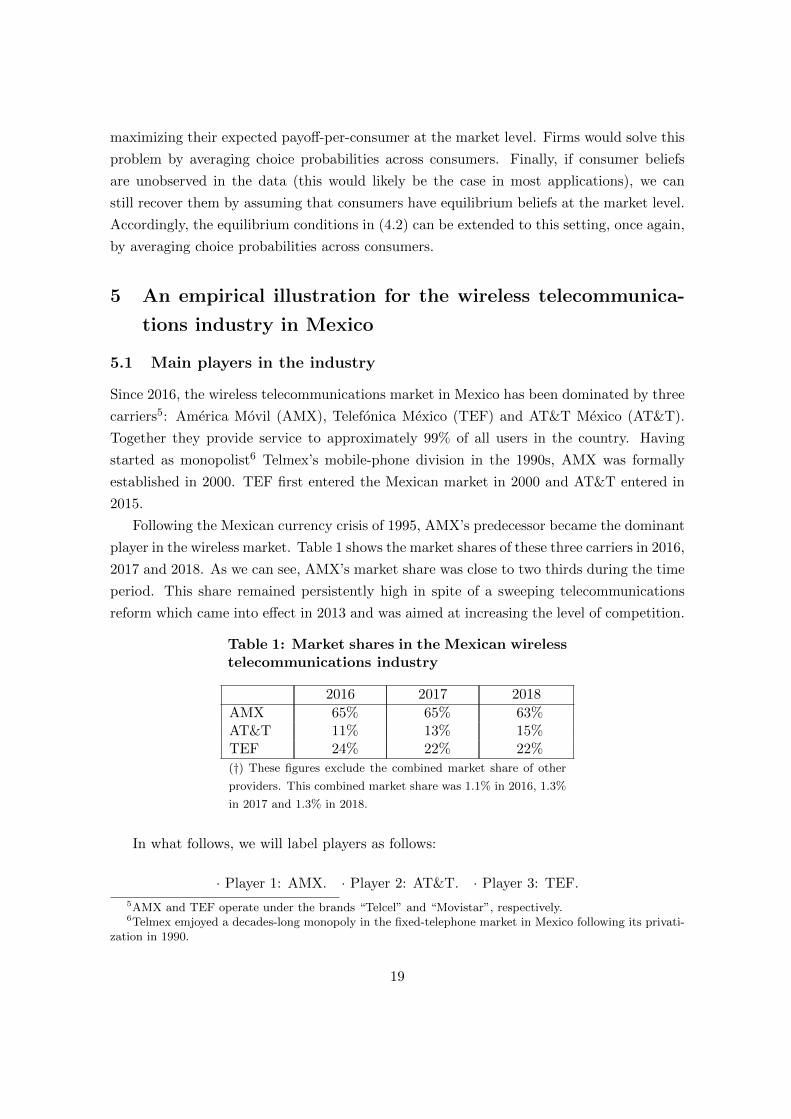
Since 2016, the wireless telecommunications market in Mexico has been dominated by three

carriers5: America Movil (AMX), Telefonica Mexico (TEF) and AT&T Mexico (AT&T).

Together they provide service to approximately 99% of all users in the country. Having

started as monopolist6 Telmex’s mobile-phone division in the 1990s, AMX was formally

established in 2000. TEF first entered the Mexican market in 2000 and AT&T entered in

2015.

Following the Mexican currency crisis of 1995, AMX’s predecessor became the dominant

player in the wireless market. Table 1 shows the market shares of these three carriers in 2016,

2017 and 2018. As we can see, AMX’s market share was close to two thirds during the time

period. This share remained persistently high in spite of a sweeping telecommunications

reform which came into effect in 2013 and was aimed at increasing the level of competition.

Table 1: Market shares in the Mexican wirelesstelecommunications industry

2016 2017 2018

AMX 65% 65% 63%AT&T 11% 13% 15%TEF 24% 22% 22%

(†) These figures exclude the combined market share of other

providers. This combined market share was 1.1% in 2016, 1.3%

in 2017 and 1.3% in 2018.

In what follows, we will label players as follows:

· Player 1: AMX. · Player 2: AT&T. · Player 3: TEF.

5AMX and TEF operate under the brands “Telcel” and “Movistar”, respectively.6Telmex emjoyed a decades-long monopoly in the fixed-telephone market in Mexico following its privati-

zation in 1990.

19

5.2 2013 telecommunications reform in Mexico

Prior to 2013 the telecommunication industry in Mexico was highly concentrated, with AMX

enjoying more than 70% of the market. Lack of competition led to consistently high prices

and a stagnant mobile phone penetration. To address this, the Mexican Congress approved

a sweeping telecommunications reform in 2013 whose main aim was to promote competition

and ensure consumer access to telecommunication services7. The reform established a new

regulator (the Federal Telecommunications Institure or ‘IFT’) with the power to declare

preponderance of the dominant firm (AMX) and impose asymmetrical rules between AMX

and its competitors. Among the most important new regulations, AMX was required to pro-

vide its competitors access to its infrastructure at competitive rates. While the reform led

to the entry of new firms and a decrease in prices, the industry remains highly concentrated

in comparison with other countries and AMX’s market share remains very high by inter-

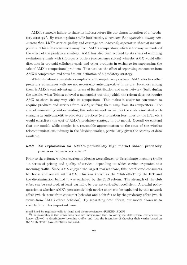
national standards. As Figure 1 and Table 2 illustrate, an international comparison of the

Herfindahl–Hirschman Index8 (HHI) shows that even five years after the reform, the Mexi-

can wireless telecommunications market remained extraordinarily concentrated relative to

other countries in the region, including the United States.

5.2.1 Predatory practices by AMX

Even though the 2013 reform explicitly requires it, AMX has persistently failed to share

its infrastructure (cellphone towers, poles, ducts, conduits, and rights-of-way) in a timely

and effective manner with its competitors. Critics of the reform have pointed out that

the laws enacted lacked the necessary teeth to force AMX to comply. As a result, AMX

has been accused multiple times by its competitors of failing to provide timely access to

its infrastructure9 in a timely and effective way. After several years of this conduct, in

January 2020 the IFT finally took the unprecedented step of imposing a $70-million dollar

fine to AMX for failing to share information about the availability of its telecommunication

7See, for example:• Malkin, Elisabeth (2013-03-11). “Mexican Leaders Propose a Telecom Overhaul”, New YorkTimes. URL: https://www.nytimes.com/2013/03/12/business/global/mexican-plan-would-rein-in-phone-and-tv-providers.html• Estevez, Dolia (2013-05-01). “Mexico’s Congress Passes Monopoly-Busting Tele-com Bill, Threatening Tycoon Carlos Slim’s Business Empire”, Forbes. URL:https://www.forbes.com/sites/doliaestevez/2013/05/01/mexicos-congress-passes-monopoly-busting-telecom-bill-threatening-tycoon-carlos-slims-business-empire/?sh=412beef4b073

8Antitrust authorities in the United States generally classify markets into three types: Unconcentrated(HHI < 1500), Moderately Concentrated (1500 < HHI < 2500), and Highly Concentrated (HHI > 2500).

9Estevez, Dolia (2017-04-10). “Mexico’s Anti-Monopoly Telecom Reform hasDone Little to End Tycoon Carlos Slim’s Market Dominance”, Forbes. URL:https://www.forbes.com/sites/doliaestevez/2017/04/10/mexicos-anti-monopoly-telecom-reform-has-done-little-to-end-tycoon-carlos-slims-market-dominance/?sh=5b137496e9fb

20

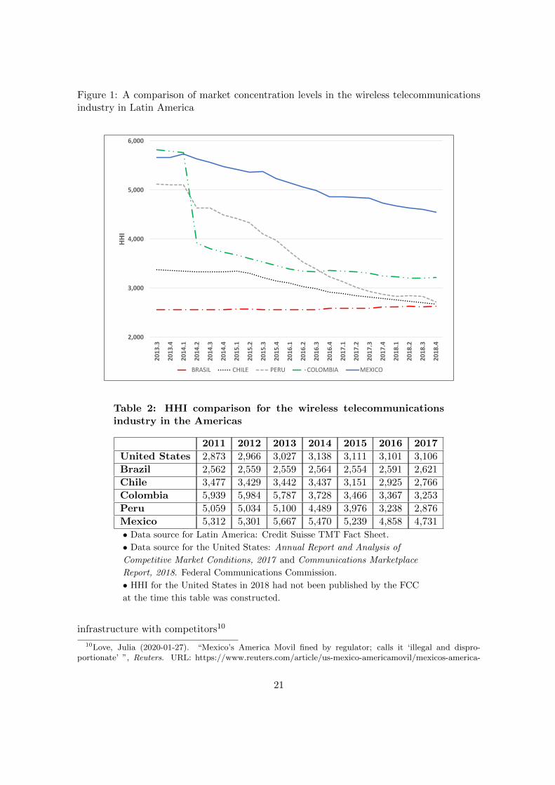
Figure 1: A comparison of market concentration levels in the wireless telecommunicationsindustry in Latin America

2,000

3,000

4,000

5,000

6,000

2013

.3

2013

.4

2014

.1

2014

.2

2014

.3

2014

.4

2015

.1

2015

.2

2015

.3

2015

.4

2016

.1

2016

.2

2016

.3

2016

.4

2017

.1

2017

.2

2017

.3

2017

.4

2018

.1

2018

.2

2018

.3

2018

.4

HHI

BRASIL CHILE PERU COLOMBIA MEXICO

Table 2: HHI comparison for the wireless telecommunicationsindustry in the Americas

2011 2012 2013 2014 2015 2016 2017

United States 2,873 2,966 3,027 3,138 3,111 3,101 3,106

Brazil 2,562 2,559 2,559 2,564 2,554 2,591 2,621

Chile 3,477 3,429 3,442 3,437 3,151 2,925 2,766

Colombia 5,939 5,984 5,787 3,728 3,466 3,367 3,253

Peru 5,059 5,034 5,100 4,489 3,976 3,238 2,876

Mexico 5,312 5,301 5,667 5,470 5,239 4,858 4,731

• Data source for Latin America: Credit Suisse TMT Fact Sheet.

• Data source for the United States: Annual Report and Analysis of

Competitive Market Conditions, 2017 and Communications Marketplace

Report, 2018. Federal Communications Commission.

• HHI for the United States in 2018 had not been published by the FCC

at the time this table was constructed.

infrastructure with competitors10

10Love, Julia (2020-01-27). “Mexico’s America Movil fined by regulator; calls it ‘illegal and dispro-portionate’ ”, Reuters. URL: https://www.reuters.com/article/us-mexico-americamovil/mexicos-america-

21

AMX’s strategic failure to share its infrastructure fits our characterization of a “preda-

tory strategy”. By creating data traffic bottlenecks, it cements the impression among con-

sumers that AMX’s service quality and coverage are inherently superior to those of its com-

petitors. This shifts consumers away from AMX’s competitors, which is the way we modeled

the effect of the predatory strategy. AMX has also been accused by its rivals of enforcing

exclusionary deals with third-party outlets (convenience stores) whereby AMX would offer

discounts in pre-paid cellphone cards and other products in exchange for suppressing the

sale of AMX’s competitors’ products. This also has the effect of separating consumers from

AMX’s competitors and thus fits our definition of a predatory strategy.

While the above constitute examples of anticompetitive practices, AMX also has other

predatory advantages with are not necessarily anticompetitive in nature. Foremost among

them is AMX’s vast advantage in terms of its distribution and sales network (built during

the decades when Telmex enjoyed a monopolist position) which the reform does not require

AMX to share in any way with its competitors. This makes it easier for consumers to

acquire products and services from AMX, shifting them away from its competitors. The

cost of maintaining and expanding this sales network as well as the costs associated with

engaging in anticompetitive predatory practices (e.g, litigation fees, fines by the IFT, etc.)

would constitute the cost of AMX’s predatory strategy in our model. Overall we contend

that our model, while simple, is a reasonable approximation to the state of the wireless

telecommunications industry in the Mexican market, particularly given the scarcity of data

available.

5.2.2 An explanation for AMX’s persistently high market share: predatory

practices or network effect?

Prior to the reform, wireless carriers in Mexico were allowed to discriminate incoming traffic

–in terms of pricing and quality of service– depending on which carrier originated this

incoming traffic. Since AMX enjoyed the largest market share, this incentivized consumers

to choose and remain with AMX. This was known as the “club effect” by the IFT and

the discrimination behind it was outlawed by the 2013 reform. The strength of the club

effect can be captured, at least partially, by our network-effect coefficient. A crucial policy

question is whether AMX’s persistently high market share can be explained by this network

effect (which stems from consumer behavior and habits11) or by the predatory effect (which

stems from AMX’s direct behavior). By separating both effects, our model allows us to

shed light on this important issue.

movil-fined-by-regulator-calls-it-illegal-and-disproportionate-idUSKBN1ZQ2FI11One possibility is that consumers have not internalized that, following the 2013 reform, carriers are no

longer allowed to discriminate incoming traffic, and that the incentives of choosing their carrier based onthe “club effect” have effectively vanished.

22

5.2.3 Data and measures of price and costs

As is the nature of wireless services, each competing firm offers different plans and options12.

Data that could allow us to meaningfully compare prices of equivalent wireless plans between

carriers over time is not publicly available. Furthermore, consumer-level data is also not

available. Our time horizon is also short: AT&T entered the Mexican market in 2015 and

it started to effectively compete in 2016, and final data for 2019 has still not been released

at the time of elaboration of this paper. As a result, we only have comparable data for

the years 2016, 2017 and 2018 and this will be our sample. Lastly, even though quarterly

data is available, variation across quarters within each year is minimal; for this reason, our

empirical illustration will rely on yearly information for 2016, 2017 and 2018. That is, our

data consists of three observations, t = 2016, 2017, 2018, and we will treat each year as an

independent realization of the game described in the previous section. Our methodology

assumes that we observe a measure of prices and costs. These were obtained as follows,

• A price measure. As we mentioned above, there is no publicly available, comparable

data for specific wireless plans13. For this reason we opted to construct an aggregate

price measure for each firm using publicly available information. For each firm ` and

year t we defined

pjt =total wireless service revenue for firm j in year t

total number of active subscribers (active SIM cards) for firm j in year t

Our measure of price is the service revenue per subscriber for each firm. This is

an indicator commonly used in the industry and known as average revenue per user

(ARPU). It aggregates across the different plans offered by each firm but we contend

that variations of this measure across firms and across years should capture the corre-

sponding variation in price levels. By focusing exclusively on mobile service revenue,

our price measure excludes things such as equipment sales and other sources of rev-

enue, thus more credibly capturing only variation in the prices and fees of wireless

plans.

• A measure of the cost of providing service. Using the same logic we construct a

measure of cost-per-consumer of providing service which can be directly comparable

12The Mexican wireless telecommunications market is dominated by prepaid plans. In 2018, approximately83 percent of mobile subscriptions in Mexico were prepaid, whereas 17 percent were postpaid (i.e, paying amonthly rent).

13Also importantly, there is no data available of market shares for specific types of plans, only aggregatemarket shares.

23

to our price measure. For each firm j and year t we defined

cjt =total cost of service for firm j in year t

total number of active subscribers (active SIM cards) for firm j in year t

Table 3 compares the price measures for AT&T and TEF relative to AMX in 2016, 2017

and 2018. As we can see there, these relative prices decreased in all three years. We can

also see that AT&T’s price measure was higher than that of AMX while the opposite was

true for TEF. This reflects the fact that each one of these carriers specializes in different

types of plans. While TEF specializes mostly in cheap, prepaid plans, AT&T is the carrier

with the highest proportion of postpaid plans where customers pay a monthly rent, and

these plans are the most expensive. AMX has a more balanced mix of prepaid and postpaid

plans. Overall, prepaid plans tend to be cheaper and they come with fewer perks and

features. Postpaid plans are more expensive but they have benefits such as more reliable

data speeds. Having firm-specific coefficients in our random utility specifications allows our

model to accommodate this type of product differentiation.

Table 3: A relative comparison of our price measure

2016 2017 2018

(p2t/p1t) 2.08 1.73 1.09(p3t/p1t) 0.64 0.56 0.45

p1t = AMX price measure in year t,

p2t = AT&T price measure in year t,

p3t = TEF price measure in year t.

Table 4 describes our measure of cost of service relative to our measure of price during

the time period analyzed. This proportion remained almost constant for AMX during the

three years analyzed. For AT&T and TEF, it remained approximately constant in 2016

and 2017 and it jumped in 2018. This followed both firms’ aggressive bidding in spectrum

auctions (particularly AT&T) in an effort to expand their 4G capabilities and compete with

AMX. As the table indicates, AT&T had a smaller profit margin than its two competitors

during the period analyzed.

24

Table 4: Cost of service as a proportion of price

2016 2017 2018

(c1t/p1t) 0.38 0.37 0.38(c2t/p2t) 0.69 0.66 0.82(c3t/p3t) 0.37 0.39 0.46

c1t/p1t = AMX in year t,

c2t/p2t = AT&T in year t,

c3t/p3t = TEF in year t.

5.3 An empirical implementation of our model

Parameterization of the utility function

Our representative consumer random utility is parameterized as described in (2.5). That

is,

V1 = −β1 · p1 + λ · πe1 + ξ1, (utility from selecting AMX)

V2 = δ2 − β2 · p2 − γ2 · a+ λ · πe2 + ξ2, (utility from selecting AT&T)

V3 = δ3 − β3 · p3 − γ3 · a+ λ · πe3 + ξ3, (utility from selecting TEF)

Parameterization of the predatory-strategy cost function

We assumed a quadratic cost function for AMX’s predatory strategy. Regarding the cost-

per-consumer for the predatory strategy, we noted first that there was very little change

in the size of the cellphone market Nt during these three years, so we fixed ηt = 1 for the

three periods. Consequently, as discussed in in Section 3.2, we used

artηt

= a2t ,

for the three years observed.

Unknown parameters and observable implications in our empirical example

The model consist of seven parameters,

θ ≡ (δ2, δ3, β1, β2, β3, γ2, γ3) ∈ R7.

25

If we assumed that prices observed are best-response equilibrium prices the model would

produce nine restrictions, as described in (3.6),

p1t = BR1(p2t, p3t, πt|θ, c1t, ηt)

p2t = BR2(p1t, p3t, πt|θ, c2t)

p3t = BR3(p1t, p2t, πt|θ, c3t)

for t = 2016, 2017, 2018.

with ηt = 1 for the three years (for the reasons described above) and quadratic specification

for AMX’s predatory-strategy cost function. Due to the limited nature of our data, we

will take a conservative approach and we will characterize and compute a set of parameter

values θ such that prices observed are “close” to being an equilibrium of the model given

the market shares observed. We describe how we approached this next.

5.3.1 Computing a set of parameter values for which the outcomes observed

in the data are “close” to being an equilibrium of the model

Our limited data set precludes any econometric analysis based on asymptotic theory. How-

ever, the fact that our model produces more restrictions (nine) than the number of param-

eters (seven) means that identifying parameter values that are consistent with our model

(in a well defined sense) and rejecting parameter values that are not, is still a meaningful

exercise and we will undertake it as follows. For a given θ group

BR(pt, πt|θ, ct, ηt) ≡ (BR1(p2t, p3t, πt|θ, c1t, ηt), BR2(p1t, p3t, πt|θ, c2t), BR3(p1t, p2t, πt|θ, c3t))′ .

And let

ρ(pt −BR(pt, πt|θ, ct, ηt);xt) =

1

3

(∣∣p1t −BR1(p2t, p3t, πt|θ, c1t, ηt)∣∣

p1t+

∣∣p2t −BR2(p1t, p3t, πt|θ, c2t)∣∣

p2t+

∣∣p3t −BR3(p1t, p2t, πt|θ, c3t)∣∣

p3t

).

(5.1)

This measures the average percentage difference across the three firms between observed

prices and best-response equilibrium prices predicted by θ in year t. By construction we

have ρ(0;xt) = 0. Let

M(θ) =1

3

2018∑t=2016

ρ(pt −BR(pt, πt|θ, ct, ηt);xt).

26

M(θ) measures the average percentage difference between observed prices and best-response

equilibrium prices for the three firms across the three years observed. Now let

Θ ={θ ∈ Θ: M(θ) < 0.025

}. (5.2)

The set Θ is the collection of parameter values such that the average percentage difference

between observed prices and best-response equilibrium prices is less than 2.5% for our sample.

Computing results based on Θ will be the focus of our empirical exercise. Note that any

θ for which prices observed are exactly an equilibrium of the game would be contained in

Θ. However, by focusing on a set rather than a point (e.g, the global minimizer of M(θ)),

we can compute a range of possible versions of our model that can provide a reasonable

approximation to the outcomes observed in our limited data. From here we can compute

a range of values for the various effects (price, network, predatory strategy) in our model.

Focusing on Θ also helps us avoid having to assume that θ is point-identified or that there

is a unique equilibrium to the game (or that an equilibrium exists at all); we only focus

on finding a set of parameter values for which the observed outcome is “close” to being an

equilibrium of the model, in the sense described in (5.2).

5.3.2 Results

We performed a grid search to find parameter values consistent with criterion (5.2). The

parameter space was constrained as follows,

βj ∈ [0, 6], δj ∈ [0, 6], γj ∈ [0, 6].

Our computation of the best-response prices in (3.6) focused on an interval of ±25% around

the prices observed in the data.

Utility-function parameters

Table 5 presents the range of values for each of the random utility parameters that were

consistent with criterion (5.2). Some of the most interesting findings are the following,

• Even with limited data, our model was able to produce an informative range of pa-

rameter values consistent with criterion (5.2).

• The predatory strategy has a nonzero effect on both of AMX’s competitors, and there

is evidence that this effect is larger for TEF than for AT&T.

• The network effect diminished significantly over time, from 2016 to 2018. This is

consistent with the elimination of the club effect. As we explained above, this was

27

one of the main goals of the 2013 reform.

Table 5: Range of parameter values consistent with criterion (5.2)

Firm-specific coefficientsPredatory-strategy sensitivity

coefficients

δ2 δ3 γ2 γ3

[−0.398,−0.373] [0.810, 0.868] [1.561, 1.646] [2.011, 2.129]

Price-sensitivity coefficients

β1 β2 β3

[2.898, 3.089] [0.825, 0.870] [3.329, 3.565]

Network-effect coefficient λi2016 2017 2018

[0.893, 1.005] [0.110, 0.123] [0.031, 0.049]

The effect of the predatory strategy

Perhaps the easiest way to interpret the magnitude of the predatory-strategy effect is by

looking at the market share elasticities

∂Gjt∂at

atGjt

, for j = 1 (AMX), j = 2 (AT&T) and j = 3 (TEF).

Table 6 presents the results for the range of parameter values consistent with criterion

(5.2). These correspond to the elasticities computed for all the parameter values that were

consistent with said criterion. A summary of the main findings is the following,

• Unlike the network effect, which decreased in magnitude from 2016 to 2018, our results

indicate that the predatory-strategy effect increased during this time period.

• While, in 2016, a 10% increase in at led, approximately14, to an increase of 5.7% (per-

centage change, not percentage points) in AMX’s market share, this figure increased

14This is the mid-point of the interval.

28

to approximately 8.4% in 2018.

• Consistent with our results for (γ2, γ3), the predatory impact of AMX is greater on

TEF than on AT&T.

• In 2016, a 10% increase in at led, approximately, to a decrease of 7.9% and 11.8%

(percentage change, not percentage points) in the market shares of AT&T and TEF,

respectively. In 2018 these figures became 10.9% and 16.6%, respectively.

Table 6: Predatory effect

Predatory effect for AMX: Elasticity of AMX’s market share, G1t with respectto the predatory strategy atatat. Range of values consistent with criterion (5.2).

2016 2017 2018

[0.548, 0.592] [0.724, 0.758] [0.824, 0.860]

Predatory effect for AT&T: Elasticity of AT&T’s market share, G2t with respectto the predatory strategy atatat. Range of values consistent with criterion (5.2).

2016 2017 2018

[−0.811,−0.765] [−1.081,−1.014] [−1.139,−1.054]

Predatory effect for TEF: Elasticity of TEF’s market share, G3t with respect tothe predatory strategy atatat. Range of values consistent with criterion (5.2).

2016 2017 2018

[−1.234,−1.130] [−1.620,−1.515] [−1.704,−1.619]

29

Network effect and the impact of changes in consumers’ beliefs

Our model assumes equilibrium beliefs, but our results can help us study the effect of an out-

of-equilibrium change in the beliefs πet of the representative consumer. Since well-defined

beliefs satisfy πe1t + πe2t + πe3t = 1, it must be the case that if πejt changes exogenously by an

amount ∆πejt, beliefs πe`t and πekt must change by amounts ∆πe`t and ∆πekt respectively, such

that ∆πe1t + ∆πe2t + ∆πe3t = 0. Thus, our exercise must make assumptions about how πe`tand πekt change when πejt changes exogenously. Let us focus on perhaps the most intuitive

scenario and assume the following,

• πejt (the representative consumer’s expected market share of firm j) changes exoge-

nously by an amount ∆πejt such that 0 ≤ πejt + ∆πejt ≤ 1.

• The exogenous change in πejt changes πe`t and πekt (for `, k 6= j) by equal proportional

amounts,

∆πe`t = ∆πekt = −1

2∆πejt,

as long as 0 ≤ πekt + ∆πekt ≤ 1 and 0 ≤ πe`t + ∆πe`t ≤ 1. That is,

∆πejt ≥ 0 =⇒

∆πekt = max{−1

2∆πejt , − πekt}

∆πe`t = max{−1

2∆πejt , − πe`t}

∆πejt ≤ 0 =⇒

∆πekt = min{−1

2∆πejt , 1− πekt}

∆πe`t = min{−1

2∆πejt , 1− πe`t}

Once again, the easiest way to study the impact of a realignment in beliefs is through

market-share elasticities,∂Gmt∂πejt

πejtGmt

.

Table 7 presents the results for the range of parameter values consistent with criterion (5.2).

The main findings can be summarized as follows,

• Consistent with our findings of a decrease in the magnitude of the network effect

λt, market-share elasticities with respect to consumers’ expected market shares also

decreased from 2016 to 2018. This is the outcome the 2013 telecommunications reform

aimed to achieve by eliminating the club effect.

• During the three years analyzed, the market shares of AT&T and TEF were more

sensitive to changes in consumers’ expected market share of AMX than the other way

around. The elasticity of AT&T’s and TEF’s market shares with respect to consumers’

30

expected market share of AMX was about 8 times larger than AMX’s market share

elasticity with respect to changes in consumers’ expected market shares of either

AT&T or TEF. However, the magnitudes of these elasticities decreased steadily.

Table 7: Network effect. Elasticity of Gmt (market share of firmm) with respect to πejt (expected market share of firm j). Range ofvalues consistent with criterion (5.2).

201620162016

G1t G2t G3t

πe1t [0.305, 0.343] [−0.663,−0.566] [−0.663,−0.566]

πe2t [−0.018,−0.016] [0.131, 0.148] [−0.018,−0.016]

πe3t [−0.087,−0.077] [−0.087,−0.077] [0.244, 0.275]

201720172017

G1t G2t G3t

πe1t [0.037, 0.042] [−0.078,−0.070] [−0.078,−0.070]

πe2t [−0.003,−0.002] [0.019, 0.021] [−0.003,−0.002]

πe3t [−0.009,−0.008] [−0.009,−0.008] [0.028, 0.032]

201820182018

G1t G2t G3t

πe1t [0.011, 0.017] [−0.029,−0.019] [−0.029,−0.019]

πe2t [−0.001,−0.001] [0.006, 0.009] [−0.001,−0.001]

πe3t [−0.004,−0.002] [−0.004,−0.002] [0.008, 0.013]

31

Price effects

The final effect we can discuss involves market-share price elasticities,

∂G`t∂pjt

pjtG`t

.

Since each firm has a different mix of pre-paid and post-paid wireless plans and this reflects

in structural differences in price levels across the three firms (as our price measures showed),

a direct comparison of own-price elasticities across the three competitors is a little hard to

interpret. However, an analysis over time of each firm’s own-price elasticity as well as some

discussion about cross-price elasticities is insightful. Table 8 presents the results for the

range of parameter values consistent with criterion (5.2). Some of the main findings are the

following,

• The market share of AMX has become more sensitive to its own price. The elasticity

increased consistently over the three-year period studied. This can be interpreted as a

beneficial effect of the 2013 reform, which has made it easier for consumers to switch

to AMX’s competitors.

• However, the magnitude of the own-price elasticity of AT&T and TEF’s market shares

has decreased over time. This suggests that it has become increasingly difficult for

these firms to attract more consumers through competitive price offers.

• On the other hand, the cross-price elasticity of AT&T and TEF’s market shares

with respect to AMX’s price has increased over time, which suggests that consumers

have switched out of AMX and into its competitors mostly as a response to AMX’s

prices rather than as a reaction to AT&T and TEF’s decreases in prices (which were

continuously observed over the three years studied).

• Consistent with the conjecture that the market has shown a diminished response to

pricing policies of AT&T and TEF, our results suggest that AMX’s market share has

become increasingly less responsive to price changes of its competitors. Overall our

results suggest that it has become increasingly difficult for both of the smaller firms

to directly attract costumers through lower prices.

32

Table 8: Price effect. Elasticity of Gjt (market share of firm j) withrespect to pe`t (price of firm `). Range of values consistent withcriterion (5.2).

201620162016

G1t G2t G3t

p1t [−0.422,−0.395] [0.735, 0.783] [0.735, 0.783]

p2t [0.074, 0.077] [−0.627,−0.594] [0.074, 0.077]

p3t [0.199, 0.214] [0.199, 0.214] [−0.677,−0.633]

201720172017

G1t G2t G3t

p1t [−0.444,−0.415] [0.770, 0.823] [0.770, 0.823]

p2t [0.076, 0.080] [−0.538,−0.509] [0.076, 0.080]

p3t [0.167, 0.180] [0.167, 0.180] [−0.640,−0.598]

201820182018

G1t G2t G3t

p1t [−0.503,−0.471] [0.804, 0.857] [0.804, 0.857]

p2t [0.059, 0.063] [−0.355,−0.337] [0.059, 0.063]

p3t [0.147, 0.156] [0.147, 0.156] [−0.557,−0.519]

33

5.4 Summary of results

• The magnitude of the network effect decreased consistently during the time period

studied. This is consistent with the 2013 reform’s stated goal of eliminating the “club

effect” in the wireless market.

• In contrast, the magnitude of the predatory-strategy effect increased, and our results

consistently suggested that it affected TEF more than AT&T (even though it reduced

both firms’ market shares).

• An ongoing policy discussion in Mexico revolves around whether AMX’s sustained

large market share results from: (a) from consumer habits and a lingering network

effect whereby users have continued to flock to the carrier with the most customers,

or (b) direct predatory actions from AMX. Our results point strongly to the latter, as

the network effect has diminished over time while the impact of the predatory effect

has increased steadily. This points towards the need to supplement the 2013 reform

with more effective oversight of AMX’s practices.

• A study of price elasticities suggests that it has become increasingly difficult for AT&T

and TEF to attract costumers through pricing strategies. In terms of prices, the mar-

ket has responded increasingly more to AMX’s pricing policies rather than those of its

competitors. Our model suggests that AMX has the ability to counteract reductions

in competitors’ prices through predatory practices that shift consumers away.

5.4.1 Divestment of TEF from the Mexican telecommunications market

In November 2019, TEF announced that it would scale back significantly its operations the

Mexican telecommunications market15. They described a gradual process that will take

place in stages, starting with the sale of fibre assets, the migration of mobile subscribers to

AT&T Mexico’s network and the return of spectrum concessions to the regulator (IFT). TEF

will use AT&T’s wireless equipment and will become effectively a mobile virtual network

operator16 (MVNO). The reasons cited by TEF included the predatory practices by AMX

that we enumerated previously, combined with the comparatively expensive cost of the

spectrum in Mexico. The announced effective exit of TEF from the market is in line with

the empirical findings of our model which indicated that AMX’s predatory strategies had a

15Love, Julia (2020-01-27). “Telefonica teams up with AT&T in Mexico in new bid to take fight toSlim ”, Reuters. URL: https://www.reuters.com/article/us-mexico-telefonica/telefonica-teams-up-with-att-in-mexico-in-new-bid-to-take-fight-to-slim-idUSKBN1XV2CM

16An MVNO is a typically smaller wireless carrier that does not own the wireless network infrastructureover which it provides services to its customers.

34

significantly greater impact on TEF than on AT&T and it constitutes an ominous sign for

the future of the industry.

6 Concluding remarks

A number of real-world examples of oligopolistic price competition can be more reason-

ably modeled by assuming that, in addition to prices, a subset of firms have a non-price

“predatory strategy” at their disposal which enables them to shift consumer preferences

away from competitors and towards themselves. This paper proposed an example of such

a model where we treated the predatory strategy as an unobserved market-level random

variable. Ours can be seen as a special case of BLP demand models with the feature that

the unobserved, market-level, product-specific characteristics are modeled explicitly as func-

tions of the unobserved predatory strategy. By presenting a theory of optimal choice for

prices and the predatory strategy, our model allows us to measure the direct effect of the

unobserved predatory strategy. Inspired by our empirical example, our model also included

a “network effect” whereby consumers’ preferences and choices also depend on their sub-

jective expectations of the proportion of other consumers who will choose the product or

service of each firm. We believe this feature can describe a number of interesting real-world

applications.

We applied our model to study the Mexican wireless telecommunications industry, which

has remained heavily concentrated in spite of a 2013 telecommunications reform that was

explicitly aimed at increasing competition. This is an interesting application of our model

since the dominant firm (America Movil or ‘AMX’) has engaged in documented (and re-

cently sanctioned) practices that fit our model’s description of predatory strategies. One

of our main questions was whether the persistently high market share of AMX was the re-

sult of the network effect (whereby consumers are driven to select the largest carrier) or the

predatory-strategy effect (by which AMX’s predatory practices directly shift consumer pref-

erences away from its competitors). Using data from 2016-2018, our results indicated that

the network effect diminished steadily over time while the predatory effect increased. The

recent exit of one of AMX’s two main competitors from the Mexican market is a worrisome

outcome that is in line with our empirical results.

35

References

Andrews, D. W. K. and X. Shi (2013). Inference for parameters defined by conditional

moment inequalities. Econometrica 81 (2), 609–666.

Berry, S., P. Haile, and A. Gandhi (2013). Connected substitutes and invertibility of

demand. Econometrica 81, 2087–2111.

Berry, S., J. Levinsohn, and A. Pakes (1995). Automobile prices in market equilibrium.

Econometrica 63, 841–890.

Chen, Y., A. Roayaei, and B. Seldon (1993). Cooperative and predatory advertising:

Effects on oligopoly advertising investment. Atlantic Economic Journal 21, 26–38.

de la Fuente, A. (2000). Mathematical methods and models for economists. Cambridge

University Press.

Dominguez, M. and I. Lobato (2004). Consistent estimation of models defined by condi-

tional moment restrictions. Econometrica 72 (5), 1601–1615.

Gale, D. and H. Nikaido (1965). The jacobian matrix and the global univalence of map-

pings. Mathematische Annalen 159, 81–93.

Gundlach, G. (1990). Predatory practives in competitive interaction: Legal limits and

antitrust considerations. Journal of Public Policy & Marketing 9, 129–153.

McFadden, D. (1974). Conditional logit analysis of qualitative choice behavior. In

P. Zarembka (Ed.), Frontiers of Econometrics, pp. 105–142. New York: Academic.

Nevo, A. (2000). A practitioner’s guide to estimation of random-coefficients logit models

of demand. Journal of Economics & Management Strategy 9 (4), 513–548.

Nevo, A. (2011). Empirical models of consumer behavior. Annual Review of Economics 3,

51–75.

Newey, W. and D. McFadden (1994). Large sample estimation and hypothesis testing.

In R. Engle and D. McFadden (Eds.), The Handbook of Econometrics, Volume 4, pp.

2111–2245. North-Holland.

36

Documents

An Empirical Model of Price Competition with Predatory