AN EMPIRICAL ANALYSIS OF PETROLEUM PRODUCTS DEMAND … · AN EMPIRICAL ANALYSIS OF PETROLEUM PRODUCTS DEMAND IN ... this study applied the approach ... in the estimation of the models

Global Journal of Arts Humanities and Social Sciences

Vol.2, No.4, pp.53-71, June 2014

Published by European Centre for Research Training and Development UK (www.ea-journals.org)

53

AN EMPIRICAL ANALYSIS OF PETROLEUM PRODUCTS DEMAND IN

NIGERIA: A RANDOM TREND APPROACH

Mathew Adagunodo

Department Of Economics, C0llege of Management and Social Sciences

Osun State University, Okuku Campus, Osogbo

ABSTRACT: The main objective of this study is to estimate petroleum products demand using a

random trend approach with aim of deriving improved and more robust estimates of price and

income elasticities. The study specifies the random trend model of petroleum products demand as

a two-step stochastic process. The estimates of model parameters for each petroleum products, in

Nigeria are obtained by applying maximum likelihood in conjunction with Kalman filter. The study

revealed that the introduction of random trend reduces the estimate of the coefficient of the lagged

dependent variable in the three petroleum products relative to no trend model. As a result, price

and income elasticities of petroleum product demands are higher in the short run and long run

relative to constant intercept model. The introduction of random trend leads to improvement in

the mean square errors of within sample forecasts.

KEYWORDS: Elasticity, Kalman Filter, Maximum Likelihood and Energy Demand.

JEL: D12, Q4 AND Q41

INTRODUCTION

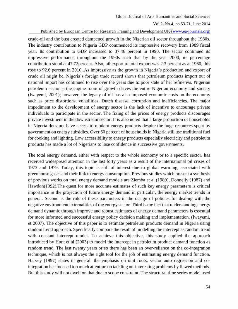
The Nigeria’s economic policies and growth have been influenced by energy sector for more than

four decades particularly the oil sector. Since the global energy crisis of 1972/73, the energy sector,

particularly the petroleum subsector of the Nigerian economy has become the most important

source of revenue, particularly foreign exchange earnings. Although, crude oil production and

export commenced in Nigeria in 1958, the oil sector of the economy did not achieve its present

pre-eminent position until the mid-1970s, a rise aided by rising national production level and the

hike in international price resulting from 1973 Arab-Israel war. The period of 1970 to 1980

represent Nigeria’s oil boom era in term of production, export and earnings from exports. Peak

production in the boom era was achieved in 1979 with a yearly production of 845.463 billion barrel

representing an average daily production of 2.3bpd (CBN, 2008).In view of the strategic nature of

the petroleum industry as the predominant source of global energy, it has become a prime source

of revenue generation to many countries, particularly in Nigeria. The oil sector contribution to

Gross Domestic Product (GDP) at current basic prices was as low as 0.9 percent of GDP in 1961.

With increase in exploration and production related activities consequent on the boom of the 1970s

the sector contribution to GDP has risen to 28.48 percent by 1980.The slump in world price of

http://www.ea-journals.org/


Vol.2, No.4, pp.53-71, June 2014


54

crude-oil and the bust created dampened growth in the Nigerian oil sector throughout the 1980s.

The industry contribution to Nigeria GDP commenced its impressive recovery from 1989 fiscal

year. Its contribution to GDP increased to 37.46 percent in 1990. The sector continued its

impressive performance throughout the 1990s such that by the year 2000, its percentage

contribution stood at 47.72percent. Also, oil export to total export was 2.3 percent as at 1960, this

rose to 92.6 percent in 2010 .As impressive as the growth in Nigeria’s production and export of

crude oil might be, Nigeria’s foreign trade record shows that petroleum products import out of

national import has continued to rise over the years due to poor state of her refineries. Nigerian

petroleum sector is the engine room of growth drives the entire Nigerian economy and society

(Iwayemi, 2001); however, the legacy of oil has also imposed economic costs on the economy

such as price distortions, volatilities, Dutch disease, corruption and inefficiencies. The major

impediment to the development of energy sector is the lack of incentive to encourage private

individuals to participate in the sector. The fixing of the prices of energy products discourages

private investment in the downstream sector. It is also noted that a large proportion of households

in Nigeria does not have access to modern energy products despite the huge resources spent by

government on energy subsidies. Over 60 percent of households in Nigeria still use traditional fuel

for cooking and lighting. Low accessibility to energy products especially electricity and petroleum

products has made a lot of Nigerians to lose confidence in successive governments.

The total energy demand, either with respect to the whole economy or to a specific sector, has

received widespread attention in the last forty years as a result of the international oil crises of

1973 and 1979. Today, this topic is still of interest due to global warming, associated with

greenhouse gases and their link to energy consumption. Previous studies which present a synthesis

of previous works on total energy demand models are Ziemba et al (1980), Donnelly (1987) and

Hawdon(1992).The quest for more accurate estimates of such key energy parameters is critical

importance in the projection of future energy demand in particular, the energy market trends in

general. Second is the role of these parameters in the design of policies for dealing with the

negative environment externalities of the energy sector. Third is the fact that understanding energy

demand dynamic through improve and robust estimates of energy demand parameters is essential

for more informed and successful energy policy decision making and implementation. (Iwayemi,

et 2007). The objective of this paper is to estimate petroleum products demand in Nigeria using

random trend approach. Specifically compare the result of modelling the intercept as random trend

with constant intercept model. To achieve this objective, this study applied the approach

introduced by Hunt et al (2003) to model the intercept in petroleum product demand function as

random trend. The last twenty years or so there has been an over-reliance on the co-integration

technique, which is not always the right tool for the job of estimating energy demand function.

Harvey (1997) states in general, the emphasis on unit roots, vector auto regression and co-

integration has focused too much attention on tackling un-interesting problems by flawed methods.

But this study will not dwell on that due to scope constraint. The structural time series model used



Vol.2, No.4, pp.53-71, June 2014


55

to represent the random shift in demand relies only on a few parameters and yet it is quite general

in the sense that it rests several well known models such as random walks, fixed trends or trends

at all (Andrews 1999; Khalaf and Kichian, 2005).

The random trend model adopted to estimate price and income elasticity for petroleum products

using aggregates and disaggregates approach using annual data covers 1980-2010. The specific

products that considered are automotive gas oil (Diesel), premium motor spirit (petrol) and dual

purpose kerosene (household kerosene) measured in tonnes per capita. The rest of this paper is

organised into four sections. Following this introduction is section two. It features conceptual,

theoretical and empirical issues. The research methodology is discussed in section three;

Empirical result and analysis of regression results are contained in section four. Summary and

some concluding remarks are including in section five.

CONCEPTUAL, THEORETICAL AND EMPIRICAL ISSUES

Since most macro variables are highly trended, deterministic trends are used in unit root tests and

in the estimation of the models with cointegration techniques. The implication of allowing for

deterministic trend is that if the model is shocked, after some departures from the trend, the

variables would return to their trend values. Cointegration techniques ensure this by estimating the

model so that the residuals are stationary. Therefore, shocks have no permanent effects on the trend

in the equilibrium relationships. Ventosa-Santaularia and Gomez (2007) proved that it is incorrect

to carry out standard hypothesis testing on the deterministic trend parameter estimated with

Dickey-Fuller (DF)-type tests when there is a unit root since the limiting distribution of its t-

statistic is neither asymptotically normal with unit variance nor nuisance-parameter-free when the

innovations are not independent and normal distribution.The Cointegration approach can only

accommodate a deterministic trend and deterministic seasonal dummies. In contrast Harvey (1997)

argued that unless the time period is fairly short, these trends cannot be adequately captured by

straight lines. In other words, a deterministic linear time trend is too restricting. Harvey suggests

that time series models should incorporate slowly evolving stochastic instead of deterministic

trends. Such models are known as the unobserved components models or structural time series

models. Models with stochastic trends i.e., structural time series models are useful in some

instances. Firstly, it may be hard to identify multiple structural breaks in the deterministic trend

when the sample size is small. Secondly, in structural time series models, standard classical

methods of estimation can be used to estimate the effects of additional explanatory variables (Rao

2007)

In standard economic models, individual decision-making is based on the assumptions of rational

behaviour and self-interest, according to which individuals make choices that maximize their well-

being or utility under the constraints they face. These assumptions are often supported by empirical

evidence: people facing policy incentives will respond generally in a manner consistent with



Vol.2, No.4, pp.53-71, June 2014


56

welfare maximisation. The main economic factors driving energy demand in households are prices

and income. It is also known from basic economic theory that there is a close link between price

elasticity and substitution possibilities. A household facing higher energy prices can typically use

a whole array of different ways to lessen the impact of the price increase on their budget. Because

these substitution possibilities vary across households the price elasticity’s varies across the

population. Therefore demand for energy is generally quite price-inelastic. Income is a key driver

of energy demand, if the relative price of energy increases, the reductions of demand are expected

(Huntington, H. 1987). Pricing will induce a change in consumption decisions. It is widely

accepted among analysts that the quantity demanded of a good or service has an inverse

relationship with the price. This general perception derives as much from common sense as from

economic theory and basic data observation. Given the significance of this phenomenon,

economists have developed a specific concept called price elasticity which measures the relative

change (%) in quantity demanded for a good or a service, in response to a relative change (%) in

price. Price elasticities can be useful for studying the expected demand growth of a good or service,

and for analysing the impact of different government actions with respect to prices such as tariffs,

taxes or consumption-related subsidies. The positive link between the consumption of a good or

service and the income is also widely acknowledged. That is the relative change (%) in quantity

demanded which results from a relative change (%) in the income.

Petroleum products demands like any other commodities are a multivariable relationship, that is

it is determined by many factors simultaneously. The traditional theory of demand has

concentrated on four of the determinants the price of petroleum products, price of other energy,

income of the consumers and habit. The traditional theory of demand examines only the final

consumers demand for durable and non durables. It is partial in its approach in that it does not

examine the demand in other markets. The serious difficulties that associate with such estimating

function are the aggregation of demand over individual and over commodities makes the use of

index numbers inevitable. Furthermore, there are various other estimation problems which impair

the reliability of the statistically estimated demand functions. The most important of these

difficulties arise from simultaneous change of all determinants, which makes it extremely difficult

to assess the influence of each individual factor separately. However, there has been a continuous

improvement in the economic technique.There is a considerable economic literature on energy

demand. Although the first empirical papers can be traced back to the 1950s, the energy crises of

the 1970s led to a subsequent larger interest .One of the most comprehensive surveys of energy

demand modelling was prepared by Douglas R. Bohi (1981) for the Electric Power Research

Institute. (EPRI). The overall purpose of the study was to examine price elasticities, the study is

an excellent overview of demand modelling since price elasticities are usually output derived from

an overall analysis of demand determinants. An update of this study was prepared in 1984 by Bohi

and Zimmerman. Madlener (1996) attempts to update the earlier Bohi work, as well as breaking

the existing econometric literature into a number of useful different categories. These include

studies associated with log-linear functional forms, transcendental logarithmic (translog)

functional forms, qualitative choice models (also known as discrete choice models), household

prod uction theory (end-use modelling) and pooled time series – cross sectional models. A first



Vol.2, No.4, pp.53-71, June 2014


57

general approach consists of estimating the energy using aggregate demand analysis model on

prices and income (GDP) and climate conditions (Narayan and Symth 2005; Hondroyians 2004).

The second group uses micro economic data to estimate the demand for energy goods (Hanemann

1984; Bernard 1996; Baker 1995 and Vaage 2000). Allowing some additional explanatory

variables as the stock of durable goods (heating systems stock of electric appliances, etc) housing

(size, age of house, insulation etc) and household characteristic (number of members age, income

etc).Though literature has a long standing on energy demand; there is still a paucity of research on

energy demand in Africa and Nigeria in particular. Previous studies have concentrated on

aggregate approach. Also the fact that some of these studies have been done long ago makes a new

study in this area very imperative. In addition the review studies focus on cointegration

approaches.

Iwayemi et al (2007) using multi variable cointegration approach for 1977 to 2006 annual data

confirm the conventional wisdom that energy consumption responds positively to changes in GDP

and negative respond to change in energy price. Gasoline has the highest long run income elasticity

followed by total energy demand. The lowest long run income elasticity has recorded by diesel in

absolute terms. In similar run, kerosene has the highest long run price elasticity followed by diesel

in absolute term. Onwioduokit and Adenuga (1998) employed cointegration techniques to estimate

elasticities for proportions of GDP contributed by agriculture, manufacturing and services. Their

empirical findings reveal that urbanization was one of the principal factors that have a positive

impact on the consumption of liquefied petroleum gas and premium motor spirit. De vita et al.,

(2006) using database of end-user local energy data and Auto Regressive Distributive Lag (ARDL)

bound testing approach to cointegration to estimate the long-run elasticities of Namibian energy

demand function at both aggregate level and by type of energy (electricity, petrol and diesel) for

the period 1980 to 2002, their result shows that energy consumption respond positively to GDP

and negatively to price and temperature. However, previous studies in Nigeria do not model

intercept as random trend. As a consequence, the price effects obtained may not be accurate and

may lead to a wrong assessment on the effectiveness and costs of energy policies.Thus create an

important gap to be filled in this study.

RESEARCH METHODOLOGY

The Structural Time Series Model (STSM) is adopted in this study, since it is consistent with

interpretation of the underlying Energy Demand Trend (UEDT). In particular, it allows for time

estimation of a non-linear UEDT that can be negative, positive or zero over the estimation period.

The Model

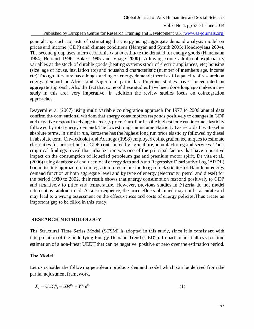
Let us consider the following petroleum products demand model which can be derived from the

partial adjustment framework.

teYXPXUXa

t

a

t

a

ttt

321

1 (1)



Vol.2, No.4, pp.53-71, June 2014


58

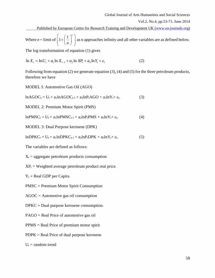
Where e = limit of as n approaches infinity and all other variables are as defined below.

The log transformation of equation (1) gives

tttttt YaXPaXaUX lnlnlnlnln 3211 (2)

Following from equation (2) we generate equation (3), (4) and (5) for the three petroleum products,

therefore we have

MODEL I: Automotive Gas Oil (AGO)

lnAGOCt = Ut + a1lnAGOCt-1 + a2lnPtAGO + a3lnYt+ t. (3)

MODEL 2: Premium Motor Spirit (PMS)

lnPMSCt = Ut + a1lnPMSCt-1 + a2lnPtPMS + a3lnYt+ t. (4)

MODEL 3: Dual Purpose kerosene (DPK)

lnDPKCt = Ut + a1lnDPKCt-1 + a2lnPtDPK + a3lnYt+ t. (5)

The variables are defined as follows:

Xt = aggregate petroleum products consumption

XPt = Weighted average petroleum product real price.

Yt = Real GDP per Capita

PMSC = Premium Motor Spirit Consumption

AGOC = Automotive gas oil consumption

DPKC = Dual purpose kerosene consumption.

PAGO = Real Price of automotive gas oil

PPMS = Real Price of premium motor spirit

PDPK = Real Price of dual purpose kerosene

Ut = random trend

11

n

n



Vol.2, No.4, pp.53-71, June 2014


59

𝜖t.= random error term

a1, a2, a3 are structural parameters of interest.

The random error term t is assumed to be normally and independently distributed (NID) with

mean 0 and variance 2.

Following Hunt et al. (2003) the random trend is assumed to evolve according to the following

stochastic process:

and nt ~ NID (0, 2n.) (6)

ttt 1 and t ~ NID (0, 2.) (7)

Equation (6) represents the level of the trend and equation (7) represents its stochastic slope. This

is a general and yet parsimonious parametric specification of an evolving random trend. Several

well known cases are subsumed under equation (6) and (7) according to the values that are taken

by .

If 0δ and 0 0,β 2

n

2

ε0 we have random walk. If β0 ≠ 0, 2=0 and 2

≠0, we get constant

trend. Once the influence of fundamental variables such as energy price, income and other

explanatory variables have been taken into account, which is known about how energy intensity is

evolving over time as a result of technological change in particular. The model specified here is

quite flexible and impose no constraint on the speed and the level of adjustment as we encounter

in models with a constant trend as no trend at all.

The log linear model with lag dependent variables with or without a constant trend has been used

extensively to model petroleum product demand. The introduction of the lag structure is an ad hoc

way of taking into account the fact that stock of energy using equipments is adjusting slowly

overtime in response to various factors including energy prices (Walkers and Wirl, 1993; Arsenault

et al., 1995;Gately and Huntington,2002; Griffin and Schulman 2005).

The solution to equation (7), for example is

t

i

t

1

01

Where o is initial value of this parameter.

1 1t t t tU U n

2 2

0 0, , and n



Vol.2, No.4, pp.53-71, June 2014


60

The important point to note is that random shocks have a permanent effect on slope parameter. A

similar interpretation can be given to equation (6) where random shocks have permanent effects

on the level of trend. Note that both parameters evolve over time and capture the cumulative effects

of the two random shocks n and . If the variances of these error terms one zero i.e. n2 = 0 and

2 = 0, they are no more stochastic shock and the trend becomes deterministic. The equation to

be estimated therefore consist of equation (3) with (4) (5) (6) and (7). All the disturbance term are

assumed to be independent and mutually uncorrelated with each other. The hyper parameters have

an important role to play and govern the basic properties of the model. The hyper parameters,

along with the model are estimated by maximum likelihood and from these the optimal estimates

of t and Ut are estimated by the Kalman filters which represent the latest estimates of the level

and slope of the trend.

The optimal estimates of the trend over the whole sample period are further calculated by the

smoothing algorithm of the Kalman filters. For model evaluation, equation residuals are estimated

(which are estimates of the equation disturbance term, similar to those from ordinary regression)

plus a set of auxiliary residuals include smoothened estimates of the equation disturbances (known

as the level residuals) and smoothened estimates of the slope disturbance (known as the slope

residuals). Further, to avert the problem of ‘spurious regression’, the time series characteristics of

the variables using the Dickey-Fuller (DF), Augmented Dickey-Fuller (ADF) and Phillips-Perron

(P-P) tests were first examined. Basically, the idea is to ascertain the order of integration of the

variables as to whether they are stationary I(0) or non-stationary; and, therefore, the number of

times each variable has to be differenced to arrive at stationarity.

The standard DF test is carried out by estimating the following;

tttt xyy

'

1 ……………………………………………………………(8)

After subtracting 1ty from both sides of the equation:

tttt xyy

'

1 ………………………………………………………..…(9)

Where = 1

The null and alternative hypotheses may be written as:

H0 : = 0

H1 : < 0



Vol.2, No.4, pp.53-71, June 2014


61

The simple Dickey-Fuller unit root test described above is valid only if the series is an AR(1)

process. If the series is correlated at higher order lags, the assumption of white noise disturbances

t is violated. The Augmented Dickey-Fuller (ADF) test constructs a parametric correction for

higher-order correlation by assuming that the y series follows an AR(P) process and adding P

lagged difference terms of the dependent variable y to the right-hand side of the test regression:

tptpttttt vyyyxyy ...2211

'

1 ………………………(10)

The usual practice is to include a number of lags sufficient to remove serial correlation in the

residuals and for this; the Akaike Information Criterion is employed.

Phillips and Perron (1988) propose a non-parametric alternative method of controlling for serial

correlation when testing for a unit root. The P-P method estimates the non-augmented DF test

equation (9), and modifies the t-ratio of the coefficient so that serial correlation does not affect

the asymptotic distribution of the test statistic. The PP test is based on the statistic:

sf

sefT

ftt

2

1

2

1

0

00

0

0

2

ˆ)(

…………………………………………(11)

Where ̂ is the estimate, and t the t-ratio of , ̂se is the coefficient standard error, and s is

the standard error of the test regression. In addition, 0 is a consistent estimate of the error variance

in equation (9) (calculated as (T – K)s2 where k is the number of regressors). The remaining term,

f0, is an estimator of the residual spectrum at frequency zero.

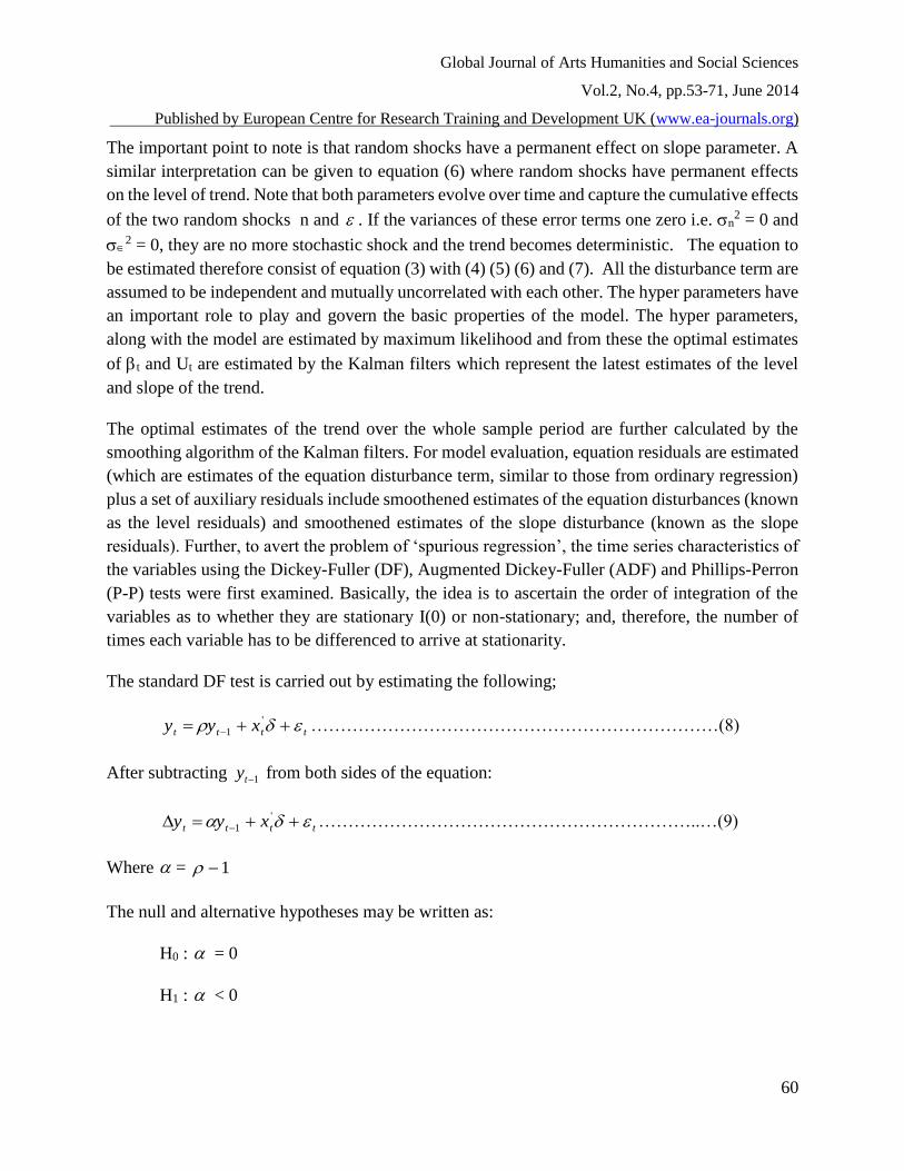
EMPIRICAL RESULTS

Table 1: Descriptive Statistics of Petroleum Products

STATISTICS CAGO CDPK CPMS PAGO PDFK PPMS

Mean 1018627.22 1422992.50 4228338.20 1060.39 949.77 1100.78

Minimum 256158 686719 1861618 0.11 0.15 0.153

Maximum 2368115 2161368 8644263 7800 6950 6500

Std. Dev 694380.59 379318.01 1610653.82 1774.87 1635.48 1635.33

Observation 30 30 30 30 30 30

Source: Author computation



Vol.2, No.4, pp.53-71, June 2014


62

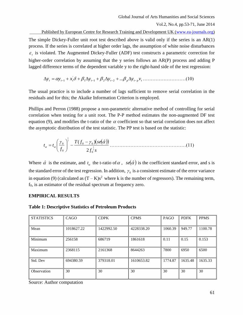
Table 1 above shows the consumption of AGO as ranging from the lowest value of 256,158 metric

tonnes to 2,368,115 metric tonnes with a mean value of 1,018,627.22 metric tonnes. DPK exhibits

a mean value of 1,422,992.5 metric tonnes, while the mean consumption of PMS, for the sample

period is 4,228,338.20 metric tonnes. .

Figure 1: Trends of per capita Premium Motor Spirit Consumption

Source: Author computation using E-view 7

PMS Price(k)

3400200070400

Pe

r C

ap

ita

Co

nsu

mp

tio

n P

MS

80000

70000

60000

50000

40000

30000

20000



Vol.2, No.4, pp.53-71, June 2014


63

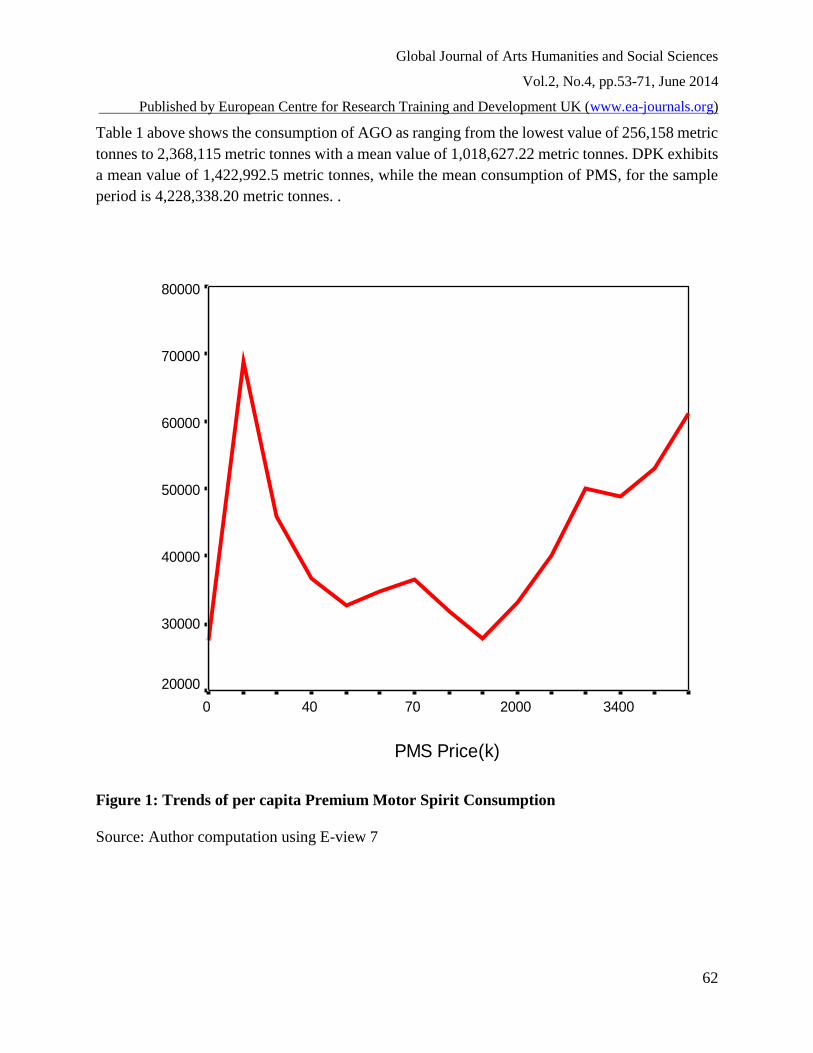
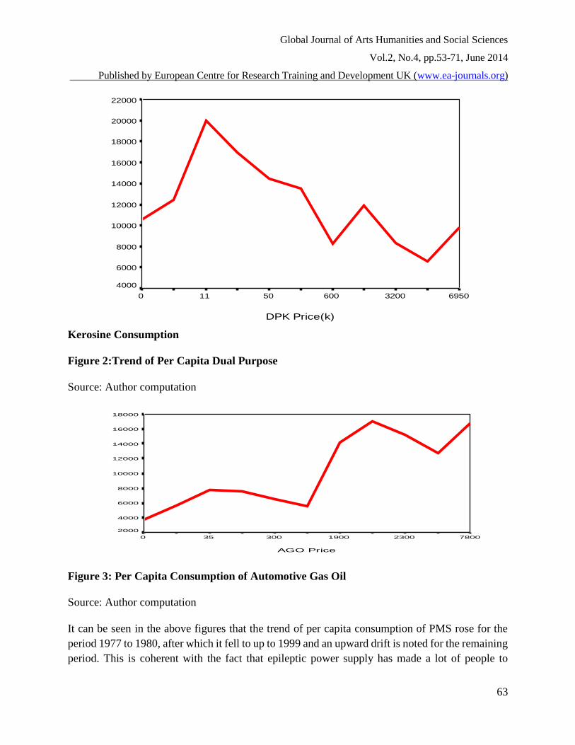
Kerosine Consumption

Figure 2:Trend of Per Capita Dual Purpose


Figure 3: Per Capita Consumption of Automotive Gas Oil


It can be seen in the above figures that the trend of per capita consumption of PMS rose for the

period 1977 to 1980, after which it fell to up to 1999 and an upward drift is noted for the remaining

period. This is coherent with the fact that epileptic power supply has made a lot of people to

DPK Price(k)

6950320060050110

Per

Cap

ita C

onsu

mpt

ion

DP

K

22000

20000

18000

16000

14000

12000

10000

8000

6000

4000

AGO Price

780023001900300350

Per C

apita

Cons

umpti

on AG

O(k)

18000

16000

14000

12000

10000

8000

6000

4000

2000



Vol.2, No.4, pp.53-71, June 2014


64

purchase power generating plant that is using petrol engine since cost of diesel is high. It can also

be as a result of rising income which led to massive importation of fairly used vehicles with high

consumption of fuel. Overall, the per capita consumption of dual purpose kerosene (DPK) is

decreasing over the sample period. This decrease in consumption could be as a result of

substituting household gas (LPO) for kerosene due to increase in income of the consumers. It can

also be linked to the fact that a lot of low income earners that cannot afford the high cost of

kerosene have changed to traditional fuels like charcoal, fuel wood and sawdust. Finally, improved

industrialisation activities have led to increased per capita consumption of automatic gas oil due

to incessant power supply.

Stationarity Test

The time series behaviour of each of the series is presented in Table 2 below, using the ADF and

P – P tests.

Table 2: Unit Root Tests

Variable ADF P – P Decision

DLnPCRGDP -2.0260 -2.2308 I (1)

DlnPCAGO -1.7645 -1.5963 I (1)

DLnPCDPK -2.1078 -2.1427 I (1)

DLnPCPMS -2.3600 -2.5035 I (1)

DLnRPAGO -2.1705 -1.8217 I (1)

DLnRPDPK -1.5712 -1.8217 I (1)

DLnRPPMS -2.3983 -1.9947 I (1)

Critical values

1% = -3.6892

5% = 2.9719

Critical values

1% = -3.6892

5% = 2.9719


The results presented in table 2 above depicts that all the variables are homogenous of order one.

Therefore, they are made stationary by first difference prior to subsequent estimations to forestall

spurious regressions.

Random Trend Model

Table 3 shows the estimation results; for the sake of comparison we also present in table 4 the

estimation results for the model with constant intercept. Although the no trend model is nested

within the more general stochastic trend. We cannot apply the standard log-likelihood ratio test

procedure to determine whether there is a statistically significant difference between the random

trend and no trend model. The random trend model collapses to the no trend model at the boundary



Vol.2, No.4, pp.53-71, June 2014


65

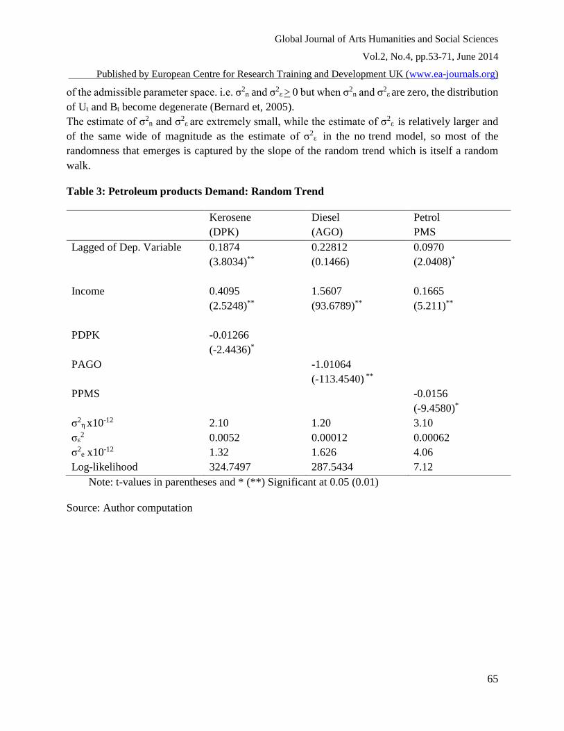
of the admissible parameter space. i.e. σ2n and σ2

ε > 0 but when σ2n and σ2

ε are zero, the distribution

of Ut and Bt become degenerate (Bernard et, 2005).

The estimate of σ2n and σ2

ε are extremely small, while the estimate of σ2ε is relatively larger and

of the same wide of magnitude as the estimate of σ2ε in the no trend model, so most of the

randomness that emerges is captured by the slope of the random trend which is itself a random

walk.

Table 3: Petroleum products Demand: Random Trend

Kerosene

(DPK)

Diesel

(AGO)

Petrol

PMS

Lagged of Dep. Variable 0.1874

(3.8034)**

0.22812

(0.1466)

0.0970

(2.0408)*

Income 0.4095

(2.5248)**

1.5607

(93.6789)**

0.1665

(5.211)**

PDPK -0.01266

(-2.4436)*

PAGO -1.01064

(-113.4540) **

PPMS -0.0156

(-9.4580)*

σ2η x10-12 2.10 1.20 3.10

σε2 0.0052 0.00012 0.00062

σ2e x10-12 1.32 1.626 4.06

Log-likelihood 324.7497 287.5434 7.12

Note: t-values in parentheses and * (**) Significant at 0.05 (0.01)




Vol.2, No.4, pp.53-71, June 2014


66

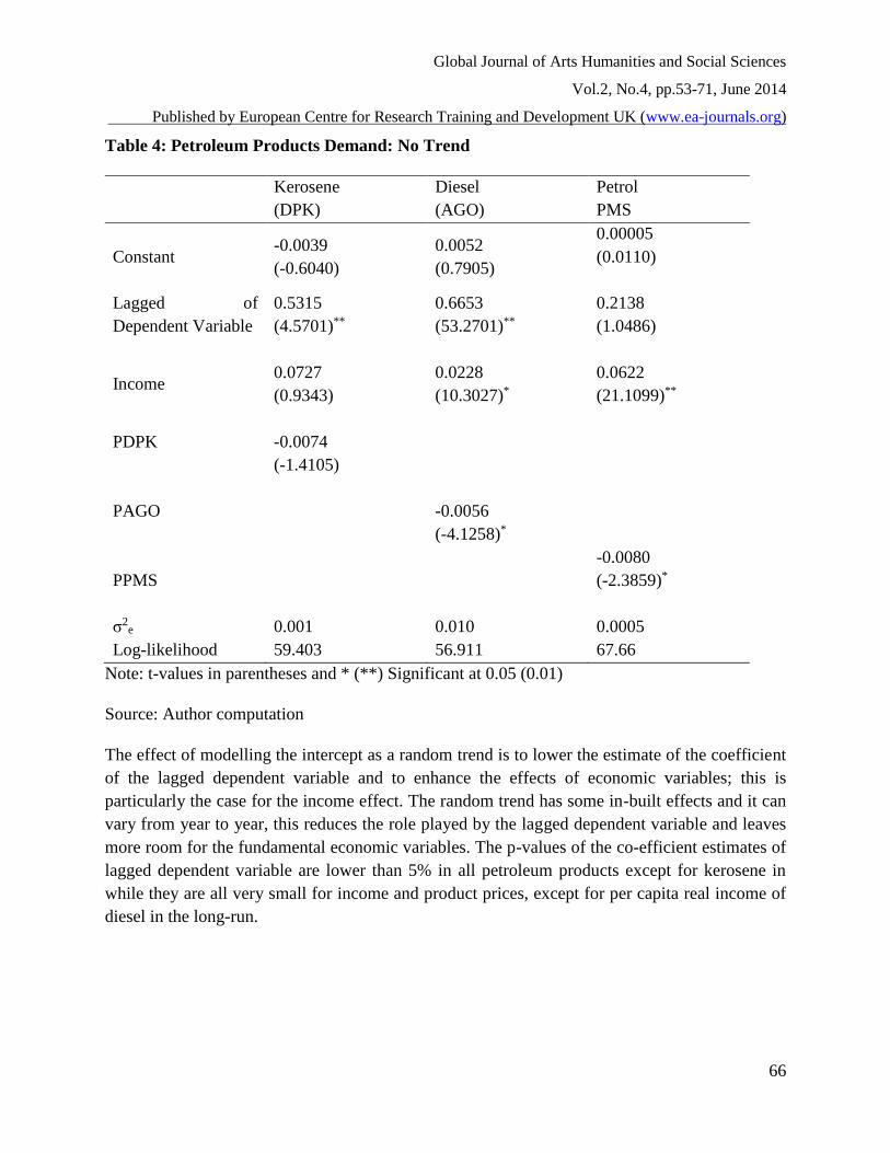
Table 4: Petroleum Products Demand: No Trend

Kerosene

(DPK)

Diesel

(AGO)

Petrol

PMS

Constant -0.0039

(-0.6040)

0.0052

(0.7905)

0.00005

(0.0110)

Lagged of

Dependent Variable

0.5315

(4.5701)**

0.6653

(53.2701)**

0.2138

(1.0486)

Income 0.0727

(0.9343)

0.0228

(10.3027)*

0.0622

(21.1099)**

PDPK

-0.0074

(-1.4105)

PAGO

-0.0056

(-4.1258)*

PPMS

-0.0080

(-2.3859)*

σ2e 0.001 0.010 0.0005

Log-likelihood 59.403 56.911 67.66

Note: t-values in parentheses and * (**) Significant at 0.05 (0.01)


The effect of modelling the intercept as a random trend is to lower the estimate of the coefficient

of the lagged dependent variable and to enhance the effects of economic variables; this is

particularly the case for the income effect. The random trend has some in-built effects and it can

vary from year to year, this reduces the role played by the lagged dependent variable and leaves

more room for the fundamental economic variables. The p-values of the co-efficient estimates of

lagged dependent variable are lower than 5% in all petroleum products except for kerosene in

while they are all very small for income and product prices, except for per capita real income of

diesel in the long-run.



Vol.2, No.4, pp.53-71, June 2014


67

The Short Run and Long Run Elasticity of the Estimates for The Random and No Trend

Table 5 shows the short run and long run price and income elasticities estimates for the random

trend and the no trend models.

Table 5:Demand Elasticities

DIESEL (AGO) KEROSENE (DPK) PETROL (PMS)

S.R L.R S.R L.R S.R L.R

RANDOM TREND

PRICE -0.0106 -0.1270 -0.0127 -0.0132 -0.0106 -0.0126

INCOME 1.5607 2.0138 0.4095 4.0180 0.1665 0.5133

NO TREND

PRICE -0.0056 -0.0077 -0.0074 -0.0112 -0.0080 -0.0110

INCOME 0.00228 0.0057 0.0727 0.1702 0.0622 0.2360

Source: Own estimation

According to commonly used statistical criteria, the results are satisfactory. The estimates of price

and income coefficients are acceptable as their sign satisfy a priori theoretical expectation. The

lagged dependent variables are significant. It takes a value between zero and one indicating the

stability of dynamic adjustment

Figure 4: Within Sample Forecasts (AGO)


Year

20052001199719931989198519811977

LNPC

CAGO

2.3

2.2

2.2

2.2

2.1

2.1

2.0

TYPE

Actual

No Trend

Trend

RMSE No Trend: 0.0284 RMSE Trend: 0.0268



Vol.2, No.4, pp.53-71, June 2014


68

Figure 5: Within Sample Forecasts (DPK)


Figure 6: Within Sample Forecasts (PMS)


Year

20052001199719931989198519811977

LNPC

CD

PK

2.4

2.4

2.3

2.3

2.2

2.2

2.1

TYPE

Actual

No Trend

Trend

Year

20052001199719931989198519811977

LNPC

CPM

S

2.5

2.4

2.4

2.3

2.3

2.3

2.2

2.2

2.1

TYPE

Actual

No Trend

Trend





Vol.2, No.4, pp.53-71, June 2014


69

The above figures (4 to 6) show within sample forecasts on the basis of parameter estimates of

random trend and no trend model. It can be seen that the random trend model parameter estimates

yield a closes fit in all the three petroleum products, this is also corroborated by its lower Root

Mean Square Error (RMSE) in all the forecasts. The estimated model is mainly used for

forecasting. To evaluate the model’s forecasting ability. This study considers trend and no trend

model of random approach and estimate the root mean square error (RMSE). The random trend

model parameter estimate yield a closes fit in all the three petroleum products. This is also

corroborated by its lower root mean square error (RMSE) in all forecasts. For forecasting purposes,

in an ideal forecasting model, RMSE would be the smallest possible, i.e. the relative forecasting

error should be the lowest possible. The estimates of this co-efficient are extremely small in

random trend model for all the three petroleum products. This mean the random trend model

forecast well.

The price and income elasticity estimates of the random trend model are statistically different from

zero at the 5% significance level in long-run and short-run. For the no trend model, the price

elasticity estimates of premium motor spirit (PMS) and automotive gas (AGO) are statistically

different from zero at 5%. In the long-run, only the income of automotive gas oil (AGO) is not

statistically different from zero. All the income and price elasticities estimate of random trend

model are larger than those of no trend model.It can be observed in the random trend model that,

the long run price elasticities for diesel is -0.1270 while corresponding long-run income elasticities

is 4.0180. Also, the long-run income elasticity for gasoline is 2.0138. These estimates are higher

than those reported by Iwayemi et al (2007). They found long-run income elasticity (0.100) and

long-run price elasticity of 0.108. In Onwiodukit and Adenuga (1998), diesel has the highest long-

run income of 1.96 and gasoline has the highest long-run price elasticity (-0.86).

In this study, Diesel has the highest long-run price elasticity (-0.1270) and income elasticity

(4.0780). This really different from results obtained in the study conducted by Iwayemi et al.

(2007) in which diesel has lowest long-run income elasticity of -0.100.The long-run income

elasticity for kerosene estimated in this study is very close to those reported in Iwayemi et al.

(2007). The differences recorded in the magnitude of these studies may be attributed to differences

in the methodology adopted. The random trend process has memory and this tend to decrease the

role of lagged dependent variable and give more room for fundamental economic variable

especially income. This may account for high income elasticities obtained in this study.

The price elasticities for gasoline and kerosene are lower than those reported in Iwayemi et al

(2007). This can also be attributed to methodology adopted (STSM) which incorporate “Technical

progress”. The higher price elasticities reported in Iwayemi et al (2007) and Onwiodukit and

Adenuga (1998) can be attributed to failure to incorporate technical progress in their model.

According to Hunt et al. (2003) the failure to incorporate technical progress will results to an over

estimation of the price elasticity.



Vol.2, No.4, pp.53-71, June 2014


70

SUMMARY AND CONCLUSIONS

The major findings of the study can be summarized as follows: modelling the intercept as a random

trend reduces the role of the lagged dependent variable and augments the effects of fundamental

economic variables such as price and income. As a result, income elasticities of petroleum products

demands are higher in the short run and long run relative to no trend approach. The random trend

displays an upward drift in the consumption of premium motor spirit (PMS), and automotive gas

oil (AGO) but a downward one in the consumption of dual purpose kerosene (DPK). The random

trend process has memory and this tend to decrease the role played by the lagged dependent

variable and leave more room for income as an explanatory variable. The introduction of a random

trend leads to improvement in the mean square error of within sample forecasts.

REFERENCES

Andrews, D.W.K. (1999). “Testing When a Parameter is on the Boundary of the Maintained

Hypothesis”. Econometrica 69. 1341-1383.

Barker, T. (1995), ‘UK Energy Price Elasticities and their implication for Long-term Abatement’,

in Barker, T., Ekins, P. and Johnstone, N. (eds.), Global Warming and Energy Demand,

London, UK: Routledge, pp. 227-253.

Bernard, J., Bolduc, D., Bélanger, D., (1996) Quebec residential electricity demand:

amicroeconometric approach. Canadian Journal of Economics, 29: 92-113.

Bernard, J., Marie, M., Khalaf, L.,Yelou, C.(2005), An energy demand model with a random trend.

A seminar paper presented at Depatment of Economics Université Laval Ste-Foy,

Quebec,Canada.

Bohi (1981). Analysing Demand Behaviour. Baltimore: John Hopkins University Press. MD.

Bohi, D.R., Zimmerman,M.B (1984), “An Update on Econometric Studies of Energy Demand

Behaviour”. Annual Review of Energy (9), 105-154.

CBN (2008), Central Bank of Nigeria Annual Statistical Annual report and Statement of Account

for the year ended 31ST December,2008.Abuja CBN Publication.

CBN (2010), Central Bank of Nigeria Annual Statistical Annual report and Statement of Account

for the year ended 31ST December,2010.Abuja CBN Publication.

De Vita, G., Endresen, K., Hunt, L.C., (2006) An Empirical Analysis of Energy Demand in

Namibia. Energy Policy 34, 3447–3463.

Gately, D. & Huntington, H. (2002).The Asymmetric Effects of Changes in Price and Income on

Energy and Oil Demands. The Energy Journal, 23(1): 19-54

Griffin, J.M. and G.T. Shulman (2005), Price Asymmetry in Energy Demand Models: A Proxy for

Energy-Saving Technical Change, The Energy Journal, 26(2): 1-21.

Hanemann, W.,(1984). Discrete/continuous models of consumer demand. Econometrica, 52: 541-

561.

Harvey, A. C. (1997), ‘Trends, Cycles and Autoregressions’, Economic Journal, 107 (440), 192-

201.

Hawdon, D. ed. (1992), “Energy Demand Evidence and Expectations”, London, Surrey University

Press, 255



Vol.2, No.4, pp.53-71, June 2014


71

Hondroyiannis, G., 2004. Estimating Residential Demand for Electricity in Greece. Energy

Economics 26(3) 319–334.

Hunt, L.C., and Manning, N. (1989) ‘Energy price- and income-elasticities of demand: some

estimates for the UK using the co-integration procedure’, Scottish Journal of Political

Economy, 36 (2), 183-193.

Hunt, L.C., Judge, G., Ninomiya, Y.(2003).Modelling Underlying Energy Demand Trends. 140-

174 in L.C. Hunt (ed). Energy in a Competitive Market. E. Elgar Publishing Co. Cheltenham,

U.K.

Huntington, H. (1987), Energy Economics. New Palgrave Dictionary of Economics, edited by

Eatwell, J. M Milgate and P. Newman, Palgrave, London

Iwayemi, A. (2001) Nigeria’s Fractured Development: The Energy Connection. University of

Ibadan Inaugural Lecture Series, Ibadan

Iwayemi, A., Adenikinju, A. and Babatunde, M.A. (2007). Estimating Petroleum Products

Demand Elasticities in Nigeria: A Multivariate Co-integration Approach”. A seminar Paper

presented in the Department of Economics, University of Ibadan, October.

Khalaf,L. & Kichian, M,(2005) Exact Tests of the Stability of the Phillips Curve: The Canadian

Case. Computational Statistics and Data Analysis, 49:445-460.

Maddlener (1996). Econometric Analysis of Energy Demand. Advanced Workshop in

Regulation.

Narayan, P.K., Smyth, R.(2005) The Residential Demand for Electricity in Australia: An

Application of the Bounds Testing Approach to Cointegration. Energy Policy 33, 457464.

Onwiodukit and Adenuga (1998). An Empirical Analysis of Petroleum Product Demands;Co

Integration Approach. Financial and Economic Review.

Rao, B. B. (2007). Deterministic and Stochastic Trends in the Time Series Models: A Guide for

the applied economists. Retrieved from http://mpra.ub.uni-muenchen

Walker, I. O. and Wirl, F. (1993), ‘Irreversible Price-Induced Efficiency Improvements: Theory

and Empirical Application to Road Transportation’, Energy Journal, 14 (4), 183- 205.

Vaage, K. (2000). Heating technology and energy use: a discrete/continuous choice approach to

Norwegian household energy demand. Energy Economics, 22: 649-666.

Ventosa-Sanntaularial, D., & Gomez M (2007): “Income Convergence: The Validity of the

Dickey-Fuller Test Under the Simultaneous Presence of Stochastic and Deterministic

Trends,” Guanajuato School of Economics Working Paper Series, EM200703.

Ziemba, W.T., S.L. Schwartz, E. Koenigsberg, eds. (1980), “Energy Policy Modelling: United

States and Canadian Experiences”. Volume 1: Specialised Energy Policy Models, Boston.


Documents

AN EMPIRICAL ANALYSIS OF PETROLEUM PRODUCTS DEMAND … · AN EMPIRICAL ANALYSIS OF PETROLEUM PRODUCTS DEMAND IN ... this study applied the approach ... in the estimation of the models