An Empirical Analysis of the Demand for Wholesale Pork Primals: Seasonality and Structural Change

Joe Parcell

Department of Agricultural Economics Working Paper No. AEWP 2002-11

Spring 2002

The Department of Agricultural Economics is a part of the Social Sciences Unit of the College of Agriculture, Food and Natural Resources at the University of Missouri-Columbia

200 Mumford Hall, Columbia, MO 65211 USA Phone: 573-882-3545 • Fax: 573-882-3958 • http://www.ssu.missouri.edu/agecon

An Empirical Analysis of the Demand for Wholesale Pork Primals: Seasonality and Structural Change

by:

Joe L. Parcell*

Spring, 2002

Department of Agricultural Economics Working Paper No. AEWP 2002-11

*Parcell is an Assistant Professor, University of Missouri - Columbia. Please direct inquires to Joe Parcell via email: parcellj@missouri.edu. Helpful suggestions by two anonymous reviewers are acknowledged gratefully. Additionally, comments from participants of the 2001 WAEA selected paper session, in which this paper was presented originally, were helpful to further develop this paper.

An Empirical Analysis of the Demand for Wholesale Pork Primals: Seasonality and Structural Change

A set of inverse wholesale pork primal demand models are estimated to determine the own-

quantity flexibility, to ascertain seasonal price fluctuations, and to examine whether the

flexibilities change in absolute magnitude over time. Results indicate that the own-quantity

flexibility varied within the year. Also, it is determined that the own-quantity flexibility

increased in magnitude (absolute value) over time for some of the primal cuts evaluated.

However, for Hams the price flexibility became positive after early 1998. An increase in cold

storage stocks of Hams may have led to the positive own-quantity flexibility and cold storage

stocks may have been used to offset the potential Ham price decline of 1998.

Keywords: Wholesale Pork Primals, Structural Change, Seasonality

An Empirical Analysis of the Demand for Wholesale Pork Primals: Seasonality and Structural Change

The agricultural industry is rapidly changing from an industry driven by producers to an industry

organized around meeting end-user demand and processor needs. Organizational change in the

agricultural industry is no more apparent than in the hog industry over the past ten years.

Between 1994 and 2000, the level of vertical coordination in the hog industry increased from 6%

to 24% (Grimes and Meyer). Processors are expanding into the branded and case-ready pork

market. Additionally, there is considerable interest by swine producers to organize processing

cooperatives to add value to hogs beyond the farmgate. As more emphasis is placed on

capturing value along the pork marketing chain, there are greater pricing challenges to the swine

industry. The pork wholesale market is one level in the pork marketing chain where pricing

decisions are crucial. The objective of this research is to determine factors affecting wholesale

pork primal prices, examine whether the own-quantity flexibility changes within the year, and

determine whether own-quantity flexibility changed over time for the pork Loin, Rib, Butt, Ham,

Belly, and Picnic wholesale primals.1

No previous study analyzes factors affecting wholesale pork primal price variability.2

Yet, the pork industry is showing considerably more interest in the wholesale to farm and

wholesale to retail part of the market chain. Why? Decisions such as cold storage capacity,

strategic seasonal marketing contracts with producers and retailers, and the development of

specialized product markets are of great importance in pricing, controlling costs,

1 These wholesale primals account for over 55% of the live weight carcass.

1

2 As a measure of this variability, over the past ten years the wholesale nominal price of Pork Loin ranged between $75/cwt. and $145/cwt. with a coefficient of variation of 0.12, and the wholesale nominal price of Pork Belly ranged between $25/cwt. and $65/cwt. with a coefficient variation of 0.32.

and strategic planning. Three pork industry indicators of interest in the wholesale pork market

include the announcement by Excel to change over an 8,000 head per day slaughter facility to a

further processing facility, Smithfield Foods and IBP purchasing existing further processing

facilities for cut specific and brand name products, and the National Pork Producer Council

placing priority on the development of producer owned hog processing cooperatives as a way for

producers to add value and bypass traditional processing firms.

Some economists openly state that the elasticity of demand for retail pork products has

became more inelastic over time (Plain and Grimes).3 Statements regarding a change in the

wholesale demand elasticity over time were not based on empirical analysis; yet, the implications

of these statements are important. For one, if the demand for pork products has became more

inelastic over time, then discount specials on pork at the retail level has less of an impact on

quantity demanded today than in the past. Are these claims applicable to the wholesale pork

primals market? It has been well documented, e.g., Goodwin and Holt, and Schroeder and

Mintert, that the flow of price information tends to be unidirectional up the marketing chain in

the meat industry. Thus, changes at the retail demand level may or may not be appropriate for

extension to the wholesale pork market. Examining factors affecting wholesale pork primal

prices and determining the extent demand elasticity for pork changed over time will help swine

industry persons make better management and marketing decisions.

3 For instance, the high protein – low carbohydrate diet increased in popularity over the previous years. One suggestion for this diet is the consumption of bacon. Thus, demand for bacon possibly changed due to consumer attitudes regarding red meat.

2

Previous Research

Capps et al. empirically analyzed factors affecting changes in monthly wholesale beef primal

prices for the 1980 to 1990 period. Capps et al. regressed the wholesale price of primal cut j on

lagged own-price; per capita own-quantity for cut j; per capita quantity of beef other than cut j,

pork, and poultry; a marketing cost index; and monthly dummy variables. Capps et al. found the

own-quantity flexibility to differ between primals; there relatively was no cross-flexibility effect

from changes in the level of other beef; the marketing cost index was positive generally; and they

found mixed results for cross-flexibility estimates of pork and chicken. Also, they found

seasonal variation among different beef primals.

Parcell and Pierce analyzed the demand for broiler and turkey wholesale primals.

Assuming fixed proportions between the farm level and wholesale level, they estimated inverse

demand models using monthly data between 1988 and 1998 in a Seemingly Unrelated

Regression (SUR) framework. They found seasonal differences associated with different broiler

and turkey primals, and they found the own-quantity flexibility to among between primals.

Hahn and Green empirically tested the assumption of fixed proportions in demand studies

for meats between the wholesale and retail level. To empirically test this hypothesis, they

estimated inverse aggregate wholesale beef, pork, and chicken demand models. They specified

the price of the wholesale product as a function of own retail price, a double-differenced own

wholesale price, pork quantity, beef quantity, chicken quantity, CPI effect, and wage effect.

Hahn and Green estimated an aggregate own-quantity flexibility for pork of -0.0621; a positive

and negative cross-price elasticity for beef and chicken, respectively; neither CPI or wage effect

was statistically significant; and they failed to reject the hypothesis of fixed proportions between

the wholesale and retail levels.

3

Lusk et al. estimated wholesale models for Choice and Select beef. They specified the

demand models as wholesale quantity of Choice or Select beef as a function of own wholesale

prices, wholesale prices of competing meats, quarterly intercept shift variables and a time trend

variable. Lusk et al. also estimated models with interaction terms between wholesale prices and

quarter intercept variables. They estimated that an elasticity of demand for Choice beef was –

0.425 and Select beef was–0.858. Additionally, their system results indicated an aggregate

wholesale pork elasticity of demand of –0.58. The quantity demanded of Choice and Select beef

increased over time and by season. They found that the own- and cross-price elasticities varied

between periods within the year and that the Select beef own-price elasticity nearly doubled the

Choice beef own-price elasticity. During the second and third quarter, both the Choice and

Select own-price elasticity was inelastic. Intuitively, these periods correspond with the time of

year when beef is in greatest demand, i.e., summer grilling season. They estimated the cross-

price elasticities between Choice and Select beef to be 0.192 for Choice and 0.280 for Select.

Conceptual Model

Wohlgenant analyzed farm and retail level demand for various commodities, including hogs and

pork. He used a retail shift index to account for changes in the demand for substitutes and

income at the consumer level. Wohlgenant also used production, per capita consumption and a

marketing cost index to explain variation in farm and retail level hog and pork prices. The

conceptual model used for this study is based on the Wohlgenant model. Since this research

focuses on the wholesale level, the empirical analysis only is carried out on only the wholesale

level. However, the retail sector is included in the structural model to motivate the specification

of the wholesale empirical model. The structural model used for this analysis is of the form:

4

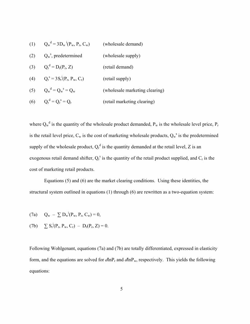
(1) Qwd = 3Dw

i(Pw, Pr, Cw) (wholesale demand)

(2) Qws, predetermined (wholesale supply)

(3) Qrd = Dr(Pr, Z) (retail demand)

(4) Qrs = 3Sr

i(Pr, Pw, Cr) (retail supply)

(5) Qwd = Qw

s = Qw (wholesale marketing clearing)

(6) Qrd = Qr

s = Qr (retail marketing clearing)

where Qwd is the quantity of the wholesale product demanded, Pw is the wholesale level price, Pr

is the retail level price, Cw is the cost of marketing wholesale products, Qws is the predetermined

supply of the wholesale product, Qrd is the quantity demanded at the retail level, Z is an

exogenous retail demand shifter, Qrs is the quantity of the retail product supplied, and Cr is the

cost of marketing retail products.

Equations (5) and (6) are the market clearing conditions. Using these identities, the

structural system outlined in equations (1) through (6) are rewritten as a two-equation system:

(7a) Qw – ∑ Dwi(Pw, Pr, Cw) = 0,

(7b) ∑ Sri(Pr, Pw, Cr) – Dr(Pr, Z) = 0.

Following Wohlgenant, equations (7a) and (7b) are totally differentiated, expressed in elasticity

form, and the equations are solved for dlnPr and dlnPw, respectively. This yields the following

equations:

5

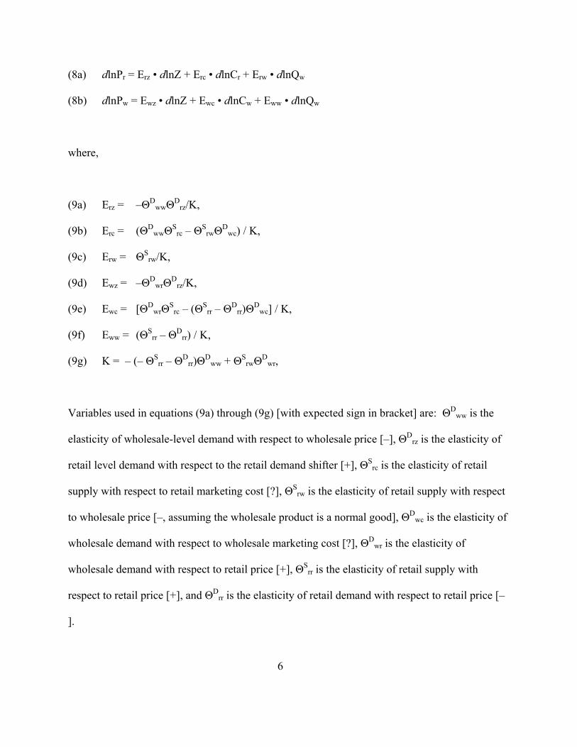
(8a) dlnPr = Erz • dlnZ + Erc • dlnCr + Erw • dlnQw

(8b) dlnPw = Ewz • dlnZ + Ewc • dlnCw + Eww • dlnQw

where,

(9a) Erz = –ΘDwwΘD

rz/K,

(9b) Erc = (ΘDwwΘS

rc – ΘSrwΘD

wc) / K,

(9c) Erw = ΘSrw/K,

(9d) Ewz = –ΘDwrΘD

rz/K,

(9e) Ewc = [ΘDwrΘS

rc – (ΘSrr – ΘD

rr)ΘDwc] / K,

(9f) Eww = (ΘSrr – ΘD

rr) / K,

(9g) K = – (– ΘSrr – ΘD

rr)ΘDww + ΘS

rwΘDwr,

Variables used in equations (9a) through (9g) [with expected sign in bracket] are: ΘDww is the

elasticity of wholesale-level demand with respect to wholesale price [–], ΘDrz is the elasticity of

retail level demand with respect to the retail demand shifter [+], ΘSrc is the elasticity of retail

supply with respect to retail marketing cost [?], ΘSrw is the elasticity of retail supply with respect

to wholesale price [–, assuming the wholesale product is a normal good], ΘDwc is the elasticity of

wholesale demand with respect to wholesale marketing cost [?], ΘDwr is the elasticity of

wholesale demand with respect to retail price [+], ΘSrr is the elasticity of retail supply with

respect to retail price [+], and ΘDrr is the elasticity of retail demand with respect to retail price [–

].

6

Using the signs assigned to the elasticities listed in equations (9a) through (9g), it is

possible to sign the parameters of equations (8a) and (8b). Given that K is negative, Erz is

negative, Erw is positive, Ewz is positive, Eww is negative, and Erc and Ewc cannot be assigned

signs because the signs of ΘSrc and ΘD

wc are ambiguous.

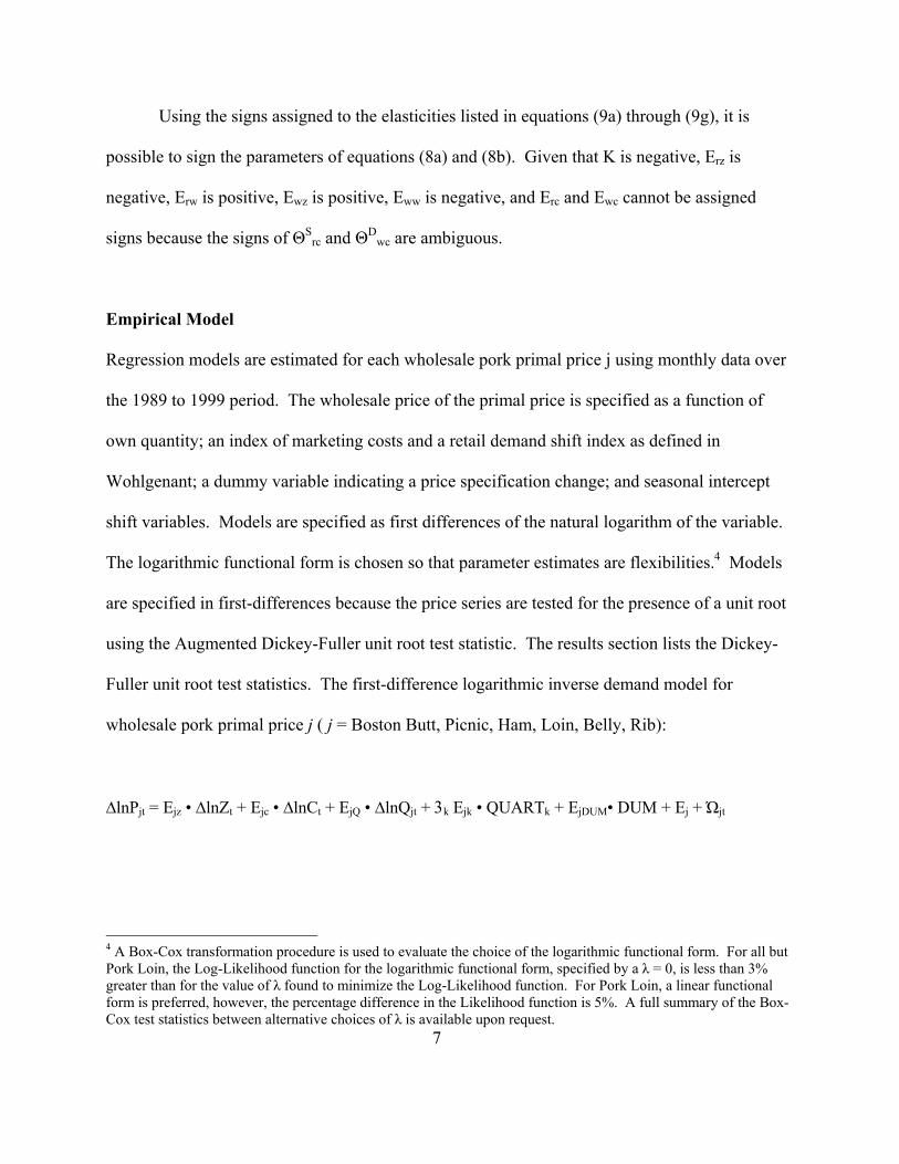
Empirical Model

Regression models are estimated for each wholesale pork primal price j using monthly data over

the 1989 to 1999 period. The wholesale price of the primal price is specified as a function of

own quantity; an index of marketing costs and a retail demand shift index as defined in

Wohlgenant; a dummy variable indicating a price specification change; and seasonal intercept

shift variables. Models are specified as first differences of the natural logarithm of the variable.

The logarithmic functional form is chosen so that parameter estimates are flexibilities.4 Models

are specified in first-differences because the price series are tested for the presence of a unit root

using the Augmented Dickey-Fuller unit root test statistic. The results section lists the Dickey-

Fuller unit root test statistics. The first-difference logarithmic inverse demand model for

wholesale pork primal price j ( j = Boston Butt, Picnic, Ham, Loin, Belly, Rib):

∆lnPjt = Ejz • ∆lnZt + Ejc • ∆lnCt + EjQ • ∆lnQjt + 3k Ejk • QUARTk + EjDUM• DUM + Ej + Ώjt

7

4 A Box-Cox transformation procedure is used to evaluate the choice of the logarithmic functional form. For all but Pork Loin, the Log-Likelihood function for the logarithmic functional form, specified by a λ = 0, is less than 3% greater than for the value of λ found to minimize the Log-Likelihood function. For Pork Loin, a linear functional form is preferred, however, the percentage difference in the Likelihood function is 5%. A full summary of the Box-Cox test statistics between alternative choices of λ is available upon request.

Variable definitions and summary statistics of data used to estimate equation (10) are listed in

table 1. The data section following this section describes the data in more detail. Equation (10)

states that variability in monthly wholesale pork primal price is a function of a retail demand

shift index (Z), a marketing cost index (C), own-quantity of primal cut j (Q), a 0 or 1 binary

seasonal variable (QUART), a 0 or 1 binary variable to represent the change in price quote

effective January 1998 (DUM), and a constant (E). Ώwit is a random disturbance term. The

dummy variable for the change in price quote is set equal to 1 for January 1998 and 0 otherwise.

For the retail demand shifter, Wohlgenant suggests totally differentiating the retail

demand for the jth primal and allowing the retail demand shift variable to equal the residual of

the left hand side (dlnQj) less the own-price elasticity multiplied by the differentiated logarithm

of the own-price (ejj•dlnPj). Thus, following Wohlgenant, the retail demand shifter specified for

this study is of the form:

(10) ∆lnZt = 3l ejl • ∆lnPrlt + ejy • ∆lnYt + ∆lnPOPt ,

where ejl is the cross-price elasticity of competing meat l, ejy is the income elasticity of meat j

(pork here), Prlt is the retail price (r) of meat l and time t, Yt is per capita income at time t, and

POPt is the resident population at time t.

To determine whether the own-quantity flexibility varies seasonally, a slight modification

is made to the model specified in equation (10). An interaction term between the own-quantity

variable and the quarterly shift variable is constructed. This allows for the estimation of

quarterly own-quantity flexibility estimates for each wholesale primal cut j. The specification of

this model is: 8

(12) ∆lnPjt = Ejz•∆lnZt + Ejc•∆lnCt + 3k EjkQ•∆lnQjt•QUARTk + 3k Ejk•QUARTk + EjDUM•DUM + Ew + Ώjt ,

where variable definitions for equation (12) are the same as above.

Evaluating a Change in Wholesale Primal Demand

The test of model stability, i.e., parameter stability, used for this analysis is the Flexible

Least Squares (FLS) estimator. Tesfatsion and Veitch, and Dorfman and Foster provide an

extensive explanation of the FLS estimator. FLS detects parameter instability that may indicate

possible structural change in the analyzed variable. Tests for structural change, e.g., CUSUM,

Chow, and Recursive residual tests, provide researchers an indication of where to partition the

data. These methods, however, do not show the rate at which structural change occurs, the

length of occurrence when there is a temporary structural change, and partitioning the data can

cause degrees of freedom problems when using a small sample size.

Graphically depicting how the wholesale own-quantity flexibility changes over time can

be useful in assessing structural change and the FLS estimator allows for such a graphical

representation. The graphical representation makes inferences regarding potential structural

changes that may cause the own-quantity flexibility estimate to change over time or temporarily.

The FLS estimator briefly is described here. Assume a simple aggregate inverse

wholesale pork demand model:

(13) P Qt t pork t t= +β ε, ,

where Pt is the wholesale price at time t (t = 1, . . ., T), Qpork,t is the demand for wholesale pork at

time t, and εt is a random disturbance term. The coefficient on wholesale pork demand (βt) is a T

9

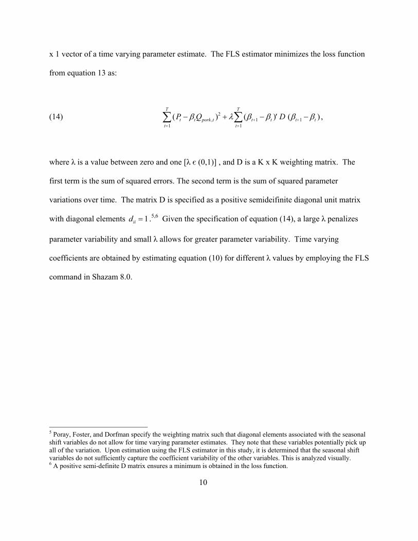
x 1 vector of a time varying parameter estimate. The FLS estimator minimizes the loss function

from equation 13 as:

(14) , ( ) ( ) (,P Q Dt t pork tt

T

t t t tt

T

− + − ′ −=

+ +=

∑ ∑β λ β β β β2

11 1

1

)

where λ is a value between zero and one [λ є (0,1)] , and D is a K x K weighting matrix. The

first term is the sum of squared errors. The second term is the sum of squared parameter

variations over time. The matrix D is specified as a positive semideifinite diagonal unit matrix

with diagonal elements .dii = 1 5,6 Given the specification of equation (14), a large λ penalizes

parameter variability and small λ allows for greater parameter variability. Time varying

coefficients are obtained by estimating equation (10) for different λ values by employing the FLS

command in Shazam 8.0.

5 Poray, Foster, and Dorfman specify the weighting matrix such that diagonal elements associated with the seasonal shift variables do not allow for time varying parameter estimates. They note that these variables potentially pick up all of the variation. Upon estimation using the FLS estimator in this study, it is determined that the seasonal shift variables do not sufficiently capture the coefficient variability of the other variables. This is analyzed visually. 6 A positive semi-definite D matrix ensures a minimum is obtained in the loss function.

10

Data

Averages and standard deviations of data used in the estimation of inverse wholesale pork primal

demand models are listed in table 1. All series are monthly data from February 1989 through

December 1999. LMIC provided the monthly wholesale primal prices for Pork Loin, Pork Rib,

Boston Butt, Ham, Pork Belly, and Boneless Picnic. Price series are represented graphically in

graphs 1, 2, and 3.

Average daily per capita pork consumption for the different meat types is calculated as

pork production adjusted for pork imports, exports, and the between month change in cold

storage stocks for the specific wholesale pork primal. LMIC also supplied the production,

import, and export data. USDA Cold Storage reports provided cold storage stocks information.

For Pork Rib, cold storage values were not kept during the entire time period. Thus, constant

proportions are assumed between pork production and the quantity of Pork Rib in the wholesale

marketplace. Average daily pork consumption between the six different wholesale primals only

varies by the difference in beginning and ending cold storage stocks within the month.

Previous research either assumed fixed proportions between the farm and wholesale level

(Lusk et al. and Parcell and Pierce) or suggested fixed proportions as a result of estimated

models (Capps et al.). Previous research analyzing the fixed proportions hypothesis between

levels in the meat marketing chain are mixed, e.g., Hahn and Green; Wohlgenant, Wohlgenant

and Haidacher. The current study uses a combination of the fixed proportion assumption

(aggregate pork production) and variable proportion assumption (change in cold storage stocks

for individual pork primals) to formulate a daily per capita own-quantity demand variable.

The food marketing cost index is obtained from various issues of Agricultural Outlook.

The retail shift index is computed using national monthly average retail prices for pork chicken,

11

ground beef, and steak (LMIC). Monthly annualized U.S. population and monthly annualized

U.S. disposable income was obtained from the St. Louis Federal Reserve Bank.

Price and index data used for this analysis are nominal values. Following research by

Peterson and Tomek that suggested deflating may cause autocorrelation and introduce a

deterministic trend in the error vector, nominal values are used so to not introduce noise into the

model.7

Results

Each wholesale primal price, after being transformed by the natural logarithm operator, is tested

for stationarity using the augmented Dickey-Fuller, and the lag order is determined by

minimizing the Akaike Information Criteria. The Dickey-Fuller test statistic was –1.61 for Pork

Loin, -1.89 for Boston Butt, -1.55 for Pork Rib, -1.05 for Ham, -2.01 for Pork Belly, -2.82 for

Boneless Picnic, and the 10% critical value is -2.57. Therefore, the null-hypothesis of a unit root

cannot be rejected for five of the six price series. Data are first differenced, and the first

differenced price series are found to be stationary for all of the primal price series. The number

of observations used in the estimation is 131.

12

7 One reviewer expressed concern over the use of nominal values. Peterson and Tomek suggested the use of real price data could result in inefficient standard errors. Thus, as further support for the use of nominal values, a J test was conducted between the nominal price model and a real price model. For H1: nominal prices are appropriate, the p-values for the null-hypothesis of alpha value equal to zero were 0.165 for Pork Loin, 0.499 for Boston Butt, 0.439 for Pork Rib, 0.774 for Ham, 0.905 for Pork Belly, and 0.463 for Boneless Picnic. For H2: real prices are appropriate, the p-values for the null-hypothesis of alpha value equal to zero were 0.167 for Pork Loin, 0.502 for Boston Butt, 0.420 for Pork Rib, 0.775 for Ham, 0.955 for Pork Belly, and 0.482 for Boneless Picnic. The results of the J test, albeit a relative weak test, indicate that either nominal or real prices could be used without loss of efficiency.

Since wholesalers and retailers trade in all wholesale primals, exogenous shocks may

have a similar impact across the wholesale pork primal prices. A Breusch-Pagan test statistic

(table 2) is computed to test for a diagonal covariance matrix. The null-hypothesis of a diagonal

covariance matrix is rejected. Thus, models are estimated using Seemingly Unrelated

Regression (SUR) estimator to improve estimation efficiency (Greene). Durbin-Watson test

statistics for the presence of autocorrelation, an inherent problem with time series data, are listed

at the bottom of table (2). The size of the Durbin -Watson test statistic, for each model, suggests

autocorrelation is not a concern.

As previously stated, the supply of pork is assumed predetermined. To verify this

assumption a test of exogeneity is carried out using the Wald test Statistic (Greene). The statistic

is distributed chi-squared with one degree of freedom, the critical value is 3.84 at the 5% level.

An instrument is computed for the per capita consumption variable by using all other exogenous

variables listed in equation 11 and a lagged per capita consumption variable for the individual

primal (Greene). For each of the test statistics computed, the null-hypothesis of the pork primal

per-capita consumption exogenous to the model cannot be rejected. Each of the test statistic

values is below one. 8

Results of equation (10) are described in table 2. The explanatory variables explain

between 86% and 98% of the variation in the different wholesale pork primal prices, as indicated

by the R2. Because the model is estimated in first-differences of the natural logarithm of the

data, coefficients are flexbilities.

8 Care is taken in the interpretation of the Wald test statistic for endogeneity as it is not considered a powerful test. However, the level of the test statistics computed here – below one – provides a strong argument that a more powerful test statistic will produce a similar result.

13

Own-quantity price flexibility of demand is statistically significant and of the expected

sign for four of the six wholesale primal cuts. Pork Loin and Boston Butt have price flexibility

of demand estimates around –0.49, and Pork Belly and Boneless Picnic have price flexibility of

demand estimates of around –0.25. These four primals represent roughly 55% of the wholesale

carcass value. This result is consistent with the difference between relatively higher valued cuts

and lower valued cuts found for other meat wholesale cuts (Capps et. al.; Lusk et. al.; Parcell and

Pierce). Neither the Pork Rib or Ham price flexibility of demand is statistically significant.

There is not a wholesale price response associated with a change in the quantity demanded for

these products. The size of the price flexibility of demand for the different primals is

significantly different than the aggregate price flexibility of demand estimated by Hahn and

Green, -0.06. This suggests that it may be important to analyze wholesale pork primal prices

separately because aggregation estimation results are not representative of estimation results

obtained for individual primal cuts.

14

A one percent increase in the marketing cost index does not have a statistically significant

impact on any of the wholesale pork primal prices. Hahn and Green also did not find the

marketing cost index to be statistically significant in explaining the variability of the aggregate

wholesale primal price. Visually observing the data indicates that there is little variability in the

food marketing cost index over the period of study.

The retail demand shift variable is statistically significant for three of the six equations.

Furthermore, the sign on the coefficient, when statistically significant, is of the expected sign.

The retail shift index is the largest in magnitude for the Pork Rib and Ham, which suggests Pork

Rib and Ham are more responsive to exogenous changes at the retail level than from a change in

own-quantity demanded at the wholesale level. Because the primary focus of this study is on

determining seasonal variability and changes over time in the price flexibility of demand, the

retail shift index coefficient is not decomposed.

The dummy variable for the change in specification of the USDA wholesale primal price

is not statistically significant for any of the wholesale pork primal price equations. Even though

there is a noticeable change in the price level for each pork primal price, transforming the price

data using natural logarithms and first differences likely reduces the impact of the price quote

specification change in the multivariate analysis.

For the quarterly intercept shift variables, statistical significance and magnitude of the

effect varies by wholesale primal cut. Relative to the first quarter, the price for four of the six

pork primals is statistically lower during the fourth quarter. This is consistent with the

exogenous increase in pork production associated with the seasonal production of pork.

15

Seasonal Variation in Own-Flexibilities

Estimated results of equation (12) are listed in table 3. Equation (12) is specified so that the

price flexibility of demand varies between quarters of the year. Results presented in table 3 only

differ from table 2 by the inclusion of the price flexibility of demand and seasonal shift

interaction terms. Models are estimated jointly using the SUR estimator. The Durbin-Watson

test statistics indicate that residual autocorrelation is not a concern. The explanatory variables

explained between 86% and 98% of the variability in the wholesale pork primal prices over the

period evaluated.

For Pork Loin, Boston Butt, and Boneless Picnic, seasonal varying price flexibility of

demand estimates generally are statistically different from zero. Additionally, a paired t-statistic

is computed between the price flexibility of demand for the respective primal, reported in table 2,

and for each of the statistically significant seasonal varying own-quantity flexibilities, reported in

table 3. For each of the statistically significant price flexibilities of demand reported in table 3,

the calculated paired t-statistic rejects the null-hypothesis that the parameter estimates are equal.9

Thus, the price flexibility of demand for some wholesale pork primals varies within the year.

This result is consistent with the findings of Lusk et al. for the case of Choice and Select beef.

16

9 For Pork Loin, the test statistic for test of means was 7.88, 1.83, 5.92, and 1.01 for the first, second, third, and fourth quarter, respectively. For Boneless Butt, the test statistic for test of means was 3.52, 3.02, and 0.47 for the first, second, and fourth quarter, respectively. For Boneless Picnic, the test statistic for test of means was 9.99 and 3.12 for the first and second quarter, respectively. Statistical significance follows from the t-statistic critical values.

Time Path of Wholesale Primal Flexibilities

Flexible Least Squares is used to graphically represent the time path of the different pork primal

price flexibilities of demand over time. The FLS estimator estimates the model specified in

equation (10). Summary statistics of the flexible least squares estimator for the own-quantity

flexibility coefficients are reported in table 4 for chosen values of λ equal to 0.001, 0.1 and 1. As

λ becomes larger, the Flexible Least Squares estimator approaches the OLS estimator and the

standard errors on the coefficient decrease in value rapidly.

The time paths of the price flexibility of demand estimates for Boston Butt, Boneless

Picnic, Pork Belly, Ham, and Pork Loin, at λ=0.001, are graphed in figure 4. The weighting

coefficient, λ=0.001, is chosen to give the model the most flexibility. As observed from figure 4,

the price flexibility of demand remained fairly constant for all cuts until 1997. Following the

beginning of 1997, the wholesale primal flexibilities, other than Pork Belly and Ham, became

significantly more flexible (increased in absolute value), particularly during 1998.

For Boston Butt, the price flexibility of demand is observed to be five times greater in

absolute value than historically observed. Alternatively, the price flexibility of demand for Pork

Belly and Ham is relatively unchanged, or increases slightly, over the entire period. One

assessment of why the wholesale Pork Belly and Ham price flexibility of demand is unchanged

stems from cold storage stocks of Pork Belly and Ham. Specifically, cold storage stocks of Pork

Belly and Ham increases so that a change in price is not needed to offset the greater quantity of

pork moving through the wholesale marketplace. Figure 5 graphically depicts the time path of

the Ham price flexibility of demand and cold storage stocks.

Given the price flexibility of demand estimates began increasing (in absolute value) in

1997, not all of the change is attributed to the large supply of hogs entering the market in 1998.

17

Demand factors such as advertising campaigns, change in consumer diet, case-ready and branded

products possibly led to this change. Unfortunately, given the limited time period from which

the structural change occurred, finding strong conclusions about the cause of the change is

difficult. However, this analysis motivates the need for further analysis in the future.

Conclusions

Inverse wholesale pork primal demand models, for Pork Loin, Boston Butt, Pork Rib, Ham, Pork

Belly, and Boneless Picnic, are estimated to empirically analyze whether there is a seasonal

component of the wholesale price flexibility of demand and to determine whether the own-

quantity flexibility increases in magnitude (absolute value). The period of evaluation is 1989

through 1999. No previous research explicitly analyzes factors affecting variability in wholesale

pork primal prices. Results indicate that the price flexibility of demand varies by wholesale

primal; there is seasonal variation in the own-quantity flexibility of Pork Loin, Boston Butt, and

Boneless Picnic; and the price flexibility of demand for Pork Loin, Boston But, and Boneless

Picnic increases in magnitude (absolute value) over time. These primals account for

approximately 55% of the wholesale pork carcass. Demand factors such as advertising

campaigns, change in consumer diet, case-ready and branded products may have lead to this

change. Conversely, some observed change in price flexibility of demand possibly resulted from

the over supply of hogs entering the market during the fourth quarter of 1998. However, the

observed magnitude change in price flexibility of demand is significantly less than the level of

the absolute decrease in live hog price flexibility of demand observed in the Fall of 1998

(Parcell, Mintert, and Plain).

18

For Pork Loin, Boston Butt, and Boneless Picnic, the estimated first quarter price

flexibility of demand is greater than twice the magnitude of the estimated price flexibility of

demand when not accounting for seasonal fluctuations. During other periods within the year, the

difference in magnitude is less. The price flexibility of demand for Boston Butt was found to

have increased in magnitude by about five times during the past two years, -0.30 to around –

1.50. However, the price flexibility of demand of Pork Belly and Ham was either unchanged or

increased over the period of study. One reason for this may be the relatively longer period that

Pork Bellies and Ham can remain in cold storage, thus, allowing cold storage stocks to change

and off-set large price fluctuations.

Results of this study are important for two specific reasons. First, the disaggregated price

flexibilities of demand estimated in this study are significantly different than aggregate

wholesale price flexibility of demand estimated in previous research. Second, the results of this

study suggest there is seasonal variability in the magnitude of a wholesale primal price response

from a corresponding one percent change in quantity demanded. This result is important because

it provides processors with information on pricing strategies, helps processors make better

quarterly cash flow and income projections, and suggests that future research analyzing

structural change and market power needs to consider seasonality. Lastly, this study uses

parametric analysis to validate claims that the own-quantity flexibility at the wholesale level

increased in magnitude over time. However, the change in own-quantity flexibility magnitude is

not necessarily apparent or consistent across wholesale pork primals.

As with all studies, this study has limitations. First, separability among the wholesale

pork primals is assumed due to data limitations common with analysis of this type. Secondly, a

proxy variable is computed as an own-quantity for different pork primals. Numerous researchers

19

test the assumption of fixed proportions; however, Hahn and Green noted that most tests are

indirect. Future research could empirically test the fixed proportion hypothesis by using cold

storage stocks of individual pork primals as a proxy for own-quantity versus pork production at

the farm level.

20

References

Capps, O., Jr., D.E. Farris, P.J. Byrne, J.C. Namken, and C.D. Lambert. “Determinants of Wholesale Beef-Cut Prices.” Journal of Agriculture and Applied Economics 26(July 1994):183-99.

Dorfman, J. and K. Foster. “Estimating Productivity Change with Flexible Coefficients.”

Western Journal of Agricultural Economics 16(1991):280-90. Federal Reserve Economic Data. "Annual U.S. Population." Federal Reserve Bank of St. Louis,

Downloaded from Internet at: www.stls.frb.org, January 2000. ____________. "U.S. Total Disposable Income." Federal Reserve Bank of St. Louis,

Downloaded from Internet at: www.stls.frb.org, January 2000. Greene, W.H. Econometric Analysis. Englewood Cliffs, NJ: Macmillan, 1993. Grimes, G., and S. Meyer. "Hog Marketing Contract Study." University of Missouri and

National Pork Producers Council, January 2000, http://agebb.missouri.edu/mkt/vertstud.ht

Goodwin, B., and M. Holt. “Price Transmission and Asymmetry Adjustment in the U.S. Beef

Sector.” American Journal of Agricultural Economics. 81(1999): 630-37. Livestock Marketing Information Center. Data obtained via Internet download, May 2000.

http://lmic1.co.nrcs.usda.gov. Lusk, J.L., T.L. Marsh, T.C. Schroeder, and J. A. Fox. “Wholesale Demand for USDA Quality

Graded Boxed Beef and Effects of Seasonality.” Paper presented at the Western Agricultural Economics Association Meetings, Vancouver, British Columbia, June, 2000.

Lutkepohl, H. "The Source of the U.S. Money Demand Instability." Empirical Economics,

18(1993):729-43. McGuirk, A., P. Driscoll, J. Alwang, and H. Huang. "System Misspecification Testing and

Structural Change in the Demand for Meats." Journal of Agricultural and Resource Economics 20(1995):1-21.

National Pork Producers Council. "Pork producer economic recovery plan presented." News . . .

from the Nation's Pork Industry, July 21, 1999 (www.nppc.org/NEWS) Parcell, J.L, J. Mintert, and R. Plain. “An Empirical Examination of Live Hog Demand”

Presented paper at NCR-134 Conference on Applied Commodity Price Analysis, Forecasting, and Market Risk Management, ed. T.C. Schroeder, pp. 1-22. Department of Agricultural Economics, Kansas State University, 2000.

21

Parcell, J.L., and V. Pierce. “Seasonality in Wholesale Poultry Prices.” Journal of Agricultural

and Applied Economics, Forthcoming December 2000. Plain, R., and G. Grimes. National Hog Farmer, April 1999. Peterson, H.H., and W.G. Tomek. “Implications of Deflating Commodity Prices for Time-Series

Analysis.” Presented paper at NCR-134 Conference on Applied Commodity Price Analysis, Forecasting, and Market Risk Management, ed. T.C. Schroeder, pp. 1-25. Department of Agricultural Economics, Kansas State University, 2000.

Schroeder, T.C., and J. Mintert. “Linkages in Weekly and Monthly Live Hog, Wholesale, Pork,

and Retail Pork Prices.” Report Prepared for the National Pork Producers Council, December 1996.

SHAZAM. Econometrics Computer Program Users Reference Manual, Version 8.0. New

York, NY, McGraw Hill, 1993. Spivey, S.E., V. Salin, and D. Anderson. “Analysis of the Effect of Packing Capacity on Hog

Prices.” Selected Paper Presented at the Meetings of the Southern Agricultural Economics Association, Lexington, KY, 2000.

Tesfatsion, L., and J. Veitch. "U.S. Money Demand Instability", Journal of Economic Dynamics

and Control 14(1990): 151-73. Tomek, W. "Limits on Price Analysis." American Journal of Agricultural Economics.

67(1985): 905-1015. United States Department of Agriculture, Economic Research Service. "Agricultural Outlook."

Various issues, 1989 - 1999. ____________. Economic Research Service. "Cold Storage Reports." Various issues, 1989 -

1999. Wohlgenant, M.K. "Demand for Farm Output in a Complete System of Demand Functions."

American Journal of Agricultural Economics, 71(1989): 241-52. Wohlgenant, M.K., and R.C. Haidacher. Retail to Farm Linkages for a Complete Demand

System of Food Commodities. Tech. Bull. No. 1175, USDA/Economic Research Service, Washington DC, 1989

22

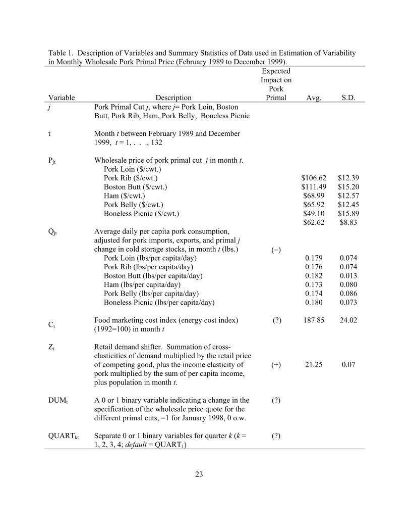
Table 1. Description of Variables and Summary Statistics of Data used in Estimation of Variability in Monthly Wholesale Pork Primal Price (February 1989 to December 1999). Variable

Description

Expected Impact on

Pork Primal

Avg.

S.D. j Pork Primal Cut j, where j= Pork Loin, Boston

Butt, Pork Rib, Ham, Pork Belly, Boneless Picnic

t Month t between February 1989 and December

1999, t = 1, . . ., 132

Pjt

Wholesale price of pork primal cut j in month t. Pork Loin ($/cwt.) Pork Rib ($/cwt.) Boston Butt ($/cwt.) Ham ($/cwt.) Pork Belly ($/cwt.) Boneless Picnic ($/cwt.)

$106.62 $111.49 $68.99 $65.92 $49.10 $62.62

$12.39 $15.20 $12.57 $12.45 $15.89 $8.83

Qjt

Average daily per capita pork consumption, adjusted for pork imports, exports, and primal j change in cold storage stocks, in month t (lbs.) Pork Loin (lbs/per capita/day) Pork Rib (lbs/per capita/day) Boston Butt (lbs/per capita/day) Ham (lbs/per capita/day) Pork Belly (lbs/per capita/day) Boneless Picnic (lbs/per capita/day)

(−)

0.179 0.176 0.182 0.173 0.174 0.180

0.074 0.074 0.013 0.080 0.086 0.073

Ct

Food marketing cost index (energy cost index) (1992=100) in month t

(?)

187.85 24.02

Zt

Retail demand shifter. Summation of cross-elasticities of demand multiplied by the retail price of competing good, plus the income elasticity of pork multiplied by the sum of per capita income, plus population in month t.

(+)

21.25

0.07

DUMt A 0 or 1 binary variable indicating a change in the specification of the wholesale price quote for the different primal cuts, =1 for January 1998, 0 o.w.

(?)

QUARTkt

Separate 0 or 1 binary variables for quarter k (k = 1, 2, 3, 4; default = QUART1)

(?)

23

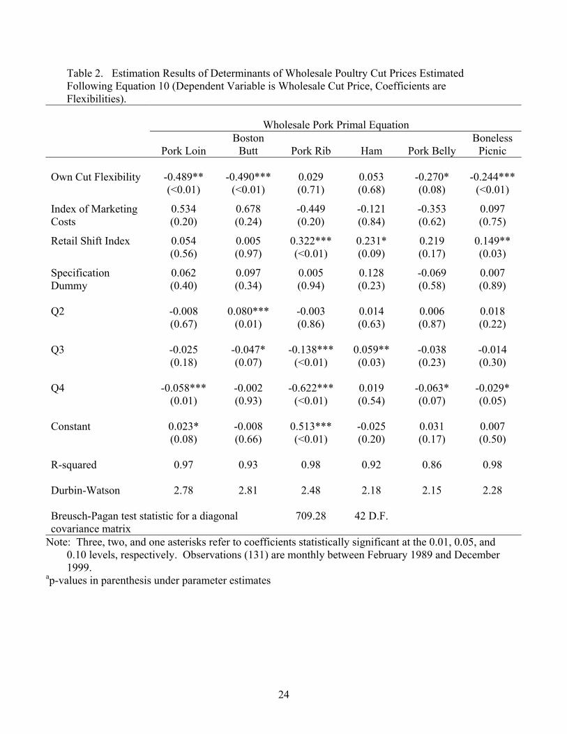
Table 2. Estimation Results of Determinants of Wholesale Poultry Cut Prices Estimated Following Equation 10 (Dependent Variable is Wholesale Cut Price, Coefficients are Flexibilities).

Wholesale Pork Primal Equation

Pork Loin

Boston Butt

Pork Rib

Ham

Pork Belly

Boneless Picnic

Own Cut Flexibility

-0.489** (<0.01)

-0.490***

(<0.01)

0.029 (0.71)

0.053 (0.68)

-0.270* (0.08)

-0.244***

(<0.01)

Index of Marketing Costs

0.534 (0.20)

0.678 (0.24)

-0.449 (0.20)

-0.121 (0.84)

-0.353 (0.62)

0.097 (0.75)

Retail Shift Index

0.054 (0.56)

0.005 (0.97)

0.322*** (<0.01)

0.231* (0.09)

0.219 (0.17)

0.149** (0.03)

Specification Dummy

0.062 (0.40)

0.097 (0.34)

0.005 (0.94)

0.128 (0.23)

-0.069 (0.58)

0.007 (0.89)

Q2

-0.008 (0.67)

0.080*** (0.01)

-0.003 (0.86)

0.014 (0.63)

0.006 (0.87)

0.018 (0.22)

Q3

-0.025 (0.18)

-0.047* (0.07)

-0.138*** (<0.01)

0.059** (0.03)

-0.038 (0.23)

-0.014 (0.30)

Q4

-0.058*** (0.01)

-0.002 (0.93)

-0.622*** (<0.01)

0.019 (0.54)

-0.063* (0.07)

-0.029* (0.05)

Constant

0.023* (0.08)

-0.008 (0.66)

0.513*** (<0.01)

-0.025 (0.20)

0.031 (0.17)

0.007 (0.50)

R-squared 0.97 0.93 0.98 0.92 0.86 0.98 Durbin-Watson 2.78 2.81 2.48 2.18 2.15 2.28 Breusch-Pagan test statistic for a diagonal covariance matrix

709.28 42 D.F.

Note: Three, two, and one asterisks refer to coefficients statistically significant at the 0.01, 0.05, and 0.10 levels, respectively. Observations (131) are monthly between February 1989 and December 1999.

ap-values in parenthesis under parameter estimates

24

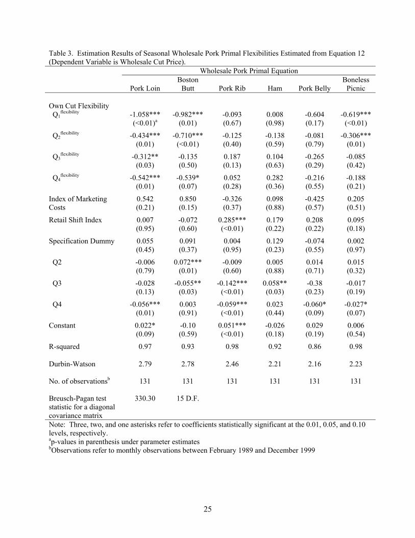
Table 3. Estimation Results of Seasonal Wholesale Pork Primal Flexibilities Estimated from Equation 12 (Dependent Variable is Wholesale Cut Price).

Wholesale Pork Primal Equation

Pork Loin Boston

Butt

Pork Rib

Ham

Pork Belly Boneless

Picnic Own Cut Flexibility

Q1flexibility

-1.058*** (<0.01)a

-0.982*** (0.01)

-0.093 (0.67)

0.008 (0.98)

-0.604 (0.17)

-0.619*** (<0.01)

Q2flexibility

-0.434*** (0.01)

-0.710*** (<0.01)

-0.125 (0.40)

-0.138 (0.59)

-0.081 (0.79)

-0.306*** (0.01)

Q3flexibility

-0.312** (0.03)

-0.135 (0.50)

0.187 (0.13)

0.104 (0.63)

-0.265 (0.29)

-0.085 (0.42)

Q4flexibility

-0.542*** (0.01)

-0.539* (0.07)

0.052 (0.28)

0.282 (0.36)

-0.216 (0.55)

-0.188 (0.21)

Index of Marketing Costs

0.542 (0.21)

0.850 (0.15)

-0.326 (0.37)

0.098 (0.88)

-0.425 (0.57)

0.205 (0.51)

Retail Shift Index

0.007 (0.95)

-0.072 (0.60)

0.285*** (<0.01)

0.179 (0.22)

0.208 (0.22)

0.095 (0.18)

Specification Dummy

0.055 (0.45)

0.091 (0.37)

0.004 (0.95)

0.129 (0.23)

-0.074 (0.55)

0.002 (0.97)

Q2

-0.006 (0.79)

0.072*** (0.01)

-0.009 (0.60)

0.005 (0.88)

0.014 (0.71)

0.015 (0.32)

Q3

-0.028 (0.13)

-0.055** (0.03)

-0.142*** (<0.01)

0.058** (0.03)

-0.38 (0.23)

-0.017 (0.19)

Q4

-0.056*** (0.01)

0.003 (0.91)

-0.059*** (<0.01)

0.023 (0.44)

-0.060* (0.09)

-0.027* (0.07)

Constant

0.022* (0.09)

-0.10 (0.59)

0.051*** (<0.01)

-0.026 (0.18)

0.029 (0.19)

0.006 (0.54)

R-squared 0.97 0.93 0.98 0.92 0.86 0.98 Durbin-Watson 2.79 2.78 2.46 2.21 2.16 2.23 No. of observationsb 131 131 131 131 131 131 Breusch-Pagan test statistic for a diagonal covariance matrix

330.30 15 D.F.

Note: Three, two, and one asterisks refer to coefficients statistically significant at the 0.01, 0.05, and 0.10 levels, respectively. ap-values in parenthesis under parameter estimates bObservations refer to monthly observations between February 1989 and December 1999

25

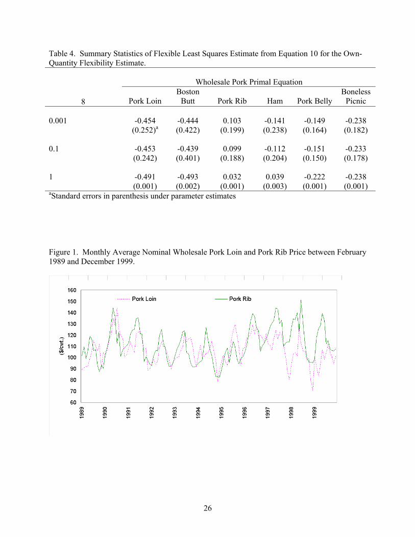
Table 4. Summary Statistics of Flexible Least Squares Estimate from Equation 10 for the Own-Quantity Flexibility Estimate.

Wholesale Pork Primal Equation

8

Pork Loin

Boston Butt

Pork Rib

Ham

Pork Belly

Boneless Picnic

0.001 -0.454 -0.444 0.103 -0.141 -0.149 -0.238 (0.252)a (0.422) (0.199) (0.238) (0.164) (0.182) 0.1 -0.453 -0.439 0.099 -0.112 -0.151 -0.233 (0.242) (0.401) (0.188) (0.204) (0.150) (0.178) 1 -0.491 -0.493 0.032 0.039 -0.222 -0.238 (0.001) (0.002) (0.001) (0.003) (0.001) (0.001) aStandard errors in parenthesis under parameter estimates Figure 1. Monthly Average Nominal Wholesale Pork Loin and Pork Rib Price between February 1989 and December 1999.

26

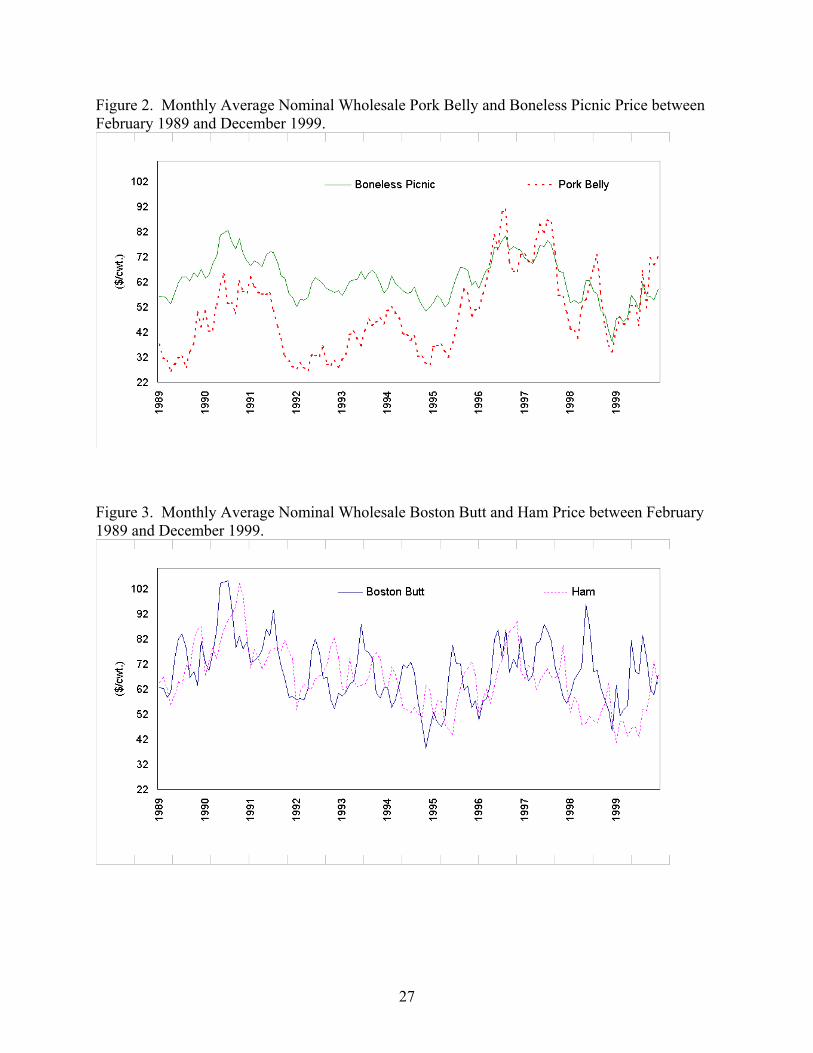
Figure 2. Monthly Average Nominal Wholesale Pork Belly and Boneless Picnic Price between February 1989 and December 1999.

Figure 3. Monthly Average Nominal Wholesale Boston Butt and Ham Price between February 1989 and December 1999.

27

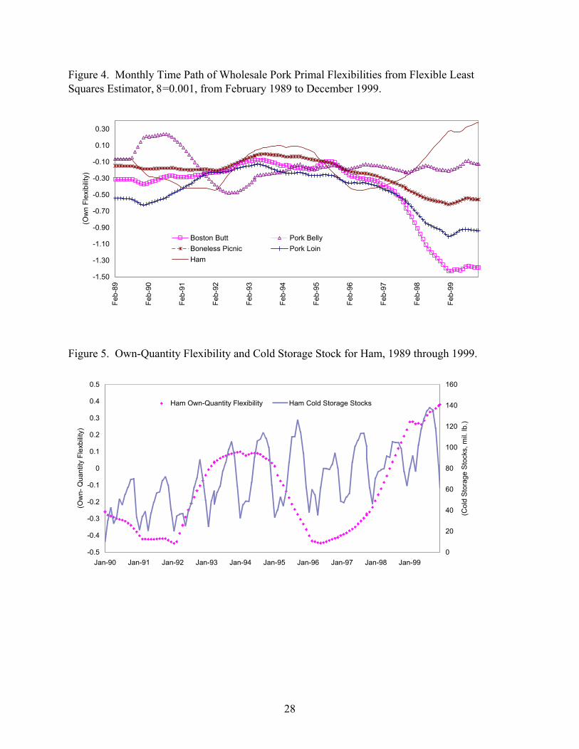
Figure 4. Monthly Time Path of Wholesale Pork Primal Flexibilities from Flexible Least Squares Estimator, 8=0.001, from February 1989 to December 1999.

-1.50

-1.30

-1.10

-0.90

-0.70

-0.50

-0.30

-0.10

0.10

0.30

Feb-

89

Feb-

90

Feb-

91

Feb-

92

Feb-

93

Feb-

94

Feb-

95

Feb-

96

Feb-

97

Feb-

98

Feb-

99

(Ow

n Fl

exib

ility)

Boston Butt Pork BellyBoneless Picnic Pork LoinHam

Figure 5. Own-Quantity Flexibility and Cold Storage Stock for Ham, 1989 through 1999.

-0.5

-0.4

-0.3

-0.2

-0.1

0

0.1

0.2

0.3

0.4

0.5

Jan-90 Jan-91 Jan-92 Jan-93 Jan-94 Jan-95 Jan-96 Jan-97 Jan-98 Jan-99

(Ow

n- Q

uant

ity F

lexb

ility)

0

20

40

60

80

100

120

140

160

(Col

d St

orag

e St

ocks

, mil.

lb.)

Ham Own-Quantity Flexibility Ham Cold Storage Stocks

28