Embed Size (px)
Citation preview

J Sci ComputDOI 10.1007/s10915-017-0448-1
An Efficient Boundary Integral Scheme for the MBOThreshold Dynamics Method via the NUFFT
Shidong Jiang1 · Dong Wang2 · Xiao-Ping Wang2
Received: 25 January 2017 / Revised: 27 April 2017 / Accepted: 2 May 2017© Springer Science+Business Media New York 2017
Abstract The MBO threshold dynamics method consists of two steps. The first step solvesa pure initial value problem of the heat equation with the initial data being the indicatorfunction of some bounded domain. In the second step, the new sharp interface is generatedvia thresholding either by some prescribed solution value or by volume preserving. Wepropose an efficient boundary integral scheme for simulating the threshold dynamics via thenonuniform fast Fourier transform (NUFFT). The first step is carried out by evaluating aboundary integral via the NUFFT, and the second step is performed applying a root-findingalgorithm along the normal directions of a discrete set of points at the interface. Unlike mostexistingmethodswhere volume discretization is needed for thewhole computational domain,our scheme requires the discretization of physical space only in a small neighborhood of theinterface and thus is meshfree. The algorithm is spectrally accurate in space for smoothinterfaces and has O(N log N ) complexity, where N is the total number of discrete pointsnear the interface when the time step �t is not too small. The performance of the algorithmis illustrated via several numerical examples in both two and three dimensions.
Keywords Threshold dynamics · Nonuniform FFT · MBO method · Heat equation ·Motion by mean curvature
Mathematics Subject Classification 35K05 · 65M70 · 76T99 · 82C24
B Shidong [email protected]
Dong [email protected]
Xiao-Ping [email protected]
1 Department of Mathematical Sciences, New Jersey Institute of Technology, Newark, NJ 07102,USA
2 Department of Mathematics, The Hong Kong University of Science and Technology,Clear Water Bay, Kowloon, Hong Kong, China
123

J Sci Comput
1 Introduction
Interface motion is an important topic in many areas of applied mathematics and scientificcomputing including fluid mechanics, image processing, and computer vision. Many numer-ical methods have been developed for simulating interface dynamics including front-trackingmethods [21,37], level set methods [9,27,40], and phase field methods [12,39].
In 1992,Merriman,Bence, andOsher (MBO) [24] developed a threshold dynamicsmethodfor the motion of the interface driven by the mean curvature, where the governing equationis Vn(x) = κ(x) with Vn(x) being the normal velocity of a point x on the interface and κ(x)being the mean curvature at x . To be more precise, let D ∈ R
n be a domain whose boundaryΓ = ∂D is to be evolved via motion bymean curvature. For each time step, theMBOmethodgenerates the new interface Γnew (or equivalently, Dnew) via the following two steps:Step 1 Solve the pure initial value problem of the heat equation to obtain its solution u∗ att = �t
ut = �u,
u|t=0 = χD .
Here χD is the indicator function of the domain D, i.e.,
χD(x) ={1, x ∈ D,
0, otherwise.(1)
Step 2 Obtain the domain Dnew by
Dnew ={x : u∗(x,�t) ≥ 1
2
}.
The MBO method converges to continuous motion by mean curvature as �t → 0 [1,2,10].The method has become very popular due to its simplicity and unconditional stability, andthus it has also been extended to handle many other applications. These applications includemulti-phase flows with arbitrary surface tensions [7], area- or volume-preserving interfacemotion [19,35,37], and wetting on solid surfaces [38]. Various algorithms and rigorous erroranalysis have been performed to refine and extend the original MBO method and relatedmethods for the aforementioned problems (see, for example, [3,8,17,18,23,31–33]). Thesealgorithms all consist of two time March ing steps with the same first step as the MBOmethod. Only the second thresholding step of obtaining the new sharp interface is modified.Sometimes it is obtained by finding a level surface of a specific value of the solution tothe heat flow as in the original MBO method; at other times it is obtained by finding thevolume-preserving surface or by minimizing certain functional whose exact form dependson the specific application.
In this paper, we propose an efficient algorithm for the threshold dynamics method withan NUFFT-based heat equation solver. Standard potential theory [11] shows that the solutionto the pure initial value problem of the heat equation is given by the convolution of the heatkernel G(x, y; t) with the initial data u0. The convolution integral on the whole domain canbe converted to a boundary integral by the divergence theorem or Green’s theorem. We firstshow that an equispaced grid is sufficient to obtain a spectral approximation for the heatkernel at a fixed time t = �t . We then apply the NUFFT [4,5,13] to evaluate the boundaryintegral at a set of target points. For threshold dynamics, the interface moves within a bandaround previous positions with a bandwidth of O(
√�t) due to the diffusion process. Thus
we may choose a set of pN points as the target points with N being the number of points
123

J Sci Comput
on the interface and p being the number of points along each normal direction (p is usually10–20). Finally, we use a standard root-finding procedure for thresholding. The algorithmis spectrally accurate in space. It is also very efficient when �t is not too small for threereasons. First, there is no need to discretize the whole computational domain and only pNpoints near the interface are needed in physical space. Second, the NUFFT has the sameO(N log N ) complexity as the standard fast Fourier transform (FFT). Third, the root-findingprocedure converges rapidly, usually in 4–6 iterations to full double precision, thanks to thesmoothing effect of the diffusion process. Our method is also meshfree since it tracks themotion of a set of points only.
Previous work and our contributionsMany excellent numerical methods are available forsimulating threshold dynamics. Instead of presenting a comprehensive review of these meth-ods, we would like to discuss other NUFFT-based methods and explain how they differ fromour method. In [30,32], efficient algorithms are developed for diffusion-generated motionby mean curvature. The algorithms assume Neumann boundary conditions on a rectangularbox, represent the solution to the heat equation with a cosine series, and then use the NUFFTto solve the heat equation on an adaptive grid.
In [14], a spectral approximation of the heat kernel is constructed with uniform absoluteerror for all t > δ. Due to this much stricter requirement, the spectral approximation needsan adaptive nonuniform node in the Fourier space with dyadic refinement towards the origin.In [22], a fast solver is developed to solve the initial value problem of the heat equation usingthe NUFFT based on the adaptive nonuniform approximation of the heat kernel in [14]. Thepaper aims to find the solution for all t > δ and thus assumes that the initial data is smoothand requires time March ing.
In the threshold dynamics method, due to the thresholding step, we only need to findthe solution to the heat equation at t = �t since the diffusion process starts anew for eachtime step. Thus we only need to approximate the heat kernel at t = �t . Our analysis showsthat an equispaced grid in the Fourier space is sufficient to approximate the heat kernel withspectral accuracy. That is, we do not need to use adaptive Gaussian nodes in the Fourierspace as in [14], nor is it necessary to impose Neumann boundary conditions on an artificialrectangular box in order to be able to use the cosine series to represent the solution as in [32].The computational advantages are two fold. First, fewer Fourier modes are needed in theapproximation of the heat kernel. Second, we only need type-1 and type-2 NUFFTs insteadof the much more expensive type-3 NUFFT for evaluating the solution to the heat equationin an arbitrary set of points in physical space.
Another difference is that [22] assumes that the initial data is smooth, while we assumethat it is discontinuous piecewise constant. Thus directly applying the method in [22] woulddecrease the order of accuracy sharply because the Fourier transform of the initial datadecays slowly. We use the divergence theorem or Green’s theorem to reduce the volume orarea integral to a boundary integral, which reduces the dimension of the problem by onewithout sacrificing the high-order feature of the algorithm for smooth or piecewise-smoothboundaries.
We perform the computation either on or near the interface in both the solving stage and thethresholding stage. This makes our algorithm more efficient than the methods in [30,32] andenables it to achieve high order in space more easily. These advantages increase the appealof our algorithm for certain applications in computational fluid dynamics. Our scheme maybe extended to handle topological changes and multiphase flows such as wetting problemsas in [30,32], but that is outside the scope of this paper.
Organization of the paper In Sect. 2, we present an NUFFT-based solver for the initialvalue problem of the heat equation with piecewise constant initial data in both two and
123

J Sci Comput
three dimensions. In Sect. 3, we discuss the thresholding step involving the root-findingprocedure. Section4 contains several numerical examples demonstrating the performance ofthe proposed numerical algorithm. Finally, we conclude the paper with further discussionsand extensions.
2 An NUFFT-Based Solver for the Heat Equation in Free Space
In this section, we consider solving the pure initial value problem of the heat equation:
ut = �u,
u(x, 0) = u0(x) (2)
with the initial data u0 being the indicator function of some bounded domain D ∈ Rd (d =
2, 3). We assume that the boundary ∂D of D is a smooth manifold which is homomorphicto Sd−1 (i.e., the unit circle in R
2 and unit sphere in R3). We are interested in calculating
u(x,�t) for a given set of target points x (for example, in the neighborhood of ∂D) at some�t < 1. Green’s function (or the fundamental solution) of the heat equation in R
d is givenby the formula
Gd(x, y; t) = 1
(4π t)d/2 e−‖x−y‖2/4t , x, y ∈ R
d . (3)
u(x,�t) is given by the formula
u(x,�t) =∫
· · ·∫Rd
Gd(x, y;�t)u0(y)dy =∫
· · ·∫DGd(x, y;�t)dy, (4)
where the second equality follows from (1).
2.1 Fourier Spectral Approximation of the Heat Kernel for a Fixed Time
It is well known that Gd admits the following Fourier representation:
Gd(x, y; t) = 1
(2π)d
∫· · ·
∫Rd
e−‖k‖2t+ik·(x−y)dk, k ∈ Rd . (5)
We will now try to approximate the integral in (5) via a discrete summation. We first considerthe approximation of the one-dimensional heat kernel
G1(x,�t) = 1√4π�t
e−x2/4�t = 1
2π
∫ ∞
−∞e−k2�t+ikxdk. (6)
Theorem 1 (Fourier Spectral Approximation of the One-Dimensional Heat Kernel for a
Fixed Time) Suppose that ε < 1/2 is the prescribed accuracy. Let h = min(
πR , π
2√
�t | ln ε|)
and M = 1h
√ln(
√πε/2h
√�t)
�t . Then for all |x | ≤ R,∣∣∣∣∣G1(x,�t) − h
2π
M−1∑m=−M
e−m2h2�t+imhx
∣∣∣∣∣ ≤ 4ε√4π�t
. (7)
Proof Let f be the Fourier transform of f , that is,
f (k) =∫R
e−ikx f (x)dx, f (x) = 1
2π
∫R
eikx f (k)dk. (8)
123

J Sci Comput
Then (6) shows that the Fourier transform G1 of the one-dimensional heat kernel is
G1(k,�t) = e−k2�t . (9)
The Poisson summation formula (see, for example, [6]) states that
∞∑n=−∞
f
(x + 2πn
h
)= h
2π
∞∑m=−∞
f (mh)eimhx . (10)
Rearranging terms yields
f (x) − h
2π
∞∑m=−∞
f (mh)eimhx = −∞∑
n=−∞,n =0
f
(x + 2πn
h
). (11)
Applying (11) to G1 and knowing that the heat kernel is positive, we obtain∣∣∣∣∣G1(x,�t) − h
2π
∞∑m=−∞
e−m2h2�t+imhx
∣∣∣∣∣ ≤∞∑
n=−∞,n =0
G1
(x + 2πn
h,�t
). (12)
We would like to bound the right-hand side of (12) for all |x | ≤ R. To do so, we first requirethat h satisfy the condition 2π
h − R ≥ R, i.e., h ≤ πR . Note that with this condition, we also
have 2πh − R ≥ π
h . Assume for now that 0 ≤ x ≤ R. Then∣∣∣∣x + 2πn
h
∣∣∣∣ = x + 2πn
h>
2πn
h, for n > 1, (13)
and ∣∣∣∣x + 2πn
h
∣∣∣∣ = 2π |n|h
− x >π(2|n| − 1)
h, for n < −1. (14)
Similar results hold for x ∈ [−R, 0]. To summarize, if h ≤ πR , then
∞∑n=−∞,n =0
G1
(x + 2πn
h,�t
)≤
∞∑n=1
G1
(πn
h,�t
)for |x | ≤ R. (15)
Thus, if h = π
2√
�t | ln ε| , then we have e−π2/(4h2�t) = ε and
∞∑n=1
G1
(πn
h,�t
)< 2G1
(π
h,�t
)= 2ε√
4π�t. (16)
Finally, we would like to truncate the infinite Fourier series. To do so, we choose M such
that hπe−M2h2�t = ε√
4π�t, i.e., M = 1
h
√ln(
√πε/2h
√�t)
�t . This leads to
∣∣∣∣∣h
2π
( −∞∑m=−M−1
+∞∑
m=M
)e−m2h2�t+imhx
∣∣∣∣∣ ≤ h
π
∞∑m=M
e−m2h2�t ≤ 2ε√4π�t
. (17)
Combining (12), (15), (16), and (17) yields (7). ��Note that the trapezoidal rule achieves spectral accuracy for integrals involving infinitely
long contours with a rapidly decaying smooth integrand (see, for example, [34] for a com-prehensive review on this topic).
123

J Sci Comput
Table 1 Number of Fouriernodes needed to approximate theone-dimensional heat kernelG1(x, �t) for x ∈ [−π, π ]
ε �t
10−1 10−2 10−3 10−4
10−3 8 21 55 136
10−6 11 34 100 296
10−9 14 43 130 396
10−12 17 50 154 475
To get an idea of how many Fourier nodes are needed in practice, we list the values ofM in Table1 for various levels of precision ε and time steps �t for the approximation ofG1(x,�t) for |x | ≤ π .
Since Gd(x,�t) = ∏di=1 G1(xi ,�t), we simply use the tensor product to construct the
Fourier spectral approximation of the heat kernel in higher dimensions. That is,
Gd(x, y;�t) ≈ hd
(2π)d
d∏i=1
⎛⎝ M−1∑
mi=−M
e−m2i h
2�t+ihmi ·(xi−yi )
⎞⎠ , x, y ∈ R
d . (18)
ObviouslyGd(x, y;�t) decays exponentially quickly and is almost negligible when ‖x−y‖ > 10
√�t in physical space. Thus, if R is very large or �t is very small, we can take
advantage of the fact that the heat kernel has a sharp peak at the origin and design moreefficient algorithms accordingly (for example, using fast Gauss transform [15,16]) .
2.2 Solving the Pure Initial Value Problem
We substitute (5) into (4) and change the order of integration to obtain
u(x,�t) = 1
(2π)d
∫· · ·
∫Rd
e−‖k‖2�t+ik·x f (k)dk, (19)
where f (k) is given by the formula
f (k) =∫
· · ·∫De−ik·ydy. (20)
Note that f (k) in (20) is a C∞ function since D is a bounded domain in Rd . We can also
show that f (k) tends to 0 as ‖k‖ → ∞ (see, for example, [28]).For two-dimensional problems, we can convert the double integral in (20) into a line
integral using Green’s theorem as follows:
f (k) =∫∫
De−ik·ydy =
⎧⎪⎪⎨⎪⎪⎩
i
k1
∫∂D
e−ik·ydy2, k1 = 0,∫
∂Dy1e
−ik2 y2dy2, k1 = 0.(21)
Since the boundary curve ∂D is smooth, the above integrals can be discretized using the trape-zoidal rule to achieve spectral accuracy. To be more precise, let s ∈ [0, 2π] be the parameterfor the boundary curve and N be the total number of discretization points (equispaced in theparameter space but non-equispaced in physical space) on ∂D. Then we have
123
J Sci Comput
f (k) ≈
⎧⎪⎪⎪⎪⎪⎪⎨⎪⎪⎪⎪⎪⎪⎩
2π i
Nk1
N∑j=1
e−ik·y(s j )y′2(s j ), k1 = 0,
2π
N
N∑j=1
y1(s j )e−ik2 y2(s j )y′
2(s j ), k1 = 0.
(22)
Note that for a smooth curvewe can compute the derivatives y′(s j ) and the unit normal vectorsny from y(s j ) ( j = 1, . . . , N ) using the FFT with spectral accuracy (see, for example, [36]).Furthermore, the area bounded by ∂D can be computed as follows:
A =∫∫
De−ik·ydy =
∫∂D
y1dy2 ≈ 2π
N
N∑j=1
y1(s j )y′2(s j ). (23)
Similarly, for three-dimensional problems, we can convert the volume integral in (20) into asurface integral using the divergence theorem as follows:
f (k) =∫∫∫
De−ik·ydy =
⎧⎪⎪⎨⎪⎪⎩
i
k1
∫∫∂D
e−ik·y(i · ny)dsy, k1 = 0,∫∫
∂Dy1e
−ik2 y2−ik3 y3(i · ny)dsy, k1 = 0,(24)
where i is the unit vector along the x-axis and ny is the unit normal vector at y. Since wehave assumed that ∂D is homomorphic to the unit sphere, we can parametrize ∂D using[u, v] ∈ [0, π] × [0, 2π ] where u is the polar angle and v is the azimuthal angle. Wediscretize the integration in v using the trapezoidal rule and the integration in u using theGauss-Chebyshev quadrature. Hence, the integrals in (24) are approximated by:
f (k) ≈
⎧⎪⎪⎪⎪⎪⎪⎨⎪⎪⎪⎪⎪⎪⎩
i
k1
N1∑i=1
N2∑j=1
e−ik·y(ui ,v j )n1(ui , v j )J (ui , v j )wi j , k1 = 0,
N1∑i=1
N2∑j=1
y1(ui , v j )e−ik2 y2(ui ,v j )−ik3 y3(ui ,v j )n1(ui , v j )J (ui , v j )wi j , k1 = 0,
(25)
where n1(ui , v j ) is the x-component of the unit outward normal vector, J (ui , v j ) = |yu×yv|is the Jacobian at the point (ui , v j ), and wi j is the quadrature weight at that point. Noteagain that provided we have the coordinates y(ui , v j ), all other quantities can be computedefficiently since both yu and yv can be calculated using the FFT [36]. Furthermore, the volumebounded by ∂D can be computed as follows:
V =∫∫∫
Ddy =
∫∫∂D
xi · nydsy
≈N1∑i=1
N2∑j=1
x(ui , v j )n1(ui , v j )J (ui , v j )wi j .
(26)
After computing f (k), the solution u(x,�t) in (19) can be evaluated by approximatingthe Fourier integral using the truncated trapezoidal rule as in Theorem 1. Thus we have
u(x,�t) ≈ hd
(2π)d
M−1∑m1=−M
· · ·M−1∑
md=−M
e−‖m‖2h2�t+ihm·x f (hm). (27)
123

J Sci Comput
Recall the definitions of NUFFTs. We follow the convention in [13] to define type-1 andtype-2 NUFFTs. The type-1 NUFFT evaluates sums of the form
f (k) = 1
N
N∑j=1
c j e±ik·x j , (28)
for “targets” k on a regular (equispaced) grid in Rd (d = 1, 2, 3 in our case), given functionvalues c j prescribed at arbitrary locations x j in physical space. Here, N denotes the totalnumber of source points.
The type-2 NUFFT evaluates sums of the form
F(xn) =M1−1∑
m1=−M1
· · ·Md−1∑
md=−Md
f (hm)e±ihm·xn , (29)
where the “targets” xn are points irregularly located in Rd , given the function values f (hm)
on a regular grid in the Fourier space.Clearly we can apply the type-1 NUFFT to evaluate f (hm) defined in (22) or (25), and
then apply the type-2 NUFFT to evaluate u(x,�t) in (27).We summarize the algorithm in Algorithm 1. The total cost of Algorithm 1 is
O (NS + NT + NF log NF ), where NS is the total number of non-equispaced source pointson the boundary, NT is the total number of target points near the boundary, and NF = (2M)d
is the total number of equispaced points in the Fourier space.
Algorithm 1 An NUFFT-Based Solver for the Initial Value Problem (2)Given the prescribed accuracy ε, the time step size �t , and the boundary ∂D, compute u(x, �t) defined in(4) on a set of prescribed target points xi , i = 1, · · · , NT .1: Discretize the boundary ∂D via NS points in the parameter space (equispaced nodes for curves in 2D; scaled
and shifted Chebyshev nodes along the polar direction and equispaced nodes along the azimuthal directionfor surfaces in 3D), and compute the source locations y j ( j = 1, . . . , Ns ) via the given parametrization of∂D and the associated weights w j .
2: Compute the derivatives y′j and the Jacobians using the FFT.
3: Compute the mesh spacing h and M for the Fourier spectral approximation of the heat kernel as in Theorem1.
4: Use the type-1NUFFT to evaluate f (hm) defined in (22) or (25) formi = −M, · · · , M−1 (i = 1, . . . , d).
5: Use the type-2 NUFFT to evaluate u(x j , �t) defined in (27) for j = 1, · · · , NT .
3 Thresholding
We now discuss how the thresholding is performed in our algorithm. For grid- or mesh-basedmethods, the accuracy of the thresholding step is generally of the first order. However, due tothe smoothing effect of the diffusion process, the interface generally becomes smoother andthus it is possible to improve the accuracy of thresholding substantially. As mentioned in thepreceding section, we use a carefully chosen set of points to represent the interface in bothtwo and three dimensions from which all other geometric quantities such as the tangentialderivatives, unit normal vectors, and area elements can be computed efficiently. Hence, weonly need to keep track of this set of points in the threshold dynamics.
123

J Sci Comput
Thresholding begins by finding the level set of a given solution value v to the initialvalue problem (2). The algorithm is as follows. We start from a set of source points y j
( j = 1, . . . , Ns). We then apply the FFT to compute the unit normal vector to each sourcepoint y j and allocate p target points along each normal direction on both sides of the sourcepoint. After applying Algorithm 1 to compute the solution to the initial value problem (2), weuse a root-finding algorithm (Müller’s method in [25]) to find a point whose solution valueis equal to v along each normal direction. We summarize the whole scheme in Algorithm 2.
Algorithm 2 Computing the level set at a given function value v
Given the prescribed accuracy ε, the time step size �t , a set of source points y j ( j = 1, . . . , NS) describingthe interface at the current time, and a specified function value v, compute the level set for the function valuev and return a new set of NS points representing the new interface after diffusion and thresholding, at whichthe solution value of the initial value problem is equal to v. Also return the area or the volume bounded by thenew level set.1: Use the FFT to compute the derivatives y′
j and the unit normal vector n j for j = 1, . . . , NS .
2: Compute a length L that is proportional to√
�t , say, L = 5√
�t .3: Compute p Gauss-Legendre nodes on the standard interval [−1, 1].4: For each point y j on the boundary, allocate along the normal direction p scaled Gauss-Legendre nodes on
the interval [−L , L] centered at y j ; altogether we obtain pNS target points xi for i = 1, · · · , pNS .5: Apply Algorithm 1 to compute the solution uc to the initial value problem (2) at these target points.6: For each point y j on the boundary along its normal direction, approximate u(x(s), �t)with a p−1th order
Legendre polynomial and use Müller’s method [25] to find the parameter value s ∈ [−L , L] at which thefunction value is equal to the given value v.
7: Calculate the coordinates of the points in the level set by setting y j = y j + s · n j .8: Use (23) or (26) to compute the area or the volume bounded by the new level set.
Remark 1 Several remarks are in order regarding the algorithm. First, the root-finding proce-dure converges rapidly. It only takes 5–6 iterations to converge to 12-digit accuracy. Second,the total number of points in physical space is pNs , where p is some number around 10. Weset p to 16 in our implementation. Third, the original MBO method [24], i.e., the motion bymean curvature, corresponds to the case when v = 1
2 .
When Algorithm 2 is applied to find the level set whose corresponding function value causesthe interface to shrink, as in the original MBO method, numerical instability may occurfor prolonged simulations due to the cross-over of the normal vectors. However, one caneasily overcome the instability by filtering out the high frequency content in the pointset. For curves in two dimensions, the procedure is as follows: (1) compute the Fouriertransform fi (i = 1, . . . , M) of the coordinates; (2) multiply fi by a smooth filter, e.g.
h(k) = 12 erfc
(12(|k|−(M/2+M)/2)
M−M/2
), to gradually filter out the high frequency part fi for
i ∈ [M/2, M] to zero, where erfc is the complementary error function defined by the for-mula erfc(x) = 2√
π
∫ ∞x e−t2dt ; and (3) apply the inverse Fourier transform to obtain a
smoother point set. For surfaces in three dimensions, the procedure is almost identical exceptthat the Fourier transform in step (1) is replaced by the forward spherical harmonic transformand the inverse Fourier transform in step (3) is replaced by the backward spherical harmonictransform.
Many applications require finding the area- or volume-preserving level set.Wemay simplyadd another layer of iterations for this. The algorithm is summarized in Algorithm 3. Ournumerical experiments show that 4–6 iterations are required to achieve 12-digit accuracy and
123

J Sci Comput
only 2–3 iterations are needed to reach single precision.Obviously, the cost of the root-findingprocedure in Algorithms 2 and 3 is O(Ns).
Algorithm 3 Calculating the area- or volume-preserving level setGiven the prescribed accuracy ε, the time step size�t , and a set of source points y j ( j = 1, . . . , NS) describingthe interface at the current time, return a new set of NS points representing the new interface after diffusion andthresholding, whose area or volume is equal to that bounded by the original set of points.1: Use (23) or (26) to compute the area or the volume bounded by the original set of source points.2: Set initial guesses for the solution values v0, v1, v2 randomly but close to 0.5 for example, and apply
Algorithm 2 to find the level sets and the areas or the volumes associated with vi (i = 0, 1, 2).3: Use Müller’s method to find the solution value v and associated level set whose enclosed area or volume
is equal to that bounded by the original set of points.4: Return the new set of points and the solution value v.
4 Numerical Results
We implemented the aforementioned algorithms in Fortran and MATLAB. We used theNUFFT library from [20]. We now illustrate the performance of our algorithm via severalnumerical examples. The timing results were obtained on a laptop with a 2.7GHz Intel Corei5 processor and 8GB of RAM.
Example 1 (Accuracy of the NUFFT-Based Heat Solver) We first check the accuracy ofthe NUFFT-based heat solver in Algorithm 1 in both two and three dimensions. For thetwo-dimensional solver, we use the hexagram in Example 4 as the boundary and computethe solution to the initial value problem (2)-(1) at �t = 0.002. The reference solution isobtained with NS = 1024 points on the boundary. The numerical solutions are evaluatedat NT = p · NS = 16 × 1024 fixed target points with p = 16 points along each normaldirection of the source points. Table2 shows the relative L2 error of the numerical solutionwith various numbers of source points on the boundary.
For the 3D solver, we use a sphere of radius 0.5 as the boundary and compute the solutionto the heat equation at �t = 0.001. The reference solution is obtained with NS = 256× 256points on the boundary.We evaluate the numerical solution at NT = p ·NS = 16×256×256fixed target points with p = 16 points along each normal direction. Table3 shows the relativeL2 error of the numerical solution with various numbers of source points on the boundary.
Tables2 and 3 show that our heat solver is spectrally accurate in space for both two- andthree-dimensional problems.
Example 2 (Efficiency andAccuracy of theThresholdDynamicsAlgorithm) In this example,we consider the motion by mean curvature of a circle with a radius of 0.5 centered at the
Table 2 Relative L2 error versus number of discretization points on the boundary for the two-dimensionalheat solver
NS 30 60 90 120 150
E 5.738e−2 2.077e−4 2.373e−7 1.211e−10 3.5438e−14
The boundary curve is a smooth hexagram in Example 4
123

J Sci Comput
Table 3 Relative L2 error versus number of discretization points on the boundary for the 3D heat solver
NS 40 × 40 60 × 60 80 × 80 100 × 100 120 × 120
E 5.104e−4 2.519e−7 6.758e−10 2.929e−12 6.229e−15
The boundary is a sphere of radius 0.5
Table 4 Accuracy and timingresults of Algorithm 2 and theuniform mesh method
�t #(Source points) Error Time #(Fourier modes)
(a) Algorithm 2
0.002 400 0.28% 0.49 s 78 × 78
0.001 400 0.14% 0.97 s 112 × 112
�t �x Error Time
(b) The uniform mesh method
0.002 12048 0.32% 10.63 s
0.001 14096 0.15% 62.65 s
Table 5 Relative error andconvergence order in time ofAlgorithm 2 for the motion bymean curvature of a circle
�t Relative error Convergence order
0.004 0.005941 –
0.002 0.002938 1.02
0.001 0.001461 1.01
0.0005 0.000728 1.01
origin. As discussed in Remark 1, motion by mean curvature is equivalent to finding the levelset with the solution value equal to 0.5. We March to the final time T = 0.01 and comparethe area loss with the exact answer 0.01 × 2π [26]. Table4 shows the relative error of thearea loss and the total computational time of Algorithm 2 and the method in [38], which isan FFT-based fast solver on a uniform mesh. Since Algorithm 2 only requires discretizationnear the boundary and the spatial mesh size can be chosen more or less independently of thetime step size, fewer discretization points are needed in space to achieve the same accuracy.We can see from the table that Algorithm 2 is significantly more efficient than the uniformmesh method, with the latter taking 20 times longer for the case δt = 0.002 and 60 timeslonger for the case δt = 0.001.
We now examine the order of accuracy in time. According to [23,24,32], theMBOmethodis first order in time for smooth two-dimensional problems. To test the order of accuracy intime of our algorithm,we consider the same problem andMarch to T = 0.02 usingAlgorithm2, compute the area loss, and compare it with the exact answer −0.04π . Table5 shows therelative error and convergence order of our algorithm. It can be seen that our algorithm hasthe predicted first-order accuracy in time. Here we have used 400 points to discretize theboundary.
Finally, we consider the motion by mean curvature of a sphere of radius 0.5. The sphereshrinks without changing its shape since it has constant curvature and the dynamics of theradius of is governed by [17]:
123

J Sci Comput
Table 6 Numerical results for the motion by mean curvature of a sphere
�t Error Conv. order Time (s) #(Fourier modes)
0.004 1.365e−03 – 25.27 72×72×72
0.002 6.741e−04 1.02 56.96 90×90×90
0.001 3.350e−04 1.01 149.73 120×120×120
0.0005 1.670e−04 1.01 472.57 160×160×160
-0.8-0.6-0.4-0.2
00.20.40.60.8
t=0.0
-0.8-0.6-0.4-0.2
00.20.40.60.8
t=0.025
-0.8-0.6-0.4-0.2
00.20.40.60.8
t=0.050
-0.8-0.6-0.4-0.2
00.20.40.60.8
t=0.075
-0.8-0.6-0.4-0.2
00.20.40.60.8
t=0.100
-0.8-0.6-0.4-0.2
00.20.40.60.8
t=0.125
-0.5
-0.8-0.6-0.4-0.2
00.20.40.60.8
t=0.150
-0.5
-0.8-0.6-0.4-0.2
00.20.40.60.8
t=0.175
-0.5
-0.5 0 0.5-0.5 0 0.5 -0.5 0 0.5
-0.5 0 0.5 -0.5 0 0.5 -0.5 0 0.5
0 0.5 0 0.5 0 0.5
-0.8-0.6-0.4-0.2
00.20.40.60.8
t=0.199
Fig. 1 The motion by mean curvature of a crescent at various times. We set �t = 0.0005 and use 400 pointsto discrete the interface
dr(t)
dt= − 2
r(t), r(0) = r0, (30)
where r(t) is the radius of the sphere at time t . The exact solution to the above ordinarydifferent equation is
r(t) =√r20 − 4t . (31)
123

J Sci Comput
Fig. 2 Snapshots of the motion by mean curvature of a bowl. �t = 0.001
-0.6
-0.4
-0.2
0
0.2
0.4
0.6
-0.6 -0.4 -0.2 0 0.2 0.4 0.6 -0.6 -0.4 -0.2 0 0.2 0.4 0.6
-0.6
-0.4
-0.2
0
0.2
0.4
0.6
Fig. 3 Left: a subset of the source points at t = 0. Right: a subset of the target points at t = 0
We apply Algorithm 2 to March to T = 0.02, calculate the volume loss and compare itagainst the exact value 0.229995 obtained from (31). We use 96 × 96 points to discretizethe sphere. Table6 shows the relative L2 error, the estimated convergence order in time, andthe total computational time in seconds for various time step sizes �t . Our algorithm hasfirst-order accuracy in time and is fairly efficient for three-dimensional problems.
Remark 2 While it is spectrally accurate in space, our algorithm is only first-order accuratein time, consistent with the original MBO method. However, many researchers have usedextrapolation to achieve high order in time as well. Interested readers can refer to [23,29,30]for these high-order temporal schemes. Our algorithm may be extended to high order in timein a similar fashion.
Example 3 (Interface Motion by Mean Curvature in 2D and 3D) We now show that ouralgorithm is capable of handling various smooth geometries in both 2D and 3D. We firstcompute the motion by mean curvature of a crescent in 2D using a step size �t = 0.0005.
123

J Sci Comput
-0.6
-0.4
-0.2
0
0.2
0.4
0.6
t=0.0
-0.6
-0.4
-0.2
0
0.2
0.4
0.6
t=0.005
-0.6
-0.4
-0.2
0
0.2
0.4
0.6
t=0.010
-0.6
-0.4
-0.2
0
0.2
0.4
0.6
t=0.015
-0.6
-0.4
-0.2
0
0.2
0.4
0.6
t=0.020
-0.6
-0.4
-0.2
0
0.2
0.4
0.6
t=0.025
-0.6
-0.4
-0.2
0
0.2
0.4
0.6
t=0.030
-0.6
-0.4
-0.2
0
0.2
0.4
0.6
t=0.035
-0.5 0 0.5 -0.5 0 0.5 -0.5 0 0.5
-0.5 0 0.5 -0.5 0 0.5 -0.5 0 0.5
-0.5 0 0.5 -0.5 0 0.5 -0.5 0 0.5
-0.6
-0.4
-0.2
0
0.2
0.4
0.6
t=0.040
Fig. 4 Snapshots of the motion by mean curvature of a hexagram under the area-preserving constraint.�t = 0.001
Fig. 5 The front, side, andvertical views of the initialgeometric profile in Example 5
The dynamics at a set of time points is shown in Fig. 1. From these graphs, we can see thatthe topology has not changed and that the boundary eventually becomes a circle as it shrinks.
Next we compute the dynamics of a smooth surface in 3D. Figure2 shows the motion bymean curvature of a bowl-shaped initial region. We set �t = 0.001 and use 96× 192 pointsto discretize the surface. The bowl evolves into a sphere and shrinks as t increases.
Example 4 (Area-Preserving Motion of a Hexagram in 2D) We consider the motion of ahexagram under mean curvature with the area-preserving constraint. We set the time step�t = 0.001 and discretize the boundary with 400 points. The number of points along eachnormal direction is set to p = 16. Figure3 shows subsets of the source and target points for
123
J Sci Comput
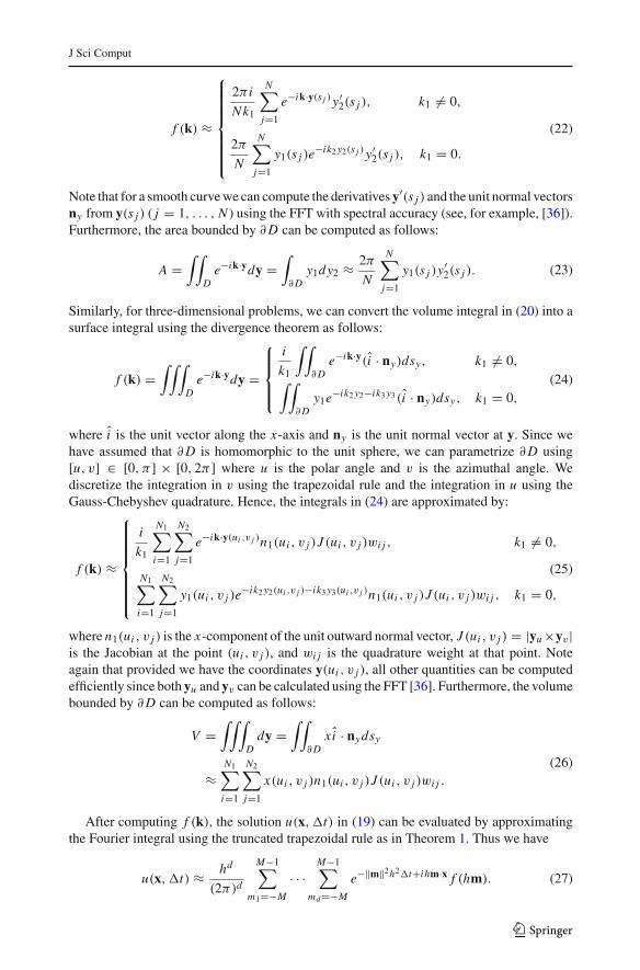
Fig. 6 Snapshots of the volume preserving motion of a wedge. �t = 0.001
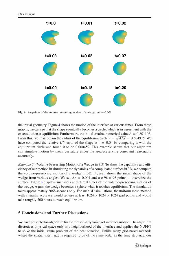
the initial geometry. Figure4 shows the motion of the interface at various times. From thesegraphs, we can see that the shape eventually becomes a circle, which is in agreement with theexact solution at equilibrium.Furthermore, the initial area has numerical value A = 0.801106.From this, we may obtain the radius of the equilibrium circle r = √
A/π = 0.504975. Wehave computed the relative L∞ error of the shape at t = 0.04 by comparing it with theequilibrium circle and found it to be 0.000459. This example shows that our algorithmcan simulate motion by mean curvature under the area-preserving constraint reasonablyaccurately.
Example 5 (Volume-Preserving Motion of a Wedge in 3D) To show the capability and effi-ciency of our method in simulating the dynamics of a complicated surface in 3D, we computethe volume-preserving motion of a wedge in 3D. Figure5 shows the initial shape of thewedge from various angles. We set �t = 0.001 and use 96 × 96 points to discretize thesurface. Figure6 displays snapshots at different times of the volume-preserving motion ofthe wedge. Again, the wedge becomes a sphere when it reaches equilibrium. The simulationtakes approximately 2068 seconds only. For such 3D simulations, the uniform mesh methodwith a similar accuracy would require at least 1024 × 1024 × 1024 grid points and wouldtake roughly 200 hours to reach equilibrium.
5 Conclusions and Further Discussions
Wehave presented an algorithm for the threshold dynamics of interfacemotion. The algorithmdiscretizes physical space only in a neighborhood of the interface and applies the NUFFTto solve the initial value problem of the heat equation. Unlike many grid-based methodswhere the spatial mesh size is required to be of the same order as the time step size, our
123

J Sci Comput
numerical experiments show that the spatial mesh size can be chosen based upon the accuracyconsideration only and thus ismore or less independent of the time step size for our algorithm.Hence, our algorithm is efficient and robust for smooth interfaces if the time step is nottoo small. When the time step is very small, the number of Fourier modes in the spectralapproximation of the heat kernel becomes excessively large and the accuracy of our algorithmdecreases, especially for three-dimensional problems. However, other fast algorithms suchas the fast Gauss transform or even asymptotic analysis can be used to obtain the solution tothe heat equation for the diffusion stage in this regime.
For two-dimensional problems, our algorithm can be easily extended to treat piecewisesmooth boundaries such as polygons, or multiphase flows such as wetting problems on a solidsurface with a given contact angle. For three-dimensional problems, it is straightforward tomodify our algorithm to handle the wetting problems on a flat solid plane. Our algorithm canalso be extended to treat cases involving topological changes. We are currently working onthese extensions.
Acknowledgements S. Jiang was supported by the National Science Foundation under Grant DMS-1418918.X. P. Wang was supported in part by the Hong Kong RGC-GRF Grants 605513 and 16302715, RGC-CRFGrant C6004-14G, and NSFC-RGC joint research Grant N-HKUST620/15.
References
1. Barles, G., Georgelin, C.: A simple proof of convergence for an approximation scheme for computingmotions by mean curvature. SIAM J. Numer. Anal. 32(2), 484–500 (1995)
2. Chambolle, A., Novaga, M.: Convergence of an algorithm for the anisotropic and crystalline mean cur-vature flow. SIAM J. Math. Anal. 37(6), 1978–1987 (2006)
3. Deckelnick, K., Dziuk, G., Elliott, C.M.: Computation of geometric partial differential equations andmean curvature flow. Acta Numerica 14, 139–232 (2005)
4. Dutt, A., Rokhlin, V.: Fast Fourier transforms for nonequispaced data. SIAM J. Sci. Comput. 14, 1368–1393 (1993)
5. Dutt, A., Rokhlin, V.: Fast Fourier transforms for nonequispaced data. II. Appl. Comput. Harmon. Anal.2, 85–100 (1995)
6. Dym, H., McKean, H.P.: Fourier Series and Integrals. Academic Press, Cambridge (1972)7. Esedoglu, S., Otto, F.: Threshold dynamics for networks with arbitrary surface tensions. Comm. Pure
Appl. Math. 68, 808–864 (2015)8. Esedoglu, S., Ruuth, S., Tsai, R.: Threshold dynamics for high order geometric motions. Interf. Free
Bound. 10(3), 263–282 (2008)9. Esodoglu, S., Smereka, P.: A variational formulation for a level set representation of multiphase flow and
area preserving curvature flow. Comm. Math. Sci. 6(1), 125–148 (2008)10. Evans, L.C.: Convergence of an algorithm for mean curvature motion. Indiana Math. J. 42(2), 533–557
(1993)11. Evans, L.C.: Partial Differential Equations, 2nd edn. American Mathematical Society, Providence (2010)12. Gao, M., Wang, X.: A gradient stable scheme for a phase field model for the moving contact line problem.
J. Comput. Phys. 231, 1372–386 (2012)13. Greengard, L., Lee, J.Y.: Accelerating the nonuniform fast Fourier transform. SIAMRev. 46(3), 443–454
(2004)14. Greengard, L., Lin, P.: Spectral approximation of the free-space heat kernel. Appl. Comput. Harmon.
Anal. 9(1), 83–97 (2000)15. Greengard, L., Strain, J.: The fast Gauss transform. SIAM J. Sci. Statist. Comput. 12(1), 79–94 (1991)16. Greengard, L., Sun, X.: A new version of the fast Gauss transform. Proc. Int. Cong. Math. III, 575–584
(1998)17. Ilmanen, T.: Lectures on Mean Curvature Flow and Related Equations, Lecture Notes. ICTP, Trieste
(1995). http://www.math.ethz.ch/~ilmanen/papers/pub.html18. Ishii, K.: Optimal rate of convergence of the Bence–Merriman–Osher algorithm for motion by mean
curvature. SIAM J. Math. Anal. 37(3), 841–866 (2005)
123

J Sci Comput
19. Kublik, C., Esedoglu, S., Fessler, J.A.: Algorithms for area preserving flows. SIAM J. Sci. Comput. 33(5),2382–2401 (2011)
20. Lee, J.Y., Greengard, L., Gimbutas, Z.: NUFFT Version 1.3.2 Software Release. http://www.cims.nyu.edu/cmcl/nufft/nufft.html (2009)
21. Leung, S., Zhao, H.: A grid based particle method for moving interface problems. J. Comput. Phys.228(8), 2993–3024 (2009)
22. Li, J.R., Greengard, L.: On the numerical solution of the heat equation. I. Fast solvers in free space. J.Comput. Phys. 226(2), 1891–1901 (2007)
23. Mascarenhas, P.:DiffusionGeneratedMotionbyMeanCurvature.Department ofMathematics.Universityof California, Los Angeles, Los Angeles (1992)
24. Merriman, B., Bence, J.K., Osher, S.: Diffusion generatedmotion bymean curvature. UCLACAMReport92-18 (1992)
25. Müller, D.E.: A method for solving algebraic equations using an automatic computer. Math. Tables AidsComput. 10, 208–215 (1956)
26. Mullins, W.W.: Two-dimensional motion of idealized grain boundaries. J. Appl. Phys. 27(8), 900–904(1956)
27. Osher, S., Sethian, J.: Fronts propagatingwith curvature-dependent speed: algorithms based onHamilton–Jacobi formulations. J. Comput. Phys. 79(1), 12–49 (1988)
28. Randol, B.: On the Fourier transform of the indicator function of a planar set. Trans. Amer. Math. Soc.139, 271–278 (1969)
29. Ruuth, S.: An algorithm for generating motion by mean curvature. ICAOS’96 pp. 82–91 (1996)30. Ruuth, S.J.: Efficient algorithms for diffusion-generated motion by mean curvature. Ph.D. thesis, Univer-
sity of British Columbia, Vancouver, Canada (1996)31. Ruuth, S.J.: A diffusion-generated approach to multiphase motion. J. Comput. Phys. 145(1), 166–192
(1998)32. Ruuth, S.J.: Efficient algorithms for diffusion-generated motion by mean curvature. J. Comput. Phys.
144(2), 603–625 (1998)33. Ruuth, S.J., Wetton, B.T.: A simple scheme for volume-preserving motion by mean curvature. J. Sci.
Comput. 19(1–3), 373–384 (2003)34. Stenger, F.: Numericalmethods based onWhittaker cardinal, or sinc functions. SIAMRev. 23(2), 165–224
(1981)35. Svadlenka, K., Ginder, E., Omata, S.: A variational method for multiphase volume-preserving interface
motions. J. Comput. Appl. Math. 257, 157–179 (2014)36. Trefethen, L.N.: Spectral Methods in MATLAB. SIAM, Philadelphia (2000)37. Womble, D.E.: A front-tracking method for multiphase free boundary problems. SIAM J. Numer. Anal.
26(2), 380–396 (1989)38. Xu, X., Wang, D., Wang, X.P.: An efficient threshold dynamics method for wetting on rough surfaces. J.
Comput. Phys. 330, 510–528 (2017)39. Yue, P., Feng, J., Liu, C., Shen, J.: A diffuse-interface method for simulating two-phase flows of complex
fluids. J. Fluid Mech. 515, 293–317 (2004)40. Zhao, H., Chan, T., Merriman, B., Osher, S.J.: A variational level set approach to multiphase motion. J.
Comput. Phys. 127(1), 179–195 (1996)
123