Boundary Integral Equations in Linearly Graded Media

Brad Nelson

Senior ThesisDepartment of Mathematics

Dartmouth College

Advisor: Alex Barnett

May 28, 2013

1

Abstract

Boundary integral equations (BIEs) are a popular method for numerical solutionof Helmholtz boundary value problems in a piecewise-uniform medium. We generalizeBIEs for the first time to a continuously-graded medium in two dimensions, where thesquare of the wavenumber varies linearly with one coordinate. Using these techniques,we gain a significant advantage over the alternative finite element/finite differenceschemes for solving scattering problems in this type of medium. Applications includeacoustics and optics with thermal/density/index gradient. We present an evaluationscheme for the fundamental solution using contour integrals, and give examples ofinterior/exterior Dirichlet problems, as well as high-frequency scattering problems.

2

Acknowledgements

First and foremost, I would like to thank Professor Barnett for his mentorship andassistance throughout this project, as well as his guidance in my attempts to navigatethe world of mathematics.

A portion of this research was completed during Spring term 2012, and was madepossible through a grant from the Paul K. Richter and Evalyn E. Cook Richter Memo-rial Fund.

I would also like to thank the Neukom Institute at Dartmouth College for providinga travel grant to present a version of this work at the SIAM CSE 2013 conference in astudent poster session.

3

1 Introduction

Boundary value problems (BVPs) arise when modeling many kinds of natural phe-nomena, including electromagnetics, acoustics, and optics. A BVP seeks a functionthat satisfies a partial differential equation (PDE) within a domain, and that satisfiesboundary conditions along the boundary of the domain. If we let L be a second-orderpartial-differential operator, we formulate a boundary value problem for a function uas

Lu = 0 in Ω

u = f on ∂Ω(1)

where Ω is an interior or exterior domain, ∂Ω denotes its boundary, and f is a givenfunction f : ∂Ω → R. Boundary data that requires u = f , as above, is known asDirichlet boundary data. Boundary data that matches the normals derivative of uto a function, un = f , is known as Neumann boundary data. Mixed boundary datarequires u + βun = f for some β ∈ C. In interior problems, Ω is a simply-connected,bounded domain. In exterior problems, including scattering problems, the domain’scomplement is simply-connected and bounded. In this thesis, we primarily considerboth interior and exterior problems with Dirichlet boundary data.

Two common examples of boundary value problems are the Laplace and Helmholtzproblems. Both equations are useful in describing electromagnetic, acoustic, and opticalphenomena. A Helmholtz BVP, which describes a wave function u, is formulated as

(∆ + k2(x))u = 0 in Ω

u = f on ∂Ω(2)

where x = (x1, x2, . . . ), k(x) is the location-dependent wavenumber of u, and ∆ is theLaplacian operator,

∆ =∑i

∂2

∂x2i

(3)

The Laplace equation is similar to the Helmholtz, except k2 = 0 everywhere.Classic techniques for solving BVPs numerically are the finite element and finite

difference methods. Both methods involve a discretization of the domain of the prob-lem, and matching conditions at each point. For instance, if we are interested in solvinga BVP in the unit square using the finite difference method, then the system will bediscretized into n × n points, resulting in n2 unknowns. This results in an n2 × n2

linear system that is sparse, but poorly conditioned, demanding complicated precondi-tioners if an iterative solver is used [10]. Additionally, solving exterior problems usingthese methods require artificial conditions, such as perfectly matched layers (PMLs)to handle radiation conditions.

Boundary integral equations (BIEs) are a popular alternative to these classicaldiscretization schemes for Helmholtz and Laplace BVPs in (piecewise) uniform media(meaning that k(x) is piecewise constant in the domain). BIEs reduce the problemto solving a linear system on the boundary of the domain, so the size of the problemgrows with the perimeter of the domain, rather than its volume. Additionally, BIEshave the advantage of being well-conditioned, allowing for accurate solution of thelinear system using standard linear algebraic techniques, and methods such as the fast

4

multipole method (FMM) allow for iterative solution in near-linear time. BIEs alsohave the advantage of being able to solve exterior BVPs without the use of PMLs.

The particular BVP that is investigated in this thesis is a variation of the Helmholtzequation where k2(x) varies linearly in one coordinate of the domain:

(∆ + x2 + E)u = 0 in Ω

u = f on ∂Ω(4)

Because of the linear term x2, we refer to this as the linear Helmholtz equation. Notethat generally, a PDE with a linear dependence of the form k2(x) = a · x + E can betransformed into equation (4) through a change of variables in the domain. This equa-tion describes natural phenomena such as acoustics in a temperature/density gradient(particularly underwater acoustics), optics in a medium with a linearly graded indexof refraction, and electromagnetic waves or a quantum particle in a linear potential.

5

2 Boundary Integral Equations

2.1 Overview

An integral equation is an equation

b(x) =

∫ b

aK(x, y)τ(y) dy

Where b and K are given, and we are trying to solve for the function τ . This is thecontinuous analog of solving a linear system

b = Kτ

for τ . We refer to K(x, y) as the kernel of the integral equation.The basic idea of BIEs are to use a function, called a fundamental solution, that

satisfies the PDE everywhere but a point, called the source of the fundamental solution,as the kernel of an integral equation. This formulation obeys jump relations, whichallow for boundary data to be matched. By weighting fundamental solution witha density function along the boundary of the domain, we satisfy the PDE and theboundary conditions.

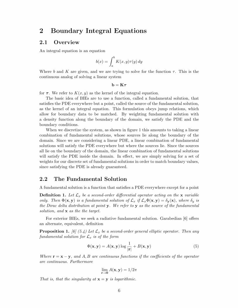
When we discretize the system, as shown in figure 1 this amounts to taking a linearcombination of fundamental solutions, whose sources lie along the boundary of thedomain. Since we are considering a linear PDE, a linear combination of fundamentalsolutions will satisfy the PDE everywhere but where the sources lie. Since the sourcesall lie on the boundary of the domain, the linear combination of fundamental solutionswill satisfy the PDE inside the domain. In effect, we are simply solving for a set ofweights for our discrete set of fundamental solutions in order to match boundary values,since satisfying the PDE is already guaranteed.

2.2 The Fundamental Solution

A fundamental solution is a function that satisfies a PDE everywhere except for a point

Definition 1. Let Lx be a second-order differential operator acting on the x variableonly. Then Φ(x,y) is a fundamental solution of Lx if LxΦ(x,y) = δy(x), where δy isthe Dirac delta distribution at point y. We refer to y as the source of the fundamentalsolution, and x as the the target.

For exterior BIEs, we seek a radiative fundamental solution. Garabedian [6] offersan alternate, equivalent, definition

Proposition 1. [6] (5.4) Let Lx be a second-order general elliptic operator. Then anyfundamental solution for Lx is of the form

Φ(x,y) = A(x,y) log1

|r|+B(x,y) (5)

Where r = x− y, and A,B are continuous functions if the coefficients of the operatorare continuous. Furthermore

limr→0

A(x,y) = 1/2π

That is, that the singularity at x = y is logarithmic.

6

Ω

∂Ω

Figure 1: Example of discretization for an interior boundary value problem usingboundary integral equations. We place fundamental solutions with sources at the reddots, and solve for their weights.

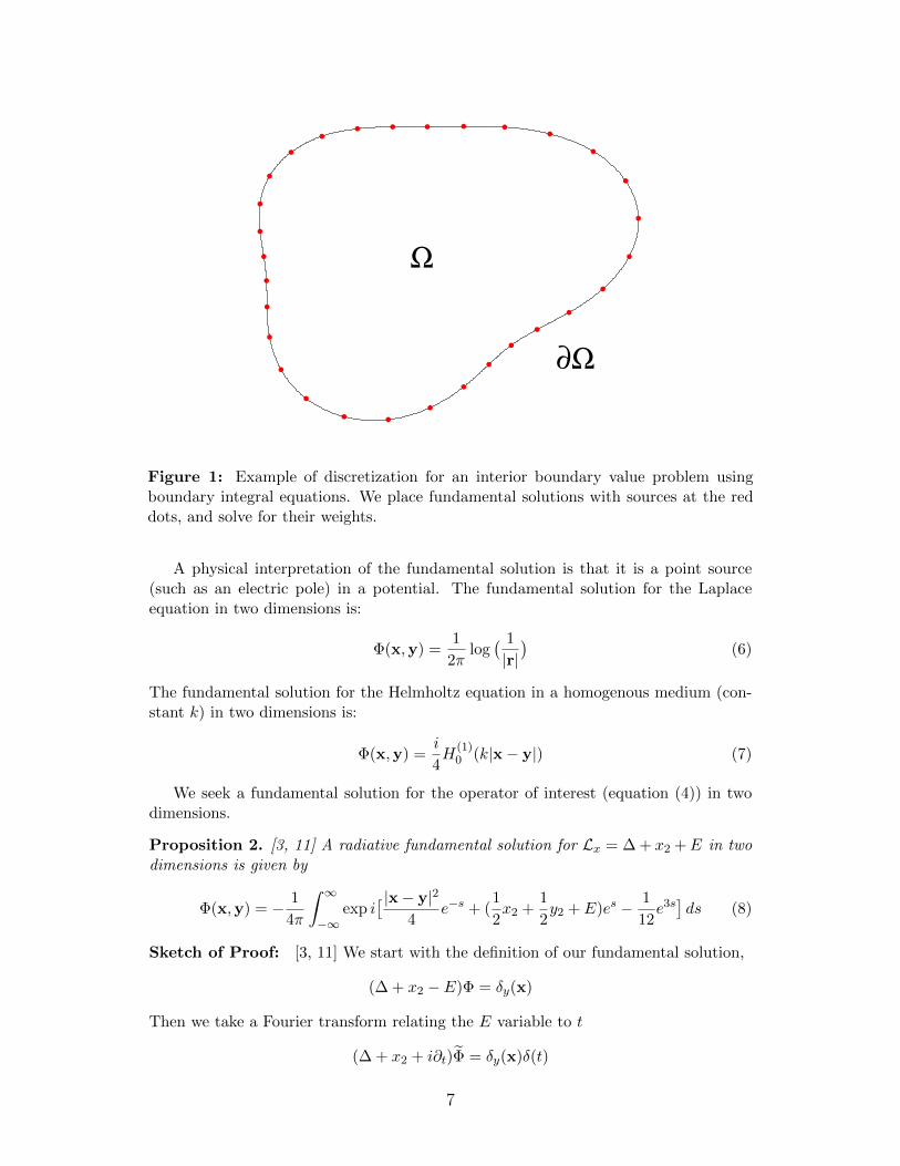
A physical interpretation of the fundamental solution is that it is a point source(such as an electric pole) in a potential. The fundamental solution for the Laplaceequation in two dimensions is:

Φ(x,y) =1

2πlog( 1

|r|)

(6)

The fundamental solution for the Helmholtz equation in a homogenous medium (con-stant k) in two dimensions is:

Φ(x,y) =i

4H

(1)0 (k|x− y|) (7)

We seek a fundamental solution for the operator of interest (equation (4)) in twodimensions.

Proposition 2. [3, 11] A radiative fundamental solution for Lx = ∆ + x2 +E in twodimensions is given by

Φ(x,y) = − 1

4π

∫ ∞−∞

exp i[ |x− y|2

4e−s + (

1

2x2 +

1

2y2 + E)es − 1

12e3s]ds (8)

Sketch of Proof: [3, 11] We start with the definition of our fundamental solution,

(∆ + x2 − E)Φ = δy(x)

Then we take a Fourier transform relating the E variable to t

(∆ + x2 + i∂t)Φ = δy(x)δ(t)

7

−10 −5 0 5 10−10

−8

−6

−4

−2

0

2

4

6

8

10

−10 −5 0 5 10−10

−8

−6

−4

−2

0

2

4

6

8

10

−10 −5 0 5 10−10

−8

−6

−4

−2

0

2

4

6

8

10

Figure 2: Fundamental solutions in the (x1, x2) plane, with y = (0, 0). Top left:fundamental solution for Laplace’s equation (6). Top right: fundamental solution forthe Helmholtz equation (k = 1) (7). Bottom: fundamental solution for the linearHelmholtz equation (E = 1) (8).

This is equivalent to a time-dependent Schrodinger equation in a linear potential, whichcan be solved using yet another Fourier transform in the spatial dimensions, eventuallygiving the above result. This contrasts to the usual frequency-time connection used inthe wave equation.

Since this fundamental solution is derived from the Fourier transform of a causalgreens function for the time-dependent Schrodinger equation, we believe that it is thephysically relevant greens function for the time-harmonic case, meaning that it is anoutwardly radiative solution. However, no formal radiation condition exists in theliterature.

In section 4, we present numerical algorithms to evaluate this fundamental solution.

8

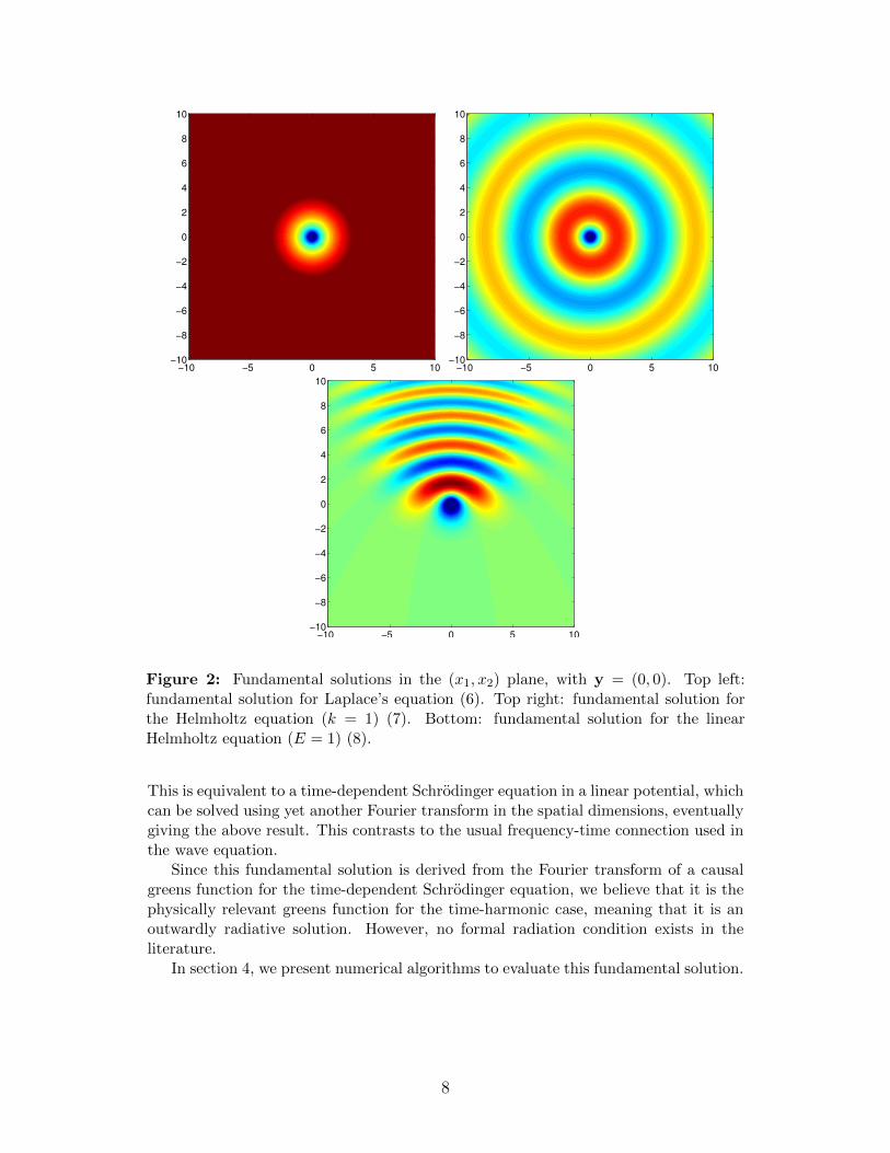
2.2.1 Physical Interpretation

First, we note the connection of our wave equation to the Schrodinger equation, whichdescribes the wave function of a quantum particle. The linear Helmholtz equation:

(∆ + x2 + E)u = 0

becomes[−∆/2 + (−x2/2− E/2)]u = 0

when divided by −2. This is the (dimensionless) time-independent Schrodinger equa-tion

Hu = [−∆/2 + V (x)]u(x) = 0

With potential energy V (x) = −x2/2− E/2.The fundamental solution is thus the solution to the Schrodinger equation with a

point-source at y. This corresponds to the interference pattern of particles emanatingfrom the source in all directions. In order to simulate this, we can start particles atthe source with kinetic energy E/2, and subject them to a force of strength 1/2 in the+x2 direction.

As seen in fig. 3, the fundamental solution dies off in areas where the particles are“classically forbidden,” and follows the parabolic shape of the classical trajectories.

−20 −10 0 10 20−20

−15

−10

−5

0

5

10

15

20

−0.15

−0.1

−0.05

0

0.05

0.1

0.15

Figure 3: Trajectories of classical particles emanating from the origin, E = 5, super-imposed on the fundamental solution for the same E.

2.3 Jump Relations

As mentioned previously, one of the reasons that the fundamental solution is usefulis that it obeys certain relations at the source that allow for matching of boundaryconditions.

9

Definition 2. Given a fundamental solution Φ(x,y) and a domain Ω we define thefollowing integral operators:

(Sσ)(x) =

∫∂Ω

Φ(x,y)σ(y) dy (9)

(Dτ)(x) =

∫∂Ω

∂Φ(x,y)

∂n(y)τ(y) dy (10)

We refer to S as the“single layer representation” and we refer to D as the“double layerrepresentation.” We define the boundary integral operators

(Sσ)(x) = (Sσ)(x), x ∈ ∂Ω (11)

As the restriction of (Sσ) to ∂Ω, and

(Dτ)(x) (12)

principle value integral of (10) with x on the boundary ∂Ω. We refer to these twoboundary integral operators as the “single layer operator” and “double layer operator”respectively.

Theorem 1. Let ∂Ω be of class C2, density σ be continuous. Define

u(x) = (Sσ)(x) (13)

then u(x) is uniformly continuous in R2.

Theorem 2. Let ∂Ω be of class C2, density τ be continuous. Define

v(x) = (Dτ)(x) x ∈ R2 − ∂Ω (14)

Thenv±(x) = (Dτ)(x)± τ(x)/2 x ∈ ∂Ω (15)

wherev±(x) = lim

h→0+v(x± hn(x))

For proof of Theorems 1 and 2 for the Laplace and homogeneous Helmholtz equa-tions, we refer to [4].

To sketch a proof for the linear Helmholtz case, we note that Proposition 1 givesus that the fundamental solution (8) is a continuous perturbation of the fundamentalsolution of the Laplace equation (6), and has an identical singularity at the source.Following the proof of the jump relations in Garabedian [6] 5.1, we form a contourencircling the source of an isolated fundamental solution. Since the fundamental so-lution locally resembles the fundamental solution for Laplace’s equation, as we shrinkthe radius of the contour, the integral over the contour for both fundamental solutionsagree. Since the evaluation of this integral gives the jump relations, we see that thejump relations hold for the linear Helmholtz fundamental solution.

10

2.4 Integral Equations

Now, since we seek a solution to a Dirichlet BVP (1), we see that the jump relationsgive us an easy solution. We simply need to find a single layer density σ(x) or doublelayer density τ(x) such that Sσ or (D ± 1/2)τ agrees with the given boundary data.The single-layer operator gives a Fredholm integral equation of the first kind, whichis subject to ill-conditioning, making it difficult to solve accurately. But, the doublelayer operator gives a Fredholm integral equation of the second kind, which is well-conditioned, so we will focus on this formulation of the problem.

For an interior Dirichlet Problem, it suffices to use the double layer operator. How-ever, exterior/scattering problems are subject to spurious resonances. To avoid thisproblem, we use the kernel

D − iηS (16)

which also provides a second-kind formulation:

(1/2 +D − iηS)τ = f (17)

We call this the combined field integral equation [5]. Generally, we take η ≈ k for thehomogenous Helmholtz equation. Since the wavenumber varies over the domain in thelinear Helmholtz case, we will take η =

√E.

11

3 Nystrom Method & Quadrature

In the previous section, we outlined the formulation of a boundary integral equation.However, to solve such problems numerically, we must discretize the boundary of thedomain, and use quadrature rules to evaluate the integral. This section contains adiscussion of the discretization of the integral and a discussion of dealing with thesingular operator.

In this section we consider the general smooth integral operator

(Kτ)(x) =

∫∂ΩK(x,y)τ(y) dy (18)

where we are integrating over the length of the boundary.

3.1 Nystrom Method

In order to evaluate our integral operators numerically, we rely on the Nystrom methodof approximating the integral. This method discretizes the domain of the integral, andtakes a weighted sum of the integrand at each point in the discretization.∫ b

ah(t) dt ≈

N∑i=1

wih(ti) (19)

Using the Nystrom method, our integral operator (18) becomes

(Kτ)(x) ≈N∑i=1

wiK(x,yi)τ(yi) (20)

where yini=1 lies on the boundary. Kress [9] describes in detail how the above dis-cretization yield a convergent approximation as N is increased.

3.1.1 Periodic Trapezoid Rule

Now, consider BVPs where the domain has a smooth boundary. Let y(t) be a 2π peri-odic parameterization of this boundary. We can recast our boundary integral equationin terms of this parameterization as∫

∂ΩK(x,y)τ(y) dy =

∫ 2π

0K(x,y(t))τ(y(t))

d|y|dt

dt (21)

Since the function y(t) is periodic over 2π, we can use the periodic trapezoid rule as aquadrature rule. That is if we discretize the domain of the integral into N points, weuse

tk = 2πkN

wk = 2πN

(22)

This quadrature rule is exponentially convergent for analytic functions ([9] 12.1). Thusthe Nystrom method is exponentially convergent if K is analytic in both variables.Using these nodes and weights, equation (19) becomes∫ b

ah(t) dt ≈

N∑i=1

2π

Nh(2πi

N

)12

Now, we note that if we are trying to match conditions on the boundary, i.e. weare solving for τ in the equation

Kτ = f |∂Ω

where f is gives the boundary data. Then we just need to solve the linear system

f(y(ti)) =

n∑k=1

wkK(y(ti),y(tk))d|y|dt

(tk)τ(y(tk)) ∀i = 0 to n (23)

Which we will denotef = Aτ (24)

where

Ai,j = wjK(y(ti),y(tj))d|y(tj)|dt

(25)

is an N ×N matrix, and fi = f(y(ti)) and τ i = τ(y(ti)) are N × 1 vectors. τ is ourunknown density function, as in (17)

Now, solving for τ is a standard linear algebra problem. We can use τ in equation(20) to approximate the desired function (Kτ)(x).

(Kτ)(x) ≈N∑i=1

wiK(x,y(ti))d|y|dt

(ti)τ i (26)

3.2 Alpert Corrections

In the preceding sections, we have introduced the Nystrom method of solving integralequations for a general smooth kernel K. Now, we wish to focus on the kernel Φ(x,y)given by equation (8) which has a logarithmic singularity at the source x = y.

From equation (1) we have that Φ(x,y) = A(x,y) log 1r +B(x,y). The main prob-

lem that we face using periodic trapezoid rule is that we must evaluate the fundamentalsolution at the singularity in order to fill the Nystrom matrix A along the diagonalwhere y(ti) = y(tj). In order to obtain a high-order convergent scheme for evaluatingintegral equations with a logarithmic singularity, we use Alpert corrections [1, 7].

If we have an underlying N + 1 node periodic trapezoid rule scheme, Alpert cor-rections will leave N − 2a + 1 nodes unaltered with the same weights. The a nodesto either side of the singularity are replaced with m nodes each, with positions andweights chosen using barycentric interpolation ([1] section 5 describes how to calculatethese nodes and weights). These nodes will lie off the underlying periodic-trapezoidgrid, with several nodes clustered near, but not lying on the singularity. We are thenable to solve the system on these new nodes, and interpolate τ measured at theseAlpert nodes to τ using the original periodic trapezoid nodes.

This scheme has been proven to have O(hl log(h)) error convergence as h → 0 ([1]Cor. 3.8) for functions of form (1), where h = 2π/N . The number of new nodes m oneither side of the singularity is either l or l − 1 [7].

From [7], we see that choosing a = 10,m = 15 gives l = 16, which are the values thatwe used in our implementation. Note that this requires that N > 2m. We make thesecorrections on each row of the matrix, since we must integrate over each fundamentalsolution. Since we only need make O(1) corrections per source, the total number ofcorrections made to our matrix A (eqn. (24)) is O(N).

13

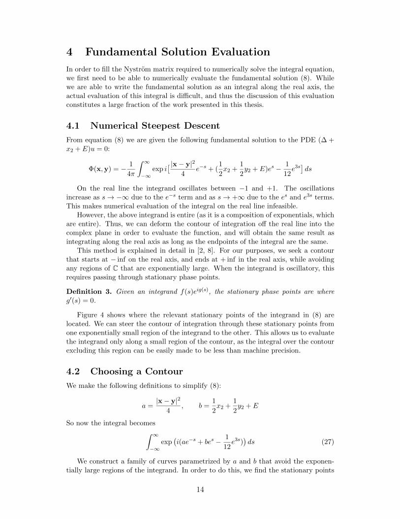
4 Fundamental Solution Evaluation

In order to fill the Nystrom matrix required to numerically solve the integral equation,we first need to be able to numerically evaluate the fundamental solution (8). Whilewe are able to write the fundamental solution as an integral along the real axis, theactual evaluation of this integral is difficult, and thus the discussion of this evaluationconstitutes a large fraction of the work presented in this thesis.

4.1 Numerical Steepest Descent

From equation (8) we are given the following fundamental solution to the PDE (∆ +x2 + E)u = 0:

Φ(x,y) = − 1

4π

∫ ∞−∞

exp i[ |x− y|2

4e−s + (

1

2x2 +

1

2y2 + E)es − 1

12e3s]ds

On the real line the integrand oscillates between −1 and +1. The oscillationsincrease as s→ −∞ due to the e−s term and as s→ +∞ due to the es and e3s terms.This makes numerical evaluation of the integral on the real line infeasible.

However, the above integrand is entire (as it is a composition of exponentials, whichare entire). Thus, we can deform the contour of integration off the real line into thecomplex plane in order to evaluate the function, and will obtain the same result asintegrating along the real axis as long as the endpoints of the integral are the same.

This method is explained in detail in [2, 8]. For our purposes, we seek a contourthat starts at − inf on the real axis, and ends at + inf in the real axis, while avoidingany regions of C that are exponentially large. When the integrand is oscillatory, thisrequires passing through stationary phase points.

Definition 3. Given an integrand f(s)eig(s), the stationary phase points are whereg′(s) = 0.

Figure 4 shows where the relevant stationary points of the integrand in (8) arelocated. We can steer the contour of integration through these stationary points fromone exponentially small region of the integrand to the other. This allows us to evaluatethe integrand only along a small region of the contour, as the integral over the contourexcluding this region can be easily made to be less than machine precision.

4.2 Choosing a Contour

We make the following definitions to simplify (8):

a =|x− y|2

4, b =

1

2x2 +

1

2y2 + E

So now the integral becomes∫ ∞−∞

exp(i(ae−s + bes − 1

12e3s)

)ds (27)

We construct a family of curves parametrized by a and b that avoid the exponen-tially large regions of the integrand. In order to do this, we find the stationary points

14

Re(s)

Im(s

)

−5 0 5−5

−4

−3

−2

−1

0

1

2

3

4

5

Figure 4: Integrand for a = b = 4. Stationary points are marked with x

for the integrand, which are centered in the calm regions of the integrand and serve asthe gateways from one exponentially small region to another.

We find the stationary points for (27) as follows [11]

d

ds[ae−s + bes − 1

12e3s] = 0 Definition 3

−ae−s + bes − 1

4e3s = 0

1

4e4s + be2s − a = 0 multiplication by es

e2s = 2(b±√b2 − a) quadratic formula

es = ±√

2(b±√b2 − a)

s = log±√

2(b±√b2 − a)

Thus, for any branch of log, there are four stationary points:

σstat = log±√

2(b±√b2 − a)

For concreteness, let σ1 = log√

2(b+√b2 − a) and σ2 = log

√2(b−

√b2 − a).

A family of contours that steers through these stationary points into exponentiallysmall regions of the integrand is given by [11] and written as:

γ(t) = t+ iga,b(t),

15

where

ga,b(t) =

13 arctan(x)− π

3 : b ≤√a, Im(σ2) ≤ −π/3

(Im(σ2) + π3 ) exp (−(t− Re(σ2))2) + 1

3 arctan(x)− π3 : b ≤

√a, Im(σ2) ≥ −π/3(

( 1π + 1

2) arctan(2(t− Re(σ2) + w2 ))− (π4 −

12))×(

( 1π + 1

6) arctan(−4(t− Re(σ1)− v4 ))− ( π12 −

12))

: otherwise

where in the last line v = tan(π2−6π

12+2π ) and w = tan(π2−2π

4+2π ).

These formulas are messy, but basic idea is to perturb the contour below the realaxis, so the contour lies in exponentially small regions of the s-plane as it goes to ±∞,and steer through the stationary points with a bump shaped function. In figure 4, wesee that there are multiple regions in which the integrand dies off as s→ ±∞. Thesecorrespond to different branch cuts of the integrand. Steering through the two regionsdirectly below the real axis give us the desired result.

Note on Stationary Point Evaluation:We wish for σ2 to be continuous over the a, b plane. If we transition from a regionwhere b2 − a is positive to a region where it is negative, the expression b −

√b2 − a

moves from the real line into the bottom-half of the complex plane. We have that

σ2 = log(

√2(b−

√b2 − a)) =

1

2log(2(b−

√b2 − a))

Since the quantity evaluated by the logarithm lies in the upper complex plane in theleft-hand expression, and the lower-complex plane in the right hand expression, if thebranch cut of the logarithm lies along the negative real axis (as is standard), the leftand right hand expressions will disagree by iπ. To ensure that σ2 steers the contourinto the correct region, we found that it was necessary to enforce Im(σ2) < 0

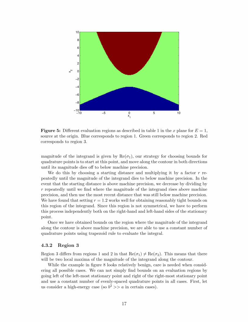
4.3 Evaluation in Different Regions

So far, we have chosen contours that steer into exponentially decaying regions of theintegrand. Now, we consider evaluation depending on the form of the contour. We usethe following shorthand to differentiate regions where the contour is chosen differently:

Region Description

1 b ≤√a, Im(σ2) ≤ −π/3

2 b ≤√a, Im(σ2) ≥ −π/3

3 b >√a

Table 1: evaluation regions of integrand

4.3.1 Regions 1 & 2

Regions 1 and 2 are both similar in that Re(σ1) = Re(σ2) So there in only one maximumin the magnitude of the integrand when following the contour. Since the maximum

16

x1

x2

−10 −5 0 5 10−10

−8

−6

−4

−2

0

2

4

6

8

10

Figure 5: Different evaluation regions as described in table 1 in the x plane for E = 1,source at the origin. Blue corresponds to region 1. Green corresponds to region 2. Redcorresponds to region 3.

magnitude of the integrand is given by Re(σ1), our strategy for choosing bounds forquadrature points is to start at this point, and move along the contour in both directionsuntil its magnitude dies off to below machine precision.

We do this by choosing a starting distance and multiplying it by a factor r re-peatedly until the magnitude of the integrand dies to below machine precision. In theevent that the starting distance is above machine precision, we decrease by dividing byr repeatedly until we find where the magnitude of the integrand rises above machineprecision, and then use the most recent distance that was still below machine precision.We have found that setting r = 1.2 works well for obtaining reasonably tight bounds onthis region of the integrand. Since this region is not symmetrical, we have to performthis process independently both on the right-hand and left-hand sides of the stationarypoint.

Once we have obtained bounds on the region where the magnitude of the integrandalong the contour is above machine precision, we are able to use a constant number ofquadrature points using trapezoid rule to evaluate the integral.

4.3.2 Region 3

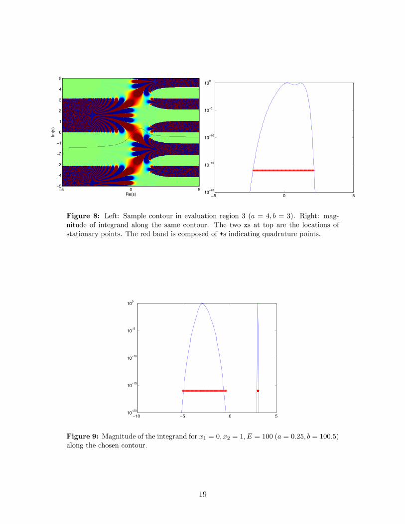
Region 3 differs from regions 1 and 2 in that Re(σ1) 6= Re(σ2). This means that therewill be two local maxima of the magnitude of the integrand along the contour.

While the example in figure 8 looks relatively benign, care is needed when consid-ering all possible cases. We can not simply find bounds on an evaluation regions bygoing left of the left-most stationary point and right of the right-most stationary pointand use a constant number of evenly-spaced quadrature points in all cases. First, letus consider a high-energy case (so b2 >> a in certain cases).

17

Re(s)

Im(s

)

−5 0 5−5

−4

−3

−2

−1

0

1

2

3

4

5

Re(s)

Im(s

)

−5 0 5−5

−4

−3

−2

−1

0

1

2

3

4

5

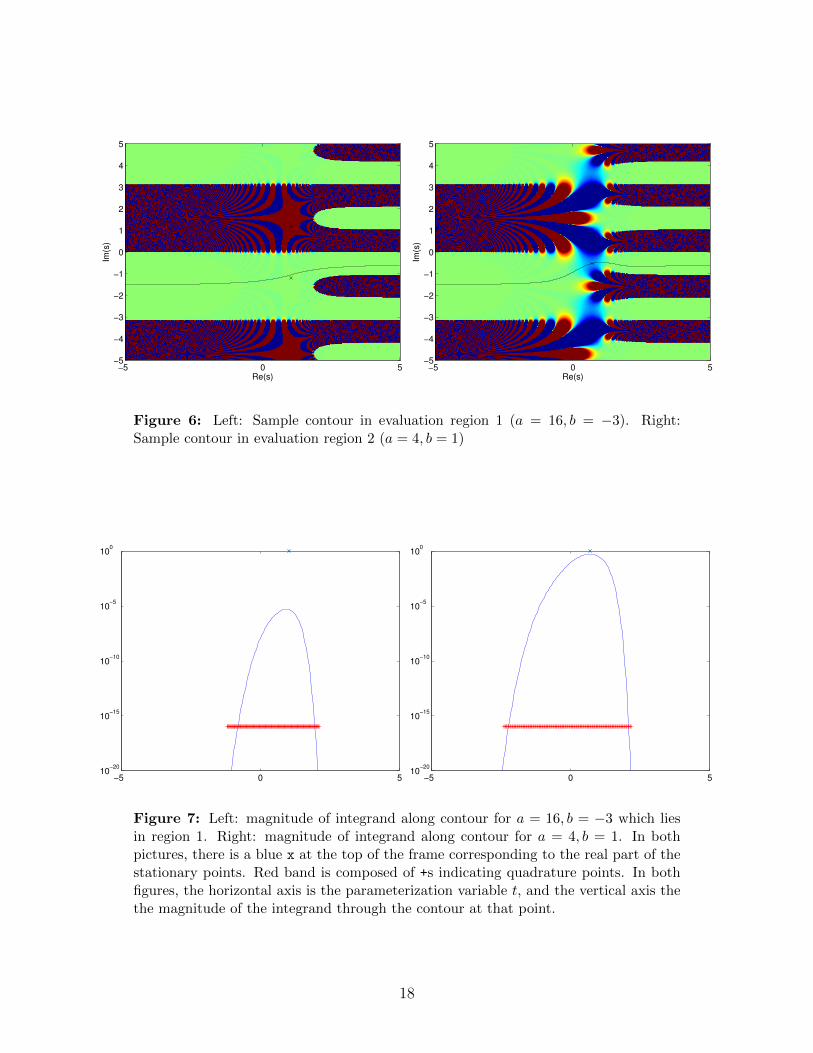
Figure 6: Left: Sample contour in evaluation region 1 (a = 16, b = −3). Right:Sample contour in evaluation region 2 (a = 4, b = 1)

−5 0 510

−20

10−15

10−10

10−5

100

−5 0 510

−20

10−15

10−10

10−5

100

Figure 7: Left: magnitude of integrand along contour for a = 16, b = −3 which liesin region 1. Right: magnitude of integrand along contour for a = 4, b = 1. In bothpictures, there is a blue x at the top of the frame corresponding to the real part of thestationary points. Red band is composed of +s indicating quadrature points. In bothfigures, the horizontal axis is the parameterization variable t, and the vertical axis thethe magnitude of the integrand through the contour at that point.

18

Re(s)

Im(s

)

−5 0 5−5

−4

−3

−2

−1

0

1

2

3

4

5

−5 0 510

−20

10−15

10−10

10−5

100

Figure 8: Left: Sample contour in evaluation region 3 (a = 4, b = 3). Right: mag-nitude of integrand along the same contour. The two xs at top are the locations ofstationary points. The red band is composed of +s indicating quadrature points.

−10 −5 0 510

−20

10−15

10−10

10−5

100

Figure 9: Magnitude of the integrand for x1 = 0, x2 = 1, E = 100 (a = 0.25, b = 100.5)along the chosen contour.

19

10−6

10−4

10−2

100

102

0

5

10

15

20

25

30

35

|x−y|

length

of in

terv

al

−25 −20 −15 −10 −5 0 510

−20

10−15

10−10

10−5

100

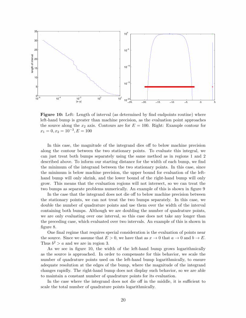
Figure 10: Left: Length of interval (as determined by find endpoints routine) whereleft-hand bump is greater than machine precision, as the evaluation point approachesthe source along the x2 axis. Contours are for E = 100. Right: Example contour forx1 = 0, x2 = 10−3, E = 100

In this case, the magnitude of the integrand dies off to below machine precisionalong the contour between the two stationary points. To evaluate this integral, wecan just treat both bumps separately using the same method as in regions 1 and 2described above. To inform our starting distance for the width of each bump, we findthe minimum of the integrand between the two stationary points. In this case, sincethe minimum is below machine precision, the upper bound for evaluation of the left-hand bump will only shrink, and the lower bound of the right-hand bump will onlygrow. This means that the evaluation regions will not intersect, so we can treat thetwo bumps as separate problems numerically. An example of this is shown in figure 9

In the case that the integrand does not die off to below machine precision betweenthe stationary points, we can not treat the two bumps separately. In this case, wedouble the number of quadrature points and use them over the width of the intervalcontaining both bumps. Although we are doubling the number of quadrature points,we are only evaluating over one interval, so this case does not take any longer thanthe preceding case, which evaluated over two intervals. An example of this is shown infigure 8.

One final regime that requires special consideration is the evaluation of points nearthe source. Since we assume that E > 0, we have that as x→ 0 that a→ 0 and b→ E.Thus b2 > a and we are in region 3.

As we see in figure 10, the width of the left-hand bump grows logarithmicallyas the source is approached. In order to compensate for this behavior, we scale thenumber of quadrature points used on the left-hand bump logarithmically, to ensureadequate resolution at the edges of the bump, where the magnitude of the integrandchanges rapidly. The right-hand bump does not display such behavior, so we are ableto maintain a constant number of quadrature points for its evaluation.

In the case where the integrand does not die off in the middle, it is sufficient toscale the total number of quadrature points logarithmically.

20

0 50 100 150 20010

−15

10−10

10−5

100

num quad pts

err

or

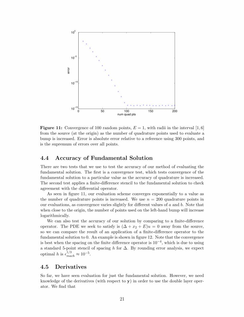
Figure 11: Convergence of 100 random points, E = 1, with radii in the interval [1, 6]from the source (at the origin) as the number of quadrature points used to evaluate abump is increased. Error is absolute error relative to a reference using 300 points, andis the supremum of errors over all points.

4.4 Accuracy of Fundamental Solution

There are two tests that we use to test the accuracy of our method of evaluating thefundamental solution. The first is a convergence test, which tests convergence of thefundamental solution to a particular value as the accuracy of quadrature is increased.The second test applies a finite-difference stencil to the fundamental solution to checkagreement with the differential operator.

As seen in figure 11, our evaluation scheme converges exponentially to a value asthe number of quadrature points is increased. We use n = 200 quadrature points inour evaluations, as convergence varies slightly for different values of a and b. Note thatwhen close to the origin, the number of points used on the left-hand bump will increaselogarithmically.

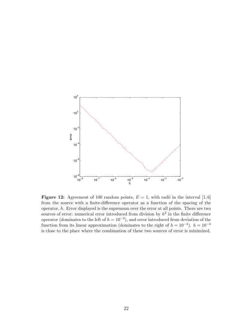
We can also test the accuracy of our solution by comparing to a finite-differenceoperator. The PDE we seek to satisfy is (∆ + x2 + E)u = 0 away from the source,so we can compare the result of an application of a finite-difference operator to thefundamental solution to 0. An example is shown in figure 12. Note that the convergenceis best when the spacing on the finite difference operator is 10−4, which is due to usinga standard 5-point stencil of spacing h for ∆. By rounding error analysis, we expect

optimal h is ε1/3mach ≈ 10−5.

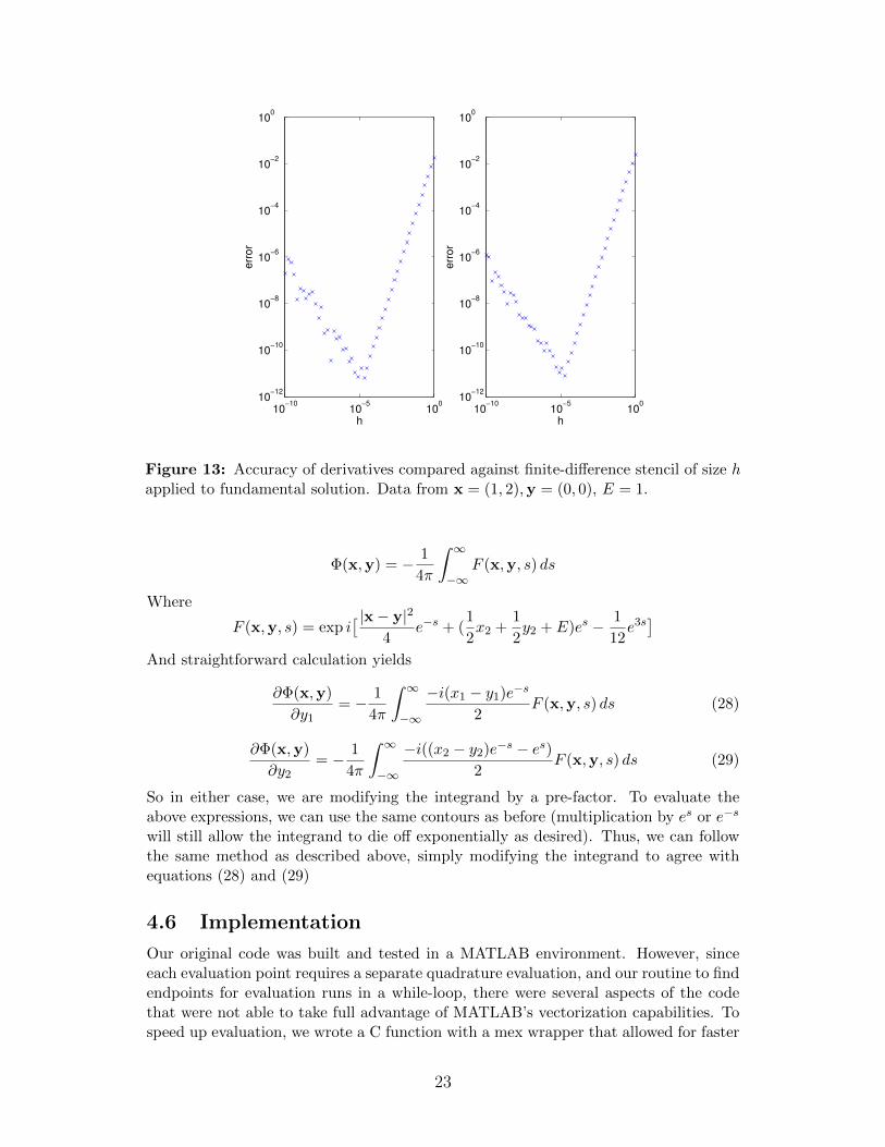
4.5 Derivatives

So far, we have seen evaluation for just the fundamental solution. However, we needknowledge of the derivatives (with respect to y) in order to use the double layer oper-ator. We find that

21

10−8

10−7

10−6

10−5

10−4

10−3

10−2

10−8

10−6

10−4

10−2

100

102

h

err

or

Figure 12: Agreement of 100 random points, E = 1, with radii in the interval [1, 6]from the source with a finite-difference operator as a function of the spacing of theoperator, h. Error displayed is the supremum over the error at all points. There are twosources of error: numerical error introduced from division by h2 in the finite differenceoperator (dominates to the left of h = 10−4), and error introduced from deviation of thefunction from its linear approximation (dominates to the right of h = 10−4). h = 10−4

is close to the place where the combination of these two sources of error is minimized.

22

10−10

10−5

100

10−12

10−10

10−8

10−6

10−4

10−2

100

h

err

or

10−10

10−5

100

10−12

10−10

10−8

10−6

10−4

10−2

100

h

err

or

Figure 13: Accuracy of derivatives compared against finite-difference stencil of size happlied to fundamental solution. Data from x = (1, 2),y = (0, 0), E = 1.

Φ(x,y) = − 1

4π

∫ ∞−∞

F (x,y, s) ds

Where

F (x,y, s) = exp i[ |x− y|2

4e−s + (

1

2x2 +

1

2y2 + E)es − 1

12e3s]

And straightforward calculation yields

∂Φ(x,y)

∂y1= − 1

4π

∫ ∞−∞

−i(x1 − y1)e−s

2F (x,y, s) ds (28)

∂Φ(x,y)

∂y2= − 1

4π

∫ ∞−∞

−i((x2 − y2)e−s − es)2

F (x,y, s) ds (29)

So in either case, we are modifying the integrand by a pre-factor. To evaluate theabove expressions, we can use the same contours as before (multiplication by es or e−s

will still allow the integrand to die off exponentially as desired). Thus, we can followthe same method as described above, simply modifying the integrand to agree withequations (28) and (29)

4.6 Implementation

Our original code was built and tested in a MATLAB environment. However, sinceeach evaluation point requires a separate quadrature evaluation, and our routine to findendpoints for evaluation runs in a while-loop, there were several aspects of the codethat were not able to take full advantage of MATLAB’s vectorization capabilities. Tospeed up evaluation, we wrote a C function with a mex wrapper that allowed for faster

23

10−2

10−1

100

101

102

103

104

103

104

105

106

E

eva

ls/s

ec

Figure 14: Speed of evaluation of the fundamental solution. Each data point wasgenerated by evaluating the fundamental solution at 1000 randomly generated pointsin the annulus of outer radius 10, inner radius 1. Green: MATLAB code. Blue: mexfunction built on C code parallelized to 8 cores of a Xeon 3.3 GHz processor (16 threads).

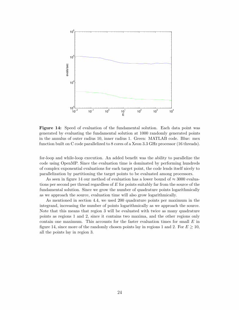
for-loop and while-loop execution. An added benefit was the ability to parallelize thecode using OpenMP. Since the evaluation time is dominated by performing hundredsof complex exponential evaluations for each target point, the code lends itself nicely toparallelization by partitioning the target points to be evaluated among processors.

As seen in figure 14 our method of evaluation has a lower bound of ≈ 3000 evalua-tions per second per thread regardless of E for points suitably far from the source of thefundamental solution. Since we grow the number of quadrature points logarithmicallyas we approach the source, evaluation time will also grow logarithmically.

As mentioned in section 4.4, we used 200 quadrature points per maximum in theintegrand, increasing the number of points logarithmically as we approach the source.Note that this means that region 3 will be evaluated with twice as many quadraturepoints as regions 1 and 2, since it contains two maxima, and the other regions onlycontain one maximum. This accounts for the faster evaluation times for small E infigure 14, since more of the randomly chosen points lay in regions 1 and 2. For E ≥ 10,all the points lay in region 3.

24

5 Results

In this section we explore numerical results of both interior, exterior, and scatteringproblems in two dimensions using the operator in equation (4), with Dirichlet boundarydata. This corresponds to scattering off of a sound-soft obstacle [5].

5.1 Implementation

Numerical experiments were performed in a MATLAB environment.Throughout our experiments, we used boundaries that can be described as a linear

combination of Fourier modes of the circle. That is, if we center the domain at p, wecan parameterize the boundary as having radius

r(t) =

∞∑n=0

an sin(nt) + bn cos(nt) (30)

away from p. Thus, ∂Ω lies on the curve

y(t) = (r(t) cos(t), r(t) sin(t)) + p (31)

Our experiments generally take p = 0.We filled a Nystrom matrix (25) A with kernel

K =1

2+D − ıηS

with η =√E for exterior/scattering problems and kernel

K =1

2−D

for interior problems. 16th order Alpert corrections were made along the diagonal ofA using code modified from MPSpack [12].

After filling the boundary data vector, we then can simply solve for density τ usingbackslash in MATLAB, if N < 104, or GMRES for larger matrices.

After finding τ , we can construct a numerical approximation to the solution u =(Kτ)(x) as in equation (26).

5.2 Separation of Variables Solution

In this section, we derive a solution to the PDE (4) in order to check the accuracy ofour solutions.

We can derive a solution for the PDE (4) by using separation of variables to obtainthe ordinary differential equations

(∂2

∂x21

+ E)u1 = 0

(∂2

∂x22

+ x2)u2 = 0

25

−10 −5 0 5 10−10

−8

−6

−4

−2

0

2

4

6

8

10

−0.8

−0.6

−0.4

−0.2

0

0.2

0.4

0.6

0.8

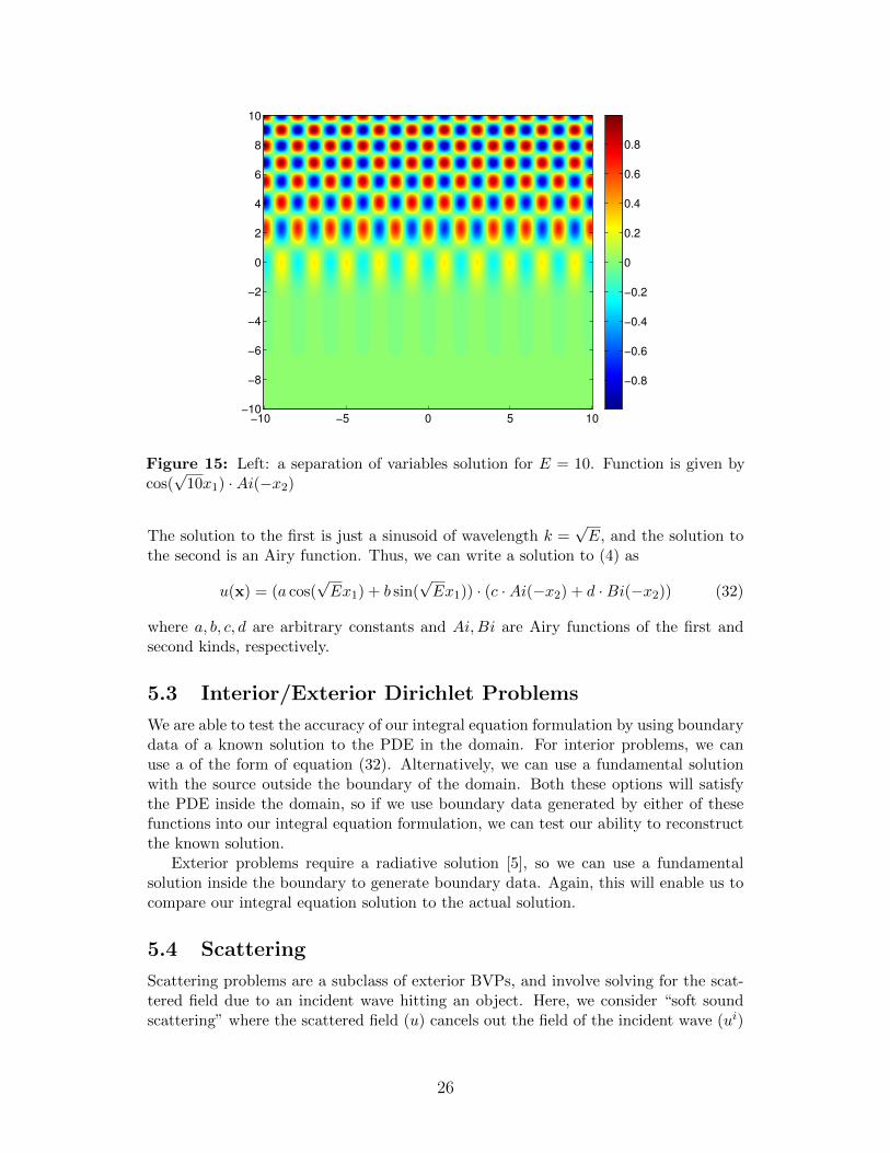
Figure 15: Left: a separation of variables solution for E = 10. Function is given bycos(√

10x1) ·Ai(−x2)

The solution to the first is just a sinusoid of wavelength k =√E, and the solution to

the second is an Airy function. Thus, we can write a solution to (4) as

u(x) = (a cos(√Ex1) + b sin(

√Ex1)) · (c ·Ai(−x2) + d ·Bi(−x2)) (32)

where a, b, c, d are arbitrary constants and Ai,Bi are Airy functions of the first andsecond kinds, respectively.

5.3 Interior/Exterior Dirichlet Problems

We are able to test the accuracy of our integral equation formulation by using boundarydata of a known solution to the PDE in the domain. For interior problems, we canuse a of the form of equation (32). Alternatively, we can use a fundamental solutionwith the source outside the boundary of the domain. Both these options will satisfythe PDE inside the domain, so if we use boundary data generated by either of thesefunctions into our integral equation formulation, we can test our ability to reconstructthe known solution.

Exterior problems require a radiative solution [5], so we can use a fundamentalsolution inside the boundary to generate boundary data. Again, this will enable us tocompare our integral equation solution to the actual solution.

5.4 Scattering

Scattering problems are a subclass of exterior BVPs, and involve solving for the scat-tered field due to an incident wave hitting an object. Here, we consider “soft soundscattering” where the scattered field (u) cancels out the field of the incident wave (ui)

26

0 50 100 150 200 25010

−12

10−10

10−8

10−6

10−4

10−2

100

number boundary points

err

or

0 50 100 150 200 25010

−12

10−10

10−8

10−6

10−4

10−2

number boundary points

err

or

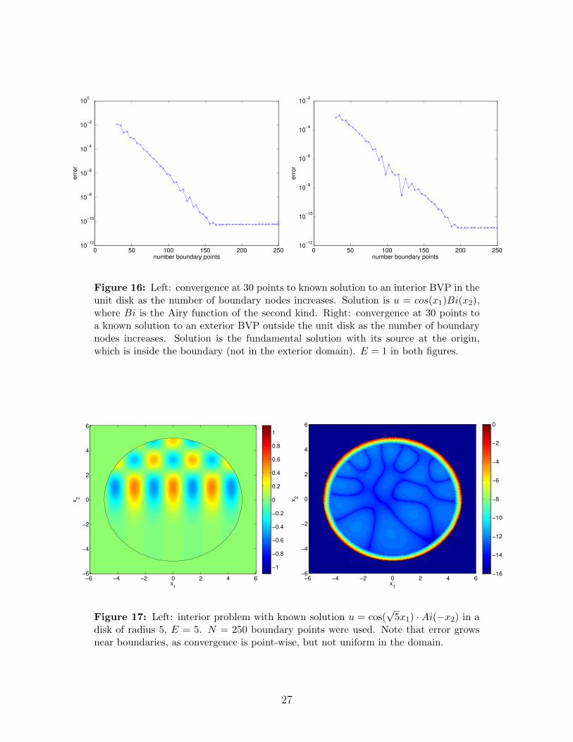
Figure 16: Left: convergence at 30 points to known solution to an interior BVP in theunit disk as the number of boundary nodes increases. Solution is u = cos(x1)Bi(x2),where Bi is the Airy function of the second kind. Right: convergence at 30 points toa known solution to an exterior BVP outside the unit disk as the number of boundarynodes increases. Solution is the fundamental solution with its source at the origin,which is inside the boundary (not in the exterior domain). E = 1 in both figures.

x1

x2

−6 −4 −2 0 2 4 6−6

−4

−2

0

2

4

6

−1

−0.8

−0.6

−0.4

−0.2

0

0.2

0.4

0.6

0.8

1

x1

x2

−6 −4 −2 0 2 4 6−6

−4

−2

0

2

4

6

−16

−14

−12

−10

−8

−6

−4

−2

0

Figure 17: Left: interior problem with known solution u = cos(√

5x1) · Ai(−x2) in adisk of radius 5, E = 5. N = 250 boundary points were used. Note that error growsnear boundaries, as convergence is point-wise, but not uniform in the domain.

27

−30 −20 −10 0 10 20 30−30

−20

−10

0

10

20

30

−0.1

−0.08

−0.06

−0.04

−0.02

0

0.02

0.04

0.06

0.08

0.1

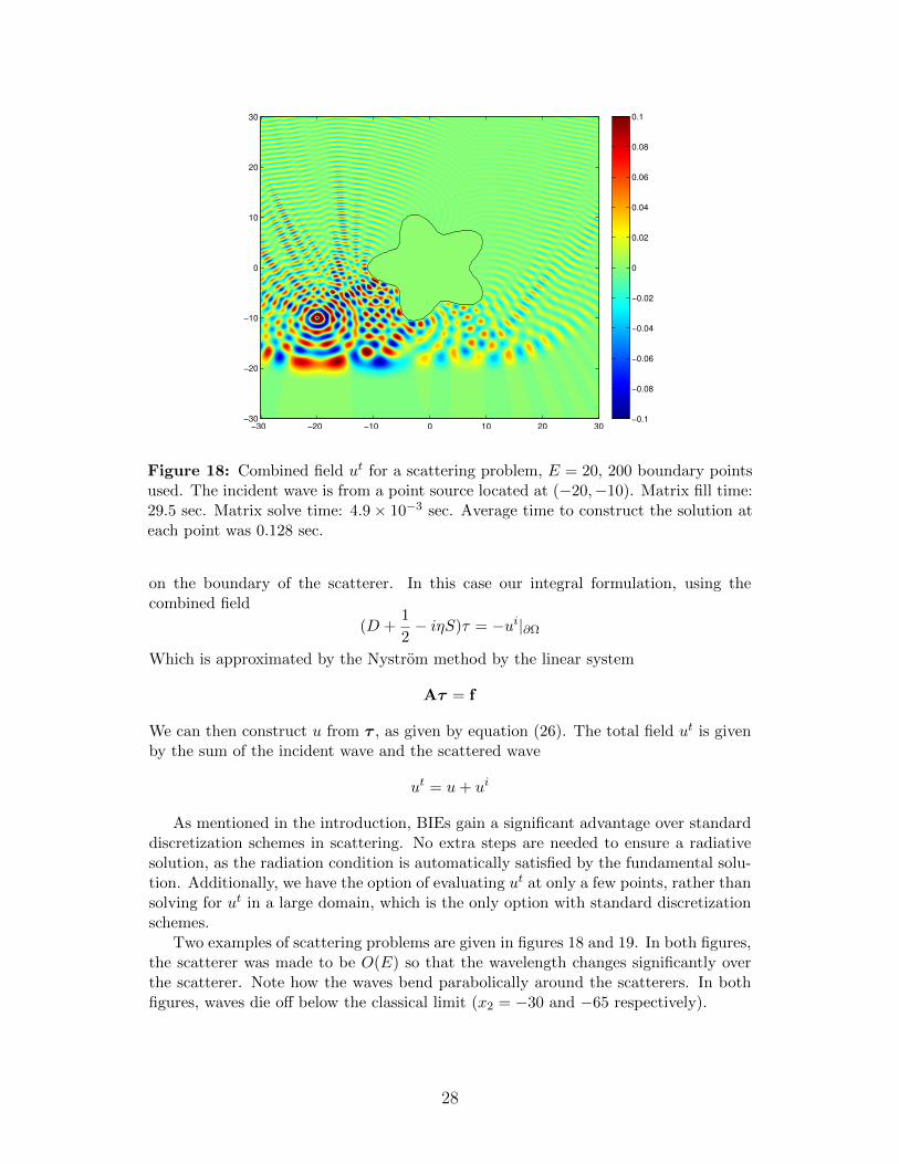
Figure 18: Combined field ut for a scattering problem, E = 20, 200 boundary pointsused. The incident wave is from a point source located at (−20,−10). Matrix fill time:29.5 sec. Matrix solve time: 4.9× 10−3 sec. Average time to construct the solution ateach point was 0.128 sec.

on the boundary of the scatterer. In this case our integral formulation, using thecombined field

(D +1

2− iηS)τ = −ui|∂Ω

Which is approximated by the Nystrom method by the linear system

Aτ = f

We can then construct u from τ , as given by equation (26). The total field ut is givenby the sum of the incident wave and the scattered wave

ut = u+ ui

As mentioned in the introduction, BIEs gain a significant advantage over standarddiscretization schemes in scattering. No extra steps are needed to ensure a radiativesolution, as the radiation condition is automatically satisfied by the fundamental solu-tion. Additionally, we have the option of evaluating ut at only a few points, rather thansolving for ut in a large domain, which is the only option with standard discretizationschemes.

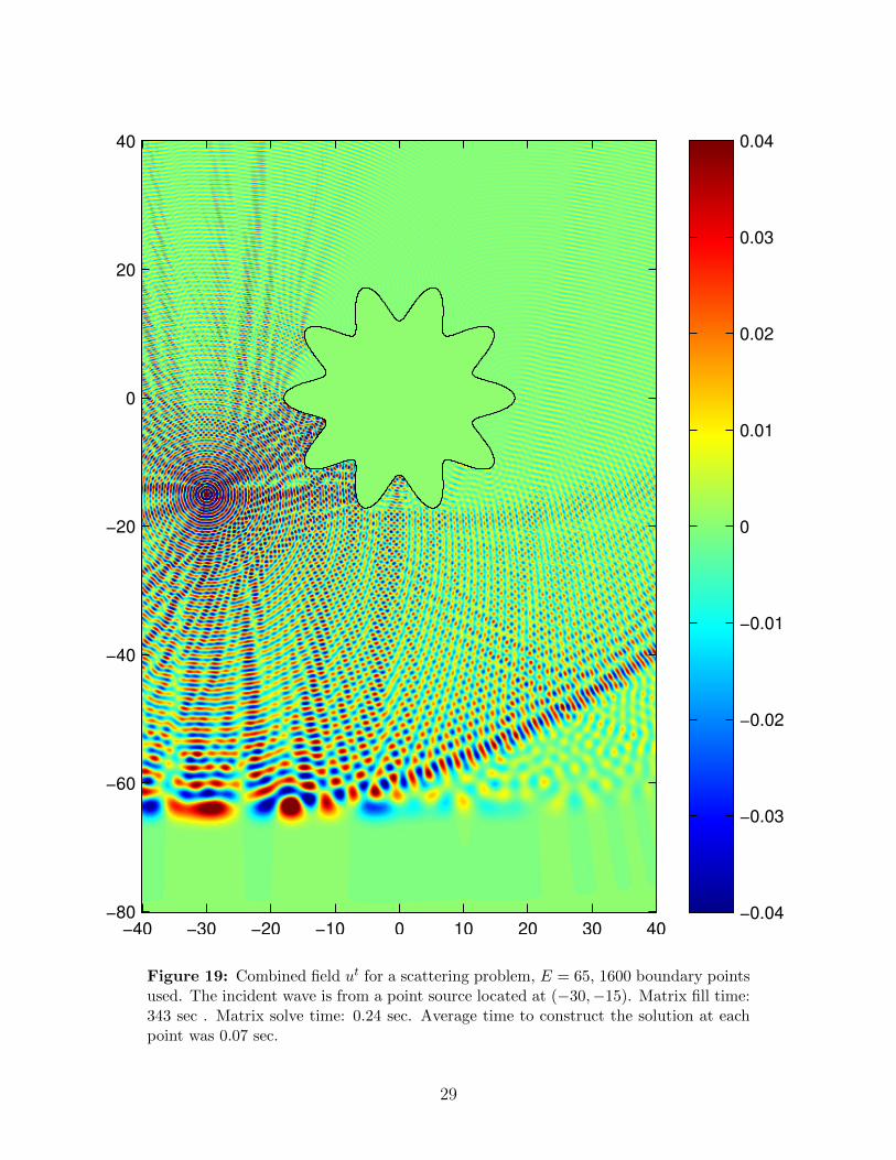
Two examples of scattering problems are given in figures 18 and 19. In both figures,the scatterer was made to be O(E) so that the wavelength changes significantly overthe scatterer. Note how the waves bend parabolically around the scatterers. In bothfigures, waves die off below the classical limit (x2 = −30 and −65 respectively).

28

−40 −30 −20 −10 0 10 20 30 40

−80

−60

−40

−20

0

20

40

−0.04

−0.03

−0.02

−0.01

0

0.01

0.02

0.03

0.04

Figure 19: Combined field ut for a scattering problem, E = 65, 1600 boundary pointsused. The incident wave is from a point source located at (−30,−15). Matrix fill time:343 sec . Matrix solve time: 0.24 sec. Average time to construct the solution at eachpoint was 0.07 sec.

29

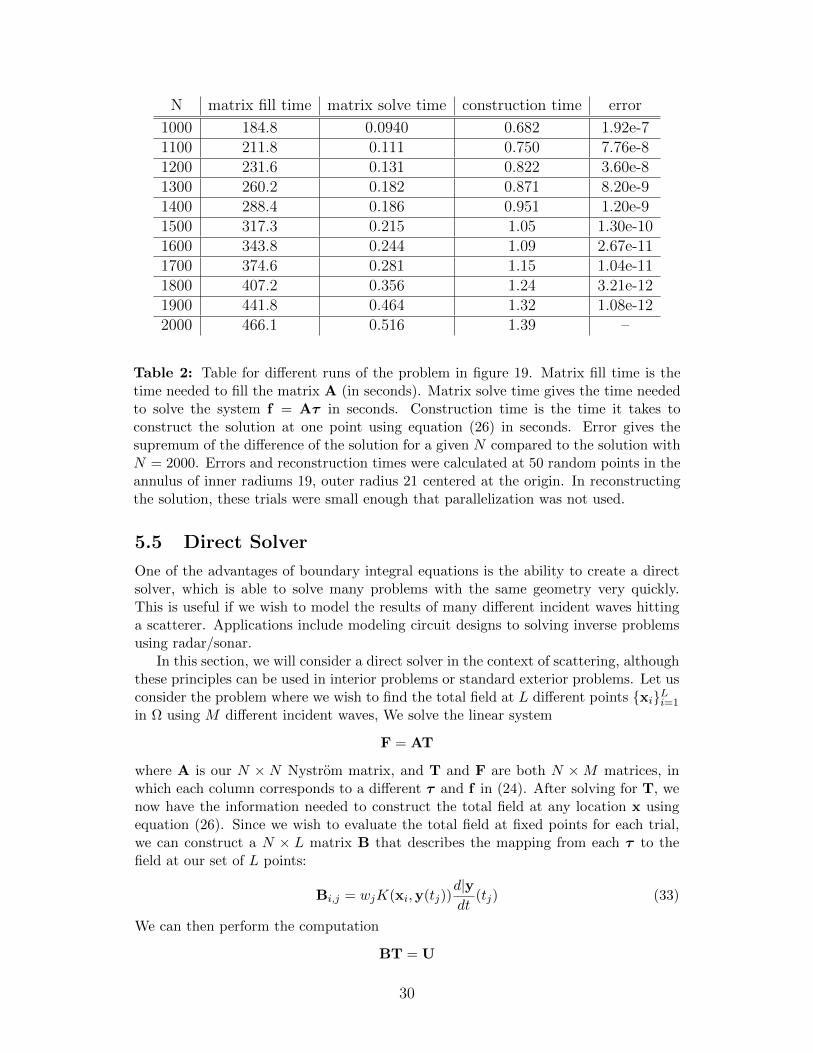
N matrix fill time matrix solve time construction time error

1000 184.8 0.0940 0.682 1.92e-71100 211.8 0.111 0.750 7.76e-81200 231.6 0.131 0.822 3.60e-81300 260.2 0.182 0.871 8.20e-91400 288.4 0.186 0.951 1.20e-91500 317.3 0.215 1.05 1.30e-101600 343.8 0.244 1.09 2.67e-111700 374.6 0.281 1.15 1.04e-111800 407.2 0.356 1.24 3.21e-121900 441.8 0.464 1.32 1.08e-122000 466.1 0.516 1.39 –

Table 2: Table for different runs of the problem in figure 19. Matrix fill time is thetime needed to fill the matrix A (in seconds). Matrix solve time gives the time neededto solve the system f = Aτ in seconds. Construction time is the time it takes toconstruct the solution at one point using equation (26) in seconds. Error gives thesupremum of the difference of the solution for a given N compared to the solution withN = 2000. Errors and reconstruction times were calculated at 50 random points in theannulus of inner radiums 19, outer radius 21 centered at the origin. In reconstructingthe solution, these trials were small enough that parallelization was not used.

5.5 Direct Solver

One of the advantages of boundary integral equations is the ability to create a directsolver, which is able to solve many problems with the same geometry very quickly.This is useful if we wish to model the results of many different incident waves hittinga scatterer. Applications include modeling circuit designs to solving inverse problemsusing radar/sonar.

In this section, we will consider a direct solver in the context of scattering, althoughthese principles can be used in interior problems or standard exterior problems. Let usconsider the problem where we wish to find the total field at L different points xiLi=1

in Ω using M different incident waves, We solve the linear system

F = AT

where A is our N × N Nystrom matrix, and T and F are both N ×M matrices, inwhich each column corresponds to a different τ and f in (24). After solving for T, wenow have the information needed to construct the total field at any location x usingequation (26). Since we wish to evaluate the total field at fixed points for each trial,we can construct a N × L matrix B that describes the mapping from each τ to thefield at our set of L points:

Bi,j = wjK(xi,y(tj))d|ydt

(tj) (33)

We can then perform the computation

BT = U

30

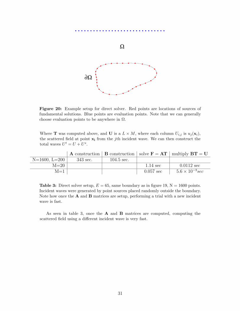
Ω

∂Ω

Figure 20: Example setup for direct solver. Red points are locations of sources offundamental solutions. Blue points are evaluation points. Note that we can generallychoose evaluation points to be anywhere in Ω.

Where T was computed above, and U is a L ×M , where each column Ui,j is uj(xi),the scattered field at point xi from the jth incident wave. We can then construct thetotal waves U t = U + U s.

A construction B construction solve F = AT multiply BT = UN=1600, L=200 343 sec. 104.5 sec.

M=20 1.14 sec 0.0112 secM=1 0.057 sec 5.6× 10−3sec

Table 3: Direct solver setup, E = 65, same boundary as in figure 19, N = 1600 points.Incident waves were generated by point sources placed randomly outside the boundary.Note how once the A and B matrices are setup, performing a trial with a new incidentwave is fast.

As seen in table 3, once the A and B matrices are computed, computing thescattered field using a different incident wave is very fast.

31

6 Conclusion

We have extended the use of boundary integral equations for the first time to Helmholtzboundary value problems in two dimensions where the square of the wavenumber varieslinearly in one coordinate. We have presented a scheme for the numerical evaluationof the fundamental solution (8) first presented by Bracher et al. [3] that is accurateover the x plane, and for a wide range of E. While this scheme’s speed is limited bythe number of quadrature points used in evaluating each point, the scheme is readilyparallelized, which allows for larger computations.

Using this fundamental solution, we have been able to solve boundary value prob-lems where the wavelength changes significantly over the domain, including scatteringproblems with scatterers that are many wavelengths across. Our use of boundary inte-gral equations in solving these problems offers significant advantages to the standarddomain-discretization techniques.

32

References

[1] B. K. Alpert. Hybrid Gauss-trapezoidal quadrature rules. SIAM J. Sci. Comput.,20:1551–1584, 1999.

[2] F. Bornemann and G. Wechslberger. Optimal contours for high-order derivatives.IMA J. Numer. Anal., 33:403–412, 2013.

[3] C. Bracher, W. Becker, S. A. Gurvitz, M. Kleber, and M. S. Marinov. Three-dimensional tunneling in quantum ballistic motion. Am. J. Phys., 66:38–48, 1998.

[4] D. Colton, R. Kress. Integral Equation Methods in Scattering Theory. John Wileyand Sons 1983.

[5] D. Colton, R. Kress. Inverse Acoustic and Electromagnetic Scattering Theory.Springer 1993.

[6] P. R. Garabedian Partial Differential Equations. AMS Chelsea Publishing, 1986.

[7] S. Hao, A. H. Barnett, P. G. Martinsson, and P. Young. High-order accuratemethods for Nystrom discretization of integral equations on smooth curves in theplane.

[8] D. Huybrechs and S. Vandewalle. On the evaluation of highly oscillatory integralsby analytic continuation. SIAM J. Numer. Anal., 44:1026–1048, 2006.

[9] R. Kress. Linear Integral Equations. Springer 1989.

[10] R. J. LeVeque Finite Difference Methods for Ordinary and Partial DifferentialEquations SIAM, 2007.

[11] M. Mahoney. Unpublished notes, 2010.

[12] MPSpack: A MATLAB toolbox to solve Helmholtz PDE, wave scatter-ing, and eigenvalue problems, Barnett A. H. and Betcke T. (2008–2013)http://code.google.com/p/mpspack/

33