DEPARTMENT OF ECONOMICS

An economic model of contagion in interbank

lending markets

Daniel Ladley, University of Leicester, UK

Working Paper No. 11/06 November 2010

Updated December 2010

An economic model of contagion in interbank lending markets

Daniel Ladley

Department of Economics

University of Leicester

United Kingdom

d.ladley@leicester.ac.uk

December 3, 2010

Abstract

This paper examines the relationship between the structure of the interbank lending mar-

ket and systemic risk. We consider a model in which banks finance investment opportunities

through household deposits and borrowing from other banks. Using simulation techniques a

range of interbank markets structures are considered. It is shown that greater levels of inter-

bank connectivity reduce the risk of contagion from the failure of a single bank. In response

to system wide shocks, however, the effect of connectivity is ambiguous, reducing contagion

for small shocks but exacerbating it for larger events. Regulatory changes including forcing

banks to hold more reserves, be less leveraged or constraining the size of borrowing relations

are tested and their effects considered.

Systemic risk, Interbank lending, Regulation, Network, Heterogeneity

G21 C63

1 Introduction

The financial regulation of banks has primarily focused on ensuring that individual institutions

have sufficient funds to protect themselves from the risk of their own investments. The events

of 2007 and 2008 demonstrated the shortcomings of this approach. Problems in a small number

of institutions spread throughout the financial system resulting in the collapse of banks which,

according to regulatory requirements, had adequate capital. Systems which had previously been

thought to encourage stability and permit risk sharing, such as the interbank market, became

a route by which financial distress spread. Banks defaulted on interbank loans’ negatively im-

pacting the balance sheets of their creditors and forcing otherwise sound institutions towards

insolvency and collapse. Fragility became contagious as financial distress spread and strong

banks were brought down by the weak. Institutions were not able to predict who would fail

next and consequently market confidence evaporated. This created a liquidity crisis, preventing

viable institutions from obtaining funds and so exacerbating the system’s problems. Regulators

and governments were forced to intervene to save the system, injecting capital and rescuing

institutions which were judged too-big-to-fail, those who’s bankruptcy could have led to further

damaging cascades of failures. The financial crisis showed that it was not sufficient to regulate

banks in isolation, to protect them against themselves, banks also had to be protected against

each other as the integrity of the system was paramount.

Interbank linkages served to exacerbate the financial crisis by allowing problems to spread

between institutions. In this paper we examine how the structure of the interbank lending

market effects the stability of the financial system1. We consider a model of the behaviour of

heterogenous banks within a closed economy. Households approach banks, placing deposits and

borrowing money for risky projects. Banks interact with each other through interbank market,

obtaining funds but exposing themselves and other banks to counter-party risk and potentially

contagion. The effect of the structure of the interbank market is considered in determining the

conditions under which the risk sharing or contagion inducing effects are dominant.

The model analysed in this paper captures the dynamic nature of the financial system. Funds

are lent from banks to households who invest it in projects which in turn leads to it being rede-

posited into banks, hence within this iterated model money circulates and is multiplied. Banks

1These are not the only inter-bank linkages which can propagate distress. For instance Allen and Carletti(2006) demonstrate how the transfer of credit risk between institutions may lead to contagion whilst Mendozaand Quadrini (2010) show that in a global financial systems a small shock to bank equity may result in a largereduction in asset prices.

2

are presented with a variety of investment opportunities split between loans to households and

loans to other banks. These investments are funded through household deposits and potentially

borrowing from other banks within the system. Each bank’s success is dictated by the perfor-

mance of their investment portfolio. If a bank invests poorly or is unfortunate it may potentially

go bankrupt, if it performs well it will grow. Heterogenous bank sizes arise endogenously within

the model.

It is found that the structure of the interbank market has a significant effect on the ability

of the system to resist contagion in response to system-wide shocks. The optimal structure,

however, is dependent on the magnitude of the shock faced. Markets exhibiting a high degree of

connectivity share the effects of bankruptcy between more counter-parties reducing the proba-

bility of a contagious failure. In contrast, for larger systemic shocks, rather than spreading risk

interbank connections act to propagate the effects of failures. Those market with more interbank

connections become the most vulnerable. Regardless of the size of shock the cost to the deposit

insurer is minimised for the most connected markets as more of the cost of failures is borne

by surviving banks. The effect of higher equity and reserve ratio’s are investigated. Both are

found to decrease the market’s susceptibility to contagion by reducing the number of banks who

cause a second bank to fail. Increasing the equity ratio is found to have a larger effect but at

the cost of reducing the ability of banks to offer credit to households. An alternative regulatory

mechanism, constraining the size of interbank linkages, is also examined. This is found to reduce

the number of bankruptcies whilst increasing the quantity of loans given to households. Care

must be taken in its use, if it is too loose the regulation has no effect, whilst if it is too tight it

severely inhibits the ability of the interbank market to distribute funds efficiently and so reduces

the loans to households.

The model is shown to be robust to perturbations in parameters, producing qualitatively

similar results for a wide range of values. If the constraint of a single interbank rate is relaxed,

such that the rates at which bank’s borrow are conditional on their state the market is found

to be more stable. There is more lending to households and fewer contagious bankruptcies. In

contrast, if banks are allowed to react to the failures of other banks by reducing their confidence

in the interbank market the model economy is found to be less stable. Reducing the efficiency

of the allocation of funds.

The paper is structured as follows: the next section will give an overview of the related

literature on interbank markets. Section 3 will set out a model of a financial system in which

3

banks are potentially susceptible to systemic risk. Section 4 will consider the behaviour of the

model including the potential for contagion under different shocks and a range of market struc-

tures. Section 5 examines the effect of regulation whilst Section 6 relaxes modelling assumptions.

Section 7 concludes.

2 Literature review

The interbank lending market provides a venue for financial institutions to lend funds or borrow

money to meet liquidity or investment requirements. As such it plays an important role in

allowing financial institutions to manage their balance sheets, facilitating the sharing of risk and

the efficient allocation of funds. Whilst the interbank market provides a mechanism for sharing

liquidity risk, participating in the market exposes banks to counter-party risk; The danger is

that a bank is unable to recover lent funds due to the failure of a borrower to repay. In their

influential work, Allen and Gale (2001) model interbank interactions, showing that in equi-

librium banks will optimally insure themselves against liquidity shocks by holding deposits in

other banks. This protection, however, makes them potentially vulnerable to the failures of their

counter-parties. If a very large shock strikes a single bank, which exceeds its available funds,

the bank may collapse eliminating a portion of the counter-parties’ deposits. If the impact of

this bankruptcy is sufficiently large it may potentially cause the default of further, otherwise

healthy, banks which may in turn affect others. The effect of these contagious events may be

very severe (Gai and Kapadia, 2010), resulting in a loss of equity (Eisenberg and Noe, 2001)

and may potentially justify government or regulatory intervention (Kahn and Santos, 2010)2.

The majority of trading in the interbank-market happens over-the-counter (OTC), directly

between pairs of banks, as opposed to via a central counter-party. Unlike trades for equities

which result in the instantaneous transfer of ownership, interactions within the interbank mar-

ket generally last for an extended period. Funds are initially borrowed by one bank and repaid

over a length of time which can range from overnight for certain classes of borrowing, up to

periods of several years. At any point a particular bank may be involved in multiple lending

or borrowing relationships and as such may be connected to multiple counter-parties. Across

all banks these linkages form a structure which may be described by a weighted, directed graph

in which nodes are financial institutions and edges are lending relationships of a specific value.

2Also see Giesecke and Weber (2006), Elsinger et al. (2006) and Brusco and Castiglionesi (2007) for alternativeviews.

4

Iori et al. (2008) use graph theoretic measures to analyse the structure of the Italian interbank

market. They show that the structure of the market is characterised by the existence of large

‘hub’ banks with which many of the market participants interact. The market is also found to

be relatively efficient, there being few opportunities to borrow from one institution and lend to

another profitably. The structure is shown to vary over time. Towards the end of the month

the density of connections increases as banks increase their borrowing and lending to meet their

monthly capital requirements. Using similar techniques, Cocco et al. (2009) show that banks

tend to form relationships with other institutions that have negative correlated liquidity shocks.

The structure of interbank markets, the numbers and distribution of linkages together with

their size, has a large effect on how shocks spread and the markets potential susceptibility to

systemic events (Leitner, 2005; Muller, 2006). Initially, if a single institution fails only those

banks to which it owes money suffer directly, the remainder of the system is unaffected3. The

direct impact may cause one or more of the initial counter-parties to fail which can harm other

institutions within the system. Muller (2006) and Upper and Worms (2004), by analysing data

for the Swiss and German banking systems respectively, show that in both cases there is signif-

icant potential for this to occur. Highly centralised markets, those with a few large hub banks,

are shown to be particularly susceptible to this risk. For instance the UK interbank market,

which exhibits tiering (Becher et al., 2008), may fall into this category.

Angelini et al. (1996), for the Italian interbank market, and Boss et al. (2004), for the

Austrian interbank market draw a different conclusion. They find that there is relatively little

danger of systemic events. Only a very small number of banks could cause other banks to

fail if they themselves defaulted. This difference in conclusions is, at least in part, driven by

differences in the interbank markets. Each of the empirical studies provides a snapshot of a

particular market at a particular time under particular financial conditions and is not a general

assessment of the susceptibility of interbank markets to contagion. The markets studied have

different structures, for instance as Angelini et al. (1996) note, the volume traded varies to a

large extent across countries. In order to make a complete assessment it would be necessary to

perform a large number of similar studies on a range of markets and situations. Unfortunately,

the information to conduct such empirical investigations is often impossible to acquire. For

each of the empirical investigations it was necessary to know (or estimate) both the financial

3For the present we ignore issues regarding market confidence and beliefs. In reality, a bank that is notdirectly effected may still fear for their investments and alter their portfolio to limit the possibility of futurelosses. See Lagunoff and Schreft (2001) for an example of this mechanism.

5

position of each market participant and crucially each participant’s lending relationships. Whilst

the financial positions may be estimated from public balance sheet data, information regarding

financial relationships is often proprietary and consequently much harder to collect. In most

cases interbank lending transactions are conducted directly between institutions, frequently by

phone call rather than through an automated exchange4. So in contrast to many equities markets

where a central body collects trading data, within these markets no single body has a complete

picture of all transactions. This means that empirical studies are restricted to a relatively small

number of countries and occasions where this data is available.

Theoretical studies have complemented empirical work in understanding the determinants of

systemic risk. Work in this area has shown that there is a relationship between market structure

and the effect and scope of financial contagion (e.g. Leitner, 2005), however, the nature of this

relationship is ambiguous. Vivier-Lirimont (2006), in a model based on the Diamond and Dybvig

(1983) paradigm, find that longer path lengths between banks, higher reserve levels and higher

liquidation values reduce the severity of contagious events. Increasing the number of interbank

connections increases severity. This result is partially supported by Brusco and Castiglionesi

(2007) who show that increasing cross-holdings increase the extent of contagion but reduces the

effect on individual institutions. It differs, however, from Giesecke and Weber (2006) who find

that more connections reduce contagion. Boss et al. (2004) demonstrate that the betweenness of

a bank, a graph theoretic measure of how central a bank is in a network, is correlated with the

contagious effect of its default. Using simulation techniques Nier et al. (2007) show that a small

increase in connectivity increases systemic risk but beyond a certain point the degree of systemic

risk decreases. In contrast, Lorenz and Battiston (2008) and Battiston et al. (2009) find the op-

posite relationship, the scale of bankruptcies is minimised for intermediate levels of connectivity.

Battiston et al. (2009) attribute this effect to the actions of the financial accelerator, whereby de-

terioration of a banks financial position causes further deterioration in future time periods. For

example the creditors of a bank which suffers a loss may impose tighter credit conditions further

harming the banks’ position. Without the financial accelerator they find increasing connectivity

reduces bankruptcy. The results above highlight the trade off discussed by Allen and Gale (2001)

of risk sharing versus contagious vulnerability. Whilst sparser networks limit the ability of shocks

to spread, reducing contagion, they also reduce the risk sharing capacity of the market and so

increase the risk of individual banks failing. This finding is highlighted by Iori et al. (2006) who

4The Italian interbank system being a notable exception in that quoted interest rates and transactions gothrough a central computer system.

6

show that in the presence of heterogenous banks the interbank market permits a crisis in one

bank to spread, however, it also provides stabilisation meaning the overall effect is ambiguous.

This ambiguity makes it difficult to designing regulations to limit systemic events within

the interbank market. The Basel III reforms emphasise increasing regulatory capital to provide

banks with a larger buffer (and additionally less leverage) in the event of future failures. Rochet

and Tirole (1996) highlight the benefits of monitoring to reduce the probability of contagious

events whilst Freixas et al. (2000) considers the costs of failures and interventions. The model

presented in this paper will consider the susceptibility of different interbank market architectures

to small and system-wide shocks. Demonstrating how the susceptibility to contagious events

varies with market structure along with the effectiveness of different regulatory approaches in

limiting the size of failures.

3 Model

We consider a discrete time model of the behaviour of a closed economy containing N banks

and M households. Each bank, i, has a balance sheet comprising equity (Ei), deposits (Di),

cash reserves (Ri), loans to the non-bank sector (Li) and loans to the other banks (Ii)5. Whilst

each household, j, holds depositable funds (dj). Both households and banks occupy locations on

the circumference of a unit circle. This circle represents a dimension, not necessarily physical,

on which the agents differ, effecting their ability to attract household deposits and borrowing.

Banks are equidistantly spaced with bank 1 being located at the top of the circle and the remain-

ing banks arrayed in index order clockwise around the circumference. The same arrangement is

followed by households with household 1 being at the top of the circle.

3.1 Deposits and Lending

At the start of each time period each bank publically declares its deposit interest rate, rdepositi ,

and lending interest rate, rloani . Each household places all of its depositable funds in the bank

which maximises its expected return, specifically:

arg maxi∈N

dj(rdepositi − g(i, j)) (1)

Where g(i, j) is a function giving the distance between i and j6. If no i exists such that

5Positive values correspond to lending, negative to borrowing.6In line with the majority of the previous literature employing circular city hotelling mechanisms (e.g. Salop,

7

Equation 1 is positive the household retains its funds and earns no interest. Bank deposits are

insured by an agent outside of the system who guarantees that households will be repaid the full

value of their deposits in the event of bank failure. Households are, therefore, not concerned with

the risk of bank default and so select the bank offering the highest return. We model households

as being highly active in their management of deposits, however, in reality deposits tend to be

sticky. Individuals are slow to respond to changes in interest rates, frequently maintaining their

deposits in institutions paying suboptimal rates, rather than switching7.

After allocating deposits, each household is presented with a single limited liability invest-

ment opportunity, ltj . Each opportunity requires an initial investment of a single unit of currency

at time t and provides a payoff to the household at time t + 2 of µ with probability θltj. With

probability 1−θltjthe investment provides zero payoff8. A household with an investment oppor-

tunity must fund the investment through borrowing from a bank. We assume that households

wish to retain their deposits for consumption but will invest in the limited liability opportu-

nity to increase their utility9. Each household approaches a single bank which maximise the

household’s expected return:

arg maxi∈N

θltj(µ − (1 + rloan

i )2) − g(i, j) (2)

Investment opportunities are limited liability; in the event of the zero payoff state banks

do not have a claim to the households deposits. Consequently if bank i funds an investment

opportunity, ltj , with probability θltjthe bank receives (1 + rloan

i )2 at time t + 2 whilst with

probability 1 − θltjthe bank receives nothing. If no i exists such that Equation 2 is positive no

funding request is made and the opportunity goes unfunded.

3.2 Investment Behaviour

Each time step, banks determine the allocation of assets and liabilities on their balance sheets.

Money is distributed from household deposits and interbank borrowing to fund loans to house-

holds, interbank lending and to save as cash reserves. Banks are constrained in this allocation by

1979) we assume that transaction costs are linear in the distance between two actors.7Experiments were performed in which deposits were sticky - depositors only moved their deposits with a

fixed probability. Values of this probability greater than 0.02 produced no significant difference in results.8Details of why two period investments are used are provided in the next section.9An alternative formulation would additionally include firms. Households would place deposits, whilst firms,

without any cash holdings, would approach banks to fund investment opportunities. This formulation is identicalin operation to the model presented above, it simply separates the deposit and investment behaviours of thenon-bank agents.

8

regulation along with their current holding of two period loans and borrowing from the previous

time step.

We consider banks to be victims of a classical principal agent problem. The owners of banks

wish to maximise returns in the long term, however, due to imperfect contracting the managers

they employ are focused on short term returns. This captures a common observation that bank

traders and managers receive substantial bonuses for short term performance, encouraging them

to take on excess risk and be focused on short term returns. Within this model we do not con-

sider the identity of the owners or the managers, we are concerned only with the effect of this

relation on bank behaviour. Banks are solely interested in maximising short term returns. They

do not refuse investment opportunities in the current period and save funds based on the belief

that they will receive better opportunities in the future. Banks, therefore, behave as myopic,

risk neutral, expected return maximisers.

In allocating their portfolios banks are subject to five key constraints. The first constraint,

given by Equation 3, states that each bank’s balance sheet must balance; i.e. assets are equal

to liabilities.

Li + Ri + Ii = Ei + Di (3)

The second constraint given in Equation 4 fixes the value of the deposit term on the balance

sheet. It specifies that the bank’s holding of deposits is equal to the sum of deposits placed in

that bank by households. The bank may neither refuse deposits nor gain access to additional

deposits outside of those contributed by households.

Di =M∑

j=1

dj where i = arg maxi∈N

dj(rdepositi − g(i, j)) (4)

The third constraint, Equation 5, governs the level of liquid cash reserves which the bank

holds. The reserve ratio is given by αi, the bank’s preference for cash reserves. Whilst this

parameter may be set to any level, regulation imposes a minimum level of liquid cash reserves,

forcing the bank to hold at least fraction αg.

Ri ≥ max(αg, αi)Di (5)

The fourth constrain given by Equation 6 specifies a maximum equity to risky assets ratio.

9

In this equation βi is the bank’s preferred equity ratio and βg is a minimum value imposed by

regulation. The max operator means only interbank loans and not borrowing are considered.

Note, whilst reserves are assets, they are not included in the equity ratio. This is because under

the Basel accords they are judged to have a risk-weight of zero and so are not included in cap-

ital adequacy calculations. In this model interbank lending and household lending are equally

weighted in the risk calculation.

Ei ≥ max(βg, βi)(Li + max(Ii, 0)) (6)

The constraint given in Equation 7 states that the amount invested in loans is equal to the

total funds invested in individual projects. Here, Kti is the set of investments funded by bank i

in period t and we define ‖.‖ to be the sum of the values of loans in the included set. Importantly

this constraint includes all projects funded at time t but also those that were funded at time

t − 1. Deposits and reserves may be reallocated at every time step, however, like investment

opportunities, loans between banks last for two time steps. Once a loan contract (either to a

bank or non-bank has been entered into) it may not be sold or completed prior to its scheduled

end date; as such they are illiquid assets.

Li = ‖Kti‖ + ‖Kt−1

i ‖ (7)

When calculating the optimal portfolio the level of equity of each bank is given by its state.

The constraints above fix the value of deposits whilst the quantity of reserves are specified by

the reserve ratio. Consequently the key choice for banks is the distribution of funds between

interbank lending and loans to households. In making this decision bank i determines the com-

position of Kti the set of investment opportunities which it funds. The loans are selected from

P ti , the set of investment opportunities presented to bank i by households at time t, i.e. Kt

i ⊆ P ti .

The expected return for the bank from each loan, ltj , may be expressed as θtj(1 + rloan

i )2 − 1.

Bank’s invest in loans in decreasing order of return until the expected return falls below zero or

the bank runs out of funds. If the bank runs out of suitable loan opportunities whilst it still has

available funds the bank may lend to other institutions subject to the expected return of the

loan being positive. Alternatively if a bank has excess loan opportunities it may borrow money

from other banks to fund these investments. Each time step, each bank, i, determines its allo-

cation of funds between investment projects and interbank lending and borrowing to maximise

10

its expected return, E(ri) given by:

E(ri) = (

Kti

∑

kti=1

θkti(1 + rloan

i )2 − 1) + Iti ((1 + rinterbank)2f(It

i ) − 1) (8)

Where θkti

is the repayment probability for loan kti (remember each loan is of unit size) and

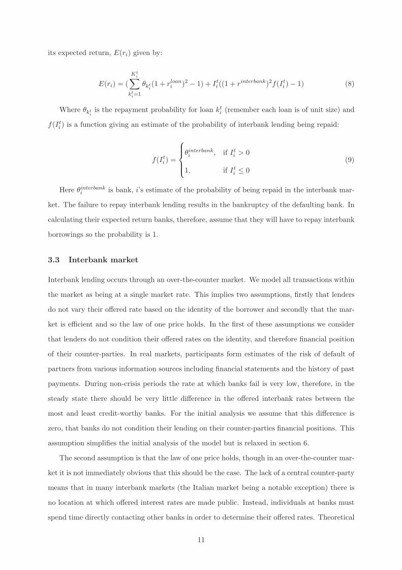
f(Iti ) is a function giving an estimate of the probability of interbank lending being repaid:

f(Iti ) =

θinterbanki , if It

i > 0

1, if Iti ≤ 0

(9)

Here θinterbanki is bank, i’s estimate of the probability of being repaid in the interbank mar-

ket. The failure to repay interbank lending results in the bankruptcy of the defaulting bank. In

calculating their expected return banks, therefore, assume that they will have to repay interbank

borrowings so the probability is 1.

3.3 Interbank market

Interbank lending occurs through an over-the-counter market. We model all transactions within

the market as being at a single market rate. This implies two assumptions, firstly that lenders

do not vary their offered rate based on the identity of the borrower and secondly that the mar-

ket is efficient and so the law of one price holds. In the first of these assumptions we consider

that lenders do not condition their offered rates on the identity, and therefore financial position

of their counter-parties. In real markets, participants form estimates of the risk of default of

partners from various information sources including financial statements and the history of past

payments. During non-crisis periods the rate at which banks fail is very low, therefore, in the

steady state there should be very little difference in the offered interbank rates between the

most and least credit-worthy banks. For the initial analysis we assume that this difference is

zero, that banks do not condition their lending on their counter-parties financial positions. This

assumption simplifies the initial analysis of the model but is relaxed in section 6.

The second assumption is that the law of one price holds, though in an over-the-counter mar-

ket it is not immediately obvious that this should be the case. The lack of a central counter-party

means that in many interbank markets (the Italian market being a notable exception) there is

no location at which offered interest rates are made public. Instead, individuals at banks must

spend time directly contacting other banks in order to determine their offered rates. Theoretical

11

work, however, suggests this limited communication may be sufficient for the market to converge

to the equilibrium price (e.g. Axtell, 2005). Here we assume that there is sufficient information

exchanged for the market to identify a single price. Empirically this is also supported by Iori

et al. (2008) who show that the Italian interbank market is efficient in this manner.

The interbank rate is dependent on the lending and borrowing preferences of individual banks

which are determined by the portfolio optimization set out above. This optimization itself is

specific to each individual bank and dependent on the interbank rate. There is no closed form

solution for the equilibrium, therefore in order to identify the market rate and simultaneously

solve the bank optimization problems it is necessary to use a computational approach. Here we

use a bi-section method. This operates by taking an interval in which the interest rate is known

to lie and calculating the supply and demand at the midpoint. The interval is then halved to

lie between the mid point and either the previous maximum or minimum depending on whether

supply or demand are in excess. Iterative application of this algorithm leads to an increasingly

small interval in which the equilibrium interest rate lies. Here we calculate the interval such

that it is no larger than 10−6 and the midpoint taken as the market rate.

Unfortunately it is not guaranteed that there is an interest rate at which supply is exactly

equal to demand. The market contains a finite number of investments each requiring one unit

of funds. Consequently the amounts of money individual banks wish to lend or borrow changes

in discrete steps. It is guaranteed, however, that the supply and demand functions cross at most

once, since each individual bank’s demand for (supply of) funds is downward (upward) sloping.

Under these conditions the best the algorithm can guarantee is to identify a small region in

which excess demand changes to excess supply. If supply and demand do not exactly balance

the minimum interest rate which sets excess demand to zero is selected. Any excess funds held

by lenders are placed in cash reserves.

In over-the-counter markets, transactions are bilateral, when a bank lends money it lends to

one (or more) specific counter-parties who must repay the lender. If those banks go bankrupt the

lender may not be repaid. The introduction detailed results showing that a markets susceptibil-

ity to systemic shocks was effected by its structure of interbank connections. Within this model

the pattern of interbank lending connections are determined exogenously allowing a range of

interbank market structures to be investigated and compared to different real world examples10.

We consider the model for different values of λ, the probability that a given lender lends money

10A future development of this model would be to make connection decisions endogenous with the desire offinding an optimal interbank market structure under a given set of conditions.

12

to a particular borrower. As λ increases the density of interbank connections also increases.

The interbank connections are constructed as follows. Initially we partition the population of

banks into three sets based on their desired interbank positions for the current period: lenders,

borrowers and those with no position. Each member of the set of lenders is considered in turn

in decreasing order of the magnitude of funds offered. A set of potential counter-parties, Ci, is

constructed for the lender i, where each member of the set of borrowers is added to, Ci with prob-

ability λ. The total demanded funds of the borrowers in set Ci are calculated and if this value is

less than the funds offered, new borrowers are added. Borrowers not in the set Ci are added one

at a time in decreasing order of magnitude of funds demanded until the total value of funds re-

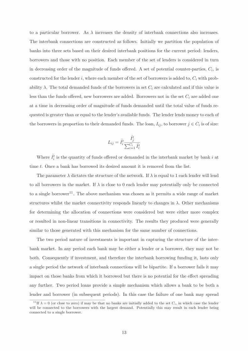
quested is greater than or equal to the lender’s available funds. The lender lends money to each of

the borrowers in proportion to their demanded funds. The loan, Iij , to borrower j ∈ Ci is of size:

Lij = Iti

Itj

∑Ci

c=1Itc

Where Iti is the quantity of funds offered or demanded in the interbank market by bank i at

time t. Once a bank has borrowed its desired amount it is removed from the list.

The parameter λ dictates the structure of the network. If λ is equal to 1 each lender will lend

to all borrowers in the market. If λ is close to 0 each lender may potentially only be connected

to a single borrower11. The above mechanism was chosen as it permits a wide range of market

structures whilst the market connectivity responds linearly to changes in λ. Other mechanisms

for determining the allocation of connections were considered but were either more complex

or resulted in non-linear transitions in connectivity. The results they produced were generally

similar to those generated with this mechanism for the same number of connections.

The two period nature of investments is important in capturing the structure of the inter-

bank market. In any period each bank may be either a lender or a borrower, they may not be

both. Consequently if investment, and therefore the interbank borrowing funding it, lasts only

a single period the network of interbank connections will be bipartite. If a borrower fails it may

impact on those banks from which it borrowed but there is no potential for the effect spreading

any further. Two period loans provide a simple mechanism which allows a bank to be both a

lender and borrower (in subsequent periods). In this case the failure of one bank may spread

11If λ = 0 (or close to zero) if may be that no banks are initially added to the set Ci, in which case the lenderwill be connected to the borrowers with the largest demand. Potentially this may result in each lender beingconnected to a single borrower.

13

further through the interbank market, potentially affecting banks which are not linked to the

initial failure. This allows richer and potentially more realistic contagious events than would be

possible in the one period model.

3.4 Model Operation

This section details the order of events within each time period in the model. At the start of

period t, interest is paid to households on their deposits established during period t− 1. Banks

pay to households to the amount of interest defined in Equation 1. After interest is paid, loan

success is evaluated for loans established in period t − 2 and banks repaid by households as

appropriate. The interbank lending from time t − 2 which funded these investments is then

repaid. If after interest payments and loan success have been evaluated the bank has negative

equity it is declared bankrupt. Similarly if a bank has insufficient cash reserves to repay its

interbank debts it is declared bankrupt and its creditors are repaid in proportion to the size of

their debt up to the bank’s available cash reserves. If a bank is not fully repaid it suffers a loss

in equity which may, potentially cause it to go bankrupt. If this occurs any interbank borrowing

on its balance sheet is resolved in the same manner. As such the failure of one bank may spread

to its counter-parties and then further within the system.

If a bank fails to which a household or bank owes money, the borrower is still required to

repay its loan at the appropriate due date. This is consistent with an administrator ensuring

creditors of a bank meet their requirements. Any funds arising from such repayments are con-

sidered to either be absorbed by the administrators of the failed bank or to go to the deposit

insurer to cover their expenses. This is reflected in Equation 9. After loans and bankruptcies

have been resolved the deposits each household possess at time t are set such that:

dtj =

∑Ni=1

Lt−1

i

M(10)

i.e. the total loans from the previous time step are equal to the cash holdings of households

available for deposits at the current time step. Money is transferred between households as part

of the operation of the real economy. When funds are lent to a household to invest, goods or

services are purchased resulting in monetary transfers. In this paper we do not consider the detail

and distribution of these interactions and so we assume that funds are distributed uniformly12.

12Alternative mechanisms including having no redistribution and time varying distributions were tested buthad little effect on the results.

14

At this point households place their deposits in banks. Banks then allocate their funds as

described above and the interbank rate is calculated along with the lending and borrowing re-

lationships. Finally at the end of each period an inflationary process is applied to all values

(including cash, loans, reserves etc.) at the following rate:

F t =

∑Ni=1

Eti

N− 1 (11)

The effect of the inflationary process is to maintain a fixed value of equity within the system.

Doing so simplifies both the analysis and the computational process13. An alternative approach

would be to model growth of the real economy, increasing the quantity and value of loan request

each time step and modelling projects as reallocating and potentially consuming wealth along

with creating it. The complexity of this approach together with the many necessary assumptions

would complicate the analysis of the model without necessarily adding additional insight.

3.5 Parameters and Learning

Banks optimise their portfolios each time step to achieve the maximum expected return. There

are, however, several parameters which affect this allocation along with the behaviour and prof-

itability of the bank. These parameters are: reserve ratio, equity ratio, lending interest rate,

deposits interest rate and level of confidence in interbank lending. There is no closed form

solution for assigning optimal values to these parameters within this model with time varying

heterogenous banks and under different regulatory frameworks. The values of these parame-

ters are set by a genetic algorithm, an optimization process by which less profitable parameter

combination are replaced by those which produce higher returns.

Genetic algorithms (GAs) were first brought to prominence by the work of Holland (1975).

They use mechanisms based on the theory of evolution, such as selection and mutation, to find

optimise solutions to problems. A genetic algorithm maintains a population of candidate solu-

tions. Each of these solution comprises a vector of values which encodes a particular solution

to the problem. In every generation each candidate is evaluated and assigned a score against

some criteria. The highest scoring are copied into a new population subject to mutation, small

perturbations of the parameter values, and crossover, the combination of two candidate solutions

to produce a new solution. This mechanism is repeated over time, resulting in increasingly ‘fit’

solutions to the problem to be found.

13Without this terms within the model could potentially grow to infinity and prevent a solution being found.

15

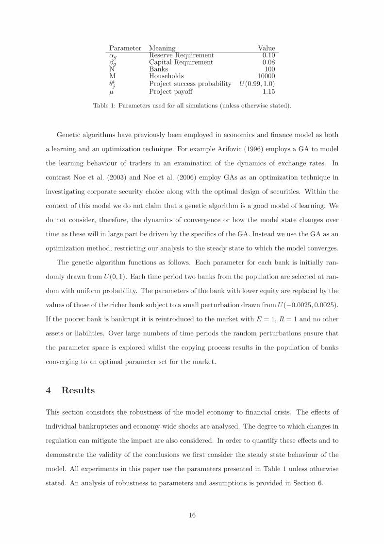
Parameter Meaning Valueαg Reserve Requirement 0.10βg Capital Requirement 0.08N Banks 100M Households 10000θtj Project success probability U(0.99, 1.0)

µ Project payoff 1.15

Table 1: Parameters used for all simulations (unless otherwise stated).

Genetic algorithms have previously been employed in economics and finance model as both

a learning and an optimization technique. For example Arifovic (1996) employs a GA to model

the learning behaviour of traders in an examination of the dynamics of exchange rates. In

contrast Noe et al. (2003) and Noe et al. (2006) employ GAs as an optimization technique in

investigating corporate security choice along with the optimal design of securities. Within the

context of this model we do not claim that a genetic algorithm is a good model of learning. We

do not consider, therefore, the dynamics of convergence or how the model state changes over

time as these will in large part be driven by the specifics of the GA. Instead we use the GA as an

optimization method, restricting our analysis to the steady state to which the model converges.

The genetic algorithm functions as follows. Each parameter for each bank is initially ran-

domly drawn from U(0, 1). Each time period two banks from the population are selected at ran-

dom with uniform probability. The parameters of the bank with lower equity are replaced by the

values of those of the richer bank subject to a small perturbation drawn from U(−0.0025, 0.0025).

If the poorer bank is bankrupt it is reintroduced to the market with E = 1, R = 1 and no other

assets or liabilities. Over large numbers of time periods the random perturbations ensure that

the parameter space is explored whilst the copying process results in the population of banks

converging to an optimal parameter set for the market.

4 Results

This section considers the robustness of the model economy to financial crisis. The effects of

individual bankruptcies and economy-wide shocks are analysed. The degree to which changes in

regulation can mitigate the impact are also considered. In order to quantify these effects and to

demonstrate the validity of the conclusions we first consider the steady state behaviour of the

model. All experiments in this paper use the parameters presented in Table 1 unless otherwise

stated. An analysis of robustness to parameters and assumptions is provided in Section 6.

16

Model Type Value SD Empirical Type Normalised RealLoans 391.5 (32.6) Loans 950.2 8330.1Interbank Loans 283.3 (36.9) Interbank Loans 41.5 364.5Reserves 34.8 (3.42) Cash Assets 36.3 317.1Unused capital 14.3 (6.8)

Other Assets 94.55 829.0Deposits 341.3 (31.1) Deposits 721.8 6327.3

Borrowings 221.7 1943.9Other Liabilities 71.9 630.1

Equity 99.1 (5.13) Residual 99.1 868.7

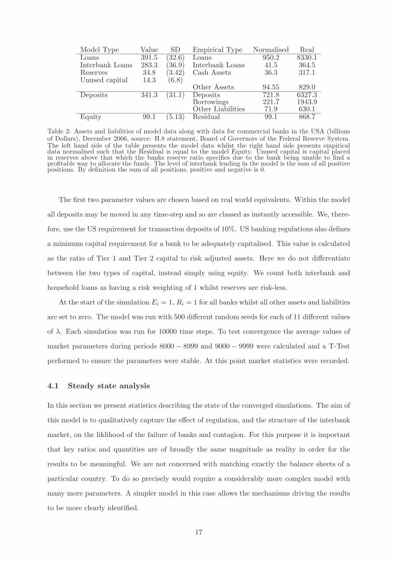
Table 2: Assets and liabilities of model data along with data for commercial banks in the USA (billionsof Dollars), December 2006, source: H.8 statement, Board of Governors of the Federal Reserve System.The left hand side of the table presents the model data whilst the right hand side presents empiricaldata normalised such that the Residual is equal to the model Equity. Unused capital is capital placedin reserves above that which the banks reserve ratio specifies due to the bank being unable to find aprofitable way to allocate the funds. The level of interbank lending in the model is the sum of all positivepositions. By definition the sum of all positions, positive and negative is 0.

The first two parameter values are chosen based on real world equivalents. Within the model

all deposits may be moved in any time-step and so are classed as instantly accessible. We, there-

fore, use the US requirement for transaction deposits of 10%. US banking regulations also defines

a minimum capital requirement for a bank to be adequately capitalised. This value is calculated

as the ratio of Tier 1 and Tier 2 capital to risk adjusted assets. Here we do not differentiate

between the two types of capital, instead simply using equity. We count both interbank and

household loans as having a risk weighting of 1 whilst reserves are risk-less.

At the start of the simulation Ei = 1, Ri = 1 for all banks whilst all other assets and liabilities

are set to zero. The model was run with 500 different random seeds for each of 11 different values

of λ. Each simulation was run for 10000 time steps. To test convergence the average values of

market parameters during periods 8000 − 8999 and 9000 − 9999 were calculated and a T-Test

performed to ensure the parameters were stable. At this point market statistics were recorded.

4.1 Steady state analysis

In this section we present statistics describing the state of the converged simulations. The aim of

this model is to qualitatively capture the effect of regulation, and the structure of the interbank

market, on the liklihood of the failure of banks and contagion. For this purpose it is important

that key ratios and quantities are of broadly the same magnitude as reality in order for the

results to be meaningful. We are not concerned with matching exactly the balance sheets of a

particular country. To do so precisely would require a considerably more complex model with

many more parameters. A simpler model in this case allows the mechanisms driving the results

to be more clearly identified.

17

Table 2 shows the average asset and liability holdings of all banks within the model economy,

together with the balance sheets of all American commercial banks in 2006. Here pre-financial

crisis data were chosen as it is compared to pre-shock model data. Balance sheet terms are

matched to their closest equivalent, but due to the richness and additional complexity of the

real economy this is not possible for all values. In this, and all subsequent tables, the level of

interbank loans is the total funds lent, the sum of positive positions. The sum of all positions

within the market would be 0 as interbank lending is equal to interbank borrowing within this

closed economy.

The ratio of loans to deposits is similar in both the model and empirical data. Relative to

equity, however, both of these values are too small in the model. This is a consequence of the

inflationary process. In order to maintain a fixed level of equity for computational tractability

a relatively high rate of inflation (on average 13%) is necessary. This reduces the value of loans

and deposits each time step. This effect is cumulative as loans at time t are used to calculate

deposits at time t + 1. Consequently when inflation along with reserve requirements are taken

into account the maximum (post inflation) value of loans possible within the model is:

0.87∞

∑

t=0

100 × 0.87t × 0.9t ≈ 401

This value is very close to the observed value of loans and unused capital. Bank’s preferred

equity ratio and reserve ratios (Table 3) are both less than the values specified by the regulations

i.e. 8% and 10%. This means that the regulated values are used in all cases and the banks are

maximally leveraged. If the banks adopted this behaviour without the inflationary effect, the

value of deposits and loans within the model would be very similar to the empirical data. The

banks therefore, behave in a very similar manner to those in reality.

The level of interbank lending is high in comparison to the equivalent real word value. There

is, however, a key difference between the model and the source of the empirical data. The model

represents a closed economy, all borrowing and lending occurs between banks within the model.

In contrast American banks were net borrowers during this period, bringing money into the

system. A more appropriate measure of the level of interbank interaction is therefore the level

of borrowing. Here the model and empirical values are much closer and approximately the same

magnitude14.

14The level within the model is still slightly higher than seen in the US, however, this difference captures theeffect of other interbank financial interactions, such as derivative contracts, not considered within this model. Inthe event of bankruptcy the dissolution of these contracts has a similar effect on the balance sheet to the failure

18

Term Value SD Term Value SDLoan Rate 0.069 (0.011) Interbank Rate 0.058 (0.01)Deposit Rate 0.028 (0.006) Inflation Rate 0.13 (0.02)Lenders 77.6 (6.1) Average Lender Equity 0.83 (0.08)Borrowers 21.1 (4.9) Average Borrower Equity 1.67 (0.61)Both 4.57 (2.79) Average Both Equity 0.87 (0.29)Bankrupt 0.18 (0.81) αi 0.06 (0.03)Systemic Bankrupt 0.03 (0.49) βi 0.06 (0.04)Equity value 0.14 (0.66) θinterbank

i 0.99 (0.05)

Table 3: Aggregate model statistics at period 10000 averaged over 500 runs. Standard deviations inparenthesis. Values calculated prior to inflation/consumption effect. ‘Both’ in the table refers to thosebanks in the system who were lenders in one period and borrowers in the next (or vise versa).

Rank 1 10 20 30 40 50 60 70 80 90 100Equity 5.64 1.39 1.00 0.92 0.87 0.83 0.79 0.76 0.71 0.64 0.38

(4.2) (0.3) (0.1) (0.1) (0.1) (0.1) (0.1) (0.1) (0.1) (0.1) (0.2)

Table 4: Bank equities in descending order of size. Data collected at period 10000 and averaged over500 runs.

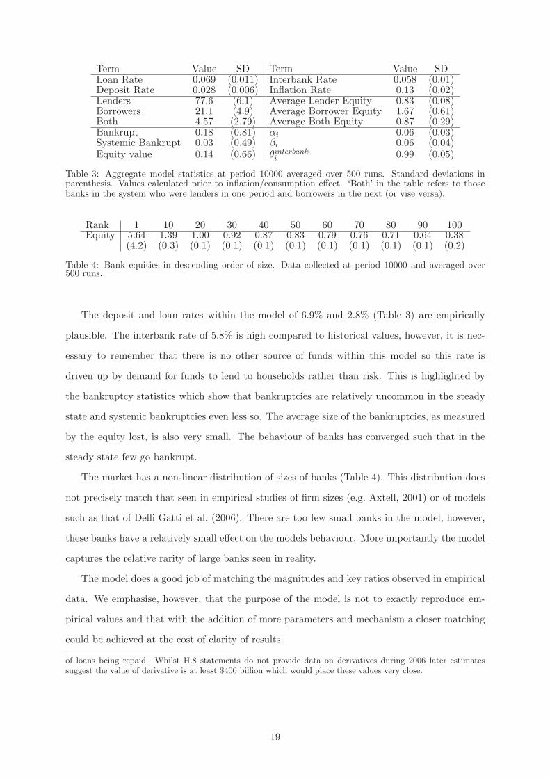
The deposit and loan rates within the model of 6.9% and 2.8% (Table 3) are empirically

plausible. The interbank rate of 5.8% is high compared to historical values, however, it is nec-

essary to remember that there is no other source of funds within this model so this rate is

driven up by demand for funds to lend to households rather than risk. This is highlighted by

the bankruptcy statistics which show that bankruptcies are relatively uncommon in the steady

state and systemic bankruptcies even less so. The average size of the bankruptcies, as measured

by the equity lost, is also very small. The behaviour of banks has converged such that in the

steady state few go bankrupt.

The market has a non-linear distribution of sizes of banks (Table 4). This distribution does

not precisely match that seen in empirical studies of firm sizes (e.g. Axtell, 2001) or of models

such as that of Delli Gatti et al. (2006). There are too few small banks in the model, however,

these banks have a relatively small effect on the models behaviour. More importantly the model

captures the relative rarity of large banks seen in reality.

The model does a good job of matching the magnitudes and key ratios observed in empirical

data. We emphasise, however, that the purpose of the model is not to exactly reproduce em-

pirical values and that with the addition of more parameters and mechanism a closer matching

could be achieved at the cost of clarity of results.

of loans being repaid. Whilst H.8 statements do not provide data on derivatives during 2006 later estimatessuggest the value of derivative is at least $400 billion which would place these values very close.

19

Large Large Smallλ Connections Component Largest to to to

Component Large Small Small0.0 180.0 12.0 24.1 65.4 97.5 17.1

(26.7) (3.1) (10.3) (9.4) (21.2) (13.2)0.1 386.5 6.9 40.7 123.3 210.4 52.7

(55.0) (1.5) (10.5) (13.8) (44.6) (29.1)0.2 684.2 4.3 58.7 207.2 364.3 112.7

(109.4) (0.9) (10.8) (26.2) (89.3) (57.6)0.3 1017.7 2.9 70.3 307.8 537.2 172.7

(154.2) (0.8) (8.7) (39.6) (124.8) (81.5)0.4 1307.4 1.9 77.5 408.9 694.5 204.0

(204.0) (0.7) (6.2) (56.8) (165.7) (104.6)0.5 1643.0 1.5 79.8 517.4 875.5 250.1

(253.3) (0.6) (5.0) (69.9) (205.6) (130.5)0.6 1965.0 1.2 80.9 627.4 1054.7 282.9

(298.9) (0.4) (5.0) (83.1) (244.0) (151.3)0.7 2298.5 1.1 81.4 727.2 1227.1 344.2

(339.4) (0.2) (4.5) (95.1) (272.5) (178.5)0.8 2598.6 1.0 81.7 829.6 1391.5 377.4

(394.2) (0.1) (5.0) (111.2) (314.7) (209.7)0.9 2984.0 1.0 80.9 942.2 1597.3 444.6

(440.6) (0.0) (5.0) (123.0) (359.6) (222.9)1.0 3298.9 1.0 81.6 1049.1 1778.5 471.2

(494.8) (0.0) (5.0) (137.4) (403.6) (251.2)

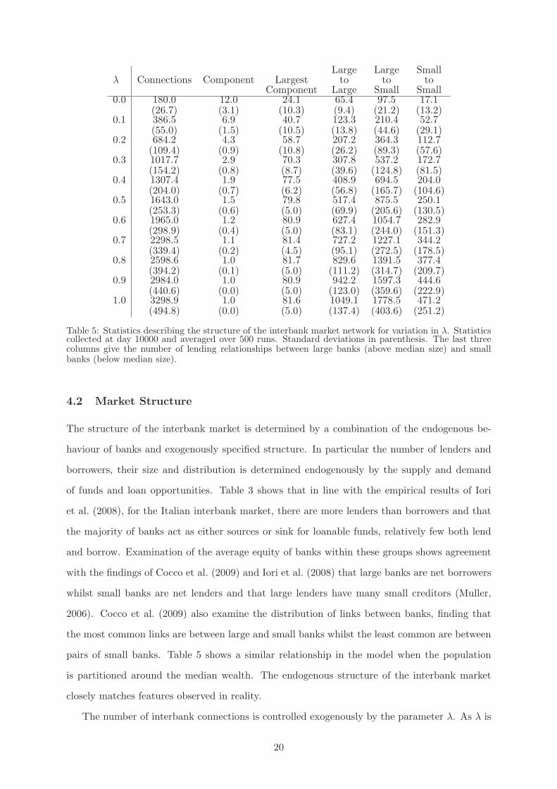
Table 5: Statistics describing the structure of the interbank market network for variation in λ. Statisticscollected at day 10000 and averaged over 500 runs. Standard deviations in parenthesis. The last threecolumns give the number of lending relationships between large banks (above median size) and smallbanks (below median size).

4.2 Market Structure

The structure of the interbank market is determined by a combination of the endogenous be-

haviour of banks and exogenously specified structure. In particular the number of lenders and

borrowers, their size and distribution is determined endogenously by the supply and demand

of funds and loan opportunities. Table 3 shows that in line with the empirical results of Iori

et al. (2008), for the Italian interbank market, there are more lenders than borrowers and that

the majority of banks act as either sources or sink for loanable funds, relatively few both lend

and borrow. Examination of the average equity of banks within these groups shows agreement

with the findings of Cocco et al. (2009) and Iori et al. (2008) that large banks are net borrowers

whilst small banks are net lenders and that large lenders have many small creditors (Muller,

2006). Cocco et al. (2009) also examine the distribution of links between banks, finding that

the most common links are between large and small banks whilst the least common are between

pairs of small banks. Table 5 shows a similar relationship in the model when the population

is partitioned around the median wealth. The endogenous structure of the interbank market

closely matches features observed in reality.

The number of interbank connections is controlled exogenously by the parameter λ. As λ is

20

increased Table 5 shows that the number of interbank connections increases in direct proportion.

For λ = 0, given the numbers of lenders and borrowers the market is close to being minimally

connected15. Whilst for λ = 1 the market is much more densely connected, for any given time

step, all borrowers are connected to all lenders. Table 5 also shows the number of components

into which the interbank network is split. A component is a set of vertices which are all connected

through paths but are not connected to any nodes outside of the set. Here we calculate compo-

nents based on the directed graph, considering i connected to j only if i lent funds to j. Each

component therefore represents the maximum extent of contagion from a single bankruptcy. For

values of λ > 0.5 there is on average only one component. This means that there exists at least

one bank, who’s failure could theoretically effect every other bank within the market. For lower

values of λ this is not the case, the maximum impact of any failure is restricted.

4.3 Individual Bankruptcy

Opinion is divided on the effect of the structure of the interbank market on the probability and

severity of contagion. Two opposing roles have been identified: Allen and Gale (2001) highlight

the stabilising quality, arguing that the more connected a market is the more efficiently risk

is shared and the effect of a shock mitigating. In contrast Vivier-Lirimont (2006) and others

argue that the more connected an interbank market is, the more banks will be involved in failure

cascades and the faster these cascades will spread. In order to identify these effects within this

model we first consider the bankruptcy of a single bank and its impact on the financial system.

A similar analysis has been conducted in a number of studies both analytically and empirically

for a range of interbank markets16. In each case the authors examine how a shock centred on

a single bank or region affects the remainder of the financial system, potentially causing the

collapse of multiple banks in a cascade.

In an analysis using Austrian data, Elsinger et al. (2006) show that systemic failures from

the collapse of a single bank only occur in about 1% of cases of bank defaults. Further, only a

small proportion of banks are able to cause systemic crisis were they to fail (Boss et al., 2004)

and similarly only a small proportion of banks are themselves susceptible to the bankruptcy of

15The minimally connected market would consist of each lender being connected to a single borrower meaningover two periods the minimum number of interbank connections is approximately equal to double the numberof lenders. For λ = 1 each lender is connected to each borrower within a particular time step. The number ofconnections is close to lenders× borrowers, remembering that the exact number of lenders and borrowers varieseach time step.

16For example: Boss et al. (2004), Upper and Worms (2004), Nier et al. (2007), Gai and Kapadia (2010)Vivier-Lirimont (2006) and Allen and Gale (2001).

21

λ Contagion Probability Size Equity Cause Equity Largest0 1.62 0.226 7.16 5.45 2.08 19.8

(0.61) (0.059) (3.98) (1.80) (3.20) (10.5)0.1 1.59 0.213 7.45 5.93 1.84 24.6

(0.45) (0.049) (2.87) (1.66) (1.15) (11.7)0.2 1.43 0.183 7.82 6.16 1.92 28.9

(0.47) (0.036) (3.30) (2.07) (0.83) (13.1)0.3 1.17 0.144 8.10 6.23 2.15 28.8

(0.52) (0.029) (3.90) (2.55) (0.90) (14.3)0.4 0.96 0.105 9.15 6.92 2.52 29.8

(0.60) (0.029) (4.88) (3.32) (1.05) (16.5)0.5 0.71 0.074 9.58 7.23 2.81 27.5

(0.75) (0.030) (6.06) (4.32) (1.06) (18.1)0.6 0.57 0.052 10.89 8.13 3.15 27.2

(0.93) (0.029) (8.06) (5.91) (1.31) (20.3)0.7 0.43 0.036 11.75 8.77 3.28 25.8

(1.18) (0.026) (10.90) (8.19) (1.74) (23.30)0.8 0.35 0.026 13.46 9.98 3.34 26.0

(1.42) (0.024) (14.56) (10.88) (2.29) (26.5)0.9 0.26 0.018 13.93 10.19 3.24 23.4

(1.77) (0.022) (18.42) (13.85) (2.94) (28.7)1 0.22 0.013 16.79 12.24 3.13 23.1

(2.10) (0.019) (25.70) (19.14) (3.51) (32.4)

Table 6: Statistics showing the effects of single bankruptcies on the economy for variation in λ. Contagionis the average number of banks which fail as a consequence of a single bank being made bankrupt(excluding the initial bank). Probability is the chance that contagion will occur. Size is the averagenumber of banks which go bankrupt conditional on contagion occurring whilst equity is the value of thesebanks. Cause Equity is the average equity of the banks which cause contagion. Largest is the size of thelargest contagion. Data collected using market states saved at period 10000 and averaged over 500 runs.

a partner institution (Angelini et al., 1996). The effect of contagion when it occurs, however,

can be very large (Gai and Kapadia, 2010). Humphrey (1986) shows that the collapse of a large

American bank could potentially bankrupt 37% of banks in the market.

The converged economies presented in the previous section serve as a basis for this analysis.

The state of the market is saved and a single bank is made bankrupt by setting its equity and

reserves to zero. The effect of this bankruptcy on the rest of the economy is recorded before the

state of the market is reset to the saved state. This is repeated for each bank in turn until the

failure of all banks have been considered.

Table 6 shows the impact of a single bankruptcy on the rest of the market. There is a clear

relationship, as the market becomes more connected the effect of the bankruptcy decreases. This

supports the findings of Allen and Gale (2001), Giesecke and Weber (2006) and Freixas et al.

(2000). The mechanism behind this relationship deserves further attention. Table 6 displays

the probability of contagion; that the collapse of any given bank will induce at least one other

bank to collapse. The decreasing probability as markets become more connected agrees with

the relationship demonstrated by Brusco and Castiglionesi (2007); whilst more banks may be

touched by contagion, if the market is more connected the probability that any of them will fail

22

is reduced. Empirically, Angelini et al. (1996) and Boss et al. (2004) in their analysis of the

Italian and Austrian interbank markets both find the probability of a bank collapse causing a

systemic event to be approximately 4% which corresponds to a market in the upper-middle of

the connectivity distribution.

The same table also shows the number of banks which go bankrupt conditional on there being

a contagious failure. As the market becomes more connected more banks fail in each contagious

event. This appears to suggest a greater vulnerability, however, this is not the case. The table

shows that the average equity of the banks which cause contagion increases with connectivity.

As the market becomes more connected only the larger banks with more borrowing are able to

cause contagious failures. The impact of smaller banks is sufficiently well spread that in many

cases they do not cause other banks to fail. The table also shows that the average equity of

failing banks is less than the market average of one, indicating that smaller banks are more

vulnerable to contagious failure.

An alternative measure of a market’s potential susceptibility to contagion is the maximum

number of bankruptcies a failure may cause. The sizes of the largest failures in the model are of

the same magnitude as those seen in reality. Upper and Worms (2004) find within the German

Banking system a single bankruptcy may cause at most 15% of the other banks to fail whilst

Humphrey (1986) shows that the collapse of a major US bank could lead to 37% of banks de-

faulting. The relationship with connectivity differs from that of average contagion. Here the

most vulnerable markets are those with an intermediate level of connectivity (λ = 0.4). Whilst

not, on average, the most susceptible to contagion these markets are particularly vulnerable to

the failure of crucial banks. Banks within these markets are sufficiently poorly connected that

if one fails, the shock is strong enough to drive other banks to failure. At the same time Table 5

shows that for λ = 0.4 in many cases the market only has a single component, meaning that

a single bankruptcy could effect the whole market. The combination of large shocks and wide

spread combine to make these markets particularly vulnerable if the wrong large bank fails.

The results in this section have shown that a more connected interbank market allows more

efficient risk sharing reducing the market’s overall susceptibility to contagion. They also high-

lighted a potential vulnerability of intermediately connected markets which, whilst not the most

susceptible to contagion do potentially suffer from the largest failure cascades.

23

4.4 Systemic Shocks

The results presented in the previous section describe how an individual bankruptcy can cause

contagion. These results are important in understanding the vulnerability of the financial sys-

tem to an isolated failure, however, in reality the failure of a bank is often not a spontaneous

event. Instead a failure may be caused by a shock which effects the whole financial system.

For instance, Gorton (1988) shows that bank panics are most common at the beginning of an

economy wide recession. Events such as this can affect multiple institutions simultaneously,

weakening balance sheets and potentially causing several unconnected banks to fail at the same

time. As a result there may be overlapping cascades of bankruptcies. This section will consider

the effect of such a macro-economic shock on the system.

Little attention has been given to the effect of the interbank market during a systemic shock.

It is unclear how the risk bearing and contagion spreading effects interact as equity is eroded.

A more connected market may allow system liquidity to be better utilised, spreading the effect

of the shock and so reducing the severity. Alternatively, as the market becomes more connected

the weakest banks may be more likely to be effected by bankruptcies causing more of them to

fail. One study which looks at this issue is that of Lorenz and Battiston (2008). They find that

increasing interbank market connectivity at first reduces the incidence of bankruptcy but for

more connected markets it increases. This model, however, does not permit cascades of failures,

a key mechanism in the spread of contagion. Whilst not explicitly modelling a systemic shock,

Battiston et al. (2009) permit multiple bankruptcies to occur in the same period. They find

a similar pattern to Lorenz and Battiston (2008) but in this case attribute it to the financial

accelerator, a positive feedback mechanism by which the deterioration of a bank’s financial posi-

tion may cause further deterioration in future time periods. As connectivity within the market

increases, the accelerator effect dominates the risk spreading effect leading to an amplification of

shocks to individual banks and consequently increased bankruptcies. There is no analogous ef-

fect within this model. Without the financial accelerator the authors show the same relationship

as seen in this model for small shocks i.e. increasing connectivity decreases bankruptcies.

In addition it is not clear whether contagion in the interbank market will be significant or

if it will be secondary to the financial shock itself. Giesecke and Weber (2006) find that conta-

gion is a second order effect compared to portfolio losses. If this is the case, within our model

it would be expected that the number of failures due to the macro-economic shock would be

greater than that caused by contagion. In contrast, Elsinger et al. (2006) show that whilst the

24

0 0.5 10

5θshock=0.95

λB

ankr

upt

0 0.5 10

5

10

15θshock=0.9

λ

Ban

krup

t

0 0.5 110

20

30θshock=0.85

λ

Ban

krup

t

0 0.5 120

30

40

50θshock=0.8

λ

Ban

krup

t

0 0.5 130

40

50

60θshock=0.775

λ

Ban

krup

t

0 0.5 140

50

60

70θshock=0.75

λ

Ban

krup

t

0 0.5 140

60

80θshock=0.7

λ

Ban

krup

t

0 0.5 1

60

80

θshock=0.65

λ

Ban

krup

t

0 0.5 1

60

80

100θshock=0.6

λ

Ban

krup

t

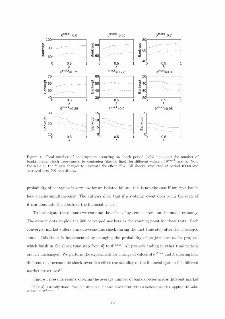
Figure 1: Total number of bankruptcies occurring on shock period (solid line) and the number ofbankruptcies which were caused by contagion (dashed line), for different values of θshock and λ. Notethe scale on the Y axis changes to illustrate the effect of λ. All shocks conducted at period 10000 andaveraged over 500 repetitions.

probability of contagion is very low for an isolated failure, this is not the case if multiple banks

face a crisis simultaneously. The authors show that if a systemic event does occur the scale of

it can dominate the effects of the financial shock.

To investigate these issues we examine the effect of systemic shocks on the model economy.

The experiments employ the 500 converged markets as the starting point for these tests. Each

converged market suffers a macro-economic shock during the first time step after the converged

state. This shock is implemented by changing the probability of project success for projects

which finish in the shock time step from θti to θshock. All projects ending in other time periods

are left unchanged. We perform the experiment for a range of values of θshock and λ showing how

different macroeconomic shock severities effect the stability of the financial system for different

market structures17.

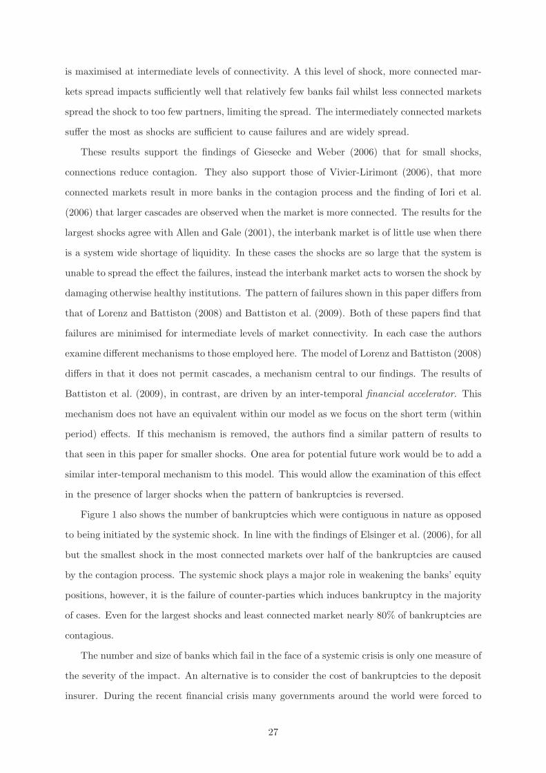
Figure 1 presents results showing the average number of bankruptcies across different market

17Note θti is usually drawn from a distribution for each investment, when a systemic shock is applied the value

is fixed at θshock.

25

architectures and for different shock severity’s. As θshock decreases fewer projects are completed

successfully. This leads to higher losses for banks and consequently more failures. Market con-

nectivity, however, has a non-linear effect on this relationship. For small shocks a more highly

connected market reduces bankruptcies, limiting the spread of contagion by spreading the im-

pact of failures. In contrast for larger shocks the pattern is revered, more sparsely connected

markets are less susceptible to contagion. The point at which the effect of the market changes

is approximately θshock = 0.775. For shocks of this size the most fragile market structure is

an intermediately connected market. Here both the contagion spreading and risk spreading ef-

fects are in evidence and of a similar magnitude. As market connectivity increases the contagion

spreading effect leads to an increase in bankruptcies. For λ > 0.5, however, the impact spreading

effect of contagion becomes dominant leading to a reduction in bankruptcies.

The results show that the structure of the interbank market influences the size of the conta-

gious event. The extent of contagion is highly dependent on the degree to which failures spread.

This is governed by two effects both of which vary with market connectivity: the number of

banks to which each bank is connected and the probability that the interbank loan between two

banks is larger than the lender’s equity. As connectivity increases each bankruptcy affects more

counter-parties. At the same time lender’s split the same amount of funds between more banks

meaning the probability that an interbank loan is greater than the partner’s equity, therefore

causing bankruptcy if not repaid, is reduced.

A systemic shock reduces the equity of all banks. For small shocks, in highly connected mar-

kets, banks are sufficiently well capitalised and the effect of the shock sufficiently well spread

that the failure of a bank rarely has sufficient impact to cause a counter-party to fail. As con-

nectivity decreases the average loan size to counter-parties increases and so contagious failures

becomes more likely. Larger systemic shocks result in reduced bank equities and so smaller

losses from interbank loans may cause failures. Consequently banks in more connected markets

will start to be at risk from the failure of their counter-parties. For the largest systemic shocks

bank equities are damaged to such an extent that regardless of connectivity the size of interbank

loans are sufficient to cause them to fail. Instead of spreading the impact so it may be absorbed,

the higher connectivity results in more banks being effected and failing. In less well-connected

markets banks still fail though the scope of contagion is reduced as each bank failure effects a

smaller subset of the population.

For θshock = 0.775 the point at which the liklihood of a bank failing and spreading a shock

26

is maximised at intermediate levels of connectivity. A this level of shock, more connected mar-

kets spread impacts sufficiently well that relatively few banks fail whilst less connected markets

spread the shock to too few partners, limiting the spread. The intermediately connected markets

suffer the most as shocks are sufficient to cause failures and are widely spread.

These results support the findings of Giesecke and Weber (2006) that for small shocks,

connections reduce contagion. They also support those of Vivier-Lirimont (2006), that more

connected markets result in more banks in the contagion process and the finding of Iori et al.

(2006) that larger cascades are observed when the market is more connected. The results for the

largest shocks agree with Allen and Gale (2001), the interbank market is of little use when there

is a system wide shortage of liquidity. In these cases the shocks are so large that the system is

unable to spread the effect the failures, instead the interbank market acts to worsen the shock by

damaging otherwise healthy institutions. The pattern of failures shown in this paper differs from

that of Lorenz and Battiston (2008) and Battiston et al. (2009). Both of these papers find that

failures are minimised for intermediate levels of market connectivity. In each case the authors

examine different mechanisms to those employed here. The model of Lorenz and Battiston (2008)

differs in that it does not permit cascades, a mechanism central to our findings. The results of

Battiston et al. (2009), in contrast, are driven by an inter-temporal financial accelerator. This

mechanism does not have an equivalent within our model as we focus on the short term (within

period) effects. If this mechanism is removed, the authors find a similar pattern of results to

that seen in this paper for smaller shocks. One area for potential future work would be to add a

similar inter-temporal mechanism to this model. This would allow the examination of this effect

in the presence of larger shocks when the pattern of bankruptcies is reversed.

Figure 1 also shows the number of bankruptcies which were contiguous in nature as opposed

to being initiated by the systemic shock. In line with the findings of Elsinger et al. (2006), for all

but the smallest shock in the most connected markets over half of the bankruptcies are caused

by the contagion process. The systemic shock plays a major role in weakening the banks’ equity

positions, however, it is the failure of counter-parties which induces bankruptcy in the majority

of cases. Even for the largest shocks and least connected market nearly 80% of bankruptcies are

contagious.

The number and size of banks which fail in the face of a systemic crisis is only one measure of

the severity of the impact. An alternative is to consider the cost of bankruptcies to the deposit

insurer. During the recent financial crisis many governments around the world were forced to

27

0 0.1 0.2 0.3 0.4 0.5 0.6 0.7 0.8 0.9 10

10

20

30

40

50

60

70

80

90

100

λ

Cos

t

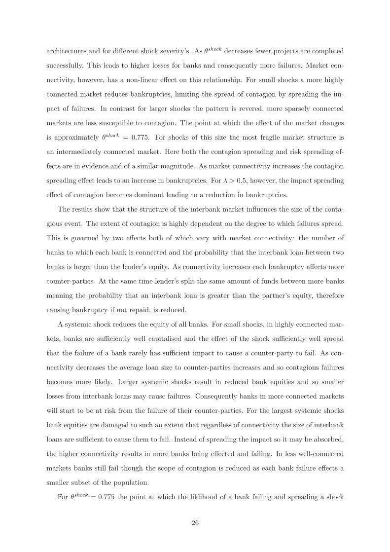
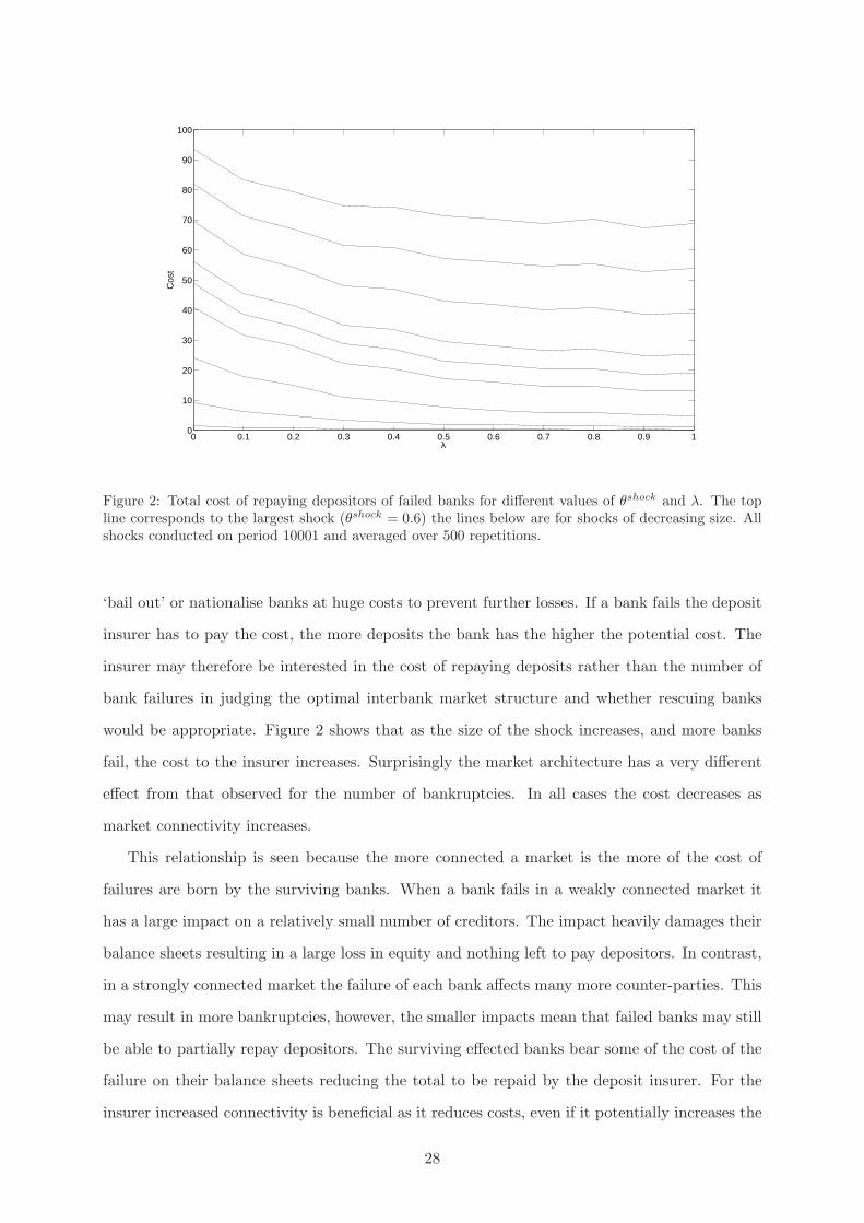
Figure 2: Total cost of repaying depositors of failed banks for different values of θshock and λ. The topline corresponds to the largest shock (θshock = 0.6) the lines below are for shocks of decreasing size. Allshocks conducted on period 10001 and averaged over 500 repetitions.

‘bail out’ or nationalise banks at huge costs to prevent further losses. If a bank fails the deposit

insurer has to pay the cost, the more deposits the bank has the higher the potential cost. The

insurer may therefore be interested in the cost of repaying deposits rather than the number of

bank failures in judging the optimal interbank market structure and whether rescuing banks

would be appropriate. Figure 2 shows that as the size of the shock increases, and more banks

fail, the cost to the insurer increases. Surprisingly the market architecture has a very different

effect from that observed for the number of bankruptcies. In all cases the cost decreases as

market connectivity increases.

This relationship is seen because the more connected a market is the more of the cost of

failures are born by the surviving banks. When a bank fails in a weakly connected market it

has a large impact on a relatively small number of creditors. The impact heavily damages their

balance sheets resulting in a large loss in equity and nothing left to pay depositors. In contrast,

in a strongly connected market the failure of each bank affects many more counter-parties. This

may result in more bankruptcies, however, the smaller impacts mean that failed banks may still

be able to partially repay depositors. The surviving effected banks bear some of the cost of the

failure on their balance sheets reducing the total to be repaid by the deposit insurer. For the

insurer increased connectivity is beneficial as it reduces costs, even if it potentially increases the

28

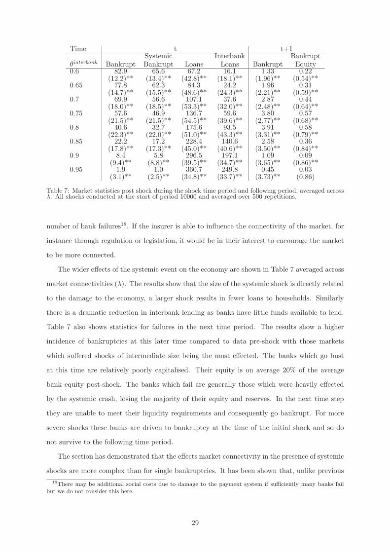
Time t t+1Systemic Interbank Bankrupt

θinterbank Bankrupt Bankrupt Loans Loans Bankrupt Equity0.6 82.9 65.6 67.2 16.1 1.33 0.22

(12.2)** (13.4)** (42.8)** (18.1)** (1.96)** (0.54)**0.65 77.8 62.3 84.3 24.2 1.96 0.31

(14.7)** (15.5)** (48.6)** (24.3)** (2.21)** (0.59)**0.7 69.9 56.6 107.1 37.6 2.87 0.44

(18.0)** (18.5)** (53.3)** (32.0)** (2.48)** (0.64)**0.75 57.6 46.9 136.7 59.6 3.80 0.57

(21.5)** (21.5)** (54.5)** (39.6)** (2.77)** (0.68)**0.8 40.6 32.7 175.6 93.5 3.91 0.58

(22.3)** (22.0)** (51.0)** (43.3)** (3.31)** (0.79)**0.85 22.2 17.2 228.4 140.6 2.58 0.36

(17.8)** (17.3)** (45.0)** (40.6)** (3.50)** (0.84)**0.9 8.4 5.8 296.5 197.1 1.09 0.09

(9.4)** (8.8)** (39.5)** (34.7)** (3.65)** (0.86)**0.95 1.9 1.0 360.7 249.8 0.45 0.03

(3.1)** (2.5)** (34.8)** (33.7)** (3.73)** (0.86)

Table 7: Market statistics post shock during the shock time period and following period, averaged acrossλ. All shocks conducted at the start of period 10000 and averaged over 500 repetitions.

number of bank failures18. If the insurer is able to influence the connectivity of the market, for

instance through regulation or legislation, it would be in their interest to encourage the market

to be more connected.

The wider effects of the systemic event on the economy are shown in Table 7 averaged across

market connectivities (λ). The results show that the size of the systemic shock is directly related

to the damage to the economy, a larger shock results in fewer loans to households. Similarly

there is a dramatic reduction in interbank lending as banks have little funds available to lend.

Table 7 also shows statistics for failures in the next time period. The results show a higher

incidence of bankruptcies at this later time compared to data pre-shock with those markets

which suffered shocks of intermediate size being the most effected. The banks which go bust

at this time are relatively poorly capitalised. Their equity is on average 20% of the average

bank equity post-shock. The banks which fail are generally those which were heavily effected

by the systemic crash, losing the majority of their equity and reserves. In the next time step

they are unable to meet their liquidity requirements and consequently go bankrupt. For more

severe shocks these banks are driven to bankruptcy at the time of the initial shock and so do

not survive to the following time period.

The section has demonstrated that the effects market connectivity in the presence of systemic

shocks are more complex than for single bankruptcies. It has been shown that, unlike previous

18There may be additional social costs due to damage to the payment system if sufficiently many banks failbut we do not consider this here.

29

studies, there is no optimal level of market connectivity to minimise the impact of a systemic

crisis. Connectivity may exacerbate or dampen the effect depending on the shock severity. For

deposit insurers, however, there is an optimum structure as more connected markets minimise

the cost of repaying deposits.

5 Regulation

The previous section highlighted the effects of the market structure on contagion under both

individual and systemic shocks. Here we will consider mechanisms for limiting the impact of

these events and their wider effect on the market state.

5.1 Equity and Reserve ratio

A key proposal put forward in the Basel III reforms requires banks to hold a higher percentage

of capital relative to their risky assets. As a result , banks are more tightly constrained in the

degree to which they can leverage their positions and so should be less at risk of failure through

poor investment outcomes. An alternative proposal has been made to tighten banks minimum

reserve ratios. This change would force banks to hold a higher proportion of liquid reserves

which would provide them with increased protection against liquidity shocks. Both of these

mechanism are tested within this model. The equity and reserve ratios are varied independently

and 500 further experiments conducted for each parameter combination. We consider increases

of each requirement by 50%. We focus our analysis on the case of systemic shocks as the effect

of these changes on individual failures has already received much attention. For instance Nier

et al. (2007), Iori et al. (2006) and Gai and Kapadia (2010) all find that increasing the amount

of reserves which banks hold reduces the number of bankruptcies.

Figure 3 shows the effect of the regulatory changes on the probability of contagious bankrupt-

cies. Increasing the equity ratio results in a large reduction in failures in nearly all cases. The

reduced level of leverage reduces the level of the macro-economic shock. At the same time there is

a reduction in interbank lending which limits the impact of failing banks on their counter-parties.

Together these two factors combine to reduce the total effect of the shock. Increasing the reserve

ratio has relatively little effect on the market susceptibility to contagion. For large shocks there

is a small reduction in the number of bankruptcies whilst for small shocks there is no significant

difference. The reason for this is that the contagion process is primarily driven by banks failing

30

0 0.5 10

1

2

3θshock=0.95

λB

ankr

upt

0 0.5 10

10

20θshock=0.9

λ

Ban

krup

t

0 0.5 10

10

20

30θshock=0.85

λ

Ban

krup

t

0 0.5 10

50

θshock=0.8

λ

Ban

krup

t

0 0.5 10

50

θshock=0.775

λ

Ban

krup

t

0 0.5 10

50

θshock=0.75

λ

Ban

krup

t

0 0.5 10

50

θshock=0.7

λ

Ban

krup

t

0 0.5 10

50

100θshock=0.65

λ

Ban

krup

t

0 0.5 10

50

100θshock=0.6

λ

Ban

krup

t

Figure 3: Total number of bankruptcies occurring on shock period for the base model (solid line),increased equity ratio (dashed line) and increased reserve ratio (dotted line), for different values of θshock

and λ. Note the changing scale on the Y axis to illustrate changes with λ. All shocks conducted atperiod 10000 and averaged over 500 repetitions in each case.

through lack of equity. The increased reserve ratio means banks hold more liquid funds which

may allow a bank to repay a loan when one of its own loans is not repaid. This effect is more ben-

eficial when interbank loans are small so that if they are not repaid the shortfall may be covered

by the additional liquid reserves. In the model market, as in real markets, there are relatively

few banks which both lend and borrow (Iori et al., 2008) so increasing liquidity has a limited ef-

fect. Whilst both of the regulations reduce the number of bankruptcies the mechanism by which

they do so, restricted lending to households and banks, has a negative effect on the economy as

a whole. The average value of loans to households reduces by 8% to 361.3 for the change in re-

serve ratio and 12% to 345.1 for the change in equity ratio. The overall effect of these regulatory

changes is therefore ambiguous, they reduce bankruptcies but at the same time reduce lending.

31

ηShock Size ∞ 10 5 2

0.6 82.9 82.5 66.1 37.1(12.17) (12.49) (15.48)** (13.51)**

0.65 77.8 77.5 59.4 31.7(14.67) (14.88) (16.59)** (12.32)**

0.7 69.9 69.7 50.5 26.3(18.03) (18.12) (17.39)** (10.57)**

0.75 57.6 57.6 39.0 21.6(21.46) (21.44) (17.01)** (8.92)**

0.8 40.6 40.6 26.1 17.4(22.43) (22.40) (15.95)** (8.10)**

0.85 22.2 22.3 15.1 13.3(17.76) (17.75) (9.43)** (5.89)**

0.9 8.4 8.4 7.8 9.4(9.37) (9.35) (5.41)** (4.55)**

0.95 1.9 2.0 3.3 5.4(3.07) (3.22) (3.08)** (3.02)**

Loans 391.5 392.9 404.0 303.3(32.62) (35.44) (75.58)** (86.72)**

Interbank Loans 283.3 282.2 189.3 66.1(36.91) (39.98) (63.64)** (27.25)**

Lending Rate 0.069 0.068 0.050 0.025(0.008) (0.006) (0.008)** (0.001)**

Interbank Rate 0.058 0.058 0.045 0.016(0.010) (0.013) (0.018)** (0.011)**

Table 8: Statistics showing the effects of systemic shocks on the economy for different borrowingconstraints averaged across λ. All shocks conducted at period 10000 and averaged over 500 repetitionsin each case. η = ∞ corresponds to the base case where there is no constraint. The market statistics atthe bottom are pre-crash values.

5.2 Borrowing Constraints

An alternatively to constraining the total lending or borrowing is to instead constrain the max-

imum funds a bank may lend to a single counter-party. This approach forces banks to diversify

their interbank lending, making them less susceptible to the failure of a single debtor. Here we

implement this regulation by limiting the maximum a particular lender may lend to a particular

borrower to be a multiple η of the borrowers equity. As a consequence larger banks with more

equity may borrow more from any given lender.

Table 8 presents the results of 500 simulation for three different borrowing constraints. For

η = 10 it can be seen that the constraint does not effect the results, there is no significant change

in any of the market statistics. As η is decreased the constraint becomes binding. For η = 5 the

effect of the regulation is beneficial, the number of systemic bankruptcies is significantly reduced

in all but one case. The regulatory change limits the size of the interbank connections reducing

the probability of a bank failing due to the collapse of one of its creditors. The regulatory

change also has a broader beneficial effect. There is a reduction in the demand for interbank

loans which, reduces the total volume of loans and the interest rate in this market. As a result

32

the volume of loans to households increases and there is more competition between banks forcing

down the household borrowing rate.

Care, however, must be taken with the implementation of this regulation. If the borrowing

constraints are too tight there can be substantial negative effects. For η = 2 there is still a sig-

nificant reduction in bankruptcies. The function of the interbank market, however, is severely

impaired, meaning funds are no longer efficiently allocated and the total value of loans to house-

holds is heavily reduced. By regulating too heavily the economy is severely restricted.

6 Model Sensitivity

This section presents results detailing the robustness of the model to changes in parameters and

specification. The initial model presented above provides a relatively simple framework which

captures the key behaviours of banks and households. Assumptions were made in forming the

model, which whilst making it more transparent, over simplified important aspects of real world

behaviour. Here we relax several of these assumptions which move the model closer to reality

whilst also permitting a greater degree of heterogeneity within the system. By comparing the

modified model behaviour to the base case we are able to determine the effect of the changes

in a clear manner, which would not have been possible if they had been included in the initial

model formation.

6.1 Parameter sensitivity

The results presented above are based on one parameter combination. In order to fully under-

stand the model it is important to determine the robustness of the results and how behaviour

changes if parameters are varied. Table 1 details the models six key parameters. Of these six,

changes to αg and βg have already been considered as regulatory actions. Here we will consider

the remaining four.

Varying the payoff from investments, µ, effects the loan, deposit and interbank interest rates.

Greater returns from investments allow banks to charge households higher interest rates which

in turn allows banks to pay higher rates for funds from both depositors and on the interbank

market. The model is robust to a wide range of values. µ = 1.15 was chosen as it produced

deposit and loans rates comparable to reality.

The parameters controlling the probability of a successful investment, θ, and the number

33

Interbank Confidence Credit WorthinessBankrupt 0.258 (1.113) 0.04 (0.26)**Systemic Bankrupt 0.045 (0.662) 0.002 (0.06)**Loans 341.04 (89.2)** 410.65 (20.32)**I-B Loans 246.64 (80.42)** 247.65 (28.77)**I-B Rate 0.155 (0.379)** 0.054 (0.008)**Loan Rate 0.065 (0.009)** 0.066 (0.008)**Deposit Rate 0.026 (0.005)** 0.027 (0.006)**θinterbank 0.97 (0.08) 0.99 (0.004)**Reaction 0.47 (0.28) - -

Table 9: Steady state market statistics for two model variations. Values consistent over λ, calculated intime period 10000 and averaged over 500 repetitions in each case.

of households, M , are closely linked. Together they control the supply of potentially fundable

loan requests. A decrease in households results in fewer loan requests per time-period, whilst a

decrease in θ reduces the expected return of projects making fewer profitably fundable19. The

results of the model are robust across a wide range of parameter values (0.9 < θ < 0.999,

M > 20N), if either or both values are too low there may be insufficient profitable investment

proposals resulting in unallocated funds and potentially no interbank lending. M = 10000 and

θ = 0.99 was chosen for computational reasons whilst providing sufficient supply of funding re-

quest. Increasing M beyond this point leads to significantly slower program execution without

changing the results.

While θ and M describe the supply of investment projects, N , the number of banks, con-

trols the demand. The model produces qualitatively similar results for a wide range of values

(N > 40). N = 100 was chosen as it is of the same magnitude as the number of banks in many

of the worlds interbank markets (though some are much larger or smaller)20.

6.2 Interbank confidence

One of the key features of the recent financial crisis was the loss of liquidity within interbank

markets. Banks observed the failures of other financial institutions and became reluctant to

lend due to the fear of not regaining their funds. The loss of confidence resulted in a shortage of

liquidity and an exacerbation of the crisis. In the model presented above the failure of a bank

may cause other banks to fail both in the current and future time periods (Table 7). Banks,

however, do not take this into account, they do not become more reluctant to lend even though

the probability of funds not being returned is increased. A parallel may be drawn here with

19Note this parameter also interacts with µ. The larger the value of µ the lower θ may be whilst maintaininga profitable project.

20Tables of results demonstrating the above relations are available from the author upon request.

34

Interbank Confidence Credit WorthinessShock Max Size Shock Max Size

0 1.39 (0.51)** 20.52 (10.20) 1.30 (0.71)** 21.85 (10.74)**0.1 1.34 (0.64)** 28.98 (14.07)** 1.39 (0.50)** 25.43 (11.68)0.2 1.28 (0.61)** 31.00 (15.42)* 1.19 (0.51)** 23.98 (12.74)**0.3 1.10 (0.59) 30.59 (14.86) 0.78 (0.63)** 22.30 (14.66)**0.4 1.00 (0.60) 34.39 (17.41)** 0.58 (0.71)** 22.76 (15.57)**0.5 0.84 (0.67)* 33.47 (18.61)** 0.44 (0.87)** 22.74 (17.49)**0.6 0.68 (0.82)* 32.46 (21.53)** 0.32 (1.04)** 20.81 (17.20)**0.7 0.67 (0.88)** 35.05 (22.64)** 0.26 (1.27)* 20.56 (18.76)**0.8 0.49 (1.14)* 32.29 (26.31)** 0.20 (1.55) 20.59 (22.06)*0.9 0.60 (1.15)** 39.55 (30.33)** 0.19 (1.79) 21.65 (25.61)1 0.57 (1.29)** 41.90 (35.11)** 0.16 (1.82) 23.16 (28.76)

Table 10: Statistics showing the effect of a single bankruptcy for different values of λ for two differentmodel cases. Results collected in time period 10000 and average over 500 repetitions in each case.

Interbank Confidence Credit WorthinessBankrupt Loans I-B Loans Bankrupt Loans I-B Loans

0.6 66.37 58.4 16.5 79.65 84.8 14.9(30.80)** (87.7) (55.8) (8.99)** (81.9)** (27.4)

0.65 62.43 69.2 20.0 73.77 109.3 24.0(30.60)** (93.5)* (57.4) (11.92)** (98.3)** (43.4)

0.7 56.79 83.9 25.9 64.74 141.1 40.7(30.10)** (102.0)** (61.6)* (15.86)** (112.0)** (64.9)

0.75 48.22 103.0 36.3 51.21 180.1 68.7(29.00)** (109.6)** (69.0)** (19.41)** (112.5)** (83.3)

0.8 35.46 126.8 53.7 33.71 227.8 109.4(26.00)** (109.5)** (75.6)** (19.32)** (91.9)** (80.9)*

0.85 20.07 156.4 79.0 17.20 285.6 158.5(19.50) (99.7)** (75.4)** (13.78)** (62.5)** (56.8)**

0.9 7.57 199.2 113.9 6.56 347.4 205.0(10.00) (93.9)** (77.6)** (6.27)** (37.7)** (35.6)**

0.95 1.79 267.6 171.3 1.70 392.2 235.0(3.30) (104.1)** (92.7)** (2.00) (24.4)** (29.7)**

Table 11: Statistics showing the effect of systemic shocks for two different model cases. Values averagedover λ, collected at period 10000 for 500 repetitions in each case.

the work of Lagunoff and Schreft (2001) who show that banks may change their portfolio of

investments to reduce their exposure to potential losses even if they have not directly suffered.

To capture this effect the model is modified. Equation 9 is changed such that:

f(Iti ) =

θinterbanki − κif

t, if Iti > 0

1, if Iti ≤ 0

(12)

Where f t is the number of banks which have failed in the current time step t and κi is a pa-

rameter controlling the size of bank i’s reaction to bankruptcies. A larger value of κi means that

bank i reacts more strongly to a bankruptcy with a greater loss of confidence in the interbank

market. The value of κi is assigned randomly at the start of the simulation and is optimised in

the same way as deposit and loan interest rates. f is set each time period based on the number

35

of bank failures.

Allowing banks to react to failures negatively effects the stability of the market. Table 9

shows that there are fewer loans to households and fewer interbank loans, both quantities also

have a higher standard deviation. The interbank interest rate in particular is very volatile. Dur-

ing some periods it is similar to the base case but in others, particularly after the failure of one

or more banks, it can be very high, essentially preventing interbank lending. The average size

of contagion in response to a single bankruptcy is similar to that of the base model (Table 10),

however, these is less variation with connectivity. Less connected markets are less vulnerable

whilst more connected markers are more so. This is because there is less interbank lending

between fewer banks. Consequently the magnitude of both the risk spreading and contagion

inducing effects are reduced making the effect of connectivity smaller. The effect of the more

volatile market may be seen in the size of the largest failures, these are in most case much

larger than the base model and increasing with connectivity. The sudden fluctuations in market

conditions can damage the positions of banks, amplifying the effect of an individual failure by

making counter-parties more likely to fail. The consequences of the reduction in lending may

also be seen in the reduction in bankruptcies due to systemic shocks (Table 11). Less interbank

lending means fewer banks fail due to contagion, however, this is accompanied by a much heavier

reduction in loans and interbank lending than seen in the base case. Banks react to the failure

of counter-parties by stopping lending on the interbank market. As a consequence funds are

less efficiently allocated and the economy as a whole suffers. Overall allowing banks to react

to information on bankruptcies is destabilising. It creates fluctuations in the supply of credit

between banks impairing the allocation of funds to households.

6.3 Credit Worthiness

In the base model it was assumed that there existed a single interbank interest rate. It was ar-

gued that this was a reasonable assumption if banks have limited information about each others

states, the probability of systemic events is low, and the market is efficient. In reality, however,

banks vary their interbank rates dependent on the counter-party. More credit worthy banks,

those thought less likely to fail, pay lower rates. At the same time banks tend to repeatedly

interact with the same counter-parties (Cocco et al., 2009) potentially allowing more attractive

interest rates due to improved information. A banks state and history effect the rate at which

it can lend and borrow. Here we integrate this observation.

36

Each time period each bank has associated with it a risk premia, ζi drawn from |N(0, 1/Ei)|

which is the market estimation of the necessary compensation to lenders for the risk of it fail-

ing. This is to some extent a simplification of a potentially very complex effect. In reality a

banks risk premia is dependent on its own situation and the risk attitudes of all other market

participants. This mechanism, however, uses the observation that larger banks are less likely

to fail (e.g. Section 4.3) and so should receive more favourable terms. This rate is added to

the interbank rate bank i pays when it borrows. If a bank lends money it lends at the base

interbank rate. The recipients premia is not included when determining lending preferences as

any additional value received over the base interbank rate is considered to be fair compensation

for the additional risk borne.

The addition of a risk premia reduces interbank lending, however, unlike allowing bank to

vary their confidence in the interbank market, it does so in a relatively stable manner. As a result

the market is less volatile and more funds are allocated to households, there are fewer bankrupt-

cies and interest rates are lower (Table 9). This is reinforced in the results for single bankruptcies,

Table 10 shows the size of the contagious event is in nearly all cases reduced (along with the size

of the maximum bankruptcy). The system as a whole is also more resilient, even in large crisis the

extent of lending to households is less heavily reduced (Table 11). These results are in-line with

the findings of Park (1991), who shows that historically the availability of solvency information

regarding individual banks reduces the severity of panics. Here the risk premia is conditional on

bank equity and so is equivalent to giving banks this information. The introduction of the risk

premia makes it relatively more expensive for smaller and potentially more vulnerable banks to

borrow. As a consequence interbank lending along with the potential for systemic risk are both

reduced making the market more stable and the allocation of funds to households more efficient.

6.4 Endogenous Network Connectivity

In the base model all lenders have the same, exogenously determined, probability of being con-

nected to borrowers. Consequently each bank splits its lending between on average the same

number of counter-parties. The results in the previous sections have demonstrated how varying

the connectivity effects the probability that the failure of a bank may cause other banks to fail.

In particular it has highlighted the trade off between increased risk sharing and increased spread

of contagion. If systemic crisis are thought to be very rare or small in magnitude then from a so-

cial planners view a more connected market may be optimal as it reduces the effect of individual

37

bankruptcies along with reducing the cost of repaying the depositors of defaulting banks. For

the banks, however, this structure may not be optimal as in a completely connected market all

lenders suffer when a borrower fails. They may prefer a smaller number of connections, i.e. to

take a greater risk in the interbank market in exchange for less frequent costs. We capture this

effect within the model by allowing banks to select their own connectivity. The parameter λ is re-

placed by λi which is unique to each bank. This parameter is initially assigned randomly and op-

timised using the same evolutionary process as bank interest rates and reserve and equity ratios.

The banks converge to an intermediate level of connectivity λi = 0.44 (St. Dev 0.12). The

banks do not find it beneficial to lend to the maximum number of counter-parties, reducing their

risk of receiving a large shock, as to do so results in paying a small cost for every bankruptcy.

Neither are the banks willing to expose themselves to very high losses from a single counter-

party. The fact that this parameter is endogenous has very little effect on the market statistics.

The susceptibility to individual and systemic failures is not significantly different to the values

seen for similar levels of exogenously imposed market connectivity.

7 Conclusion

This paper has considered a model of a closed economy in which banks lend money to households

to fund investment projects. Banks gain funds to do this from a mixture of household deposits

and other banks. Interbank lending is conducted through an over-the-counter market in which

lenders and borrowers directly interact and establish loan contracts. Demand and supply within

this market determines the interbank interest rate. The model is simulated to find an equilib-

rium. It is shown that the balance sheets of the model banks capture key ratios and quantities

observed in empirical data. The effect of the structure of the interbank market on the suscepti-

bility of banks to individual and systemic shocks was considered. It was found that for individual

shocks interbank connections share the impact of failures. Consequently the expected number of

failures decreases as the number of interbank connections increase. Despite this relationship it

is found that intermediately connected markets potentially suffer the largest contagious failures.

These markets share risk less well than those better connected yet are potentially susceptible to

the failure of a single bank spreading and effecting the whole market making them particularly

susceptible to the failure of the largest banks. For systemic shocks the relationship is more

complex. The optimal interbank market connectivity varies with shock size. Previous work has

38

shown two contradictory relationships, both an increasing and decreasing liklihood of failures

with increasing market connectivity. The model presented here demonstrates the conditions un-

der which each effect is dominant. For small shocks higher connectivity helps to resist contagion

but for larger shocks it has the opposite effect. As a consequence there is no single best market

architecture able to limit contagion from systemic shocks. There is, however, an optimal market

structure for reducing the costs of these shocks. The more connected a market is, the more the

costs of failures are internalised reducing the cost to an insurer.

In order to limit the effects of contagion several regulatory actions were examined. Changes

to both the reserve and equity ratios were considered but were found to have ambiguous results.

In both cases increasing the ratios resulted in a decreased size of contagion but also decreased

lending, though both effects are more marked for changes in the equity ratio. Loan constraints

that limit the amount a lender may lend to a particular borrower, were also considered. If the

constrains were too lax they had no effect, whilst if they were too tight they reduced bankruptcy

but heavily damaged the efficiency of the economy, reducing the amount of funds allocated to

household loans. For intermediate levels of regulation bankruptcies were reduced and more loans

given to households, suggesting this could be a promising mechanism for limiting systemic risk. It

was also shown that if banks react to the bankruptcies of their peers the economy is destabilised

and funds are allocated less efficiently. In contrast if banks condition their lending rates on the

size of their counter-parties this reduces risk and makes the market less susceptible to contagion.

The model is used to explore regulations and changes to bank behaviour, however, the model

is sufficiently general that it invites further extension. The architecture of the market consid-

ered in this paper was imposed exogenously, the banks had no choice with regards to who their

counter-parties were. A richer model would relax this constraint, allowing lenders to select and

decline potential borrowers and to offer different interest rates based on the counter-parties finan-

cial position. This would allow issues such as the characterisation of the optimal market structure

to be addressed. Even without making this endogenous there are other market structures which

could be investigated, for instance hierarchical networks as seen in the UK interbank market.

The regulatory changes considered in this paper were of a static nature, regulations were

changed and the model simulated to find the new equilibrium. This does not have to be the case.

There is scope to investigate the application of regulations dynamically, for instance changing

capital or reserve requirement or providing banks with additional liquidity at particular points

in time. The role of the central bank was also not considered, however, in reality this may be

39

significant. For instance Allen et al. (2009) have shown how a central bank may limit volatil-

ity through open market operations. Central bank intervention, in the form of bail outs or

quantitative easing could be considered and the optimal structure and size determined.

The model also invites the addition of other financial products, in particular the addition

of credit default swap (CDS) contracts. Currently, lenders have no opportunity to protect

themselves against the default of their borrowers, CDS contracts would provide them with a

mechanism to do so. It is unclear what the effect of CDS contracts is on economic stability.

These instruments protect individual borrowers against the default of counter-parties, poten-

tially reducing the spread of contagion. At the same time, however, they open up new risks, if

a CDS provider defaults it takes with it the CDS contracts it was holding and so creates new

channels for loss within the system. The model may provide a test bed to investigate these issues.

References

Allen, F., Carletti, E., 2006. Credit risk transfer and contagion. Journal of Monetary Economics 53 (1),

89–111.

Allen, F., Carletti, E., Gale, D., 2009. Interbank market liquidity and central bank intervention. Journal

of Monetary Economics 56 (5), 639–652.

Allen, F., Gale, D., 2001. Financial contagion. Journal of Political Economy 108 (1), 1–33.

Angelini, P., Maresca, G., Russo, D., 1996. Systemic risk in the netting system. Journal of Banking &

Finance 20 (5), 853–868.

Arifovic, J., 1996. The behavior of the exchange rate in the genetic algorithm and experimental

economies. Journal of Political Economy 104 (3), 510–41.

Axtell, R., 2001. Zipf distribution of u.s. firm sizes. Science 293, 1818–1820.

Axtell, R., 2005. The complexity of exchange. Economic Journal 115 (504), F193–F210.

Battiston, S., Delli Gatti, D., Gallegati, M., Greenwald, B. C., Stiglitz, J. E., 2009. Liaisons dangereuses:

Increasing connectivity, risk sharing, and systemic risk. NBER Working Papers 15611, National Bureau

of Economic Research, Inc.

Becher, C., Millard, S., Soramaki, K., 2008. The network topology of chaps sterling. Bank of England

working papers 355, Bank of England.

Boss, M., Summer, M., Thurner, S., 2004. Optimal contaigion flow through banking netowkrs. Lectures

notes in computer science 3038, 1070–1077.

Brusco, S., Castiglionesi, F., 2007. Liquidity coinsurance, moral hazard, and financial contagion.

Journal of Finance 62 (5), 2275–2302.

40

Cocco, J. F., Gomes, F. J., Martins, N. C., 2009. Lending relationships in the interbank market.

Journal of Financial Intermediation 18 (1), 24–48.

Delli Gatti, D., Gallegati, M., Greenwald, B., Russo, A., Stiglitz, J., 2006. Business fluctuations in a

credit-network economy. Physica A: Statistical Mechanics and its Applications 370 (1), 68–74.

Diamond, D. W., Dybvig, P. H., 1983. Bank runs, deposit insurance, and liquidity. Journal of Political

Economy 91 (3), 401–19.

Eisenberg, L., Noe, T., 2001. Systemic risk in financial systems. Management Science 47 (2), 236–249.

Elsinger, H., Lehar, A., Summer, M., 2006. Risk assessment for banking systems. Management Science

52 (9), 1301–1314.

Freixas, X., Parigi, B. M., Rochet, J.-C., 2000. Systemic risk, interbank relations, and liquidity

provision by the central bank. Journal of Money, Credit and Banking 32 (3), 611–38.

Gai, P., Kapadia, S., 2010. Contagion in financial networks. Bank of England working papers 383,

Bank of England.

Giesecke, K., Weber, S., 2006. Credit contagion and aggregate losses. Journal of Economic Dynamics

and Control 30 (5), 741–767.

Gorton, G., 1988. Banking panics and business cycles. Oxford economic papers 35, 751–781.

Holland, J., 1975. Adaptation in Natural and Artificial Systems. University of Michigan Press, Ann

Arbor.

Humphrey, D. B., 1986. Payments facility and risk of settlement failure. In: Saunders, A., J., W. L.

(Eds.), Technology and the regulation of financial markets: Securities, futures, and banking. Lexington

Books, Lexington, MA, pp. 97–120.

Iori, G., De Masi, G., Precup, O. V., Gabbi, G., Caldarelli, G., 2008. A network analysis of the Italian

overnight money market. Journal of Economic Dynamics and Control 32 (1), 259–278.

Iori, G., Jafarey, S., Padilla, F. G., 2006. Systemic risk on the interbank market. Journal of Economic

Behavior & Organization 61 (4), 525–542.

Kahn, C. M., Santos, J. A., 2010. Liquidity, Payment and Endogenous Financial Fragility. Working

Paper.

Lagunoff, R., Schreft, S. L., 2001. A model of financial fragility. Journal of Economic Theory 99 (1-2),

220–264.

Leitner, Y., 2005. Financial networks: Contagion, commitment, and private sector bailouts. Journal of

Finance 60 (6), 2925–2953.

Lorenz, J., Battiston, S., 2008. Systemic risk in a network fragility model analyzed with probability

density evolution of persistent random walks. Networks and Heterogeneous Media 3 (2), 185–200.

Mendoza, E. G., Quadrini, V., 2010. Financial globalization, financial crises and contagion. Journal of

Monetary Economics 57 (1), 24–39.

41

Muller, J., 2006. Interbank credit lines as a channel of contagion. Journal of Financial Services Research

29 (1), 37–60.

Nier, E., Yang, J., Yorulmazer, T., Alentorn, A., 2007. Network models and financial stability. Journal

of Economic Dynamics and Control 31 (6), 2033–2060.

Noe, T. H., Rebello, M. J., Wang, J., 2003. Corporate financing: An artificial agent-based analysis.

Journal of Finance 58 (3), 943–973.

Noe, T. H., Rebello, M. J., Wang, J., 2006. The evolution of security designs. Journal of Finance 61 (5),

2103–2135.

Park, S., 1991. Bank failure contagion in historical perspective. Journal of Monetary Economics 28 (2),

271–286.

Rochet, J.-C., Tirole, J., 1996. Interbank lending and systemic risk. Journal of Money, Credit and

Banking 28 (4), 733–62.

Salop, S. C., 1979. Monopolistic competition with outside goods. Bell Journal of Economics 10 (1),

141–156.

Upper, C., Worms, A., 2004. Estimating bilateral exposures in the german interbank market: Is there

a danger of contagion? European Economic Review 48 (4), 827–849.

Vivier-Lirimont, S., 2006. Contagion in interbank debt networks working paper. Working Paper.

42