A Dynamic Network Model of Interbank Lending

— Systemic Risk and Liquidity Provisioning

Agostino Capponi1, Xu Sun2, and David D. Yao1

1Department of Industrial Engineering and Operations Research, Columbia University2Department of Industrial and Systems engineering, University of Florida

Abstract

We develop a dynamic model of interbank borrowing and lending activities in whichbanks are organized into clusters, and adjust their monetary reserve levels to meet pre-scribed capital requirements. Each bank has its own initial monetary reserve level andfaces idiosyncratic risks characterized by an independent Brownian motion; whereas systemwide, the banks form a hierarchical structure of clusters. We model the interbank trans-actional dynamics through a set of interacting measure-valued processes. Each individualprocess describes the intra-cluster borrowing/lending activities, and the interactions amongthe processes capture the inter-cluster financial transactions. We establish the weak limitof the interacting measure-valued processes as the number of banks in the system growslarge. We then use the weak limit to develop asymptotic approximations of two proposedmacro-measures, the liquidity stress index and the concentration index, both capturing thedynamics of systemic risk. We use numerical examples to illustrate the applications of theasymptotics and conduct related sensitivity analysis with respect to various indicators offinancial activity.

Keywords: dynamic interbanking networks, systemic risk, large networks asymptotics

1 Introduction

The interbank market plays a critical role in facilitating the provision of liquidity. Yet, this

also subjects banks to risk exposures via a complex network of trading relations involving loans

and derivatives transactions. Understanding the associated systemic phenomena and their

dependence on the topological structure of the network is of critical importance for the design

of policies aiming for financial stability.

Most studies in the literature on interbank networks have focused on static models, where all

banks simultaneously clear their liabilities, which are exogenously specified. For instance, the

seminal paper by Eisenberg and Noe (2001) develops what is essentially a fixed-point algorithm

to derive the clearing vector and hence characterizes how initial shocks spread through the

financial network. Such static models provide a useful framework for quantifying the intensity

of shocks and the sensitivity of contagion to structural parameters. They fail, however, to

capture the often rapidly changing nature of financial networks in which borrowing and lending

1

patterns adapt to the current economic environment and to the evolving idiosyncratic balance-

sheet characteristics of the banks. Indeed, active balance sheet management by banks has been

widely documented in empirical studies, see for instance Adrian and Shin (2010). In addition,

a study by the European Central Bank (see Ha laj and Kok (2013)), using balance sheet data

from the banks involved, along with the geographical breakdown of their activities, indicates a

pattern of connections via clusters: Most inter-banking transactions are among banks within the

same country, hence forming a cluster; on the other hand, some of the largest domestic banks

also actively transact with the largest banks in other countries; thus, there is also substantial

inter-cluster connectivity.

Motivated by the above reality, we develop a dynamic network model where the financial

system is partitioned into several clusters, each consisting of a group of banks actively managing

their balance sheets to conform with prescribed target leverage requirements; and we use a

system of stochastic differential equations (SDE) to describe the interlinked dynamics of the

monetary reserves of the banks in the network.

1.1 Contributions and Organization

A distinct feature of our model is the hierarchical structure of the network where clusters form

the top layer; and a set of interacting measure-valued processes, in which each dimension cap-

tures the (empirical) reserve distribution of a specific cluster, models both the intra-cluster

and the inter-cluster financial activities. We prove that the sequence of measure-valued pro-

cesses converges weakly, as the total number of banks in the system grows large, to a set of

measure-valued functions that can be explicitly characterized.

Our weak convergence analysis is based on the Stroock-Varadhan theory of martingale

problems; see Chapter 4 of Ethier and Kurtz (2009). Despite this theory has been extensively

applied to prove limit theorems for the empirical measure of an interacting particle system

(see, for instance, Giesecke et al. (2013), Giesecke et al. (2015) and Bo and Capponi (2014)

for applications in finance), to the best of our knowledge it has never been customized to

study the asymptotics of multi-class interacting-particle systems. This introduces technical

challenges that are discussed next. Because the dynamics of the interbank system is described

via a set of interacting measure-valued processes, the state descriptor lives on the product of

measure spaces S for which an appropriate topology needs to be constructed. As opposed to

constructing the product topology in the usual way, e.g., via the canonical projections (see, for

instance, Chapter 2 of Dudley (2002)), we construct the topology explicitly by designing a novel

metric on S, namely a multidimensional extension of the Levy-Prokhorov metric. This explicit

characterization of the metric allows us to conveniently derive equivalent definitions of weak

convergence in S which are useful in analyzing the sample path properties of processes living

in the Skorokhod space DS [0,∞). In addition, the application of the Stroock-Varadhan theory

2

requires the identification of a class of test functions that is sufficiently rich to generate the space

of bounded measurable functions on S (under the bounded pointwise convergence scheme). We

introduce a separating class of functions in §3.2, and show that this function class is dense in

the space of bounded continuous functions on S. We then obtain an explicit characterization

of the weak limit of a sequence of interacting empirical measure-valued processes.

We demonstrate how the limiting results can be used to study both transient and steady-

state performance measures of the network. In particular, we propose two macro-measures,

the liquidity stress index (LSI) and the concentration index (CI), to characterize the systemic

risk dynamics of the network. The LSI measures the proportion of banks in the system each

with a reserve level falling below a threshold (a certain percentage of its target level). The CI

measures the manner liquidity is distributed (more evenly or highly concentrated) throughout

the system.1

Using numerical examples, we illustrate how our results lead to clear economic insights on

the interplay between systemic risk and the network architecture. For instance, our results

indicate that the transient response to a liquid shock may lead to “too-interconnected-to-fail”

risk in a core-periphery network topology. In particular, suppose an initial shock occurred at

a (small) subset of the banks in the network pushing down the value of their reserves below

their target levels. If the size of the shock is moderate, its instantaneous amplification may be

contained. Higher connectivity may thus serve to mitigate and eventually absorb the shock, and

hence enhances robustness. If, however, the size of the shock is higher, connectivity becomes a

mechanism that propagates and enhances the shock, leading to a high amplification and severe

system-wide liquidity stress. By contrast, a liquidity stress takes longer time to propagate in a

ring network, and thus in presence of regulatory intervention (e.g. cash injections by a lender

of last resort) it may be possible to limit the contagion effect.

The rest of the paper proceeds as follows. In what remains of this introductory section,

we briefly review related theoretical and empirical studies of financial networks. In Section 2,

we introduce our dynamic network model for interbank lending and the stochastic differential

equations that govern its dynamics. In Section 3, we present our asymptotic analysis of the

network model via a set of interacting measure-valued processes. In Section 4, we propose two

systemic-risk indicators and develop useful approximations based on a set of measure-valued

functions (ν1, . . . , νN ). Numerical examples are presented in Section 5, and concluding remarks

summarized in Section 6. Proofs of the technical results are delegated to appendix.

1It is generally agreed upon that concentration threatens financial stability, primarily because of the gov-ernment bailout of large financial institutions, see Acharya et al. (2014). Policy makers have designed policieslimiting the market share of banking institutions.

3

1.2 Literature Review

As mentioned above, most studies in the literature concerning systemic risk in the banking

system are motivated by the seminal work of Eisenberg and Noe (2001). Important extensions

in this direction include the impact of bankruptcy losses as in Rogers and Veraart (2013); the

quantification of contagion effects coming from direct counterparty exposures, and their relation

to losses generated by inefficient asset liquidation as in Glasserman and Young (2015); the role

played by the network topology in amplifying shocks as in the theoretical studies by Acemoglu

et al. and Capponi et al. (2016). We refer the reader to Capponi (2016) and Glasserman and

Young (2016) for excellent surveys on financial networks.

Our paper is related to a stream of literature studying network models with mean-field

type interactions, in which banks mean-revert to the average monetary value of the system.

Those studies include Fouque and Ichiba (2013), who propose a mean-field model where the

monetary reserves of banks are modeled as a system of interacting Feller diffusion processes.

They investigate how bank growth rates and lending preferences affect default probabilities

and provide an interacting particle system algorithm to compute various performance measures

of the network. In contrast to Fouque and Ichiba (2013), Bo and Capponi (2015) model the

monetary reserves of banks as a system of interacting jump diffusion processes, where the jumps

model inflows and outflows of customer deposits. A shortcoming of these models is that they

are based on the assumption that the monetary reserves of banks eventually converge to the

average monetary value of the system, regardless of the initial size of the bank. This stands

in contrast with empirical evidence, suggesting that (I) larger banks have higher liabilities and

hence more reserves (Adrian and Shin (2010)); (II) large banks are more actively engaged in

the interbank lending market (Cocco et al. (2009)).

In our study, we take the banks’ target reserve levels as exogenous input parameters. Banks

in different clusters are allowed to have different speed of adjustments to their target reserve

levels. Our framework can be specialized to mimic real-world scenarios, where large banks

target higher reserve levels and are more actively engaged in the interbank lending market,

providing higher financial intermediation to the system.

Our assumption that banks revert to their target reserve levels is strongly supported by

empirical evidence from the last two decades. A study by Berger et al. (2008) reveals that banks

in the U.S. hold far more equity than required by their regulatory authorities. They observe

that banks, like non-financial firms, adjust their capital ratios to a predetermined target level,

and set their capital targets significantly higher than regulatory minimum. A cross-section

analysis done on a set of German banks by Memmel and Raupach (2010) reveals that a large

portion of banks in the sample follows a target capital level. For these banks, adjusting the

ratios via purchasing/selling of assets is less effective than by managing their liabilities. The

empirical findings in Gropp and Heider (2010) mirror the findings by Berger et al. (2008) and

4

Memmel and Raupach (2010). By analyzing a sample of large, publicly traded banks in sixteen

countries, they conclude that banks have stable capital structures at levels that are specific to

each individual bank. In addition, banks’ target leverage/capital ratio is time invariant and

bank specific.

A related line of research encompasses the study of trading relationships in the interbank

lending market. The findings in Cocco et al. (2009) provide support for the notion that rela-

tionships play an important role in the process of liquidity provision in the interbank lending

market. Afonso et al. (2013) find that interbank relationships are highly persistent over time

and the majority of lending relationships are asymmetric, i.e. one party is providing liquidity

while the other is always demanding it. Their analysis also supports the view that banks bor-

row funds when they lack liquidity and that when they are lending, they lend to banks that

have dissimilar businesses. Earlier models proposed by Bo and Capponi (2015) and Fouque

and Ichiba (2013) are unable to capture specific trading relationships or the network struc-

ture, because banks are assumed to have the same lending preferences. This excludes network

topologies such as the core-periphery structure borne out by bilateral interbank data (see, for

instance, Craig and Von Peter (2014) for the case of the German interbank market). In con-

trast to them, our model captures observed lending patterns and incorporates a wide range of

topological structures including the core-periphery topology.

Finally, our study also connects to certain measure-valued queueing models; e.g., Gromoll

et al. (2008) and Kaspi and Ramanan (2011). Applying scaling on certain system parameters

similar to the scaling we do here, these studies show that a family of measure-valued processes

representing the dynamics of the system converges to a fluid limit characterized as the solution

of a functional differential equation. More recently, Jennings and Puha (2013) introduce a

multi-dimensional measure-valued process to track the system state of a multi-class FIFO queue

with customer abandonments and establish a functional law of large numbers (FLLN) for their

state descriptor. Their weak convergence proof follows the standard compactness proof. More

precisely, after proving the tightness of the prelimit processes, they establish the uniqueness of

the (weak) limit by showing that the limit of each converging subsequence can be characterized

by the same fluid model solution. By contrast, the characterization step in our approach is done

by (i) first showing that any limit point of the sequence of prelimit processes will be a solution

of a martingale problem and (ii) proving uniqueness of solutions for the martingale problem.

1.3 Notation and Conventions

We introduce notation and conventions that will be extensively used throughout the paper. We

denote by R the set of real numbers. Let N and Z+ denote, respectively, the set of natural

numbers and the set of positive integers. For a row vector x, we use x> to denote its transpose.

We denote by [ai,j ]m×n the m-by-n matrix whose (i, j)-th entry is ai,j . Let ej denote the unit

5

vector with jth entry equal to one and all remaining entries equal to zero. We use ≡ andd=

to denote, respectively, equal by definition and equal in distribution. In addition, let ⇒ denote

convergence in distribution. Let D be the usual function space of right-continuous real-valued

functions on the interval [0,∞) with left limits, as in Whitt (2002). For a measurable space

(M,B, µ) with the sigma-algebra B and measure µ, we use B(M) to denote the set of all bounded

measurable functions on M , and we say that A ∈ B is a continuity set if µ(∂A) = 0. We use

1A(·) to denote the indicator function of the event (set) A. In addition, for a metric space

(E, d) with the distance function d, we use C(E) and Cb(E) to denote, respectively, the space

of continuous functions and the space of bounded continuous functions on E. Similarly, we use

Cqb (E) to denote the set of continuous functions on E that have bounded derivatives up to order

q. For a given x ∈ E, the Dirac measure δx(·) is a probability measure defined by δx(A) = 1 if

x ∈ A and 0 otherwise, for any Borel set A. For a set of metric spaces Eini=1, we use∏ni=1Ei

to denote the product space equipped with the usual product topology. A filtered probability

space (Ω,F,P) with the filtration F := (Ft)t≥0 supports all stochastic processes defined below.

2 A Model of Interbank Lending

We consider an interbank network that has N ∈ N clusters of banks interacting through bor-

rowing and lending transactions. Each cluster j consists of Kj banks. Let Ξ be the collection

of all pairs (j, k), k = 1, . . . ,Kj , j = 1, . . . , N .

The state variable ξj,k(t), representing the monetary reserve of bank k in cluster j at time

t, satisfies the following stochastic differential equation (SDE):

ξj,k(t) = ξj,k(0) +

∫ t

0`j [θj,k − ξj,k(s)] ds−

∫ t

0(`jπj,j/Kj)

Kj∑k′=1

[θj,k′ − ξj,k′(s)

]ds

−∫ t

0

∑h6=j

(`hπh,j/Kj)

Kh∑k′=1

[θh,k′ − ξh,k′(s)

]ds+ σj,k

∫ t

0

√ξj,k(s)dWj,k(s). (2.1)

In the above equation, the initial state ξj,k(0) and the parameters θj,k, σj,k, idiosyncratic to each

bank k within the cluster j, are assumed to be non-negative random variables. The remaining

parameters `j and πj,h are assumed to be nonnegative constants. W ≡ (Wj,k(t); t ≥ 0),

k = 1, . . . ,Kj , j = 1, . . . , N , is a set of independent standard Brownian motions. On the right

hand side of (2.1), after the initial state ξj,k(0), the first integral accounts for the bank’s own

(cumulative) input/output up to t, where θj,k is the bank’s required reserve level, and `j > 0 is

an intensity (or “pressure”) factor. Thus, if θj,k > ξj,k(t) (resp. θj,k < ξj,k(t)), the bank is more

inclined—modulated by the rate `j—to borrow (resp. to lend) and thereby increasing (resp.

decreasing) its reserve. The second and the third integrals represent the bank’s transactions

(borrowing and lending) with other banks (k′) within the same cluster (j) and those from

other clusters (h), respectively. Because each cash outflow for a bank is associated with a

6

commensurate cash inflow for its trading counter-parties, the positive sign of the first integral

becomes negative for the second and third integrals. The last integral on the right hand side of

(2.1) captures the idiosyncrasy in the banks’ reserves (due, for instance, to the daily deposits and

withdraws from retail customers) modeled by Brownian motions Wj,k’s which are independent

among the banks. We impose the following assumptions on the system dynamics:

(i) Any bank in cluster j has the same probability to transact with (a bank in) another

cluster h; hence, this probability is denoted by πj,h;

(ii) when an inter-cluster (j, h) transaction occurs, the originating bank in cluster j chooses

one of the Kh banks in cluster h with equal probability (1/Kh).

Hence these probability values form a “routing” matrix Π ≡ [πj,h]N×N of the transactions, also

referred to as the transaction probability matrix. We allow banks in the network to transact

with other banks outside the system. This implies that our network model is an open system,

meaning that Π is a sub-stochastic matrix, i.e., πj,h ≥ 0 for any j, h and each row of the matrix

adds up to at most 1, i.e.,∑N

h=1 πj,h ≤ 1 for each j.

Let θj ≡ (1/Kj)∑Kj

k=1 θj,k, ξj ≡ (1/Kj)∑Kj

k=1 ξj,k for each j ≤ N , and `j,h ≡ (Kj/Kh)`jπj,h.

We can rewrite the above equation (by combining the second and the third integrals) as follows:

ξj,k(t) = ξj,k(0) +

∫ t

0`j [θj,k − ξj,k(s)] ds−

∫ t

0

N∑h=1

`h,j[θh − ξh(s)

]ds+ σj,k

∫ t

0

√ξj,k(s)dWj,k(s).

(2.2)

The above formulation is designed to capture certain essential features of interbank lending

activities as motivated in the Introduction (such as maintaining a target reserve level and

operating in a clustered hierarchy), while modulated with simplifying assumptions (such as the

linear “pressure” for borrowing/lending) to maintain tractability.

Throughout the paper, we impose the following multidimensional extension of the Feller

condition derived from Condition A in Duffie and Kan (1996).

Assumption 1 For each (j, k) ∈ Ξ,

`j(1−πj,j/Kj)θj,k−(`jπj,j/Kj)∑k′ 6=k

[θj,k′−xj,k′ ]−∑h6=j

(`hπh,j/Kj)

Kh∑k′=1

[θh,k′−xh,k′ ] > σ2j,k/2 (2.3)

for xh,k′(h,k′) 6=(j,k) ⊂ R+.

Applying the main theorem of Duffie and Kan (1996) (see Section 4 therein) we conclude

that, under Assumption (1), there exists a unique strong positive solution to the K1 + · · ·+KN -

dimensional stochastic differential equation (2.2). This positivity result ensures that the process

never hits the zero boundary.

7

A direct verification of the inequality (2.3) is not straightforward. Because the variables

xh,k′ are nonnegative, however, the left-hand-side always admits the lower bound

`j(1− πj,j/Kj)θj,k − (`jπj,j/Kj)∑k′ 6=k

θj,k′ −∑h6=j

(`hπh,j/Kj)

Kh∑k′=1

θh,k′ .

This bound is useful because if one can verify that

`j(1− πj,j/Kj)θj,k − (`jπj,j/Kj)∑k′ 6=k

θj,k′ −∑h6=j

(`hπh,j/Kj)

Kh∑k′=1

θh,k′ > σ2j,k/2 (2.4)

for all (j, k) ∈ Ξ, then Assumption 1 necessarily holds.

An example (satisfying Assumption 1) can be easily constructed. Assume `j = `,Kj = K

for all j, and θj,k = θj , σj,k = σ for all (j, k) ∈ Ξ. Then, (2.4) reduces to

θj −∑h

πh,jθh > σ2/2, for j = 1, . . . , N. (2.5)

Let θ ≡ (θ1, . . . , θN )> and 1 be the N dimensional column vector consisting of all entries equal

to one. We can then rewrite equation (2.5) in matrix form, yielding the required condition

(I − Π>)θ > (σ2/2)1, where I denotes the N × N dimensional identity matrix and > holds

component-wise.

3 Large Network Asymptotic Analysis

We introduce a set of interacting measure-valued processes that can be viewed as the fluid-scaled

state descriptor for the stochastic system in §3.1. In §3.2 we present a topological framework

for studying the asymptotic behavior of the set of interacting measure-valued processes. In §3.3

we introduce the associated measure-valued functions which can be viewed as a formal FLLN

limit of the system. We then show that under mild assumptions the fluid-scaled state descriptor

of the stochastic system converges weakly to the set of measure-valued functions.

3.1 The Interacting Measure-Valued Processes

We introduce the set of measure-valued processes which will be used in the large-network

asymptotic analysis. Each process keeps track of the empirical distribution of the type (volatil-

ity, target and actual bank’s reserve level) of banks in a cluster, capturing the typical interbank

activities. The interaction between these processes captures the macroscopic behavior of the

system’s activities. We make the following assumption.

Assumption 2 The number of banks in cluster j, for every j, is equal to Kηj = dηκje where

κj > 0 is a fixed parameter and the superscript η is used to highlight the dependence of the

relevant model quantities on a scaling parameter η. We assume that∑N

j=1 κj = 1, implying

that η denotes the total number of banks in the network (up to a roundoff error).

8

Remark 3.1 Recall that `j,h ≡ (Kηj /K

ηh)`jπj,h. Assumption 2 then implies that `j,h = (κj/κh)`jπj,h

is independent of the scaling parameter η.

Let pj,k ≡ (θj,k, σj,k) be a random vector taking values from R2+. Define a vector of inter-

acting measure-valued processes

νη(·) ≡(νη1 (·), . . . , νηN (·)

)(3.1)

where, for each cluster j and time t, the empirical measure νηj (t) is given by

νηj (t) ≡ 1

Kηj

Kηj∑

k=1

δ(pj,k,ξj,k(t)) for t ≥ 0. (3.2)

Let O ≡ R3+ and S =

∏j Pj(O), where Pj(O) represents the space of probability measures

on the metric space O. Then νη(·) can be viewed as a S-valued stochastic process. Note that

each component νηj (·) of the process νη(·) is a standard measure-valued process. For notational

brevity, set 〈µ, f〉 ≡∫O f dµ for any µ ∈ P(O) and measurable function f . Hence, we obtain

〈νηj , f〉t ≡ 〈νηj (t), f〉 =

1

Kηj

Kηj∑

k=1

f (pj,k, ξj,k(t)) . (3.3)

Remark 3.2 For (p, x) ∈ O, where p ≡ (θ, σ) ∈ R2+ and x ∈ R+, define the functions

ψ1(p, x) = x and Θ(p, x) = θ. (3.4)

Within each cluster, we can express the average bank’s monetary reserve and required reserve

level using the representation (3.3):

〈νηj , ψ1〉t = ξj(t) ≡1

Kηj

Kηj∑

k=1

ξj,k(t) and 〈νηj ,Θ〉t = θj ≡1

Kηj

Kηj∑

k=1

θj,k for t ≥ 0. (3.5)

We will make extensive use of the quantities in (3.5) throughout the paper.

Denote by φj the empirical measure at time zero, i.e., φj ≡ (1/Kηj )∑

k≤Kηjδ(pj,k,ξj,k(0)).

Because both pj,k and ξj,k(0) are random quantities, φj is a random measure for any j =

1, . . . , N . In order to obtain a limit theorem, we need to impose convergence on the behavior

of the system at the initial time.

Assumption 3 There exists a probability measure φj ∈ P(O) such that φj ⇒ φj for any

j = 1, . . . , N , as the number of banks η → ∞; i.e, E[Φ(φj)] → E[Φ(φj)] as η → ∞ for all

bounded continuous functions Φ with domain P(O). In addition, each component of the random

vector pj,k is bounded by a constant Cp which is independent of (j, k). Moreover, `j ≤ Cp for

j = 1, . . . , N .

9

3.2 The Topological Metric Space

We aim to show that the sequence of S-valued processes νη(·) ≡ (νη1 (·), . . . , νηN (·)) indexed

by η converges weakly, as η → ∞, to a limit ν(·) ≡ (ν1(·), . . . , νN (·)), with respect to an

appropriate topology which will be specified in this section.

One-Dimensional Case

We measure the distance between two distributions µ, µ′ ∈ P(O) using the Prokhorov metric,

i.e.,

ρ(µ, µ′) ≡ infε > 0 : µ(A) ≤ µ′(Aε) + ε for all Borel set A,

where Aε ≡ y ∈ O : d(x, y) < ε for some x ∈ A with d being the Euclidian distance. It is

well known that the Prokhorov metric ρ is topologically equivalent to

β(µ, µ′) ≡ sup

∣∣∣∣∫ f d(µ− µ′)∣∣∣∣ : ‖f‖BL ≤ 1

, (3.6)

where f is a bounded Lipschitz function and ‖f‖BL ≡ ‖f‖L+‖f‖∞ with ‖f‖L ≡ supx 6=y |f(x)−f(y)|/d(x, y) and ‖f‖∞ ≡ supx |f(x)|, e.g. see Chapter 11 of Dudley (2002).

Multi-Dimensional Extension

To statistically correlate random measures, we propose a multivariate extension of the metric

in (3.6). With a slight abuse of notation, we define

β(µ, µ′) ≡ sup

N∑j=1

∣∣∣∣∫ f d(µj − µ′j)∣∣∣∣ : ‖f‖BL ≤ 1

, (3.7)

where both µ ≡ (µ1, . . . , µN ) and µ′ ≡ (µ′1, . . . , µ′N ) are elements of the space S. We show that

the function β is non-negative, indiscernible, symmetric, sub-additive and hence a metric on

the product space S ≡∏j Pj(O).

Proposition 3.1 The function β : S × S → [0,∞] given above is a metric.

Proposition 3.1 leads to the conclusion that S is a Polish space. A topology is generated in

the usual way for the Skorokhod space DS [0,∞) of S-valued cadlag processes. Convergence in

S can be characterized through the following lemma, whose proof follows by a straightforward

extension of that in the one-dimensional case (N = 1), e.g., see Chapter 11 of Dudley (2002).

Proposition 3.2 Let O be a separable metric space. For any µα ≡ (µα1 , . . . , µαN ) and µ in S,

the following statements are equivalent:

(a) β(µα, µ)→ 0;

(b) (〈µα1 , f〉, . . . , 〈µαN , f〉) → (〈µ1, f〉, . . . , 〈µN , f〉) for all f ∈ BL(O), where BL denotes the

collection of bounded Lipschitz functions;

10

(c) (〈µα1 , f〉, . . . , 〈µαN , f〉)→ (〈µ1, f〉, . . . , 〈µN , f〉) for all f ∈ Cqb (O), q ∈ Z+.

Remark 3.3 Proposition 3.2 is especially useful in analyzing the sample path properties of

processes living in the Skorokhod space DS [0,∞). In particular, we will use the equivalent

characterization (c) to verify the modulus of continuity condition for the set of interacting

processes describing the interbanking activities.

The probability law of an N -dimensional diffusion process can be generally characterized as

the unique solution of a martingale problem associated with a second-order elliptic differential

operator. By analogy, the probability law of an N -dimensional measure-valued process can

be obtained as the solution to the martingale problem associated with a differential operator

A acting on a function Φ(·) ∈ D. The set D is a set of functions on S sufficiently rich to

generate the space of bounded measurable functions under the bounded pointwise convergence;

see Dawson and Kurtz (1982). This suggests the following choice of the family D:

Φ(µ) = φ (〈µ, f·,1〉, . . . , 〈µ, f·,m〉) , (3.8)

where 〈µ, f·,n〉 ≡ (〈µ1, f1,n〉, . . . , 〈µN , fN,n〉)>, n = 1, . . . ,m, for some m ∈ Z+; each fj,n ∈C∞(O) and φ ∈ C∞(RN×m).

Proposition 3.3 The function class D separates points in S and is dense in the space of

continuous functions defined on any compact subset of S.

3.3 Weak Convergence in S

We will show that the sequence of stochastic processes νη(·) indexed by the scaling factor η

converges weakly to a limit ν(·) in the Skorokhod space DS [0,∞). The main result is formally

stated in Theorem 3.1, and is essentially an FLLN for the sequence νη(·).For each j ≤ N , let zj ≡ (θj , σj , xj) be a sample from the limiting distribution φj specified

in Assumption 3. For such a zj ∈ O, define a mean-reverting square-root stochastic integral

equation Xj(zj ; ·) with time-varying coefficients:

Xj(zj ; t) = xj +

∫ t

0`j [θj −Xj(zj ; s)] ds−

∫ t

0

N∑h=1

`h,j [Vh −Qh(s)] ds+

∫ t

0σj

√Xj(zj ; s)dWj(s),

(3.9)

where Wj ≡ Wj(t); t ≥ 0, j = 1, . . . , N , areN independent standard Brownian motions. With

the notation used in the equation above, we are stressing the dependence of the underlying state

process Xj(zj ; ·) on the realized parameter set and the initial value xj . For each j ∈ 1, . . . , N,Vj is a constant that satisfies

Vj = 〈νj ,Θ〉0 ≡∫O

Θ(p, x)φj(dzj) =

∫Oθjφj(dzj), (3.10)

11

where we recall that Θ(p, x) = θ with p ≡ (θ, σ) ∈ R2+. In addition, let xj ≡

∫O xjφj(dzj).

The time-varying vector-valued function Q(·) ≡ (Q1(·), . . . , QN (·))> satisfies a set of integral

equations:

Qj(t) =

∫Oe−`jt

[xj +

∫ t

0

(`jθj −

N∑h=1

`h,j (Vh −Qh(s))

)e`jsds

]φj(dzj)

= e−`jtxj + (1− e−`jt)

(Vj −

N∑h=1

`h,jVh/`j

)+∑h≤N

`h,j

∫ t

0e−`j(t−s)Qh(s)ds,

(3.11)

for j = 1, . . . , N . Applying Gronwall’s inequality to (3.11), we conclude that each function Qj

is bounded over any compact interval. Using this result, we deduce that Qj has a bounded

derivative function and thus it is Lipschitz continuous over any compact interval. It now follows

from the existence and uniqueness theorem of solutions to SDEs (see e.g. Theorem 7 in Protter

(2005), §5.3, p. 259) that there exists a unique strong solution to the system (3.9) over any

compact interval.

Using the state process Xj(zj ; t) defined by (3.9)-(3.11), we characterize the weak limit of

the sequence νη(·). For each j ∈ 1, . . . , N, define a measure-valued function νj(·) via

〈νj , 1A×B〉t ≡ 〈νj(t), 1A×B〉 ≡∫O

1A(pj)P (Xj(zj ; t) ∈ B)φj(dzj) for t ≥ 0, (3.12)

where A ∈ B(R2+) and B ∈ B(R). Let ν(·) ≡ (ν1(·), . . . , νN (·)). The following lemma plays an

important role in the proof of the main theorem and in the development of approximations for

the systemic-risk indicators studied in §5.

Lemma 3.1 The time-varying vector-valued function Q(t) ≡ (Q1(t), . . . , QN (t))> given by the

set of integral equations (3.11) equals the collection of measures ν(t) acting on the identity

function ψ1 (recall ν is set of measure-valued functions), i.e.,

Q(t) = (〈ν1, ψ1〉t, . . . , 〈νN , ψ1〉t)> for t ≥ 0, (3.13)

where ν is specified by (3.12) and ψ1 given by (3.4).

Corollary 3.1 If, for each j ≤ N , the limiting measure φj in Assumption 3 is a Dirac measure,

i.e., φj ≡ δz∗j for z∗j ≡ (x∗j , θ∗j , σ∗j ), then the vector-valued function Q(t) is the solution of the

following linear system:

dQ(t) = (I − Λ−1Π>Λ)L(θ∗ −Q(t))dt and Q(0) = x∗ ≡ (x∗1, . . . , x∗N ), (3.14)

where I is the identity matrix, Π the transaction probability matrix, L a diagonal matrix whose

entries are equal to `j, j = 1, . . . , N , Λ a diagonal matrix whose entries are κj, j = 1, . . . , N , and

θ∗ ≡ (θ∗1, . . . , θ∗N )>. Let R ≡ (I − Λ−1Π>Λ)L. Then Eq. (3.14) admits a closed-form solution:

Q(t) = e−Rtx∗ + (I − e−Rt)θ∗, (3.15)

where eM denotes the exponential of the matrix M .

12

Remark 3.4 The structure of Eq. (3.15) highlights the idiosyncratic effect and, more impor-

tantly, the systemic impact of a shock to the initial monetary reserves of a cluster. Recall that

component j of Q(t) represents the large-network approximation for the average reserve level of

cluster j. Suppose that an initial shock occurring to the jth cluster of the network pushes the

average reserve of cluster j below the average target by ∆x. Using (3.15), we obtain that the

total impact of such a shock on the system at time t is negative and given by

e−Rt(∆xej) ≈ ∆x(I − Lt)ej + ∆x(Λ−1Π>ΛLt)ej ,

where we have used the Taylor approximation to highlight the short-term systemic effects of the

exogenous shock. The first term on the right hand side is the idiosyncratic component of the

shock. It indicates that if banks in cluster j have a high propensity to transact and adjust to the

target level, then they will recover quickly from the shock. The second term on the right hand

side captures the network effects through the dependence on the transaction probability matrix Π.

If cluster j has a high propensity to transact (large `j) and distributes its transactions uniformly

over the network (πj,k ≈ 1N−1), then the short-term impact will be high on all clusters and may

result in a systemic breakdown when ∆x is sufficiently large. On the other hand, if cluster j

concentrates its transactions among a few clusters (πj,k >>1

N−1 for some values of k, and

πj,k = 0 for other values of k), then the shock will take a longer time to propagate through those

components of the network that have weak connections to cluster j.

We are now in a position to state the main result which is formalized through the following

theorem.

Theorem 3.1 Under Assumptions 1 - 3, the sequence of interacting measure-valued processes

νη(·) indexed by η converges weakly to the limit ν(·), i.e.,

νη(·)⇒ ν(·) ≡ (ν1(·), . . . , νN (·)) in DS [0,∞), as η →∞, (3.16)

where each coordinate of ν(·) is a measure-valued function as specified by (3.12).

Theorem 3.1 characterizes the weak limit as a vector of deterministic measure-valued func-

tions, where each dimension describes the asymptotic and transient behavior of the empirical

distribution of bank reserves within a cluster. Notice that each component of the vector of

measure-valued functions is defined through a diffusion process, namely (3.9); the N diffusion

processes, one for each class, are statistically independent; i.e, the dynamics of the j-th com-

ponent of ν(·) is fully characterized by (3.9) which does not depend on the dynamics of the

remaining N − 1 diffusion processes.

The proof of the theorem follows the martingale-problem approach as described, for in-

stance, in Stroock and Varadhan (1972). It consists of three major steps. First, we establish

the existence of limit points (with respect to the topology of weak convergence of probability

13

measures) by proving the tightness of the sequence of interacting measures-valued processes

νη(·). Second, we identify a candidate generator of the limiting measure-valued process, and

use it to show that each limit point solves the martingale problem for that generator. Third,

we show uniqueness of solutions for the martingale problem. This completes the proof of the

main theorem.2

4 Systemic Risk Indicators

The objective of this section is to compute asymptotic approximation formulas for systemic

performance measures. We focus on two types of systemic risk indicators, namely, the liquidity

stress index and the concentration index. These measures provide not only an overall risk

outlook of the network, but also capture excess correlation and volatility in the network. We

use the set of measure-valued functions (ν1, . . . , νN ) to construct FLLN approximations for

these systemic indicators.3

Liquidity Stress Index

A bank is said to be experiencing liquidity stress if its reserve level falls short of a certain percent

of the target, i.e., ξ < αθ for α < 1. The following quantity, which we call the “liquidity stress

index”, is the fraction of banks experiencing liquidity stress at time t:

Lηj (t) ≡1

Kηj

Kηj∑

k=1

1ξj,k(t)<αθj,k, (4.1)

where we recall that η is the scaling parameter denoting the total number of banks in the

network. A larger value of Lηj (t) corresponds to a situation when normal banking intermedia-

tion at time t is severely disrupted and the credit supply is reduced with potentially adverse

consequences on the real economy. Let A ≡ x|x < αθ. We can then write

Lη(t) ≡(Lη1(t), . . . ,LηN (t)

)=(〈νη1 , 1A〉t, . . . , 〈ν

ηN , 1A〉t

).

For each j and a fixed t ≥ 0, A is a continuity set for νj(t) (see (3.9) and (3.12)). Thus

〈νηj , 1A〉t ⇒ 〈νj , 1A〉t in R as η →∞.

We can use the converging-together lemma (see, e.g., Theorem 11.4.3 in Whitt (2002), p. 378)

to establish the joint convergence(〈νη1 , 1A〉t, . . . , 〈ν

ηN , 1A〉t

)⇒(〈ν1, 1A〉t, . . . , 〈νN , 1A〉t

)in RN as η →∞,

2Uniqueness of solutions for a martingale problem means that any two solutions have the same finite-dimensional distributions.

3The FLLN approximation via the limiting measure-valued process ν only represents the first-order approx-imation of the banks’ monetary reserve dynamics. A more precise approximation would take into account thesecond-order term given by the fluctuation of the empirical measure-valued process νη around its law-of-largenumber limit. This central limit theorem type result is beyond the scope of this paper. We refer reader to thework by Spiliopoulos et al. (2014) for a related analysis. Therein the authors develop a second-order Gaussianapproximation, the so-called fluctuation limit, to the distribution of loss from defaults in large portfolios.

14

where

〈νj , 1A〉t =

∫OP(Xj(zj ; t) < αθj

)φj(dzj) (4.2)

and Xj(zj ; t) follows the dynamics given by (3.9).

Concentration Index

The “concentration-fragility” view holds that concentrated systems lead to excessive risk-taking,

because of moral hazard stemming from the implicit government bail out of too-big-to-fail

institutions (O’Hara and Shaw (1990), Acharya et al. (2014)), or the complex and opaque

structures that are often associated with large institutions (Cetorelli et al. (2014)). Our analysis

of the concentration level of the financial network serves to highlight how the interplay of shocks,

volatilities, and inter-dependencies of financial activities can lead to a rise in the concentration

of banks’ monetary reserves.

We measure concentration using the Herfindahl index. For a vector of non-negative real

numbers a ≡ (a1, . . . , an), the Herfindahl index of a is defined to beH(a) ≡∑n

k=1 a2i / (∑n

k=1 ai)2,

i.e., the sum of the squares normalized by the square of the sum. It is easy to verify that Hattains its maximum when all entries of the vector a are equal; and H attains its minimum when

all but one entry of the vector a are zero. This notion can be easily generalized to vector-valued

functions.

Definition 4.1 The concentration index of the interbank network is the sum of the squares of

banks’ monetary reserves normalized by the squared aggregate amount of monetary reserves,

i.e.,

Hη(t) =

∑(j,k)∈Ξ(ξj,k(t))

2(∑(j,k)∈Ξ ξj,k(t)

)2 . (4.3)

The time series Hη(t); t ≥ 0 defined by (4.3) is a stochastic process adapted to the natural

filtration. We scale the process Hη in a way that the sequence of scaled processes converges

weakly to a proper limit. Let

Hη(t) ≡ ηHη(t), for t ≥ 0. (4.4)

Using the definition of Hη, we can write

Hη(t) =

∑Nj=1(Kη

j /η) · 〈νηj , ψ2〉t[∑Nj=1(Kη

j /η) · 〈νηj , ψ1〉t]2 , (4.5)

where we have defined ψ2(p, x) ≡ x2, and we recall that ψ1(p, x) = x is the identity function

defined in Eq. (3.4). Using Theorem 3.1 and the moment conditions given in Lemma B.1, we

deduce that for each j

〈νηj , ψ1〉t ⇒ 〈νj , ψ1〉t and 〈νηj , ψ2〉t ⇒ 〈νj , ψ2〉t as η →∞. (4.6)

15

Because all limits are deterministic, the above convergence can be strengthened to joint con-

vergence by the converging-together lemma (see, e.g., Theorem 11.4.3 of Whitt (2002), p. 378),

i.e., (〈νη1 , ψ1〉, . . . , 〈νηN , ψ1〉

)⇒ (〈ν1, ψ1〉, . . . , 〈νN , ψ1〉) (4.7)

and (〈νη1 , ψ2〉, . . . , 〈νηN , ψ2〉

)⇒ (〈ν1, ψ2〉, . . . , 〈νN , ψ2〉) (4.8)

as η →∞. We can then use the continuous mapping theorem (CMT) with continuity of additive

functions and the converging-together lemma to obtain N∑j=1

(Kηj /η)〈νηj , ψ2〉,

N∑j=1

(Kηj /η)〈νηj , ψ1〉

⇒ N∑j=1

κj〈νj , ψ2〉,N∑j=1

κj〈νj , ψ1〉

as η →∞. Using the CMT with the division operator yields the result below.

Proposition 4.1 In addition to Assumptions 1 - 3, if we have∑N

j=1 κj〈νj , ψ1〉t > 0 for all

t ≥ 0, then

Hηt ⇒∑N

j=1 κj〈νj , ψ2〉t[∑Nj=1 κj〈νj , ψ1〉t

]2 , as η →∞, (4.9)

where Hηt is given by (4.4) and set of measure-valued functions ν ≡ (ν1, . . . , νN ) is given by

(3.16).

5 Network Topology and Systemic Risk Dynamics

We now use the asymptotic formulas for the network performance measures derived in the

previous section to analyze the interplay between network topology and systemic risk. Further-

more, our dynamic interbanking model allows investigating how the network topology affects

both the transient and the steady-state behavior of the liquidity stress and Herfindahl indices.

We work under the assumption that, for each j ≤ N , the limiting measure φj in Assumption

3 is a Dirac measure, i.e., φj ≡ δz∗j and z∗j ≡ (x∗j , θ∗j , σ∗j ) as η →∞.

Using Corollary 3.1 and Lemma 3.1, the mean-reserve processes (〈νη1 , ψ1〉·, . . . , 〈νηN , ψ1〉·)are approximated by the solution of the linear system (3.14), i.e.,

Q(t) = e−Rtx∗ + (I − e−Rt)θ∗,

where we recall thatR ≡ (I−Λ−1Π>Λ)L. Using this explicit representation, we can compute the

denominator in (4.9). To compute the numerator, however, we need to develop a computational

scheme for the time-varying functions (〈ν1, ψ2〉·, . . . , 〈νN , ψ2〉·). Using (A.10) with f replaced

by ψ2, we get

〈νj , ψ2〉t =

∫OE[Xj(zj ; t)

2]φj(dzj) = E

[Xj(z

∗j ; t)2

]≡ ej(t).

16

Application of Ito’s formula, along with (3.9), gives immediately the following dynamics

dej(t) = −2`jej(t)dt+

(2`jθ

∗j + (σ∗j )

2 − 2N∑h=1

`h,j [θ∗h −Qh(t)]

)Qj(t)dt ≡ −2`jej(t)dt+ aj(t)dt,

where the function aj(·) is given by

aj(·) ≡

(2`jθ

∗j + (σ∗j )

2 − 2N∑h=1

`h,j [θ∗h −Qh(·)]

)Qj(·).

The above is a first-order, linear nonhomogenous differential equation, whose solution can be

obtained explicitly. In particular,

ej(t) = e−2`jt(x∗j )2 +

∫ t

0e−2`j(t−s)aj(s)ds.

Unlike in the case of Herfindahl index, the computation of the liquidity stress index requires

knowledge of the entire distribution ofXj(z∗j ; t) at any time t. Using (4.2) and choosing φj ≡ δz∗j ,

the approximation formula reduces to∫OP(Xj(zj ; t) < αθj

)φj(dzj) = P

(Xj(z

∗j ; t) < αθ∗j

).

The calculation of these probabilities can be achieved by inverting the moment generating

function which admits a closed-form expression. Recall that the dynamics of the underlying

state process Xj(z∗j ; ·) is given by (3.9), and admits the general form

dX(t) = `(θ −X(t))dt+ q(t)dt+ σX(t)1/2dW (t),

where q(·) is a deterministic time-varying function. Let

ψ(t, u) ≡ E[euX(t)

](5.1)

be the moment generating function.

Proposition 5.1 The moment generating function ψ(t, u) given in (5.1) admits the explicit

expression

ψ(t, u) = exp [α(t, u) + β(t, u)X(0)] ,

where

β(t, u) =ue−`t

1− σ2

2`u(1− e−`t)

and

α(t, u) = −2`θ

σ2log

(1− σ2

2`u(1− e−`t)

)+

∫ t

0

ue−`sq(t− s)

1− σ2

2`u(1− e−`s)

ds.

(5.2)

Notice that if q(t) ≡ 0, then ψ(t, u) is simply the moment generating function of a non-central

χ2-distribution.

17

5.1 Interplay of Network Topology and Systemic Risk

We consider a network consisting of four clusters. Each cluster consists of a dozen banks

with identical lending/borrowing preferences. Banks within the same cluster have the same

target reserve level and are initially endowed with the same amount of monetary reserves. We

considered two network configurations, the core-periphery and the ring structure, and visualize

them in Figure 1.

11

2

43

1

(a) core-periphery structure

1 2

4 3

(b) ring structure

Figure 1: The transaction probability matrix Π1 of the core-periphery network is specified asfollows: π1,1 = π2,2 = π3,3 = π4,4 = 0, π1,2 = π1,3 = π1,4 = 0.3, π2,1 = π3,1 = π4,1 = 0.60 andπ23, = π24, = π32, = π34, = π4,2 = π4,3 = 0.15. The transaction probabilities between core andperiphery banks are higher than the transaction probabilities between periphery banks, reflect-ing empirically observed patterns according to which core banks are primarily intermediaries,while periphery banks are retailer or smaller commercial banks. The transaction probabil-ity matrix Π2 of the ring network is given as follows: π1,1 = π2,2 = π3,3 = π4,4 = 0.3 andπ1,2 = π2,3 = π3,4 = π4,1 = 0.6; the remaining entries are zero.

The core-periphery network has been identified as the most accurate description of inter-

banking activities. Craig and Von Peter (2014) performed an empirical analysis using bilateral

interbank data from German banks from 1999 to 2007 and found that the matrix of interbank

liabilities follows a core-periphery structure. These findings are in line with the analysis by

Fricke and Lux (2015), who employed a dataset of overnight interbank transactions in the Ital-

ian market from 1999 to 2010, and found that a core-periphery structure provides the best

fit for these interbank data, with high degree of persistence over time. In the core-periphery

model, each core bank transacts with any other core bank in the network, but peripheral banks

do not directly interact with each other. In our numerical examples, the model parameters are

chosen to match empirical evidence suggesting that core banks are significantly larger and more

active than peripheral banks (Craig and Von Peter (2014), Fricke and Lux (2015)). We choose

the ring network in representation of sparsely connected networks, to contrast their capacity of

18

absorbing and propagating shocks with the more densely connected core-periphery topologies.

Such a choice is quite standard in the literature; see, for instance Acemoglu et al..

We first test the asymptotic accuracy of the proposed systemic indicators, by comparing

the values obtained from the large network approximation with the corresponding Monte-Carlo

estimates. Intuitively, we expect that as the size of the network increases, the asymptotic

approximation gets closer to the Monte-Carlo estimate. This statement is visually confirmed

from Figure 2 and Figure 3, which reports the 95% error band of the LSI for η = 220, together

with the large-network approximation given by (4.2).

(a) Cluster 1 (b) Cluster 2

(c) Cluster 3 (d) Cluster 4

Figure 2: LSI under the core-periphery network topology. We compare the asymptotic approx-imation formula with the Monte-Carlo estimates obtained for a finite number of banks. Wechoose α = 0.95. We choose (K1,K2,K3,K4) = η×(2/11, 3/11, 3/11, 3/11), the speed of adjust-ment `1 = 2`2 = 2`3 = 2`4 = 2, and the loading factor σj,k = 0.25 identically equal for all banks.All banks in cluster j have the same initial reserve x∗j , and (x∗1, x

∗2, x∗3, x∗4) = (100, 24, 30, 27); all

banks in cluster j have the same target reserve level θ∗j , where (θ∗1, θ∗2, θ∗3, θ∗4) = (120, 24, 30, 27).

The transaction probability matrix Π1 is specified in Figure 1.

19

(a) Cluster 1 (b) Cluster 2

(c) Cluster 3 (d) Cluster 4

Figure 3: LSI under the ring network topology. We compare the asymptotic approximationformula with the Monte-Carlo estimates obtained for a finite number of banks. We chooseα = 0.95. We choose (K1,K2,K3,K4) = η × (2/11, 3/11, 3/11, 3/11), the speed of adjustment`1 = 2`2 = 2`3 = 2`4 = 2, and the loading factor σj,k = 0.25 identically equal for all banks. Allbanks in cluster j have the same initial reserve x∗j , and (x∗1, x

∗2, x∗3, x∗4) = (100, 24, 30, 27); all

banks in cluster j have the same target reserve level θ∗j , where (θ∗1, θ∗2, θ∗3, θ∗4) = (120, 24, 30, 27).

The transaction probability matrix Π2 is specified in Figure 1.

5.2 Transient and Steady-State Network Performance

We analyze the transient and steady-state performance of the network, measured in terms of

liquidity stress and Herfindahl indices. At time zero, we apply an exogenous shock to all banks

in cluster 1, which leads to a downward deviation from the target reserve level for each bank

in the cluster. We consider two shock regimes to highlight the qualitatively different behavior

of the core-periphery and ring networks in amplifying an initial shock through the network.

In Figure 4, the shock yields a downward deviation from the target level by 10 units for the

banks in the first cluster. While the liquidity stress index ramps up instantaneously in the core-

periphery network, it propagates at a slower speed in the ring network. Noticeably, the core-

periphery network recovers more rapidly from the shock relative to the more sparsely connected

ring network. This suggests that connectivity improves the ability for a banking network to

20

0 0.5 1 1.5 2 2.5 3 3.5 4 4.5 5

time

0

0.1

0.2

0.3

0.4

0.5

0.6

0.7

0.8

0.9

1

liquid

ity s

tress

index

core-periphery

ring

(a) Cluster 1

0 0.5 1 1.5 2 2.5 3 3.5 4 4.5 5

time

0

0.1

0.2

0.3

0.4

0.5

0.6

0.7

0.8

0.9

liquid

ity s

tress

index

core-periphery

ring

(b) Cluster 2

0 0.5 1 1.5 2 2.5 3 3.5 4 4.5 5

time

0

0.05

0.1

0.15

0.2

0.25

0.3

0.35

0.4

liquid

ity s

tress

index

core-periphery

ring

(c) Cluster 3

0 0.5 1 1.5 2 2.5 3 3.5 4 4.5 5

time

0

0.05

0.1

0.15

0.2

0.25

0.3

0.35

liquid

ity s

tress

index

core-periphery

ring

(d) Cluster 4

Figure 4: Asymptotic approximations for the liquidity-stress-index at level α = 0.95. We choose(κ1, κ2, κ3, κ4) = (2/11, 3/11, 3/11, 3/11), (x∗1, x

∗2, x∗3, x∗4) = (110, 24, 30, 27), (θ∗1, θ

∗2, θ∗3, θ∗4) =

(120, 24, 30, 27), `1 = 2`2 = 2`3 = 2`4 = 2, and σj,k = 0.25 for all banks. The transactionprobability matrices Π1 and Π2 are specified in Figure 1.

absorb shocks over a long term, in line with the existing literature of one-period models of

network contagion (e.g. Acemoglu et al.). However, our analysis highlights an important effect

which is absent in static models: the instantaneous response to a shock is higher in a more

densely connected network. While a shock of moderate size may not lead to a systemic distress

of the network (e.g. the LSI in clusters 3 and 4 does not peak to very high values), a shock

of larger size may have more serious consequences. For instance, Figure 5 considers a similar

setup, but applies a larger shock to the monetary reserves of banks in the first cluster, leading to

a downward deviation of 20 units. The systemic consequences are stronger: the shock wipes out

16.67% of the total reserves in cluster 1. The core-periphery network experiences a system-wide

liquidity stress almost immediately after the shock, which leaves over 90% of the banks in the

network under liquidity stress. In contrast, the shock propagates at a much lower speed in the

ring network. For instance, in the ring network, the LSI of cluster 2 reaches its maximum at

t2 = 0.1, while the LSIs of clusters 3 and 4 reach their peak at a later time, respectively t3 = 2.5

and t4 = 4.2. Even though the core-periphery network always recovers better in the long run,

21

the transient behavior of the network in response to a large shock raises serious concerns for

financial stability. It is unlikely that any form of government intervention would be able to

mitigate the severe shortage of liquidity arising in a densely connected core-periphery network.

In contrast, the effects of liquidity stress take more time to propagate in the ring network and

thus allow for the possibility of restoring financial stability through say, liquidity injections.

0 0.5 1 1.5 2 2.5 3 3.5 4 4.5 5

time

0

0.1

0.2

0.3

0.4

0.5

0.6

0.7

0.8

0.9

1

liquid

ity s

tress

index

core-periphery

ring

(a) Cluster 1

0 0.5 1 1.5 2 2.5 3 3.5 4 4.5 5

time

0

0.1

0.2

0.3

0.4

0.5

0.6

0.7

0.8

0.9

1

liquid

ity s

tress

index

core-periphery

ring

(b) Cluster 2

0 0.5 1 1.5 2 2.5 3 3.5 4 4.5 5

time

0

0.1

0.2

0.3

0.4

0.5

0.6

0.7

0.8

0.9

liquid

ity s

tress

index

core-periphery

ring

(c) Cluster 3

0 0.5 1 1.5 2 2.5 3 3.5 4 4.5 5

time

0

0.1

0.2

0.3

0.4

0.5

0.6

0.7

0.8

liquid

ity s

tress

index

core-periphery

ring

(d) Cluster 4

Figure 5: Asymptotic approximations for the liquidity-stress-index at level α = 0.95. We choose(κ1, κ2, κ3, κ4) = (2/11, 3/11, 3/11, 3/11), (x∗1, x

∗2, x∗3, x∗4) = (100, 24, 30, 27), (θ∗1, θ

∗2, θ∗3, θ∗4) =

(120, 24, 30, 27), `1 = 2`2 = 2`3 = 2`4 = 2, and σj,k = 0.25 for all banks. The transactionprobability matrices Π1 and Π2 are specified in Figure 1.

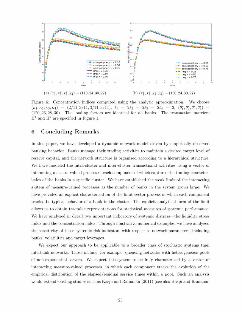
Figure 6 suggests that higher idiosyncratic risk (higher σ) leads to a greater concentration in

monetary reserves. This is intuitively expected because higher volatility increases the variability

of the sample paths of the interbanking network, and thus raises the probability of observing

higher heterogeneity in the distribution of monetary reserves in the network. In line with

intuition, the Herfindahl index is generally higher in the ring network, because a more sparsely

connected network reduces the amount of risk sharing in the network. A larger shock to the

initial monetary reserves of a cluster leads to a higher concentration index both for the ring

and core-periphery network.

22

0 1 2 3 4 5 6 7 8 9 10

time

78

79

80

81

82

83

84

85

conce

ntr

atio

n in

dex

core-periphery = 0.25

core-periphery = 0.50

core-periphery = 0.75

ring = 0.25

ring = 0.50

ring = 0.75

(a) (x∗1, x∗2, x∗3, x∗4) = (110, 24, 30, 27)

0 1 2 3 4 5 6 7 8 9 10

time

78

80

82

84

86

88

90

92

94

conce

ntr

atio

n in

dex

core-periphery = 0.25

core-periphery = 0.50

core-periphery = 0.75

ring = 0.25

ring = 0.50

ring = 0.75

(b) (x∗1, x∗2, x∗3, x∗4) = (100, 24, 30, 27)

Figure 6: Concentration indices computed using the analytic approximation. We choose(κ1, κ2, κ3, κ4) = (2/11, 3/11, 3/11, 3/11), `1 = 2`2 = 2`3 = 2`4 = 2, (θ∗1, θ

∗2, θ∗3, θ∗4) =

(120, 26, 28, 30). The loading factors are identical for all banks. The transaction matricesΠ1 and Π2 are specified in Figure 1.

6 Concluding Remarks

In this paper, we have developed a dynamic network model driven by empirically observed

banking behavior. Banks manage their trading activities to maintain a desired target level of

reserve capital, and the network structure is organized according to a hierarchical structure.

We have modeled the intra-cluster and inter-cluster transactional activities using a vector of

interacting measure-valued processes, each component of which captures the trading character-

istics of the banks in a specific cluster. We have established the weak limit of the interacting

system of measure-valued processes as the number of banks in the system grows large. We

have provided an explicit characterization of the limit vector process in which each component

tracks the typical behavior of a bank in the cluster. The explicit analytical form of the limit

allows us to obtain tractable representations for statistical measures of systemic performance.

We have analyzed in detail two important indicators of systemic distress—the liquidity stress

index and the concentration index. Through illustrative numerical examples, we have analyzed

the sensitivity of these systemic risk indicators with respect to network parameters, including

banks’ volatilities and target leverages.

We expect our approach to be applicable to a broader class of stochastic systems than

interbank networks. Those include, for example, queueing networks with heterogeneous pools

of non-exponential servers. We expect this system to be fully characterized by a vector of

interacting measure-valued processes, in which each component tracks the evolution of the

empirical distribution of the elapsed/residual service times within a pool. Such an analysis

would extend existing studies such as Kaspi and Ramanan (2011) (see also Kaspi and Ramanan

23

(2013) for a second-order refinement via martingale measures), from a one-dimensional to a

high-dimensional setting, with multiple heterogeneous server pools and appropriate routing

rules.

Acknowledgment

We would like to thank the two referees for insightful comments that led to a significant im-

provement of this manuscript. We are also grateful to Ward Whitt and Marty Reiman for

interesting discussions and perceptive comments. We also thank the participants of the 2017

INFORMS Annual Meeting, the 2017 INFORMS Applied Probability Society Meeting, and the

seminar participants of the Financial Mathematics seminars at the University of Connecticut,

and the University of California at Santa Barbara. Agostino Capponi is supported in part by the

NSF/CMMI CAREER-1752326. Xu Sun’s research is supported by NSF grant CMMI-1634133.

David Yao’s research is supported in part by NSF grant CMMI-1462495.

Appendices

We provide the proof of the main theorem in Appendix A. All other proofs are relegated to

Appendix B.

A Proof of Theorem 3.1

The proof consists of three technical steps. The first step is to prove tightness via Lemma A.1

and Proposition A.1; the second step is to identify the weak limit through Propositions A.2 and

A.3; the third step is to prove the uniqueness of the weak limit through Lemma A.2. Taken

together, these steps complete the proof of the main theorem.

Tightness of the Sequence of Measure-Valued Processes. The proof of tightness for the

sequence of measure-valued processes νη(·) is implied by (i) the compact containment condition

(CCC) and (ii) the modulus of continuity condition (MCC). The CCC holds if and only if for

each ε > 0 there exists a compact subset K of S such that, for an arbitrarily fixed T > 0,

infη∈N

P(νη(t) ∈ K for all t ∈ [0, T ]

)> 1− ε. (A.1)

The CCC is often difficult to verify. However, a weaker condition which we will refer to as

pointwise containment condition (PCC) can often be used in conjunction with the MCC to

establish the CCC; see, e.g., Ledger (2016). The PCC holds if for all ε > 0 and t ∈ [0, T ], there

exists a compact set K(ε, t) that depends on both ε and t such that

infη∈N

P(νη(t) ∈ K(ε, t)

)> 1− ε. (A.2)

24

By Proposition 3.1, (S, β) is a complete metric space. Then by Theorem 17 of Ledger

(2016), if the family of S-valued processes νη satisfy both the MCC and the PCC, then the

CCC holds. The forthcoming lemma verifies the PCC.

Lemma A.1 For each ε and t ≥ 0, there exists a compact subset K∗ of S such that

infη∈N

P(νη(t) ∈ K∗(ε, t)

)> 1− ε.

Proof of Lemma A.1 The argument below is adapted from the proof of Lemma 6.1 of

Giesecke et al. (2013), but takes into account that νη is multidimensional. For each M > 0,

define KM ≡ [0, Cp]2 × [0,M ] where Cp is the bound given in Assumption 3. Further, denote

by Ac the complement of a set A. We then have, for each j = 1, . . . , N ,

E[〈νηj , 1KcM 〉t

]= νηj (t)(KcM ) =

1

Kηj

Kηj∑

k=1

P (ξj,k(t) ≥M) ≤ C(1, T, Cp)

M,

where the constant C(1, T, Cp) ≡ C(1, T, Cp)eC(1,T,Cp)T is provided in the proof of Lemma B.1.

Next we define

K∗M ≡µ ≡ (µ1, . . . , µN ) ∈ S : 〈µj , 1Kc

(M+k)2〉 < 1√

M + kfor all j = 1, . . . , N and all k ∈ N

.

Note that, in the above expression, 〈µj , 1A〉 equals the probability µj(A). For each j, the

collection of probability measures

K∗M,j ≡µj : 〈µj , 1Kc

(M+k)2〉 < 1√

M + k

is tight (by the definition of tightness). From Prokhorov’s theorem (see, e.g., Theorem 11.5.4

in Dudley (2002)), it follows that K∗M,j is a compact subset of P(O). Applying Tychonoff’s

Theorem (see, e.g., Theorem 2.2.8 in Dudley (2002)), we conclude that the set K∗M is a compact

subset of S. In addition, we have

P (νη(t) /∈ K∗M ) ≤N∑j=1

∞∑k=1

P(〈νηj , 1Kc(M+k)2

〉t >1√

M + k

)

≤N∑j=1

∞∑k=1

E[〈νηj , 1Kc(M+k)2

〉t]

1/√M + k

≤∞∑k=1

NC(1, T, Cp)

(M + k)2/√M + k

→ 0 as M →∞.

The convergence to zero is independent of the index η. Hence for any ε > 0, by choosing M

large enough, one gets

infη∈N

P(νη(t) ∈ K∗M

)> 1− ε,

as desired.

The PCC will be strengthened to CCC if MCC holds. The following proposition uses

Proposition 3.2 to verify the MCC.

25

Proposition A.1 Let g(x, y) = ‖x − y‖2 ∧ 1 for any x, y ∈ RN and define Et[·] ≡ E[·|Ft] for

t ≥ 0. Then for each γ ≥ 0, there exists a positive random variable aη(γ) that depends on γ

with limγ→0 supη E[aη(γ)] = 0 such that for all 0 ≤ t ≤ T , 0 ≤ u ≤ γ and 0 ≤ v ≤ γ ∧ t,

Et[g2 (〈νη, f〉t+u, 〈νη, f〉t) g2 (〈νη, f〉t, 〈νη, f〉t−v)

]≤ Et [aη(γ)] ,

where f ∈ C2b (O) and 〈νη, f〉t ≡

(〈νη1 , f〉t, . . . , 〈ν

ηN , f〉t

)>.

Proof of Proposition A.1 For notational brevity, in what follows we write f(x) ≡ f(p, x)

whenever it is clear from the context. In view of the equation (B.10), we have

〈νηj , f〉t = 〈νηj , f〉0 +Aj(t) +Bj(t) + Ej(t) + Fj(t), (A.3)

where we have defined

Aj(t) ≡ `j∫ t

0

1

Kηj

Kηj∑

k=1

∂f(ξj,k(s))

∂x(θj,k − ξj,k(s)) ds,

Bj(t) ≡ −∑h≤N

`h,j

∫ t

0

1

Kηj

Kηj∑

k=1

∂f(ξj,k(s))

∂x

(θh − ξh(s)

)ds,

Ej(t) ≡∫ t

0

1

2Kηj

Kηj∑

k=1

σ2j,kξj,k(s)

∂2f(ξj,k(s))

∂x2ds,

Fj(t) ≡∫ t

0

1

Kηj

Kηj∑

k=1

σj,k∂f(ξj,k(s))

∂x(ξj,k(s))

1/2dWj,k(s).

(A.4)

Using the definition of g and (A.4), it follows that

g2 (〈νη, f〉t+u, 〈νη, f〉t) ≤N∑j=1

∣∣∣〈νηj , f〉t+u − 〈νηj , f〉t∣∣∣2≤4

N∑j=1

(|Aj(t+ u)−Aj(t)|2 + |Bj(t+ u)−Bj(t)|2 + |Ej(t+ u)− Ej(t)|2 + |Fj(t+ u)− Fj(t)|2

).

(A.5)

Below, we analyze in turn the terms Aj , Bj , Ej and Fj . First, for 0 ≤ u ≤ γ, we have

|Aj(t+ u)−Aj(t)|2 ≤ C2p

∥∥∥∥∂f∂x∥∥∥∥2

u

∫ t+u

t

(1

Kηj

Kηj∑

k=1

(θj,k − ξj,k(s)))2

ds

≤ C2p

∥∥∥∥∂f∂x∥∥∥∥2

γ

∫ T

0

1

Kηj

Kηj∑

k=1

(θj,k − ξj,k(s)

)2ds ≡ aηj,1(γ),

26

where both the first and the second inequality follow by applying the Cauchy-Schwartz inequal-

ity. Similarly, we have

|Bj(t+ u)−Bj(t)|2 ≤ C2p

∥∥∥∥∂f∂x∥∥∥∥2

γN∑h=1

1

Kηh

∫ T

0

Kηh∑

k′=1

(θh,k − ξh,k(s)

)2ds ≡ aηj,2(γ) and

|Ej(t+ u)− Ej(t)|2 ≤C4p

2

∥∥∥∥∂2f

∂x2

∥∥∥∥2

γ

∫ T

0

1

Kηj

Kηj∑

k=1

|ξj,k(s)|2 ds ≡ aηj,3(γ) for 0 ≤ u ≤ γ.

Finally,

Et[|Fj(t+ u)− Fj(t)|2

]≤ CEt

∫ t+u

t

1

Kηj

Kηj∑

k=1

σj,k∂f(ξj,k(s))

∂x(ξj,k(s))

1/2

2

ds

≤ CEt

C2p

∥∥∥∥∂f∂x∥∥∥∥2 ∫ t+u

t

1

Kηj

Kηj∑

k=1

ξj,k(s)ds

≤ Et

CC2p

2

∥∥∥∥∂f∂x∥∥∥∥2

γ1/4

1 +

∫ T

0

1

Kηj

Kηj∑

k=1

|ξj,k(s)|2 ds

≡ Et[aηj,4(γ)

],

where the first inequality follows by applying the Burkholder-Davis-Gundy inequality with C

being a universal constant and the third inequality uses the technical estimate in (A.6)∫ t

sξj,k(u)du ≤ 1

2(t− s)1/4

(1 +

∫ T

0|ξj,k(u)|2 du

)for 0 ≤ s ≤ t ≤ T, (A.6)

which follows directly from inequality (6.1) in Giesecke et al. (2013), which is in turn an applica-

tion of the Cauchy-Schwartz inequality combined with the geometric/harmonic mean inequality.

Let

aη(γ) ≡N∑j=1

(aηj,1(γ) + aηj,2(γ) + aηj,3(γ) + aηj,4(γ)

).

By Lemma B.1 in Appendix B, we conclude limγ→0 supη E[aη(γ)] = 0. The proof is then

complete by noting that g2 (〈νη, f〉t, 〈νη, f〉t−v) ≤ 1, for v ∈ [0, γ ∧ t].

Identification of the Limit. We formulate and solve the martingale problem that pins down

the limiting measure-valued process. We start by introducing the following operators on the

space C2(O):

T dr0 f = ∂f/∂x, T dr1 f = x(∂f/∂x), T dr2 f = θ(∂f/∂x), T vf = (σ2x/2)(∂2f/∂x2

). (A.7)

Recall that Φ is an element of the function class D defined in (3.8). We identify the generator

of the limiting process as the operator A acting on Φ(·) defined by

AΦ(µ) ≡m∑n=1

N∑j=1

∂φ

∂xj,n

[`j〈µj , T dr2 fj,n〉 − `j〈µj , T dr1 fj,n〉+ 〈µj , T vfj,n〉

−∑h≤N

`h,j〈µj , T dr0 fj,n〉〈µh,Θ− ψ1〉]

for µ ≡ (µ1, . . . , µN ) ∈ S.(A.8)

27

Proposition A.2 The operator A is the generator of our limit martingale problem in the sense

of

limη→∞

E

[(Φ(νη(tr+1))− Φ(νη(tr))−

∫ tr+1

tr

AΦ(νη(u))du

) r∏i=1

Ψi(νη(tj))

]= 0,

where 0 ≤ t1 < . . . < tr+1 < +∞ with r ∈ N, and Ψi ∈ B(S) (the set of all bounded measurable

functions on S), i = 1, . . . , r.

Proof of Proposition A.2 The conclusion follows directly from Lemma B.2 and the fact

that

limη→∞

E[∫ u

t|Eη(s)| ds

]= 0 for 0 ≤ t < u < +∞,

where E is given in (B.9).

Next, we turn to the measure-valued functions ν ≡ (ν1, . . . , νN ) given by (3.16). Our next

result shows that ν solves the martingale problem for A.

Proposition A.3 For the measure-valued functions ν ≡ (ν1, . . . , νN ) given in (3.16) and the

operator A specified by (A.8), it holds that

Φ(ν(t)) = Φ(ν(s)) +

∫ t

sAΦ(ν(u))du for 0 ≤ s < t < +∞. (A.9)

Proof of Proposition A.3 First note that for f ∈ C2(O) we have

〈νj , f〉t =

∫OE [f (pj , Xj(zj ; t))]φj(dzj) for t ≥ 0. (A.10)

where Xj(zj ; t) is defined by (3.9). In what follows, we simply write Xj(t) ≡ Xj(zj ; t) and

f(Xj(t)) ≡ f(pj , Xj(t)). An application of the Ito’s formula yields

f(Xj(t)) = f(xj) + `j

∫ t

0

∂f

∂x(Xj(s)) (θj −Xj(s)) ds−

N∑h=1

`h,j

∫ t

0

∂f

∂x(Xj(s))

(Vh −Qh(s)

)ds

+ σj

∫ t

0

∂f

∂x(Xj(s))

√Xj(s)dWj(s) +

σ2j

2

∫ t

0

∂2f

∂x2(Xj(s))Xj(s)ds.

(A.11)

Taking expectation on both sides and then first-order derivative with respect to t yields

∂

∂tE [f(Xj(t))] = `jE

[T dr2 f(Xj(t))

]− `jE

[T dr1 f(Xj(t))

]+ E [T vf(Xj(t))]

−N∑h=1

`h,jE[T dr0 f(Xj(t))

] (Vh −Qh(t)

)= `jE

[T dr2 f(Xj(t))

]− `jE

[T dr1 f(Xj(t))

]+ E [T vf(Xj(t))]

−N∑h=1

`h,jE[T dr0 f(Xj(t))

] (〈νh,Θ〉t − 〈νh, ψ1〉t

),

28

where the first equality uses the operators given by (A.7) and the second equality follows

from (3.10) and Lemma 3.1. Taking expectation of both sides with respect to the probability

distribution φj , we obtain

∂

∂t

∫OE [f(Xj(t))]φj(dzj) =

∫O

(`jE

[T dr2 f(Xj(t))

]− `jE

[T dr1 f(Xj(t))

]+ E [T vf(Xj(t))]

)φj(dzj)

−N∑

h=1

`h,j

∫OE[T dr0 f(Xj(t))

] (Vh −Qh(t)

)φj(dzj)

=

∫O

(`jE

[T dr2 f(Xj(t))

]− `jE

[T dr1 f(Xj(t))

]+ E [T vf(Xj(t))]

)φj(dzj)

−N∑

h=1

`h,j

∫OE[T dr0 f(Xj(t))

] (〈νh,Θ〉t − 〈νh, ψ1〉t

)φj(dzj).

By Eq. (A.10) and the above equality, we deduce

d〈νj , f〉tdt

= `j〈νj , T dr2 f〉t − `j〈νj , T dr1 f〉t + 〈νj , T vf〉t +N∑h=1

`h,j〈νj , T dr0 f〉t[〈νh,Θ〉t − 〈νh, ψ1〉t

].

(A.12)

Recall the function Φ(ν) defined by (3.8) and the operator A acting on Φ(ν). Using the chain

rule and (A.12), we obtain

dΦ(ν(t))

dt=

m∑n=1

N∑j=1

∂φ

∂xj,n

[`j〈νj , T dr2 fj,n〉t − `j〈νj , T dr1 fj,n〉t + 〈νj , T vfj,n〉t

−N∑h=1

`h,j〈νj , T dr0 fj,n〉t(〈νh,Θ〉t − 〈νh, ψ1〉t

)]≡ AΦ(ν(t)),

which can be rearranged to obtain (A.9).

Lemma A.2 The uniqueness of the martingale problem of the generator A given by (A.8)

holds.

Proof. Our proof follows a duality argument; see e.g., §4.4 in Ethier and Kurtz (2009), p. 182-

195. In particular, duality means that the existence of a solution to the dual problem ensures

uniqueness of a solution to the original problem.

Let C∗ ≡⋃m∈N C∞(ON×m). We start by defining a flow on C∗, as in the proof of Lemma

7.1 in Giesecke et al. (2013). Suppose G ∈ C∗. Then there must exist some m ∈ N such that

G ∈ C∞(ON×m). To begin, let z1:m ≡ (z1, . . . , zm) ∈ ON×m, where for each n ∈ 1, . . . ,m,zn ≡ (z1,n, . . . , zN,n)> with zj,n ≡ (θj,n, σj,n, xj,n) ∈ O, j = 1, . . . , N . Define the spatial diffusion

semigroup:

St : G(z1:m)→ (StG)(z1:m) ≡ (Nm)−1E [G (Y(t))] for Y(t) ≡ (Y1(t), . . . ,Ym(t)) ,

where for each n ∈ 1, . . . ,m, Yn(t) ≡ (Y1,n(t), . . . ,YN,n(t))> with Yj,n(t) ≡ (θj,n, σj,n,Xj,n(t)),

j = 1, . . . , N ; Xj,n is a diffusion process defined by

Xj,n(t) = xj,n + `j

∫ t

0(θj,n −Xj,n(s)) ds+ σj,n

∫ t

0Xj,n(s)dWj,n(s).

29

Wj,n, j = 1, . . . , N, n = 1, . . . ,m, are Brownian motions independent of each other, and of those

in (3.9). Note that each Yj,n (as well as Xj,n) depends on zj,n ≡ (θj,n, σj,n, xj,n). Hence for

t ≥ 0, StG is indeed a function of z1:m. Let us also define the operator Jj,n acting on G ∈ C∗

as a function of its (j, n)-th argument:

Jj,n : G(z1:m)→ (Jj,nG)(z1:m+1) ≡

(N∑h=1

`h,j(xh,m+1 − θh,m+1)

)∂G(z1:m)

∂xj,n. (A.13)

Let us introduce a C∗-valued Markov jump process χ defined through the following procedure:

(i) χ jumps from C∞(ON×m) to C∞(ON×(m+1)) at a rate 1/(Nm); at the time of the jump

let χ(t) be Jj,nχ(t−), where the operator Jj,n is specified by (A.13).

(ii) between jumps, χ(·) evolves deterministically on C∞(ON×m) according to the transfor-

mation semigroup S with infinitesimal generator given by

G ≡ (Nm)−1m∑n=1

N∑j=1

(`jT dr2,(j,n) − `jT

dr1,(j,n) + T v(j,n)

). (A.14)

In particular, using Λj,n; j = 1, . . . , N, n = 1, . . . ,m to denote (Nm) independent Poisson

processes, each with rate 1/(Nm), χ can be expressed as the strong solution to the stochastic

differential equation

dχ(t) = d(χc(t)) +m∑n=1

N∑j=1

[Jj,nχ(t−)− χ(t−)] dΛj,n(t) for t ≥ 0, (A.15)

where we have used the subscript c to denote the continuous part. To proceed, define

Γ(µ,G) ≡∫ON×m

G(z1:m)

m∏n=1

N∏j=1

µj(dzj,n)

for G ∈ C∞(ON×m) and µ ≡ (µ1, . . . , µN ) ∈ S. It is easily checked that

Γ(µ,G) = (Nm)−1m∑n=1

N∑j=1

〈µj , Gj,n(zj,n)〉 (A.16)

where

G(j,n)(zj,n) ≡∫G(z1:m)

∏(i,l)6=(j,n)

µi(dzi,l)

is obtained by integrating out all except the (j, n)-th coordinate of z1:m. Now consider an

S-valued process ν solving the martingale problem for A. Using (A.16) and (A.8) (with φ and

fj,n there being φ([aj,n]N×m) = (Nm)−1∑m

n=1

∑Nj=1 aj,n and G(j,n) respectively), we get

Γ(ν(t), G) =

∫ t

0AΓ(ν(s), G)ds+N1(t), (A.17)

30

where N1 is a martingale and the operator A is specified as follows:

AΓ(µ,G) ≡ (Nm)−1m∑n=1

N∑j=1

∫ON×m

(`jT dr2,(j,n) − `jT

dr1,(j,n) + T v(j,n)

)G(z1:m)

m∏n=1

N∏j=1

µj(dzj,n)

− (Nm)−1m∑n=1

N∑j=1

∫ON×m

∑h≤N

`h,j[〈µh,Θ〉 − 〈µh, ψ1〉

]T dr0,(j,n)G(z1:m)

m∏n=1

N∏j=1

µj(dzj,n),

(A.18)

where for an operator T , the notation T(j,n) means that T operates on the (j, n)-th argument

of the function G. By (A.13) and (A.14), we can rewrite (A.18) as

AΓ(µ,G) = Γ(µ,GG) +m∑n=1

N∑j=1

(Nm)−1 [Γ(µ,Jj,nG)− Γ(µ,G)] + Γ(µ,G). (A.19)

On the other hand, from our construction of the Markov jump process χ, i.e., (A.15), it follows

Γ(µ, χ(t)) =

∫ t

0A#Γ(µ, χ(s))ds+N2(t), (A.20)

where N2 is a martingale and

A#Γ(µ,G) ≡ Γ(µ,GG) +

m∑n=1

N∑j=1

(Nm)−1 [Γ(µ,Jj,nG)− Γ(µ,G)] . (A.21)

Combining (A.19) and (A.21) yields

AΓ(µ,G) = A#Γ(µ,G) + Γ(µ,G), (A.22)

which completes the proof.

By the standard analysis of weak convergence (see §3.7, §3.8, §3.9 in Ethier and Kurtz

(2009), p. 127-146), existence of a weak limit for the sequence of measure-valued processes νη(·)is guaranteed by Lemma A.1 and Proposition A.1; convergence to a solution of the martingale

problem follows from Propositions A.2 and A.3; uniqueness of the martingale problem is ensured

by Lemma A.2. This concludes the proof of Theorem 3.1.

B Proofs of other technical results

Proof of Proposition 3.1 Non-negativity and symmetry are immediate from the definition.

To show sub-additivity, pick arbitrarily µ, µ′, µ′′ from S. By the triangular inequality,

N∑j=1

∣∣∣∣∫ f d(µj − µ′′j )∣∣∣∣ ≤ N∑

j=1

∣∣∣∣∫ f d(µj − µ′j)∣∣∣∣+

N∑j=1

∣∣∣∣∫ f d(µ′j − µ′′j )∣∣∣∣ .

To show indiscernibility, suppose β(µ, µ′) = 0. From the definition (3.7), it follows that for each

j

sup

∣∣∣∣∫ f d(µj − µ′j)∣∣∣∣ : ‖f‖BL ≤ 1

= 0.

31

The above expression simply means that β(µj , µ′j) = 0, which in turn implies ρ(µj , µ

′j) = 0,

where we recall that ρ denotes the Prokhorov metric. Thus µj = µ′j in a sense that µj(A) =

µ′j(A) for all Borel set in O. Note that the equality holds for all j ≤ N . We therefore conclude

that µ = µ′.

Proof of Proposition 3.3 Denote by D0 the class of functions of the form

Φ(µ) = φ (〈µ, f1〉, . . . , 〈µ, fm〉) ,

where 〈µ, fn〉 ≡ (〈µ1, fn〉, . . . , 〈µN , fn〉)>, n = 1, . . . ,m, for some m ∈ Z+, fn ∈ C∞(O) and

φ ∈ C∞(RN×m). Clearly, D0 is a subset of the function class D given by (3.8). Thus, in order to

prove the proposition, it suffices to show that the function class D0 has the desired properties.

To this purpose, pick arbitrarily µ, µ′ from the product space S and suppose µ 6= µ′. Then we

must have β(µ, µ′) = ε for some ε > 0. Setting ε ≡ ε/N , take a compact set K ⊂ O such that

µj(K) > 1− ε/8 and µ′j(K) > 1− ε/8 for all j = 1, . . . , N . By the Arzela-Ascoli theorem, the

set of functions B ≡ f : ‖f‖BL ≤ 1 restricted to K forms a compact set of functions for the

norm ‖ · ‖∞. Thus there exist f1, f2, . . . , fm ∈ B for some m ∈ N such that for any f ∈ B, there

exists fi satisfying supx∈K |f(x)− fi(x)| < ε/8. By the triangular inequality,

|〈µj , f〉 − 〈µ′j , f〉| ≤ |〈µj , f〉 − 〈µj , fi〉|+ |〈µ′j , f〉 − 〈µ′j , fi〉|+ |〈µj , fi〉 − 〈µ′j , fi〉|

for j = 1, . . . , N . The first term on the right hand side

|〈µj , f〉 − 〈µj , fi〉| ≤ |〈µj , (f − fi)1Kc〉|+ |〈µj , (f − fi)1K〉| < ε/4 + ε/8 = 3ε/8,

where the second inequality uses the fact that ‖f − fi‖ ≤ 2 and that µj(Kc) ≤ ε/8. Similarly

for the second term we have |〈µ′j , f〉 − 〈µ′j , fi〉| < 3ε/8. Combining the above yields

|〈µj , f〉 − 〈µ′j , f〉| < 3ε/4 + maxi≤m|〈µj , fi〉 − 〈µ′j , fi〉|. (B.1)

Adding up (B.1) over j = 1, . . . , N , we get

N∑j=1

|〈µj , f〉 − 〈µ′j , f〉| < 3ε/4 +

N∑j=1

maxi≤m|〈µj , fi〉 − 〈µ′j , fi〉|.

Because f is arbitrarily chosen from B and β(µ, µ′) = ε, the right-hand side of (B.1) must

be greater or equal to ε. Hence, there exist i ∈ 1, . . . ,m and j ∈ 1, . . . , N such that

|〈µj , fi〉 − 〈µ′j , fi〉| ≥ ε/(4N) ≡ ε/4. On the other hand, any globally Lipschitz continuous

function can be approximated by a sequence of infinitely differentiable functions. We can

therefore find f ∈ C∞(O) satisfying |〈µj , f〉 − 〈µ′j , f〉| ≥ ε/8. The first part of the conclusion

follows immediately from the the fact that C∞(RN×m) separates points in RN×m. Since D0

forms a subalgebra, an application of Stone-Weierstrass Theorem gives the second part of the

conclusion.

32

Proof of Lemma 3.1 From the definition (3.12), it follows immediately that

〈νj , ψ1〉t ≡∫OE [Xj(zj ; t)]φj(dzj) for t ≥ 0, (B.2)

where we recall that the underlying state process Xj(zj ; t) follows the SDE given in (3.9).

It follows from the same equation (3.9) that the expectation E[Xj(zj ; t)] satisfies the integral

equation below:

E [Xj(zj ; t)] = xj+

∫ t

0`j (θj − E [Xj(zj ; s)]) ds−

∫ t

0

N∑h=1

`h,j (Vh −Qh(s)) ds for t ≥ 0. (B.3)

The integral equation (B.3) admits an explicit solution:

E [Xj(zj ; t)] = e−`jt

[xj +

∫ t

0

(`jθj −

N∑h=1

`h,j (Vh −Qh(s))

)e`jsds

]. (B.4)

Combining (B.2) and (B.4) completes the proof of the lemma.

Proof of Proposition 5.1 Our objective is to find functions α(·, u) and β(·, u) with α(0, u) =

0 and β(0, u) = u such that

M(s) ≡ g(s,X(s)) ≡ exp [α(t− s, u) + β(t− s, u)X(s)] , for 0 ≤ s ≤ t,

is martingale. If this is the case, then

E[euX(t)

]= E [M(t)] =M(0) = exp [α(t, u) + β(t, u)X(0)] .

An application of the Ito’s formula to g(s,X(s)) yields

dg(s,X(s))

g(s,X(s))= −

[α′(t− s, u) +X(s)β′(t− s, u)

]ds+ β(t− s, u)`(θ −X(s))ds

+ q(s)β(t− s, u)ds+ β(t− s, u)X(s)dW (s) +1

2σ2X(s)β(t− s, u)2ds,

where we have used α′ and β′ to denote, respectively, the first-order derivatives of α and β with

respect to the first argument. Then g(s,X(s)) is a martingale if the drift term vanishes, i.e., if

α′(t− s, u) +X(s)β′(t− s, u) = β(t− s, u)`(θ −X(s)) + q(s)β(t− s, u) +1

2σ2X(s)β(t− s, u)2

for all possible states of X(s). By setting the drift term to zero, we obtain immediately the

following system of non-linear differential equations

α′(s, u) = `θβ(s, u) + q(t− s)β(s, u) and

β′(s, u) = −`θβ(s, u) +σ2

2β(s, u)2

with initial conditions α(0, u) = 0 and β(0, u) = u. The set of differential equations admits the

solution specified in (5.2).

Lemma B.1 If Assumption 3 is satisfied, then for any finite T > 0 and n ∈ N, we have

supη

sup0≤t≤T

N∑j=1

1

Kηj

Kηj∑

k=1

E [|ξj,k(t)|n] < +∞. (B.5)

33

Proof of Lemma B.1 Recall from Eq. (2.2) that

ξj,k(t) = ξj,k(0)+

∫ t

0`j [θj,k − ξj,k(s)] ds−

∫ t

0

N∑h=1

`h,j[θh − ξh(s)

]ds+σj,k

∫ t

0

√ξj,k(s)dWj,k(s).

An application of the Ito’s formula to the smooth function f(ξj,k(t)), where f(x) = xn, gives

(ξj,k(t))n = (ξj,k(0))n + n

∫ t

0`j (ξj,k(s))

n−1 [θj,k − ξj,k(s)] ds+n(n− 1)

2

∫ t

0σ2j,k (ξj,k(t))

n−1 ds

− n∫ t

0

N∑h=1

`h,j (ξj,k(t))n−1 [θh − ξh(s)

]ds+ n

∫ t

0σj,k (ξj,k(t))

n−1/2 dWj,k(s)

≤ (ξj,k(0))n + n

∫ t

0`jθj,k (ξj,k(s))

n−1 ds+n(n− 1)

2

∫ t

0σ2j,k (ξj,k(t))

n−1 ds

+ n

∫ t

0

N∑h=1

`h,j (ξj,k(t))n−1 ξh(s)ds+ n

∫ t

0σj,k (ξj,k(t))

n−1/2 dWj,k(s).

(B.6)

where the inequality follows from the positivity of those ξj,k. An application of Young’s in-

equality yields

(ξj,k(s))n−1 ≤ (n− 1) (ξj,k(s))

n /n+ 1/n

and

(ξj,k(s))n−1 ξh,k′(s) ≤ (n− 1) (ξj,k(s))

n /n+(ξh,k′(s)

)n/n.

It then follows that

(ξj,k(s))n−1 ξh(s) ≤ (n− 1) (ξj,k(s))

n /n+1

Kηh

Kηh∑

k′=1

(ξh,k′(s)

)n/n.

Combining the preceding inequalities with (B.6), we have

E [(ξj,k(t))n] ≤ E [(ξj,k(0))n] +Cn

∫ t

0E [(ξj,k(s))

n] ds+Cn

∫ t

0

N∑j=1

1

Kηj

Kηj∑

k=1

E [(ξj,k(s))n] ds+Cnt,

(B.7)

where Cn is a constant that only depends on Cp (given in Assumption 3) and n. We can

therefore conclude that

N∑j=1

1

Kηj

Kηj∑

k=1

E [(ξj,k(t))n] ≤

N∑j=1

1

Kηj

Kηj∑

k=1

E [(ξj,k(0))n] + Cn

∫ t

0

N∑j=1

1

Kηj

Kηj∑

k=1

E [(ξj,k(s))n] ds

+NCn

∫ t

0

N∑j=1

1

Kηj

Kηj∑

k=1

E [(ξj,k(s))n] ds+NCnt.

An application of the Gronwall’s inequality then gives

N∑j=1

1

Kηj

Kηj∑

k=1

E [(ξj,k(t))n] ≤ C(n, T, Cp)e

C(n,T,Cp)T for all 0 ≤ t ≤ T .

34

The result follows from the fact that the bound on the right hand side of the above inequality

is independent of t and η.

Lemma B.2 Let 0 ≤ t < u < +∞. It holds that,

Φ(νη(u)) = Φ(νη(t)) +

∫ u

tDη(s)ds+

∫ u

tEη(s)ds+ M(u)− M(t), (B.8)

where (Mt; t ≥ 0) is a (P,F)-(local) martingale, and

Dη(t) ≡m∑n=1

N∑j=1

∂φ

∂xj,n

[`j〈νηj , T

dr2 fj,n〉t − `j〈νηj , T

dr1 fj,n〉t + 〈νηj , T

vfj,n〉t,

−∑h≤N

`h,j〈νηj , Tdr

0 fj,n〉t(〈νηh,Θ〉t − 〈ν

ηh, ψ1〉t

) ]

Eη(t) ≡m∑

l,n=1

N∑j=1

∂2φ

∂xj,l∂xj,n· 1

2(Kηj )2

Kηj∑

k=1

[σ2j,k

∂fj,l(ξj,k(t))

∂x

∂fj,n(ξj,k(t))

∂xξj,k(t)

]. (B.9)

Proof of Lemma B.2 First applying Ito’s formula to f(ξj,k(t)) and then taking the average

over k ∈ 1, . . . ,Kj yields

〈νηj , f〉t = 〈νηj , f〉0 + `j

∫ t

0〈νηj , T

dr2 f〉sds− `j

∫ t

0〈νηj , T

dr1 f〉sds+

1

Kηj

Kηj∑

k=1

Mj,k(t)

−N∑h=1

`h,j

∫ t

0〈νηj , T

dr0 f〉s

[〈νηh,Θ〉s − 〈ν

ηh, ψ1〉s

]ds+

∫ t

0〈νηj , T

vf〉sds,

(B.10)

where the operators T dri , i = 0, 1, 2 and T v are given by (A.7), and the (P,F)-(local) martingale

is given by

Mj,k(t) ≡∫ t

0σj,k

∂f(ξj,k(s))

∂x(ξj,k(s))

1/2dWj,k(s). (B.11)

Replacing µ with νη(t) in (3.8) and applying Ito’s formula yields (B.8).

References

Acemoglu D, Ozdaglar A, Tahbaz-Salehi A (????) Systemic risk and stability in financial networks.American Economic Review 105(2):564–608.

Acharya V, Anginer D, Warburton A (2014) The end of market discipline? Investor expectations ofimplicit government guarantees. Working Paper, New York University .

Adrian T, Shin H (2010) Liquidity and leverage. Journal of Financial Intermediation 19(3):418–437.

Afonso G, Kovner A, Schoar A (2013) Trading partners in the interbank lending market. FRB of NewYork Staff Report (620).

Berger AN, DeYoung R, Flannery MJ, Lee D, Oztekin O (2008) How do large banking organizationsmanage their capital ratios? Journal of Financial Services Research 34(2-3):123–149.

Bo L, Capponi A (2014) Bilateral credit valuation adjustment for large credit derivatives portfolios.Finance and Stochastics 18(2):431–482.

Bo L, Capponi A (2015) Systemic risk in interbanking networks. SIAM Journal on Financial Mathe-matics 6(1):386–424.

35

Capponi A (2016) Systemic risk, policies, and data needs. INFORMS Tutorials in Operations Research:Optimization Challenges in Complex, Networked and Risky Systems, 185–206 (INFORMS).

Capponi A, Chen P, Yao D (2016) Liability concentration and systemic losses in financial networks.Operations Research 64(5):1121–1134.

Cetorelli N, McAndrews J, Traina J (2014) Evolution in bank complexity. Economic Policy Review20(2):85–106.

Cocco JF, Gomes FJ, Martins NC (2009) Lending relationships in the interbank market. Journal ofFinancial Intermediation 18(1):24–48.

Craig B, Von Peter G (2014) Interbank tiering and money center banks. Journal of Financial Interme-diation 23(3):322–347.

Dawson D, Kurtz T (1982) Applications of duality to measure-valued diffusion processes. Advances inFiltering and Optimal Stochastic Control 91–105.

Dudley RM (2002) Real analysis and probability, volume 74 (Cambridge University Press).

Duffie D, Kan R (1996) A yield-factor model of interest rates. Mathematical finance 6(4):379–406.

Eisenberg L, Noe TH (2001) Systemic risk in financial systems. Management Science 47(2):236–249.

Ethier SN, Kurtz TG (2009) Markov processes: characterization and convergence, volume 282 (JohnWiley & Sons).

Fouque JP, Ichiba T (2013) Stability in a model of interbank lending. SIAM Journal on FinancialMathematics 4(1):784–803.

Fricke D, Lux T (2015) Core-periphery structure in the overnight money market: Evidence from thee-mid trading platform. Computational Economics 45(3):359–395.

Giesecke K, Sirignano J, Spiliopoulos K, Sower R (2015) Large portfolio asymptotics for loss from default.Mathematical Finance 25(1):77–114.

Giesecke K, Spiliopoulos K, Sowers RB (2013) Default clustering in large portfolios: Typical events. TheAnnals of Applied Probability 23(1):348–385.

Glasserman P, Young P (2015) How likely is contagion in financial networks? Journal of Banking andFinance 50:383–399.

Glasserman P, Young P (2016) Contagion in financial networks. Journal of Economic Literature54(3):779–831.

Gromoll HC, Robert P, Zwart B (2008) Fluid limits for processor-sharing queues with impatience.Mathematics of Operations Research 33(2):375–402.

Gropp R, Heider F (2010) The determinants of bank capital structure. Review of Finance 14(4):587–622.

Ha laj G, Kok C (2013) Assessing interbank contagion using simulated networks. Computational Man-agement Science 10(2-3):157–186.

Jennings OB, Puha AL (2013) Fluid limits for overloaded multiclass fifo single-server queues with generalabandonment. Stochastic Systems 3(1):262–321.

Kaspi H, Ramanan K (2011) Law of large numbers limits for many-server queues. The Annals of AppliedProbability 21(1):33–114.

Kaspi H, Ramanan K (2013) SPDE limits of many-server queues. The Annals of Applied Probability23(1):145–229.

Ledger S (2016) Skorokhod’s M1 topology for distribution-valued processes. Electronic Communicationsin Probability 21(34):984–1053.

Memmel C, Raupach P (2010) How do banks adjust their capital ratios? Journal of Financial Interme-diation 19(4):509–528.

O’Hara M, Shaw W (1990) Deposit insurance and wealth effects: the value of being “too big to fail”.The Journal of Finance 45(5):1587–1600.

Protter PE (2005) Stochastic Differential Equations (Springer).

Rogers C, Veraart L (2013) Failure and rescue in an interbank network. Management Science 59(4):882–898.

Spiliopoulos K, Sirignano JA, Giesecke K (2014) Fluctuation analysis for the loss from default. StochasticProcesses and their Applications 124(7):2322–2362.

36

Stroock DW, Varadhan SR (1972) On the support of diffusion processes with applications to the strongmaximum principle. Proceedings of the Sixth Berkeley Symposium on Mathematical Statistics andProbability (Univ. California, Berkeley, Calif., 1970/1971), volume 3.

Whitt W (2002) Stochastic-process limits: an introduction to stochastic-process limits and their applica-tion to queues (Springer Science & Business Media).

37