An Efficient Extension to Elevation Maps forOutdoor Terrain Mapping and Loop Closing

Patrick Pfaff Rudolph Triebel Wolfram Burgard

Department of Computer Science, University of Freiburg, 79110 Freiburg, Germany

{pfaff,triebel,burgard}@informatik.uni-freiburg.de

Abstract

Elevation maps are a popular data structure for representing the environmentof a mobile robot operating outdoors or on not-flat surfaces.Elevation maps storein each cell of a discrete grid the height of the surface at thecorresponding place inthe environment. However, the use of this 21

2-dimensional representation, is disad-vantageous when utilized for mapping with mobile robots operating on the ground,since vertical or overhanging objects cannot be represented appropriately. Further-more, such objects can lead to registration errors when two elevation maps haveto be matched. In this paper, we propose an approach that allows a mobile robotto deal with vertical and overhanging objects in elevation maps. Our approachclassifies the points in the environment according to whether they correspond tosuch objects or not. We also present a variant of the ICP algorithm that utilizesthe classification of cells during the data association. Additionally, we describehow the constraints computed by the ICP algorithm can be applied to determineglobally consistent alignments. Experiments carried out with a real robot in anoutdoor environment demonstrate that our approach yields highly accurate eleva-tion maps even in the case of loops. We furthermore present experimental resultsdemonstrating that our classification increases the robustness of the scan matchingprocess.

1 Introduction

The problem of learning maps with mobile robots has been intensively studied in thepast. In the literature, different techniques for representing the environment of a mobilerobot prevail. Topological maps aim at representing environments by graph-like struc-tures, where nodes correspond to places, and edges to paths between them. Geometricmodels, in contrast, use either grid-based approximationsor geometric primitives forrepresenting the environment. Whereas topological maps have the advantage to betterscale to large environments, they lack the ability to represent the geometric structureof the environment. The latter, however, is essential in situations, in which robots aredeployed in unstructured outdoor environments where the ability to traverse specificareas of interest needs to be known accurately. However, full three-dimensional mod-

1

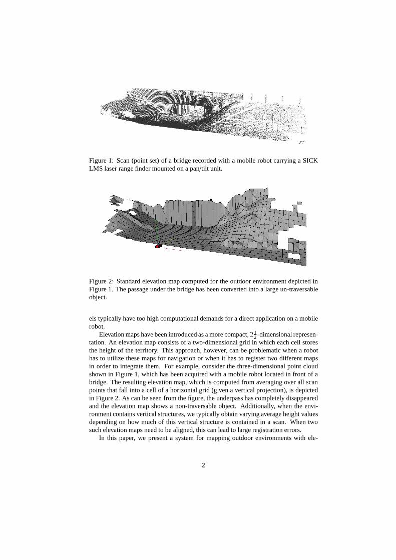
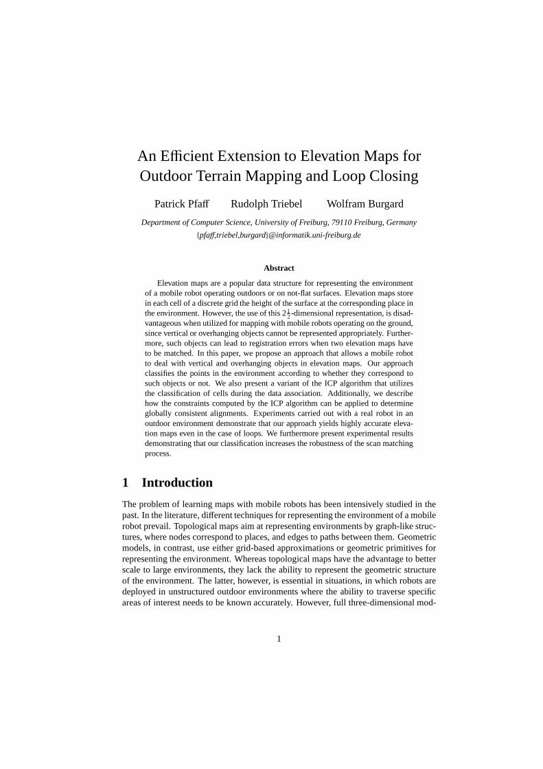
Figure 1: Scan (point set) of a bridge recorded with a mobile robot carrying a SICKLMS laser range finder mounted on a pan/tilt unit.

Figure 2: Standard elevation map computed for the outdoor environment depicted inFigure 1. The passage under the bridge has been converted into a large un-traversableobject.

els typically have too high computational demands for a direct application on a mobilerobot.

Elevation maps have been introduced as a more compact, 212-dimensional represen-

tation. An elevation map consists of a two-dimensional gridin which each cell storesthe height of the territory. This approach, however, can be problematic when a robothas to utilize these maps for navigation or when it has to register two different mapsin order to integrate them. For example, consider the three-dimensional point cloudshown in Figure 1, which has been acquired with a mobile robotlocated in front of abridge. The resulting elevation map, which is computed fromaveraging over all scanpoints that fall into a cell of a horizontal grid (given a vertical projection), is depictedin Figure 2. As can be seen from the figure, the underpass has completely disappearedand the elevation map shows a non-traversable object. Additionally, when the envi-ronment contains vertical structures, we typically obtainvarying average height valuesdepending on how much of this vertical structure is contained in a scan. When twosuch elevation maps need to be aligned, this can lead to largeregistration errors.

In this paper, we present a system for mapping outdoor environments with ele-

2

vation maps. Our approach classifies locations in the environment into four classes,namely locations sensed from above, vertical structures, vertical gaps, and traversablecells. The advantage of this classification is twofold. First, the robot can representobstacles corresponding to vertical structures like wallsof buildings. It also can dealwith overhanging structures like branches of trees or bridges. Second, the classifica-tion can be applied to achieve a more robust data associationin the ICP algorithm [4].In this paper we also describe how to apply a constraint-based robot pose estimationtechnique [33], similar to the one presented by Lu & Milios [17], to calculate globallyconsistent alignments of the local elevation maps. We present experimental results il-lustrating the advantages of our approach regarding the representation aspect as wellas regarding the robust matching in urban outdoor environments also containing loops.

This paper is organized as follows. After discussing related work in the followingsection, we will present our extension to the elevation mapsin Section 3. In Section 4we then describe how to incorporate our classification into the ICP algorithm used formatching elevation maps. Section 5 will introduce our constraint-based pose estimationprocedure for calculating consistent maps. Finally, we present experimental results inSection 6.

2 Related Work

The problem of learning three-dimensional representations has been studied intensivelyin the past. Recently, several techniques for acquiring three-dimensional data with 2drange scanners installed on a mobile robot have been developed. A popular approach isto use multiple scanners that point towards different directions [29, 9, 30]. An alterna-tive is to use pan/tilt devices that sweep the range scanner in an oscillating way [25, 20].More recently, techniques for rotating 2d range scanners have been developed [13, 36].

Many authors have studied the acquisition of three-dimensional maps from vehi-cles that are assumed to operate on a flat surface. For example, Thrun et al. [29]present an approach that employs two 2d range scanners for constructing volumetricmaps. Whereas the first is oriented horizontally and is used for localization, the secondpoints towards the ceiling and is applied for acquiring 3d point clouds. Fruh and Za-khor [7] apply a similar idea to the problem of learning large-scale models of outdoorenvironments. Their approach combines laser, vision, and aerial images. Furthermore,several authors have considered the problem of simultaneous mapping and localization(SLAM) in an outdoor environment [6, 8, 31]. These techniques extract landmarksfrom range data and calculate the map as well as the pose of thevehicles based onthese landmarks. Our approach described in this paper does not rely on the assumptionthat the surface is flat. It uses elevation maps to capture thethree-dimensional structureof the environment and is able to estimate the pose of the robot in all six degrees offreedom.

One of the most popular representations are raw data points or triangle meshes [1,15, 25, 32]. Whereas these models are highly accurate and caneasily be textured, theirdisadvantage lies in the huge memory requirement, which grows linearly in the numberof scans taken. Accordingly, several authors have studied techniques for simplifyingpoint clouds by piecewise linear approximations. For example, Hahnelet al. [9] use

3

a region growing technique to identify planes. Liuet al. [16] as well as Martin andThrun [18] apply the EM algorithm to cluster range scans intoplanes. Recently, Triebelet al. [34] proposed a hierarchical version that takes into account the parallelism ofthe planes during the clustering procedure. An alternativeis to use three-dimensionalgrids [21] or tree-based representations [27], which only grow linearly in the size of theenvironment. Still, the memory requirements for such maps in outdoor environmentsare high.

In order to avoid the complexity of full three-dimensional maps, several researchershave considered elevation maps as an attractive alternative. The key idea underlyingelevation maps is to store the 21

2-dimensional height information of the terrain in atwo-dimensional grid. Bareset al. [3] as well as Hebertet al. [10] use elevation mapsto represent the environment of a legged robot. They extractpoints with high surfacecurvatures and match these features to align maps constructed from consecutive rangescans. Parraet al. [24] represent the ground floor by elevation maps and use stereovision to detect and track objects on the floor. Singh and Kelly [28] extract elevationmaps from laser range data and use these maps for navigating an all-terrain vehicle.Ye and Borenstein [37] propose an algorithm to acquire elevation maps with a movingvehicle carrying a tilted laser range scanner. They proposespecial filtering algorithmsto eliminate measurement errors or noise resulting from thescanner and the motions ofthe vehicle. Lacroixet al. [14] extract elevation maps from stereo images. Hygounencet al. [12] construct elevation maps with an autonomous blimp using 3d stereo vision.They propose an algorithm to track landmarks and to match local elevation maps us-ing these landmarks. Olson [23] describes a probabilistic localization algorithm for aplanetary rover that uses elevation maps for terrain modeling. Wellingtonet al. [35]construct a representation based on Markov Random Fields. They propose an environ-ment classification for agricultural applications. They compute the elevation of the celldepending on the classification of the cell and its neighbors. Compared to these tech-niques, the contribution of this paper lies in two aspects. First, we classify the pointsin the elevation map into horizontal points seen from above,vertical points, and gaps.This classification is important especially when a rover is deployed in an urban envi-ronment. In such environments, typical structures like thewalls of buildings cannotbe represented in standard elevation maps. Second, we describe how this classificationcan be used to improve the matching of different elevation maps.

Recently, several authors have studied the problem of simultaneous localizationand mapping by taking into account the six degrees of freedomof a mobile robot op-erating on a non-flat surface. For example, Davisonet al. [5] presented an approachto vision based SLAM with a single camera moving freely through the environment.This approach uses an extended Kalman Filter to simultaneously update the pose ofthe camera and the 3d feature points extracted from the camera images. More recently,Nuchteret al. [22] developed a mobile robot that builds accurate three-dimensionalmodels. In this approach, loop closing is achieved by uniformly distributing the esti-mated odometry error over the poses in a loop. In contrast, the work described hereemploys elevation maps to obtain a more compact representation of the 3d data. Ourapproach also includes a technique to globally optimize thepose estimates for calcu-lating consistent maps. The loop-closing technique is alsoan extension to our previouswork [26] in which the ICP algorithm was used for incrementalmapping.

4

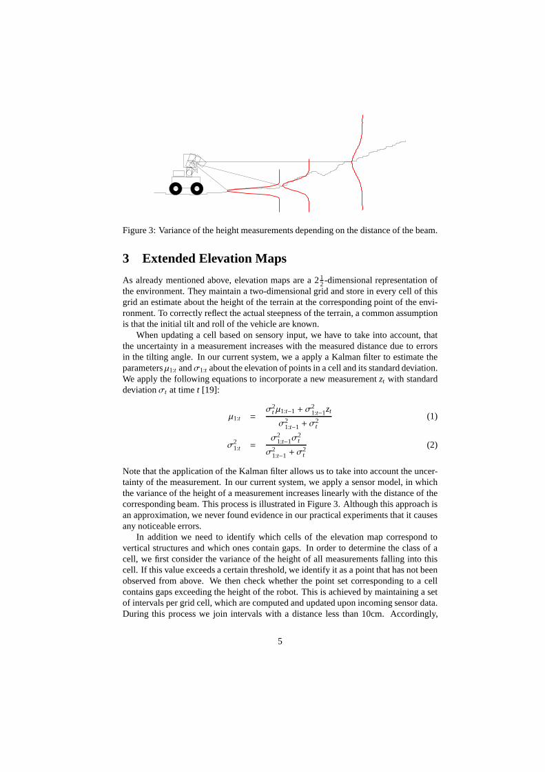
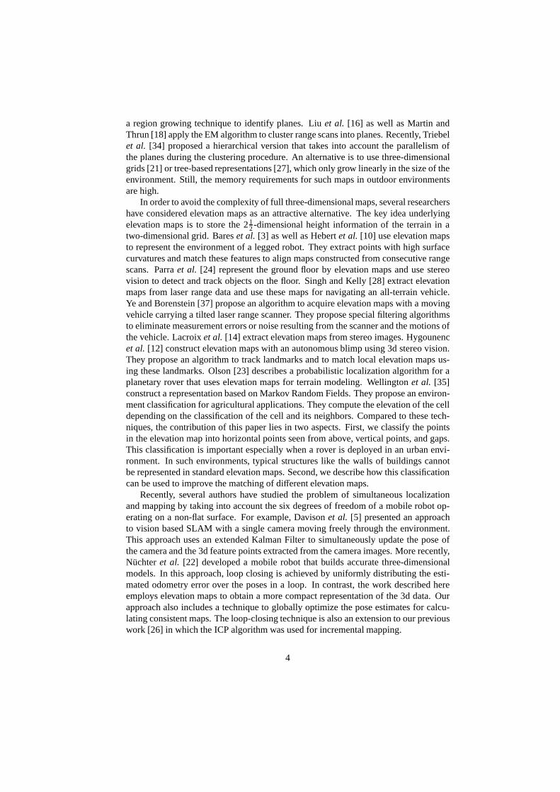
Figure 3: Variance of the height measurements depending on the distance of the beam.

3 Extended Elevation Maps

As already mentioned above, elevation maps are a 212-dimensional representation of

the environment. They maintain a two-dimensional grid and store in every cell of thisgrid an estimate about the height of the terrain at the corresponding point of the envi-ronment. To correctly reflect the actual steepness of the terrain, a common assumptionis that the initial tilt and roll of the vehicle are known.

When updating a cell based on sensory input, we have to take into account, thatthe uncertainty in a measurement increases with the measured distance due to errorsin the tilting angle. In our current system, we a apply a Kalman filter to estimate theparametersµ1:t andσ1:t about the elevation of points in a cell and its standard deviation.We apply the following equations to incorporate a new measurementzt with standarddeviationσt at timet [19]:

µ1:t =σ2

t µ1:t−1 + σ21:t−1zt

σ21:t−1 + σ

2t

(1)

σ21:t =

σ21:t−1σ

2t

σ21:t−1 + σ

2t

(2)

Note that the application of the Kalman filter allows us to take into account the uncer-tainty of the measurement. In our current system, we apply a sensor model, in whichthe variance of the height of a measurement increases linearly with the distance of thecorresponding beam. This process is illustrated in Figure 3. Although this approach isan approximation, we never found evidence in our practical experiments that it causesany noticeable errors.

In addition we need to identify which cells of the elevation map correspond tovertical structures and which ones contain gaps. In order todetermine the class of acell, we first consider the variance of the height of all measurements falling into thiscell. If this value exceeds a certain threshold, we identifyit as a point that has not beenobserved from above. We then check whether the point set corresponding to a cellcontains gaps exceeding the height of the robot. This is achieved by maintaining a setof intervals per grid cell, which are computed and updated upon incoming sensor data.During this process we join intervals with a distance less than 10cm. Accordingly,

5

Figure 4: Labeling of the data points depicted in Figure 1 according to their classifica-tion. The four different classes are indicated by different colors/grey levels.

Figure 5: Extended elevation map for the scene depicted in Figure 1.

it may happen, that the classification of a particular cell needs to be changed fromthe label ’vertical cell’ or ’cell that was sensed from above’ to the label ’gap cell’.Additionally, it can happen in the case of occlusions that a cell changes from the state’gap cell’ to the state ’vertical cell’. When a gap has been identified, we determine theminimum traversable elevation in this point set.

Figure 4 shows the same data points already depicted in Figure 1. The classes of theindividual cells in the elevation map are indicated by the different colors/grey levels.The blue/dark points indicate the data points which are above a gap. The red/mediumgrey values indicate cells that are classified as vertical. The green/light grey values,however, indicate traversable terrain. Note that the non-traversable cells are not shownin this figure.

A major part of the resulting elevation map computed from this data set is shownin Figure 5, in which we only plot the height values for the lowest interval in each cell.As a result, the area under the bridge now appears as a traversable surface. This allowsthe robot to plan a safe path through the underpass.

6

4 Matching Elevation Maps in 6 Dimensions

To calculate the alignments between two local elevation maps generated from indi-vidual scans, we apply the Iterative Closest Point (ICP) algorithm. The goal of thisprocess is to find a rotation matrixR and a translation vectort that minimize an ap-propriate error function. Assuming that the two scans are represented by point setsX = {x1, . . . , xN1} andY = {y1, . . . , yN2}, the algorithm first computes a set ofC indexpairs orcorrespondences(i1, j1), . . . , (iC, jC) such that the pointxic in X corresponds tothe pointy jc in Y, for c = 1, . . . ,C. Then, in a second step, the error function

e(R, t) :=1C

C∑

c=1

(xic − (Ry jc + t))TΣ−1(xic − (Ry jc + t)) (3)

is minimized. Here,Σ denotes the covariance matrix of the Gaussian corresponding toeach pair (xi, yi). In other words, the error functione is defined by the sum of squaredMahalanobis distances between the pointsxic and the transformed pointy jc. In thefollowing, we denote this Mahalanobis distance asd(xic, y jc).

In principle, one could define this function to directly operate on the height valuesand their variance when aligning two different elevation maps. The disadvantage of thisapproach, however, is that in the case of vertical objects, the resulting height stronglydepends on the view point. The same vertical structure may lead to varying heightsin the elevation map when sensed from different points. In practical experiments, weobserved that this introduces serious errors and often prevents the ICP algorithm fromconvergence. To overcome this problem, we separate Equation (3) into four compo-nents each minimizing the error over four different classes of points. These four classescorrespond to cells containing vertical objects, gap cells, traversable cells, and edgecells. In this context, traversable cells are those for which the elevation of the surfacenormal obtained from a plane fitted to the local neighborhoodexceeds a threshold of 83degrees. Edge cells are cells that lie more than 20cm above their neighboring points.

Let us assume thatuic and u′jc are corresponding vertical points,vic and v′jc arevertical gap cells,wic andw′jc are edge points, andx jc andx′jc are traversable cells. Theresulting error function then is

e(R, t) =1C

C1∑

c=1

dv(uic , u′jc)

︸ ︷︷ ︸

vertical objects

+

C2∑

c=1

d(vic, v′jc)

︸ ︷︷ ︸

vertical gaps

+

C3∑

c=1

d(wic,w′jc)

︸ ︷︷ ︸

edge cells

+

C4∑

c=1

d(xic, x′jc)

.

︸ ︷︷ ︸

traversable cells

(4)

In this equation, the distance functiondv calculates the Mahalanobis distance betweenthe lowest points in the particular cells. Note that the sum in Equation (3) has beensplit into four different sums of distances and thatC = C1 +C2 +C3 +C4.

To increase the efficiency of the matching process, we only consider a subset ofthese cells by sub-sampling. In case there are not enough cells in the individual classes,we randomly select an appropriate number of cells (approximately 1,000). This waywe obtain an approach that allows to match elevation maps even in the absence offeatures. In such a situation, our technique becomes equivalent to a standard approach,in which the complete or a random subset of all cells is used for matching.

7

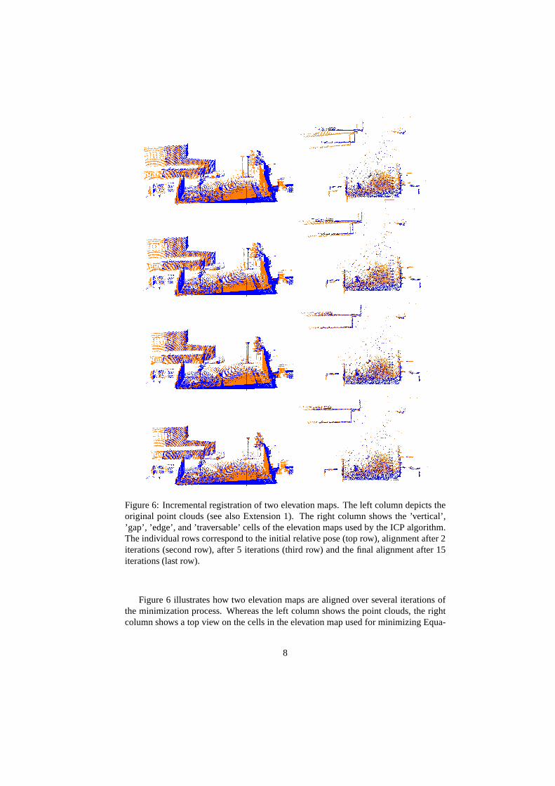
Figure 6: Incremental registration of two elevation maps. The left column depicts theoriginal point clouds (see also Extension 1). The right column shows the ’vertical’,’gap’, ’edge’, and ’traversable’ cells of the elevation maps used by the ICP algorithm.The individual rows correspond to the initial relative pose(top row), alignment after 2iterations (second row), after 5 iterations (third row) andthe final alignment after 15iterations (last row).

Figure 6 illustrates how two elevation maps are aligned overseveral iterations ofthe minimization process. Whereas the left column shows thepoint clouds, the rightcolumn shows a top view on the cells in the elevation map used for minimizing Equa-

8

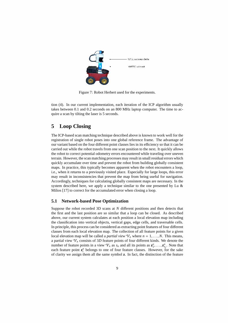
Figure 7: Robot Herbert used for the experiments.

tion (4). In our current implementation, each iteration of the ICP algorithm usuallytakes between 0.1 and 0.2 seconds on an 800 MHz laptop computer. The time to ac-quire a scan by tilting the laser is 5 seconds.

5 Loop Closing

The ICP-based scan matching technique described above is known to work well for theregistration of single robot poses into one global reference frame. The advantage ofour variant based on the four different point classes lies in its efficiency so that it can becarried out while the robot travels from one scan position tothe next. It quickly allowsthe robot to correct potential odometry errors encounteredwhile traveling over uneventerrain. However, the scan matching processes may result insmall residual errors whichquickly accumulate over time and prevent the robot from building globally consistentmaps. In practice, this typically becomes apparent when therobot encounters a loop,i.e., when it returns to a previously visited place. Especially for large loops, this errormay result in inconsistencies that prevent the map from being useful for navigation.Accordingly, techniques for calculating globally consistent maps are necessary. In thesystem described here, we apply a technique similar to the one presented by Lu &Milios [17] to correct for the accumulated error when closing a loop.

5.1 Network-based Pose Optimization

Suppose the robot recorded 3D scans atN different positions and then detects thatthe first and the last position are so similar that a loop can beclosed. As describedabove, our current system calculates at each position a local elevation map includingthe classification into vertical objects, vertical gaps, edge cells, and traversable cells.In principle, this process can be considered as extracting point features of four differentclasses from each local elevation map. The collection of allfeature points for a givenlocal elevation map will be called apartial viewVn wheren = 1, . . . ,N. This means,a partial viewVn consists of 3D feature points of four different kinds. We denote thenumber of feature points in a viewVn assn and all its points aszn

1, . . . , znsn

. Note thateach feature pointzn

i belongs to one of four feature classes. However, for the sakeof clarity we assign them all the same symbolz. In fact, the distinction of the feature

9

classes only improves the data association and has no effect on the following equations.Finally, we define a robot position as a vectorpn ∈ R

3 and its orientation by the Eulerangles (ϕn, ϑn, ψn). We refer to therobot posepn as the tuple (pn, ϕn, ϑn, ψn). The goalnow is to find a set of robot poses that minimizes an appropriate error function basedon the observationsV1, . . . ,VN.

Following the approach described by Lu and Milios [17], we formulate the pose es-timation problem as a system of error equations that are to beminimized. We representthe set of robot poses as a constraint network, where each node corresponds to a robotpose. A linkl in the network is defined by a pair of nodes and represents aconstraintbetween the connected nodes. This framework is similar to graph based approacheslike the ones presented by Allenet al. [2] or Huber and Hebert [11] with the distinctionthat in the constraint network all links are considered, while in a pose graph only themost confident links are used, either using a Dijkstra-type algorithm [2] or a spanningtree [11]. This means, the network based approach uses all the available informationabout links between robot poses and not only a part of it.

5.2 Constraints between Robot Poses

A constraint between two robot posespn andpm is derived from the correspondingviewsVn andVm. Assuming that we are given a set ofCnm point correspondences(i1, j1), . . . , (iCnm, jCnm) betweenVn andVm as described above, we define the constraintbetween posespn andpm as the sum of squared errors between corresponding pointsin the global reference frame

l(pn, pm) :=Cnm∑

c=1

‖(Rnznic+ tn) − (Rmzm

jc+ tm)‖2. (5)

Here, the transformation between the local coordinateszn and the global coordinatesis represented as a global rotation matrixRn, which is computed from the Euler angles(ϕn, ϑn, ψn), and the global translation vectortn, which is equal to the robot positionpn. These transforms (Rn, tn) into the global reference frame are different from thelocal transforms (R, t) from Equation (4). In fact, the local transforms obtained afterconvergence of our modified ICP algorithm are not needed any more, because we onlyneed to consider the correspondences resulting from the last ICP step. Also note that inEquation (5), the number of correspondencesCnm is equal to the sumC1+C2+C3+C4

from Equation (4), because the distinction of the different feature classes is not neededat this point.

Let us assume that the network consists ofL constraintsl1, . . . , lL. Note that thenumber of links is not necessarily equal to the numberN of robot poses, because linkscan also exist between non-consecutive poses. The robot pose estimation can then beformulated as a minimization problem of the overall error function

f (p1, . . . , pN) :=L∑

i=1

l i(pν1(i), pν2(i)). (6)

Here, we introduced the indexing functionsν1 andν2 to provide a general formulationfor any kind of network setting, in which links can exist between any pair of robot

10

poses. In the simplest case, in which we have only one loop andonly links betweenconsecutive poses, we haveν1(i) = i andν2(i) = (i + 1) modN.

To solve this non-linear optimization problem we derivef analytically with respectto all positionsp1, . . . , pN and apply the Fletcher-Reeves gradient descent algorithmto find a minimum. In general, this minimum is local and there is no guarantee thatthe global minimum is reached. However, in our experiments the minimization alwaysconverged to a value that was at least very close to the globalminimum. We also foundthat the convergence can be improved by restarting the scan matching process withthe new, optimized robot poses as initial values. In this way, we obtain an iterativealgorithm that stops when the change in the robot poses dropsunder a given thresholdor no improvement can be achieved over several iterations.

It should be noted that in general the global minimum for the error function f is notunique. This is because both local and global constraints are only defined with respectto the relative displacements between the robot poses and the global minimum off isinvariant with respect to affine transformations of the poses. In practice, this problemcan be solved by fixing one of the robot poses at its initial value. The other poses arethen optimized relative to this fixed pose.

6 Experimental Results

The approach described above has been implemented and tested on a real robot systemand in simulation runs with real data. The overall implementation is highly efficient.Whereas the scan matching process can be carried out online,while the robot is mov-ing, the loop closing algorithm typically required between3 and 10 minutes for thedata sets described below and on a standard laptop computer.The robot used to ac-quire the data is our outdoor robot Herbert, which is depicted in Figure 7. The robotis a Pioneer II AT system equipped with a SICK LMS range scanner and an AMTECwrist unit, which is used as a pan/tilt device for the laser. The experiments describedin this section have been designed to illustrate that our approach yields highly accurateelevation maps even containing large loops and that the consideration of the individualclasses in the data association leads to more accurate matchings.

6.1 Learning Large-scale Elevation Maps with Loops

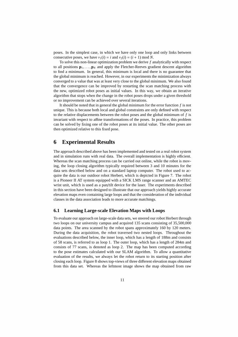
To evaluate our approach on large-scale data sets, we steered our robot Herbert throughtwo loops on our university campus and acquired 135 scans consisting of 35,500,000data points. The area scanned by the robot spans approximately 160 by 120 meters.During the data acquisition, the robot traversed two nestedloops. Throughout theevaluations described below, the inner loop, which has a length of 188m and consistsof 58 scans, is referred to as loop 1. The outer loop, which hasa length of 284m andconsists of 77 scans, is denoted as loop 2. The map has been computed accordingto the pose estimates calculated with our SLAM algorithm. Toallow a quantitativeevaluation of the results, we always let the robot return to its starting position afterclosing each loop. Figure 8 shows top-views of three different elevation maps obtainedfrom this data set. Whereas the leftmost image shows the map obtained from raw

11

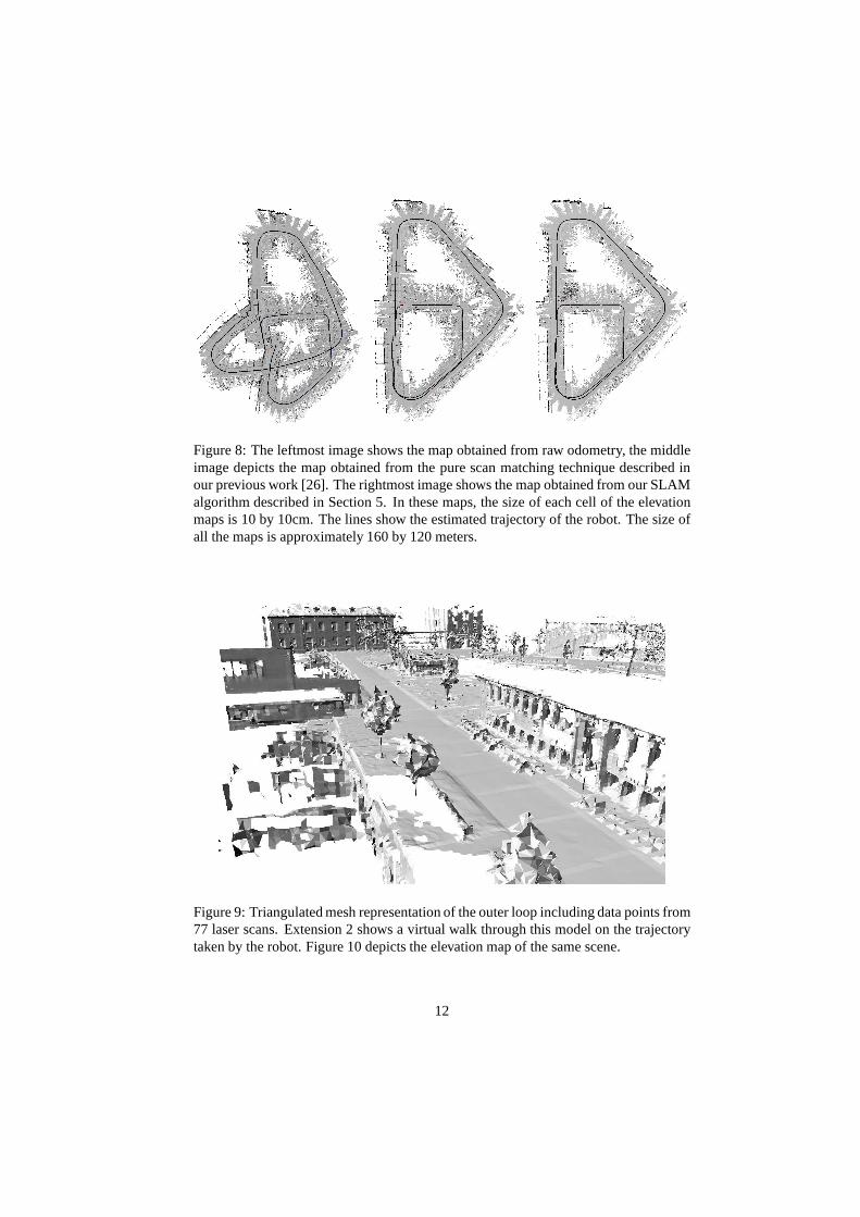
Figure 8: The leftmost image shows the map obtained from raw odometry, the middleimage depicts the map obtained from the pure scan matching technique described inour previous work [26]. The rightmost image shows the map obtained from our SLAMalgorithm described in Section 5. In these maps, the size of each cell of the elevationmaps is 10 by 10cm. The lines show the estimated trajectory ofthe robot. The size ofall the maps is approximately 160 by 120 meters.

Figure 9: Triangulated mesh representation of the outer loop including data points from77 laser scans. Extension 2 shows a virtual walk through thismodel on the trajectorytaken by the robot. Figure 10 depicts the elevation map of thesame scene.

12

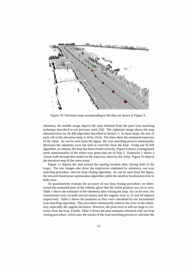
Figure 10: Elevation map corresponding to the data set shownin Figure 9.

odometry, the middle image depicts the map obtained from thepure scan matchingtechnique described in our previous work [26]. The rightmost image shows the mapobtained from our SLAM algorithm described in Section 5. In these maps, the size ofeach cell of the elevation maps is 10 by 10cm. The lines show the estimated trajectoryof the robot. As can be seen from the figure, the scan matching process substantiallydecreases the odometry error but fails to correctly close the loop. Using our SLAMalgorithm, in contrast, the loop has been closed correctly.Figure 9 shows a triangulatedmesh representation of the entire scan point data set of loop2. Extension 2 shows avirtual walk through this model on the trajectory taken by the robot. Figure 10 depictsthe elevation map of the same scene.

Figure 11 depicts the area around the starting location after closing both of theloops. The two images also show the trajectories estimated by odometry, our scanmatching procedure, and our loop closing algorithm. As can be seen from the figure,the network-based pose optimization algorithm yields the smallest localization error inboth cases.

To quantitatively evaluate the accuracy of our loop closingprocedure, we deter-mined the estimated pose of the vehicle, given that the initial position was set to zero.Table 1 shows the estimates of the odometry after closing theloop. As can be seen, thetranslational error exceeds several meters and the angularerror is 13 and 60 degreesrespectively. Table 2 shows the positions as they were calculated by our incrementalscan matching algorithm. This procedure substantially reduces the error in the odom-etry, especially the angular deviation. However, the pose error is still too large to cor-rectly close the loop. Finally, Table 3 shows the pose estimates obtained with our loopclosing procedure, which uses the results of the scan-matching process to calculate the

13

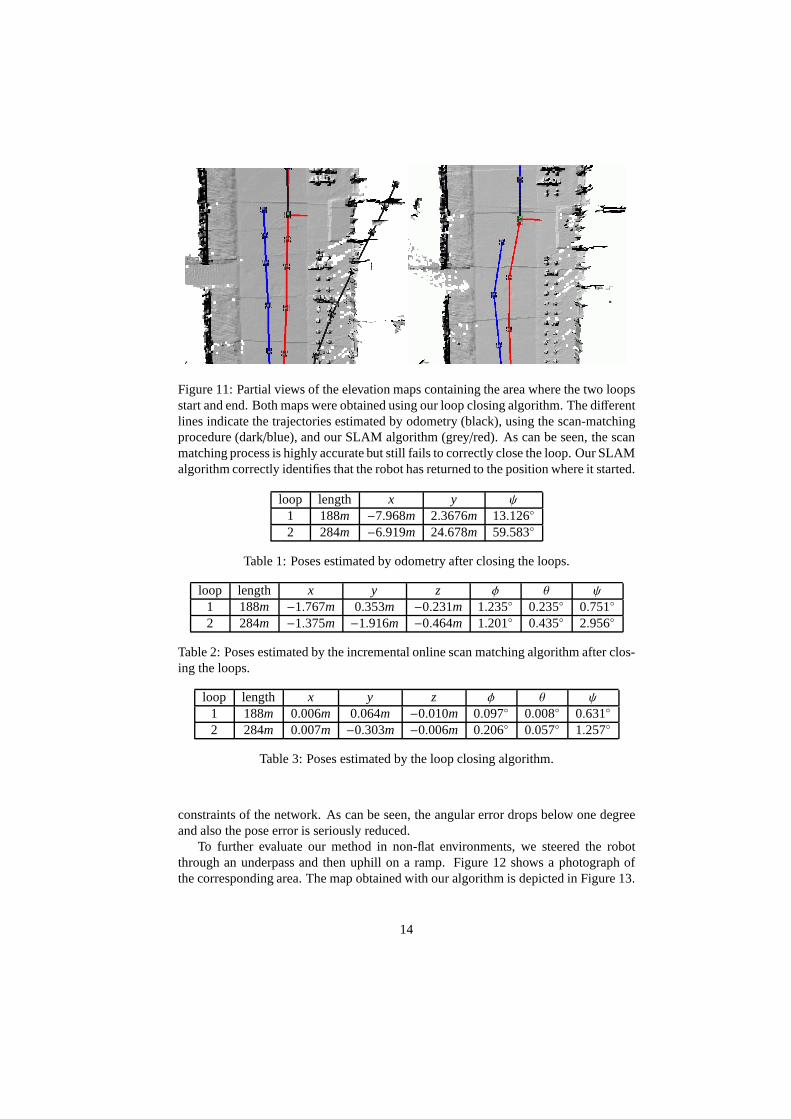
Figure 11: Partial views of the elevation maps containing the area where the two loopsstart and end. Both maps were obtained using our loop closingalgorithm. The differentlines indicate the trajectories estimated by odometry (black), using the scan-matchingprocedure (dark/blue), and our SLAM algorithm (grey/red). As can be seen, the scanmatching process is highly accurate but still fails to correctly close the loop. Our SLAMalgorithm correctly identifies that the robot has returned to the position where it started.

loop length x y ψ

1 188m −7.968m 2.3676m 13.126◦

2 284m −6.919m 24.678m 59.583◦

Table 1: Poses estimated by odometry after closing the loops.

loop length x y z φ θ ψ

1 188m −1.767m 0.353m −0.231m 1.235◦ 0.235◦ 0.751◦

2 284m −1.375m −1.916m −0.464m 1.201◦ 0.435◦ 2.956◦

Table 2: Poses estimated by the incremental online scan matching algorithm after clos-ing the loops.

loop length x y z φ θ ψ

1 188m 0.006m 0.064m −0.010m 0.097◦ 0.008◦ 0.631◦

2 284m 0.007m −0.303m −0.006m 0.206◦ 0.057◦ 1.257◦

Table 3: Poses estimated by the loop closing algorithm.

constraints of the network. As can be seen, the angular errordrops below one degreeand also the pose error is seriously reduced.

To further evaluate our method in non-flat environments, we steered the robotthrough an underpass and then uphill on a ramp. Figure 12 shows a photograph ofthe corresponding area. The map obtained with our algorithmis depicted in Figure 13.

14

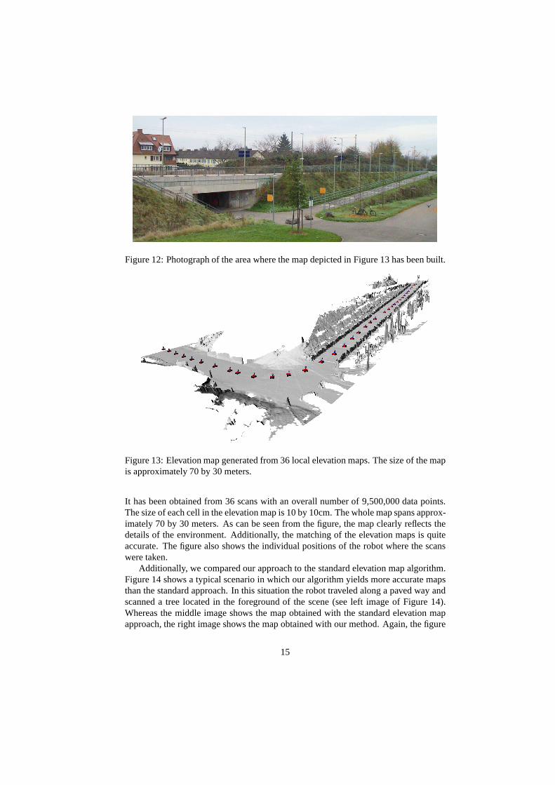
Figure 12: Photograph of the area where the map depicted in Figure 13 has been built.

Figure 13: Elevation map generated from 36 local elevation maps. The size of the mapis approximately 70 by 30 meters.

It has been obtained from 36 scans with an overall number of 9,500,000 data points.The size of each cell in the elevation map is 10 by 10cm. The whole map spans approx-imately 70 by 30 meters. As can be seen from the figure, the map clearly reflects thedetails of the environment. Additionally, the matching of the elevation maps is quiteaccurate. The figure also shows the individual positions of the robot where the scanswere taken.

Additionally, we compared our approach to the standard elevation map algorithm.Figure 14 shows a typical scenario in which our algorithm yields more accurate mapsthan the standard approach. In this situation the robot traveled along a paved way andscanned a tree located in the foreground of the scene (see left image of Figure 14).Whereas the middle image shows the map obtained with the standard elevation mapapproach, the right image shows the map obtained with our method. Again, the figure

15

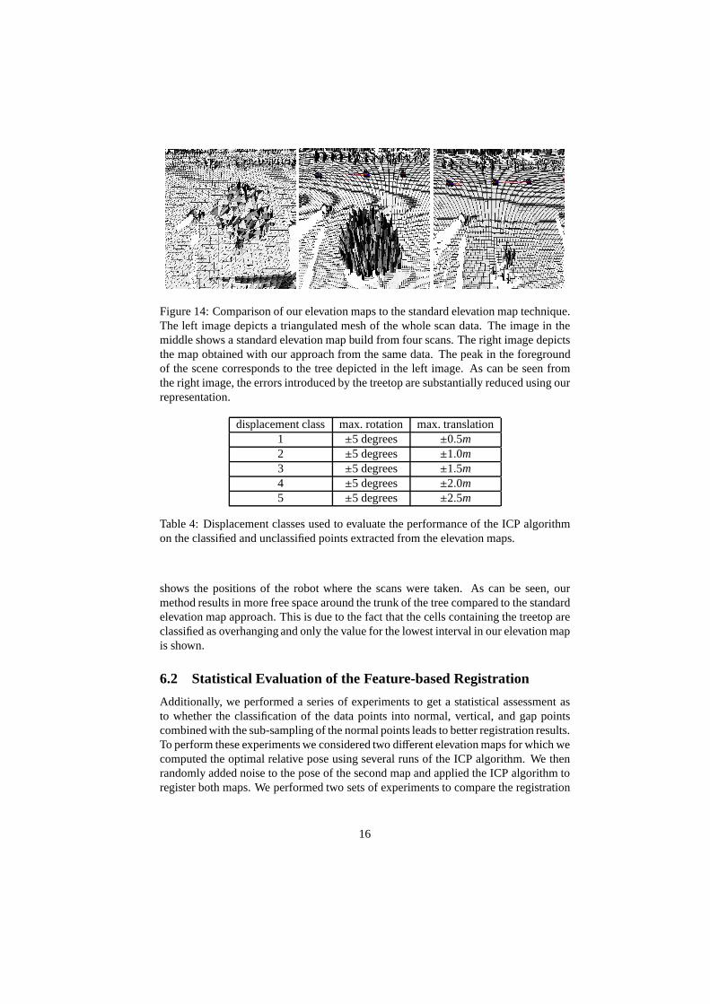
Figure 14: Comparison of our elevation maps to the standard elevation map technique.The left image depicts a triangulated mesh of the whole scan data. The image in themiddle shows a standard elevation map build from four scans.The right image depictsthe map obtained with our approach from the same data. The peak in the foregroundof the scene corresponds to the tree depicted in the left image. As can be seen fromthe right image, the errors introduced by the treetop are substantially reduced using ourrepresentation.

displacement class max. rotation max. translation1 ±5 degrees ±0.5m2 ±5 degrees ±1.0m3 ±5 degrees ±1.5m4 ±5 degrees ±2.0m5 ±5 degrees ±2.5m

Table 4: Displacement classes used to evaluate the performance of the ICP algorithmon the classified and unclassified points extracted from the elevation maps.

shows the positions of the robot where the scans were taken. As can be seen, ourmethod results in more free space around the trunk of the treecompared to the standardelevation map approach. This is due to the fact that the cellscontaining the treetop areclassified as overhanging and only the value for the lowest interval in our elevation mapis shown.

6.2 Statistical Evaluation of the Feature-based Registration

Additionally, we performed a series of experiments to get a statistical assessment asto whether the classification of the data points into normal,vertical, and gap pointscombined with the sub-sampling of the normal points leads tobetter registration results.To perform these experiments we considered two different elevation maps for which wecomputed the optimal relative pose using several runs of theICP algorithm. We thenrandomly added noise to the pose of the second map and appliedthe ICP algorithm toregister both maps. We performed two sets of experiments to compare the registration

16

0

0.05

0.1

0.15

0.2

0.25

0.3

0.35

0.4

1 2 3 4 5

aver

age

regi

stra

tion

erro

r

displacement class

classified pointsunclassified points

0

20

40

60

80

100

1 2 3 4 5

dive

rgen

ce fr

eque

ncy

[%]

displacement class

unclassified pointsclassified points

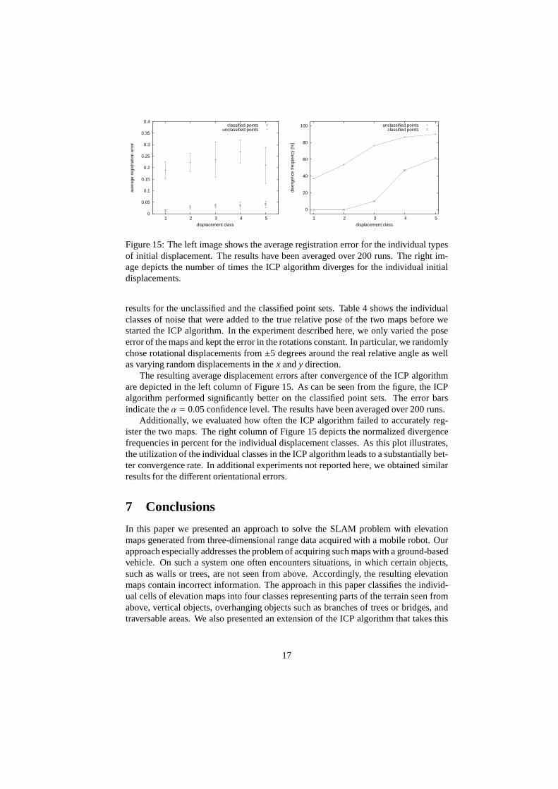
Figure 15: The left image shows the average registration error for the individual typesof initial displacement. The results have been averaged over 200 runs. The right im-age depicts the number of times the ICP algorithm diverges for the individual initialdisplacements.

results for the unclassified and the classified point sets. Table 4 shows the individualclasses of noise that were added to the true relative pose of the two maps before westarted the ICP algorithm. In the experiment described here, we only varied the poseerror of the maps and kept the error in the rotations constant. In particular, we randomlychose rotational displacements from±5 degrees around the real relative angle as wellas varying random displacements in thex andy direction.

The resulting average displacement errors after convergence of the ICP algorithmare depicted in the left column of Figure 15. As can be seen from the figure, the ICPalgorithm performed significantly better on the classified point sets. The error barsindicate theα = 0.05 confidence level. The results have been averaged over 200 runs.

Additionally, we evaluated how often the ICP algorithm failed to accurately reg-ister the two maps. The right column of Figure 15 depicts the normalized divergencefrequencies in percent for the individual displacement classes. As this plot illustrates,the utilization of the individual classes in the ICP algorithm leads to a substantially bet-ter convergence rate. In additional experiments not reported here, we obtained similarresults for the different orientational errors.

7 Conclusions

In this paper we presented an approach to solve the SLAM problem with elevationmaps generated from three-dimensional range data acquiredwith a mobile robot. Ourapproach especially addresses the problem of acquiring such maps with a ground-basedvehicle. On such a system one often encounters situations, in which certain objects,such as walls or trees, are not seen from above. Accordingly,the resulting elevationmaps contain incorrect information. The approach in this paper classifies the individ-ual cells of elevation maps into four classes representing parts of the terrain seen fromabove, vertical objects, overhanging objects such as branches of trees or bridges, andtraversable areas. We also presented an extension of the ICPalgorithm that takes this

17

classification into account when computing the registration. Additionally we use atechnique for constraint-based robot pose estimation to learn globally consistent eleva-tion maps.

Our algorithm has been implemented and tested on outdoor terrain data containingtwo loops. In practical experiments our constraint-based pose optimization yieldedhighly accurate maps. Additionally, the consideration of the individual classes duringthe data association in the ICP algorithm provides more robust correspondences andmore accurate alignments.

Acknowledgment

This work has partly been supported by the German Research Foundation (DFG) withinthe Research Training Group 1103 and under contract number SFB/TR-8.

A Index to Multimedia Extensions

The multimedia extensions to this article can be found online by following the hyper-links from www.ijrr.org.

Extension Type Description1 Video Incremental registration of two original point clouds2 Video Triangulated mesh representation of the outer loop in-

cluding data points from 77 laser scans. The exten-sion shows a virtual walk through this model on thetrajectory taken by the robot.

References

[1] P. Allen, I. Stamos, A. Gueorguiev, E. Gold, and P. Blaer.Avenue: Automatedsite modeling in urban environments. InProc. of the 3rd Conference on DigitalImaging and Modeling, pages 357–364, 2001.

[2] Peter K. Allen, Ioannis Stamos, Alejandro Troccoli, Benjamin Smith,M. Leordeanu, and Y. C. Hsu. 3D modeling of historic sites using range andimage data. InProc. of the IEEE Int. Conf. on Robotics& Automation (ICRA),Tapei, 2003.

[3] J. Bares, M. Hebert, T. Kanade, E. Krotkov, T. Mitchell, R. Simmons, andW. R. L. Whittaker. Ambler: An autonomous rover for planetary exploration.IEEE Computer Society Press, 22(6):18–22, 1989.

[4] P.J. Besl and N.D. McKay. A method for registration of 3-dshapes.IEEE Trans-actions on Pattern Analysis and Machine Intelligence, 14:239–256, 1992.

18

[5] A.J. Davison, Y. Gonzalez Cid, and N. Kita. Real-time 3d SLAM with wide-anglevision. In Proc. of the 5th IFAC Symposium on Intelligent Autonomous Vehicles(IAV), 2004.

[6] G. Dissanayake, P. Newman, S. Clark, H.F. Durrant-Whyte, and M. Csorba. A so-lution to the simultaneous localisation and map building (SLAM) problem. IEEETransactions on Robotics and Automation, 17(3):229–241, 2001.

[7] C. Fruh and A. Zakhor. An automated method for large-scale, ground-based citymodel acquisition.International Journal of Computer Vision, 60:5–24, 2004.

[8] J. Guivant and E. Nebot. Optimization of the simultaneous localization and mapbuilding algorithm for real time implementation.IEEE Transactions on Roboticsand Automation, 17(3):242–257, 2001.

[9] D. Hahnel, W. Burgard, and S. Thrun. Learning compact 3dmodels of indoor andoutdoor environments with a mobile robot.Robotics and Autonomous Systems,44(1):15–27, 2003.

[10] M. Hebert, C. Caillas, E. Krotkov, I.S. Kweon, and T. Kanade. Terrain mappingfor a roving planetary explorer. InProc. of the IEEE Int. Conf. on Robotics&Automation (ICRA), pages 997–1002, 1989.

[11] Daniel Huber and Martial Hebert. Fully automatic registration of multiple 3Ddata sets. InIEEE Computer Society Workshop on Computer Vision Beyond theVisible Spectrum(CVBVS 2001), December 2001.

[12] E. Hygounenc, I.-K. Jung, P. Soueres, and S. Lacroix. The autonomous blimpproject of laas-cnrs: Achievements in flight control and terrain mapping.Inter-national Journal of Robotics Research, 23(4-5):473–511, 2004.

[13] P. Kohlhepp, M. Walther, and P. Steinhaus. Schritthaltende 3D-Kartierung undLokalisierung fur mobile inspektionsroboter. In18. Fachgesprache AMS, 2003.In German.

[14] S. Lacroix, A. Mallet, D. Bonnafous, G. Bauzil, S. Fleury and; M. Herrb, andR. Chatila. Autonomous rover navigation on unknown terrains: Functions and in-tegration.International Journal of Robotics Research, 21(10-11):917–942, 2002.

[15] M. Levoy, K. Pulli, B. Curless, S. Rusinkiewicz, D. Koller, L. Pereira, M. Ginz-ton, S. Anderson, J. Davis, J. Ginsberg, J. Shade, and D. Fulk. The digitalmichelangelo project: 3D scanning of large statues. InProc. SIGGRAPH, pages131–144, 2000.

[16] Y. Liu, R. Emery, D. Chakrabarti, W. Burgard, and S. Thrun. Using EM to learn3D models with mobile robots. InProceedings of the International Conferenceon Machine Learning (ICML), 2001.

[17] F. Lu and E. Milios. Globally consistent range scan alignment for environmentmapping.Autonomous Robots, 4:333–349, 1997.

19

[18] C. Martin and S. Thrun. Online acquisition of compact volumetric maps withmobile robots. InIEEE International Conference on Robotics and Automation(ICRA), Washington, DC, 2002. ICRA.

[19] P.S. Maybeck. The Kalman filter: An introduction to concepts. InAutonomousRobot Vehicles. Springer Verlag, 1990.

[20] M. Montemerlo and S. Thrun. A multi-resolution pyramidfor outdoor robotterrain perception. InProc. of the National Conference on Artificial Intelligence(AAAI), 2004.

[21] H.P. Moravec. Robot spatial perception by stereoscopic vision and 3d evi-dence grids. Technical Report CMU-RI-TR-96-34, Carnegie Mellon University,Robotics Institute, 1996.

[22] A. Nuchter, K. Lingemann, J. Hertzberg, and H. Surmann. 6d SLAM with ap-proximate data association. InProc. of the 12th Int. Conference on AdvancedRobotics (ICAR), pages 242–249, 2005.

[23] C.F. Olson. Probabilistic self-localization for mobile robots.IEEE Transactionson Robotics and Automation, 16(1):55–66, 2000.

[24] C. Parra, R. Murrieta-Cid, M. Devy, and M. Briot. 3-d modelling and robotlocalization from visual and range data in natural scenes. In 1st InternationalConference on Computer Vision Systems (ICVS), number 1542 in LNCS, pages450–468, 1999.

[25] K. Pervolz, A. Nuchter, H. Surmann, and J. Hertzberg.Automatic reconstructionof colored 3d models. InProc. Robotik, 2004.

[26] P. Pfaff and W. Burgard. An efficient extension of elevation maps for outdoorterrain mapping. InProc. of the International Conference on Field and ServiceRobotics (FSR), pages 165–176, 2005.

[27] H. Samet.Applications of Spatial Data Structures. Addison-Wesley PublishingInc., 1989.

[28] S. Singh and A. Kelly. Robot planning in the space of feasible actions: Twoexamples. InProc. of the IEEE Int. Conf. on Robotics& Automation (ICRA),1996.

[29] S. Thrun, W. Burgard, and D. Fox. A real-time algorithm for mobile robot map-ping with applications to multi-robot and 3D mapping. InProc. of the IEEEInt. Conf. on Robotics& Automation (ICRA), 2000.

[30] S. Thrun, D. Hahnel, D. Ferguson, M. Montemerlo, R. Triebel, W. Burgard,C. Baker, Z. Omohundro, S. Thayer, and W. Whittaker. A systemfor volumetricrobotic mapping of abandoned mines. InProc. of the IEEE Int. Conf. on Robotics& Automation (ICRA), 2003.

20

[31] S. Thrun, Y. Liu, D. Koller, A.Y. Ng, Z. Ghahramani, and H. Durant-Whyte.Simultaneous localization and mapping with sparse extended information filters.International Journal of Robotics Research, 23(7-8):693–704, 2004.

[32] S. Thrun, C. Martin, Y. Liu, D. Hahnel, R. Emery Montemerlo, C. Deepayan, andW. Burgard. A real-time expectation maximization algorithm for acquiring multi-planar maps of indoor environments with mobile robots.IEEE Transactions onRobotics and Automation, 20(3):433–442, 2003.

[33] R. Triebel and W. Burgard. Improving simultaneous mapping and localizationin 3d using global constraints. InProc. of the National Conference on ArtificialIntelligence (AAAI), 2005.

[34] R. Triebel, F. Dellaert, and W. Burgard. Using hierarchical EM to extract planesfrom 3d range scans. InProc. of the IEEE Int. Conf. on Robotics& Automation(ICRA), 2005.

[35] Carl Wellington, Aaron Courville, and Anthony Stentz.Interacting markov ran-dom fields for simultaneous terrain modeling and obstacle detection. InProceed-ings of Robotics: Science and Systems, Cambridge, USA, June 2005.

[36] O. Wulf, K-A. Arras, H.I. Christensen, and B. Wagner. 2dmapping of clutteredindoor environments by means of 3d perception. InICRA-04, pages 4204–4209,New Orleans, apr 2004. IEEE.

[37] C. Ye and J. Borenstein. A new terrain mapping method formobile robot obsta-cle negotiation. InProc. of the UGV Technology Conference at the 2002 SPIEAeroSense Symposium, 1994.

21