Embed Size (px)
Citation preview
AN AVERAGE MODELING APPROACH OF HYBRID POWER SYSTEMS
FOR USE IN MOBILE REFRIGERATION APPLICATIONS
BY
YUE CAO
THESIS
Submitted in partial fulfillment of the requirements
for the degree of Master of Science in Electrical and Computer Engineering
in the Graduate College of the
University of Illinois at Urbana-Champaign, 2013
Urbana, Illinois
Adviser:
Professor Philip T. Krein

ii
ABSTRACT
This thesis presents averaging-based models of hybrid electric power systems for refrigeration
units in delivery trucks. The background of the mobile refrigeration industry is stated, and the
motivation of the proposed hybrid-powered ac motor drive is discussed. The model is intended to
be used for an industry power and energy flow study and eventually for a development of
product prototype. Challenges unique to this hybrid application, including the thermal system
interface, drive cycle response, and battery management, are introduced. The system topology is
presented, including the hybrid power architecture, electrical-thermal system specifications, and
the integrated model operation and controls. The modeling approach for each electrical
component, including ac machines, the battery set, and converters, is discussed. An average
modeling technique is used because it models system-level power and efficiency over a long
time interval with fast simulation. Battery simulation is improved from previous literature to
provide a more accurate and robust solution. The model, interfaced with the thermal system, is
verified by simulation studies in MATLAB/Simulink. A detailed model including transient
response and harmonics gives a more accurate reading for power loss, at the cost of a slower
simulation speed. It is not used directly for the industry study, but one detailed model is realized
in Simulink/SimPowerSystems to validate the average model. The average model is also
validated through experiments, including an active front end test, a battery test, and a variable
speed ac motor drive test. Using the model, energy and cost-effectiveness are analyzed and
discussed. Finally, the significance of the work is described and future improvements are
suggested.

iii
ACKNOWLEDGMENTS
This work was supported, in part, by Thermo King, a division of Ingersoll-Rand, and also by the
Power Affiliates Program at the University of Illinois – Urbana-Champaign.
This project would not have been possible without the support of many people. I would
like to give special thanks to my adviser, Prof. Philip Krein, for his guidance and support. His
broad knowledge in the power and energy systems area often surprises me and always charges
me with new thoughts and motivations. I also thank the coordinator of the Grainger Center for
Electric Machines and Electromechanics, Joyce Mast, for helping me improve the thesis content
through many revisions.
A special thanks to the project collaborators, including graduate student Joey Fasl and
Prof. Andrew Alleyne from the Department of Mechanical Science and Engineering, and Bill
Mohs, Petr Kadanik, and Casey Briscoe from Ingersoll-Rand.
I would also like to thank my graduate fellows Srikanthan Sridharan and Tutku
Buyukdegirmenci, and our lab manager, Kevin Colravy, who helped me with theory
development and the experimental set-up.
Last, I am most grateful to my mother, Rong Li, and my father, Tiechuan Cao, who have
always supported and loved me.

iv
TABLE OF CONTENTS
1 INTRODUCTION.......................................................................................................................1 1.1 Background ............................................................................................................................1
1.2 Motivation and Literature Review .........................................................................................6
1.3 Thesis Outline ........................................................................................................................9
2 SYSTEM OVERVIEW ............................................................................................................10
3 MODELING APPROACHES .................................................................................................15 3.1 Drive Cycle ..........................................................................................................................15
3.2 Induction Machine ................................................................................................................19
3.2.1 Induction machine power analysis .............................................................................19
3.2.2 Induction machine control ..........................................................................................21
3.2.3 Induction machine parameters calculation .................................................................23
3.3 Power Electronics Loss Modeling ........................................................................................26
3.3.1 Inverter .......................................................................................................................26
3.3.2 Converter ....................................................................................................................27
3.3.3 Rectifier ......................................................................................................................29
3.4 Generator ..............................................................................................................................31
3.5 Battery ..................................................................................................................................34
4 SIMULATION RESULTS .......................................................................................................39
4.1 Average Model Simulation ..................................................................................................40
4.2 Detailed Model Simulation ..................................................................................................49
5 EXPERIMENTAL VALIDATION .........................................................................................52
5.1 Front End Testing .................................................................................................................53
5.2 Battery Testing .....................................................................................................................56
5.3 Motor Drive Testing .............................................................................................................59
6 DISCUSSION ............................................................................................................................64
7 CONCLUSION AND FUTURE WORK ................................................................................69
REFERENCES .............................................................................................................................71
APPENDIX A SIMULINK MODELS .......................................................................................74
A.1 High-Level Integrated Thermo-Electric Model ..................................................................74
A.2 Average Model for Hybrid Power Systems ........................................................................74
A.3 Detailed Model for Hybrid Power Systems ........................................................................75
APPENDIX B MATLAB PROGRAMS ....................................................................................76
B.1 IM Parameters Calculation MATLAB Code .......................................................................76
B.2 PMSM Parameters Calculation MATLAB Code ................................................................77
1
1 INTRODUCTION
1.1 Background
The development of hybrid technologies helps to reduce emissions and increase fuel economy in
vehicles. In recent years, it has drawn researchers’ and industries’ attention to improve emissions
and energy consumption issues from heavy duty trucks during idling. Many of the trucks are
equipped with mobile refrigeration units (MRU) powered by auxiliary diesel engines. Figure 1.1
shows a typical produce delivery truck with an MRU. An airborne toxic and control measure
(ATCM) regulation has been proposed for MRU diesel engines to reduce particulate matter (PM)
emissions by 95% and nitrogen oxides (NOx) by 65% between 2004 and 2014 [1].
An MRU is a refrigeration system controlling the temperature in a truck shipping
container. It consists of a power unit which is usually a diesel engine, a refrigerant compressor, a
throttling valve, an evaporator, a condenser, fans for circulating the air over the heat exchangers
and a climate controller [2]. MRUs are used to deliver temperature sensitive products such as
Mobile refrigeration unit
Figure 1.1. A typical produce delivery truck with MRU
Source: FormerWMDriver on flickr.com

2
frozen, fresh or perishable food, medications, etc., from warehouse to market, and are usually
installed on midsize to large refrigerated trucks. The trucks can operate under a wide variety of
driving conditions, including high-speed limited-access highways or low-speed local streets,
mountainous terrains or flat country roads, and hot or cold ambient temperatures. Table 1.1
presents three possible scenarios. MRUs sometimes remain stationary for hours while loading
and unloading. Temperature is maintained by on/off engine cycling and loading/unloading the
MRU compressor.
Rural Suburban Urban
Miles per day 300 150 50
Stops per day 4 8-12 15-20
Length per stop (min) 25 15-20 10-15
Duration of doors open per stop (min) 10-15 5-10 <5
Total length of maintained temperature
required at stops (min) 40-60 80-200 100-250
Instead of trying to reduce emissions from the MRU diesel engine, it is preferred to
eliminate this diesel engine and seek an alternative power source. Given current hybrid
technology, this is possible. The compressor is driven by an electric machine, usually an ac
machine, which is powered and controlled by an ac motor drive. Hybrid power is applied to this
motor drive. There are a few considerations. MRUs must have sufficient refrigeration capacity to
maintain the desired set-point temperature, meet the cooling load demand and have fast pull-
down characteristics. Fast pull-down for a loaded truck is necessary to deal with frequent
Table 1.1. Delivery truck operating scenario examples

3
opening and closing of the container door. The cooling capacity for a typical truck container
varies between 3 and 9.3 kW [3]. When possible, MRUs can also have an option to plug in the
grid such as at loading docks. Commercial chargers can have three-phase 208 V, rated 50 A, and
up to 12 kW input power [4].
A hybrid power system requires power both from the truck’s main diesel engine and from
at least one other energy storage device. The latter can be a battery, a hydrogen fuel cell, a super
capacitor, etc., which supplies power to the motor drive and is also charged by the engine or
from the grid when necessary. Batteries are safe and stable power sources, and are relatively
inexpensive. However, they still face challenges such as the need for high energy density and
quick recharging rates. Lead-acid, nickel-metal hydride, molten salt, and lithium-ion battery
types can be used for transportation electrification purposes. Most electric vehicles (EVs),
including the Nissan Leaf and Tesla Motors S, utilize lithium-ion batteries because they allow
rapid charges as fast as a few minutes, and feature long life, fire resistance, and environmental
friendliness [5].
Variable speed drives (VSD) have significant implications for the efficient use of energy
for an MRU. Conventional unit-cycling and two-speed regulation methods for MRUs are
inefficient at controlling refrigeration capacity. Frequent starting and stopping of the compressor
leads to increasingly unsteady operation, high start-up power requirements, and high system
maintenance [3]. As the refrigeration system capacity is proportional to the compressor speed,
capacity control can be achieved by changing the compressor speed. Inverter based ac VSD are
used in many commercial and residential applications to achieve better control and energy
savings. However, in the MRU industry, diesel engine driven compressors still dominate, as
shown in Figure 1.2, and there is little VSD market penetration [1].

4
A hybrid-powered thermal-enhanced system architecture is proposed in Figure 1.3. On
the electrical engineering side, a hybrid power system model has been constructed utilizing a
generator, battery, variable frequency ac motor drive, and power electronics technology. On the
mechanical engineering side, an advanced controlled thermal system with thermal storage
options has been modeled. The power system and thermal system models are interfaced at the ac
machine and compressor junction. The combined model evaluates the hybridization system
architecture and controls strategy in regard to expected cooling duty cycles. Model-based
optimization criteria for performing control design tradeoffs, such as set-point maintenance vs.
energy consumed, will be addressed.
Condenser
Evaporator
W
TH
TLQL
QH
Figure 1.2. Conventional MRU electric-thermal operation diagram [6]

5
Figure 1.3. Proposed hybrid-powered thermal-enhanced system architecture [6]

6
1.2 Motivation and Literature Review
As mentioned earlier in this chapter, preventing pollution while a truck is idling is a strong
reason to use hybrid-powered MRUs. Because converting an MRU power system to hybrid
requires extra hardware and labor cost, one needs other incentives to make this change. HEVs
have proved to be more energy efficient than the conventional combustion engine vehicles [5].
One major energy-saving feature in HEVs is regenerative braking, meaning that the energy
generated from vehicle deceleration is stored in batteries instead of being wasted as heat [7]. The
stored energy is later used to power an electric motor for vehicle traction. However, in the MRU
case, the compressor has no deceleration region, making the regenerative braking feature
infeasible. Another energy saving point of interest is at diesel engine efficiencies. The medium to
heavy-duty truck main diesel engine has a higher efficiency than the light-duty compressor diesel
engine [8]. Becoming hybrid means that all the compressor energy comes from the main engine.
However, it should be noted that the hybrid power system, including electric machines and
power electronics that connect the truck engine and the compressor, is not lossless. Only if the
truck engine is significantly more efficient than the compressor engine, and the hybrid power
system is reasonably efficient itself, can the hybrid topology be an investment by industries and
customers.
The hybrid power system efficiency for a typical MRU is unknown. The recommended
approach is to model and simulate this system, and then to build a prototype for validation.
Commercial simulators such as Autonomie are suggested in [9]. Although these simulators have
well-refined component blocks for a hybrid power system, they are mostly used for HEV
applications and lack the possibility to integrate with the thermal system of an MRU. In [10-11],
recent development of VFDs in refrigeration systems is discussed. These papers describe

7
possible configurations for ac-grid powered systems as well as hybrid electric systems with ac
generators and batteries as the sources. Much emphasis has been placed on improvement for
controls to reduce total harmonic distortions and to improve efficiencies. A few also mention
industry standards and hardware implementation using VHDL/FPGA programmed digital signal
processors. However, few publications mention hybrid power systems for MRUs, particularly at
the system level and their modeling and simulation strategy. The differences between MRUs and
other refrigeration units include 1) frequent and drastic temperature changes due to loading and
unloading products, 2) variety of truck moving profiles depending on road conditions and
delivery schedules, and 3) availability of consistent and reliable power sources. Therefore, it is
necessary to build our own hybrid power system model in a suitable simulation tool and integrate
it with another thermal model that together can address the issues above. The models must be run
at the system level over extended periods of time because we are most interested in this hybrid
MRU topology’s practicality in the sense of system efficiency, and energy and cost savings.
In [12-14], various modeling and simulation methods for HEV power systems, including
machines and power electronics, are suggested. In particular, [15-18] provide modeling solutions
to lithium-ion batteries for hybrid electric systems. These electrical models are built in
MATLAB/Simulink, and the thermal model can be constructed in the same environment and
interfaced without extra effort. It should be noted that some of the modeling approaches are
intended for hardware design and include details such as machine transient dynamics and
semiconductor switching actions. As suggested by [19] these details in Simulink drastically
decrease the simulation speed and are not suitable for an efficiency study on a macro scope.
Hence the averaging modeling approaches solicited by [20] are necessary. With this philosophy
considered, electric machine steady-state equivalents by [21-22] and average loss calculation in

8
power semiconductors by [23] are implemented. In addition, a conversion from time-domain
differential equations to frequency-domain transfer functions for lithium-ion battery modeling in
[24-25] can be achieved. Therefore, a high-speed average model of hybrid power systems for
MRUs is expected. Efficiency and energy flow for MRUs over a long period can be obtained and
studied. Insightful energy and cost savings can be suggested to evaluate the hybrid system’s
performance and assist in decisions on whether or not a future development effort towards such a
system is meaningful.

9
1.3 Thesis Outline
This thesis is focused on system-level power and efficiency modeling based on fast simulation,
integrated with the refrigeration thermal system. The approach is defined as the average model in
subsequent chapters. A detailed dynamic model with transient analysis follows for validation
purpose and is called the detailed model for short. The challenges lie in integrating the
refrigeration system with an ac drive subsystem, responding to the dynamic drive cycle on the
alternator side, and managing batteries for unexpected thermal loadings, depending on whether
or not the truck is mobile. The average model can be easily integrated with the thermal system
model, because its simulation speed is comparable to that of the thermal system model, and it is
flexible to run at the user-desired time, power level, and drive cycle. It also provides a user-
friendly interface for easy modification of system parameters.
An overview of the hybrid power system configuration is presented in Chapter 2. Details
about the averaging modeling approaches are discussed in Chapter 3. In Chapter 4, power level
and efficiency results of each model component are achieved through successful simulation
based on reasonable assumptions as well as necessary machine, semiconductor device, and
battery parameters. A comprehensive simulation, integrating the hybrid power system and the
thermal system, is run against varying drive cycles and loading requirements. System dynamics,
including harmonics and complex variables, in addition to power and efficiency performance, are
also simulated from the detailed model. Chapter 5 describes the experimental set-up and
objectives. Relevant experimental data are presented and demonstrate the model’s accuracy.
Chapter 6 analyzes energy and cost-effectiveness using the average model for the MRU hybrid
power system.

10
2 SYSTEM OVERVIEW
A broad system configuration of a proposed hybrid MRU is depicted in Figure 2.1, and a
visualized system layout is shown in Figure 2.2. The system takes in power from the engine via a
direct-coupled generator, and also has the option to connect to the grid. A pack of lithium-ion
batteries also supplies power as a dc source. After power conversion and control, motor drives
operate compressors, fans, and blowers, comprising the thermal system. Heaters are also needed
to cover a full range of climate conditions. Figure 2.3 shows the hybrid power system: an engine
shaft drives an ac generator feeding a rectifier with a stabilized output dc bus; then a dc-ac
inverter connected to an ac induction machine drives the compressor; and the battery is in
parallel and connects at the dc bus. Notice that a dc-dc boost converter is required after the
rectifier because the rectifier output dc voltage is limited by the variable generator ac voltage. In
most cases the rectifier dc voltage is 200-500 V.
Power Supply System
Power electronics, switches & protection
Compressor
Control unit
Fans
Blowers
Heaters
Alternator
Standby
Commands & vehicle CAN Sensors
Unit battery
Grid
Aux loads
Hybrid Power System Engine/external Power Thermal System
Figure 2.1. System configuration of the proposed MRU
11
An ac machine rated up to 9 kW is selected based on previous industry experiences and
the typical industry cooling capacity for a truck container suggested by [3]. A three-phase 12 HP
460 V 60 Hz Y-connected ac induction machine (IM) is chosen (actual model withheld for
proprietary purpose). The machine can be configured as 230 V Y-connected; however, this
Lithium-ion battery
Engine and alternator
Power electronics and control units
Ac machine and compressor
Thermal systems
Figure 2.2. Physical layout of MRU major components, edited from [6]
AC Generator AC/DC Rectifier DC/DC Converter
DC Link
DC/AC Inverter Induction Motor
DC/DC Converter Battery Pack
Figure 2.3. Overall power system structure in the simulation model

12
doubles the system current, which results in more losses and thermal issues related to the IGBTs
and other electric components. An equivalently rated ac permanent magnet synchronous machine
(PMSM) is also suitable as the motor. Given the ac machine ratings, a dc bus voltage of 700 V is
deemed appropriate, and 1.2 kV IGBTs are suitable for all the power electronic devices. Energy
from a battery pack flows through a dc-dc boost converter before being connected to the dc bus.
The battery voltage can be in the 300-400 V range to maximize conversion efficiency. A three-
phase 17.3 kVA PMSM is chosen as the generator to be coupled with the engine.
The system model is built in MATLAB/Simulink. The goal of this hybrid system model
is to analyze long-term system and component response for practicality, hardware limitations,
efficiency, and fuel cost. It is most important to observe the power and efficiency at each
subsystem. Averaging and detailed modeling approaches are possible. For the average model,
simulation is carried out at the system level over a long time interval but must run quickly. It
simulates power changes and efficiency in equivalent steady-states at a fast simulation speed.
The model tolerates a wide range of sampling times up to 0.1 s to accommodate different thermal
or other electrical interfacing requirements. The detailed model is of higher-order dynamics that
include additional details, such as voltage/current transients and harmonics. However, its
simulation sampling time is a maximum 5 µs. For example, for a three-minute real-time
simulation run, the average model is able to simulate one hour of the system performance,
whereas the detailed model produces only two seconds of the model dynamics [20].
The average model strategy is chosen because it can be integrated with the thermal
system model, which has time steps of a few ms, and it is flexible to run at user-desired times,
power levels, and drive cycles. It also provides a user-friendly interface for easy modification of
system parameters. The approach is to model power losses in each subsystem (motor, converter,

13
battery, etc.), including conduction and switching devices loses, based on equivalent steady-state
conditions. Most losses have a direct relationship to the associated currents. Calculated output
currents from one subsystem are passed as input currents to the next subsystem. The power flow
can be examined in either direction, with input and output currents changing roles. For example,
current flowing into the induction machine can be calculated, given the output speed and torque
to the MRU compressor, and motor power loss can also be obtained. This induction machine
current then becomes the inverter output current. Machine mechanical losses must also be
included. These can be obtained from data sheets and basic tests.
A detailed dynamic model is still necessary and is constructed in Simulink/
SimPowerSystems. It serves as a validation check for the average model and is helpful for future
power electronic hardware design and implementation. The detailed model includes stepping
waveforms at each switching action from the semiconductor devices, with consideration of
snubber circuits. It also models the electric machines (PMSM, IM) as differential equations that
produce transient waveforms. Filters are also included between components, and harmonics
analysis can be performed.
Subsystem blocks shown in Figure 2.4 are based on the model structure in Figure 2.3.
The subsystems in the left column represent the engine-powered compressor drive, and those on
the upper right represent the battery powered compressor drive. Power level, battery state, and
efficiency observation are shown in the scopes.
14
The model can run based on the following scenarios: 1) Engine on, compressor on,
battery charging off; 2) engine on, compressor on, battery charging on; 3) engine on, compressor
off, battery charging on; 4) engine on, compressor off, battery charging off; 5) battery on,
compressor on; and 6) everything off. Notice that engine on and battery on are mutually
exclusive events. Users can define a critical engine RPM above which the engine is treated as on.
Similarly, the battery must be charged when the SOC (state of charge) is below a predefined
value. Signals from the thermal system will indicate when the compressor should be on.
The MATLAB/Simulink model can be run from any arbitrary time in the drive cycle and
can accept different initial states in each subsystem. It tolerates a wide range of sampling times
up to 0.1 s to accommodate different thermal or other electrical interfacing requirements.
Figure 2.4. Overview of subsystems in the hybrid power system model
15
3 MODELING APPROACHES
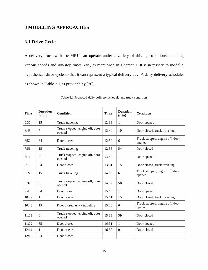
3.1 Drive Cycle
A delivery truck with the MRU can operate under a variety of driving conditions including
various speeds and run/stop times, etc., as mentioned in Chapter 1. It is necessary to model a
hypothetical drive cycle so that it can represent a typical delivery day. A daily delivery schedule,
as shown in Table 3.1, is provided by [26].
Time Duration
(min) Condition Time
Duration
(min) Condition
6:30 15 Truck traveling 12:39 1 Door opened
6:45 7 Truck stopped, engine off, door
opened 12:40 10 Door closed, truck traveling
6:52 64 Door closed 12:50 6 Truck stopped, engine off, door
opened
7:56 15 Truck traveling 12:56 54 Door closed
8:11 7 Truck stopped, engine off, door
opened 13:50 1 Door opened
8:18 64 Door closed 13:51 15 Door closed, truck traveling
9:22 15 Truck traveling 14:06 6 Truck stopped, engine off, door
opened
9:37 6 Truck stopped, engine off, door
opened 14:12 58 Door closed
9:43 64 Door closed 15:10 1 Door opened
10:47 1 Door opened 15:11 15 Door closed, truck traveling
10:48 15 Door closed, truck traveling 15:26 6 Truck stopped, engine off, door
opened
11:03 6 Truck stopped, engine off, door
opened 15:32 59 Door closed
11:09 65 Door closed 16:31 1 Door opened
12:14 1 Door opened 16:32 0 Door closed
12:15 24 Door closed
Table 3.1 Proposed daily delivery schedule and truck condition

16
The truck leaves the dispatch center at 6:30 in the morning and returns at 4:32 in the
afternoon. While the truck is running, it is commuting between delivery stations. After the truck
reaches a delivery location, the container door is opened to unload or load goods, and then
closed. It is important to maintain a required temperature inside the container. The door opening
and closing event has a drastic impact on the internal temperature. This sudden cooling cycle
change can impose an immediate high power demand from the electric system. During modeling
and simulation, the thermal system demand is reflected in the increase of compressor speed and
torque. The IM and the rest of the electric system must respond quickly to the change, and hence
generate new power and efficiency profiles.
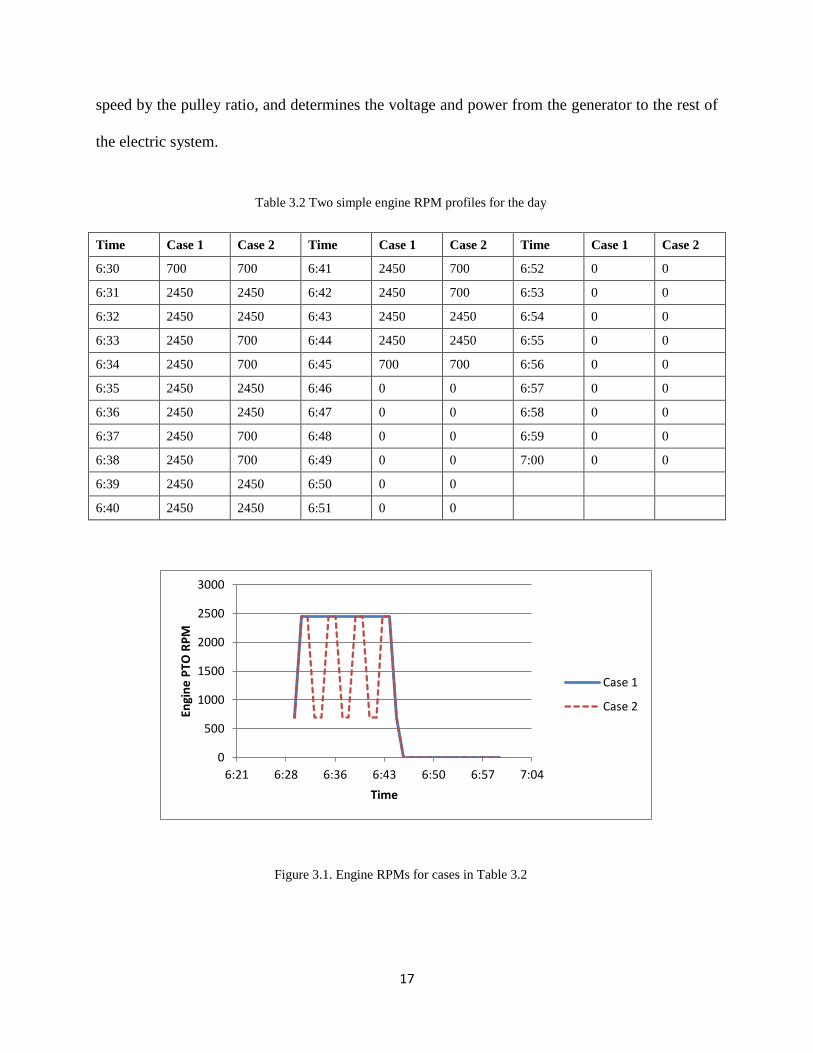
When the truck engine is running, it has varying power takeoff (PTO) speeds, with a
minimum of 700 RPM and a maximum of 2450 RPM [8]. The electric generator, direct-coupled
with the truck engine, has a pulley ratio of 2.06, and therefore, the minimum generator RPM is
1442 and maximum is 5047. Table 3.2 presents two simple hypothetical cases of how the engine
PTO speeds vary during delivery condition associated with Table 3.1. Figure 3.1 is the graph
depicting the data in Table 3.2.
The above cases give an idea what a drive cycle behaves like, but they are far less
sophisticated and realistic. Drive cycle data from actual driving conditions are found from an
industry vehicle battery validation study [27]. For the study, a test vehicle was run through
several drive cycles to gather actual RPM, temperature, and battery current and voltage data to
compare to the simulation. Figure 3.2 shows the first 20 minutes of the drive cycle after adjusting
the original data scales for both RPM’s and times. The truck engine speed varies during the first
15 minutes, and stops while the door is open. The same dynamic is repeated throughout the rest
of the day, as shown in Figure 3.3. The drive cycle profile directly guides the generator running
17
speed by the pulley ratio, and determines the voltage and power from the generator to the rest of
the electric system.
Time Case 1 Case 2 Time Case 1 Case 2 Time Case 1 Case 2
6:30 700 700 6:41 2450 700 6:52 0 0
6:31 2450 2450 6:42 2450 700 6:53 0 0
6:32 2450 2450 6:43 2450 2450 6:54 0 0
6:33 2450 700 6:44 2450 2450 6:55 0 0
6:34 2450 700 6:45 700 700 6:56 0 0
6:35 2450 2450 6:46 0 0 6:57 0 0
6:36 2450 2450 6:47 0 0 6:58 0 0
6:37 2450 700 6:48 0 0 6:59 0 0
6:38 2450 700 6:49 0 0 7:00 0 0
6:39 2450 2450 6:50 0 0
6:40 2450 2450 6:51 0 0
0
500
1000
1500
2000
2500
3000
6:21 6:28 6:36 6:43 6:50 6:57 7:04
Engi
ne
PTO
RP
M
Time
Case 1
Case 2
Table 3.2 Two simple engine RPM profiles for the day
Figure 3.1. Engine RPMs for cases in Table 3.2

18
Figure 3.2. Realistic engine RPMs for the first 20 min [8]
Figure 3.3. Realistic engine RPMs for a day [8]

19
3.2 Induction Machine
3.2.1 Induction machine power analysis
The IM is the direct interface with the thermal system. It is coupled with the compressor and
responds to the thermal system speed and torque demands. Not only is the IM power analysis
important, but also the IM control is crucial to respond robustly and efficiently.
For efficiency performance, to calculate the losses inside the machine, we first find the
required output power and calculate the input voltage, current, and power factor, which lead to
the total input power. The output power follows equation
TP outIM _ (3.1)
with the rotational speed and torque desired by the thermal system. There is a 1.6 pulley ratio
between the IM and the compressor. Note that the mechanical loss between the power and
thermal systems is not included, as there is no readily data available.
Circuit analysis must be performed for each phase of the IM in order to find the input
voltage, current, and power factor. Assuming the IM is three-phase balanced, the per-phase
equivalent steady-state circuit can be used as in Figure 3.4 [21]. The power flow is based on one
phase of the IM.
Figure 3.4. Equivalent steady state per phase circuit model of IM

20
The rotor series branch current is calculated based on
s
sRIP outIM
13 2
22_ (3.2)
s
s
R
PI
outIM
13 2
_
2 (3.3)
where s is the machine slip. The slip calculation will be discussed more in Section 3.2.2. I2 is the
RMS current magnitude in the rotor branch. Taking this current as the reference, I2 has an angle
equal to zero. Hence the voltage across the shunt branch is
)21
(0 22222 fLjs
RIV o (3.4)
The current flowing through the shunt branch can be calculated as
cm
mmR
V
fLj
VI 2222
2
(3.5)
Therefore, the current flowing through the stator series branch, or the IM input current, can be
calculated as
o
mmI III 0211 (3.6)
Hence the total per-phase input voltage across the IM is
22111111 )2( VfLjRIV IV (3.7)

21
Finally, with the per-phase input voltage and current, the total three-phase input power can be
calculated in equation
)Re(3 1111 IVIM IVP (3.8)
3.2.2 Induction machine control
The IM is to be controlled by the VSD methodology. The advantages of VSD ac motor drives
include reduced energy consumption, smooth transient voltage and current waveforms, and little
maintenance with long equipment life. Most commonly offered VSD control techniques are
volts-per-hertz (V/f) control, field oriented control, direct torque control, etc. Each has its pros
and cons. For this mobile refrigeration application, given that the IM is driving the compressor to
maintain a certain range of thermal flow inside the truck storage body, no complicated and
precise control is necessary, and the reduction of production cost is relatively more important. In
this sense, a V/f control is chosen [22]. Figure 3.5 illustrates this control technique.
Compressor
/Fan model
Slip
computation
Ac motor
drive
Motor
model
Speed
torque
Frequency
voltage
Speed
torque
PWM
waveform
Figure 3.5. IM V/f control diagram

22
The inputs are speed and torque references from the thermal system. The outputs are
controlled stator voltage, input frequency, and slip. The stator voltage and slip can be expressed
in terms of the frequency, as shown in equations
60
3/460
f
Vstator or fVstator60
3/460 (3.9)
pf
n
n
ns
ref
sync
ref
/12011 or
)1(120 s
pnf
ref
(3.10)
where f is the frequency in Hz, p is the number of poles, and s is the slip. The slip calculation
subsystem which implements the Simulink built-in algebraic constraint block essentially solves
0 refcalc TT (3.11)
where Tcalc is the calculated torque based on an initial slip estimate, usually about 0.02, and Tref is
the desired torque output. The algebraic constraint block produces the slip by forcing the two
torque values to be equal via feedback PI control. Then the input frequency and voltage values
are eventually known from (3.9) and (3.10). The calculated torque is based on
s
calc
sRIT
)/(3 222 (3.12)
which is the same as
221
221
212
)())/((
)/(3
XXsRR
VsRT
eqeq
eq
s
calc
(3.13)
23
in which I2 is replaced by a series of calculation using the Thevenin equivalent circuit from
Figure 3.4, and ωs is the synchronous speed in rad/sec. V1eq, R1eq, and X1eq are solved by [21]
)()||(
)||(
11
1jXRRjX
RjXVV
cm
cmstatoreq
(3.14)
)()||(
))(||(
11
11111
jXRRjX
jXRRjXZjXR
cm
cmeqeqeq
(3.15)
A quick check to see if the system works is to verify if the Vstator value (3.9) and V1 value (3.7) in
the IM system are equal.
3.2.3 Induction machine parameters calculation
In industry, engineers are usually provided with machine data sheets, which include the
following values: rated voltage, rated frequency, locked rotor current, locked rotor torque,
number of poles, power factor at rated frequency, efficiency at rated frequency, rated horse
power at rated frequency, and rated RPM at rated frequency. These data sheets can be used to
derive the equivalent stator/rotor resistance (R1, R2) and leakage inductance (L1, L2) as well as
copper resistance (Rc) and magnetizing inductance (Xm), given the IM per-phase equivalent
circuit (Figure 3.4).
The impedances, at two different frequencies, given in
|)(2)(||| 211211 LLfjRRZ f (3.16)
24
|)(2)(||| 212212 LLfjRRZ f (3.17)
can be found from the locked rotor test in
locked
ratedf
I
VZ
3/|| (3.18)
Then L1 and L2 can be found from equation
22
21
2
2
2
1
2121)2()2(2
1)(
2
1
ff
ZZLLLL
ff
(3.19)
where L1 and L2 are assumed to be equal. The rotor resistance R2 can be measured from a locked
rotor test when slip s is equal to 1. Equation
sRIP locked
13 2
2 (3.20)
defines the air gap power, and equation
]2
/)2/[(1
3 22 pole
fs
RIT elocked (3.21)
defines the torque from (3.20) [21]. The locked torque is given in the data sheets. R1 then can be
found from a derivation of (3.16) or (3.17).
Now we will determine Rc and Lm in the shunt branch. The main idea is to find the
impedance of Rc and Lm, or actually easier, the admittance. The admittance can be found if the
shunt branch voltage and current are known. Shunt voltage can be realized from equations

25
)2(3/ 111 fLjRIVV ratedshunt (3.22)
)arccos(3/
3///746|| 111 PF
V
PFeffHPII
rated
(3.23)
Shunt current can be realized from
22
1212/ fLjsR
VIIII shunt
shunt
(3.24)
Lm and Rc are found from
mc
shuntshuntshuntfLjR
VIY2
11/ (3.25)
The IM datasheet and the MATLAB code for the machine parameter calculation are in the
appendix.

26
3.3 Power Electronics Loss Modeling
3.3.1 Inverter
The inverter power losses can be found once the induction machine input power (PIM) and line
currents (Irms_IM) are calculated. The total inverter loss consists of conduction and switching
losses in IGBTs.
Figure 3.6. dc-ac inverter circuit diagram
The dc-ac inverter is modeled as three-phase full H-bridge with 6 IGBTs, as shown in
Figure 3.6. The conduction loss is incurred when the IGBT is turned on. It can be modeled as an
ideal switch in series with a forward voltage drop (Von) and a series resistor (Rds), as shown in
Figure 3.7. Von and Rds can be obtained directly from the IGBT datasheet. For this project, 1.2 kV
IGBTs are chosen.
Figure 3.7. Circuit model of a semiconductor device

27
The average conduction loss per IGBT pair is calculated in equation [23]
dsIMrms
onIMrms
invon RIVI
P 2_
_
_
22
(3.26)
and then multiplied by three for a three-phase circuit. The average switching loss of each IGBT
pair is calculated by [23]
2
22_
_
_
offon
invswitch
busIMrms
invswitch
ttf
VIP
(3.27)
where fswitch_inv is the 10 kHz inverter switching frequency. Times ton and toff are the switching
rise and fall times, respectively, which are also found in device datasheet. Vbus is the 700 V main
dc bus voltage. The loss again is multiplied by three for a three-phase circuit.
Thus, the total power into the dc-ac inverter is summarized in
invswitchinvonIMinv PPPP __ 33 (3.28)
3.3.2 Converter
A dc-dc converter is used between the rectifier and the dc bus, and one is also used between the
battery and the dc bus. The modeling approach is the same for both converters. A boost converter
between the rectifier and the dc bus is shown in Figure 3.8. The power loss consists of the IGBT
and diode conduction losses and the IGBT switching losses.
The converter duty ratio must be known to find the losses. It is calculated based on

28
convinconvout
convinconvout
convout
convinconvout
VV
VV
V
VVD
__
__
_
__ 1
(3.29)
where Vout_conv is 700 V, the same as the dc bus voltage, and Vin_conv is the dc voltage to be
computed in Section 3.3.3 from the rectifier (Vout_rect). The rearrangement of terms in (3.29)
simplifies some Simulink work. A lower limit is set for Vin_conv so that if the input voltage is too
low, the duty cycle is set to be zero.
Fig. 3.8. Boost converter circuit diagram
The converter conduction loss, like the inverter conduction loss, can be modeled using
Figure 3.7 (Section 3.3.1). It is based on
dsconvLonconvLIGBTConvon RDIVDIP 2___ (3.30)
where IL_conv is the converter input current, D is the duty cycle, Von is the IGBT forward voltage,
and Rds is the IGBT series resistance. Given Vin_conv, IL_conv is calculated after Pconv, the total
converter input power, is found with all the losses included. This may create a potential algebraic
loop in Simulink, since IL_conv is also required to calculate Pin_conv. To avoid this, a sampling
delay time is inserted in Simulink for the IL_conv calculation. The diode conduction loss is similar
except that the diode is turned on during the 1-D cycle, and it is only modeled as a forward
voltage drop in series with an ideal switch, as shown in

29
diodeonconvLDiodeConvon VIDP ___ )1( (3.31)
The average IGBT switching loss is found using equation [23]
convLconvout
offon
convswitchconvswitch DIVtt
fP ____2
(3.32)
where fswitch_conv is the 10 kHz switching frequency, ton and toff are the switching rise and fall
times in the device, and Vout_conv is the same as the main dc bus voltage.
Therefore, the total power into the dc-dc converter is summarized in
convswitchDiodeConvonIGBTConvonbattinvconv PPPPPP ___ (3.33)
where Pinv and Pbatt are the power flowing to the dc-ac inverter and battery charger, respectively.
3.3.3 Rectifier
The ac-dc rectifier topology is like the dc-ac inverter, but flipped horizontally, as shown in
Figure 3.9. Hence the power loss calculation is similar. The average conduction loss per IGBT
switch pair is shown in equation [23]
dsPMSMa
onPMSMa
recton RIVI
P 2_
_
_
22
(3.34)
where Ia_PMSM is the line RMS current out of the PMSM ac generator. Ia_PMSM is calculated in
Section 3.4.

30
The average switching loss of each IGBT switch pair is found using [23]
2
22_
__
_
offon
rectswitch
rectoutPMSMa
rectswitch
ttf
VIP
(3.35)
where fswitch_rect is the 10 kHz switching frequency, and Vout_rect is the rectified output dc voltage.
Vout_rect can be controlled to vary up to the maximum, which is limited by the generator line-line
voltage. Given the generator voltage range in Table 3.3 in Section 3.4, it is reasonable for this
average model to fix Vout_rect at a particular value, as in equation
PMSMtrectout VV __
332
(3.36)
based on a passive rectifier topology, which is only directly proportional to the PMSM terminal
voltage [23]. Under typical drive cycle Vout_rect yields an efficient 200-500 V for the boost
converter input voltage, knowing that the converter output voltage is 700 V dc bus.
Figure 3.9. ac-dc rectifier circuit diagram
Therefore, the total power going into the ac-dc rectifier is summarized in
rectswitchrectonconvrect PPPP __ 33 (3.37)
31
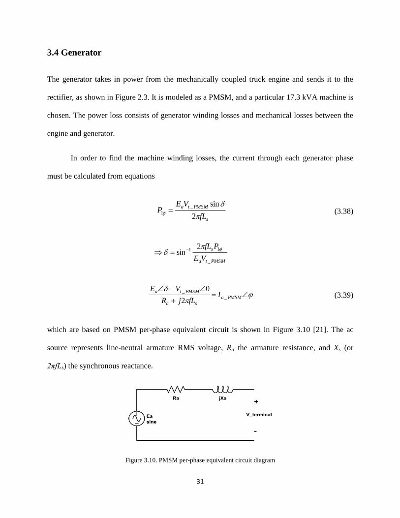
3.4 Generator
The generator takes in power from the mechanically coupled truck engine and sends it to the
rectifier, as shown in Figure 2.3. It is modeled as a PMSM, and a particular 17.3 kVA machine is
chosen. The power loss consists of generator winding losses and mechanical losses between the
engine and generator.
In order to find the machine winding losses, the current through each generator phase
must be calculated from equations
s
PMSMta
fL
VEP
2
sin_
1 (3.38)
PMSMta
s
VE
PfL
_
112
sin
PMSMa
sa
PMSMtaI
fLjR
VE_
_
2
0 (3.39)
which are based on PMSM per-phase equivalent circuit is shown in Figure 3.10 [21]. The ac
source represents line-neutral armature RMS voltage, Ra the armature resistance, and Xs (or
2πfLs) the synchronous reactance.
Figure 3.10. PMSM per-phase equivalent circuit diagram

32
P1φ is the per-phase output power, which is one third of the known power into the rectifier, Prect.
Ea is the armature voltage (line-neutral RMS) calculated by
kEa (3.40)
where k is a constant and ω is the rotational speed in thousands RPM.
Table 3.3. Data sheet for a selected PMSM
The generator RPM value is directly proportional to the drive-cycle controlled engine
RPM, with a 2.06 pulley ratio. k, in volts (line-neutral RMS) per 1000 RPM, is realized by
dividing the fourth column in by the first column in Table 3.3, a testing datasheet for a selected
PMSM (actual machine model withheld for proprietary purpose). The relationship between these
two columns is linear. Note that the values in column 4 are in line-line RMS, which is √ times
the line-neutral RMS. Due to engine RPM limit, generator speeds are only used up to 5000 RPM.
It is reasonable to assume that the terminal voltage magnitude (Vt_PMSM) is the same as the
armature voltage magnitude (Ea), but the phase angles are different. The PMSM frequency, f, can
be calculated by a frequency constant multiplied by the rotational speed; the relationship is linear.

33
The frequency constant, in Hz per 1000 RPM, is realized from columns 1 and 2 of Table 3.3. Ra
and Ls are obtained from simple machine tests, and they are 0.5 Ω and 2 mH, respectively. The
current magnitude is only required for power loss calculation, as shown in
aPMSMaPMSMloss RIP2
__ 3 (3.41)
In which the current angle, φ, is not used.
There is another loss in the system, mechanical loss, which is represented in the last
column of Table 3.3. It is interpolated as a quadratic function of RPM. This function is shown in
RPMRPMP PMSMmech 011022.0105.0459 2-5
_ (3.42)
which has a 0.99 coefficient of determination (R2).
Therefore, the total generator input power is summarized in
PMSMmechPMSMlossrectPMWM PPPP __ (3.43)
Note that this power is also the overall system input power.

34
3.5 Battery
The battery model is the key to the hybrid power system. An accurate and efficient model is
required to estimate battery instantaneous conditions and to interface properly with other models
in the power system. The battery model consists of four blocks, Battery Cell, SOC, Battery
Power Loss, and Power Battery. They calculate individual battery cell voltages, instantaneous
state of charge (SOC) in each battery cell, instantaneous power losses through all the battery
cells as well as total energy losses throughout a simulation cycle, and total power into/out of all
the battery cells, respectively. An additional block controls the battery (dis)charge rate, based on
running conditions in the overall system. The completed battery model enables a user to pre-
program a critical charging SOC value, a desired charging current, numbers of parallel and series
connected battery cells. Note that the battery models for the discharging stage and the charging
stage are built separately. The principle is the same, but the parameters are mostly different.
The Battery Cell block is modeled as the circuit in Figure 3.11 [24]. The second, minute,
and hour based resistors and capacitors predict battery cell behavior in each of the corresponding
time frames. The terminal voltage is calculated in
)1
||1
||1
||(th
th
tm
tm
ts
tsseriescoctsC
RsC
RsC
RRIVV (3.44)
Each parallel RC pair equivalent impedance is calculated in
sRC
sR
sCR
sCR
sCR
/1
/
/1
/1||
(3.45)

35
The rearrangement of equations in (3.45) simplifies the block construction in Simulink. The
modeling technique in [25] uses differential equations in the time domain. However, the
frequency domain method used in (3.44) proves to be equally functional and more efficient.
The voltage source, resistors, and capacitors depend non-linearly on the battery SOC. In
[24], V, C, and R values are modeled as 6th
order polynomials of SOC. Upon simulation using the
parameters from [25], some polynomial curves can become negative, which creates instability.
Also the coefficients of determination (R2) of the 6
th order polynomials with respect to the
measured samples are poor (Figure 3.12). In [15], it suggests various ways to curve fit data
points for battery modeling. In the proposed interpolation equations
6
0
66
2210 )(ln)(ln...)(ln)ln(),,ln(
k
kk SOCaSOCaSOCaSOCaaRCV (3.46)
])(lnexp[,,6
0
k
kk SOCaRCV (3.47)
R2 is a minimum of 0.8. One fitting curve is also plotted in Figure 3.12 to compare with the
original curve. The new method produces more accurate V, C, R values and thereby models the
battery more robustly.
Figure 3.11. Electrical battery model circuit

36
Table 3.4. Coefficients for functions used in Figure 3.11
a0 a1 a2 a3 a4 a5 a6
Voc 1.4222 0.2214 0.1829 0.0745 0.0145 0.0014 5×10⁻⁵
Rseries (D) -2.9384 -0.2328 -0.2109 -0.1294 -0.0302 0 0
R_s (D) -3.4883 -1.2434 -0.5619 0.0044 0.0348 0 0
C_s (D) -0.146 0.3731 1.6511 1.0513 0.1918 0 0
R_m (D) -3.1892 -0.0486 1.4851 6.1491 7.0124 3.1645 0.4997
C_m (D) 6.9413 -6.5951 -29.577 -56.356 -46.582 -16.991 -2.2588
Rseries (C) -2.8108 0.6011 0.8951 0.436 0.07 0 0
R_s (C) -3.5637 0.0016 3.4633 4.6412 2.2718 0.425 0.0188
C_s (C) -0.2737 -3.4945 -14.705 -21.767 -14.113 -4.1803 -0.4632
R_m (C) -2.8744 1.1014 1.1243 0.266 -0.1345 -0.046 0
C_m (C) 6.9622 -0.447 2.896 4.5575 2.2427 0.3544 0
R_h -5.6352 5.1517 12.006 6.1973 0 0 0
C_h 14.622 -6.2451 -19.818 -11.446 0 0 0
The new coefficients of (3.46) are listed in Table 3.4. (C) and (D) indicate the
coefficients for the charging and the discharging stages, respectively. Single-cell data (current,
SOC) are extracted from precise measurements of Panasonic CGR18650A 3.7 V, 2200 mAh Li-
Figure 3.12. Improved curve fitting and original [25] curve fitting for R_min constant
Proposed curve fitting
--------- Original curve fitting
Measured Rm values

37
ion batteries [25]. The same curve fitting strategy can be applied to other battery types. Second,
minute, and hour constants are tested with respect to SOC, and details regarding the testing are
found in [25].
The SOC block is modeled based on
dttitifdttitifSOCtSOC edisch
t
edischech
t
echinitial )()]([)()]([)( arg
0
arg2arg
0
arg1 (3.48)
where the initial SOC is constant and defined prior to simulation, i(t) is the instantaneous
discharging or charging current through each battery cell, and f is a function of that current and
modeled as a 1-D lookup table. The relationships between f and i are given in Tables 3.5 and 3.6
for the charging and discharging stages [25]. The SOC function (3.48) is a combination of
mentioned equations in [24]. The advantage is to reduce control effort and improve system
monitoring.
Table 3.5. f and i relationship for the charging stage.
i (charge) 0 0.0838 0.4386 1.0988 2.202
f(i) 1.34×10⁻⁴
1.3259×10⁻⁴
1.2581×10⁻⁴
1.2391×10⁻⁴
1.2192×10⁻⁴
Table 3.6. f and i relationship for the discharging stage.
i (discharge) 0 0.0808 0.4389 1.0886 2.1603
f(i) -1.4×10⁻⁴
-1.3751×10⁻⁴
-1.2727×10⁻⁴
-1.3222×10⁻⁴
-1.3928×10⁻⁴

38
Following the circuit diagram in Figure 3.11, the Battery Power Loss block is
straightforward, as the power loss through Rseries is I2R, and losses through Rs, Rm, Rh, are V
2/R.
The sum of power losses in each cell is the battery package power loss. Total energy loss is the
integration of all the power losses.
The charging power in the Power Battery block is the terminal voltage multiplied by the
branch current, VI, then multiplied by the total number of cells. Note that for the discharging
stage the total power consuming from the battery pack is this terminal power plus the total power
loss as calculated in the Battery Power Loss block, as the current is going outwards.
Dc-dc converters are required between the battery package and the system main dc bus.
These converter models are similar to those discussed earlier in the Section 3.3.2. Note that the
discharging stage converter is a boost converter, and the charging stage a buck converter. One
difference between the battery converter models is the duty cycle calculation. For the boost
converter, it is (1 - Vbattery/Vdc_bus), and for the buck converter Vbattery/Vdc_bus.

39
4 SIMULATION RESULTS
A comprehensive simulation must be run for the integrated thermal-electrical system. It is
important to evaluate each electrical component’s performance under a real-life scenario. The
scenario includes both the run/stop drive cycle as described in Section 3.1, and the dynamic
thermal loading demand based on the desired truck container temperature, ambient temperature,
door open/close events, etc. Figure 4.1 illustrates the system architecture. The power system
model is commanded by the engine RPM that is tied to the generator (PMSM), and is controlled
by the torque and speed references from the thermal system. The thermal system model receives
power from the motor (IM) and supplies required cooling/heating capacity in the form of
discharged air to the box (container) model, after compressing the returned air from the
container.
PowerSystem Model
Thermal System Model
Box Model
Control Model
DischargeAir
Sensor Feedback
Control
Control
Return Air
PowerTransfer
Engine RPM
Figure 4.1. MRU thermal-electric architecture for simulation integration

40
4.1 Average Model Simulation
The integrated system is simulated from 20,000 s to 29,000 s, which corresponds to 1:00 PM to
3:30 PM of the delivery schedule in Table 3.1. Figure 4.2 shows the engine and generator RPMs
and serves as the drive cycle reference. There are several noteworthy events: container door
opens (Figure 4.3), motor drives the compressor (Figure 4.4), and battery is charged and
discharged (Figure 4.5). In these figures, “1” means the described event happens, and “0” means
it does not. The door opening event is proposed in Table 3.1. The motor is operated when there is
an enabling demand from the thermal system. The battery is charged, if below a preset SOC
value, when the generator runs, and it is discharged when the motor is on while the truck is not
moving.
Figure 4.2. Simulated engine and generator RPMs

41
In Figure 4.6, the truck delivers products under a proposed ambient temperature profile.
The products require a temperature maintained between -30 °C and -25 °C. The thermal system
then sends torque and speed references to the power system for the motor drive control, as shown
in Figures 4.7 and 4.8. The motor RPM is between 1760 and 1785.
Figure 4.3. Door opening (1) and closing (0) events
Figure 4.4. Motor on (1) and off (0) events
Figure 4.5. Battery discharging and charging events

42
Figure 4.6. Ambient temperature change from 1:00 PM to 3:30 PM
Figure 4.7. Torque demand from the thermal system

43
The power profiles of different electrical components are obtained under the
aforementioned conditions. In Figure 4.9, the power levels for the active front end, i.e., from the
generator to the dc bus, are plotted. This part of the power system is turned on only when the
truck engine is on. Notice that for both of these two active periods, the battery is charged all the
time, but the motor runs during the first half period, as commanded by the thermal system. In a
similar fashion, the inverter/motor and the battery charging/discharging powers are plotted in
Figure 4.10 and Figure 4.11, respectively.
Figure 4.8. IM and compressor RPM commands

44
Figure 4.9. Power levels at the front end
Figure 4.10. Power levels at the ac drive
45
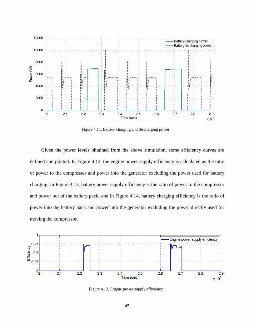
Given the power levels obtained from the above simulation, some efficiency curves are
defined and plotted. In Figure 4.12, the engine power supply efficiency is calculated as the ratio
of power to the compressor and power into the generator excluding the power used for battery
charging. In Figure 4.13, battery power supply efficiency is the ratio of power to the compressor
and power out of the battery pack, and in Figure 4.14, battery charging efficiency is the ratio of
power into the battery pack and power into the generator excluding the power directly used for
moving the compressor.
Figure 4.11. Battery charging and discharging power
Figure 4.12. Engine power supply efficiency

46
Besides the power and efficiency performance, a few other details may be of interest to
engineers. The generator and motor power factors are plotted in Figure 4.15. A 6-kWh battery
pack is selected for this simulation. Its stored energy is used to drive the compressor when the
truck engine is off. The battery gets charged when external power sources are available. In this
study, the source is the generator. However, the source may also be a “shore” grid power. The
battery’s SOC and terminal voltage are simulated in Figure 4.16 and Figure 4.17, respectively.
Figure 4.13. Battery power supply efficiency
Figure 4.14. Battery charging efficiency

47
Figure 4.15. IM and PMSM power factor
Figure 4.16. Battery SOC change
Figure 4.17. Terminal voltage of the battery pack

48
With all the above power system and thermal system components integrated properly, a
desired temperature profile is achieved as shown in Figure 4.18. The compressor is able to
supply the right amount of cooling air to maintain product temperature within the desired -25 °C
to -30 °C range.
Figure 4.18. Temperature change in the container

49
4.2 Detailed Model Simulation
A detailed dynamic power system model with exactly the same parameters is constructed in
Simulink/SimPowerSystems. The detailed model includes stepping waveforms from the
semiconductor devices at each switching action, taking consideration of snubber circuits. It
models the electric machines (PMSM, IM) as differential equations that produce transient
waveforms. Filters are also included between components, and harmonics analysis can be
performed. However, the model’s simulation sampling time is a maximum 5 µs, and it produces
only two simulation seconds in three minutes. Figure 4.19 shows a dynamic response of the rotor
speed, stator current, and electromagnetic torque of the IM during the compressor start. The
system is chosen to start from 5400 s. Note that it takes about 0.5 s for the rotor to ramp up to the
desired speed, 1720 RPM. After another half second when a higher 1780 RPM speed is desired,
further transient response is observed. Figure 4.20 shows that the dc bus voltage is feedback
controlled to be 700 V all the time, and the inverter PWM modulation index is ramped up
gradually to the desired value. In addition, details of the high-frequency switching IM stator
voltage can be observed.

50
The detailed model serves as a validation check for the average model. Although it is not
feasible for the detailed model to run as long as a few simulation hours like the average model, it
is still possible to simulate the system conditions for a few selected points. Figure 4.21 plots 10
efficiency values on the engine power supply efficiency curve (Figure 4.12), and Table 4.1 lists
Figure 4.19. Transient response of IM
Figure 4.20. Transient response at the inverter

51
the detailed data for these 10 points. Notice that the two efficiency curves are within 5% of each
other. Generally, the detailed model efficiency is somewhat lower. This is expected because the
detailed model includes complete losses from harmonics, snubber circuits, precise switching
actions, and refined machine subsystems. However, for this system, the energy flow and
efficiency trend over a long time interval is wanted; hence the loss of the details is not a major
concern.
Time (sec) Generator
RPM Motor RPM
Torque
(Nm)
Input Power
(W)
Output Power
(W) Efficiency
22240 2909 1786 15.31 5132 3099 0.603
22270 4056 1782 19.56 5818 3891 0.668
22300 4233 1779 22.76 6604 4479 0.678
22330 4227 1778 24.11 6936 4797 0.691
22360 3899 1777 24.62 6890 4818 0.699
22390 3689 1777 24.78 6918 4849 0.700
22420 3571 1777 24.82 6932 4858 0.700
22450 4188 1777 24.83 7048 4860 0.689
22480 3863 1777 24.82 6934 4855 0.700
22510 3347 1777 24.8 6970 4850 0.695
Figure 4.21. Simulated efficiency comparison for average and detailed models
Table 4.1. Simulated power and efficiency data for the detailed model

52
5 EXPERIMENTAL VALIDATION
The system outlined by Figure 2.3 with the desired component specifications is difficult to
realize physically at the moment. However, it is possible and reasonable to break the system into
three parts and test them individually. The first part, the front end, consists of the generator and
the ac-dc rectifier. The battery pack is the second part. The last is the variable frequency ac
motor drive, including the dc-ac inverter and the motor.

53
5.1 Front End Testing
The front end test was conducted by a division of Ingersoll Rand, associated with Thermo King,
in Prague, Czech Republic [28]. This 17.3 kVA machine was exactly the same as the one
modeled in Simulink. It was used previously as the generator for an electric air conditioning unit
in a city bus. Different loads were applied for each of various speed/RPM settings, and the
corresponding powers and efficiencies were obtained through direct measurement, as shown in
Figure 5.1. In the same test, Figure 5.2 shows the power losses and efficiencies versus speed for
each load (torque) applied. The simulated power losses and efficiencies are plotted in dashed
lines; and solid lines show the actual data. It can be observed that the simulation power loss
prediction is within 6% deviation from the actual data over most of the operating range. The
simulated and measured efficiencies are within 1% of each other. Figure 5.3 is a comprehensive
efficiency map for this PMSM. The many distributed dots on the figure are actual experimental
data points.
Figure 5.1. PMSM efficiency versus power at different speeds [29]

54
Figure 5.2. PMSM power loss and efficiency versus speed at different loads [29]
Figure 5.3. Efficiency map for PMSM [29]

55
The ac-dc rectifier was also tested in Prague [28]. A 600 V/40 A PWM rectifier was used.
It was connected to the generator output, and power data were obtained for different generator
RPMs and output powers, as shown in Figure 5.4. Overall the percent efficiency was high, in the
upper 90 percentile. This was expected for a PWM rectifier with these ratings. This matched the
model simulation.
90
91
92
93
94
95
96
97
98
99
100
0 2 4 6 8 10 12 14 16
Effi
cie
ncy
(%
)
P_dc (kW)
1500 RPM
2070 RPM
2500 RPM
3000 RPM
3500 RPM
4000 RPM
4500 RPM
5000 RPM
Figure 5.4. Rectifier efficiency versus power for different PMSM speeds [29]

56
5.2 Battery Testing
The second part is the battery test. To validate the improved modeling approach, test data for the
R and C constants and open circuit voltage in Figure 3.10 were obtained and plotted against the
model simulation. The test data are available from the appendix in [25]. Figures 5.5 to 5.10 show
the curve-fitted and measured data for discharging R second, C second, R minute, C minute, R
hour, and C hour constants, as functions of SOC, as described in Section 3.5. Figure 5.11 shows
the simulated and measured battery cell open circuit terminal voltages as functions of SOC. All
the fitted/simulated curves demonstrate close relationships with the measured data without
showing severe ups and downs that can cause simulation’s instability.
Figure 5.5. Measured R_sec constant compared to fitted curve
Figure 5.6. Measured C_sec constant compared to fitted curve

57
Figure 5.7. Measured R_min constant compared to fitted curve
Figure 5.8. Measured C_min constant compared to fitted curve
Figure 5.9. Measured R_hour constant compared to fitted curve
Figure 5.10. Measured C_hour constant compared to fitted curve

58
Figure 5.11. Measured battery terminal voltage compared to simulated data
59
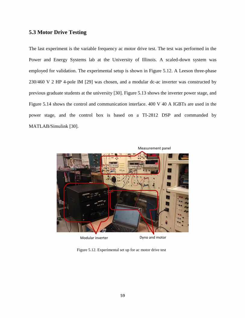
5.3 Motor Drive Testing
The last experiment is the variable frequency ac motor drive test. The test was performed in the
Power and Energy Systems lab at the University of Illinois. A scaled-down system was
employed for validation. The experimental setup is shown in Figure 5.12. A Leeson three-phase
230/460 V 2 HP 4-pole IM [29] was chosen, and a modular dc-ac inverter was constructed by
previous graduate students at the university [30]. Figure 5.13 shows the inverter power stage, and
Figure 5.14 shows the control and communication interface. 400 V 40 A IGBTs are used in the
power stage, and the control box is based on a TI-2812 DSP and commanded by
MATLAB/Simulink [30].
Measurement panel
Dyno and motor
Modular inverter
Figure 5.12. Experimental set up for ac motor drive test

60
Figure 5.15 is a simulated motor drive characteristic plot for the specified three-phase
230/460 V 12 HP 4-pole IM. It shows the IM torque-speed curve at 60 Hz and also along with its
efficiency, power, and current curves. Experiments to verify these curves will be run at various
frequencies on the modular inverter and the 2 HP IM. The inverter was controlled by the V/f
Figure 5.13. Power stage for the modular inverter
Figure 5.14 Control board for the modular inverter

61
technique to vary the frequencies and voltages. Figure 5.16 shows sampled points giving the
torque-speed curve at 50, 60, and 70 Hz, respectively. Similarly the efficiency and power curves
were obtained in Figures 5.17 and 5.18, respectively. Although the measured data matched the
simulated curves (scaled down), it is important to note that the nominal efficiency is 84.0% for
the 2 HP IM [29], whereas it is 89.2% for the 12 HP IM, the machine used for simulation.
Figure 5.15. Simulated machine parameters for the 12 HP IM
Figure 5.16. Measured IM torque speed curve at different frequencies

62
The dynamometer acted as the load and was programmed to impose the torque profile
from Figure 5.19 to the IM. The torque profile was selected from Figure 4.7 and scaled to 1/6 of
the original to fit the 2 HP machine. Similarly, a speed control command, as shown in Figure
5.20, was realized by the inverter through V/f control. The running time was 720 seconds.
During this time, output and input power were measured across the entire motor drive, and an
efficiency curve was plotted in Figure 5.21. The measured efficiency was on average about 5%
lower than the simulated efficiency. This was expected because the IM used for this experiment
has an efficiency value about 5% lower. Nevertheless, the measured efficiency trend closely
matched the expected efficiency. This demonstrates that the average model is accurate.
Figure 5.17. Measured IM efficiency versus speed at different frequencies
Figure 5.18. Measured IM power versus speed at different frequencies

63
Figure 5.19. Desired torque demand for the motor drive
Figure 5.20. Desired speed command for the ac motor drive
Figure 5.21. Measured efficiency compared to simulated efficiency for the motor drive

64
6 DISCUSSION
The detailed model simulation and experimental validation have demonstrated the accuracy of
the average model, which will be used to calculate energy and cost-effectiveness for the hybrid
power system. These results will be compared to the conventional power system.
Assumptions on truck operating conditions, drive cycles, and battery pack selections are
required in order to calculate energy consumption for different power system configurations. The
simulated scenario in Chapter 4 is used and extended to 0 s to 36,000 s to represent a whole day,
as described in Table 3.1. Simulation results are similar to those in Figures 4.2 to 4.18. A battery
pack is pre-charged from the grid before deliveries, and it is charged by the generator during the
deliveries. A 6 kWh battery pack is chosen such that it just gets depleted by the end of the day.
The battery is then recharged from the grid. Under these assumptions, the MRU energy used
throughout the day is drawn from the generator in addition to a one-time fully charged battery
pack.
The generator input energy, computed by integrating the generator input power over time,
is found to be 95.15 MJ. The National Petroleum Council estimates that the diesel engine of this
medium-duty class 6 truck has a 40% efficiency [8]. Therefore, the total daily diesel energy
required is approximately 237.87 MJ. Note that the pre-charged battery pack contains 21.6 MJ.
Assuming it is charged with a 90% efficient charger, 24.0 MJ is consumed from the grid. On the
other hand, the conventional power system requires 83.19 MJ, calculated by integrating the
compressor power. If the compressor is directly coupled to a diesel engine, 332.76 MJ diesel fuel
is required, assuming that this engine is light-duty with 25% efficiency [8]. Table 6.1
summarizes energy calculations. The table also includes the total cost per day to supply energy in

65
hybrid and conventional power systems, assuming 135.6 MJ/gal in the diesel fuel [8] at $4.00/gal
and $0.10/kWh for electricity [31].
Hybrid Conventional
Diesel fuel (gal) 1.75 2.45
Electricity (kWh) 6.67 0
Total energy (MJ) 261.87 332.76
Total cost ($) 7.67 9.80
It can be observed that the hybrid power system saves approximately 71 MJ (0.53 gal of
diesel or 19.5 kWh of electricity) and $2.13 per day compared to the conventional system. Note
that this is based on the assumption that the truck engine is 40% efficient (hybrid case) and the
compressor coupled engine is 25% efficient (conventional case). These efficiency numbers may
vary depending on the actual engines chosen. In particular, if the compressor-coupled engine is
above 31.8% efficient, the hybrid power system is no longer advantageous. The above analysis
shows that the hybrid power system for MRUs is only somewhat efficient. As mentioned in
Chapter 1, this hybrid system lacks the possibility of regenerative braking, as used in HEV
applications. Nevertheless, the hybrid MRUs at least eliminate pollution while the truck idles.
This complies with various regulations and is environmentally friendly.
An ac grid plug-in option inserted between the generator and the rectifier (Figure 2.3)
may increase energy savings. This option is enabled when the truck is stopped and a “shore” grid
power is available. The battery pack size could be reduced because the compressor is powered
directly from the grid. Hence less energy is required to charge the battery from the inefficient
Table 6.1. Energy and cost comparison between hybrid and conventional systems
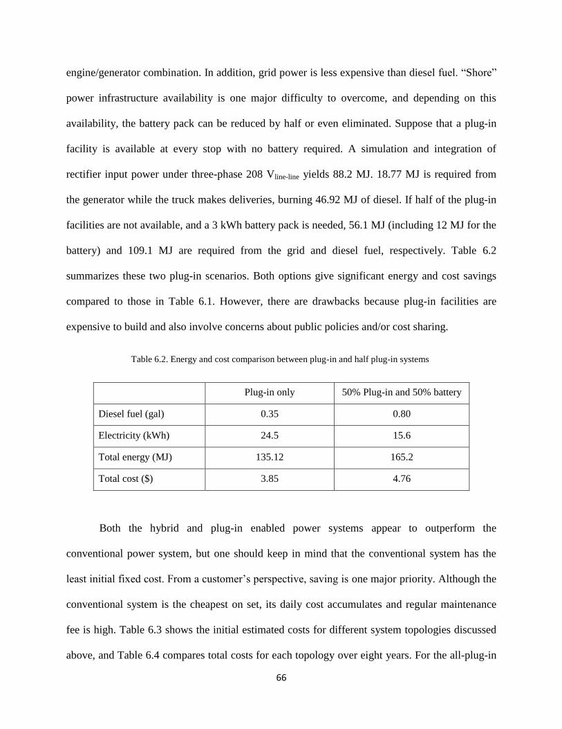
66
engine/generator combination. In addition, grid power is less expensive than diesel fuel. “Shore”
power infrastructure availability is one major difficulty to overcome, and depending on this
availability, the battery pack can be reduced by half or even eliminated. Suppose that a plug-in
facility is available at every stop with no battery required. A simulation and integration of
rectifier input power under three-phase 208 Vline-line yields 88.2 MJ. 18.77 MJ is required from
the generator while the truck makes deliveries, burning 46.92 MJ of diesel. If half of the plug-in
facilities are not available, and a 3 kWh battery pack is needed, 56.1 MJ (including 12 MJ for the
battery) and 109.1 MJ are required from the grid and diesel fuel, respectively. Table 6.2
summarizes these two plug-in scenarios. Both options give significant energy and cost savings
compared to those in Table 6.1. However, there are drawbacks because plug-in facilities are
expensive to build and also involve concerns about public policies and/or cost sharing.
Plug-in only 50% Plug-in and 50% battery
Diesel fuel (gal) 0.35 0.80
Electricity (kWh) 24.5 15.6
Total energy (MJ) 135.12 165.2
Total cost ($) 3.85 4.76
Both the hybrid and plug-in enabled power systems appear to outperform the
conventional power system, but one should keep in mind that the conventional system has the
least initial fixed cost. From a customer’s perspective, saving is one major priority. Although the
conventional system is the cheapest on set, its daily cost accumulates and regular maintenance
fee is high. Table 6.3 shows the initial estimated costs for different system topologies discussed
above, and Table 6.4 compares total costs for each topology over eight years. For the all-plug-in
Table 6.2. Energy and cost comparison between plug-in and half plug-in systems
systems

67
option, suppose ten customers share costs to build ten charging stations, each customer is
responsible for one station. For the hybrid/plug-in option, only five stations are required, and
each customer incurs half the construction cost. The truck is expected to operate 6 days a week,
or 312 days per year. Every year the diesel engine for the conventional system requires regular
oil/filter and air filter changes at an estimated cost of $500, including labor.
Conventional Hybrid Plug-in only Hybrid/plug-in
Light-duty engine $800 $0 $0 $0
Battery pack and converter $0 $2650 $0 $1500
PMSM, IM, power
electronic converters, wiring $0 $2950 $2950 $2950
Charger and charging station $0 $0 $4200 $2100
Total $800 $5600 $7150 $6550
Conventional Hybrid Plug-in only Hybrid/plug-in
Beginning $800 $5600 $7150 $6550
In one year $4358 $7993 $8351 $8035
In two years $7916 $10386 $9552 $9520
In three years $11474 $12779 $10753 $11005
In four years $15031 $15172 $11954 $12490
In five years $18590 $17565 $13155 $13975
In six years $22148 $19958 $14356 $15460
In seven years $25706 $22351 $15557 $16945
In eight years $29264 $24744 $16758 $18430
Table 6.3. Initial costs for different power system configurations
Table 6.4. Total costs of the first eight years for different power system configurations

68
Figure 6.1 plots the data in Table 6.4. The figure shows that after three years the options
with plug-in outperform the conventional system, and after four years, the hybrid option also
becomes advantageous. Note that a large portion of plug-in fixed costs comes from chargers or
charging stations. It may take less time for break-even if such cost is not directly out of a
customer’s pocket or if a “charging station” is just an electric outlet. The purely plug-in system is
somewhat but not much cheaper than the hybrid/plug-in option in the long run. However, the
hybrid/plug-in configuration is more adaptive and can function if a charging station is not
available at every stop.
Figure 6.1. Comparison of total costs over eight years for different topologies
The analysis above is based on the operating conditions described in Chapter 4. Other
operating conditions may likely yield different energy and cost savings results. For example, if
the truck makes mostly inter-city deliveries, the plug-in options are less attractive because there
are few stops. In this case, the hybrid power system seems the best option to comply with
environmental regulations. With other scenarios considered, a comprehensive energy and cost
savings analysis is required for the future in order to target different customers’ MRU
applications.

69
7 CONCLUSION AND FUTURE WORK
A hybrid power system for mobile refrigeration applications has been designed, modeled, and
tested. The proposed average model, interfaced with the thermal system model, has been
validated by comprehensive simulation and experimental work. The average model with
improved battery formulation enhances accuracy and robustness for the battery subsystem
simulation. In addition to fast simulation, the model is flexible and can run at desired times,
power levels, and drive cycles. A user-friendly model block library, including various machine
types (IM, PMSM, etc.), battery types (Li-ion, lead-acid, etc.), along with different power
converters, has been released. These model blocks can be substituted in the system on a modular
basis for various potential prototypes. The average model has been applied as part of a complete
thermal-electric system simulation and serves as a basis for future energy storage selection and
hybrid system optimization studies.
There are a few comments about the average model’s limitations and considerations. 1)
The model runs fast by trading off fidelity. The model is not intended for use in detailed
hardware design, and it is not helpful for observing system behavior in a short time interval
especially during traction system’s instantaneous acceleration or deceleration. 2) Various drive
cycles and loading profiles are appropriate for a most thorough system analysis. The scenario
described in this thesis is keeping produce frozen inside the truck container on a hot summer day
for a local delivery truck. Another scenario of a truck’s non-stop running on a highway for a few
hours will have a different output result. It may also be required to maintain a certain produce
temperature above 0 °C on a -20 °C winter day. In this case, the MRU must supply warm air, and
depending on the heating unit, the power system may or may not be modified. 3) The hybrid
model presented is based on a parallel-hybrid topology. On the other hand, a series-hybrid or
70
other topology may be equivalently functional. One alternative directly couples the PMSM with
the IM. The idea is feasible because the PMSM itself acts like a volts-per-hertz control due to the
linear relationships between V, f and rotor speed. However, further study may be required, as the
PMSM has a wide range of outputs and there are limitations. 4) The system was validated
through three parts in Chapter 5. A complete test at full scale needs to be performed to
completely demonstrate the model accuracy.
The electrification of an MRU is a recent topic in industry and has enormous
opportunities for research and development. The average model presented in this thesis may lead
to multiple directions of improvement. 1) Advanced existing or novel control techniques can be
applied to the motor drive for highly efficient and precise internal loading requirement. This may
be particularly beneficial for highly temperature-sensitive products such as medications. 2) A
multilevel converter based motor drive is worth investigating for improving efficiency and
reducing motor stress, especially under high power requirements. The system can be equipped
with different battery types such as nickel-metal hydride or alternative energy storage devices
such as fuel cells. These energy devices can be studied for performance, cost-effectiveness, and
efficiency. 3) A grid plug-in is definitely an option, as discussed in Chapter 6. The typical power
requirement is less than 5 kW, and a three-phase shore power is readily available. A
comprehensive energy and cost analysis for different system configurations and truck operating
situations can be further pursued. 4) We want to know what is the optimal operation strategy
considering the truck engine, battery, and plug-in on and off status, to have the highest efficiency
while enjoying a low cost. 5) Try to explore another modeling strategy, such as the piece-wise
linear method suggested by [19], which is capable of reaching the simulation speed goal but also
providing more details.

71
REFERENCES
[1] CARB, “Airbourne toxic control measure for in-use diesel fueled transportation refrigeration
units (TRU) and TRU generation units, and facilities where TRUs operate,” California Air
Resources Board, 2003.
[2] R. R. Hammond, “Engine performance analysis of a diesel auxiliary power unit used to
eliminate heavy duty truck idling,” M.S. thesis, University of California, Davis, 2001.
[3] C. V. Kulkarni, “Modeling and the performance analysis of transportation refrigeration units
with alternate power systems,” Ph.D. dissertation, Mechanical and Aeronautical Engineering,
Univ. of California, Davis, 2007.
[4] EPRI, “Transportation refrigeration equipment: cost-effective emissions reduction,” EPRI
Rep. 1008774, 2004.
[5] D. Karner and J. Francfort, “US Department of Energy hybrid electric vehicle battery and
fuel economy testing,” Journal of Power Sources, vol. 158, no. 2, pp. 1173-1177, Aug. 2006.
[6] B. Mohs, et al., “Truck hybridization architecture and control study – Thermo King and
Ingersoll Rand,” unpublished, 2011.
[7] C. C. Chan, “The state of the art of electric, hybrid, and fuel cell vehicles,” Proceedings of
the IEEE, vol. 95, no. 4, pp. 704-718, 2007.
[8] National Petroleum Council, “Heavy-duty engines & vehicles analysis – advancing
technology for America’s transportation future,” National Petroleum Council report, 2012.
[9] T. Chun et al., “Simulator for monitoring the operations of range extender electric vehicles,”
Journal of Power Electronics, vol. 11, no. 4, pp. 424-429, 2011.
[10] T. W. Ching, “An investigation on electrical performance of variable-frequency drives for
air-conditioning applications,” IEEE Electrical Power & Energy Conference, 2008, pp. 1-7.
[11] S. Shao et al., “Performance representation of variable speed compressor for inverter air
conditioners based on experimental data,” International Journal of Refrigeration, vol. 27,
pp. 805-815, 2004.
[12] K. L. Butler et al., “A Matlab-based modeling and simulation package for electric and
hybrid electric vehicle design,” IEEE Transactions on Vehicular Technology, vol. 48, no. 6,
pp. 1770-1778, Nov. 1999.
[13] C. Lin, “Modeling and control strategy development for hybrid vehicles,” Ph.D.
dissertation, University of Michigan, Ann Arbor, 2004.
[14] M. Amrhein and P. T. Krein, “Dynamic simulation for analysis of hybrid electric vehicle
system and subsystem interactions, including power electronics,” IEEE Transactions on
Vehicular Technology, vol. 54, no. 3, pp. 825-836, May 2005.

72
[15] B. Y. Liaw et al., “Modeling of lithium-ion cells – a simple equivalent-circuit model
approach,” Solid State Ionics, vol. 175, pp. 835-839, 2004.
[16] L. Gao, S. Liu, and R. A. Dougal, “Dynamic lithium-ion battery model for system
simulation,” IEEE Transactions on Components and Packaging Technology, vol. 25, no.
3, pp. 495-505, September 2002.
[17] C. Unterrieder et al., “Comparative study and improvement of battery open circuit voltage
estimation methods,” IEEE International Midwest Symposium on Circuits and Systems, pp.
1076-1079, 2012.
[18] H. He et al., “Online model-based estimation of state-of-charge and open-circuit voltage of
lithium-ion batteries in electric vehicles,” Energy, vol. 30, no. 1, pp. 310-318, March 2012.
[19] J. H. Allmeling and W. P. Hammer, “PLECS - piece-wise linear electrical circuit simulation
for Simulink,” IEEE International Conference on Power Electronics and Drive Systems,
1999, pp. 355–360.
[20] A. Abramovitz, “An approach to average modeling and simulation of switch-mode
systems,” IEEE Transactions on Education, vol. 54, no. 3, pp. 509-517, 2011.
[21] A. E. Fitzgerald, C. Kingsley, and S. D. Umans, Electric Machinery, 6th
ed. New York:
McGraw Hill, 2003, pp. 306-348.
[22] P. C. Krause, O. Wasynczuk, and S. D. Sudhoff, Analysis of Electric Machinery and Drive
Systems, 2nd
ed. Edison, NJ: Wiley-IEEE Press, 2002, pp. 525-556.
[23] P. T. Krein, Elements of Power Electronics, 1st ed. New York: Oxford University Press,
1998, pp. 451-530.
[24] R. C. Kroeze and P. T. Krein, “Electrical battery model for use in dynamic electric vehicle
simulations,” IEEE Power Electronics Specialists Conf., Rhodes, Greece, 2008, pp. 1336-
1342.
[25] R. C. Kroeze, “Electrical battery model for use in dynamic electric vehicle simulations,”
M.S. thesis, Electrical and Computer Engineering, Univ. of Illinois, Urbana, IL, 2008.
[26] US EPA, “Drive cycle development,” EPA Smartway Truck Emissions Test Protocol
Workshop, US Environmental Protection Agency, 2008.
[27] R. A. Jackey, “A simple, effective lead-acid battery modeling process for electrical system
component selection,” The Mathworks Inc., Novi, MI, Rep. 2007-01-0778, 2007.
[28] P. Kadanik et al., “Transport hybridization study sponsor update – Thermo King and
Ingersoll Rand,” unpublished, 2012.
[29] Leeson 230/460 2 HP Induction Machine, Datasheet.
[30] J. Kimball et al., “Modular inverter for advanced control applications,” Grainger Center for
Electric Machinery and Electromechanics, Urbana, IL, CEME-TR-2006-01, 2006.

73
[31] BLS, “Average energy prices in the Chicago area,” Bureau of Labor Statistics, Midwest
Information Office, 13-233-CHI, 2013.

74
APPENDIX A SIMULINK MODELS
A.1 High-Level Integrated Thermo-Electric Model
Figure A.1 High-level integrated thermo-electric model in MATLAB/Simulink
A.2 Average Model for Hybrid Power Systems
Figure A.2 High-level hybrid power systems average model in MATLAB/Simulink
Controller
Thermal System
Power System
Truck Container
Drive Cycle

75
A.3 Detailed Model for Hybrid Power Systems
Figure A.3 High-level hybrid power systems detailed model in MATLAB/Simulink

76
APPENDIX B MATLAB PROGRAMS
B.1 IM Parameters Calculation MATLAB Code
close all, clear all, clc
% Two rated voltages (this is line-line RMS) V_rated = [460; 400]; % first entry is bigger than the second entry
% Corresponding frequencies in Hz Freq_rated = [60; 50];
% Corresponding locked currents I_locked = [123; 116];
% Locked rotor torque at first frequency T_locked = 126;
% Number of poles pole = 4;
% Power factor at first frequency PF = 0.88;
% Efficiency at first frequency Eff = 0.892;
% Rated horse power at first frequency HP = 12;
% Rated RPM at first frequency RatedRPM = 1750;
% End of inputs % --------------------------------------------------------------
Z_rated = (V_rated/sqrt(3))./I_locked; % per phase % Z_rated = (R1+R2) + j*2*pi*freq*(L1+L2) = R + j*2*pi*freq*L
L = sqrt(((Z_rated(1))^2-(Z_rated(2))^2)/((2*pi*Freq_rated(1))^2-
(2*pi*Freq_rated(2))^2)); % R^2 + (2*pi*f*L)^2 = Z^2, freq is different R = sqrt((Z_rated(1))^2 - (2*pi*Freq_rated(1)*L)^2);
L2 = 0.5*L L1 = 0.5*L % Usually L1=L2=0.5L
R2 = T_locked*(2*pi*Freq_rated(1)/(pole/2))/3/(I_locked(1))^2 % T = 3*I^2*R2 / (2*pi*f/pole_pairs) R1 = R - R2

77
I1_mag = HP*746/Eff/PF/3/(V_rated(1)/sqrt(3)); % 1 HP = 746 W Angle1 = -1*acos(PF); % Lagging power factor for IM I1 = I1_mag*exp(j*Angle1); % Phasor format
V_shunt = V_rated(1)/sqrt(3) - I1*(R1+j*2*pi*Freq_rated(1)*L1); % V_shunt = Vin - I1*Z1, Vin as reference with angle 0
SyncRPM = 120*Freq_rated(1)/pole; % SyncRPM = 120*f/pole slip = 1 - RatedRPM/SyncRPM;
I2 = V_shunt/(R2/slip+j*2*pi*Freq_rated(1)*L2); % I2 = V_shunt/Z2 I_shunt = I1-I2;
Y_shunt = I_shunt/V_shunt; % Admittance of shunt branch % Y_shunt = 1/Rc + 1/(j*2*pi*f*Lm)
Lm = 1/abs(imag(Y_shunt))/(2*pi*Freq_rated(1)) Rc = 1/abs(real(Y_shunt)) % Match the corresponding component of Y_shunt
B.2 PMSM Parameters Calculation MATLAB Code
clear all, close all, clc
% RPM column: RPM = [1500; 1875; 2250; 3000; 4500; 5000];
% No load voltage at 20C (this is line-line RMS) Volt = [195; 244; 293; 390; 585; 650];
% Frequency column Freq = [100; 125; 150; 200; 300; 334];
% End of inputs % ------------------------------------------------------------
Frequency_Constant = mean(Freq./RPM)*1000 % linear relations Voltage_Constant = mean(Volt./RPM)*1000/sqrt(3) % linear relations and
convert to line-neutral RMS


![[] Hybrid Self-Organizing Modeling org](https://img.pdfslide.us/doc/110x75/543c51adafaf9fe8338b4707/-hybrid-self-organizing-modeling-org.jpg)