Modeling river plume dynamics with the HYbrid Coordinate ...Ocean... · Modeling river plume dynamics with the HYbrid Coordinate Ocean Model ... Numerical modeling ... We employ the

Ocean Modelling 33 (2010) 101–117

Contents lists available at ScienceDirect

Ocean Modelling

journal homepage: www.elsevier .com/locate /ocemod

Modeling river plume dynamics with the HYbrid Coordinate Ocean Model

Rafael V. Schiller *, Vassiliki H. KourafalouUniversity of Miami, Rosenstiel School of Marine and Atmospheric Science, RSMAS/MPO, 4600 Rickenbacker Cswy, Miami, FL, USA

a r t i c l e i n f o

Article history:Received 9 June 2008Received in revised form 7 December 2009Accepted 13 December 2009Available online 21 December 2009

Keywords:River plumesNumerical modelingCoastal processesHYCOM

1463-5003/$ - see front matter � 2009 Elsevier Ltd. Adoi:10.1016/j.ocemod.2009.12.005

* Corresponding author. Tel.: +1 305 421 4654; faxE-mail addresses: [email protected] (R.V

mas.miami.edu (V.H. Kourafalou).

a b s t r a c t

The dynamics of large-scale river plumes are investigated in idealized numerical experiments using theHYbrid Coordinate Ocean Model (HYCOM). The focus of this study is to address how the development andstructure of a buoyant plume are affected by the outflow properties, as impacted by processes within theestuary and at the point of discharge to the coastal basin. Changes in the outflow properties involved ver-tical and horizontal redistribution of the river inflow and enhanced vertical mixing inside an idealizedestuary. The development of the buoyant plume was evaluated in a rectangular, f-plane basin with flatand sloping bottom conditions and in the absence of other external forcing. The general behavior of amid-latitude river plume was reproduced, with the development of a surface anticyclonic bulge off theestuary mouth and a surface along-shore coastal current which flows in the direction of Kelvin wavepropagation (‘‘downstream”); the momentum balance was predominantly geostrophic. Conditionswithin the estuary and the outflow properties at the river mouth (where observed profiles may be avail-able) greatly impacted the fate of riverine waters. In flat bottom conditions, larger mixing at the freshwa-ter source enhanced the estuarine gravitational circulation, promoting larger upward entrainment andstronger outflow velocities. Although the overall geostrophic balance was maintained, estuarine mixingled to an asymmetry of the currents reaching the river mouth and to a sharp anticyclonic veering withinthe estuary, resulting in reduced upstream flow and enhanced downstream coastal current. These pat-terns were altered when the plumes evolved in the presence of a bottom slope. The anticyclonic veeringof the buoyant outflow was suppressed, the offshore intrusion decreased and the recirculating bulge wasdisplaced upstream. The sloping bottom impacts were accompanied by enhanced transport and increaseddownstream extent of the coastal current in most cases. No major changes in the general properties andespecially the vertical structure of the plumes were observed when the vertical coordinates were changedfrom cartesian–isopycnal, to sigma or to sigma–isopycnal. The findings offer a benchmark for coastalstudies with HYCOM, where plume dynamics should be examined in tandem with additional circulationforcing mechanisms, resulting in transitions of the vertical coordinate system that are dictated by theprevailing dynamics.

� 2009 Elsevier Ltd. All rights reserved.

1. Introduction

The dynamics of large-scale river outflows (affected by theearth’s rotation) have been widely investigated in the literature.It is acknowledged that in the absence of external forcing (suchas winds, tides, and ambient currents) and if a river buoyant plumeis large enough to be affected by the Coriolis force, riverine waterswill turn anticyclonically when they reach the shelf, and moveaway from their land source as an along-shore buoyancy drivencoastal current, in the direction of Kelvin wave propagation (here-after referred to as ‘‘downstream direction”). Observations of largeriver plumes on open shelves such as along the US east and westcoasts include: the Delaware (Münchow and Garvine, 1993a,b)

ll rights reserved.

: +1 305 421 4696.. Schiller), vkourafalou@rs-

and the Chesapeake (Boicourt, 1973; Marmorino and Trump,2000) Bays, the Columbia (Hickey et al., 1998, 2005; Horner-De-vine, 2009), the Hudson (Chant et al., 2008) and the Niagara (Masseand Murthy, 1992; Horner-Devine et al., 2008) Rivers, and the lowsalinity coastal band in the South Atlantic Bight (Blanton et al.,1994). Satellite and field studies have also shown evidence of abulge-like region in the vicinity of the river inflow, where plumewaters recirculate before feeding the coastal current (Masse andMurthy, 1992; Hickey et al., 1998; Chant et al., 2008; Horner-De-vine et al., 2008; Horner-Devine, 2009). Similar behavior has alsobeen observed in laboratory studies (Stern et al., 1982; Griffithsand Hopfinger, 1983; Whitehead and Chapman, 1986; Avicolaand Huq, 2003a,b; Horner-Devine et al., 2006).

In addition to observations, numerical and analytical modelshave been used to understand and clarify the dynamics of coastalbuoyant plumes. Many studies have been conducted in idealizedscenarios. Rectangular basins were employed with simplified

http://dx.doi.org/10.1016/j.ocemod.2009.12.005

mailto:[email protected]



http://www.sciencedirect.com/science/journal/14635003

http://www.elsevier.com/locate/ocemod

102 R.V. Schiller, V.H. Kourafalou / Ocean Modelling 33 (2010) 101–117

bottom topography, with buoyancy forcing only or with additionalsimple external forcing, such as constant and unidirectional winds,along-shore ambient current and single component tides. Such ide-alized studies revealed many features of river plume dynamicsgenerally hard to extract from observations, where complex circu-lation forcing mechanisms impact the plume behavior. Early stud-ies recognized the importance of non-linearity, rotation andfriction in the development of the frontal structure of large buoy-ant discharges (Kao et al., 1977; Kao, 1981; Ikeda, 1984; Garvine,1987). Pioneering numerical modeling studies demonstrated theimpact of vertical mixing, bottom drag and sloping bottom onthe spin-up, maintenance and dissipation of river-forced plumes(Chao and Boicourt, 1986; Chao, 1988a,b) as well as the coastalcurrent variability associated with barotropic and baroclinic insta-bilites (Oey and Mellor, 1993). The variability of the bulge and thecoastal current from a river-forced plume was also demonstratedby Kourafalou et al. (1996), who ellucidated the effects of buoy-ancy-induced stratification versus available mixing in determiningthe expansion of the bulge and the coastal current meandering.

The importance of the river mouth conditions to the variabilityof the bulge and coastal current transport has been reported byseveral studies. Yankovsky and Chapman (1997) developed a the-ory which relates properties of the estuarine discharge and cross-shore bottom slope to the bulge and coastal current structure. Gar-vine (1999) verified that the estuarine volume transport, scaled bythe associated outflow geostrophic transport, controlled the great-est variance of the downshelf and across-shelf plume penetration.Fong and Geyer (2002) demonstrated that river mouth conditionsaffect the amount of freshwater transported by the coastal currentrelative to the bulge, which can accumulate low salinity waters,become unsteady and grow in time. They observed that when riveroutflows with larger Rossby number were simulated, more plumewater recirculated within the bulge and that decreased the coastalcurrent freshwater transport. In a series of laboratory experiments,Avicola and Huq (2003a,b) demonstrated how the ‘‘outflow angle”(angle between the outflow and the coastal wall) and the ‘‘impactangle” (angle at which the buoyant flow reattaches to the coast) af-fect the formation of the recirculating bulge. They suggested thatthe two angles are related (the outflow angle determines the im-pact angle) and concluded that a coastal current formed at obliqueimpact angles, and the bulge recirculation increased as the impactangle approached 90�. Finally, Yankovsky (2000) and Garvine(2001) demonstrated that the implementation of the river bound-ary conditions may affect the near-field bulge circulation, morespecifically the development of the plume upstream intrusion.Kourafalou et al. (1996) showed that the upstream intrusion wasdue to a non-geostrophic balance between the along-shore acceler-ation and the along-shore pressure gradient (due to low salinitywaters near the river mouth and denser ambient waters up thecoast). Yankovsky (2000) suggested that the upstream intrusionis enhanced by over simplified river boundary conditions that lacka baroclinic adjustment of the discharge (i.e., fixed uniform riverinflow along the coastal wall). The blocking of the lower layer land-ward flow at the mouth promotes a strong cyclonic vorticity dis-turbance with corresponding upstream turning of the buoyantflow at the source, which enhances the upstream spreading ofthe plume. Yankovsky (2000) and Garvine (2001) concluded thatthe use of an inlet flow field that better mimics that observed atthe mouth of estuaries (upper seaward buoyant flow on top of alower landward undercurrent) reduces that impact.

In the study presented herein, a ocean general circulation modelis employed in an idealized estuary-coastal basin system to exam-ine the development and evolution of a river plume under buoy-ancy forcing only and to investigate the plume variabilityassociated with changes in the conditions at the river mouth. Thesechanges are shown to be the results of lateral and vertical spread-

ing of the river inflow and variable mixing inside the estuary. Theseeffects are expected to impact the estuarine circulation and thebuoyant outflow, ultimately promoting changes in the recirculat-ing bulge and the coastal current properties. Previous numericalmodeling studies (Chao and Boicourt, 1986; Chao, 1988a; MacC-ready et al., 2009) have demonstrated the importance of the estu-arine circulation to the development of the river plume. The focusof the study presented herein is to understand how the propertiesof the buoyant flow at the estuary mouth (which reflects the cou-pling between the estuarine and basin circulations) impact thedevelopment of the river plume in the receiving basin.

We employ the HYbrid Coordinate Ocean Model (HYCOM;Bleck, 2002; Halliwell, 2004; Chassignet et al., 2006), which is usedfor the first time to investigate the dynamics of river plumes andthe offshore propagation of buoyant waters. HYCOM is a state ofthe art community model that has been designed as a finite-differ-ence and hybrid isopycnal–sigma–cartesian vertical coordinateocean model with the objective to provide a flexible vertical coor-dinate system that is quasi-optimal in all oceanic regimes.Although initially applied on large scale, open ocean processes,the philosophy behind the flexibility in the vertical coordinate sys-tem was based on the desire to fully address coastal to offshoreinteractions. Our methodology includes the use of innovativeparameterizations within the HYCOM code which comprise: a riverparameterization option that allows enhanced downward penetra-tion of the buoyant input and/or enhanced lateral spreading of riv-erine waters; adoption of different vertical mixing schemes;changes in basin topography and in the choice of vertical coordi-nates. This paper is organized as follows: Section 2 gives a briefdescription of HYCOM, the model capabilities and parameteriza-tions for this study. Section 3 provides a description of the domainwhere numerical experiments are performed. Results from flat bot-tom and sloping bottom basins are presented in Section 4 and arefollowed by a discussion in Section 5. Section 6 provides a sum-mary of the results and conclusions.

2. Model description

HYCOM is a primitive equation ocean general circulation modelsupported by code development and operational global/regionalsimulations associated with the HYCOM Consortium for DataAssimilative Modeling (see technical details in the model manualat www.hycom.org). HYCOM has been used in several large scaleand marginal seas studies (Chassignet et al., 2003; Halliwellet al., 2003; Shaji et al., 2005; Kara et al., 2005; Hogan and Hurl-burt, 2006; Zamudio and Hogan, 2008), and it has been recentlyapplied to the coastal ocean as well (Kourafalou et al., 2006,2009; Olascoaga et al., 2006; Halliwell et al., 2009). A comprehen-sive discussion of HYCOM’s governing equations and numericalalgorithms (including the hybrid coordinate grid generator) andthe available vertical mixing schemes can be found in Bleck(2002) and Halliwell (2004). Here, HYCOM is briefly presented,with emphasis on the model aspects that are relevant for thisstudy.

HYCOM is a finite-difference hydrostatic, Boussinesq primitive-equation model that solves 5 prognostic equations: one for eachhorizontal velocity component, a layer thickness tendency (masscontinuity) equation, and two conservation equations for a pairof thermodynamic variables (salt, temperature or density). Here,salt and density are employed. Variables are stored on the ArakawaC grid. Thermodynamic variables and the horizontal velocity fieldare treated as ‘‘layer” variables that are vertically constant withinlayers but change discontinuously across layer interfaces. Othervariables, such as pressure, are treated as ‘‘level” variables, definedon interfaces. These prognostic equations are complemented by a

http://www.hycom.org

R.V. Schiller, V.H. Kourafalou / Ocean Modelling 33 (2010) 101–117 103

hydrostatic equation, an equation of state and an equation for thevertical mass flux through the layer interfaces, which controls theirvertical movement and together with the hybrid coordinate gridgenerator defines the layer state (cartesian, sigma or isopycnal).

The prognostic equations are time-integrated using the split–explicit treatment of barotropic and baroclinic modes presentedin Bleck and Smith (1990) with modifications by Morel et al.(2008). The baroclinic part of the solution is advanced in time witha leapfrog scheme, while the traditional forward–backwardscheme for the barotropic solution presented in Bleck and Smith(1990) has been replaced by a new LSBM (Leapfrog for the Slowpart of the Barotropic Mode) which leads to better stability proper-ties (Morel et al., 2008). Horizontal mass fluxes are handled usingthe Flux Corrected Transport (FCT) scheme (Zalesak, 1979), whilehorizontal tracer advection is computed using a centered differ-ence scheme for tracer modified by an FCT procedure. Horizontaltracer diffusion and horizontal momentum viscosity follow Blecket al. (1992). Wind-induced stress is assumed to be zero at the bot-tom of the mixed layer, and a quadratic form of bottom drag is em-ployed to determine dissipation by the bottom. Different choices ofvertical mixing schemes are available, which can calculate eithervertical mixing throughout the water column or calculate mixedlayer entrainment/detrainment separately from the weak, interiordiapycnal mixing (Halliwell, 2004). Surface heat fluxes are param-eterized according to Kara et al. (2000).

2.1. Freshwater flux and river inflow parameterization

In HYCOM, freshwater flux is parameterized as a virtual salt flux(Huang, 1993). While calculating vertical mixing at every baroclin-ic time step dtbclin, the salinity S in model layer 1 is updated to takeinto account changes due to freshening from river inflow or rain:S ¼ Sþ dS. The salinity increment dS is proportional to the virtualsalt flux Sf: dS ¼ Sf � dtbclin � g � 1=dp and Sf ¼ ½�ðP � EÞ � R� �S � 1=a0; g is gravity (9.806 m s�2); dp is the layer thickness (in

pressure units); Sf is the virtual salt flux per unit of horizontal areadivided by the reference specific volume a0 (10�3 m3 kg�1); P, Eand R represent the precipitation, evaporation and river input con-tributions, respectively (translated to m s�1). If freshwater is to beadded, E < P + R, Sf < 0 and the salinity decreases. If freshwater is tobe removed, E > P + R, Sf > 0 and the salinity increases.

This implementation does not take into account the mass offreshwater that is introduced/removed, but only the resulting den-sity changes. In this study, the parameterization of the actual rivermass inflow has been introduced by including an additional termin the barotropic pressure calculations. During the vertical mixingcalculations at every baroclinic time step and at the grid pointswhere the river inflow is imposed, the ‘‘barotropic pressure” termðp0bgÞ (see Bleck and Smith, 1990) is updated asp0bg ¼ p0bgþ ðdtbclin � g � Q riverÞ=ða0 � AgridÞ, where Qriver is thefreshwater flux (m3 s�1) and Agrid is the horizontal grid area (m2).This new formulation takes into account the pressure exerted bythe mass of freshwater that is ‘‘virtually” introduced via the riverinflow, and adds that contribution to the barotropic pressure ofthe water column. In theory, a river discharging freshwater into amore saline environment will generate a baroclinic anomaly (dueto the density change) and a barotropic anomaly (due to the fresh-water volume). Moreover, momentum is introduced into the sys-tem by the river inflow itself, at the head of the estuary.Although the freshwater volume anomaly is not taken into accountin HYCOM, the barotropic pressure ðp0bgÞ exerted by this anomaly iscalculated. Thus estuarine momentum naturally develops via thebaroclinic and barotropic circulation induced by the freshwater in-flow. The lack of river inflow momentum at the head of the estuaryshould not be detrimental to our model results. In the current do-main configuration (Section 3), a river volume inflow of 1000

m3 s�1 across the estuarine area (3 � 105 m2) would generatevelocities of 0.003 m s�1, which are much smaller than the veloci-ties that develop inside the estuary (reaching 0.2 m s�1, seeSection 4).

In the original HYCOM code, the freshwater flux due to river in-flow was treated similarly to precipitation, injected in the firstmodel layer. This could cause problems if the model layers aretoo thin at river grid points, leading to a low salinity spike if thefreshwater discharge is too high or if the model mixing is unableto mix the freshwater vertically or horizontally. Moreover, in nat-ure, riverine waters occupy an upper layer of finite depth thatchanges under variable discharge and is also influenced by theavailable mixing conditions. An updated parameterization of riverinflow in HYCOM was motivated by the present study and the useroptions described below (as well as the river mass inflow optiondiscussed above) are available in the latest HYCOM code releases(Wallcraft, personal communication). The user is thus given theoption to increase the downward penetration of the river inflow,effectively mixing the freshwater down to a specific depth. Anotheroption is to increase the lateral spreading of the river inflow overspecified cells. These are two ways of reducing the low salinityspike that may be created when all river discharge is concentratedin a few grid points. The physical meaning of the above modifica-tions is to allow for additional vertical and horizontal mixing thatwould normally be available in realistic forcing experiments,where buoyancy is not the only external forcing.

2.2. Vertical mixing schemes

A detailed description of the vertical mixing schemes present inHYCOM is available in Halliwell (2004); an evaluation of their per-formances in low-resolution climatological simulations of theAtlantic Ocean is also given. In this study the three ‘‘continuous”differential models (which govern vertical mixing throughout thewater column, not only at the mixing layer) are employed, namelythe K-Profile Parameterization (KPP, Large et al., 1994), the NASAGoddard Institute for Space Studies level 2 turbulence closure(GISS, Canuto et al., 2001, 2002) and the Mellor–Yamada level 2.5turbulence closure (MY2.5, Mellor and Yamada, 1982).

2.3. Hybrid vertical coordinate grid generator

The foundation of the hybrid vertical coordinate system is thework by Bleck and Boudra (1981) and Bleck and Benjamin(1993). Each vertical layer in HYCOM is assigned a target density.At the end of each baroclinic time step, the model checks the cal-culated layer density against its target value and, if they differ, ittries to restore the former to the latter by allowing vertical move-ment of layer interfaces and vertical mass fluxes between them.However, if the vertical migration of grid points creates a crowdingof coordinate surfaces, the model will produce (on a chosen num-ber of upper nhyb layers) a smooth transition from the isopycnic tothe cartesian, fixed domain. This crowding is evaluated through aminimum thickness enforcement specified by the user, using a‘‘cushion” function defined in Bleck (2002). Layers that transit tocartesian levels are then allowed to change their density freelyand are no longer isopycnal. Likewise, the transition to sigma levelsoccurs only in the same nhyb layers, where again a minimum thick-ness condition is evaluated. The choices of coordinate separationconstrains that control the transition among the coordinate choicesis left to the user. That allows different vertical coordinate possibil-ities, such as isopycnal–cartesian, isopycnal–sigma or fully hybriddomains. The model can also be run in purely isopycnal, cartesianor sigma mode. This flexibility was explored by Chassignet et al.(2003) in North Atlantic basin experiments, and will be also ex-plored in the experiments presented herein.


3. Box model domain set-up

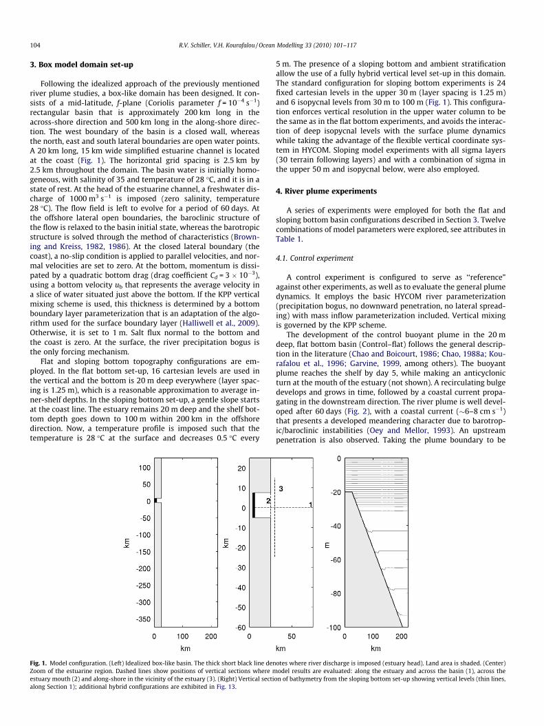
Following the idealized approach of the previously mentionedriver plume studies, a box-like domain has been designed. It con-sists of a mid-latitude, f-plane (Coriolis parameter f = 10�4 s�1)rectangular basin that is approximately 200 km long in theacross-shore direction and 500 km long in the along-shore direc-tion. The west boundary of the basin is a closed wall, whereasthe north, east and south lateral boundaries are open water points.A 20 km long, 15 km wide simplified estuarine channel is locatedat the coast (Fig. 1). The horizontal grid spacing is 2.5 km by2.5 km throughout the domain. The basin water is initially homo-geneous, with salinity of 35 and temperature of 28 �C, and it is in astate of rest. At the head of the estuarine channel, a freshwater dis-charge of 1000 m3 s�1 is imposed (zero salinity, temperature28 �C). The flow field is left to evolve for a period of 60 days. Atthe offshore lateral open boundaries, the baroclinic structure ofthe flow is relaxed to the basin initial state, whereas the barotropicstructure is solved through the method of characteristics (Brown-ing and Kreiss, 1982, 1986). At the closed lateral boundary (thecoast), a no-slip condition is applied to parallel velocities, and nor-mal velocities are set to zero. At the bottom, momentum is dissi-pated by a quadratic bottom drag (drag coefficient Cd = 3 � 10�3),using a bottom velocity ub that represents the average velocity ina slice of water situated just above the bottom. If the KPP verticalmixing scheme is used, this thickness is determined by a bottomboundary layer parameterization that is an adaptation of the algo-rithm used for the surface boundary layer (Halliwell et al., 2009).Otherwise, it is set to 1 m. Salt flux normal to the bottom andthe coast is zero. At the surface, the river precipitation bogus isthe only forcing mechanism.

Flat and sloping bottom topography configurations are em-ployed. In the flat bottom set-up, 16 cartesian levels are used inthe vertical and the bottom is 20 m deep everywhere (layer spac-ing is 1.25 m), which is a reasonable approximation to average in-ner-shelf depths. In the sloping bottom set-up, a gentle slope startsat the coast line. The estuary remains 20 m deep and the shelf bot-tom depth goes down to 100 m within 200 km in the offshoredirection. Now, a temperature profile is imposed such that thetemperature is 28 �C at the surface and decreases 0.5 �C every

Fig. 1. Model configuration. (Left) Idealized box-like basin. The thick short black line denZoom of the estuarine region. Dashed lines show positions of vertical sections where mestuary mouth (2) and along-shore in the vicinity of the estuary (3). (Right) Vertical sectialong Section 1); additional hybrid configurations are exhibited in Fig. 13.

5 m. The presence of a sloping bottom and ambient stratificationallow the use of a fully hybrid vertical level set-up in this domain.The standard configuration for sloping bottom experiments is 24fixed cartesian levels in the upper 30 m (layer spacing is 1.25 m)and 6 isopycnal levels from 30 m to 100 m (Fig. 1). This configura-tion enforces vertical resolution in the upper water column to bethe same as in the flat bottom experiments, and avoids the interac-tion of deep isopycnal levels with the surface plume dynamicswhile taking the advantage of the flexible vertical coordinate sys-tem in HYCOM. Sloping model experiments with all sigma layers(30 terrain following layers) and with a combination of sigma inthe upper 50 m and isopycnal below, were also employed.

4. River plume experiments

A series of experiments were employed for both the flat andsloping bottom basin configurations described in Section 3. Twelvecombinations of model parameters were explored, see attributes inTable 1.

4.1. Control experiment

A control experiment is configured to serve as ‘‘reference”against other experiments, as well as to evaluate the general plumedynamics. It employs the basic HYCOM river parameterization(precipitation bogus, no downward penetration, no lateral spread-ing) with mass inflow parameterization included. Vertical mixingis governed by the KPP scheme.

The development of the control buoyant plume in the 20 mdeep, flat bottom basin (Control–flat) follows the general descrip-tion in the literature (Chao and Boicourt, 1986; Chao, 1988a; Kou-rafalou et al., 1996; Garvine, 1999, among others). The buoyantplume reaches the shelf by day 5, while making an anticyclonicturn at the mouth of the estuary (not shown). A recirculating bulgedevelops and grows in time, followed by a coastal current propa-gating in the downstream direction. The river plume is well devel-oped after 60 days (Fig. 2), with a coastal current (�6–8 cm s�1)that presents a developed meandering character due to barotrop-ic/baroclinic instabilities (Oey and Mellor, 1993). An upstreampenetration is also observed. Taking the plume boundary to be

otes where river discharge is imposed (estuary head). Land area is shaded. (Center)odel results are evaluated: along the estuary and across the basin (1), across the

on of bathymetry from the sloping bottom set-up showing vertical levels (thin lines,

Table 1Summary of the attributes from the study experiments. Downward penetration isgiven in percentage of the water column and in meters (parentheses). Lateralspreading is classified as none, short (4 grid points, half-estuary length) or large (7grid points, full-estuary length). KPP background vertical mixing is characterized asstandard (no modifications) or as Enhanced Kiw (salinity diffusivity due to backgroundinternal wave mixing equals 10�4 m2 s�1) plus region where it is applied. See Sections4.2 and 4.3 for details.

Experiment Downwardpenetration (pntr)

Lateralspreading (sprd)

KPP backgroundvertical mixing

Control 0% (0) None StandardRiv1b 20% (4) None StandardRiv1c 40% (8) None StandardRiv2a 0% (0) Short StandardRiv2b 20% (4) Short StandardRiv2c 40% (8) Short StandardRiv3a 0% (0) Large StandardRiv3b 20% (4) Large StandardRiv3c 40% (8) Large StandardMix4a 0% (0) None Enhanced Kiw at

the estuary headMix4b 0% (0) None Enhanced Kiw over

half-estuary lengthMix4c 0% (0) None Enhanced Kiw over

full-estuary length


the 34.9 salinity isoline, the nose of the coastal current has reached202.5 km south of the river mouth. The offshore extension of thebulge (72.5 km) is larger than the coastal current width(62.5 km), which represents a supercritical plume case (Chao,1988a). A weaker undercurrent (not shown) runs in the upstreamdirection opposite to the downstream coastal current below 6–8 m, with velocities around 3 cm s�1. An across-shore vertical sec-tion of salinity contours (Fig. 2) shows that the buoyant flow formsa 2-layer structure, with a surface buoyant layer on top of denserambient water. This is the case of a surface-advected plume (Yan-kovsky and Chapman, 1997), which presents a recirculating bulge,a coastal current close to the coast and very little contact with thebottom. The maximum barotropic velocity at the bulge reaches3 cm s�1, well below the maximum baroclinic velocity (12 cm s�1).

In sloping bottom conditions (Control–slope, Fig. 3), the plumedevelops a recirculating bulge that is elongated in the upstreamdirection and shortened in the offshore direction in comparison to

Fig. 2. (Upper) Sea Surface Height contours in mm (SSH, left), Sea Surface Salinity contouflat experiment at day 60 (part of the model domain shown). (Lower) Along-estuary/acboundary (34.9) is represented by a white line. Salinity values less than 25 (inside the es

Control–flat. An enhanced upstream intrusion develops, as most ofthe buoyant outflow turns to the left upon exiting the estuary, beforeturning anticyclonically and merging to the coastal current (whichexhibits less meandering). The enhancement of the upstream andshortening of the offshore intrusions have been reported in previousstudies (Kourafalou et al., 1996; Garvine, 1999), and the changes inthe bulge structure suggest the effect of potential vorticity con-strains imposed by the bottom slope (Chao, 1988a).

4.2. Prescribed river inflow distributions inside the estuary

We examine changes in the development and structure of theriver plume when the river inflow distribution is prescribed insidethe estuary. This is accomplished by employing the river parame-terization options of enhanced downward penetration and hori-zontal spreading of the river inflow (described in Section 2.1),which effectively change the vertical and horizontal mixing ofthe buoyant plume at the source. This redistribution of freshwaterinput is expected to change the properties of the buoyant outflowat the estuary mouth and impact the development of the riverplume in the receiving basin. We enhance the downward penetra-tion of the river inflow to 20% (4 m) and 40% (8 m) of the water col-umn and impose a short lateral spreading (half the estuary length)and a large lateral spreading (the entire estuary length). Togetherwith the Control case, nine different parameter combinations forthe study experiments are employed (Table 1); ‘‘experiment(s)”will be abbreviated ‘‘expt(s)” thereafter. All expts in this group em-ploy the KPP vertical mixing scheme. Snapshots of the plume SeaSurface Salinity (SSS) and the bulge near surface velocity vectors(both at day 60) are presented in Figs. 4 and 5, respectively. Theextensions of each plume upstream (Lu), downstream (Ld) and off-shore (Lo) intrusions are also depicted in Fig. 4.

4.2.1. Variable downward penetration and no lateral spreadingCases of variable downward penetration (0%, 20% and 40%) with

no lateral spreading of the river inflow are shown in Fig. 4 (upperpanels). There is a considerable change in the shape and extensionof the plume when the downward penetration of the river dis-charge is enhanced to 20% (expt Riv1b–flat); the anticyclonic bulgegrows in size, with a larger offshore extension and a more circular

rs (SSS, middle) and near surface velocity vectors in cm s�1 (right) from the Control–ross-shore salinity vertical structure along Section 1 (marked in Fig. 1). The plumetuary) are not shown. Vertical black line denotes the position of the estuary mouth.

Fig. 3. As Fig. 2, but for the Control–slope experiment.


shape. A stronger coastal current is present, with more meandersand a longer downstream extension. Interestingly, the upstreampenetration is much reduced. This pattern is enhanced when thismixing is forced down to 40% of the water column (Riv1c–flat).In all cases, the buoyant outflow is denser with increasing down-ward penetration of the inflowing river discharge. The surface cir-culation from these experiments (Fig. 5, upper panels)demonstrates a progressive strengthening of the buoyant outflowwith increasing downward penetration of the river inflow by 20%(Riv1b–flat) and 40% (Riv1c–flat). A shift in the position and direc-tion of the estuary outflow is also observed, which has clear impacton the shape and location of the offshore bulge. The plume outflowis concentrated in the northern wall of the estuary mouth and exitsin a straight path (Control–flat), and as it intensifies it spreadsacross the estuary mouth (Riv1b–flat) and develops an enhancedanticyclonic turning (Riv1c–flat).

The effect of the bottom slope is demonstrated on the Riv1ccase, depicting a marked impact on both the estuary outflow andthe bulge development (Riv1c–slope, Figs. 4 and 5). In this casethe buoyant outflow does not present an anticyclonic veering, asit exits the estuary in a straight path (similar to Control–slope).The bulge presents a marked upstream displacement and upstreamflow intrusion, which are accompanied by a shorter offshore ex-tent. As the bottom slope ‘‘squeezes” the buoyant flow area againstthe coast, the plume is elongated in the along-shore direction anddevelops a longer coastal current region.

4.2.2. Variable downward penetration and short lateral spreadingThe general pattern in the surface salinity field discussed above

(reduction of the upstream intrusion, larger offshore bulge andlarger downstream penetration) is also observed when the down-ward penetration of the river inflow is increased in the presenceof short lateral spreading (Fig. 4, middle panels). However, somedistinctions from the same cases with no lateral spreading are ob-served. The upstream intrusion enhances from the expt Control–flat to Riv2a–flat and the bulge is slightly less circular in expt

Riv2b–flat than in Riv1b–flat. No major changes are observed inthe salinity field from expts Riv1c–flat and Riv2c–flat, except theoutflow from Riv2c–flat is less buoyant and the bulge is largerthan in experiment Riv1c–flat. The general pattern of buoyantoutflow intensification and development of an anticyclonic veer-ing is also observed when downward penetration increases from0 to 40% (Fig. 5, middle panels). Finally, the trend imposed bythe bottom slope in expt Riv1c–slope is also observed in Riv2c–slope, where the bulge is displaced in the upstream direction,the outflow does not develop an anticyclonic veering and thecoastal current region is elongated.

4.2.3. Variable downward penetration and large lateral spreadingThe plume surface salinity field changed considerably when the

vertical penetration of the river inflow was varied while employinglarge spreading (Figs. 4 and 5, lower panels), as now both verticaland horizontal salinity gradients were impacted. The same patternof enhancement of the upstream intrusion is observed at 0% down-ward penetration (Riv3a–flat), which vanishes at 20% downwardpenetration (Riv3b–flat) as the bulge becomes less circular and lessdistinct from the coastal current (in comparison to Riv2b–flat). Thelargest changes in plume shape were observed at 40% downwardpenetration (Riv3c–flat), when the offshore bulge did not developand the plume turned abruptly to the right and moved down-stream forming a coastal current that started unidirectional andthen developed a meandering pattern, starting with a featureresembling a secondary bulge due to the large amount of low salin-ity water that has leaked along the coast. The near surface velocityfield (Fig. 5, lower panels) confirms that the outflow from exptRiv3c–flat developed an abrupt right turn at the estuary mouthand all plume waters were deflected southward, increasing thedownstream coastal current penetration. Conversely, the develop-ment of the plume in sloping bottom conditions (Riv3c–slope) isconsiderably different as an offshore bulge develops in front ofthe estuary, the buoyant outflow exits in a straight path and aslight upstream intrusion is observed. The presence of a slope ap-

Fig. 4. Sea Surface Salinity contours from experiments with variable distribution of river inflow inside the estuary, at day 60 (part of the model domain shown). The plumeboundary (34.9) is represented by a white line. Salinity values less than 25 (inside the estuary) are not shown. The upstream (Lu), downstream (Ld) and offshore (Lo) plumeintrusions for each case are displayed next to the plots. Downward penetration (pntr) and horizontal spreading (sprd) configurations that characterize each experiment arealso presented.


pears to overwhelm the impact of lateral and/or vertical mixing in-side the estuary, as suggested by the similarities of the Riv2c–slopeand Riv3c–slope expts, in contrast to their clearly different flat bot-tom counterparts.

4.3. Enhanced vertical mixing inside the estuary

The impact of changes in the vertical mixing at the freshwatersource on the development of the river plume is also investigated.Instead of mixing the river freshwater by redistributing it, thebackground mixing within the KPP vertical mixing scheme wasenhanced. Specifically, the vertical salinity diffusivity due to back-ground internal wave mixing Kiw was increased to 10�4 m2 s�1 (10times its standard background value) inside the estuary. Threeexpts were performed, where Kiw was enhanced in three distinctregions: at the estuary head, from the head to half the estuarylength and from the head to the estuary mouth (full-estuarylength). The choice to change Kiw and not other aspects of theKPP vertical mixing scheme was based on the fact that the back-ground internal wave mixing is the main contributor to verticalmixing in the study experiments (see discussion below). In orderto access the sensitivity of the plume structure to the choice of

vertical mixing scheme, twin expts of the Control–flat case thatemploy the MY2.5 and GISS vertical mixing schemes wereperformed.

The enhancement of Kiw inside the estuary effectively impactsthe outflow properties and the development of the buoyant plume.SSS and near surface velocity vectors from this group of experi-ments (Fig. 6) demonstrate that as the estuarine region was mixedthrough enhanced Kiw, the outflow became less fresh, progressivelydeveloped an anticyclonic turning and decreased the plume up-stream penetration. The offshore bulge was clearly impacted bythose changes, as it is shown to shift downstream and finally van-ish with the outflow being deflected in the downstream direction.The surface fields from the half-estuary (Mix4b–flat) and full-estu-ary (Mix4c–flat) cases resemble those impacted by 40% downwardpenetration at short (Riv2c–flat) and large (Riv3c–flat) horizontalspreading, respectively. In the presence of the bottom slope(Mix4c–slope), the plume evolves to the same structure as in theexpt Riv3c–slope.

The mixing expts revealed that the plume structure was not sen-sitive to the choice of vertical mixing schemes. Employing the MY2.5or the GISS vertical mixing schemes produced river plumes that hadthe same vertical salinity structure as the Control experiment (KPP),

Fig. 5. Near surface velocity vectors from experiments with variable distribution of river inflow inside the estuary, at day 60 (part of the model domain shown). Downwardpenetration (pntr) and horizontal spreading (sprd) configurations that characterize each experiment are presented. Vectors are plotted every other grid point for bettervisualization.


as well as the SSS and near surface currents (not shown). This findingsuggests that the vertical eddy mixing coefficients computed by eachscheme are approximately the same and that vertical mixing is beingcontrolled by the same process. In this study, two common compo-nents of the ocean interior mixing should be important: the unre-solved background internal wave mixing and shear instability. InHYCOM and for all vertical mixing schemes employed here, thebackground internal wave mixing is parameterized through con-stant coefficients: scalar diffusivity is equal to 10�5 m2 s�1, whereasbackground viscosity is 10�4 m2 s�1. The parameterization of shear-driven mixing depends on the choice of vertical mixing scheme, butit is commonly related to a critical Richardson number below whichthe parameterization is activated. The Richardson number at modelinterfaces from the experiments with the three different verticalmixing schemes was calculated and compared to the Richardsonnumber threshold from each scheme (not shown). All values of thecalculated Richardson number within the buoyant plume wereabove the critical value below which mixing occurs, which suggeststhat in the study experiments the parameterization of shear-in-duced mixing is not triggered for any choice of scheme, and thatthe buoyant plume vertical mixing is controlled by the backgroundinternal wave parameterization.

5. Discussion of results

5.1. Variability of outflow properties

Enhanced vertical and horizontal mixing of the river inflow in-side the estuary impacted the river mouth conditions and thestructure of the buoyant outflow. Fig. 7 shows across-estuary sec-tions (along Section 2 at the estuary mouth, see Fig. 1) of Sea Sur-face Height (SSH), salinity and along-estuary (u) velocity forselected experiments, at day 60. As expected, progressivelyincreasing the downward penetration of the river inflow (Riv2-a,b,c–flat) or enlarging the estuary area with enhanced Kiw (Mix-a,b,c–flat) generated plume outflows that were deeper anddenser. A coupled upper outflow/lower inflow structure is ob-served, which represents the classic gravitational circulation veri-fied in previous numerical studies (Chao, 1988a). Thisgravitational circulation was enhanced as the mixing of river in-flow inside the estuary increased, and the upper outflow and bot-tom inflow increased in magnitude. This effectively enhanced theoutflow transport Tf ¼

RAf

udAf (Af is the upper outflow area whereu is positive, see Fig. 7 for selected expts and Table 2 for all flat bot-tom expts). Tf increased 146% from Riv2a to Riv2b, 55% from Riv2b

Fig. 6. Sea Surface Salinity contours (upper) and near surface velocity vectors (lower) from experiments with enhanced mixing (increased Kiw) inside the estuary, at day 60(part of the model domain shown). The plume boundary (34.9) is represented by a white line. Salinity values less than 25 (inside the estuary) are not shown. The mixinginformation that characterizes each experiment is shown next to each plot (see Section 4.3 for details). Vectors are plotted every other grid point for better visualization.


to Riv2c, 70% from Mix4a to Mix4b and 18% from Mix4b to Mix 4c.All other ‘‘Riv” flat bottom cases present increases in Tf that are ofthe same order as in expts Riv2a,b,c–flat. Across-estuary (v) veloc-ity distributions (not shown) demonstrate the development of aveering pattern of the plume outflow, which intensifies as freshwa-ter mixing inside the estuary is enhanced. The above changes wereaccompanied by a progressive steepening of the salinity isolines,which was also followed by a slight steepening of the across-estu-ary SSH. The plume vertical structure suggests that the outflow isin geostrophic balance, which is strengthened with enhanced mix-ing of riverine waters inside the estuary. The presence of a bottomslope in the basin also impacted the vertical structure of the out-flow. As the outflow shifted to the north side of the estuary mouth,the low-salinity area was enlarged and the isopycnals and SSH be-came flatter on the south side of the mouth (Riv2c–slope andMix4c–slope). The plume outflow structure of the Control–slopecase is the same as in the presence of a flat bottom. Interestingly,the slope experiments presented smaller Tf in comparison to theirflat bottom counterparts (Fig. 7), which suggests a two-way inter-action between the dynamics of the buoyant flow in the estuaryand in the receiving basin (in Fig. 7, a comparison between Con-trol–slope and Riv2a–flat is valid because the plume does not reallychange from the Riv2a–flat to the Control–flat case).

In order to summarize the main geophysical properties of thedifferent outflows, we calculated common non-dimensional num-bers from all flat bottom experiments. We concentrated on the flatbottom expts, as they facilitate comparisons to 2-layer analyticalmodels. Such calculations involved an approximation of the plumeoutflow to a two-layer formulation defined by hr, the depth wherethe along-estuary velocity (u) becomes negative. We defined anoutflow upper layer with thickness h1, density q1 and velocitiesu1 and v1, and an inflow lower layer with thickness h2, density q2

and velocities u2 and v2. For each experiment, vertical profiles ofu, v and q were extracted at the location of the core of the surfaceoutflow at the estuary mouth; q1, q2, u1, u2, v1 and v2 were calcu-

lated as vertical mean values from the model grid points that arewithin each layer h1 and h2 (above and below hr, respectively)and are presented in Table 2. These calculations did not involveaverages in the across-estuary direction because in some casesthe outflow velocity field is clearly concentrated on one side ofthe estuary channel and an average in the y direction would under-estimate the outflow velocity. We calculated the gradient Richard-son number Ri ¼ N2=S2, the Froude number Fr ¼ j~V1j=ci, the inletRossby number Roi ¼ j~V1j=ðfWÞ and the inlet Kelvin numberKi ¼W=Rdi. N2 ¼ ð�g=q0Þðq1 � q2Þ=Dz is the squared stratificationfrequency, S2 ¼ ðu1 � u2=DzÞ2 þ ðv1 � v2=DzÞ2 is the squared veloc-ity vertical shear, ci ¼

ffiffiffiffiffiffiffiffiffiffiffiffiffiffiffiffiffiffiffiffiffiffiffiffiffiffiffiffiffiffiffiffiffiffiffiffiffiffiffiffiffiffiffiffiffiffiffig0ðh1 � h2Þ=ðh1 þ h2Þ

pis the phase speed of

long internal gravity waves and Rdi ¼ ci=f is the internal radius ofdeformation; g0 ¼ g � ðq2 � q1Þ=q0 is the reduced gravity, g isthe gravitational acceleration (9.806 m s�2), qo is the initial ambi-ent density (1022.40 kg m�3), Dz is the distance from the surface(z = 0, axis positive upwards) down to the interface of the layers(equal to h1); j~V1j is the length of the upper layer velocity vector,W is the estuary width (15 km) and f is the Coriolis parameter(10�4 s�1).

The non-dimensional numbers presented in Table 3 summarizeand corroborate with the properties of the distinct outflows. Ki waslarger than 1 in all experiments, which indicates that the studyexperiments are all large scale discharges and that the dynamicsat the estuary mouth are affected by the earth’s rotation. The factthat Roi is smaller than 1 in all experiments suggests that advectionplays a secondary role in the dynamics governing the immediatevicinity of the estuary outflow. The outflows should be approxi-mately in geostrophic balance, which is in agreement with thesalinity vertical structures presented in Fig. 7 and will be exploredfurther in the next section. Considerably large Ri (>20) was foundin experiments that did not have enhanced vertical mixing of theriver inflow (expts Control–flat, Riv2a,3a–flat), and progressivelydecreased to values below 3 (expts Riv2c,3c–flat and Mix4c–flat)as we enhanced vertical mixing (via downward penetration or lar-

Fig. 7. Sea Surface Height (SSH, in mm), across-estuary salinity vertical structure (colors) and along-estuary velocity (u, cm s�1, solid for positive/offshore and dashed fornegative/onshore contours) along Section 2 (estuary mouth) from selected experiments, at day 60. The configurations that define each experiment and the outflow transportTf for each case are shown. Salinity values less than 25 are not shown.

Table 2Outflow transport Tf, outflow upper layer 1 and inflow lower layer 2 vertical mean values of density q, along-estuary (u) and across-estuary (v) velocities and layer thickness h, forall flat bottom experiments at day 60. Layers 1 and 2 average values were calculated from a vertical profile located at the core of the surface outflow at the estuary mouth. SeeTable 1 for attributes from experiments and Section 5.1 for details on the calculations.

Experiment Tf (m3 s�1 � 103) q1 (sigma) u1 (m s�1) v1 (m s�1) h1 (m) q2 (sigma) u2 (m s�1) v2 (m s�1) h2 (m)

Control 2.7 19.95 0.06 0.01 6.25 22.33 �0.02 0.00 13.75Riv1b 6.1 20.64 0.09 �0.02 6.25 22.37 �0.03 0.00 15.00Riv1c 9.0 20.33 0.12 �0.05 7.50 22.25 �0.05 0.00 12.50Riv2a 2.7 19.54 0.06 0.01 6.25 22.32 �0.02 0.00 13.75Riv2b 6.8 20.54 0.12 �0.04 5.00 22.34 �0.03 0.00 15.00Riv2c 10.5 20.59 0.13 �0.14 7.50 22.25 �0.05 0.00 12.50Riv3a 2.7 19.41 0.06 0.01 6.25 22.32 �0.02 0.00 13.75Riv3b 6.6 19.67 0.13 �0.03 5.00 22.30 �0.04 0.01 15.00Riv3c 11.1 20.96 0.10 �0.05 8.75 22.31 �0.08 0.04 11.25Mix4a 4.1 19.84 0.08 0.01 7.50 22.32 �0.03 0.00 12.50Mix4b 7.0 20.69 0.10 �0.08 6.25 22.35 �0.03 0.00 13.75Mix4c 8.3 21.09 0.10 �0.06 6.25 22.32 �0.05 0.02 13.75


ger Kiw). As expected, this was followed by an opposite behavior ofFr. Vertical stratification is important to the flow dynamics (allcases presented Fr less than one) and Fr increases with increasingdownward penetration, meaning that the importance of stratifica-

tion (here measured by ci) decreases relative to the horizontaladvection of the flow. All cases fall in the category of large scalebuoyant flows (Garvine, 1995) which are characterized by largeKi, small Roi and small Fr.

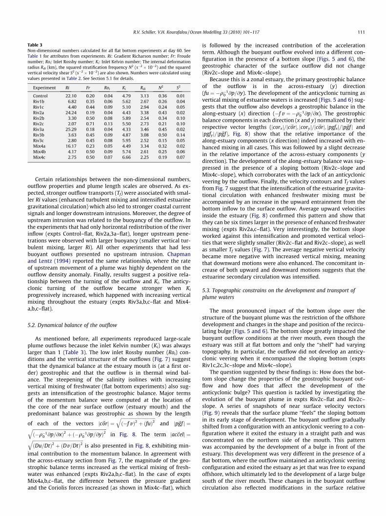
Table 3Non-dimensional numbers calculated for all flat bottom experiments at day 60. SeeTable 1 for attributes from experiments. Ri: Gradient Richarson number; Fr: Froudenumber; Roi: Inlet Rossby number; Ki: Inlet Kelvin number; The internal deformationradius Rdi (km), the squared stratification frequency N2 (s�2 � 10�2) and the squaredvertical velocity shear S2 (s�2 � 10�2) are also shown. Numbers were calculated usingvalues presented in Table 2. See Section 5.1 for details.

Experiment Ri Fr Roi Ki Rdi N2 S2

Control 22.10 0.20 0.04 4.79 3.13 0.36 0.01Riv1b 6.82 0.35 0.06 5.62 2.67 0.26 0.04Riv1c 4.40 0.44 0.09 5.10 2.94 0.24 0.05Riv2a 24.24 0.19 0.04 4.43 3.38 0.43 0.02Riv2b 3.30 0.50 0.08 5.89 2.54 0.34 0.10Riv2c 2.07 0.71 0.13 5.50 2.73 0.21 0.10Riv3a 25.29 0.18 0.04 4.33 3.46 0.45 0.02Riv3b 3.63 0.45 0.09 4.87 3.08 0.50 0.14Riv3c 2.80 0.45 0.08 5.95 2.52 0.15 0.05Mix4a 16.17 0.23 0.05 4.49 3.34 0.32 0.02Mix4b 4.17 0.50 0.09 5.74 2.61 0.25 0.06Mix4c 2.75 0.50 0.07 6.66 2.25 0.19 0.07


Certain relationships between the non-dimensional numbers,outflow properties and plume length scales are observed. As ex-pected, stronger outflow transports (Tf) were associated with smal-ler Ri values (enhanced turbulent mixing and intensified estuarinegravitational circulation) which also led to stronger coastal currentsignals and longer downstream intrusions. Moreover, the degree ofupstream intrusion was related to the buoyancy of the outflow. Inthe experiments that had only horizontal redistribution of the riverinflow (expts Control–flat, Riv2a,3a–flat), longer upstream pene-trations were observed with larger buoyancy (smaller vertical tur-bulent mixing, larger Ri). All other experiments that had lessbuoyant outflows presented no upstream intrusion. Chapmanand Lentz (1994) reported the same relationship, where the rateof upstream movement of a plume was highly dependent on theoutflow density anomaly. Finally, results suggest a positive rela-tionship between the turning of the outflow and Ki. The anticy-clonic turning of the outflow became stronger when Ki

progressively increased, which happened with increasing verticalmixing throughout the estuary (expts Riv3a,b,c–flat and Mix4-a,b,c–flat).

5.2. Dynamical balance of the outflow

As mentioned before, all experiments reproduced large-scaleplume outflows because the inlet Kelvin number (Ki) was alwayslarger than 1 (Table 3). The low inlet Rossby number (Roi) con-ditions and the vertical structure of the outflows (Fig. 7) suggestthat the dynamical balance at the estuary mouth is (at a first or-der) geostrophic and that the outflow is in thermal wind bal-ance. The steepening of the salinity isolines with increasingvertical mixing of freshwater (flat bottom experiments) also sug-gests an intensification of the geostrophic balance. Major termsof the momentum balance were computed at the location ofthe core of the near surface outflow (estuary mouth) and thepredominant balance was geostrophic as shown by the length

of each of the vectors jc~orj ¼ffiffiffiffiffiffiffiffiffiffiffiffiffiffiffiffiffiffiffiffiffiffiffiffiffiffiffiffiffiffiffið�fvÞ2 þ ðfuÞ2

qand jp~gf j ¼ffiffiffiffiffiffiffiffiffiffiffiffiffiffiffiffiffiffiffiffiffiffiffiffiffiffiffiffiffiffiffiffiffiffiffiffiffiffiffiffiffiffiffiffiffiffiffiffiffiffiffiffiffiffiffiffiffiffiffiffiffiffiffiffiffiffiffi

ð�q�10 @p=@xÞ2 þ ð�q�1

0 @p=@yÞ2q

in Fig. 8. The term jac~celj ¼ffiffiffiffiffiffiffiffiffiffiffiffiffiffiffiffiffiffiffiffiffiffiffiffiffiffiffiffiffiffiffiffiffiffiffiffiffiffiffiffiffiffiffiffiffiffiðDu=DtÞ2 þ ðDv=DtÞ2

qis also presented in Fig. 8, exhibiting min-

imal contribution to the momentum balance. In agreement withthe across-estuary section from Fig. 7, the magnitude of the geo-strophic balance terms increased as the vertical mixing of fresh-water was enhanced (expts Riv2a,b,c–flat). In the case of exptsMix4a,b,c–flat, the difference between the pressure gradientand the Coriolis forces increased (as shown in Mix4c–flat), which

is followed by the increased contribution of the accelerationterm. Although the buoyant outflow evolved into a different con-figuration in the presence of a bottom slope (Figs. 5 and 6), thegeostrophic character of the surface outflow did not change(Riv2c–slope and Mix4c–slope).

Because this is a zonal estuary, the primary geostrophic balanceof the outflow is in the across-estuary (y) direction(fu ¼ �q�1

0 @p=@y). The development of the anticyclonic turning asvertical mixing of estuarine waters is increased (Figs. 5 and 6) sug-gests that the outflow also develops a geostrophic balance in thealong-estuary (x) direction (�f v ¼ �q�1

0 @p=@x). The geostrophicbalance components in each direction (x and y) normalized by theirrespective vector lengths (jcorxj=jc~orj; jcoryj=jc~orj; jpgfxj=jp~gf j andjpgfyj=jp~gf j, Fig. 8) show that the relative importance of thealong-estuary components (x direction) indeed increased with en-hanced mixing in all cases. This was followed by a slight decreasein the relative importance of the across-estuary components (ydirection). The development of the along-estuary balance was sup-pressed in the presence of a sloping bottom (Riv2c–slope andMix4c–slope), which corroborates with the lack of an anticyclonicveering by the outflow. Finally, the velocity contours and Tf valuesfrom Fig. 7 suggest that the intensification of the estuarine gravita-tional circulation with enhanced freshwater mixing must beaccompanied by an increase in the upward entrainment from thebottom inflow to the surface outflow. Average upward velocitiesinside the estuary (Fig. 8) confirmed this pattern and show thatthey can be six times larger in the presence of enhanced freshwatermixing (expts Riv2a,c–flat). Very interestingly, the bottom slopeworked against this intensification and promoted vertical veloci-ties that were slightly smaller (Riv2c–flat and Riv2c–slope), as wellas smaller Tf values (Fig. 7). The average negative vertical velocitybecame more negative with increased vertical mixing, meaningthat downward motions were also enhanced. The concomitant in-crease of both upward and downward motions suggests that theestuarine secondary circulation was intensified.

5.3. Topographic constrains on the development and transport ofplume waters

The most pronounced impact of the bottom slope over thestructure of the buoyant plume was the restriction of the offshoredevelopment and changes in the shape and position of the recircu-lating bulge (Figs. 5 and 6). The bottom slope greatly impacted thebuoyant outflow conditions at the river mouth, even though theestuary was still at flat bottom and only the ‘‘shelf” had varyingtopography. In particular, the outflow did not develop an anticy-clonic veering when it encompassed the sloping bottom (exptsRiv1c,2c,3c–slope and Mix4c–slope).

The question suggested by these findings is: How does the bot-tom slope change the properties of the geostrophic buoyant out-flow and how does that affect the development of theanticyclonic bulge? This question is tackled by investigating theevolution of the buoyant plume in expts Riv2c–flat and Riv2c–slope. A series of snapshots of near surface velocity vectors(Fig. 9) reveals that the surface plume ‘‘feels” the sloping bottomin its early stage of development. The buoyant outflow graduallyshifted from a configuration with an anticyclonic veering to a con-figuration where it exited the estuary in a straight path and wasconcentrated on the northern side of the mouth. This patternwas accompanied by the development of a bulge in front of theestuary. This development was very different in the presence of aflat bottom, where the outflow maintained an anticyclonic veeringconfiguration and exited the estuary as jet that was free to expandoffshore, which ultimately led to the development of a large bulgesouth of the river mouth. These changes in the buoyant outflowcirculation also reflected modifications in the surface relative

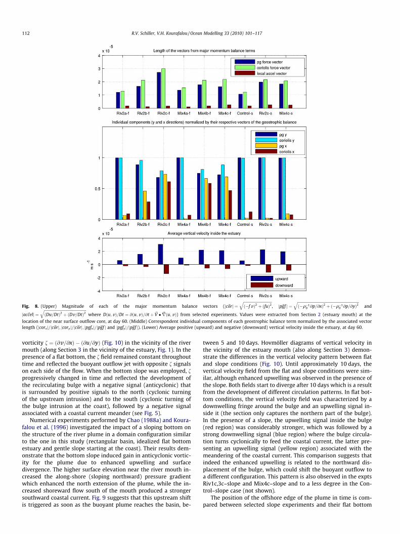
Fig. 8. (Upper) Magnitude of each of the major momentum balance vectors (jc~orj ¼ffiffiffiffiffiffiffiffiffiffiffiffiffiffiffiffiffiffiffiffiffiffiffiffiffiffiffiffiffiffiffið�f vÞ2 þ ðfuÞ2

q, jp~gf j ¼

ffiffiffiffiffiffiffiffiffiffiffiffiffiffiffiffiffiffiffiffiffiffiffiffiffiffiffiffiffiffiffiffiffiffiffiffiffiffiffiffiffiffiffiffiffiffiffiffiffiffiffiffiffiffiffiffiffiffiffiffiffiffiffiffiffiffiffið�q�1

0 @p=@xÞ2 þ ð�q�10 @p=@yÞ2

qand

jac~celj ¼ffiffiffiffiffiffiffiffiffiffiffiffiffiffiffiffiffiffiffiffiffiffiffiffiffiffiffiffiffiffiffiffiffiffiffiffiffiffiffiffiffiffiffiffiffiffiðDu=DtÞ2 þ ðDv=DtÞ2

qwhere Dðu;vÞ=Dt ¼ @ðu; vÞ=@t þ ~V � ~rðu; vÞ) from selected experiments. Values were extracted from Section 2 (estuary mouth) at the

location of the near surface outflow core, at day 60. (Middle) Correspondent individual components of each geostrophic balance term normalized by the associated vectorlength (jcorxj=jc~orj; jcoryj=jc~orj; jpgfxj=jp~gf j and jpgfyj=jp~gf j). (Lower) Average positive (upward) and negative (downward) vertical velocity inside the estuary, at day 60.


vorticity f ¼ ð@v=@xÞ � ð@u=@yÞ (Fig. 10) in the vicinity of the rivermouth (along Section 3 in the vicinity of the estuary, Fig. 1). In thepresence of a flat bottom, the f field remained constant throughouttime and reflected the buoyant outflow jet with opposite f signalson each side of the flow. When the bottom slope was employed, fprogressively changed in time and reflected the development ofthe recirculating bulge with a negative signal (anticyclonic) thatis surrounded by positive signals to the north (cyclonic turningof the upstream intrusion) and to the south (cyclonic turning ofthe bulge intrusion at the coast), followed by a negative signalassociated with a coastal current meander (see Fig. 5).

Numerical experiments performed by Chao (1988a) and Koura-falou et al. (1996) investigated the impact of a sloping bottom onthe structure of the river plume in a domain configuration similarto the one in this study (rectangular basin, idealized flat bottomestuary and gentle slope starting at the coast). Their results dem-onstrate that the bottom slope induced gain in anticyclonic vortic-ity for the plume due to enhanced upwelling and surfacedivergence. The higher surface elevation near the river mouth in-creased the along-shore (sloping northward) pressure gradientwhich enhanced the north extension of the plume, while the in-creased shoreward flow south of the mouth produced a strongersouthward coastal current. Fig. 9 suggests that this upstream shiftis triggered as soon as the buoyant plume reaches the basin, be-

tween 5 and 10 days. Hovmöller diagrams of vertical velocity inthe vicinity of the estuary mouth (also along Section 3) demon-strate the differences in the vertical velocity pattern between flatand slope conditions (Fig. 10). Until approximately 10 days, thevertical velocity field from the flat and slope conditions were sim-ilar, although enhanced upwelling was observed in the presence ofthe slope. Both fields start to diverge after 10 days which is a resultfrom the development of different circulation patterns. In flat bot-tom conditions, the vertical velocity field was characterized by adownwelling fringe around the bulge and an upwelling signal in-side it (the section only captures the northern part of the bulge).In the presence of a slope, the upwelling signal inside the bulge(red region) was considerably stronger, which was followed by astrong downwelling signal (blue region) where the bulge circula-tion turns cyclonically to feed the coastal current, the latter pre-senting an upwelling signal (yellow region) associated with themeandering of the coastal current. This comparison suggests thatindeed the enhanced upwelling is related to the northward dis-placement of the bulge, which could shift the buoyant outflow toa different configuration. This pattern is also observed in the exptsRiv1c,3c–slope and Mix4c–slope and to a less degree in the Con-trol–slope case (not shown).

The position of the offshore edge of the plume in time is com-pared between selected slope experiments and their flat bottom

Fig. 9. Snapshots of near surface velocity vectors from Riv2c experiments (from both flat and sloping bottom conditions) starting on day 5 to day 30, every 5 days (part of themodel domain shown). Vectors are plotted every other grid point for better visualization.


counterparts (Fig. 11). Apart from the Control cases, the recirculat-ing bulges in flat and sloping bottom conditions started to divergefrom each other around day 15 and the bottom slope imposed sig-nificant upstream displacements of the bulge after 60 days. Theabove changes in the recirculating bulge also impacted coastal cur-rent properties such as the displacement of the coastal currentnose and the integrated transport (m3 s�1), which is defined asthe downstream, along-shore (v) transport at y = � 127.5 km inte-grated in time (Fig. 12). The bottom slope promoted a longer coast-al current region, and the most pronounced differences wereobserved between Riv2c–Slope and Riv2c–flat, the former present-ing a coastal current that is 50 km longer and an integrated trans-port that is 75,000 m3 s�1 larger than the latter (after 60 days). Onthe other hand, the experiment Mix4c–slope presented a coastalcurrent that is slightly shorter and with a smaller transport thanthe one in Mix4c–flat, a fact that could be attributed to the largeupstream displacement of the plume by the bottom slope.

5.4. Plume development in hybrid coordinate layers

In applying the HYCOM model on the idealized basin that in-cludes ‘‘coastal” and ‘‘offshore” settings, it is important to considerif the choice of vertical coordinates can impact the plume dynam-ics, namely the along-shore and across-shore evolution of theplume and its vertical structure. Therefore, we explored the hybridlayer capability of the model and reproduced all slope experiments

with two additional vertical coordinate configurations. In the firstcase, we substituted the standard cartesian–isopycnal configura-tion with purely sigma coordinates. Thirty sigma levels were im-posed with thicknesses ranging from 0.66 m in the estuary andnear the coastline to 3.33 m in deep water. In the second case, asigma–isopycnal configuration was imposed. Twenty-four sigmalevels were prescribed in the first 48 m of depth (thicknesses rag-ing from 0.83 m in the estuary and near the coastline to 2 m indeep water) which laid on top of 6 deep isopycnal levels. In bothconfigurations, the sigma levels were set to remain fixed, i.e. theycould not transform to isopycnal layers.

Salinity horizontal (near surface) distributions and verticalacross-shore sections for a selected experiment (Riv2c–slope)employing its standard vertical coordinate configuration (carte-sian–isopycnal) and using the two new cases (sigma-only and sig-ma–isopycnal) are presented in Fig. 13. In all cases we found thatthe plume vertical and horizontal structures are not impacted bythe hybrid vertical coordinate choices. In the cases with 2 typesof layers (cartesian–isopycnal and sigma–ispoycnal), the upperocean region where the fixed levels were imposed was always dee-per than the plume region (buoyant plume and bottom undercur-rent), which was a necessary measure to ensure proper verticalresolution of the plume structure. The choice of the depth that de-fines the region of permanent fixed levels was critical. Results fromexperiments where isopycnal layers could reach 10 m below thesurface or less (not shown) had isopycnals interacting with the

Fig. 10. Hovmöller diagrams of surface relative vorticity f ¼ ð@v=@xÞ � ð@u=@yÞ (s�1 � 10�5, left panels) and of vertical velocity (m s�1 � 10�5) at 15 m below the surface(model layer 12, right panels) from the Riv2c experiments (upper: flat bottom, lower: sloping bottom) along Section 3 (vicinity of the estuary).

Fig. 11. Locations of the offshore edge of the recirculating bulge from selected pairsof flat and sloping bottom experiments (Control, Riv2c and Mix4c). Positions areshown every 5 days for better visualization.


bottom of the buoyant plume, which was detrimental for the ver-tical structure of the plume. The flexibility that vertical coordinateshave to transform to fixed (cartesian/sigma) or isopycnal layers is apowerful tool to provide the best vertical resolution for differentocean processes. However, for the purposes of this study (which in-volves a freshwater source, hence a process that continuallychanges density at the surface), it was equally important to main-tain the surface layers as fixed levels at all times (i.e., permanentcartesian/sigma levels that cannot transform to isopycnal layers)in order to ensure adequate resolution.

Hybrid coordinate issues have been previously addressed byWinther and Evensen (2006), who tested three different vertical le-vel configurations (involving cartesian and sigma coordinates) onnumerical simulations of the shelf/shelf-break circulation andwater masses formation in the North Sea and Skagerrak region.They concluded that model results from each configuration didnot differ considerably from each other; they employed compari-son with in situ and satellite data to evaluate model errors associ-ated with the model set-up and properties of the vertical mixingscheme. When employing a hybrid structure and a nested ap-proach with HYCOM to study coastal processes beyond the purelybuoyancy-driven problem addressed in this study, vertical resolu-tion is an important issue (Halliwell et al., 2009). Large scale mod-els in HYCOM (global and basin-wide) used to extract boundaryconditions employ a vertical coordinate strategy in the stratifiedopen ocean that limits the thickness of the near-surface fixed coor-dinate domain and maximizes the ocean region represented by iso-pycnal coordinates. This strategy usually provides poor verticalresolution over the middle/outer continental shelf so that the bot-tom boundary layer cannot be resolved in the outer, larger scaledomain and is detrimental for nested coastal models. It is, there-fore, advisable to expand the near-surface fixed coordinate domainin the outer model fields by adding additional layers before nestingto the coastal domain.

6. Summary and concluding remarks

Previous numerical modeling and laboratory experiments haveshown that the development of the recirculating bulge and proper-ties of the coastal current are sensitive to different conditions atthe source of freshwater, such as the momentum, buoyancy andoverall outflow transport (Yankovsky and Chapman, 1997; Gar-vine, 1999; Fong and Geyer, 2002), the angle of the buoyant out-flow with the coast line (Garvine, 2001; Avicola and Huq,2003a,b) and the actual river boundary conditions in numerical

Fig. 12. Time series of integrated downstream coastal current transport (m3 s�1, left) and displacement of the coastal current nose (km, right) away from the estuary mouthfrom selected pairs of flat and sloping bottom experiments (Control, Riv2c and Mix4c). Coastal current transports were calculated at an across-shore section 127.5 km south ofthe estuary.

Fig. 13. (Right) Across-shore salinity vertical structure along Section 1 (across thebasin), starting at the estuary mouth (where the slope starts) from the Riv2c–slopeexperiment with three different vertical layers setting, at day 60. (Upper) cartesian–isopycnal. (Middle) sigma only. (Lower) sigma–isopycnal. Layer interfaces areshown as solid white lines. Left: Corresponding Sea Surface Salinity field, for eachcase. The plume boundary (34.9) is represented by a white line.


models (Yankovsky, 2000; Garvine, 2001). The study presentedherein was designed to investigate how the variability in the struc-ture of a river plume is connected to changes in the vertical mixingof riverine waters inside an estuary-like source. Although we didnot elaborate on details of estuarine dynamics and in spite of the

simplified model configuration, it was demonstrated that thedynamics of the flow prior to reaching the receiving basin playan important role on the properties of the buoyant plume in a flatbottom basin. Our results show that increased vertical and hori-zontal mixing of freshwater inside the estuary enhanced the estu-arine gravitational circulation and led to stronger and less buoyantoutflows that developed a consistent anticyclonic veering at theriver mouth. This shift in the outflow properties clearly impactedthe near (bulge) and far (coastal current) fields of the plume, sinceit led to the development of river plumes that varied between hav-ing smaller bulges with a coherent upstream intrusion, or present-ing large and circular bulges with no upstream intrusion or noteven developing a coherent bulge, as all outflow was deflected inthe downstream direction.

The impact of the earth’s rotation on estuarine/bay dynamicshas been modeled in different large scale systems (Valle-Levinsonet al., 1996, 2007; Kourafalou, 2001; Soares et al., 2007a,b). Chaoand Boicourt (1986) and Chao (1988a) demonstrated that underthe effect of the earth’s rotation, the upward entrainment causedby the estuarine gravitational circulation will induce an anticy-clonic shear on the surface estuarine circulation, a cyclonic shearon the bottom inflow and the development of an S-shaped second-ary circulation. Moreover, the plume outflow should be in approx-imate geostrophic balance (for low Ekman and Rossby numbers)with the development of a Margules density front at the estuarymouth. This pattern is observed in our simulations and resemblesthe vertical structure of a large scale estuary such as the DelawareBay (Münchow and Garvine, 1993b; Sanders and Garvine, 2001).Our results expand on previous findings by showing that thestrength and direction of this geostrophic outflow are dependenton the degree of freshwater vertical mixing inside the estuary. Asthis mixing was enlarged, there was an increase in the average up-ward vertical velocity inside the estuary. This shift, in accordanceto Chao (1988a), was concomitant with an intensification of thegeostrophic outflow and an enhancement of the anticyclonic veer-ing at the estuary mouth. Changes in the outflow angle (the anglethe outflow makes with the coastline) have been related to thegeometry and orientation of the estuary/bay previously (Garvine,2001; Avicola and Huq, 2003a,b). The present study demonstratedthat this angle is also dependent on the estuarine dynamics.

The development of the river plume in the presence of a slopingbottom is in agreement with previous studies (Chao, 1988a; Koura-


falou et al., 1996; Garvine, 1999) as well as with observations ontopographic effects on plume development (Valle-Levinson et al.,2007). Our results highlight that the impact of changing the estu-arine mixing conditions was greatly minimized when the buoyantplumes developed in the presence of a gentle sloping bottom.Although the plumes were not in contact with the bottom (sur-face-advected plumes), their development was affected by the bot-tom slope. This was especially evident in the case of plumes thatwere very distinct in the flat bottom domain experiments, butdeveloped very similar features in the presence of a sloping bot-tom. The largest impacts were in the shift of the recirculating bulgein the upstream direction and in the subsequent change in the con-figuration of the outflow. Very interestingly, these impacts appearto transmit changes into the estuary, since the buoyant outflow Tf

decreased together with a slight decay in the average estuarinevertical velocity in comparison to the same experiments in the flatbottom basin (Figs. 7 and 8).

Although our approach is idealized (box-like domain with sim-ple estuary, flat or gently sloping bottom and no external forcing),the results presented here demonstrate that a two-way interactionmay exist between the buoyant plume and the estuarine circula-tion and that both should be considered as part of a single system(MacCready et al., 2009). It is important to emphasize that thisstudy is in the context of large-scale estuaries (Ki > 1) where the ef-fects of rotation are part of the estuarine dynamics. These conceptsmay not be applicable to narrow estuaries (Ki < 1), where constric-tions (lateral jetties, sills) that act as hydraulic controls in the estu-arine channel may have a profound impact on the plume outflow(Hetland, 2005; MacDonald and Geyer, 2004; MacDonald et al.,2007; MacCabe et al., 2008). Our assumption of no temperaturedifference between river inflow and shelf is generally valid, as riverplume dynamics are controlled by the salinity gradients. However,strong coastal temperature gradients imposed either by a cold dis-charge or by increased cooling of the shallow portion of the shelfdue to cold air outbreaks can have implications for density-drivencoastal currents. An example is the West Adriatic Coastal Currentwhich is largely driven by river runoff, with the exception of thewinter season, when it becomes barotropic (wind-driven), due tocompensation of the temperature and salinity gradients in the den-sity field (Zavatarelli et al., 2002).

The choice of vertical coordinate (fully cartesian, fully sigma,cartesian–isopycnal, sigma–isopycnal) did not induce majorchanges in the vertical structure of the plume, although having anumber of near surface layers that are permanently cartesian/sig-ma levels was necessary to ensure the vertical resolution of theplume. Isopycnal layers cannot change their assigned density,and therefore they can be detrimental to the vertical resolutionof the buoyant plume in case it interacts with them. Based onour results, it is recommended that isopycnal layers should remainwell below the bottom of the buoyant plume. More generally, thechoice for this ‘‘minimum isopycnal depth” should be carefullydetermined by the user and is undoubtedly dependent on the pro-cess under study, the forcing mechanisms and the general frame-work of the simulations (process-oriented or realistic). Thechoice of hybrid layers is a beneficial model feature for realisticsimulations with variable bathymetry, where the inner-shelf isconnected to deeper shelf areas and to the open ocean. Numericalexperiments within such a realistic framework should provide afull assessment of the impacts of hybrid layers over the dynamicsof coastal buoyant plumes, and their interactions with shelf-break/deep ocean features.

In conclusion, the study revealed the influence of estuarine hor-izontal and vertical stratification on the outflow properties and onthe overall plume structure, as it evolves on the continental shelf.The understanding of the related processes is expected to provide acontribution to realistic studies. The HYCOM model was capable to

reproduce major processes in river plume dynamics that controlthe flow field associated with the spreading of buoyant waters, inthe absence of external forcing. Future studies involving processesassociated with ambient currents, winds and tides are necessary toaddress the full model capabilities to simulate more complexcoastal dynamics associated with buoyant flows of river origin oncontinental shelves.

Acknowledgments

This study was funded by the Office of Naval Research(N000140510892; N000140810980) and the National Science Foun-dation (OCE-0929651). We are grateful to Alan Wallcraft (NRL-SSC)for coding support to develop the river plume parameterization op-tions presented herein and implement them in the latest HYCOMcode release. We thank three anonymous reviewers for their carefulevaluation of the manuscript and their constructive comments.

References

Avicola, G., Huq, P., 2003a. The role of outflow geometry in the formation of therecirculating bulge region in coastal buoyant outflows. Journal of MarineResearch 61, 411–434.

Avicola, G., Huq, P., 2003b. The characteristics of the recirculating bulge region incoastal buoyant outflows. Journal of Marine Research 61, 435–463.

Blanton, J.O., Werner, F., Kim, C., Atkinson, L., Lee, T., Savidge, D., 1994. Transportand fate of low-density water in a coastal zone. Continental Shelf Research 14,401–427.

Bleck, R., Boudra, D., 1981. Initial testing of numerical ocean circulation model usinga hybrid (quasi-isopycnic) vertical coordinate. Journal of Physical Oceanography11, 755–770.

Bleck, R., Smith, L.T., 1990. A wind-driven isopycninc coordinate model of the northand equatorial atlantic ocean 1. Model development and supportingexperiments. Journal of Geophysical Research 95 (C3), 3273–3285.

Bleck, R., Rooth, C., Hu, D., Smith, L., 1992. Salinity-driven thermocline transients ina wind- and thermohaline-forced isopycnic coordinate model of the NorthAtlantic. Journal of Physical Oceanography 22, 1486–1505.

Bleck, R., Benjamin, S., 1993. Regional weather prediction with a model combiningterrain-following and isentropic coordinates. Monthly Weather Review 121,1770–1785.

Bleck, R., 2002. An oceanic circulation model framed in hybrid isopycnic–Cartesiancoordinates. Ocean Modelling 37, 55–88.

Boicourt, W.C., 1973. The Circulation of Water on the Continental Shelf fromChesapeake Bay to Cape Hatteras. PhD thesis. The Johns Hopkins University.

Browning, G.L., Kreiss, H.-O., 1982. Initialization of the shallow water equationswith open boundaries by the bounded derivative method. Tellus 34, 334–351.

Browning, G.L., Kreiss, H.-O., 1986. Scaling and computation of smooth atmosphericboundary conditions. Tellus 38A, 295–313.

Canuto, V.M., Howard, A., Cheng, Y., Dubovikov, M.S., 2001. Ocean turbulence part I:one-point closure model, momentum and heat vertical diffusivities. Journal ofPhysical Oceanography 31, 1413–1426.

Canuto, V.M., Howard, A., Cheng, Y., Dubovikov, M.S., 2002. Ocean turbulence partII: vertical diffusivities of momentum, heat, salt, mass and passive scalars.Journal of Physical Oceanography 32, 240–264.

Chant, R.J., Glenn, S.M., Hunter, E., Kohut, J., Chen, R.F., Houghton, R.W., Bosh, J.,Schofield, O., 2008. Bulge formation on a buoyant river flow. Journal ofGeophysical Research 113, C01017. doi:10.1029/2007JC004100.

Chao, S.Y., Boicourt, W.C., 1986. Onset of estuarine plumes. Journal of PhysicalOceanography 16, 2137–2149.

Chao, S.Y., 1988a. River-forced estuarine plumes. Journal of Physical Oceanography18, 72–88.

Chao, S.Y., 1988b. Wind-driven motion of estuarine plumes. Journal of PhysicalOceanography 18, 1144–1166.

Chapman, D.C., Lentz, S.J., 1994. Trapping of a coastal density front by the bottomboundary layer. Journal of Physical Oceanography 24, 1464–1479.

Chassignet, E.P., Smith, L.T., Halliwell, G.R., 2003. North atlantic simulations withthe hybrid coordinate ocean model (HYCOM): impact of the vertical coordinatechoice, reference pressure and thermobaricity. Journal of PhysicalOceanography 33, 2504–2526.

Chassignet, E.P., Hurlburt, H.E., Smedstad, O.M., Halliwell, G.H., Wallcraft, A.J.,Metzger, E.J., Blanton, B.O., Lozano, C., Rao, D.B., Hogan, P.J., Srinivasan, A., 2006.Generalized vertical coordinates for eddy-resolving global and coastal oceanforecasts. Oceanography 19 (1), 20–31.

Fong, D.A., Geyer, W.R., 2002. The alongshore transport of freshwater in a surface-trapped river plume. Journal of Physical Oceanography 32, 957–972.

Garvine, R.W., 1987. Estuary plumes and fronts in shelf waters: a layer model.Journal of Physical Oceanography 17, 1877–1896.

Garvine, R.W., 1995. A dynamical system for classifying buoyant coastal discharges.Continental Shelf Research 15 (13), 1585–1596.

http://dx.doi.org/10.1029/2007JC004100


Garvine, R.W., 1999. Penetration of buoyant coastal discharge onto the continentalshelf: a numerical model experiment. Journal of Physical Oceanography 29,1892–1909.

Garvine, R.W., 2001. The impact of model configuration in studies of buoyant costaldischarge. Journal of Marine Research 59, 193–225.

Griffiths, R.W., Hopfinger, E.J., 1983. Gravity currents along a lateral boundary in arotating fluid. Journal of Fluid Mechanics 134, 357–399.

Halliwell, G.R., 2004. Evaluation of vertical coordinate and vertical mixingalgorithms in the HYbrid-Coordinate Ocean Model (HYCOM). OceanModelling 7, 285–322.

Halliwell, G.R., Weisberg, R.H., Mayers, D.A., 2003. A synthetic float analysisof upper-limb meridional overturning circulation interior ocean pathwaysin the tropical/subtropical Atlantic. In: Malanotte-Rizzoli, P., Goni, G.,(Eds.). Interhemispheric Water Exchange in the Atlantic Ocean, Elsevier,pp. 93–136.

Halliwell, G.R., Barth, A., Weisberg, R.H., Hogan, P., Smedstad, O.M., Cummings, J.,2009. Impact of GODAE products on nested HYCOM simulations of the WestFlorida Shelf. Ocean Dynamics 59, 139–155.

Hetland, R.D., 2005. Relating river plume structure to vertical mixing. Journal ofPhysical Oceanography 35, 1667–1688.

Hickey, B.M., Pietrafesa, L.J., Jay, D.A., Boicourt, W.C., 1998. The columbia riverplume study: subtidal variability in the velocity and salinity fields. Journal ofGeophysical Research 103 (C5), 10339–10368.

Hickey, B., Geier, S., Kachel, N., MacFadyen, A., 2005. A bi-directional river plume:the Columbia in summer. Continental Shelf Research 25, 1631–1656.

Hogan, P.J., Hurlburt, H.E., 2006. Why do intra thermocline eddies form in the Japan/East Sea? A modeling perspective. Oceanography 19 (3), 134–143.

Horner-Devine, A.R., Fong, D.A., Monismith, S.G., Maxworthy, T., 2006. Laboratoryexperiments simulating a coastal river inflow. Journal of Fluid Mechanics 555,203–232.

Horner-Devine, A.R., Fong, D.A., Monismith, S.G., 2008. Evidence for the inherentunsteadiness of a river plume: Satellite observations of the Niagara River plume.Limnology and Oceanography 53 (6), 2731–2737.

Horner-Devine, A.R., 2009. The bulge circulation in the Columbia River plume.Continental Shelf Research 29, 234–251.

Huang, R.W., 1993. Real freshwater flux as a natural boundary condition for thesalinity balance and thermohaline circulation forced by evaporation andprecipitation. Journal of Physical Oceanography 23, 2428–2446.

Ikeda, M., 1984. Coastal flows driven by a local density flux. Journal of GeophysicalResearch 89 (C5), 8008–8016.

Kao, T.W., Park, C., Pao, H.-P., 1977. Buoyant surface discharge and small-scaleoceanic fronts: a numerical study. Journal of Geophysical Research 82 (12),1747–1752.

Kao, T.W., 1981. The dynamics of small scale fronts I, shelf water structure due tofreshwater discharge. Journal of Physical Oceanography 11, 1215–1223.

Kara, A.B., Rochford, P.A., Hulburt, H.E., 2000. Efficient and accurate bulkparameterization of air-fluxes for use in general circulation models. Journal ofAtmospheric and Oceanic Technology 17, 1421–1438.

Kara, A.B., Hurlburt, H.E., Wallcraft, A.J., Bourassa, M.A., 2005. Black Sea mixed layersensitivity to various wind and thermal forcing products on climatological timescales. Journal of Climate 18 (24), 5266–5293.

Kourafalou, V.H., Oey, L.-Y., Wang, J., Lee, T., 1996. The fate of river discharge on thecontinental shelf Part I: modeling the river plume and the inner shelf coastalcurrent. Journal of Geophysical Research 101 (C2), 3415–3434.

Kourafalou, V.H., 2001. Modelling river plumes on Mediterranean shelves: Po Riverplume (North Adriatic Sea) and Axios River plume (North Aegean Sea). Journalof Marine Systems 30 (3–4), 181–205.

Kourafalou, V. H., Balotro, R.S., Peng, G., Lee, T.N., Johns, E., Ortner, P.,Wallcraft, A., Townsend, T., 2006. Seasonal variability of circulation andsalinity around Florida Bay and the Florida Keys: SoFLA-HYCOM resultsand comparison with in-situ data. Technical report 2006/04, University ofMiami, Miami, Florida.

Kourafalou, V.H., Peng, G., Kang, H., Hogan, P.J., Smedstad, O.M., Weisberg, R.H.,Baringer, M.O., Meinen, C.S., 2009. Evaluation of global ocean data assimilationexperiment products on south florida nested simulations with the hybridcoordinate ocean model. Ocean Dynamics 59, 47–66.

Large, W.G., McWilliams, J.C., Doney, S.C., 1994. Oceanic vertical mixing: a reviewand a model with a nonlocal boundary layer parameterization. Reviews inGeophysics 32, 363–403.

MacCabe, R.M., Hickey, B.M., MacCready, P., 2008. Observational estimates ofentrainment and vertical salt flux in the interior of a spreading plume. Journal ofGeophysical Research 113, C08027. doi:10.1029/JC004361.

MacCready, P., Banas, N.S., Hyckey, B.M., Denver, E.P., Liu, Y., 2009. A model study oftide- and wind-induced mixing in the Columbia River Estuary and plume.Continental Shelf Research 29, 278–291.

MacDonald, D.G., Geyer, W.R., 2004. Turbulent energy production and entrainmentat a highly stratified estuarine front. Journal of Geophysical Research 109,C05004. doi:10.1029/2003JC002094.

MacDonald, D.G., Goodman, L., Hetland, R.H., 2007. Turbulent dissipation in a near-field river plume: a comparison of control volume and microstructureobservations with a numerical model. Journal of Geophysical Research 112,C07026. doi:10.1029/JC004075.

Marmorino, G.O., Trump, C.L., 2000. Gravity current structure of the Chesapeake Bayoutflow plume. Journal of Geophysical Research 105 (C12), 28847–28861.

Masse, A.K., Murthy, C.R., 1992. Analysis of the Niagara River Plume dynamics.Journal of Geophysical Research 97 (C2), 2403–2420.

Mellor, G.L., Yamada, T., 1982. Development of a turbulence closure model forgeophysical fluid problems. Reviews of Geophysics and Space Physics 20, 851–875.

Morel, Y., Baraille, R., Pichon, A., 2008. Time splitting and linear stability of the slowpart of the barotropic component. Ocean Modelling 23, 73–81.

Münchow, A., Garvine, R.W., 1993a. Buoyancy and wind forcing of a coastal current.Journal of Marine Research 51, 293–322.

Münchow, A., Garvine, R.W., 1993b. Dynamical properties of a buoyancy-drivencoastal current. Journal of Geophysical Research 98 (C11), 20063–20077.

Oey, L., Mellor, G.L., 1993. Subtidal variability of estuarine outflow plume andcoastal current: a model study. Journal of Physical Oceanography 23, 164–171.

Olascoaga, M.J., Rypina, I.I., Brown, M.G., Beron-Vera, F.J., Koçak, H., Brand, L.E.,Halliwell, G.R., Shay, L.K., 2006. Persistent transport barrier on the West Floridashelf. Geophysical Research Letters 33, L22603. doi:10.1029/2006GL027800.

Sanders, T.M., Garvine, R.W., 2001. Fresh water delivery to the continental shelf andsubsequent mixing: an observational study. Journal of Geophysical Research106 (C11), 27087–27101.

Shaji, C., Wang, C., Halliwell, G.R., Walcraft, A., 2005. Simulation of tropical Pacificand Atlantic Oceans using a HYbrid Coordinate Ocean Model. Ocean Modelling9, 253–282.

Soares, I. D., Kourafalou, V.H., Lee, T.N., 2007a. Circulation on the eastern SouthAtlantic continental shelf Part I. Numerical process studies on buoyancy. Journalof Geophysical Research 112, C04002, doi:10.1029/2006JC003618.

Soares, I.D., Kourafalou, V.H., Lee, T.N., 2007b. The Western South AtlanticContinental Shelf circulation. Part II: Spring and Autumn realistic simulations.Journal of Geophysical Research, 112, C04003, doi:10.1029/2006JC003620.

Stern, M.E., Whitehead, J.A., Hua, B.L., 1982. The intrusion of a density current alongthe coast of a rotation fluid. Journal of Fluid Mechanics 123, 237–265.

Valle-Levinson, A., Klinck, J.M., Wheless, G.H., 1996. Inflows/outflows at thetransition between a coastal plain estuary and the coastal ocean. ContinentalShelf Research 16 (14), 1819–1847.

Valle-Levinson, A., Holderied, K., Li, C., Chant, R.J., 2007. Subtidal flow structure atthe turning region of a wide outflow plume. Journal of Geophysical Research112, C04004. doi:10.1029/2006JC003746.

Whitehead, J.A., Chapman, D.C., 1986. Laboratory observations of a gravity currenton a slopping bottom: the generation of shelf waves. Journal of Fluid Mechanics172, 373–399.

Winther, N.G., Evensen, G., 2006. A hybrid coordinate ocean model for shelf seasimulation. Ocean Modelling 13, 221–237.

Yankovsky, A.E., Chapman, D.C., 1997. A simple theory for the fate of buoyantcoastal discharges. Journal of Physical Oceanography 27, 1386–1401.

Yankovsky, A.E., 2000. The cyclonic turning and propagation of buoyant coastaldischarge along the shelf. Journal of Marine Research 58, 585–607.

Zalesak, S., 1979. Fully multidimensional flux-corrected transport algorithms forfluids. Journal of Computational Physics 31, 335–362.

Zamudio, L., Hogan, P.J., 2008. Nesting the Gulf of Mexico in Atlantic HYCOM:oceanographic processes generated by Hurricane Ivan. Ocean Modelling 21,106–125.

Zavatarelli, M., Pinardi, N., Kourafalou, V.H., Maggiore, A., 2002. Diagnostic andprognostic model studies of the Adriatic Sea general circulation. Part 1: theseasonal variability and the role of the forcing functions. Journal of GeophysicalResearch 107(C1), 4/1–4/20.

http://dx.doi.org/10.1029/JC004361

http://dx.doi.org/10.1029/2003JC002094

http://dx.doi.org/10.1029/JC004075

http://dx.doi.org/10.1029/2006GL027800

http://dx.doi.org/10.1029/2006JC003746

Documents

Modeling river plume dynamics with the HYbrid Coordinate ...Ocean... · Modeling river plume dynamics with the HYbrid Coordinate Ocean Model ... Numerical modeling ... We employ the