Embed Size (px)
Citation preview
An atlas of carbon nanotube optical transitionsKaihui Liu1,2, Jack Deslippe1,3, Fajun Xiao1,4, Rodrigo B. Capaz1,5, Xiaoping Hong1, Shaul Aloni6,
Alex Zettl1,3, Wenlong Wang2, Xuedong Bai2, Steven G. Louie1,3, Enge Wang7* and Feng Wang1,3*
Electron–electron interactions are significantly enhanced inone-dimensional systems1, and single-walled carbon nanotubesprovide a unique opportunity for studying such interactions andthe related many-body effects in one dimension2–4. However,single-walled nanotubes can have a wide range of diametersand hundreds of different structures, each defined by itschiral index (n,m)5,6, where n and m are integers that canhave values from zero up to 30 or more. Moreover, one-third ofthese structures are metals and two-thirds are semiconductors,and they display optical resonances at many different fre-quencies. Systematic studies of many-body effects in nanotubeswould therefore benefit from the availability of a technique foridentifying the chiral index of a nanotube based on a measure-ment of its optical resonances, and vice versa. Here, we reportthe establishment of a structure–property ‘atlas’ for nanotubeoptical transitions based on simultaneous electron diffractionmeasurements of the chiral index and Rayleigh scatteringmeasurements of the optical resonances7,8 of 206 differentsingle-walled nanotube structures. The nanotubes, which weresuspended across open slit structures on silicon substrates,had diameters in the range 1.3–4.7 nm. We also use this atlasas a starting point for a systematic study of many-body effectsin the excited states of single-walled nanotubes9–16. We find thatelectron–electron interactions shift the optical resonance energiesby the same amount for both metallic and semiconducting nano-tubes, and that this shift (which corresponds to an effectiveFermi velocity renormalization) increases monotonically withnanotube diameter. This behaviour arises from two sources:an intriguing cancellation of long-range electron–electron inter-action effects, and the dependence of short-range electron–electron interactions on diameter10,11.
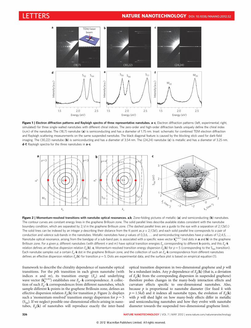
The results for three representative single-walled carbon nano-tubes are shown in Fig. 1. From the electron diffraction patternfor the first of these nanotubes (Fig. 1a) we determine its chiralindex to be (18,7), which means that this is a semiconducting nano-tube with a diameter of 1.75 nm. The second nanotube (Fig. 1b) hasa chiral index of (30,22), which means that it is also semiconducting(with a diameter of 3.54 nm). The third nanotube (Fig. 1c) has achiral index of (24,24), which means that it is metallic with a diam-eter of 3.25 nm. Each nanotube also exhibits distinct optical reson-ances in its Rayleigh spectrum (Fig. 1d–f). Our data complementprevious fluorescence studies of nanotubes with diameters in therange 0.6–1.3 nm (refs 17,18), and together they can be used as anatlas for determining the chiral index of a single-walled nanotubefrom a measurement of its optical resonances, and vice versa(Supplementary Section S4).
A number of techniques can be used to determine the chiralindex and optical resonances of single-walled nanotubes (hereafter
called nanotubes), but they are all limited in various ways.Fluorescence excitation spectroscopy, for example, allows the chiralindex to be determined from measurements of the fluorescence,but only for a small subset of semiconducting nanotubes17. Ramanspectroscopy is a more general technique, in principle, but it suffersfrom large uncertainties due to the presence of many overlappingresonant peaks from ensemble measurements19–21. The uncertaintyin our determination of the optical resonances for all nanotubes isless than 20 meV. This is significantly more accurate than previouscomprehensive optical assignments based on Raman mapping,where the difference between the measured and predicted opticaltransition energies is greater than 100 meV for many nanotubes21.
It should be noted that our results are based on suspended nano-tubes. It is known that environmental effects, such as the presence of asubstrate or surrounding micelles, can redshift the optical transition,predominantly due to dielectric screening. A comparison of nano-tubes suspended in air and nanotubes embedded in micelles showsthat this redshift is relatively constant at �20 meV for different nano-tubes18, and similar redshifts are expected for nanotubes deposited onsubstrates. Accordingly, a suitable correction should be made whencharacterizing nanotubes that are not suspended in air.
The relationship between the chiral index and the optical reson-ances of nanotubes reported here allows for a systematic examin-ation of excited-state properties in one-dimensional nanotubes.Although the optical transitions in nanotubes are excitonic innature, a convenient scheme by which to categorize the optical tran-sitions in an (n,m) nanotube is the zone-folding technique, in whichthe periodic boundary condition around the nanotube circumfer-ence leads to a quantization of wave vector (k), described by parallellines separated by 2/d in the graphene Brillouin zone5,6. In metallicnanotubes, one of the parallel k-lines passes through the K-point,which occurs when mod(n–m,3)¼ 0 (Fig. 2a). The other nanotubesare semiconducting with mod(n–m,3)¼ 1 or 2 (Fig. 2b). Each par-allel k-line describes one pair of conduction and valence sub-bandsin the nanotube. Transitions at the bandgaps of such sub-band pairslead to strong optical resonances, and these transitions are tradition-ally labelled Sii for semiconducting and Mii for metallic nanotubes,where i is the sub-band index. Equivalently, we can introduce aninteger p (¼ 1,2,3,4,5,6, . . .) to index optical transitions in bothsemiconducting and metallic nanotubes in the order of S11, S22,M11, S33, S44, M22, S55, S66, M33, S77, . . . (Table 1). Each nanotubeoptical transition can be associated with a specific wave vector kp
(n,m)
(for example, red dots in Fig. 2a,b) in the graphene Brillouin zonethat varies with nanotube chirality (n,m) and transition index p(for a detailed relation see Supplementary Section S2). The magni-tude of kp
(n,m) has a value of p × 2/(3d).The one-to-one mapping between a nanotube optical resonance
and a wave vector in the graphene Brillouin zone provides a
1Department of Physics, University of California at Berkeley, Berkeley, California 94720, USA, 2Institute of Physics, Chinese Academy of Sciences, Beijing100190, China, 3Materials Science Division, Lawrence Berkeley National Laboratory, Berkeley, California 94720, USA, 4School of Science, NorthwesternPolytechnic University, Xi’an 710072, China, 5Instituto de Fı́sica, Universidade Federal do Rio de Janeiro, Caixa Postal 68528, Rio de Janeiro, RJ 21941-972,Brazil, 6The Molecular Foundry, Lawrence Berkeley National Laboratory, Berkeley, California 94720, USA, 7International Center for Quantum Materials,School of Physics, Peking University, Beijing 100871, China. *e-mail: [email protected]; [email protected]
LETTERSPUBLISHED ONLINE: 15 APRIL 2012 | DOI: 10.1038/NNANO.2012.52
NATURE NANOTECHNOLOGY | VOL 7 | MAY 2012 | www.nature.com/naturenanotechnology 325
© 2012 Macmillan Publishers Limited. All rights reserved.
framework to describe the chirality dependence of nanotube opticaltransitions. For the pth transition in each given nanotube (withindices n and m), its transition energy (Ep) and underlyingwave vector (kp
(n,m)) establishes one Ep–k correspondence. A collec-tion of such Ep–k correspondences from different nanotubes, whichsample different k-points in the graphene Brillouin zone, defines aneffective dispersion relation Ep(k) for transition p. Figure 2c displayssuch a ‘momentum-resolved’ transition energy dispersion for p¼ 5(S44). If we neglect possible one-dimensional effects arising in nano-tubes, Ep(k) of nanotubes will reproduce exactly the inter-band
optical transition dispersion in two-dimensional graphene and p willbe a redundant index. Any p-dependence of Ep(k) (that is, a deviationof Ep(k) from the corresponding dispersion in suspended graphene)therefore probes changes in the many-body interaction effects andcurvature effects specific to one-dimensional nanotubes. Also,because p is proportional to nanotube diameter (for fixed k withp¼ 1.5kd) and it indexes all nanotube types, the evolution of Ep(k)with p will shed light on how many-body effects differ in metallicand semiconducting nanotubes and how they evolve with nanotubediameter towards the suspended two-dimensional graphene limit.
S 44 (e
V)
b c
K
ap = 3
3
2
12
0
−2 −20
2
p = 3
k y k y
S33M11 M11 S11S22
p = 4 p = 2p = 1
kxkx
K
ky (nm –1)
k x (nm
–1 )
Figure 2 | Momentum-resolved transitions with nanotube optical resonances. a,b, Zone-folding pictures of metallic (a) and semiconducting (b) nanotubes.
The contour curves are constant energy lines in the graphene Brillouin zone. The solid parallel lines describe available states consistent with the nanotube
boundary condition, which are separated by 2/d in the graphene Brillouin zone. (The dashed parallel lines are a guide to the eye with a separation of 2/(3d).)
The solid lines can be indexed by an integer p describing their distance from the K-point as p × 2/(3d), and each solid parallel line corresponds to a pair of
conduction and valence sub-bands in the nanotubes. Metallic nanotubes have p values of 0,3,6, . . . and semiconducting nanotubes have p values of 1,2,4,5, . . .
Nanotube optical resonance, arising from the bandgap of a sub-band pair, is associated with a specific wave vector kp(n,m ) (red dots in a and b) in the graphene
Brillouin zone. For a given p, different nanotubes (with different n and m) have optical transition energies Ep corresponding to different k-points, and this Ep–k
relation defines an effective dispersion relation Ep(k). c, Momentum-resolved transition energy dispersion Ep(k) for p¼ 5 (corresponding to the S44 transition).
Each nanotube samples out a certain Ep–k dot in the graphene Brillouin zone, and the collection of such an Ep–k correspondence from different nanotubes
defines an effective dispersion relation Ep(k) for transition p¼ 5. Dots are experimental data, and the surface plot is based on empirical equation (1).
(30,22) (24,24)
1.5 2.0 2.5 1.5 2.0 2.5 1.5 2.0 2.5
S33 S44S55 S66
S77
M22
M33
TEM/laserbeam
Energy (eV)Energy (eV) Energy (eV)
Inte
nsity
(a.u
.)
Inte
nsity
(a.u
.)
Inte
nsity
(a.u
.)
a
d e
b c
f
(18,7)
Figure 1 | Electron diffraction patterns and Rayleigh spectra of three representative nanotubes. a–c, Electron diffraction patterns (left, experimental; right,
simulated) for three single-walled nanotubes with different chiral indices. The zero-order and high-order diffraction bands uniquely define the chiral index
(n,m) of the nanotube. The (18,7) nanotube (a) is semiconducting and has a diameter of 1.75 nm. Inset: schematic for combined TEM electron diffraction
and Rayleigh scattering measurements on the same suspended nanotube. The black diagonal feature is caused by the blocking stick used for dark-field
imaging. The (30,22) nanotube (b) is semiconducting and has a diameter of 3.54 nm. The (24,24) nanotube (c) is metallic and has a diameter of 3.25 nm.
d–f, Rayleigh spectra for the three nanotubes in a–c.
LETTERS NATURE NANOTECHNOLOGY DOI: 10.1038/NNANO.2012.52
NATURE NANOTECHNOLOGY | VOL 7 | MAY 2012 | www.nature.com/naturenanotechnology326
© 2012 Macmillan Publishers Limited. All rights reserved.
To describe the effective dispersion such as that in Fig. 2c, weintroduce an empirical formula
Ep(k) = 2h− nF( p) × k + b× k2 + h( p) × k2 cos(3u) (1)
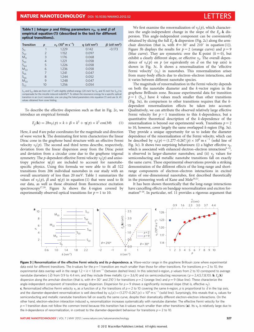
Here, k and u are polar coordinates for the magnitude and directionof wave vector k. The dominating first term characterizes the linearDirac cone in the graphene band structure with an effective Fermivelocity vF( p). The second and third terms describe, respectively,deviation from the linear dispersion away from the Dirac pointand deviation from a circular cone due to the graphene trigonalsymmetry. The p-dependent effective Fermi velocity vF( p) and aniso-tropy prefactor h( p) are included to account for nanotube-specific physics. Using this formula we were able to fit all 522transitions from 206 individual nanotubes in our study with anoverall uncertainty of less than 20 meV. Table 1 summarizes thevalues of vF( p), b and h( p) in equation (1) that were used to fitour data, as well as those obtained from fluorescence excitationspectroscopy17,18. Figure 3a shows the k-region covered byexperimentally observed optical transitions for p¼ 1 to 10.
We first examine the renormalization of vF( p), which character-izes the angle-independent change in the slope of the Ep–k dis-persion. This angle-independent component can be convenientlyobtained by slicing the full Ep–k dispersion (Fig. 2c) along the arm-chair direction (that is, with u¼ 308 and 2108 in equation (1)).Figure 3b displays the results for p¼ 2 (orange curve) and p¼ 9(blue curve). They are symmetric over the K-point (k¼ 0), butexhibit a clearly different slope, or effective vF. The overall depen-dence of vF( p) on p (or equivalently on d̄ on the top axis) isshown in Fig. 3c. It shows a renormalization of the ‘effectiveFermi velocity’ (vF) in nanotubes. This renormalization arisesfrom many-body effects due to electron–electron interactions, andit varies between different nanotube species.
The magnitude of renormalization in the Fermi velocity dependson both the nanotube diameter and the k-vector region in thegraphene Brillouin zone. Because experimental data for transitionp¼ 1 (S11) have k values much smaller than other transitions(Fig. 3a), its comparison to other transitions requires that the k-dependent renormalization effects be taken into account.Qualitatively, we can attribute the observed relatively large effectiveFermi velocity for p¼ 1 transitions to this k-dependence, but aquantitative theoretical description of the k-dependence of therenormalization is beyond our experimental work. Transitions p¼ 2to 10, however, cover largely the same overlapped k-region (Fig. 3a).They provide a unique opportunity for us to isolate the diameterdependence of the renormalization of the Fermi velocity, which canbe described by vF(p)¼ (1.277–0.267/p) × 106 m s21 (solid line ofFig. 3c). It shows two surprising behaviours: (i) a higher effective vF,which is associated with enhanced electron–electron interactions9–12,is observed in larger-diameter nanotubes; and (ii) vF values forsemiconducting and metallic nanotube transitions fall on exactlythe same curve. These experimental observations provide a strikingdemonstration of the different effects of the long-range and short-range components of electron–electron interactions in excitedstates of one-dimensional nanotubes, first described theoreticallyin the pioneering work of Kane and Mele10,11.
It has been shown theoretically that the long-range interactionshave cancelling effects on bandgap renormalization and exciton for-mation9–16. In particular, ref. 11 provides a rigorous argument that
Table 1 | Integer p and fitting parameters nF, h and b ofempirical equation (1) (described in the text for differentoptical transitions).
Transition p nF (106 m s21) h (eV nm2) b (eV nm2)
S11 1 1.229 0.142 –0.173S22 2 1.152 0.097M11 3 1.176 0.068S33 4 1.221 0.058S44 5 1.226 0.058M22 6 1.236 0.058S55 7 1.241 0.047S66 8 1.244 0.052M33 9 1.248 0.047S77 10 1.256 0.054
S11 and S22 data are from ref. 17 with slightly shifted energy (20 meV for S11 and 15 meV for S22) tocompensate for the micelle-induced redshifts18. To obtain the resonance energy for a specific opticaltransition in an (n,m) nanotube, one can plug the listed parameters into equation (1) and use (k, u)values obtained from zone folding.
−2 −1 00.0
0.5
1.0
1.5
2.0
2.5
θ = 210° θ = 30°
p = 2p = 9
1 2
E p(k
) (eV
)
b
0.6 1.0 1.4 1.8 2.2
2
4
6
8
10a
p
1 2 3 4 5 6 7 8 9 10
1.14
1.17
1.20
1.23
1.26
d (nm)
v F (10
6 m
s−1
)
p
0.9 1.6 2.3 3.0 3.7 4.4c
k (nm–1)k (nm–1)
M33
M22
S22
S33
S44
S55
S66
S77
M11
S11
Figure 3 | Renormalization of the effective Fermi velocity and its p-dependence. a, Wave-vector range in the graphene Brillouin zone where experimental
data exist for different transitions. The k-values for the p¼ 1 transition are much smaller than those for other transitions. For transitions p¼ 2 to 10, the
experimental data overlap well in the range 1.2 , k , 1.8 nm21 (between dashed lines). In this selected k-region, p values from 2 to 10 correspond to average
nanotube diameters (�d) from 0.9 to 4.4 nm, and they include three metallic (p¼ 3,6,9) and six semiconducting resonances (p¼ 2,4,5,7,8,10). b, Ep(k)
dispersion along the armchair direction (that is, with u¼ 308 and 2108) for transitions p¼ 2 (orange line) and p¼ 9 (blue line). These characterize the
angle-independent component of transition energy dispersion. Dispersion for p¼ 9 shows a significantly increased slope (that is, effective nF).
c, Renormalized effective Fermi velocity nF as a function of p. For transitions of p¼ 2 to 10 covering the same k-region, p is proportional to �d in the top axis,
and the diameter-dependent renormalization is well described by nF(p)¼ (1.277–0.267/p) × 106 m s21 (solid line). Surprisingly, this reveals that nF values for
semiconducting and metallic nanotube transitions fall on exactly the same curve, despite their dramatically different electron–electron interactions. On the
other hand, electron–electron interaction induced nF renormalization increases systematically with nanotube diameter. The effective Fermi velocity for the
p¼ 1 transition does not follow the common trend because this transition has k-values much smaller than other transitions (a). Its nF is relatively large due to
the k-dependence of renormalization, in contrast to the diameter-dependent behaviour for transitions p¼ 2 to 10.
NATURE NANOTECHNOLOGY DOI: 10.1038/NNANO.2012.52 LETTERS
NATURE NANOTECHNOLOGY | VOL 7 | MAY 2012 | www.nature.com/naturenanotechnology 327
© 2012 Macmillan Publishers Limited. All rights reserved.
the cancellation is perfect for a constant long-range interaction.Here, we demonstrate experimentally that such cancellation isalmost perfect for the actual long-range interaction in nanotubes:the semiconducting and metallic nanotubes have drastically differ-ent long-range electron–electron interactions, but their optical tran-sition energies fall perfectly on the same curve (Fig. 3c).
Short-range electron–electron interactions, however, show quali-tatively different behaviour: they produce a significant net blueshiftof optical transition energies9–11. Reference 11 shows theoreticallythat the effect of short-range interactions increases slightly but sys-tematically with nanotube diameter, in contrast to the commonnotion that many-body effects are always stronger in more one-dimensional structures. We demonstrate this diameter dependenceof short-range interaction experimentally in that vF( p) (that is,optical transition energy at the same k) increases with nanotubediameter. Interestingly, the effective Fermi velocity in large-diam-eter nanotubes should approach the ‘intrinsic’ vF in suspended gra-phene, and our measurements suggest a value of 1.28 × 10⁶ m s21.This is significantly larger than most reported Fermi velocity valuesfor supported graphene22,23, presumably due to reduced electron–electron interactions and Fermi velocity renormalization from sub-strate screening in supported samples.
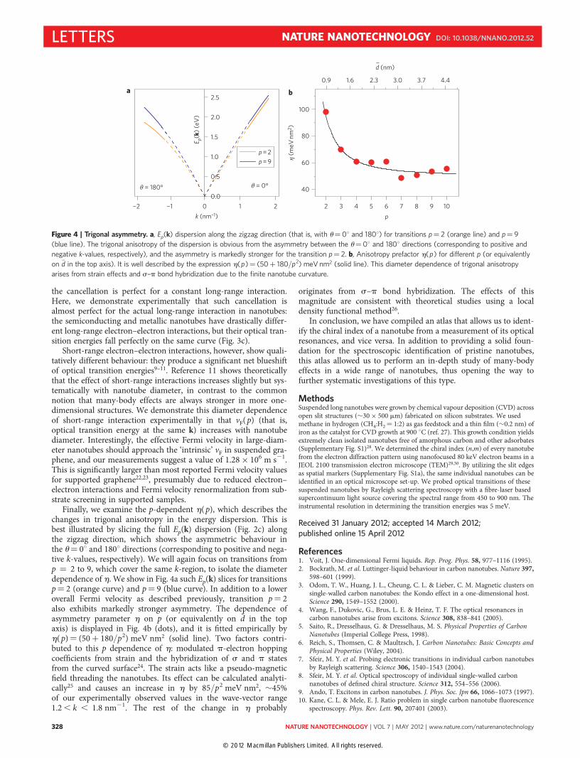
Finally, we examine the p-dependent h( p), which describes thechanges in trigonal anisotropy in the energy dispersion. This isbest illustrated by slicing the full Ep(k) dispersion (Fig. 2c) alongthe zigzag direction, which shows the asymmetric behaviour inthe u¼ 08 and 1808 directions (corresponding to positive and nega-tive k-values, respectively). We will again focus on transitions fromp ¼ 2 to 9, which cover the same k-region, to isolate the diameterdependence of h. We show in Fig. 4a such Ep(k) slices for transitionsp¼ 2 (orange curve) and p¼ 9 (blue curve). In addition to a loweroverall Fermi velocity as described previously, transition p¼ 2also exhibits markedly stronger asymmetry. The dependence ofasymmetry parameter h on p (or equivalently on d̄ in the topaxis) is displayed in Fig. 4b (dots), and it is fitted empirically byh( p)¼ (50þ 180/p2) meV nm2 (solid line). Two factors contri-buted to this p dependence of h: modulated p-electron hoppingcoefficients from strain and the hybridization of s and p statesfrom the curved surface24. The strain acts like a pseudo-magneticfield threading the nanotubes. Its effect can be calculated analyti-cally25 and causes an increase in h by 85/p2 meV nm2, �45%of our experimentally observed values in the wave-vector range1.2 , k , 1.8 nm21. The rest of the change in h probably
originates from s–p bond hybridization. The effects of thismagnitude are consistent with theoretical studies using a localdensity functional method26.
In conclusion, we have compiled an atlas that allows us to ident-ify the chiral index of a nanotube from a measurement of its opticalresonances, and vice versa. In addition to providing a solid foun-dation for the spectroscopic identification of pristine nanotubes,this atlas allowed us to perform an in-depth study of many-bodyeffects in a wide range of nanotubes, thus opening the way tofurther systematic investigations of this type.
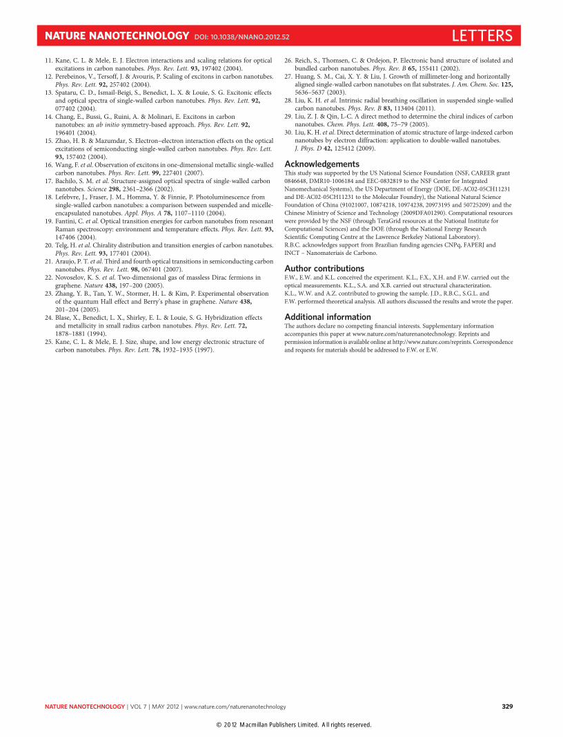
MethodsSuspended long nanotubes were grown by chemical vapour deposition (CVD) acrossopen slit structures (�30 × 500 mm) fabricated on silicon substrates. We usedmethane in hydrogen (CH4:H2¼ 1:2) as gas feedstock and a thin film (�0.2 nm) ofiron as the catalyst for CVD growth at 900 8C (ref. 27). This growth condition yieldsextremely clean isolated nanotubes free of amorphous carbon and other adsorbates(Supplementary Fig. S1)28. We determined the chiral index (n,m) of every nanotubefrom the electron diffraction pattern using nanofocused 80 keV electron beams in aJEOL 2100 transmission electron microscope (TEM)29,30. By utilizing the slit edgesas spatial markers (Supplementary Fig. S1a), the same individual nanotubes can beidentified in an optical microscope set-up. We probed optical transitions of thesesuspended nanotubes by Rayleigh scattering spectroscopy with a fibre-laser basedsupercontinuum light source covering the spectral range from 450 to 900 nm. Theinstrumental resolution in determining the transition energies was 5 meV.
Received 31 January 2012; accepted 14 March 2012;published online 15 April 2012
References1. Voit, J. One-dimensional Fermi liquids. Rep. Prog. Phys. 58, 977–1116 (1995).2. Bockrath, M. et al. Luttinger-liquid behaviour in carbon nanotubes. Nature 397,
598–601 (1999).3. Odom, T. W., Huang, J. L., Cheung, C. L. & Lieber, C. M. Magnetic clusters on
single-walled carbon nanotubes: the Kondo effect in a one-dimensional host.Science 290, 1549–1552 (2000).
4. Wang, F., Dukovic, G., Brus, L. E. & Heinz, T. F. The optical resonances incarbon nanotubes arise from excitons. Science 308, 838–841 (2005).
5. Saito, R., Dresselhaus, G. & Dresselhaus, M. S. Physical Properties of CarbonNanotubes (Imperial College Press, 1998).
6. Reich, S., Thomsen, C. & Maultzsch, J. Carbon Nanotubes: Basic Concepts andPhysical Properties (Wiley, 2004).
7. Sfeir, M. Y. et al. Probing electronic transitions in individual carbon nanotubesby Rayleigh scattering. Science 306, 1540–1543 (2004).
8. Sfeir, M. Y. et al. Optical spectroscopy of individual single-walled carbonnanotubes of defined chiral structure. Science 312, 554–556 (2006).
9. Ando, T. Excitons in carbon nanotubes. J. Phys. Soc. Jpn 66, 1066–1073 (1997).10. Kane, C. L. & Mele, E. J. Ratio problem in single carbon nanotube fluorescence
spectroscopy. Phys. Rev. Lett. 90, 207401 (2003).
2 3 4 5 6 7 8 9 10
40
60
80
100
b
η (m
eV nm
2 )
p
a
−2 −1 00.0
0.5
1.0
1.5
2.0
2.5
θ = 180° θ = 0°
p = 2p = 9
1 2
E p(k
) (eV
)
0.9 1.6 2.3 3.0 3.7 4.4
k (nm–1)
d (nm)−
Figure 4 | Trigonal asymmetry. a, Ep(k) dispersion along the zigzag direction (that is, with u¼08 and 1808) for transitions p¼ 2 (orange line) and p¼ 9
(blue line). The trigonal anisotropy of the dispersion is obvious from the asymmetry between the u¼08 and 1808 directions (corresponding to positive and
negative k-values, respectively), and the asymmetry is markedly stronger for the transition p¼ 2. b, Anisotropy prefactor h(p) for different p (or equivalently
on �d in the top axis). It is well described by the expression h(p)¼ (50þ 180/p2) meV nm2 (solid line). This diameter dependence of trigonal anisotropy
arises from strain effects and s–p bond hybridization due to the finite nanotube curvature.
LETTERS NATURE NANOTECHNOLOGY DOI: 10.1038/NNANO.2012.52
NATURE NANOTECHNOLOGY | VOL 7 | MAY 2012 | www.nature.com/naturenanotechnology328
© 2012 Macmillan Publishers Limited. All rights reserved.
11. Kane, C. L. & Mele, E. J. Electron interactions and scaling relations for opticalexcitations in carbon nanotubes. Phys. Rev. Lett. 93, 197402 (2004).
12. Perebeinos, V., Tersoff, J. & Avouris, P. Scaling of excitons in carbon nanotubes.Phys. Rev. Lett. 92, 257402 (2004).
13. Spataru, C. D., Ismail-Beigi, S., Benedict, L. X. & Louie, S. G. Excitonic effectsand optical spectra of single-walled carbon nanotubes. Phys. Rev. Lett. 92,077402 (2004).
14. Chang, E., Bussi, G., Ruini, A. & Molinari, E. Excitons in carbonnanotubes: an ab initio symmetry-based approach. Phys. Rev. Lett. 92,196401 (2004).
15. Zhao, H. B. & Mazumdar, S. Electron–electron interaction effects on the opticalexcitations of semiconducting single-walled carbon nanotubes. Phys. Rev. Lett.93, 157402 (2004).
16. Wang, F. et al. Observation of excitons in one-dimensional metallic single-walledcarbon nanotubes. Phys. Rev. Lett. 99, 227401 (2007).
17. Bachilo, S. M. et al. Structure-assigned optical spectra of single-walled carbonnanotubes. Science 298, 2361–2366 (2002).
18. Lefebvre, J., Fraser, J. M., Homma, Y. & Finnie, P. Photoluminescence fromsingle-walled carbon nanotubes: a comparison between suspended and micelle-encapsulated nanotubes. Appl. Phys. A 78, 1107–1110 (2004).
19. Fantini, C. et al. Optical transition energies for carbon nanotubes from resonantRaman spectroscopy: environment and temperature effects. Phys. Rev. Lett. 93,147406 (2004).
20. Telg, H. et al. Chirality distribution and transition energies of carbon nanotubes.Phys. Rev. Lett. 93, 177401 (2004).
21. Araujo, P. T. et al. Third and fourth optical transitions in semiconducting carbonnanotubes. Phys. Rev. Lett. 98, 067401 (2007).
22. Novoselov, K. S. et al. Two-dimensional gas of massless Dirac fermions ingraphene. Nature 438, 197–200 (2005).
23. Zhang, Y. B., Tan, Y. W., Stormer, H. L. & Kim, P. Experimental observationof the quantum Hall effect and Berry’s phase in graphene. Nature 438,201–204 (2005).
24. Blase, X., Benedict, L. X., Shirley, E. L. & Louie, S. G. Hybridization effectsand metallicity in small radius carbon nanotubes. Phys. Rev. Lett. 72,1878–1881 (1994).
25. Kane, C. L. & Mele, E. J. Size, shape, and low energy electronic structure ofcarbon nanotubes. Phys. Rev. Lett. 78, 1932–1935 (1997).
26. Reich, S., Thomsen, C. & Ordejon, P. Electronic band structure of isolated andbundled carbon nanotubes. Phys. Rev. B 65, 155411 (2002).
27. Huang, S. M., Cai, X. Y. & Liu, J. Growth of millimeter-long and horizontallyaligned single-walled carbon nanotubes on flat substrates. J. Am. Chem. Soc. 125,5636–5637 (2003).
28. Liu, K. H. et al. Intrinsic radial breathing oscillation in suspended single-walledcarbon nanotubes. Phys. Rev. B 83, 113404 (2011).
29. Liu, Z. J. & Qin, L-C. A direct method to determine the chiral indices of carbonnanotubes. Chem. Phys. Lett. 408, 75–79 (2005).
30. Liu, K. H. et al. Direct determination of atomic structure of large-indexed carbonnanotubes by electron diffraction: application to double-walled nanotubes.J. Phys. D 42, 125412 (2009).
AcknowledgementsThis study was supported by the US National Science Foundation (NSF, CAREER grant0846648, DMR10-1006184 and EEC-0832819 to the NSF Center for IntegratedNanomechanical Systems), the US Department of Energy (DOE, DE-AC02-05CH11231and DE-AC02-05CH11231 to the Molecular Foundry), the National Natural ScienceFoundation of China (91021007, 10874218, 10974238, 20973195 and 50725209) and theChinese Ministry of Science and Technology (2009DFA01290). Computational resourceswere provided by the NSF (through TeraGrid resources at the National Institute forComputational Sciences) and the DOE (through the National Energy ResearchScientific Computing Centre at the Lawrence Berkeley National Laboratory).R.B.C. acknowledges support from Brazilian funding agencies CNPq, FAPERJ andINCT – Nanomateriais de Carbono.
Author contributionsF.W., E.W. and K.L. conceived the experiment. K.L., F.X., X.H. and F.W. carried out theoptical measurements. K.L., S.A. and X.B. carried out structural characterization.K.L., W.W. and A.Z. contributed to growing the sample. J.D., R.B.C., S.G.L. andF.W. performed theoretical analysis. All authors discussed the results and wrote the paper.
Additional informationThe authors declare no competing financial interests. Supplementary informationaccompanies this paper at www.nature.com/naturenanotechnology. Reprints andpermission information is available online at http://www.nature.com/reprints. Correspondenceand requests for materials should be addressed to F.W. or E.W.
NATURE NANOTECHNOLOGY DOI: 10.1038/NNANO.2012.52 LETTERS
NATURE NANOTECHNOLOGY | VOL 7 | MAY 2012 | www.nature.com/naturenanotechnology 329
© 2012 Macmillan Publishers Limited. All rights reserved.

SUPPLEMENTARY INFORMATIONDOI: 10.1038/NNANO.2012.52
NATURE NANOTECHNOLOGY | www.nature.com/naturenanotechnology 1
Supplementary Information for
An Atlas of Carbon Nanotube Optical Transitions
Kaihui Liu, Jack Deslippe, Fajun Xiao, Rodrigo B. Capaz, Xiaoping Hong, Shaul Aloni,
Alex Zettl, Wenlong Wang, Xuedong Bai, Steven G. Louie, Enge Wang, Feng Wang
© 2012 Macmillan Publishers Limited. All rights reserved.
2 NATURE NANOTECHNOLOGY | www.nature.com/naturenanotechnology
SUPPLEMENTARY INFORMATION DOI: 10.1038/NNANO.2012.52
1. Isolated single-wall carbon nanotubes suspended on the open slit
10 nm
slit
a
b
100 µm
Figure S1. (a) Scanning electron microscope image of suspended nanotubes. The
nanotubes are controlled to be well separated from each other with an average separation
over 30 μm. By utilizing the slit edges as the spatial markers, we can reliably locate any
given nanotube in both transmission electron microscope and optical microscopy setup.
(b) High-resolution transmission electron micrograph of a nanotube. It is seen to be
single-wall character with clean surface.
2. The wavevector k (n,m)ii corresponding to the bandgap of the ith sub-band pair in
an (n,m) nanotube
The ith optical resonance in an (n,m) nanotube arises from the electronic transition at
the bandgap of ith sub-band pair in the nanotube, and it corresponds to a unique
wavevector k . The wavevector k can be described in the polar coordinate by (k,
θ). The magnitude k depends on nanotube diameter (d) and ith transition, and it has a
(n,m)ii
(n,m)ii
value of p×2/(3d) for all nanotube species. The relation between integers p and i is listed
in Table S1. The polar angle θ is related to the nanotube chiral angle
-1α=tan ( 3m/(2n+m)) in the following way.
Semiconducting nanotubes:
θ for ith transition in semiconducting nanotubes with mod(n-m,3)=1. =α+i*π
for ith transition in semiconducting nanotubes with mod(n-m,3)=2. θ=α+(i+1)*π
Metallic nanotubes (mod(n-m, 3)=0): Two sub-bands exist for ith transition.
θ for the higher energy sub-band. =α
θ for the lower energy sub-band. =α+π
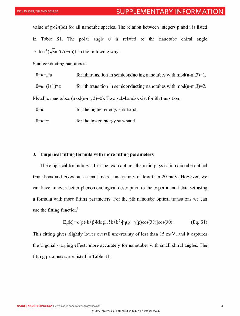
3. Empirical fitting formula with more fitting parameters
The empirical formula Eq. 1 in the text captures the main physics in nanotube optical
transitions and gives out a small overal uncertainty of less than 20 meV. However, we
can have an even better phenomenological description to the experimental data set using
a formula with more fitting parameters. For the pth nanotube optical transitions we can
use the fitting function1
Ep(k) (Eq. S1) 2=α(p) k+β klog1.5k+k [η(p)+γ(p)cos(3θ)]cos(3θ).i i i
This fitting gives slightly lower overall uncertainty of less than 15 meV, and it captures
the trigonal warping effects more accurately for nanotubes with small chiral angles. The
fitting parameters are listed in Table S1.
© 2012 Macmillan Publishers Limited. All rights reserved.
NATURE NANOTECHNOLOGY | www.nature.com/naturenanotechnology 3
SUPPLEMENTARY INFORMATIONDOI: 10.1038/NNANO.2012.52
1. Isolated single-wall carbon nanotubes suspended on the open slit
10 nm
slit
a
b
100 µm
Figure S1. (a) Scanning electron microscope image of suspended nanotubes. The
nanotubes are controlled to be well separated from each other with an average separation
over 30 μm. By utilizing the slit edges as the spatial markers, we can reliably locate any
given nanotube in both transmission electron microscope and optical microscopy setup.
(b) High-resolution transmission electron micrograph of a nanotube. It is seen to be
single-wall character with clean surface.
2. The wavevector k (n,m)ii corresponding to the bandgap of the ith sub-band pair in
an (n,m) nanotube
The ith optical resonance in an (n,m) nanotube arises from the electronic transition at
the bandgap of ith sub-band pair in the nanotube, and it corresponds to a unique
wavevector k . The wavevector k can be described in the polar coordinate by (k,
θ). The magnitude k depends on nanotube diameter (d) and ith transition, and it has a
(n,m)ii
(n,m)ii
value of p×2/(3d) for all nanotube species. The relation between integers p and i is listed
in Table S1. The polar angle θ is related to the nanotube chiral angle
-1α=tan ( 3m/(2n+m)) in the following way.
Semiconducting nanotubes:
θ for ith transition in semiconducting nanotubes with mod(n-m,3)=1. =α+i*π
for ith transition in semiconducting nanotubes with mod(n-m,3)=2. θ=α+(i+1)*π
Metallic nanotubes (mod(n-m, 3)=0): Two sub-bands exist for ith transition.
θ for the higher energy sub-band. =α
θ for the lower energy sub-band. =α+π
3. Empirical fitting formula with more fitting parameters
The empirical formula Eq. 1 in the text captures the main physics in nanotube optical
transitions and gives out a small overal uncertainty of less than 20 meV. However, we
can have an even better phenomenological description to the experimental data set using
a formula with more fitting parameters. For the pth nanotube optical transitions we can
use the fitting function1
Ep(k) (Eq. S1) 2=α(p) k+β klog1.5k+k [η(p)+γ(p)cos(3θ)]cos(3θ).i i i
This fitting gives slightly lower overall uncertainty of less than 15 meV, and it captures
the trigonal warping effects more accurately for nanotubes with small chiral angles. The
fitting parameters are listed in Table S1.
© 2012 Macmillan Publishers Limited. All rights reserved.
4 NATURE NANOTECHNOLOGY | www.nature.com/naturenanotechnology
SUPPLEMENTARY INFORMATION DOI: 10.1038/NNANO.2012.52
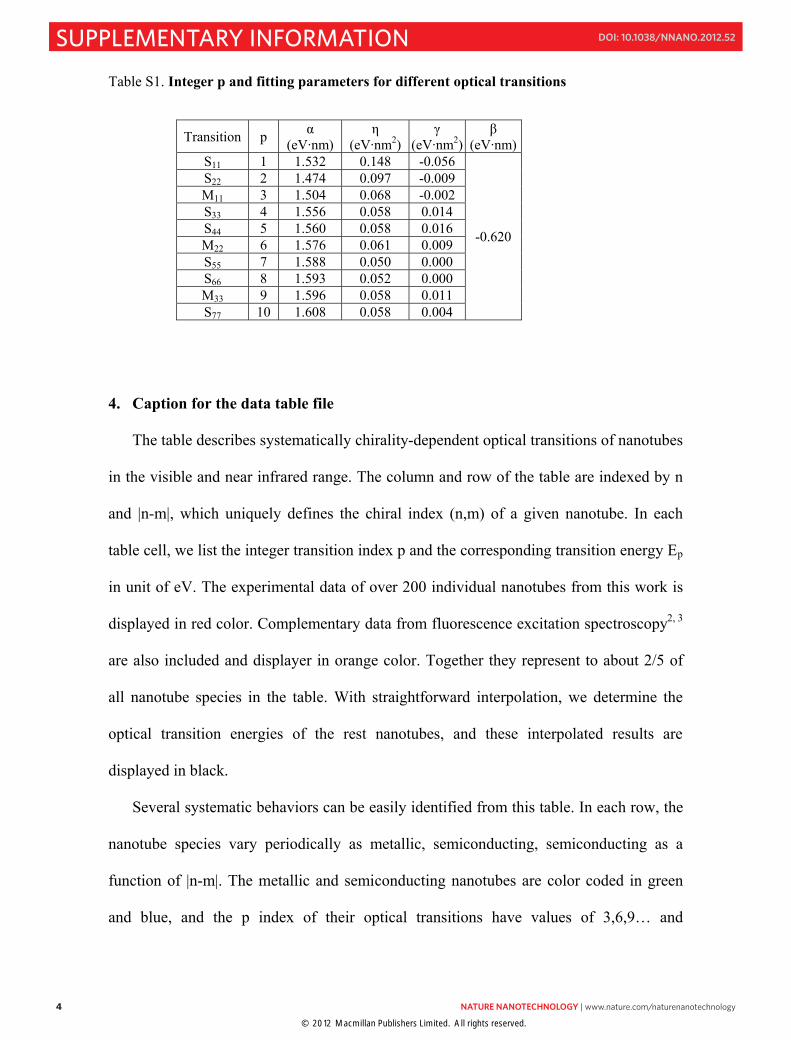
Table S1. Integer p and fitting parameters for different optical transitions
Transition p α (eV·nm)
η (eV·nm2)
γ (eV·nm2)
β (eV·nm)
S11 1 1.532 0.148 -0.056
-0.620
S22 2 1.474 0.097 -0.009M11 3 1.504 0.068 -0.002S33 4 1.556 0.058 0.014 S44 5 1.560 0.058 0.016 M22 6 1.576 0.061 0.009 S55 7 1.588 0.050 0.000 S66 8 1.593 0.052 0.000 M33 9 1.596 0.058 0.011 S77 10 1.608 0.058 0.004
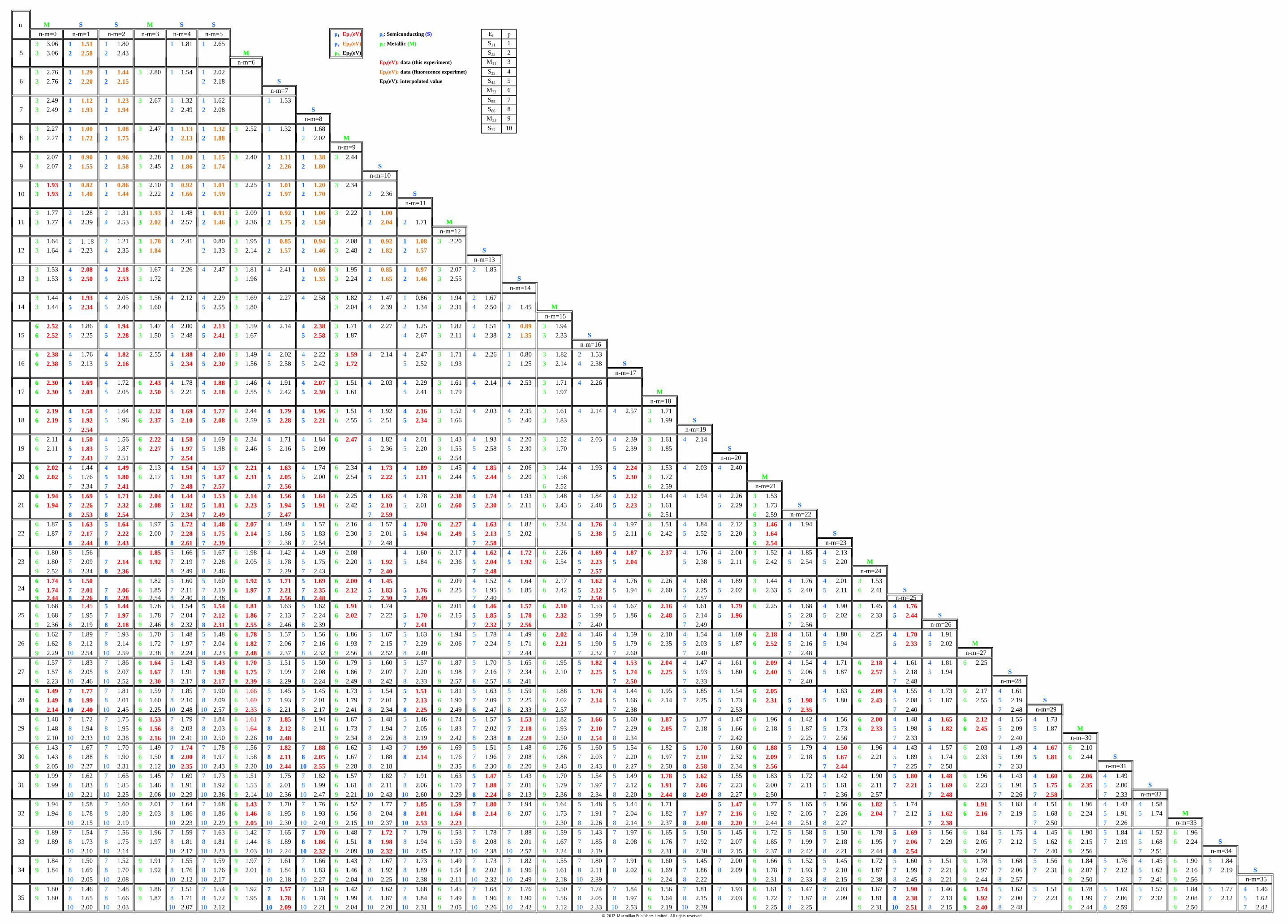
4. Caption for the data table file
The table describes systematically chirality-dependent optical transitions of nanotubes
in the visible and near infrared range. The column and row of the table are indexed by n
and |n-m|, which uniquely defines the chiral index (n,m) of a given nanotube. In each
table cell, we list the integer transition index p and the corresponding transition energy Ep
in unit of eV. The experimental data of over 200 individual nanotubes from this work is
displayed in red color. Complementary data from fluorescence excitation spectroscopy2, 3
are also included and displayer in orange color. Together they represent to about 2/5 of
all nanotube species in the table. With straightforward interpolation, we determine the
optical transition energies of the rest nanotubes, and these interpolated results are
displayed in black.
Several systematic behaviors can be easily identified from this table. In each row, the
nanotube species vary periodically as metallic, semiconducting, semiconducting as a
function of |n-m|. The metallic and semiconducting nanotubes are color coded in green
and blue, and the p index of their optical transitions have values of 3,6,9… and
1,2,4,5,7…, respectively. In each column, the diameter of the nanotube becomes larger
with the column index n, and the corresponding transition index p increases
monotonically for transitions in the same energy range. More detailed analysis and
understanding of the table is described in the text.
© 2012 Macmillan Publishers Limited. All rights reserved.

NATURE NANOTECHNOLOGY | www.nature.com/naturenanotechnology 5
SUPPLEMENTARY INFORMATIONDOI: 10.1038/NNANO.2012.52
Table S1. Integer p and fitting parameters for different optical transitions
Transition p α (eV·nm)
η (eV·nm2)
γ (eV·nm2)
β (eV·nm)
S11 1 1.532 0.148 -0.056
-0.620
S22 2 1.474 0.097 -0.009M11 3 1.504 0.068 -0.002S33 4 1.556 0.058 0.014 S44 5 1.560 0.058 0.016 M22 6 1.576 0.061 0.009 S55 7 1.588 0.050 0.000 S66 8 1.593 0.052 0.000 M33 9 1.596 0.058 0.011 S77 10 1.608 0.058 0.004
4. Caption for the data table file
The table describes systematically chirality-dependent optical transitions of nanotubes
in the visible and near infrared range. The column and row of the table are indexed by n
and |n-m|, which uniquely defines the chiral index (n,m) of a given nanotube. In each
table cell, we list the integer transition index p and the corresponding transition energy Ep
in unit of eV. The experimental data of over 200 individual nanotubes from this work is
displayed in red color. Complementary data from fluorescence excitation spectroscopy2, 3
are also included and displayer in orange color. Together they represent to about 2/5 of
all nanotube species in the table. With straightforward interpolation, we determine the
optical transition energies of the rest nanotubes, and these interpolated results are
displayed in black.
Several systematic behaviors can be easily identified from this table. In each row, the
nanotube species vary periodically as metallic, semiconducting, semiconducting as a
function of |n-m|. The metallic and semiconducting nanotubes are color coded in green
and blue, and the p index of their optical transitions have values of 3,6,9… and
1,2,4,5,7…, respectively. In each column, the diameter of the nanotube becomes larger
with the column index n, and the corresponding transition index p increases
monotonically for transitions in the same energy range. More detailed analysis and
understanding of the table is described in the text.
© 2012 Macmillan Publishers Limited. All rights reserved.
6 NATURE NANOTECHNOLOGY | www.nature.com/naturenanotechnology
SUPPLEMENTARY INFORMATION DOI: 10.1038/NNANO.2012.52
References:
1 Kane, C. L. & Mele, E. J. Electron interactions and scaling relations for optical excitations in
carbon nanotubes. Phys. Rev. Lett. 93, 197402 (2004).
2 Bachilo, S. M. et al. Structure-assigned optical spectra of single-walled carbon nanotubes.
Science 298, 2361-2366 (2002).
3 Lefebvre, J., Fraser, J. M., Homma, Y. & Finnie, P. Photoluminescence from single-walled
carbon nanotubes: a comparison between suspended and micelle-encapsulated nanotubes.
Appl. Phys. a-Mater. 78, 1107-1110 (2004).
© 2012 Macmillan Publishers Limited. All rights reserved.
M 36
2 1.72 2 1.75 2 2.13 2 1.88
3 4 4 3 4 2 3 2 2 2 2 M11
6 2.30 4 1.69 4 1.72 6 2.43 4 1.78 4 1.88 3 1.46 4 1.91 4 2.07 3 1.51 4 2.03 4 2.29 3 1.61 4 2.14 4 2.53 3 1.71 4 2.26
6 4 4 6 4 4 6 4 4 6 4 4 3 4 4 3 4 4 3 4 4
m9 10 10 9 10 10 9 8 8 9 8 8 9 8 8 9 7 7 7 7 7
10 10 9 10 10 9 10 10 9 10 10 9 8 9 8 8 8 9 9
10 2.00 10 2.03 10 2.07 10 2.12 10 2.09 10 2.21 9 2.04 10 2.20 10 2.31 9 2.05 10 2.26 10 2.42 9 2.12 10 2.33 10 2.53 9 2.19 10 2.39 9 2.25 8 2.25 9 2.31 10 2.51 8 2.15 9 2.40 8 2.48 9 2.44 8 2.59 9 2.50 7 2.42
n M S S M S S n-m=0 n-m=1 n-m=2 n-m=3 n-m=4 n-m=5 p1 Ep1(eV) pi: Semiconducting (S) Eii p
53 3.06 1 1.51 1 1.80 1 1.81 1 2.65 p2 Ep2(eV) pi: Metallic (M) S11 1 3 3.06 2 2.58 2 2.43 M p3 Ep3(eV) S22 2 6n-m= Epi M(eV): data (this experiment) 11 3
63 2.76 1 1.29 1 1.44 3 2.80 1 1.54 1 2.02 Epi(eV): data (fluorecence experimet) S33 4 3 2.76 2 2.20 2 2.15 2 2.18 S Epi(eV): interpolated value S44 5 n-m=7 M22 6
73 2.49 1 1.12 1 1.23 3 2.67 1 1.32 1 1.62 1 1.53 S55 7 3 2.49 2 1.93 2 1.94 2 2.49 2 2.08 S S66 8 n-m=8 M33 9
83 2.27 1 1.00 1 1.08 3 2.47 1 1.13 1 1.32 3 2.52 1 1.32 1 1.68 S77 10 3 2.27 2 1.72 2 1.75 2 2.13 2 1.88 2 2.02 M n-m=9
93 2.07 1 0.90 1 0.96 3 2.28 1 1.00 1 1.15 3 2.40 1 1.11 1 1.38 3 2.44 3 2.07 2 1.55 2 1.58 3 2.45 2 1.86 2 1.74 2 2.26 2 1.80 S n-m=10
103 1.93 1 0.82 1 0.86 3 2.10 1 0.92 1 1.01 3 2.25 1 1.01 1 1.20 3 2.34 3 1.93 2 1.40 2 1.44 3 2.22 2 1.66 2 1.59 2 1.97 2 1.70 2 2.36 S n-m=11
113 1.77 2 1.28 2 1.31 3 1.93 2 1.48 1 0.91 3 2.09 1 0.92 1 1.06 3 2.22 1 1.00 3 1 771.77 4 2 392.39 4 2 532.53 3 2 022.02 4 2 572.57 2 1 461.46 3 2 362.36 2 1 751.75 2 1 581.58 2 2 042.04 2 1 711.71 M n-m=12
123 1.64 2 1.18 2 1.21 3 1.78 4 2.41 1 0.80 3 1.95 1 0.85 1 0.94 3 2.08 1 0.92 1 1.08 3 2.20 3 1.64 4 2.23 4 2.35 3 1.84 2 1.33 3 2.14 2 1.57 2 1.46 3 2.48 2 1.82 2 1.57 S n-m=13
133 1.53 4 2.08 4 2.18 3 1.67 4 2.26 4 2.47 3 1.81 4 2.41 1 0.86 3 1.95 1 0.85 1 0.97 3 2.07 2 1.85 3 1.53 5 2.50 5 2.53 3 1.72 3 1.96 2 1.35 3 2.24 2 1.65 2 1.46 3 2.55 S n-m=14
143 1.44 4 1.93 4 2.05 3 1.56 4 2.12 4 2.29 3 1.69 4 2.27 4 2.58 3 1.82 2 1.47 1 0.86 3 1.94 2 1.67 3 1.44 5 2.34 5 2.40 3 1.60 5 2.55 3 1.80 3 2.04 4 2.39 2 1.34 3 2.31 4 2.50 2 1.45 M n-m=15
156 2.52 4 1.86 4 1.94 3 1.47 4 2.00 4 2.13 3 1.59 4 2.14 4 2.38 3 1.71 4 2.27 2 1.25 3 1.82 2 1.51 1 0.89 3 1.94
S6
2.52
5
2.25
5
2.28
3
1.50
5
2.48
5
2.41
3
1.67
5
2.58
3
1.87
4
2.67
3
2.11
4
2.38
2
1.35
3
2.33 n-m=16
166 2.38 4 1.76 4 1.82 6 2.55 4 1.88 4 2.00 3 1.49 4 2.02 4 2.22 3 1.59 4 2.14 4 2.47 3 1.71 4 2.26 1 0.80 3 1.82 2 1.53 6 2.38 5 2.13 5 2.16 5 2.34 5 2.30 3 1.56 5 2.58 5 2.42 3 1.72 5 2.52 3 1.93 2 1.25 3 2.14 4 2.38 S
17
n-m=17 6 2.30 4 1.69 4 1.72 6 2.43 4 1.78 4 1.88 3 1.46 4 1.91 4 2.07 3 1.51 4 2.03 4 2.29 3 1.61 4 2.14 4 2.53 3 1.71 4 2.26 6 2.30 5 2.03 5 2.05 6 2.50 5 2.21 5 2.18 6 2.55 5 2.42 5 2.30 3 1.61 5 2.41 3 1.79 3 1.97 M
18
n-m=18 6 2.19 4 1.58 4 1.64 6 2.32 4 1.69 4 1.77 6 2.44 4 1.79 4 1.96 3 1.51 4 1.92 4 2.16 3 1.52 4 2.03 4 2.35 3 1.61 4 2.14 4 2.57 3 1.71 6 2.19 5 1.92 5 1.96 6 2.37 5 2.10 5 2.08 6 2.59 5 2.28 5 2.21 6 2.55 5 2.51 5 2.34 3 1.66 5 2.40 3 1.83 3 1.99 S
19
7 2.54 n-m=19 6 2.11 4 1.50 4 1.56 6 2.22 4 1.58 4 1.69 6 2.34 4 1.71 4 1.84 6 2.47 4 1.82 4 2.01 3 1.43 4 1.93 4 2.20 3 1.52 4 2.03 4 2.39 3 1.61 4 2.14 6 2.11 5 1.83 5 1.87 6 2.27 5 1.97 5 1.98 6 2.46 5 2.16 5 2.09 5 2.36 5 2.20 3 1.55 5 2.58 5 2.30 3 1.70 5 2.39 3 1.85 S
20
7 2.43 7 2.51 7 2.54 6 2.54 n-m=20 6 2 022.02 4 1 441.44 4 1 491.49 6 2 132.13 4 1 541.54 4 1 571.57 6 2 212.21 4 1 631.63 4 1 741.74 6 2 342.34 4 1 731.73 4 1 891.89 3 1 451.45 4 1 851.85 4 2 062.06 3 1 441.44 4 1 931.93 4 2 242.24 3 1 531.53 4 2 032.03 4 2 402.40 6 2.02 5 1.76 5 1.80 6 2.17 5 1.91 5 1.87 6 2.31 5 2.05 5 2.00 6 2.54 5 2.22 5 2.11 6 2.44 5 2.44 5 2.20 3 1.58 5 2.30 3 1.72 M
21
7 2.34 7 2.41 7 2.48 7 2.57 7 2.56 6 2.52 6 2.59 n-m=21 6 1.94 5 1.69 5 1.71 6 2.04 4 1.44 4 1.53 6 2.14 4 1.56 4 1.64 6 2.25 4 1.65 4 1.78 6 2.38 4 1.74 4 1.93 3 1.48 4 1.84 4 2.12 3 1.44 4 1.94 4 2.26 3 1.53 6 1.94 7 2.26 7 2.32 6 2.08 5 1.82 5 1.81 6 2.23 5 1.94 5 1.91 6 2.42 5 2.10 5 2.01 6 2.60 5 2.30 5 2.11 6 2.43 5 2.48 5 2.23 3 1.61 5 2.29 3 1.73 S
22
8 2.53 8 2.54 7 2.34 7 2.49 7 2.47 7 2.59 6 2.51 6 2.59 n-m=22 6 1.87 5 1.63 5 1.64 6 1.97 5 1.72 4 1.48 6 2.07 4 1.49 4 1.57 6 2.16 4 1.57 4 1.70 6 2.27 4 1.63 4 1.82 6 2.34 4 1.76 4 1.97 3 1.51 4 1.84 4 2.12 3 1.46 4 1.94 6 1.87 7 2.17 7 2.22 6 2.00 7 2.28 5 1.75 6 2.14 5 1.86 5 1.83 6 2.30 5 2.01 5 1.94 6 2.49 5 2.13 5 2.02 5 2.38 5 2.11 6 2.42 5 2.52 5 2.20 3 1.64 S
23
8 2.44 8 2.43 8 2.61 7 2.39 7 2.38 7 2.54 7 2.48 7 2.58 6 2.54 n-m=23 6 1.80 5 1.56 6 1.85 5 1.66 5 1.67 6 1.98 4 1.42 4 1.49 6 2.08 4 1.60 6 2.17 4 1.62 4 1.72 6 2.26 4 1.69 4 1.87 6 2.37 4 1.76 4 2.00 3 1.52 4 1.85 4 2.13 6 1.80 7 2.09 7 2.14 6 1.92 7 2.19 7 2.28 6 2.05 5 1.78 5 1.75 6 2.20 5 1.92 5 1.84 6 2.36 5 2.04 5 1.92 6 2.54 5 2.23 5 2.04 5 2.38 5 2.11 6 2.42 5 2.54 5 2.20 M
24
9 2.52 8 2.34 8 2.36 8 2.49 8 2.46 7 2.29 7 2.43 7 2.40 7 2.48 7 2.57 n-m=24 6 1.74 5 1.50 6 1.82 5 1.60 5 1.60 6 1.92 5 1.71 5 1.69 6 2.00 4 1.45 6 2.09 4 1.52 4 1.64 6 2.17 4 1.62 4 1.76 6 2.26 4 1.68 4 1.89 3 1.44 4 1.76 4 2.01 3 1.53 6 1.74 7 2.01 7 2.06 6 1.85 7 2.11 7 2.19 6 1.97 7 2.21 7 2.35 6 2.12 5 1.83 5 1.76 6 2.25 5 1.95 5 1.85 6 2.42 5 2.12 5 1.94 6 2.60 5 2.25 5 2.02 6 2.33 5 2.40 5 2.11 6 2.41 S
25
9 2.44 8 2.26 8 2.28 9 2.54 8 2.40 8 2.38 8 2.56 8 2.48 7 2.30 7 2.49 7 2.40 7 2.50 7 2.57 n-m=25 6 1.68 5 1.45 5 1.44 6 1.76 5 1.54 5 1.54 6 1.81 5 1.63 5 1.62 6 1.91 5 1.74 6 2.01 4 1.46 4 1.57 6 2.10 4 1.53 4 1.67 6 2.16 4 1.61 4 1.79 6 2.25 4 1.68 4 1.90 3 1.45 4 1.76 6 1.68 7 1.95 7 1.97 6 1.78 7 2.04 7 2.12 6 1.86 7 2.13 7 2.24 6 2.02 7 2.22 5 1.70 6 2.15 5 1.85 5 1.78 6 2.32 5 1.99 5 1.86 6 2.48 5 2.14 5 1.96 5 2.28 5 2.02 6 2.33 5 2.44 S
26
9 2.36 8 2.19 8 2.18 9 2.46 8 2.32 8 2.31 9 2.55 8 2.46 8 2.39 7 2.41 7 2.32 7 2.56 7 2.40 7 2.49 7 2.56 n-m=26 6 1.62 7 1.89 7 1.93 6 1.70 5 1.48 5 1.48 6 1.78 5 1.57 5 1.56 6 1.86 5 1.67 5 1.63 6 1.94 5 1.78 4 1.49 6 2.02 4 1.46 4 1.59 6 2.10 4 1.54 4 1.69 6 2.18 4 1.61 4 1.80 6 2.25 4 1.70 4 1.91 6 1.62 8 2.12 8 2.14 6 1.72 7 1.97 7 2.04 6 1.82 7 2.06 7 2.16 6 1.93 7 2.15 7 2.29 6 2.06 7 2.24 5 1.71 6 2.21 5 1.90 5 1.79 6 2.35 5 2.03 5 1.87 6 2.52 5 2.16 5 1.94 5 2.33 5 2.02 M
27
9 2.29 10 2.54 10 2.59 9 2.38 8 2.24 8 2.23 9 2.48 8 2.37 8 2.32 9 2.56 8 2.52 8 2.40 7 2.44 7 2.32 7 2.60 7 2.40 7 2.48 n-m=27 6 1.57 7 1.83 7 1.86 6 1.64 5 1.43 5 1.43 6 1.70 5 1.51 5 1.50 6 1.79 5 1.60 5 1.57 6 1.87 5 1.70 5 1.65 6 1.95 5 1.82 4 1.53 6 2.04 4 1.47 4 1.61 6 2.09 4 1.54 4 1.71 6 2.18 4 1.61 4 1.81 6 2.25 6 1.57 8 2.05 8 2.07 6 1.67 7 1.91 7 1.98 6 1.75 7 1.99 7 2.08 6 1.86 7 2.07 7 2.20 6 1.98 7 2.16 7 2.34 6 2.10 7 2.25 5 1.74 6 2.25 5 1.93 5 1.80 6 2.40 5 2.06 5 1.87 6 2.57 5 2.18 5 1.94 S
28
9 2.23 10 2.46 10 2.52 9 2.30 8 2.17 8 2.17 9 2.39 8 2.29 8 2.24 9 2.49 8 2.42 8 2.33 9 2.57 8 2.57 8 2.41 7 2.50 7 2.33 7 2.40 7 2.48 n-m=28 6 1.49 7 1.77 7 1.81 6 1.59 7 1.85 7 1.90 6 1.66 5 1.45 5 1.45 6 1.73 5 1.54 5 1.51 6 1.81 5 1.63 5 1.59 6 1.88 5 1.76 4 1.44 6 1.95 5 1.85 4 1.54 6 2.05 4 1.63 6 2.09 4 1.55 4 1.73 6 2.17 4 1.61 6 1.49 8 1.99 8 2.01 6 1.60 8 2.10 8 2.09 6 1.69 7 1.93 7 2.01 6 1.79 7 2.01 7 2.13 6 1.90 7 2.09 7 2.25 6 2.02 7 2.14 5 1.66 6 2.14 7 2.25 5 1.73 6 2.31 5 1.98 5 1.80 6 2.43 5 2.08 5 1.87 6 2.55 5 2.19 S
29
9 2 142.14 10 2 402.40 10 2 452.45 9 2 252.25 10 2 482.48 10 2 572.57 9 2 332.33 8 2 212.21 8 2 172.17 9 2 412.41 8 2 342.34 8 2 252.25 9 2 492.49 8 2 472.47 8 2 332.33 9 2 572.57 7 2 382.38 7 2 532.53 7 2 352.35 7 2 402.40 7 2 482.48 n- =29n-m=29 6 1.48 7 1.72 7 1.75 6 1.53 7 1.79 7 1.84 6 1.61 7 1.85 7 1.94 6 1.67 5 1.48 5 1.46 6 1.74 5 1.57 5 1.53 6 1.82 5 1.66 5 1.60 6 1.87 5 1.77 4 1.47 6 1.96 4 1.42 4 1.56 6 2.00 4 1.48 4 1.65 6 2.12 4 1.55 4 1.73 6 1.48 8 1.94 8 1.95 6 1.56 8 2.03 8 2.03 6 1.64 8 2.12 8 2.11 6 1.73 7 1.94 7 2.05 6 1.83 7 2.02 7 2.18 6 1.93 7 2.10 7 2.29 6 2.05 7 2.18 5 1.66 6 2.18 5 1.87 5 1.73 6 2.33 5 1.98 5 1.82 6 2.45 5 2.09 5 1.87 M
30
9 2.10 10 2.33 10 2.38 9 2.16 10 2.41 10 2.50 9 2.26 10 2.48 9 2.34 8 2.26 8 2.19 9 2.42 8 2.38 8 2.28 9 2.50 8 2.54 8 2.34 7 2.42 7 2.25 7 2.56 7 2.33 7 2.40 n-m=30 6 1.43 7 1.67 7 1.70 6 1.49 7 1.74 7 1.78 6 1.56 7 1.82 7 1.88 6 1.62 5 1.43 7 1.99 6 1.69 5 1.51 5 1.48 6 1.76 5 1.60 5 1.54 6 1.82 5 1.70 5 1.60 6 1.88 5 1.79 4 1.50 6 1.96 4 1.43 4 1.57 6 2.03 4 1.49 4 1.67 6 2.10 6 1.43 8 1.88 8 1.90 6 1.50 8 2.00 8 1.97 6 1.58 8 2.11 8 2.05 6 1.67 7 1.88 8 2.14 6 1.76 7 1.96 7 2.08 6 1.86 7 2.03 7 2.20 6 1.97 7 2.10 7 2.32 6 2.09 7 2.18 5 1.67 6 2.21 5 1.89 5 1.74 6 2.33 5 1.99 5 1.81 6 2.44 S
31
9 2.05 10 2.27 10 2.31 9 2.12 10 2.35 10 2.43 9 2.20 10 2.44 10 2.55 9 2.28 8 2.18 9 2.35 8 2.30 8 2.20 9 2.43 8 2.43 8 2.27 9 2.50 8 2.58 8 2.34 9 2.56 7 2.44 7 2.25 7 2.58 7 2.33 n-m=31 9 1.99 7 1.62 7 1.65 6 1.45 7 1.69 7 1.73 6 1.51 7 1.75 7 1.82 6 1.57 7 1.82 7 1.91 6 1.63 5 1.47 5 1.43 6 1.70 5 1.54 5 1.49 6 1.78 5 1.62 5 1.55 6 1.83 5 1.72 4 1.42 6 1.90 5 1.80 4 1.48 6 1.96 4 1.43 4 1.60 6 2.06 4 1.49 9 1.99 8 1.83 8 1.85 6 1.46 8 1.91 8 1.92 6 1.53 8 2.01 8 1.99 6 1.61 8 2.11 8 2.06 6 1.70 7 1.88 7 2.01 6 1.79 7 1.97 7 2.12 6 1.91 7 2.06 7 2.23 6 2.00 7 2.11 5 1.61 6 2.11 7 2.21 5 1.69 6 2.23 5 1.91 5 1.75 6 2.35 5 2.00 S
32
10 2 212.21 10 2 22.25 9 2 062.06 10 2 292.29 10 2 362.36 9 2 142.14 10 2 362.36 10 2 42.47 9 2 212.21 10 2 432.43 10 2 602.60 9 2 292.29 8 2.24 8 2 132.13 9 2 362.36 8 2 342.34 8 2 202.20 9 2.44 8 82.49 2 22.27 9 2 02.50 7 2 362.36 9 22.57 7 2.48 7 2 262.26 7 2.58 7 2 332.33 n-m 32=329 1.94 7 1.58 7 1.60 9 2.01 7 1.64 7 1.68 6 1.43 7 1.70 7 1.76 6 1.52 7 1.77 7 1.85 6 1.59 7 1.80 7 1.94 6 1.64 5 1.48 5 1.44 6 1.71 5 1.47 6 1.77 5 1.65 5 1.56 6 1.82 5 1.74 6 1.91 5 1.83 4 1.51 6 1.96 4 1.43 4 1.58 9 1.94 8 1.78 8 1.80 9 2.03 8 1.86 8 1.86 6 1.46 8 1.95 8 1.93 6 1.56 8 2.04 8 2.01 6 1.64 8 2.14 8 2.07 6 1.73 7 1.91 7 2.04 6 1.82 7 1.97 7 2.16 6 1.92 7 2.05 7 2.26 6 2.04 7 2.12 5 1.62 6 2.16 7 2.19 5 1.68 6 2.24 5 1.91 5 1.74 M
33
10 2.15 10 2.19 10 2.23 10 2.29 9 2.05 10 2.30 10 2.40 9 2.15 10 2.37 10 2.53 9 2.23 9 2.30 8 2.26 8 2.14 9 2.37 8 2.40 8 2.20 9 2.44 8 2.51 8 2.27 7 2.38 7 2.50 7 2.26 n-m=33 9 1.89 7 1.54 7 1.56 9 1.96 7 1.59 7 1.63 6 1.42 7 1.65 7 1.70 6 1.48 7 1.72 7 1.79 6 1.53 7 1.78 7 1.88 6 1.59 5 1.43 7 1.97 6 1.65 5 1.50 5 1.45 6 1.72 5 1.58 5 1.50 6 1.78 5 1.69 5 1.56 6 1.84 5 1.75 4 1.45 6 1.90 5 1.84 4 1.52 6 1.96 9 1.89 8 1.73 8 1.75 9 1.97 8 1.81 8 1.81 6 1.44 8 1.89 8 1.86 6 1.51 8 1.98 8 1.94 6 1.59 8 2.08 8 2.01 6 1.67 7 1.85 8 2.08 6 1.76 7 1.92 7 2.07 6 1.85 7 1.99 7 2.18 6 1.95 7 2.06 7 2.29 6 2.05 7 2.12 5 1.62 6 2.15 7 2.19 5 1.68 6 2.24 S
34
10 2.10 10 2.14 10 2.17 10 2.23 9 2.03 10 2.24 10 2.32 9 2.09 10 2.32 10 2.45 9 2.17 10 2.38 10 2.57 9 2.24 8 2.19 9 2.31 8 2.30 8 2.15 9 2.37 8 2.42 8 2.21 9 2.44 8 2.54 9 2.50 7 2.40 9 2.56 7 2.51 n-m=34 9 1.84 7 1.50 7 1.52 9 1.91 7 1.55 7 1.59 9 1.97 7 1.61 7 1.66 6 1.43 7 1.67 7 1.73 6 1.49 7 1.73 7 1.82 6 1.55 7 1.80 7 1.91 6 1.60 5 1.45 7 2.00 6 1.66 5 1.52 5 1.45 6 1.72 5 1.60 5 1.51 6 1.78 5 1.68 5 1.56 6 1.84 5 1.76 4 1.45 6 1.90 5 1.84 9 1.84 8 1.69 8 1.70 9 1.92 8 1.76 8 1.76 9 2.01 8 1.84 8 1.83 6 1.46 8 1.92 8 1.89 6 1.54 8 2.02 8 1.96 6 1.61 8 2.11 8 2.02 6 1.69 7 1.86 8 2.09 6 1.78 7 1.93 7 2.10 6 1.87 7 1.99 7 2.21 6 1.97 7 2.06 7 2.31 6 2.07 7 2.12 5 1.62 6 2.16 7 2.19 S
35
10 2.05 10 2.08 10 2.12 10 2.17 10 2.18 10 2.27 9 2.04 10 2.25 10 2.38 9 2.11 10 2.32 10 2.49 9 2.18 10 2.39 9 2.24 8 2.22 9 2.31 8 2.33 8 2.15 9 2.38 8 2.45 8 2.21 9 2.44 8 2.57 9 2.50 7 2.41 9 2.56 n-m=359 1.80 7 1.46 7 1.48 9 1.86 7 1.51 7 1.54 9 1.92 7 1.57 7 1.61 6 1.42 7 1.62 7 1.68 6 1.45 7 1.68 7 1.76 6 1.50 7 1.74 7 1.84 6 1.56 7 1.81 7 1.93 6 1.61 5 1.47 7 2.03 6 1.67 7 1.90 5 1.46 6 1.74 5 1.62 5 1.51 6 1.78 5 1.69 5 1.57 6 1.84 5 1.77 4 1.469 1.80 8 1.65 8 1.66 9 1.87 8 1.71 8 1.72 9 1.95 8 1.78 8 1.78 9 1.99 8 1.87 8 1.84 6 1.49 8 1.96 8 1.90 6 1.56 8 2.05 8 1.97 6 1.64 8 2.15 8 2.03 6 1.72 7 1.87 8 2.09 6 1.81 8 2.38 7 2.13 6 1.92 7 2.00 7 2.23 6 1.99 7 2.06 7 2.32 6 2.08 7 2.12 5 1.62
© 2012 Macmillan Publishers Limited. All rights reserved.