Embed Size (px)
Citation preview
An Appraisal of the Ontario
Equivalent Base Length
· .· ' FRY.
r TA 1 .·U4956
. N0.8 2
C. O'CONNOR
Research Report No. CEB
February, 1980
TA I
·.u'fc;a 1\/c, r �
�
lllll llllll llllllllllllllllll ll lll lllll llllllllll llllllllll lllll 3 4067 03257 6380
Pf<YUv
CIVIL ENGINEERING RESEARCH REPORTS
This report is one of a continuing series of Research Reports published by the Department of Civil Engineering at the University of Queensland. This Department also publishes a continuing series of Bulletins. Lists of recently published titles in both of these series are provided inside the back cover of this report. Requests for copies of any of these documents should be addressed to the Departmental Secretary.
The interpretations and opinions expressed herein are solely those of the author(s). Considerable care has been taken to ensure the accuracy of the material presented. Nevertheless, responsibility for the use of this material rests with the user.
·
Department of Civil Engineering, University of Queensland, St Lucia, Q4067, Australia, [Tel:(07) 377-3342, Telex:UNIVQLD AA40315]
AN APPRAISAL OF THE ONTARIO EQUIVALENT
BASE LENGTH
by
C. O'Connor, DIC BD Land., BE PhD, MASCE, FIE AUST.
Professor of Civil Engineering
RESEARCH REPORT NO. CE 8 Department of Civil Engineering
University of Queensland
February, 1980
Synopsis
This report examines the equivalent base length
concept used for the development of the Ontario Highway
Bridge Design truck. As used in Ontario, the concept
does not rely on the assumption that a vehicle can be
described by two variables, the weight W and equivalent
base length EM' but rather that a vehicle can be
described by a series of points in W, EM space. This
report defines an alternative equivalent base, called
the concentrated base length, b, and introduces a
location parameter, x. The validity of the base length
concept is demonstrated by developing a vehicle
equivalent to a hypothetical family of Australian legal
vehicles. The accuracy of resultant curves of design
bending moment and shear is assessed. It is concluded
that reasonable accuracies can be achieved by the use of
a single, non-variable design truck, and that the Ontario
method is useful and important.
I '
CONTENTS
Page
1. INTRODUCTION 1
2. THE CONCEPT OF EQUIVALENT BASE LENGTH 1
3. COMPUTATION OF THE ONTARIO EQUIVALENT BASE 4 LENGTH
4. ALTERNATIVE DERIVATION OF EQUIVALENT BASE 5 LENGTH
4. 1 Typical Influence Lines 5
4. 2 Identification of the "Central" Load 6
4. 3 Ambiguous Case 8
4. 4 Concentrated Base Length 8
4. 5 Relationship between the Concentrated 10 Base Length and the Ontario Equivalent Base Length
5. VALIDITY OF THE EQUIVALENT BASE LENGTH 12
5. 1 Vehicles with the Same Base Length 12
5. 2 Vehicles with the Same Base Length and x 13
5. 3 Vehicles with Identical Envelopes of 15 Base Length Signature
5. 4 Conclusions
6. CHECK OF ONTARIO PROCEDURE
6. 1 Simulation Study
6. 2 Results of Simulation Study
7. CONCLUSIONS
8. ACKNOHLEDGEMENTS
APPENDIX A. NOMENCLATURE
APPENDIX B. REFERENCES
17
19
19
25
29
31
32
33
1. INTRODUCTION
1.
The 1979 Ontario Bridge Design Code (1) specifies
a design truck called the Ontario Highway Bridge Design
truck, or OHBD truck. The development of this idealized
truck was based on the concept of an Equivalent Base
Length (2, 3, 4) . This concept forms a major contribution
to the methodology of the selection of highway bridge
design loads, and could be used by other countries.
This paper offers an appraisal of the concept and
consists of (a) an alternative development of equivalent
base length, (b) a demonstration that vehicles of the
same total weight and equivalent base length may differ
in their effects on a bridge and (c) an examination of the
validity of the Ontario method as a whole by using it to
develop an equivalent vehicle from a series of Australian
legal trucks.
2. THE CONCEPT OF EQUIVALENT BASE LENGTH
The Ontario workers (4) have defined the
Equivalent Base Length, BM
, as "an imaginary finite length
on which the total weight of a given sequential set of
concentrated loads is uniformly distributed such that this
uniformly distributed load would cause force effects in a
supporting structure not deviating unreasonably from
those caused by the sequence itself".
The "sequential set of concentrated loads" may
correspond to a complete vehicle, or to any subset of
adjacent loads. If there are n loads in the vehicle as
a whole, then there are factorial n (n!) subsets of loads
taken 1, 2, 3 • . . n at a time. The total description of
the vehicle consists of n! points in (H, BM
) space,
where W is the total weight of the subset and BM
is the
equivalent base length. This series of points will be
referred to here as the equivalent base length signature.
2.
Consider any subset. Then the definition of
equivalent base length, as quoted above, implies that this
set of point loads may be replaced by a distributed load
w of length BM. It will be shown subsequently that this
description of the set by two values, W and BM
, is not
particularly good. However, the validity of this two
variable vehicle description is not, in fact, crucial to
the equivalent base length concept, as used by the Ontario
Highway authorities. Rather, the concept may be describ ed
more fully as follows (3,4).
(1) Three surveys were carried out of truck traffic
in Ontario. Each truck, and each subset of axles,
were used to compute points (W, BM
).
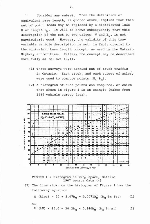
(2) A histogram of such points was computed, of which
that shown in Figure 1 is an example (taken from
1967 vehicle survey data).
10 0 0
�· ,. 255 259 .. ""' • z
"
12 18 14 5 3 6 29 4 I
zo •• •• EQUIVALENT BASE LENGTH S... W FU.T
•• ••
FIGURE 1 : Histogram in vl/BM space, Ontario 1967 census data (4)
60 ..
(3) The line shown on the histogram of Figure 1 has the
following equation
vi (kips) � 20 + 2. 07BH
- 0. 0071B� (BM
in ft.) (1)
or
V1 (kN) 89.0 + 30. 2BM
- 0.340B� (BM
in m.) (2)
3.
This curve, which lies some distance below the
upper bound of the survey data, is called the
"Ontario Bridge Formula" (OBF).
(4) A subsequent 1971 survey was used to establish a
virtual upper bound of vehicles in Ontario. This
revised curve, called the Maximum Observed Load
(MOL), is given by
MOL (kips) 42. 5 + 2. 07
or
MOL (kN) 189. 0 + 30. 2
B -M
(for
B -M
0. 0071 B� ( 3)
BM
in feet)
0. 340 Bz M
( 4)
(for BM
in metres).
(5) The results of the 1967 and 1971 surveys were
confirmed by a third, 1975 survey.
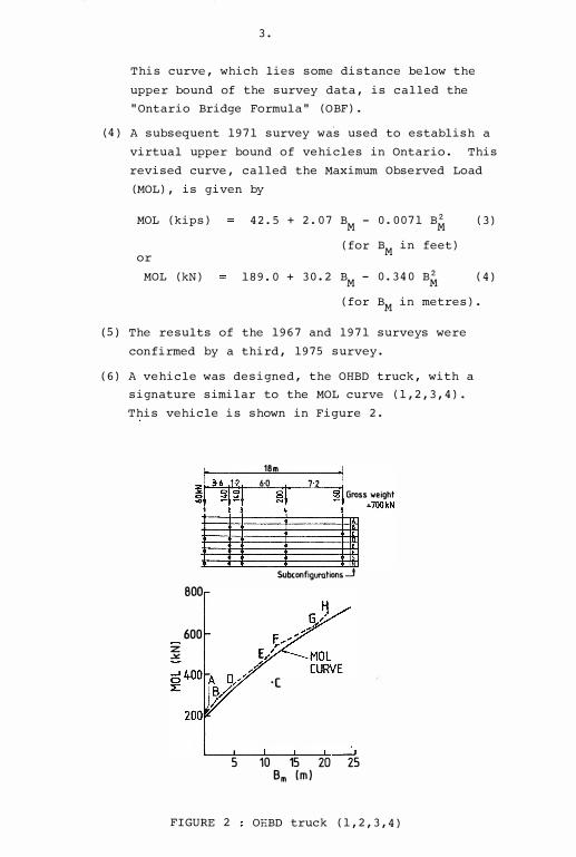
(6) A vehicle was designed, the OHBD truck, with a
signature similar to the MOL curve (1,2,3,4).
This vehicle is shown in Figure 2.
z .X
I 1am I ��l���� 60 �� 7 2 §j Gross weight
I II l II(� SubtonfigUI'Qtions .J
BOO
600
·(
5 10 15 20 25 Bm (m)
FIGURE 2 OEBD truck (1,2,3,4)
4.
The crucial questions raised by the above
procedure are as follows.
(a) Is it valid to replace survey data by a histogram
of points in (H, BM
) space?
(b) Is it valid to select a design vehicle on the
basis that its equivalent base length signature
follows a curve such as the MOL curve?
3. COMPUTATION OF THE ONTARIO EQUIVALENT BASE LENGTH
The method used for computing BM
is described fully
in reference 4. It is based on the criterion that the
equivalent distributed load produce the correct ab solute
maximum bending moment in a simply supported beam.
It will be recalled that the maximum bending moment
under a particular load of a group which is moved across
the span occurs when the centre of the span bisects the
distance between that particular load and the centre of
gravity of the load group.
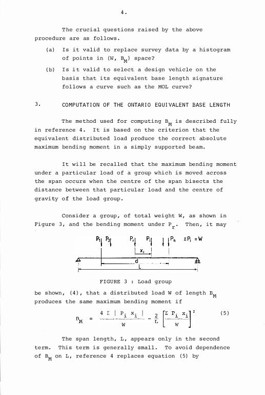
Consider a group, of total weight W, as shown in
Figure 3, and the bending moment under Pr
. Then, it may
EP; =W
d L
FIGURE 3 : Load group
be shown, (4), that a distributed load W of length BM
produces the same maximum bending moment if
4 z I Pi
xi I
w (5)
The span length, L, appears only in the second
term. This term is generally small. To avoid dependence
of BM
on L, reference 4 replaces equation (5) by
5.
(6)
The theorem quoted above does not identify the
load under which the absolute maximum bending moment occurs.
Reference 4 suggests that the load "closest to the centre
of gravity of the sequence" should be used.
4. ALTERNATIVE DERIVATION OF EQUIVALENT BASE LENGTH
4.1 Typical Influence Lines
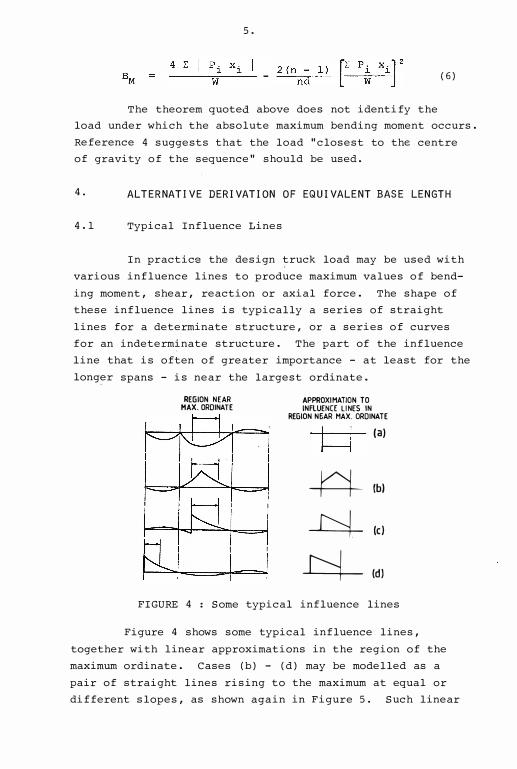
In practice the design truck load may be used with
various influence lines to produce maximum values of bend
ing moment, shear, reaction or axial force. The shape of
these influence lines is typically a series of straight
lines for a determinate structure, or a series of curves
for an indeterminate structure. The part of the influence
line that is often of greater importance - at least for the
longer spans - is near the largest ordinate.
REGION NEAR APPROXIMATION TO MAX. ORDINATE INFlUENCE LINES IN
Ff?'=l REGION NgAR MAX. ORDINATE
� (a) �I ��I I � (b) r==--I IF:il I
# I I� 1<=-1 (c) SL' , .
4--'===-' � (d)
FIGURE 4 : Some typical influence lines
Figure 4 shows some typical influence lines,
together with linear approximations in the region of the
maximum ordinate. Cases (b) - (d) may be modelled as a
pair of straight lines rising to the maximum at equal or
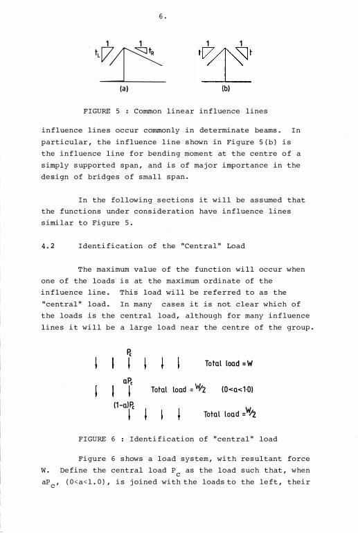
different slopes, as shown again in Figure 5. Such linear
6.
1 1 1 1 t,� 'T'
(a) (b)
FIGURE 5 : Common linear influence lines
influence lines occur commonly in determinate beams. In
particular, the influence line shown in Figure 5(b) is
the influence line for bending moment at the centre of a
simply supported span, and is of major importance in the
design of bridges of small span.
In the following sections it will be assumed that
the functions under consideration have influence lines
similar to Figure 5.
4.2 Identification of the "Central" Load
The maximum value of the function will occur when
one of the loads is at the maximum ordinate of the
influence line. This load will be referred to as the
"central" load. In many cases it is not clear which of
the loads is the central load, although for many influence
lines it will be a large load near the centre of the group.
Pc
I Total load =W
aPe
I Total load = W;z (0<a<1·0}
(1-alPc
I Total load ::W/2
FIGURE 6 Identification of "central" load
Figure 6 shows a load system, with resultant force
w. Define the central load Pc
as the load such that, when
aPe
, (O<a<l.O), is joined with the loads to the left, their
7.
resultant is !:!.2
. Similarly , (1-a) P with the loads to w c
the right also has resultant 2.
It will be shown that this definition of the
central load is correct for an equi- angular influence line
(i.e. as shown in Figure 4 (b)).
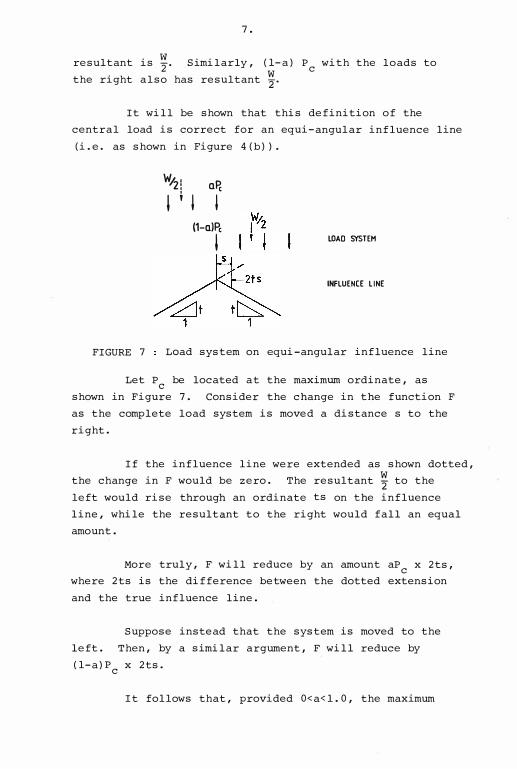
FIGURE 7
W,t.2:, P. Q c I ' I I
(1-alPc I LOAD SYSTEM
INFLUENCE LINE
Load system on equi-angular influence line
Let Pc
be located at the maximum ordinate, as
shown in Figure 7. Consider the change in the function F
as the complete load system is moved a distance s to the
right.
If the influence line were extended as shown dotted,
the change in F would be zero. The resultant � to the
left would rise through an ordinate ts on the influence
line, while the resultant to the right would fall an equal
amount.
More truly, F will reduce by an amount aPe
x 2ts,
where 2ts is the difference between the dotted extension
and the true influence line.
Suppose instead that the system is moved to the
left. Then, by a similar argument, F will reduce by
(1- a)Pc
x 2ts.
It follows that, provided O<a<l.O, the maximum
8.
value of F will occur with Pc
at the maximum ordinate.
It cannot be argued that the same load will be the
"central load" for an asy mmetric influence line. Rather
the validity of the above definition of the central load
will depend on the magnitude of a and the relative
magnitudes of the slopes tL
and tR
.
In the present argument, it is desirable to have
a unique definition of the central load. The definition
given above will be adopted as being correct for the
important case of an equi- angular influence line, and a
reasonable choice for many others in which the slope
difference is not great.
4.3 Ambiguous Case
The above definition of the central load is
ambiguous in the case where a = 0 (or 1.0). Pc
may be
identified by summing the loads from the left and stopping
when the sum is equal to or greater than w 2. If the sum
w equals 2, then either the current wheel, or that next to
the right, may be the central wheel.
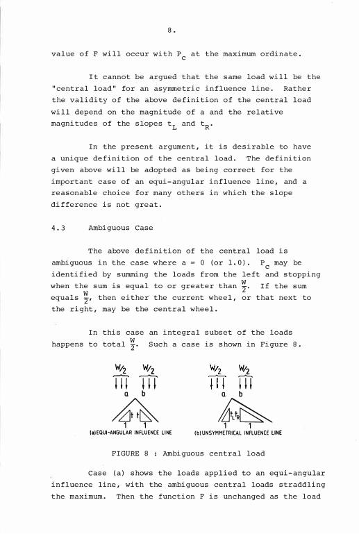
In this case an integral subset of the loads w
happens to total 2. Such a case is shown in Figure 8.
W;z W;z mm
Q b
� 1 1 (a)EQUI·ANGULAR INFLUENCE LINE
W!z m
Q b
� 1 1 (b) UNSYMMETRICAL INFLUENCE LINE
FIGURE 8 : Ambiguous central load
Case (a) shows the loads applied to an equi-angular
influence line, with the ambiguous central loads straddling
the maximum. Then the function F is unchanged as the load
9.
system is moved from load b at the maximum to load a at
the maximum. That is, in this case, either a or b may be
used as the central load.
This situation does not occur in Case (b). Here
it is clear that for tL
> tR
' the load system must be
moved to the right until load a is at the maximum. In
practice, a design truck load system may be reversed.
With this in mind the worst central load may be defined as
that one of the loads a and b which is the smaller distance w
from the resultant of its 2 group.
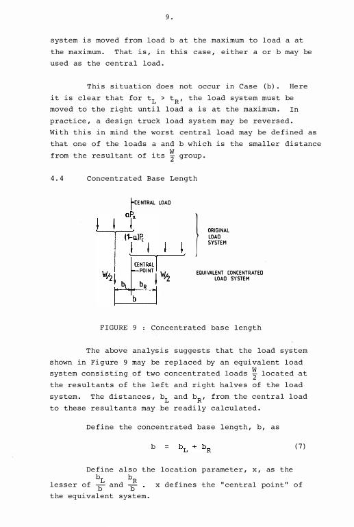
4.4 Concentrated Base Length
rCE NTRAL LOAD
aP.
) ORIGINAL
LOAD
SYSTEM
Tl'
' ':_JP. ___ , -----'-" CENTRAL�
W POINT W V2J b b ' � EQUIVALENT CONCENTRATED
LOAD SYSTEM
L R
FIGURE 9 Concentrated base length
The above analysis suggests that the load system
shown in Figure 9 may be replaced by an equivalent load
system consisting of two concentrated loads ; located at
the resultants of the left and right halves of the load
sy stem. The distances, bL
and bR
, from the central load
to these resultants may be readily calculated.
Define the concentrated base length, b, as
b (7)
Define also the location parameter, x, as the b
L b
R lesser of band b x defines the "central point" of
the equivalent system.
10.
This equivalent load system, when applied to any
linear influence line, will produce the same value of the
function F as the original system, provided that Pc and
the central point are both placed at the maximum ordinate.
It is worth repeating this conclusion. The
equivalent load system may be used to find a maximum value
of the function F, with the load system facing in either
direction, and with the central point at the maximum
ordinate. Then this maximum will be the same as for the
original load system, provided that the worst load (i. e.
the one at the maximum ordinate) is indeed that defined
above as the "central load".
4. 5 Relationship between the Concentrated Base Length and the Ontario Equivalent Base Length
It was noted previously that in the definition of
the Ontario equivalent base length, equation ( 5) or (6) ,
the second term was small. Suppose it is neglected.
Assume also that the central load, Pr' is as defined above.
Then, for the left hand group of loads,
l: I I w P. x. 2
bL. l. l.
Similarly, for the right hand group,
l: I P. w x. 2
bR
. l. l.
For the complete load system,
4 l: w
2b.
That is, the simplified value of BM is precisely
equal to twice the concentrated base length, subject only
to the restriction that the same central load must be
used.
11.
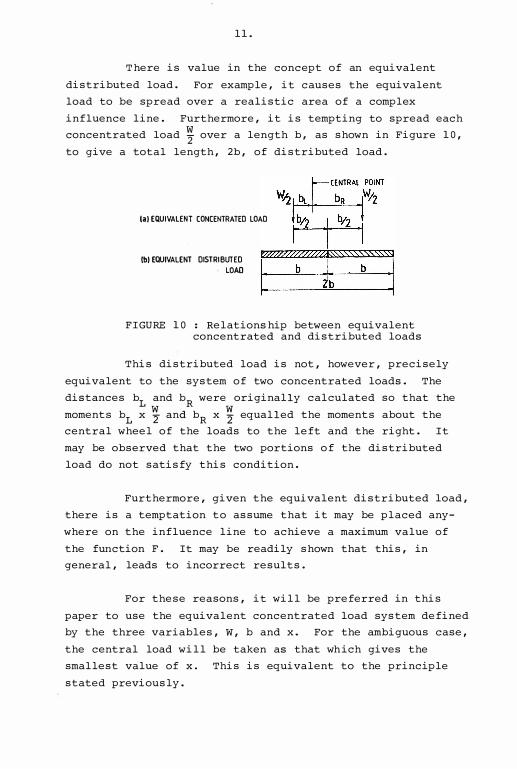
There is value in the concept of an equivalent
distributed load. For example, it causes the equivalent
load to be spread over a realistic area of a complex
influence line. Furthermore, it is tempting to spread each
concentrated load ; over a length b, as shown in Figure 10,
to give a total length, 2b, of distributed load.
(a) EQUIVALENT CONCENTRATED LOAD
(b) EQUIVALENT DISTRIBUTED LOAD
FIGURE 10 : Relations hip between equivalent concentrated and distributed loads
This distributed load is not, however, precisely
equivalent to the system of two concentrated loads. The
distances bL
and bR
were originally calculated so that the w w
moments bL
x 2 and bR
x 2 equalled the moments about the
central wheel of the loads to the left and the right. It
may be observed that the two portions of the distributed
load do not satisfy this condition.
Furthermore, given the equivalent distributed load,
there is a temptation to assume that it may be placed any
where on the influence line to achieve a maximum value of
the function F. It may be readily shown that this, in
general, leads to incorrect results.
For these reasons, it will be preferred in this
paper to use the equivalent concentrated load system defined
by the three variables, W, b and x. For the ambiguous case,
the central load will be taken as that wh ich gives the
smallest value of x. This is equivalent to the principle
stated previously.
12.
5 . VALIDITY O F THE EQUIVALENT BASE LENGTH
The equivalent loads described previously give
exact results only in some simple cases. It is desirable
to check the quality of the substitution for a range of
cases.
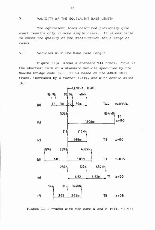
5. 1 Vehicles with the Same Base Length
Figure ll (a) shows a standard T44 truck. This is
the shortest form of a standard vehicle specified by the
NAASRA bridge code (5). It is based on the AASHO HS20
truck, increased by a factor 1. 349, and with double axles
(6) .
96196
1
tCENTRAL LOAD 96l 96l 4BkNI
(a) 11-21 3·0 11-2 1 37m I T44 x=0-3364
345·6, 86·4 kNj T1
(b) I 12·06m I X=O·O
216l
216kNI
(c) � T2 x=O·O
f9·6 259·2
1 43-2kN I
I 6·03 ·I 6·03m I T3 x=0·25
259·2'
129·6,
H2kNI
(d)
,J 4·82 I 4 · 82m I T4 x=O·O
1441 144kN I I
(e)
(f) I 3·62 .1 362m I T5 x=0·5
FIGURE ll Trucks with the same W and b (T44, Tl-T5)
13.
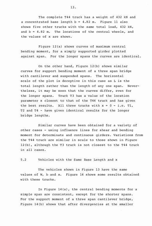
The complete T44 truck has a weight of 432 kN and
a concentrated base length b = 4. 82 m. Figure 11 also
shows five other trucks with the same total load, 432 kN,
and b = 4. 82 m. The locations of the central wheels, and
the values of x are shown.
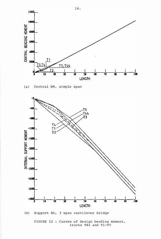
Figure 12 (a) shows curves of maximum central
bending moment, for a simply supported girder plotted
against span. For the longer spans the curves are identical.
On the other hand, Figure 12 (b) shows similar
curves for support bending moment of a three span bridge
with cantilever and suspended spans. The horizontal
scale of the plot is deceptive in this case as L is the
total length rather than the length of any one span. Never
theless, it may be seen that the curves differ, even for
the longer spans. Truck T3 has a value of the location
parameter x closest to that of the T44 truck and has given
the best results. All three trucks with x = 0 - i. e. Tl,
T2 and T4 - have given identical results for the longer
bridge lengths.
Similar curves have been obtained for a variety of
other cases - using influence lines for shear and bending
moment for determinate and continuous girders. Variations from
the T44 truck are similar in scale to those shown in Figure
12 (b) , although the T3 truck is not closest to the T44 truck
in all cases.
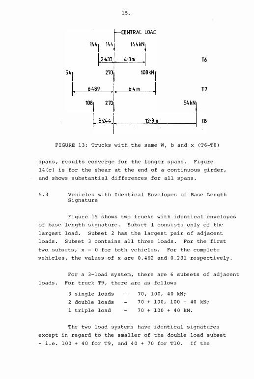
5 . 2 Vehicles with the Same Base Length and x
The vehicles shown in Figure 13 have the same
values of W, b and x. Figure 14 shows some results obtained
with these trucks.
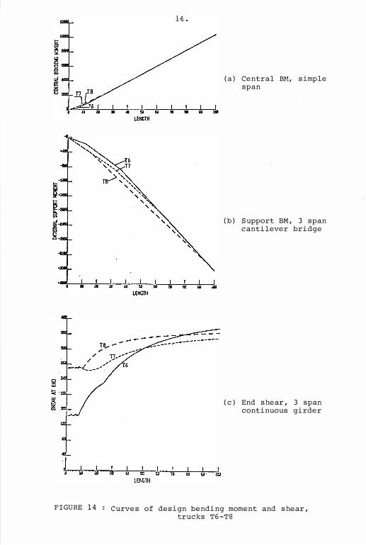
In Figure 14 (a) , the central bending moments for a
simple span are consistent, except for the shorter spans.
For the support moment of a three span cantilever bridge,
Figure 14 (b) shows that after divergencies at the smaller
14.
(a) Central BM, simple span
-1 1-
� §i -1 1-� C)
&:�
(b) Support Bt.l, 3 span cantilever bridge
FIGURE 12 : Curves of design bending moment, trucks T44 and Tl-T5
15.
T6
6·469
'"'I ";I· .. 54 k"l T7
�I �3�l�44�� -------1=2�·B=m�-------4· ' TB
FIGURE 13: Trucks with the same W, b and x (T6-T8)
spans, results converge for the longer spans. Figure
l4 (c) is for the shear at the end of a continuous girder,
and shows substantial differences for all spans.
5.3 Vehicles with Identical Envelopes of Base Length Signature
Figure 15 shows two trucks with identical envelopes
of base length signature. Subset l consists only of the
largest load. Subset 2 has the largest pair of adjacent
loads. Subset 3 contains all three loads. For the first
two subsets, x 0 for both vehicles. For the complete
vehicles, the values of x are 0.462 and 0.231 respectively.
For a 3- load system, there are 6 subsets of adjacent
loads. For truck T9, there are as follows
3 single loads
2 double loads
1 triple load
70, 100, 40 kN;
70 + 100, 100 + 40 kN;
70 + 100 + 40 kN.
The two load systems have identical signatures
except in regard to the smaller of the double load subset
- i.e. 100 + 40 for T9, and 40 + 70 for TlO. If the
/ /
!<·
t•
FIGURE 14
TB..- _.. ....
T6
(a) Central BH, simple span
(b) Support BM, 3 span cantilever bridge
(c) End shear, 3 span continuous girder
Curves of design bending moment and shear, trucks T6-T8
17.
signatures were truly identical, then the load systems as
a whole would become identical. Here the phrase has been
used because they have identical envelopes of base length
signature.
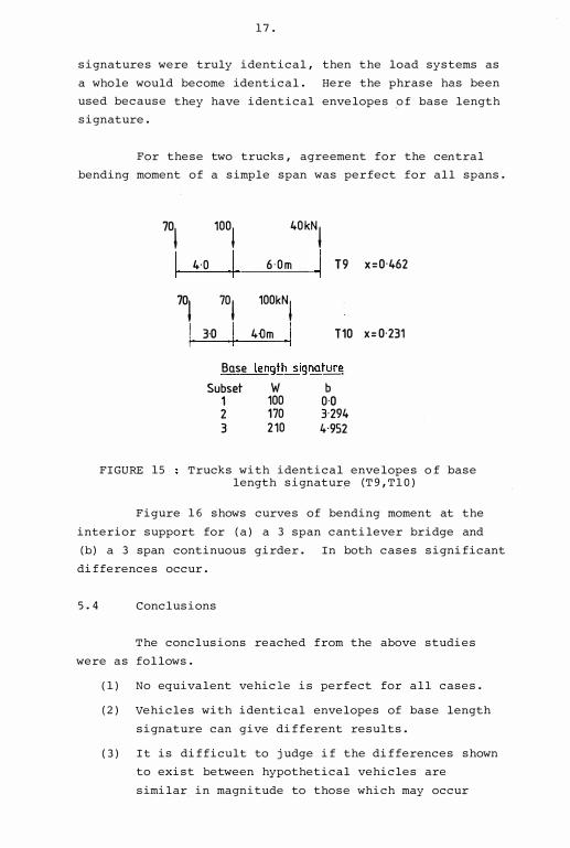
For these two trucks, agreement for the central
bending moment of a simple span was perfect for all spans.
70l
I 701
I
1001
4·0 I 70l
3-0 I Base
Subset 1 2 3
40kNl
6·0m I T9
100kNl
4-Dm I T10
length signature
w b 100 0·0 170 3·294 210 4·952
x=0·462
X:0·231
FIGURE 15 Trucks with identical envelopes of base length signatur� (T9, Tl0)
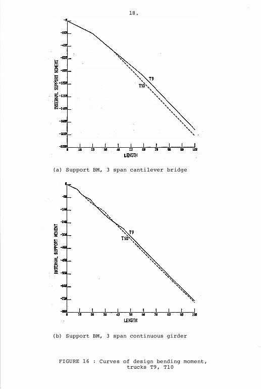
Figure 16 shows curves of bending moment at the
interior support for (a) a 3 span cantilever bridge and
(b) a 3 span continuous girder. In both cases significant
differences occur.
5. 4 Conclusions
The conclusions reached from the above studies
were as follows.
(1) No equivalent vehicle is perfect for all cases.
{2) Vehicles with identical envelopes of base length
signature can give different results.
(3) It is difficult to judge if the differences shown
to exist between hypothetical vehicles are
similar. in magnitude to those which may occur
� '
',
'
18.
' '
',
',·
'
T10' ',
',
, '
,,
' '
' '
' '
,, ' '
' '
' '
(a) Support BM, 3 span cantilever bridge
(b) Support BM, 3 span continuous girder
FIGURE 1 6 Curves of design bending moment, trucks T9, TlO
19.
with practical vehicles.
(4) There is some prospect of designing a satisfactory
equivalent vehicle by the use of the following
criteria -
(a) same maximum single axle load (or possibly
the same worst axle group);
(b) same envelope of base length signatures;
(c) for the total vehicle, the same total load,
concentrated base length, and location
parameter.
6. CHECK OF ONTARIO PROCEDURE
6. 1 Simulation Study
It was decided therefore to simulate the entire
Ontario process described in reference 4. The following
steps were taken.
(1) A series of vehicles was generated with configur
ations lying at the Australian legal limits. These vehicles
are illustrated in Figure 17 and may be described as
follows.
(a) there are 2, 3 or 4 axle groups;
(b) the front group has 1 or 2 axles; the other
axle groups have 1, 2 or 3 axles, except that the second
group is not permitted to have fewer axles than the first,
and the fourth group, if it exists, has the same number of
axles as the third;
(c) the spacing of adjacent axles for a 2 axle
group is 1. 2 m, and for a 3 axle group 1.0 m;
(d) the spacing of adjacent axles of groups 1 and
2 is 3 rn, and either 3 or 6 m for other groups;
(e) vehicles longer than 16 m between extreme
axles are excluded;
(f) the �eight of an axle group is, where possible,
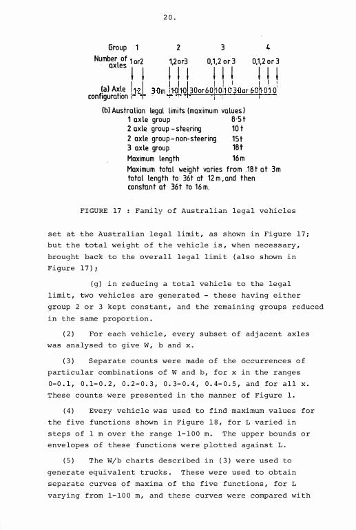
20.
Group 2 3
Numbi;l�I ti tr31 oy r i oy r I (al Ax!e 1,_21 lOrn 1-0 1{) 30or60ll0 !1 ol3{)or 6Dh ·0'1 0 conf1gurahon f.!4--' (b) Australian legal limits (maximum values l
1 axle group 8·5 t 2 axle group- steering 10 t 2 axle group-non-steering 1St 3 axle group 1Bt Maximum length 16m Maximum total weight varies from .1Bt at 3m total length to 36t at 12m,and then constant at 36t to 16 m.
FIGURE 17 : Family of Australian legal vehicles
set at the Australian legal limit, as shown in Figure 17;
but the total weight of the vehicle is, when necessary,
brought back to the overall legal limit (also shown in
Figure 17) ;
(g) in reducing a total vehicle to the legal
limit, two vehicles are generated - these having either
group 2 or 3 kept constant, and the remaining groups reduced
in the same proportion.
(2) For each vehicle, every subset of adjacent axles
was analysed to give W, b and x.
(3) Separate counts were made of the occurrences of
particular combinations of W and b, for x in the ranges
0-0. 1, 0. 1-0. 2, 0. 2 - 0. 3, 0. 3- 0. 4, 0. 4- 0. 5 , and for all x.
These counts were presented in the manner of Figure 1.
(4) Every vehicle was used to find maximum values for
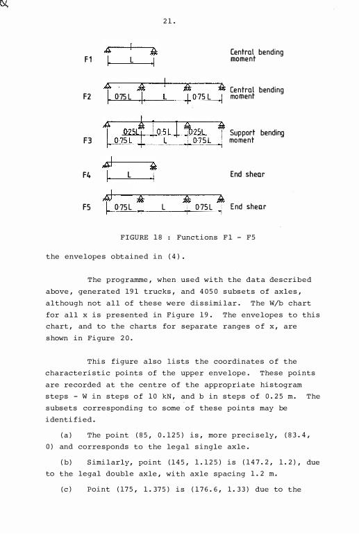
the five functions shown in Figure 18, for L varied in
steps of 1 m over the range 1-100 m. The upper bounds or
envelopes of these functions were plotted against L.
(5 ) The W/b charts described in (3) were used to
generate equivalent trucks. These were used to obtain
separate curves of maxima of the five functions, for L
varying from 1-100 m, and these curves were compared with
A A F 1 �I __,L"----1•1
A A F2 I 0·75 L I
F3
,J � F4 I L I
21.
L
AI £> F5 � 0·75l .� l
Central bending moment
A A Central bending 1 0·75 L 1 moment
;{,\: A
Support bending moment
End shear
1 0·75 L 1 End shear
FIGURE 18 : Functions Fl - F5
the envelopes obtained in (4).
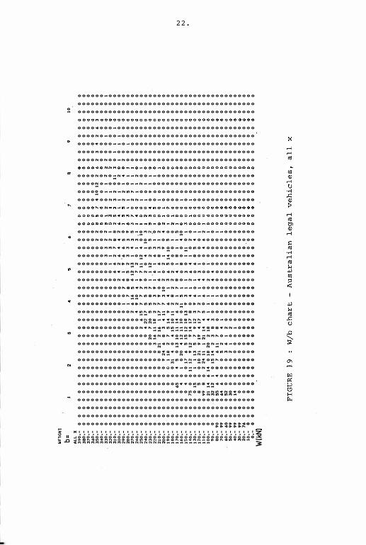
The programme, when used with the data described
above, generated 191 trucks, and 4050 subsets of axles,
although not all of these were dissimilar. The W/b chart
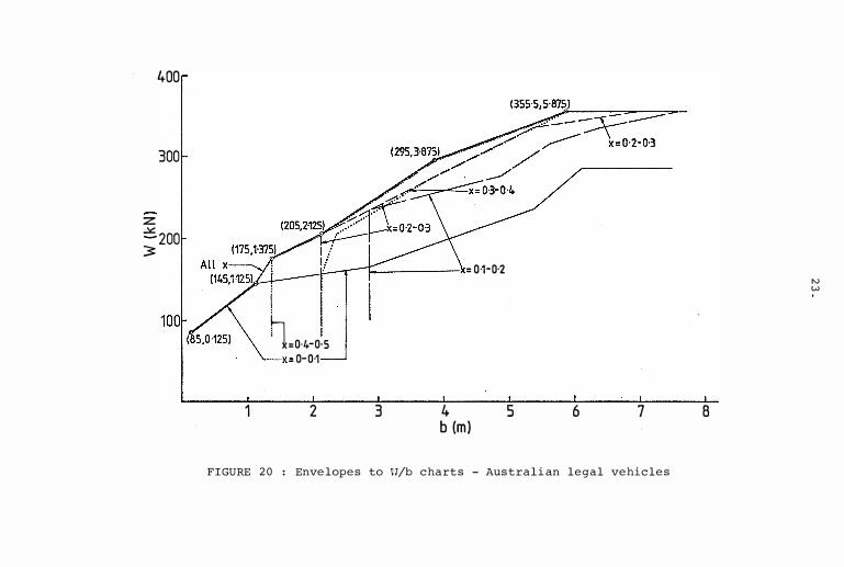
for all x is presented in Figure 19. The envelopes to this
chart, and to the charts for separate ranges of x, are
shown in Figure 20.
This figure also lists the coordinates of the
characteristic points of the upper envelope. These points
are recorded at the centre of the appropriate histogram
steps - W in steps of 10 kN, and b in steps of 0.25 m. The
subsets corresponding to some of these points may be
identified.
(a) The point (85' 0.125) is, more precisely, (83.4,
0) and corresponds to the legal single axle.
{ b) Similarly, point (145, 1.125) is (147.2, 1.2)' due
to the legal double axle, with axle spacing 1.2 m.
(c) Point (175, 1.375) is (176.6, 1. 33) due to the
I I L
22.
oooooo�ooooooooooooooooooooooooooooooooo
ooooooooooooooo�oooooooooooooooooooooooo
�·
oooooooooooooooooooooooooooooooooooooooo
oooo�ooo-ooooooooooooooooooooooooooooooo
ooooNo-oo-oooooooooooooooooooooooooooooo
ooo�•ooo--o-oooooooooooooooooooooooooooo
ooooMooo-ooooooooooooooooooooooooooooooo
OOOONONOO-NOOOOOOOOOOOOOOOOOOOOOOOOOOOOO
oooONONO:N•--Noo--oooooooooooooooooooooo
oooo�o-ooo-o--N--ooooooooooooooooooooooo
oooo�o--N-Nn�-oo�ooooooooooooooooooooooo
oooo•ooNM-N-NN--oo-oooo-o-oooooooooooooo
OOOONON-�NO�n��MN�N•00�2-o--N-o--OOOOOOO
ooooNONN�•nMMMo�n--on--•oN•o�ooooooooooo
ooooooMM�•�M•-•-nMM��o-o:ono•ooooooooooo
ooooooM�N��"�o�·N�m�:omo��mooooooooooooo
ooooooo��N�N:N:o���Nno�mo•��o�oooooooooo
ocoooooo�•�n���N��"o�N•o��o"oo•ooooooooo
OOOOOOOOON�m�"�O���N"NmO�N" •• N.OOOOOOOOO
oooooooooo�=n•�"��o2"N�"�"o�oooooooooooo
ooooooooooo����nm"�"•m"n"•�"���"oooooooo
0000000000"•••�nnN��·NN:•o•NOM0000000000
OOOOOOOOOOOON·��nN�=·:�o:m"�n"oOOOOOOOOO
oooooooooooooo����"·:�:�����·•"O•ooooooo
ooooooooooooOoN•�:�"n�::�:••:�=m•NN"oooo
oooooooooooooooog�Nm�•���·���N"�o-oooooo
oooooooooooooooooM"�No"•nNn•"oN•N�•ooooo N " " N M
oooooooooooooooooom��·og•�:N:�:�nMNooooo
ooooooooooooooooooo••Mno��-��o��oooooooo
ooooooooooooo·ooooooooo•-o:•oN:omoooooooo
ooooooooooooooooooooooooooooo•••oooooooo
oooooooooooooooooooooo�•·o�n=:���ooooooo
ooooooooooooooooooooooooonom�-Nn•No•oooo � �N"n�nMM
oooooooooooooooooooooooooooooooooooooooo
oooooooooooooooooooooooooooooooooooooooo
oooooooooooooooooooooooooooooooooooooooo
ooooooooooooooooooooooooooooooo�:�tt:�oo
II :��������l���������l�l�l���l��lll��l��ll�� � ��=�•n•MNMO�m�<n•"N�O�m�·��"NMO�m��n•MN" -¢M�MMMMMM"MNNNNNNNNNNMMMMMMMMMM �
400
300
z ==-200 3
= 0·1-0·2 r----1 1 I
! I � I i :0·4-0·5
X= 0-0·1
1 2 3 4 5 6 7 b (m)
FIGURE 20 : Envelopes to H/b charts - Australian legal vehicles
8
"' w
24.
legal triaxle, with axle spacings 1. 0 m.
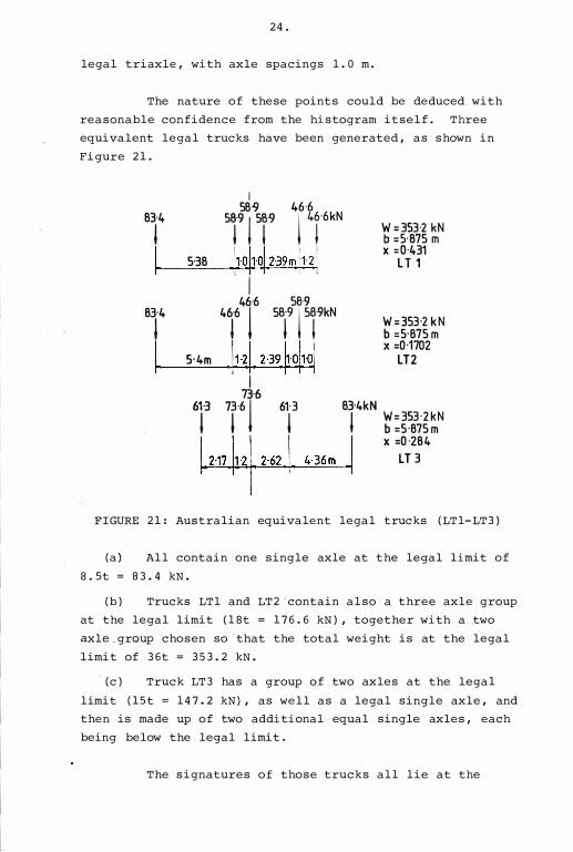
The nature of these points could be deduced with
reasonable confidence from the histogram itself. Three
equivalent legal trucks have been generated, as shown in
Figure 21.
I 58.1) 46·6 83·4 5rl
5r 14tkN ' W =353·2 kN b =5·875 m
I lwl,.ol2-39m 11·21 X :0·431 5·38 L T 1
I 46·6 58·9 83-4 4lu j
sy 15rkN W=353·2 kN l b =5·875m � j1-2j n9!1+nl X :0·1702
5·4m LT2
I 73-6 61-3
l61
61-3 83-4kN l l ' W=353-2kN
b =5·875m X :0·284
LT 3
FIGURE 21: Australian equivalent legal trucks (LT1-LT3)
(a) All contain one single axle at the legal limit of
B. St : 83. 4 kN.
(b) Trucks LTl and LT2 ·contain also a three axle group
at the legal limit (1St : 176.6 kN), together with a two
axle group chosen so that the total weight is at the legal
limit of 36t : 353. 2 kN.
(c) Truck LT3 has a group of two axles at the legal
limit (1St : 147.2 kN), as well as a legal single axle, and
then is made up of two additional equal single axles, each
being below the legal limit.
The signatures of those trucks all lie at the
25.
envelope for all x shown in Figure 20. This figure shows
that the envelopes of W tend to rise as x increases. That
is, there is a presumption that the vehicle which will best
simulate the worst legal truck will have a high value of x.
Figure 21 lists x for the three complete vehicles. LTl has
the largest x and on this principle should be preferred.
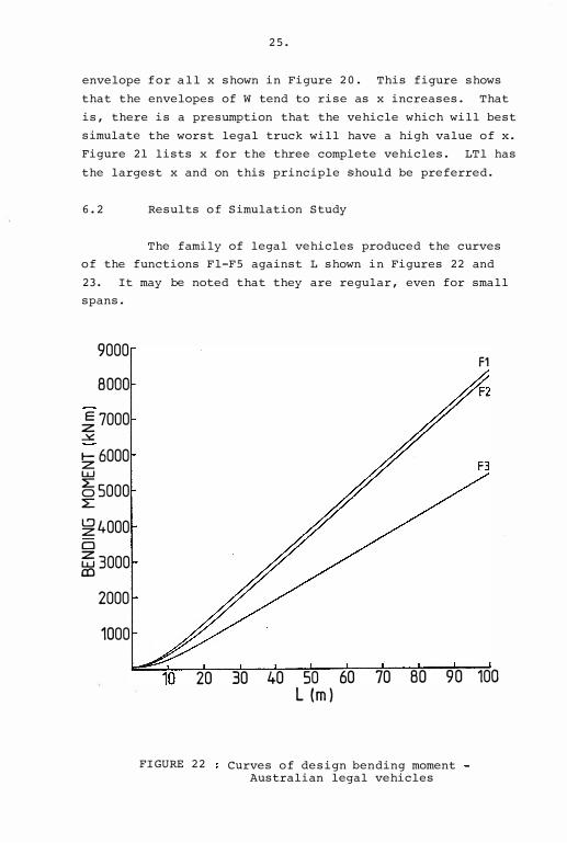
6. 2 Results of Simulation Study
The family of legal vehicles produced the curves
of the functions Fl-F5 against L shown in Figures 22 and
23. It may be noted that they are regular, even for small
spans.
9000 BODO
�7000 �
�6000 LU �5000 L:
�4000 D �3000
2000 1000
F1
20 30 40 50 60 70 80 90 100 L(m)
FIGURE 22 Curves of design bending moment Australian legal vehicles
340
300
260
-220 z ...lo::
0::: 180
<( �140 V)
10
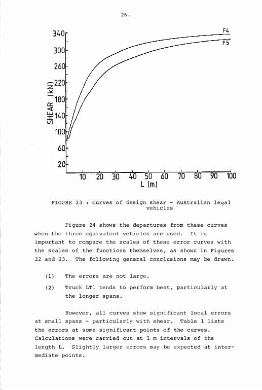
FIGURE 23
20 30
26.
40 50 60 L (ml
70
F4
FS
BO 90 100
Curves of design shear - Australian legal vehicles
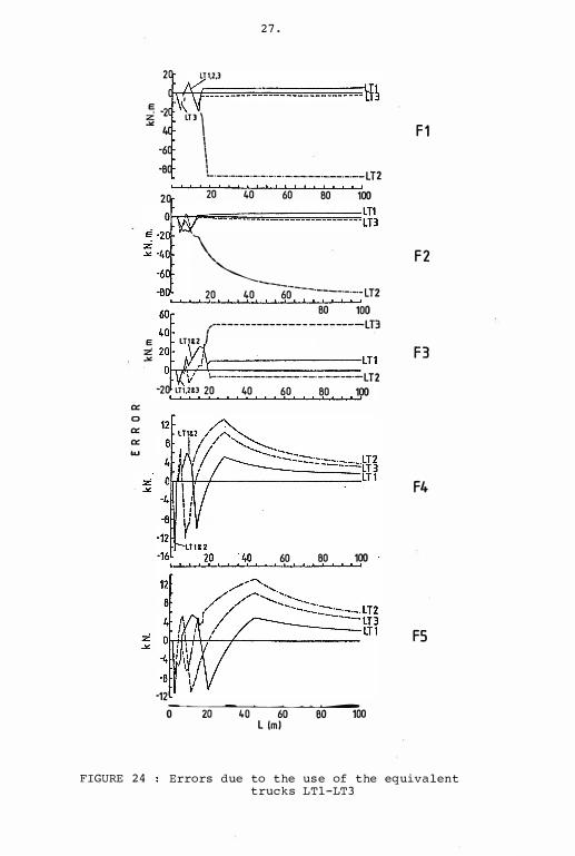
Figure 24 shows the departures from these curves
when the three equivalent vehicles are used. It is
important to compare the scales of these error curves with
the scales of the functions themselves, as shown in Figures
22 and 23 . The following general conclusions may be drawn.
(1) The errors are not large.
(2 ) Truck LTl tends to perform best, particularly at
the longer spans.
However, all curves show significant local errors
at small spans - particularly with shear. Table 1 lists
the errors at some significant points of the curves.
Calculations were carried out at 1 m intervals of the
length L. Slightly larger errors may be expected at inter
mediate points.
"'
0
"'
"' ...
20 LT1.2,3
27.
0 I
----------------------------- LH e •\ � -: Lll \
e :Z .>::
-60 -80
20
\ L.-·-·--·-·-·-·-·-· -·-·-·-·-·-·--·-·--LT2
20 40 60 80 100
" "----
20 40 -6o--·-·---·-·--m 80 100
,---------------- --------LT3 I
LT1&2 I
\r----------LT1 V \....·-·-·--·---·-----·--· -·-·---·-LT2
-20 LT1,2&3 20 40 60 80 100
60 80 100
-12 0���2�0��40���60���80��100
L (m)
F1
F2
F3
F4
FS
FIGURE 24 Errors due to the use of the equivalent trucks LT1-LT3
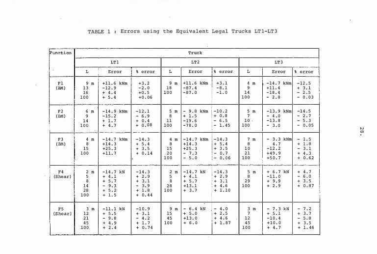
TABLE 1 Errors using the Equivalent Legal Trucks LT1-LT3
!Function Truck
LT1 LT2 LT3
L Error % error L Error % error L Error F1 9 m +11. 6 kNm +3.2 9 m +11. 6 kNm . +3.1 4 m - 14.7 kNm
(BM) 13 - 12.9 - 2.0 18 - 87.4 - 8.1 9 +11. 4 16 + 4.4 +0.5 100 - 87.0 - 1.0 14 - 18.4
100 + 5.4 +0.06 100 - 2.8
F2 6 m - 14.9 kNm - 12.1 5 m - 9.8 kNm - 10.2 5 m - 13.9 kNm
(BM) 9 - 15.2 - 6.9 8 + l. 5 + 0.8 7 - 4 •. 0 14 + l. 7 + 0.4 11 - 19.6 - 6.5 10 ' - 13.8
100 + 4.7 + 0.08 100 - 78.0 - l. 45 100 - 3.0
F3 4.
m - 14.7 kNm - 14.3 4 m - 14.7 kNm - 14.3 7 m - 3.3 kNm
(BM) 8 +14.3 + 5.4 8 +14.3 + 5.4 8 4.7 15 +25.3 + 3.5 15 +25.3 + 3.5 10 - 12.2
100 +11. 7 + 0.14 20 - 7.3 - 0.7 21 +49.9 100 - 5.0 - 0.06 100 +50.7
F4 2 m - 14.7 kN - 14.3 2 m - 14.7 kN - 14.3 5 m + 6.7 kN (Shear) 5 + 4.1 + 2.9 5 + 4.1 + 2.9 8 - 11.0
8 + 5.7 + 3.1 8 + 5.7 + 3.1 29 + 9.9 14 - 9.3 - 3.9 28 +13.1 + 4.6 100 + 2.9 28 + 5.2 + 1. 8 100 + 3.7 + 1.10
100 + l. 5 + 0.44
F5 3 m - 11.1 kN - 10.9 9 m - 6.4 kN - 4.0 3 m - 7.3 kN (Shear) 12 + 5.5 + 3.1 15 + 5.0 + 2.5 7 + 5.1
21 - 9.8 - 4.2 45 +13.0 + 4.6 12 - 10.4 45 + 4.9 + 1. 7 100 + 6.0 + l. 87 45 +10.0
100 + 2.4 + 0.74 100 + 4.7
% error - 12.5 + 3.1 - 2.5 - 0.03
- 14.5 - 2.7 - 5.3 - o. 05
- 1. 5 + 1.8 - 3.1 + 4.3 + 0.62
+ 4.7 - 6.0 + 3.5 + 0.87
- 7.2 + 3.7 - 5.8 + 3.5 + l. 46
N CX)
29,
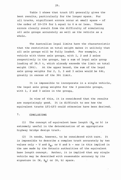
Table 1 shows that truck LTl generally gives the
best results, particularly for the longer spans. For
all trucks, significant errors occur at small spans - of
the order of 10- 15% for L equal to 6 m or less. These
errors clearly result from the difficulty of simulating
all axle groups accurately as well as the vehicle as a
whole.
The Australian legal limits have the characteristic
that the restriction on total weight makes it unlikely that
all axle groups will be fully loaded. For example, a
vehicle with three axle groups, with 1, 2 and 2 axles
respectively in the groups, has a sum of legal axle group
loading of 38.5 t, which already exceeds the limit on total
weight (36t). At the upper bound, the sum of the legal
axle group weights for 2, 3, 3 and 3 axles would be 64t,
greatly in excess of the 36t limit.
It is impossible to incorporate in a single vehicle,
the legal axle group weights for the 3 possible groups,
with l, 2 and 3 axles in the groups.
In view of this, it is considered that the results
are surprisingly good. It is difficult to see how the
equivalent trucks LT1-LT3 could otherwise have been derived.
7. CONCLUSIONS
(1) The concept of equivalent base length (BM
or b) is
extremely useful in the determination of an appropriate
highway bridge design truck.
(2) It needs, however, to be considered with care. It
is impossible to describe a complex truck accurately by two
values only - H and BM
' or H and b - nor is this implied in
the use made by the Ontario authorities of the equivalent
base length concept. Rather, it is implied that any single
vehicle may be described with reasonable accuracy by its
signature in {l'i', BM
) or (;'l, b) space.
30.
(3) This paper develops an equivalent concentrated
base length (b) . Although this differs from the Ontario
distributed base length (BM) , these differences do not
have significant practical consequences. The concentrated
base length is precisely 0. 5 x an approximate form of the
Ontario Equivalent Base Length.
( 4) The description of a subset of axles may be
enlarged to include a location parameter, x, and this may
be used to choose between equivalent vehicles with similar
base length signatures.
( 5) A study using a family of hypothetical Australian
legal vehicles shows that the Ontario method may be used
to choose equivalent vehicles which give accurate curves
against span of the maxima of five functions - (a) bending
moment at mid-span of a simply-supported girder, (b) bending
moment at mid-span of a 3-span continuous girder, (c) bend
ing moment at the support of a 3-span cantilever/suspended
span girder, (d) shear at the end of a simple girder, and
(e) shear at the end of a continuous girder. It may be
expected that similar accuracies would be achieved in other
cases.
(6) This study should also assist the selection of
an improved Australian design vehicle. It is proposed to
extend the study to investigate the effects of possible
changes in the Australian legal limits - particularly in
the specification of total mass or weight.
(7) The present AASHO design truck has a variable back
axle spacing. With the new OHBD truck, the designer is
required to consider various subsets of axles. The present
study suggests that it may be possible to use a single,
non-variable vehicle with sufficient accuracy. This would
lead to a reduction in the time involved in the computation
of design parameters, such as bending moment and shear.
This may be of particular value in computer-aided design,
where the use of variable vehicles can add significantly
to logical complexity and computation time.
8 • ACKNO\�LEDGEMENTS
31.
This study has arisen from work which has been
carried out at the University of Queensland on project
P321 of the Australian Road Research Board. This is part
of a more general study of truck loads in Australia.
Some of the computations were performed by Neville Richter,
Tutor in Civil Engineering. The paper has been typed by
Eileen Hoare.
l_
APPENDIX A
a
b
n
OBF
p c
s
t
32.
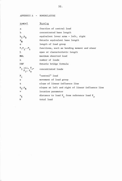
NOMENCLATURE
fraction of central load
concentrated base length
equivalent lever arms - left, right
Ontario equivalent base length
length of load group
functions, such as bending moment and shear
span or characteristic length
maximum observed load
number of loads
Ontario bridge formula
concentrated loads
"central" load
movement of load group
slope of linear influence line
slopes at left and right of linear influence line
location parameter
distance to load Pi
from reference load Pr
total load
33.
APPENDIX B REFERENCES
1. Ontario Highway Bridge Design Code 1979, Ontario Ministry of Transportation and Communications, Jan. 1979.
2. Ontario Highway Bridge Design Code 1979, Vol. II, Ontario Ministry of Transportation and Communications.
3. CSAGOLY, P.F., DORTON, R.A., "The Development of the Ontario Bridge Code", Ontario Ministry of Transportation and Communications, Oct. 1977.
4. CSAGOLY, P.F., DORTON, R.A., " Truck Weights and Bridge Design Loads in Canada", paper presented at the AASHTO Annual· Meeting, Louisville, Kentucky, Nov. 1, 1978.
5. NAASRA Bridge Design Specification, National Association of Australian State Road Authorities, Sydney, 1976.
6. American Association of State Highway Officials, Standard Specifications for Highway Bridges, 11th ed., 1973.
CE No.
l.
2.
3.
4.
5.
6.
7.
8.
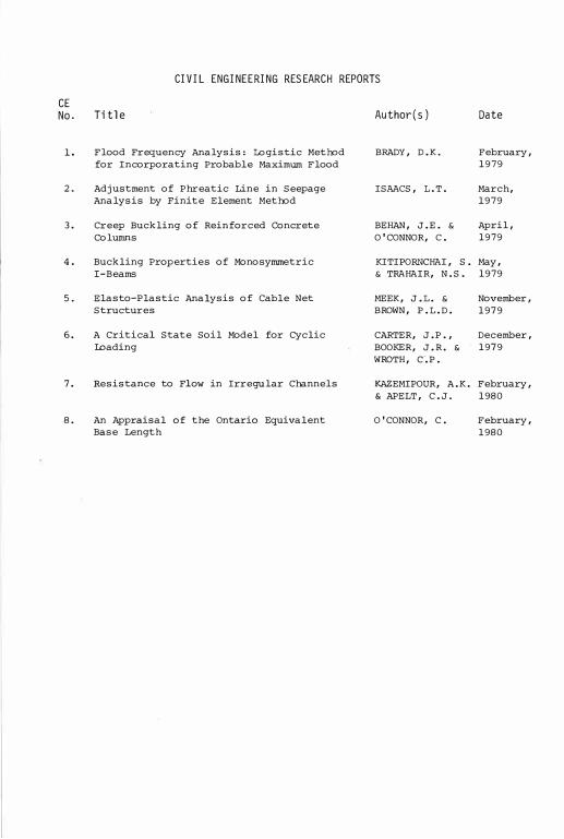
CIVIL ENGINEERING RESEARCH REPORTS
Title
Flood Frequency Analysis: Logistic Method
for Incorporating Probable Maximum Flood
Adj ustment of Phreatic Line in Seepage
Analysis by Finite Element Method
Creep Buckling of Reinforced Concrete
Columns
Buckling Properties of Monosyrnrnetric
!-Beams
Elasto-Plastic Analysis of Cable Net
Structures
A Critical State Soil Model for Cyclic
IDading
Resistance to Flow in Irregular Channels
An Appraisal of the Ontario Equivalent
Base Length
Author(s)
BRADY, D.K.
ISAACS, L.T.
BEHAN, J.E. &
O'CONNOR, C.
Date
February,
1979
March,
1979
April,
1979
KITIPORNCHAI, S. May,
& TRAHAIR, N.S. 1979
MEEK, J .L. &
BROWN, P.L.D.
CARTER, J.P.,
BOOKER, J.R. &
WROTH, c·.P.
November,
1979
December,
1979
KAZEMIPOUR, A.K. February,
& APELT, C.J. 1980
O'CONNOR, C. February,
1980
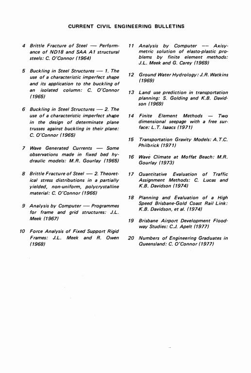
CURRENT CIVIL ENGINEERING BULLETINS
4 Brittle Fracture of Steel - Perform
ance of ND 18 and SAA A 1 structural
steels: C. O'Connor ( 1964)
5 Buckling in Steel Structures - 1. The
use of a characteristic imperfect shape
and its application to the buckling of
an isolated column: C. O'Connor
( 1965)
6 Buckling in Steel Structures - 2. The
use of a characteristic imperfect shape
in the design of determinate plane
trusses against buckling in their plane:
C. O'Connor ( 1965)
7 Wave Generated Currents - Some
observations made in fixed bed hy
draulic models: M.R. Gourlay ( 1965)
8 Brittle Fracture of Steel - 2. Theoret
ical stress distributions in a partially
yielded, non-uniform, polycrystalline
material: C. O'Connor ( 1966)
9 Analysis by Computer - Programmes
for frame and grid structures: J.L.
Meek ( 1967)
10 Force Analysis of Fixed Support Rigid
Frames: J.L. Meek and R. Owen
( 1968)
1 1 Analysis by Computer -- Axisy· metric solution of elasto-plastic problems by finite element methods: J.L. Meek and G. Carey ( 1969)
12 Ground Water Hydrology: J.R. Watkins
( 1969)
13 Land use prediction in transportation planning: S. Golding and K.B. Davidson ( 1969)
14 Finite Element Methods Two dimensional seepage with a free surface: L. T. Isaacs ( 197 1)
15 Transportation Gravity Models: A. T.C.
Philbrick ( 197 1)
16 Wave Climate at Moffat Beach: M.R.
Gourlay ( 1973)
17 Quantitative Evaluation of Traffic
Assignment Methods: C. Lucas and K.B. Davidson ( 1974)
18 Planning and Evaluation of a High Speed Brisbane-Gold Coast Rail Link:
K.B. Davidson, et at. ( 1974)
19 Brisbane Airport Development Flood
way Studies: C.J. Apelt ( 1977)
20 Numbers of Engineering Graduates in
Queensland: C. O'Connor ( 1977)