faculty of science and engineering

mathematics and applied mathematics

An application of Tauber theory: proving the Prime Number Theorem

Bachelor’s Project Mathematics

February 2018

Student: J. Koolstra

Supervisors: Prof.dr. J. Top and Dr. A. Sterk

Abstract

We look at the origins of Tauber theory, and apply it to prove theprime number theorem (PNT). Specifically, we prove a weak versionof the Wiener-Ikehara Tauberian theorem due to Newman. Its appli-cation requires us to establish some properties of the Riemann zetafunction. Most notably with regard to its meromorphic continuation,and the distribution of its zeros.

2

Contents

Introduction 5

Discrete Tauber theory 7Summability methods . . . . . . . . . . . . . . . . . . . . . . . . . 7The theorems of Tauber and Hardy-Littlewood . . . . . . . . . . . 13

The Wiener-Ikehara theorem 19Some complex analytic technicalities . . . . . . . . . . . . . . . . . 19A proof of the Wiener-Ikehara theorem . . . . . . . . . . . . . . . 19

The Riemann zeta function 28The meromorphic continuation of the zeta function . . . . . . . . . 28The zeta function is nonzero on the line Re z = 1 . . . . . . . . . . 32

The prime number theorem 37The linear bound on the Tchebychef ψ-function . . . . . . . . . . . 37Equivalent formulations of PNT . . . . . . . . . . . . . . . . . . . 39

Appendix A: the prime polynomial theorem 42

References 48

3

Even before I had begun my more detailed investigationsinto higher arithmetic, one of my first projects was toturn my attention to the decreasing frequency of primes,to which end I counted primes in several chiliads. I soonrecognized that behind all of its fluctuations, thisfrequency is on average inversely proportional to thelogarithm.

Gauss to Encke, 1849

It is not knowledge, but the act of learning, notpossession but the act of getting there, which grants thegreatest enjoyment. When I have clarified and exhausteda subject, then I turn away from it, in order to go intodarkness again. The never-satisfied man is so strange; ifhe has completed a structure, then it is not in order todwell in it peacefully, but in order to begin another. Iimagine the world conqueror must feel thus, who, afterone kingdom is scarcely conquered, stretches out his armsfor others.

Gauss to Bolyai, 1808

ὑμεῖς τε γὰρ οἱ λέγοντες μάλιστ᾿ ἂνοὕτως ἐν ἡμῖν τοῖς

ἀκούουσιν εὐδοκιμοῖτε καὶ οὐκ ἐπαινοῖσθε—εὐδοκιμεῖνμὲν

γὰρ ἔστιν παρὰ ταῖς ψυχαῖς τῶν ἀκουόντων ἄνευ ἀπάτης,

ἐπαινεῖσθαιδὲ ἐν λόγῳ πολλάκις παρὰ δόξαν ψευδομένων.

Prodicus in the Protagoras

4

Introduction

Tauber theory grew out of a single observation of A. Tauber (1866-1942)in 1897. He proved a nontrivial condition under which Abel summabilityimplies ordinary summability. The necessity of such a condition had alwaysbeen obvious, because Abel summability is easily seen to be stronger thanordinary summability, but a neat explicit formulation of it was new. Nowthe quest was on to establish more and stronger similar results.

The famous collaborators G. H. Hardy (1877–1947) and J. E. Littlewood(1885–1977) were the first to pick up on the result and realize its potentialas a representative of a general theory. They were intrigued by the idea andtogether set out to derive many related but much more intricate Tauber typetheorems. In particular, in 1911, Littlewood significantly weakened the as-sumption of Tauber’s original result, and later in 1914, together with Hardy,proved a nontrivial condition for moving from Abel summability to the morerestrictive Cesaro summability. They dubbed these results “Tauberian the-orems”, antonymic to the well known Abelian theorems.

In 2004, J. Korevaar published an article “A simple proof of the primenumber theorem” [1] that surveys the modification of Newman’s 1980 simpleproof of the prime number theorem (PNT) that we shall primarily study.1

PNT states that the number of primes under x is asymptotically distributedas x/ log x. In the article, Newman’s method is adapted to prove a weakversion of the Wiener-Ikehara Tauberian theorem. With the knowledge ofthe Riemann zeta function and Tchebychef’s ψ-function that we develop,this theorem is strong enough to imply PNT.

Korevaar explains that in particular number theory, and especially thesearch for simpler proofs of the prime number theorem, have formed a majorimpetus for the development of a more general Tauber theory. The directionwe take in this thesis to highlight Tauber theory therefore presents a naturalapproach. Tauber theory has developed in the past century into a wellestablished field of research, with many more deep results and techniquesthat are far beyond our scope. Indeed, the prime number theorem is onlythe start.

We proceed as follows. In the next section we introduce the conceptof summability and then focus on the summability methods of Cesaro andAbel. We also prove how these methods can be related using the Tauberiantheorems of Tauber and Hardy-Littlewood. In the subsequent section our

1The article is in Dutch. It appeared on the occasion of the publication of Korevaar’ssurvey book on Tauber theory, “Tauberian theory, a century of developments”.

5

attention shifts from the discrete to the continuous, and we derive a weakversion of the Wiener-Ikehara theorem, dubbed the “poor man’s” Wiener-Ikehara theorem. It forms the main body of the thesis, and most of thehard work. Then we are ready to prove the prime number theorem. We doso in two parts. First we derive all the essential properties of the Riemannzeta function that we need, featuring most prominently its meromorphiccontinuation to the complex plane, and its non-vanishing on the boundaryline of its natural domain of definition. Finally we combine all the ingredientsof the preceding sections, and finish the proof of the prime number theoremby relating it to the Tchebychef ψ-function.2

2With regard to prerequisites, it suffices to read, for example, Stein and Shakarchi [2],chapters I through III. Most importantly, one should know a bit about holomorphic func-tions and their basic properties, like analyticity, and having a unique analytic continuation.Assumed is Cauchy’s theorem, and Cauchy’s integral formula.

6

Discrete Tauber theory

We begin with a brief introduction of the concept of summability, and thenquickly focus on the summability methods of Cesaro and Abel (Definition1 and 3 respectively). Most importantly we prove that in a precise senseAbel summability is stronger than Cesaro summability (Theorem 1). Wealso prove how these methods can be related the other way around, and toordinary summability, using the (discrete) Tauberian theorems of Tauber,Littlewood and Hardy-Littlewood (resp. Theorem 2, 4 and 3).

Summability methods

Techniques for assigning to (divergent) series reasonable sums are calledsummability methods. Taken together they allow us to form a notion ofsummability that can function as an object of study in itself. The mostnatural and common such summability method is to assign to a series thelimit of its partial sums, as in calculus. Generalized concepts of summabil-ity, and older attempts thereon, grew out of an interest in divergent serieswith an appealingly simple structure or natural occurrence. Such seriesarise for example as formal solutions to certain differential equations, or bypondering over the meaning of sums like 1 + 1 + 1 + · · · . Interestingly, spe-cialized summability methods have found use beyond the pure mathematicalin theoretical physics.

Before Cauchy, Bolzano and Weierstrass introduced modern rigor inanalysis, and so for the first time offered precise definitions of intuitive con-cepts like convergence and divergence, divergent series had been the subjectof various intense debates. Indeed, the treatment of divergent series priorto the formalization of these foundations early in the nineteenth century,had mostly relied on a kind of heuristic reasoning that was notoriously in-tractable. It led Abel to conclude in 1826 that “divergent series are aninvention of the devil”. Afterwards, as a result of this widespread senti-ment, that was promulgated by the certainty of the new rigor, it took asurprisingly long time before someone dared to get involved with divergentseries again, and therefore also for the modern concept of summability toappear. The most notable such new involvement, in which this concept ismade explicit, is undoubtedly Hardy’s 1949 book “Divergent series”. In itspreface, his student Littlewood remarks that “in the early years of the cen-tury the subject, while in no way mystical or unrigorous, was regarded assensational, and about the present title, now colorless, there hung an aromaof paradox and audacity”.

7

A prototypical example of an appealing divergent series is the Grandiseries 1−1 + 1−1 + · · · .3 It diverges; but that is not a very mathematicallysatisfying conclusion. Would it not be more natural to make sense of thesum as the average position of the partial sums, jumping between 0 and 1,and assign it the sum 1/2? And if we agree on this assignment, can we thenfit it in a more general framework, that handles more such diverging series?In fact, this is precisely Cesaro summation, the first important summabilitymethod we look at.

Definition 1 (Cesaro summability). Given is a sequence of numbers an1≤n<∞with partial sums sn =

∑nk=1 ak. We define the new sequence

σn =1

n

n∑k=1

sk

that averages over these partial sums. If the limit limσn = A exists, we saythat the formal series

∑an is Cesaro summable, and assign it the limit A,

called the Cesaro sum of the series.

In contrast, we refer to the usual interpretation of series as according tothe ordinary summability method. It is easily verified that the Grandi seriesis indeed Cesaro summable with sum 1/2.

Without proof let us now make a simple yet prototypical observation.

Observation 1. Ordinary summability implies Cesaro summability. More-over, if a series can be ordinarily summed, then both methods assign thesame value to that series.

Some terminology is in place. We will not need all of it, but it is usefulto know some in order to get acquainted with how we would like to inter-act mathematically with summability methods. How to think about themeffectively, and how to organize them by their characteristics.

A summability method Σ, sometimes referred to as Σ-summation, is de-fined as a (partial) function that maps sequences of numbers (from CN) intothe complex plane. In the context of Σ we identify these sequences with theseries they formally define. For example we may reference the series

∑an

as S, and then identify Σ(S) with Σ(an). In this case S does not referto the outcome of the series, which might not even exist, but rather to the

3Wikipedia has a fairly good coverage of the interesting history of the Grandi series,maintained on the page “History of the Grandi series”. It is quite representative of theattitude towards divergent series during the various historical periods discussed.

8

series as an object itself. So even Σ(∑an) has an unambiguous and intuitive

meaning.We introduce the following convenient jargon, in line with the terminol-

ogy presented for Cesaro summability.

Definition 2 (A dictionary of summability). If a series S is in the domainof Σ, we say that it is Σ-summable and call Σ(S) the Σ-sum of the series.We sometimes also say that Σ sums the series S to the sum Σ(S). Fur-thermore, we isolate and name the following useful general properties that asummability method might have.

1. Regularity. If Σ sums all ordinarily convergent series to their ordinarysum, it is called regular.

2. Linearity. Let S and T be series summed by Σ and c some constant.We say that Σ is linear if cS + T is Σ-summable and Σ(cS + T ) =cΣ(S) + Σ(T ).

3. Stability. The method Σ is called stable if we can shift the initialterms of a series like Σ(

∑∞n=0 an) = Σ(

∑∞n=1 an) + a0.

In addition, suppose Π is another summability method, then Σ-summationis said to conserve Π if it sums all series summed by Π to their Π-sum. Soregularity is nothing else than the conservation of ordinary summation. Also,if in addition Σ sums any other series not summed by Π, then Σ is calledstronger than Π.

The notion of conservation induces a partial ordering on the set ofsummability methods. This gives rise to the shorthands Π Σ and Π ≺ Σfor the above concepts.

We can now succinctly state an improved observation about Cesaro sum-mation.

Observation 2. Cesaro summability is stronger than ordinary summability.Moreover, it is linear and stable.

Next we turn to Abel summation, the other important summabilitymethod we discuss.

Definition 3 (Abel summability). Given is a sequence of numbers an0≤n<∞.We define for 0 ≤ r < 1 the family of Abel means A(r) as the power series

A(r) =

∞∑n=0

anrn .

9

If all Abel means exist and converge to some value A as r → 1−, then∑an

is said to be Abel summable to A.

The goal of the remainder of this subsection is to prove the next theo-rem, and simultaneously relate Abel summation to the idea behind Cesarosummability.

Theorem 1. Abel summability is stronger than Cesaro summability.

Proof. Let sn denote the partial sums of the an sequence. Recall Hadamard’sformula for the radius of convergence R of the power series

∑anr

n, that is

1

R= L = lim sup n

√|an| .

A quick consequence is that the related power series S =∑∞

n=0 snrn has the

same radius of convergence RS = R. So we may write

A(r) = a0 +∞∑n=1

(sn − sn−1)rn

=∞∑n=0

snrn −

∞∑n=0

snrn+1

=

∞∑n=0

sn(1− r)rn . (1)

Notice that∑∞

n=0(1 − r)rn = 1. This tells us that the Abel means forma parameterized family of summability methods that are constructed byweighted averaging of the partial sums. Abel summability is then the limitof the sums assigned by these methods as the family parameter is taken tor → 1−. Thus the summability methods discussed so far can be comparedand summarized by saying that ordinary summation puts the full weighton sn, Cesaro summation weights everything equally, and Abel summationassigns a family of weights (1− r)rn.

Here peeks a connection to Tauber theory. Indeed, in the lecture notes[3] that we will mostly follow in the next subsection, Yum-Tong Siu ex-plains that “nowadays a Tauberian theorem means a statement which usesan appropriate Tauberian condition to guarantee that a given way of takingweighted average (or weighted integral) gives the usual limit when the pa-rameter in the given family of weighted average (or weighted integral) goesto an appropriate limit value”.

10

Another consequence of equation (1) is the regularity of Abel summa-bility. From Hadamard’s formula it is immediate that the Abel means A(r)exist when we assume the ordinary summability of

∑an, and hence the first

condition of Abel summability is satisfied. Now without loss of generalityalso assume that sn → 0, so that it suffices to prove limr→1− A(r) = 0. Reg-ularity then follows by ε-squeezing when we split the series in the right-handside of (1) such that |sn| < ε for all n > k, and bound

|A(r)| ≤∞∑n=0

|sn|(1− r)rn

≤ (1− r)(|s0|+ · · ·+ |sk|) + (1− r)∞∑

n=k+1

εrn

= (1− r)(|s0|+ · · ·+ |sk|) + εrk .

In fact, this proves the theorem completely. Indeed, by simply applyingequation (1) again we obtain

A(r) = (1− r)2∞∑n=0

nσnrn ,

which can be treated as above.The only remaining task is to exhibit a sum that is Abel summable but

not Cesaro summable. The standard example is∑

(−1)n+1n.

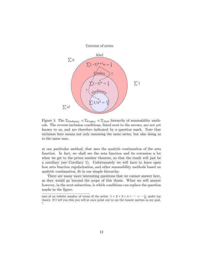
Where does this leave us? Figure 1 provides an overview of our currenthierarchy. Such figures provide good aid if we quickly want to formulatesome interesting questions. For example, we see that certain series are stillout of reach of even Abel summability. Which series are those? What sortof methods might sum them? And how can we relate these methods to ourcurrent hierarchy? Are they also stable and linear?

One of the series currently beyond our bounds is∑n, which plays a role

in theoretical physics (string theory). It turns out that we can reasonablysum it to −1/12. A rather counter-intuitive sum if we consider that weare adding only positive integers. Interestingly, the same summation canbe achieved by means of several very different techniques.4 We will look

4One of these techniques, that is of particular interest, is due to Ramanujan(1887–1920). In 1913, he writes to Hardy: “I was expecting a reply from you similarto the one which a Mathematics Professor at London wrote asking me to study carefullyBromwich’s Infinite Series and not fall pitfalls of divergent series. [...] I told him that the

11

Ordinary

Cesaro

Abel

∑1/n2 = π2

6

∑(−1)n = 1

2

∑(−1)n+1n = 1

4

∑n

∑1

∑n!

Universe of series

?

?

Figure 1: The ΣOrdinary ≺ ΣCesaro ≺ ΣAbel hierarchy of summability meth-ods. The reverse-inclusion conditions, listed next to the arrows, are not yetknown to us, and are therefore indicated by a question mark. Note thatinclusion here means not only summing the same series, but also doing soto the same sum.

at one particular method, that uses the analytic continuation of the zetafunction. In fact, we shall see the zeta function and its extension a lotwhen we get to the prime number theorem, so that the result will just bea corollary (see Corollary 1). Unfortunately we will have to leave openhow zeta function regularization, and other summability methods based onanalytic continuation, fit in our simple hierarchy.

There are many more interesting questions that we cannot answer here,as they would go beyond the scope of this thesis. What we will answerhowever, in the next subsection, is which conditions can replace the questionmarks in the figure.

sum of an infinite number of terms of the series: 1 + 2 + 3 + 4 + · · · = − 112

under mytheory. If I tell you this you will at once point out to me the lunatic asylum as my goal.”.

12

The theorems of Tauber and Hardy-Littlewood

Theorems that prove one summability method conserving another are calledAbelian theorems. A prime example is Theorem 1, which is indeed oftenreferred to simply as Abel’s theorem.5

Alfred Tauber proved in 1897 the first so-called Tauberian theorem.These theorems are the antonyms of Abelian theorems. They establishnontrivial conditions under which a weak summability method (usually theordinary) conserves a strong one, so that they are of equal strength whenthe conditions are satisfied.

It is not at all obvious that such Tauberian conditions can be formulatedfor any meaningful hierarchy of summability methods. Remarkably, Tauberestablished a simple sufficient condition for the Cesaro-Abel hierarchy ofFigure 1. For its proof, and the proofs of the other two (discrete) Tauberiantheorems we discuss, we follow [3], which in turn follows the elegant proofsof Karamata of 1930 [7].

To maintain a clear relation to the previous subsection, we will hereconsider only discrete Tauberian theorems, roughly those theorems thatinvolve summation instead of integration. The continuous Wiener-Ikeharatheorem is presented in the next section, where we also present a moredetailed comparison between the two types of Tauberian theorems, discreteand continuous.

Theorem 2 (Tauber, 1897). Under the Tauberian condition nan → 0, Abelsummability implies ordinary summability.

Proof. The proof is another example of the sort of series splitting argumentswe have seen earlier.

Define the number N(r) = b 11−rc, so that N(1− r) ≤ 1 and (N + 1)(1−

r) > 1. Because N → ∞ as r → 1−, and the limit limr→1−∑∞

n=0 anrn is

guaranteed to exist by assumption of Abel summability, it suffices to prove

limr→1−

( ∞∑n=0

anrn −

N∑n=0

an

)= 0 .

5Abel’s theorem might be familiar from real analysis. A common equivalent formula-tion is that the pointwise convergence of a power series on a set A implies the uniformconvergence of that power series on any compact subset K ⊂ A. (See for example theorem6.5.5 of [4].)

13

We split the series into

∞∑n=N+1

anrn −

N∑n=0

an(1− rn) .

By the Tauberian condition there exists for arbitrary ε > 0 a number N0

such that whenever n ≥ N0 we have the bound |nan| < ε. Pick δ > 0sufficiently small to satisfy N(r) ≥ N0 whenever 1 − δ < r < 1. With r(δ)close enough to 1, we can then bound the first term in the split as∣∣∣∣∣

∞∑n=N+1

anrn

∣∣∣∣∣ =

∣∣∣∣∣∞∑

n=N+1

nanrn

n

∣∣∣∣∣≤ ε

∞∑n=N+1

rn

n

≤ ε

N + 1

∞∑n=0

rn

=ε

(N + 1)(1− r)< ε .

For the second term, use again the Tauberian condition nan → 0, and recallobservation 1, to justify the bound 1

N

∑Nn=0 |nan| < ε for large enough N ,

and therefore∣∣∣∣∣N∑n=0

an(1− rn)

∣∣∣∣∣ =

∣∣∣∣∣N∑n=0

an(1− r)(1 + r + · · ·+ rn−1)

∣∣∣∣∣≤

N∑n=0

|nan|(1− r)

≤ Nε(1− r) < ε .

In 1914, Hardy and Littlewood established a similar minded result forgoing from Abel summability to Cesaro summability.

Theorem 3 (Hardy-Littlewood, 1914). Under the Tauberian condition sn ≥0, Abel summability implies Cesaro summability. In fact, it is sufficient toassume that sn ≥ −C for some positive constant C.

14

Proof. Assume the Abel sum∑anr

n → A as r → 1−. By equation (1), andsubstituting r with rk+1, then

∞∑n=0

sn(1− r)rn → A⇒∞∑n=0

sn(1− rk+1)rn(rn)k → A , (2)

for all k ≥ 0, as r → 1−. Noting that

limr→1−

1− rk+1

1− r= k + 1 = 1

/∫ 1

0tkdt ,

we can therefore write

(1− r)∞∑n=0

snrn(rn)k → A

∫ 1

0tkdt .

More general, by taking linear combinations, we see that for arbitrary poly-nomial P (t) similarly

(1− r)∞∑n=0

snrnP (rn)→ A

∫ 1

0P (t)dt . (3)

The Weierstrass approximation theorem tells us that for any piecewisecontinuous function g on [0, 1] and arbitrarily small ε > 0, there exist poly-nomials Pε(t) and Qε(t) such that Pε ≤ g ≤ Qε and ‖Qε − Pε‖ < ε. By (3)therefore

(1− r)∞∑n=0

snrnPε(r

n) ≥ −ε+A

∫ 1

0Pε(t)dt ≥ −2ε+A

∫ 1

0g(t)dt

and

(1− r)∞∑n=0

snrnQε(r

n) ≤ ε+A

∫ 1

0Qε(t)dt ≤ 2ε+A

∫ 1

0g(t)dt ,

if we take r close enough to 1. Now we use the Tauberian condition sn ≥ 0to obtain the sandwich

(1− r)∞∑n=0

snrnPε(r

n) ≤ (1− r)∞∑n=0

snrng(rn) ≤ (1− r)

∞∑n=0

snrnQε(r

n) ,

and consequently

(1− r)∞∑n=0

snrng(rn)→ A

∫ 1

0g(t)dt .

15

The left-hand side provides enough freedom to finish the proof, since thechoice of g is only subject to the fairly weak constraint of piecewise conti-nuity. In particular we need to look for piecewise continuous function g andnumbers rN such that rN → 1 as N →∞, and

rnNg(rnN ) =

1 if n ≤ N0 if n > N

.

We also need g to be normalized like∫ 1

0 g(t)dt = 1. The above conditionsuggests choosing g(t) = (1/t)χ[(rN )N , 1](t). By the normalization condition

we must then pick rN = e−1/N , which indeed matches the requirement thatrN → 1 as N → ∞. Furthermore, this choice implies g = (1/t)χ[1/e, 1], sothat we have g independent of N .

Given these choices we obtain

limN→∞

(1− rN )∞∑n=0

snrnNg(rnN ) = lim

N→∞(1− rN )

N∑n=0

sn = A .

But

limN→∞

N(1− rN ) = limN→∞

1− e−1/N

1/N= 1 ,

so we can introduce the partial Cesaro sums σN (see Definition 1) like

limN→∞

N(1− rN )1

N

N∑n=0

sn = limN→∞

σN = A ,

which is what we needed to prove.By the linearity of Abel and Cesaro summation, it suffices to assume

sn ≥ −C. Indeed, simply replace a0 with a0 +C and apply the theorem.

In 1911 Littlewood significantly weakened the Tauberian condition an =o(1/n) of the Tauber’s original theorem, demonstrating that it was by nomeans a necessity.6 The proof is very similar to that of Hardy-Littlewood,but requires some more technical detours.

Theorem 4 (Littlewood, 1911). Under the Tauberian condition an = O(1/n),Abel summability implies ordinary summability. In fact, it is sufficient toassume that nan > −C for some positive constant C.

6Weaker Tauberian conditions make for stronger Tauberian theorems. We thereforealso say, a bit counterintuitive, that we have improved the Tauberian conditions when wehave weakened them.

16

Proof. Assume the Abel sum∑anr

n → A as r → 1−. The proof is againby a sandwiching argument, but we need different polynomials to match thechanged objective. In particular we must get rid of the loose rn in (2). Thishas as a consequence that we are restricted to polynomials without constantterm.

By taking linear combinations, we have for any polynomial P (t) withP (0) = 0 that

∞∑n=0

anP (rn)→ AP (1) ,

as r → 1−. We also impose the normalizing constraint P (1) = 1.To circumvent these restrictions, we define P (t) in terms of a freely

chosen polynomial Q(t) by setting

P (t) = t+ t(1− t)Q(t) .

No matter what polynomial Q is chosen now, P has the imposed propertiesP (0) = 0 and P (1) = 1.

Similar as in the proof of Hardy-Littlewood, we take g(t) = χ[(rN )N , 1](t)

and rN = e−1/N ; so g = χ[1/e, 1]. To match Q(t), we define on [0, 1] thepiecewise continuous function

h(t) =g(t)− tt(1− t)

.

For arbitrary ε > 0 we then find Qε(t) such that h ≤ Qε and ‖Qε − h‖ < ε.Hence Pε(t) is such that g ≤ Pε and∫ 1

0

(Pε(t)− tt(1− t)

− g(t)− tt(1− t)

)dt =

∫ 1

0

(Pε(t)− g(t)

t(1− t)

)dt < ε , (4)

where we observe that any boundary issues are resolved by the integrabilityof∫ δ

0 1/t2 dt.As a result of the assumed normalization, we already have

limr→1−

∞∑n=0

anPε(rn) = A .

From this and the above bound, we would like to prepare the top slice ofthe sandwich, and show

lim supr→1−

∞∑n=0

ang(rn) ≤ A . (5)

17

Without loss of generality assume a0 = 0. By the Tauberian conditionand g ≤ Pε, we can bound

∞∑n=0

ang(rn)−∞∑n=0

anPε(rn) ≤ C

∞∑n=1

1

n(Pε(r

n)− g(rn))

≤ C∞∑n=1

1− r1− rn

(Pε(rn)− g(rn))

= C∞∑n=1

(rn − rn+1)Pε(r

n)− g(rn)

rn(1− rn).

The key insight to Karamata’s proof of Littlewood’s theorem, is that the lastbound can be interpreted as a Riemann sum of (4), with mesh size going to0 as r → 1−.7 So it follows that

lim supr→1−

∞∑n=0

ang(rn) ≤ limr→1−

∞∑n=0

anPε(rn)+C

∫ 1

0

(Pε(t)− g(t)

t(1− t)

)dt ≤ A+Cε ,

which gives (5) after squeezing the ε.Analogously we can show the other side of the sandwich

lim infr→1−

∞∑n=0

ang(rn) ≥ A .

Together with (5) this proves the theorem by the choice of g and rN , since

limN→∞

sN = limN→∞

∞∑n=0

ang(rn) = limr→1−

∞∑n=0

ang(rn) .

7Alternatively, sacrificing brevity, the nicer Darboux integral can be used. Begin bywriting ∣∣∣∣∣

∞∑n=1

(rn − rn+1)Pε(r

n)− g(rn)

rn(1− rn)−∫ 1

0

Pε(t)− g(t)

t(1− t) dt

∣∣∣∣∣≤∞∑n=1

∣∣∣∣∣Pε(rn)− g(rn)

rn(1− rn)(rn − rn+1)−

∫ rn

rn+1

Pε(t)− g(t)

t(1− t) dt

∣∣∣∣∣≤∞∑n=1

(sup

s, t∈[rn+1,rn]

∣∣∣∣Pε(s)− g(s)

s(1− s) − Pε(t)− g(t)

t(1− t)

∣∣∣∣)

(rn − rn+1) ,

then use uniform continuity, and the fact that the integrated function has only one jumpdiscontinuity.

18

The Wiener-Ikehara theorem

For the sake of completeness, we begin by stating some technical complexanalytic results (Theorem 5 and 6). Then we are ready to prove the centralresult of the thesis: the (weak) Wiener-Ikehara Tauberian theorem (The-orem 7). We do so in two steps. First we prove a Tauberian theorem forthe Laplace transform (Theorem 9), and then use that to prove a simplereformulation of Wiener-Ikehara (Theorem 8). For the proofs we follow thelecture notes of Siu [3].

Some complex analytic technicalities

The following basic results are used (tacitly) throughout the next subsection.They are technicalities, but form fundamental witnesses to the power andsuccess of complex analysis. Because we are interested in the prime numbertheorem, not a development of complex analysis, they are stated withoutproof.8

Theorem 5. The limit function f of a sequence of holomorphic functionsfn, is holomorphic in Ω, if the convergence is uniform in every compactsubset of Ω.

Theorem 6. Let f(z) be defined on the open set Ω ⊂ C in terms of aRiemann integral,

f(z) =

∫ 1

0F (z, t) dt .

Suppose that:

1. F (z, t) is holomorphic in z for each t.

2. F is continuous on Ω× [0, 1].

Then f(z) is holomorphic on Ω.

A proof of the Wiener-Ikehara theorem

The Tauberian result that will ultimately entail the prime number theorem(PNT) is given in Korevaar’s article [1] as

8The Cauchy-Goursat theorem and Cauchy’s integral formula are also assumed known.All mentioned statements can be found, with their proofs, in for example [2] (chapter 2).

19

Theorem 7 (The weak Wiener-Ikehara theorem). Suppose that the Dirich-let series

f(z) =

∞∑n=1

annz

,

with coefficients an ≥ 0, converges in the half plane z : Re z > 1; so thatthe summation function f(z) is automatically holomorphic in that half plane.Now also suppose that there exists a constant A such that the difference

g(z) = f(z)− A

z − 1

can be analytically continued to include the closure z : Re z ≥ 1 of thedomain of f(z). And finally assume that sn =

∑nk=1 an is in O(n). Then

sn/n→ A as n→∞, that is sn ∼ An.

In proving PNT, we will set an = Λ(n), where Λ(n) is the von Mangoldtfunction (Definition 5). The partial sum of this sequence is sn = ψ(n), thesecond Tchebychef function (Definition 6). It is straightforward to establishthe required bound ψ(n) ≤ Cn (Theorem 14).

With respect to the Tauberian condition, we show in the next sectionthat the Wiener-Ikehara theorem links ψ(n), through the choice of an, tothe Riemann zeta function ζ(z) (Definition 4) via the logarithmic derivativeas f(z) = −ζ ′(z)/ζ(z) (see Theorem 12). Crucially, we prove that ζ(z) hasa meromorphic continuation to the open right half plane z : Re z > 0(Theorem 10), and is nonzero on the critical line Re z = 1 (Theorem 11).The behavior of ζ(z) around the simple pole z = 1 will then allow us toconclude that g(z) can be analytically continued to the required half planeclosure, by setting A = 1.

Satisfying all conditions, we can apply the weak Wiener-Ikehara theoremto obtain ψ(n) ∼ n. Finally, a simple argument that is proved in the lastsection shows that PNT is equivalent to ψ(n) ∼ n (Theorem 15).

The difference with the original Wiener-Ikehara theorem, and the weak-ness in the above formulation, is that from the other assumptions alone,one can in fact deduce the supposition sn = O(n). Newman’s insight wasthat the full strength of the Wiener-Ikehara theorem is not needed to derivethe prime number theorem from it. Moreover, he recognized that a proofof this simplification could be accomplished with considerably less sophisti-cation. In particular, Newman was able to replace the used Wiener theorywith some clever contour integration, requiring nothing more than Cauchy’stheorem.

20

We now set out to prove Theorem 7. Recall Abel’s partial summationformula ∑

1≤n≤bxc

ana(n) = s(x)a(x)−∫ x

1s(t)a′(t)dt , (6)

where s(x) =∑

1≤n≤bxc an, and a(x) is assumed continuously differentiable.

Set a(x) = 1/xz, then a′(x) = −zx−z−1, and we see that it suffices to prove

Theorem 8. Let s(x), 1 ≤ x <∞, be a nonnegative, nondecreasing, piece-wise continuous function, such that s(x) ≤ Cx for some constant C. Define

f(z) = z

∫ ∞1

s(x)x−z−1dx ,

which is automatically holomorphic in half plane z : Re z > 1 becauses(x) = O(x). If g(z) = f(z)− A

z−1 can be analytically continued to an openneighborhood of the line Re z = 1, then s(x) ∼ Ax.

The advantage of this reformulation of the Wiener-Ikehara theorem, isthat its relation to the previously discussed discrete Tauber theory becomesmore explicit. That is, it is helpful in order to understand why we considerit a Tauberian theorem in the first place.

Recall from the previous section that “nowadays a Tauberian theoremmeans a statement which uses an appropriate Tauberian condition to guar-antee that a given way of taking weighted average (or weighted integral)gives the usual limit when the parameter in the given family of weightedaverage (or weighted integral) goes to an appropriate limit value”.

The proof of Theorem 8 will be a consequence of the following Laplacetransform Tauberian theorem.

Theorem 9 (Laplace transform Tauberian theorem). Let F (t), 0 ≤ t <∞,be a bounded, piecewise continuous function. If the Laplace transform of F ,

LF(z) =

∫ ∞0

F (t)e−ztdt ,

can be analytically continued to an open neighborhood U of the line Re z = 0,then limz→0 LF(z) = LF(0) =

∫∞0 F (t)dt.

Here, the family of weights used to average the content of the functionF (t) is e−zt, with a complex-valued family parameter z ∈ w : Rew > 0. Incontrast with the discussed discrete Tauber theory, we now weight “slices”of a continuous function, not elements of a sequence, and use an integral,

21

not a sum, to take the (function) content averages. Indeed, the function’scontent is indexed by the continuous interval 0 ≤ t <∞, and not the discreteinterval 0 ≤ n <∞.9

The deliberately general term “content” can be understood similarly asthe concept of norm. That is, a definition of size for a class of mathematicalobjects. The difference is that we do not insist on any (norm) axioms, andthat we are specifically concerned with families of weighted averages, eitherdiscretely or continuously indexed. Moreover, we have a particular interestin content definitions that involve sums or integrals. The goal of Taubertheory is to link these back to ordinary (common) assignments of content,such as the sum of elements for sequences (discrete case), or integration overan interval for piecewise continuous functions (continuous case).

In the above Tauberian theorem, the Tauberian condition is expressedas an assumption on the analytic horizon of the family of content assign-ments LF(z), namely that it can be analytically continued to an openneighborhood of the line Re z = 0. The conclusion is, as in the discrete case,that if we take the family parameter to an appropriate limit, here z → 0,the means converge to the ordinary definition of content, here

∫∞0 F (t)dt.

That is, limz→0 LF(z) =∫∞

0 F (t)dt.

Proof of Theorem 9. Let G(z) be the analytic continuation of LF(z) tothe open set U ⊃ z : Re z = 0, and define

Gλ(z) =

∫ λ

0F (t)e−ztdt .

By Theorem 6, Gλ(z) is entire. Also, by Theorem 5 and 6, and the bounded-ness assumption on F (t), G(z) is holomorphic in the closed right half plane.These are very strong properties, and allow us to proceed in the proof withrelative ease.

It suffices to prove that G(0) − Gλ(0) → 0 as λ → ∞. Because of theTauberian condition, we can use Cauchy’s integral formula to convenientlyrephrase this problem in terms of a contour integral. Generally we prefer towork with such integrals, because we have a lot of nice standard tools fromcomplex analysis to handle them. Hence we write

G(0)−Gλ(0) =1

2πi

∫C

(G(z)−Gλ(z)

z

)dz .

9Compare the definition of Abel summability in Definition 3. Siu in [3] gives a tabulatedcomparison to Tauber’s original theorem, which is quite useful.

22

The theorem will follow from an appropriate choice of contour C, and partialestimation of the Cauchy integral.

Pick ε > 0 arbitrarily. For x = Re z > 0, we have

G(z)−Gλ(z) =

∫ ∞λ

F (t)e−ztdt , (7)

and bound

|G(z)−Gλ(z)| ≤ e−λx

x=

∣∣e−λz∣∣Re z

. (8)

To neutralize the problematic denominator Re z, which might blow up onC, we note for |z| = R that

1

z+

z

R2=

2Re z

R2, (9)

Now the crux of the proof. We replace the usual 1/z kernel of Cauchy’sintegral formula with eλz(1/z + z/R2). This new kernel is likewise mero-morphic on C, and has a simple pole at z = 0 of residue 1.10 The additionalterms are key in obtaining the desired estimates. The reason is that for ourchoice of contour C in Cauchy’s formula, both Re z > 0 and Re z < 0 occur.In the latter case, (8) might be problematic.

So we must show that∣∣∣∣∫C

(G(z)−Gλ(z))eλz(

1

z+

z

R2

)dz

∣∣∣∣ < ε , (10)

for some valid contour C.11 Let δR > 0 be a function of R, chosen so that|z| ≤ R : Re z ≥ −δR ⊂ U . We cut CR,δR := C up into three parts, andshow (10) for each part individually. As depicted in Figure 2, the chosensegments are: the right half circle

C+R = |z| = R : Re z > 0 ,

the union of two (small) circle arcs in the left half plane

AR,δR = |z| = R : −δR < Re z < 0 ,

and the vertical line segment connecting those arcs

LR,δR = |z| < R : Re z = −δR .

10A quick review of the proof of Cauchy’s integral formula shows that this replacementof the kernel is indeed allowed here. Note that ((G(z) − Gλ(z)) − (G(0) − Gλ(0)))/z isbounded because G(z)−Gλ(z) is holomorphic, and that z/R2 = (z2/R2)/z.

11Piecewise smooth is good enough. See [2], appendix B.

23

x

iy

RδR

AR,δR

AR,δR

LR,δR

C+R

Figure 2: The integration contour for the Laplace transform Tauberian the-orem. The contour is split into the three marked segments C+

R , AR,δR , andLR,δR .

24

We start with C+R . From (8) and (9) it immediately follows that∣∣∣∣(G(z)−Gλ(z))eλz

(1

z+

z

R2

)∣∣∣∣ ≤∣∣e−λz∣∣Re z

∣∣∣eλz∣∣∣ 2Re z

R2=

2

R2,

and therefore∣∣∣∣∣∫C+R

(G(z)−Gλ(z))eλz(

1

z+

z

R2

)dz

∣∣∣∣∣ ≤ πR 2

R2< ε/3 ,

if R is chosen large enough. The somewhat mysterious choice for the non-standard Cauchy kernel eλz(1/z+z/R2) should begin to appear less opaquenow.

In the left half plane we can no longer make use of (7), so for AR,δR∪LR,δRwe treat G(z) and Gλ(z) separately. Their (assumed) analytical propertieswill provide the required bounds.

Since Gλ(z) is entire, by the Cauchy–Goursat theorem, we may replacethe contour AR,δR ∪ LR,δR with |z| = R : Re z < 0. Similarly to thesituation above, but now for x = Re z < 0, we have the bound

|Gλ(z)| ≤ e−λx

−x=

∣∣e−λz∣∣−Re z

,

and therefore∣∣∣∣∣∫|z|=R:Re z<0

Gλ(z)eλz(

1

z+

z

R2

)dz

∣∣∣∣∣ ≤ πR 2

R2< ε/3 ,

if R is chosen large enough. Notice that the change of contours is necessi-tated by the condition |z| = R required to apply (7).

For G(z) we treat AR,δR and LR,δR separately. Fix R large enough, thenpicking δR > 0 small, we immediately establish the bound < ε/6 for AR,δR .Finally, remember that even if R and δR are fixed, we still have the freedomto choose λ as big as we wish, and so for the LR,δR contour∣∣∣∣∣

∫LR,δR

G(z)eλz(

1

z+

z

R2

)dz

∣∣∣∣∣ ≤ Ce−λδR < ε/6 .

We now finish the proof of the Wiener-Ikehara theorem by proving The-orem 8 (repeated here for convenience).

25

Theorem. Let s(x), 1 ≤ x <∞, be a nonnegative, nondecreasing, piecewisecontinuous function, such that s(x) ≤ Cx, for some constant C. Define

f(z) = z

∫ ∞1

s(x)x−z−1dx ,

which is automatically holomorphic in half plane z : Re z > 1, becauses(x) = O(x). If g(z) = f(z)− A

z−1 can be analytically continued to an openneighborhood of the line Re z = 1, then s(x) ∼ Ax.

Proof. Let F (t) = e−ts(et) − A. Under the theorem’s conditions, F isbounded and piecewise continuous on 0 ≤ t < ∞. We may therefore takeits Laplace transform G(z) = LF(z). For G we have

G(z) =

∫ ∞0

F (t)e−zt dt

=

∫ ∞0

(e−ts(et)−A

)e−zt dt

=

∫ ∞1

(1

xs(x)−A

)x−z

1

xdx

=1

z + 1(z + 1)

∫ ∞1

s(x)x−(z+1)−1 dx− A

z

=1

z + 1

(f(z + 1)− A

z−A

),

and so by the assumptions on g(z) = f(z)− Az−1 , we can apply the Laplace

transform Tauberian theorem (Theorem 9) to it. In fact, this is the wholepoint of our curious choice of F (z).

Now∫∞

0 F (t) dt exists, and therefore∫ ∞1

(s(x)

x−A

)1

xdx =

∫ ∞0

(e−ts(et)−A) dt =

∫ ∞0

F (t) dt (11)

also exists, and by definition is finite. This strongly suggests using thefollowing proof technique.

Suppose we could show that for any ε > 0, there exists a constant X suchthat whenever x0 ≥ X, we have s(x0)/x0 − A ≤ ε and s(x0)/x0 − A ≥ −ε.That would establish the theorem. Using this observation, we proceed with aproof by contradiction; so assume that for some ε > 0, there exists a sequencexn, xn → ∞, such that s(xn)/xn − A > ε. We would like to contradictthis with the finiteness of (11). The method for proving s(x0)/x0 −A ≥ −εwhen x0 ≥ X is entirely analogous.

26

Recall that s(x) was assumed to be nonnegative and nondecreasing.Hence, if s(xn)/xn − A > ε, it should hold that s(xn)/xn − A > ε/2 forsome interval up ahead. We may pick this interval conveniently as

Ixn,ε =

[xn,

A+ ε

A+ ε2

xn

]⊂ [xn,∞) .

Indeed, for x ∈ Ixn,ε we see that per assumption s(x) ≥ s(xn) > xn(A+ ε),and so

s(x)/x−A >xn(A+ ε)

xn

(A+εA+ε/2

) −A =ε

2.

We then compute∫Ixn,ε

(s(x)

x−A

)1

xdx >

ε

2

∫ A+εA+ε/2

xn

xn

1

xdx =

ε

2log

(A+ ε

A+ ε2

)> 0 ,

which is independent of xn. But by the proof by contradiction assumption,there are infinitely many such xn. Moreover, their respective intervals Ixn,εneed not necessarily overlap, as we choose xn → ∞. So we have arrived ata statement contradicting the finiteness of (11).

27

The Riemann zeta function

We need two results on the Riemann zeta function ζ(z) (Definition 4) touse it in applying (Korevaar’s version of) the Wiener-Ikehara Tauberiantheorem to the proof of PNT. Additionally, we must show that f(z) =∑

n Λ(n)/nz = −ζ ′(z)/ζ(z) (Theorem 12), to establish the link between thezeta function and the Tauberian condition needed to derive ψ(x) ∼ x, andso PNT. Here Λ(n) is the von Mangoldt function (Definition 5); ψ(x) is thesecond Tchebychef function (Definition 6).

The first result we need on the zeta function is its meromorphic continu-ation to the open right half plane (Theorem 10). The second required resultbuilds on the first, and says that ζ(z) is nonzero on the line Re z = 1 (Theo-rem 11). Through the above linking formula, these theorems together thenquickly prove the necessary meromorphic continuation of f(z) to an openneighborhood of the line Re z = 1 (Theorem 12), and so with ψ(x) = O(x)prove ψ(x) ∼ x. The proofs are taken mainly from [2] and [3], but areentirely standard.

The meromorphic continuation of the zeta function

Already from the discussion in the previous section, the importance of thezeta function for number theory is manifest. Euler (1707-1783) first usedit to show that the sum

∑1/p diverges; presenting the first quantitative

statement on the number of primes since Euclid. Later, in 1859, Riemannintroduced the idea of applying complex analytic techniques, via Euler’s zetafunction, to the analysis of the prime counting function π(x) (Definition 7);he also initiated the still ongoing investigation into the distribution of thezeros of the zeta function.12 Knowledge of this distribution has provenpivotal to the application of the Riemann zeta function to number theory.In particular, to prove the prime number theorem, we shall need that ζ(z)is nonzero on the line Re z = 1. In the previous section we observed thecritical nature of this line for the Tauberian condition of the Wiener-Ikeharatheorem.

Definition 4. The (Euler) zeta function is initially defined on the half plane

12The classical reference is Riemann’s 1859 paper “Uber die Anzahl der Primzahlenunter einer gegebenen Grosse”. Here Riemann stated arguably the most famous openproblem in of all of mathematics, the Riemann hypothesis; and introduced the now stan-dard “zeta notation” ζ(z) :=

∑1/nz.

28

z : Re z > 1 as

ζ(z) =

∞∑n=1

1

nz,

where it is automatically holomorphic.

Riemann’s major contribution was in his proof of the existence of ameromorphic continuation of Euler’s zeta function to the entire complexplane. Identifying a single simple pole at z = 1 of residue 1. This extendedzeta function we call the Riemann zeta function.

To apply Theorem 7, we only need the meromorphic continuation of−ζ ′(z)/ζ(z) to some open set containing the line Re z = 1; so we can getaway with a bit less than Riemann’s result.13 Namely a continuation upto the line Re z = 0, which easily follows from Abel’s partial summationformula (see next theorem).

Remember however that no matter what methods we choose to pursuethe meromorphic continuation of the zeta function, we cannot arrive at dif-ferent definitions of ζ(z) in the domain so extended (the identity theorem).Hence the use of the definite article “the” in “the meromorphic continua-tion” is warranted. In particular, we shall look at two different extensionapproaches (with a third given in the appendixes).

Theorem 10. The zeta function can be meromorphically continued to theopen right half plane, with a single simple pole at z = 1 of residue 1. Forthe extended function we have the explicit formula

ζ(z) =1

z − 1+ 1− z

∫ ∞1tt−z−1 dt ,

where t = t− btc is the fractional part function.

Proof. By Abel’s partial summation formula (6), taking an = 1 and a(x) =1/xz, for Re z > 1 we may write

ζ(z) = z

∫ ∞1btc t−z−1 dt .

Now notice that the problematic extra order of growth in the integrand,contributed by the integral part function btc, can be canceled by rewriting

z

∫ ∞1btc t−z−1 dt = z

∫ ∞1

(btc − t)t−z−1 dt+ z

∫ ∞1

t−z dt ,

13Recall that complex differentiable functions are automatically infinitely complex dif-ferentiable. See [2], chapter 2 for reference.

29

so that

ζ(z) =1

z − 1+ 1− z

∫ ∞1tt−z−1 dt .

This method can be extended to yield meromorphic continuations to thesets z : Re z > −m, for any m ∈ N; and hence to the entire complex plane.Define Q0(x) = x − 1/2, then

ζ(z) =z

z − 1− 1

2− z

∫ ∞1

Q0(x)

xz+1dx .

We continue to recursively define Qk(x) by imposing the three properties

1. ddxQk+1 = Qk

2. Qk(x+ 1) = Qk(x)

3.∫ 1

0 Qk(x) dx = 0 .

These polynomials are related to the Bernoulli polynomials on 0 ≤ x ≤ 1by the equation

Qk(x) =Bk+1(x)

(k + 1)!.

In turn, Bernoulli numbers Bk arise as special values of these polynomials,namely Bk = Bk(0). The first few Bernoulli numbers are B1 = −1/2,B2 = 1/6, B3 = 0, B4 = −1/30.

With property 1, rewrite

ζ(z) =z

z − 1− 1

2− z

∫ ∞1

(dk

dxkQk(x)

)1

xz+1dx .

Integration by parts then extends the meromorphic continuation of ζ(z) intoz : Re z > −k − 1.

Specifically, we have

ζ(z) =z

z − 1− 1

2− z

Q1(x)

xz+1

∣∣∣∣∞1

− z(z + 1)

∫ ∞1

Q1(x)

xz+2dx

ζ(z) =z

z − 1− 1

2+ z

B2

2− z(z + 1)E(z) .

Now using the above properties 2 and 3, we can apply Dirichlet’s test tothe integral E(z). Therefore, by Theorem 5 and 6, we see that E(z) is

30

holomorphic in the half plane Re z > −2. Repeated application of thesesteps yields the general extension.

We are now also able to sum∑n = −1/12. If we symbolically extend

Euler’s zeta function, and associate it with Riemann’s analytic continua-tion, we can imagine that ζ(−1) =

∑ 1n−1 . In this spirit, zeta function

regularization acts as a summability method. In particular, we have

Corollary 1. Zeta function regularization assigns the sums

∞∑n=1

nk = ζ(−k) = −Bk+1

k + 1,

for nonnegative integers k. Specifically,∑

1 = −1/2 and∑n = −1/12.

Another approach to the meromorphic continuation of ζ(z) is to startwith the gamma function Γ(z), initially defined for s > 0 as

Γ(z) =

∫ ∞0

e−ttz−1 dt .

It can be shown that 1/Γ(z) admits an analytic continuation to the entirecomplex plane14.

By Fubini-Tonelli theorem, since 1/(ex−1) =∑e−nx, we may swap the

integral and sum, and write

ζ(z) =1

Γ(z)

∫ ∞0

xz−1

ex − 1dx ,

for Re z > 1. Splitting the integral, we therefore obtain

ζ(z) =1

Γ(z)

∫ 1

0

xz−1

ex − 1dx+ E(z) ,

with E(z) entire.Recall the generating function of the Bernoulli numbers (commonly taken

as definition) as

x

ex − 1=

∞∑n=0

Bnn!xn .

Using Fubini-Tonelli again then yields∫ ∞0

xz−1

ex − 1dx =

∞∑n=0

Bnn!(z + n− 1)

.

14See for example [2], chapter 6, pp. 160-168; and in particular, theorem 1.6, p. 165.

31

The right hand side is entire, except for poles at z = 1, 0,−1, · · · . However,leaving z = 1, these are all canceled by the zeros of 1/Γ(z). So by theidentity theorem, we are done.

The zeta function is nonzero on the line Re z = 1

The following truly inspired proof is due to F. Mertens (1840–1927). Ittremendously simplifies a considerable hurdle in the early proofs of the primenumber theorem. The details are taken from [2], chapter 7.

Theorem 11. The Riemann zeta function does not vanish on the lineRe z = 1.

Proof. At the heart of Mertens’s proof is the trigonometric identity

3 + 4 cos θ + cos 2θ = 3 + 4 cos θ + 2 cos2 θ − 1 = 2(1 + cos θ)2 ≥ 0 ,

and the auxiliary function h(x), defined for x > 1 as

h(x) = ζ(x)3ζ(x+ iy)4ζ(x+ 2iy) .

Recall Euler’s product formula for his zeta function

ζ(z) =∏

p prime

1

1− p−z,

which is valid in the plane U = z : Re z > 1. An important corollary isthat ζ(z) has no zeros in U , and so log ζ(z) is holomorphic there (see [2],chapter 3, Theorems 5.2 and 6.2; chapter 5, proposition 3.1; chapter 7, pp.182-184).

We can conveniently use product formulas to absorb logarithms. For the

32

zeta function

log ζ(z) = log∏

p prime

1

1− p−z

=∑

p prime

log

(1

1− p−z

)

=∑

p prime

∞∑n=1

p−nz

n

=∑p,m

p−mz

m

=∞∑n=1

cnnz

,

(12)

where cn = 1/m ≥ 0 if n = pm, and zero otherwise. Recall here the analyticcontinuation of the power series expansion of the real logarithm

log

(1

1− x

)=∞∑n=1

xn

n.

Also, in the last steps we may indeed safely ignore the order of summation(up to a bijection), because the double series converges absolutely (see [2],chapter 7, pp. 197-199).

Set z = x+iy; verify that log |z| = Re log z, and Re(n−z) = n−x cos(y log n).As a result of the trigonometric identity above, we can then bound the log-arithm of Mertens’s auxiliary function from below by

log |h(x)| = 3 log |ζ(x)|+ 4 log |ζ(x+ iy)|+ log |ζ(x+ 2iy)|

=

∞∑n=1

cnn−x(3 + 4 cos θn + cos 2θn)

≥ 0 ,

where θn = y log n. Hence |h(x)| ≥ 1. Using this bound we give a proof bycontradiction.

Suppose contrary to the theorem that ζ(z0) = 0 at some point z0 =1 + iy0 6= 1 on the line Re z = 1. We know that the extended zeta functionis per definition holomorphic at this z0; therefore if we approach along thehorizontal line x+ iy0, we have the bound

|ζ(x+ iy0)− ζ(z0)| = |ζ ′(z0)||x− 1|+ o(x− 1) ,

33

and hence for C > 0 constant

|ζ(x+ iy0)| ≤ C|x− 1|⇒ |ζ(x+ iy0)|4 ≤ C|x− 1|4 .

Similarly, at the pole we find

|ζ(x)|3 ≤ C ′|x− 1|−3 .

We now observe that in bounding h(x), the small terms |x−1| overpowerthe large terms 1/|x− 1|. So we have

|h(x)| = |ζ(x)|3 |ζ(x+ iy)|4 |ζ(x+ 2iy)| ≤ C ′′(x− 1) .

Taking then x → 1+ (recall that h(x) is only defined for x > 1), we arriveat the sought after contradiction.

Combining Theorem 10 and 11, it is straight forward to prove the resultwe need to apply the Wiener-Ikehara theorem to the proof of PNT via thezeta function (Theorem 12). But before we continue, we require one moretechnical lemma. Also, we now explicitly need the two auxiliary functionsΛ(n) and ψ(x) we mentioned several times earlier. First the lemma.15

Lemma 1. Suppose Fn is a sequence of functions, holomorphic on theopen set Ω ⊂ C. If there exist constants cn > 0 such that

∑cn < ∞, and

|Fn(z)− 1| < cn for all z ∈ Ω, then

1. The product∏Fn(z) converges uniformly in Ω to a holomorphic func-

tion F (z).

2. If Fn(z) does not vanish for any n,

F ′(z)

F (z)=

∞∑n=1

F ′n(z)

Fn(z).

The following two number theoretic auxiliary functions pop up frequentlywhen analyzing the prime counting function π(x) (Definition 7). Studyingthe relations between such arithmetical functions is key in number theory.The associated Greek letters are standard notation (similarly to the use ofzeta for Riemann’s function).

15For a proof refer to [2], chapter 5, proposition 3.2 (pp. 141-142).

34

Definition 5. The von Mangoldt function Λ(n) is defined on the naturalnumbers as

Λ(n) =

log p if n = pk for prime p

0 otherwise.

Definition 6. The (second) Tchebychef function ψ(x) is the summation ofthe von Mangoldt function up to x (as in Abel’s formula). That is,

ψ(x) =∑

1≤n≤bxc

Λ(n) .

We now return to the discussion about the role of the Wiener-IkeharaTauberian theorem in proving the prime number theorem (refer to directly

below Theorem 7). Recall that we there set f(z) =∑

nΛ(n)nz . We establish

the link between the zeta function and the Tauberian condition needed toderive ψ(x) ∼ x (and so PNT) through the formula f(z) = −ζ ′(z)/ζ(z); andsubsequently can prove the meromorphic continuation of f(z) to an openneighborhood of the line Re z = 1, as required by the condition. This shouldclarify the interplay between the Tchebychef ψ-function, the Riemann zetafunction, the Wiener-Ikehara Tauberian theorem, and the prime numbertheorem.

In the next section we then finally show ψ(x) = O(x), and prove theequivalence of PNT and ψ(x) ∼ x. Thereby finishing the argument.

Theorem 12. Define

f(z) =

∞∑n=1

Λ(n)

nz,

if Re z > 1, then

f(z) = −ζ′(z)

ζ(z). (13)

Furthermore, f(z) admits a meromorphic continuation to an open neighbor-hood of the line Re z = 1. Moreover, like ζ(z), f(z) has as only singularitya simple pole at z = 1 of residue 1.

Proof. Applying the above Lemma 1 to the Euler product formula, we obtain

−ζ′(z)

ζ(z)=

∑p prime

p−z log p

1− p−z=

∑p prime

∞∑n=1

log p

(pn)z=∞∑n=1

Λ(n)

nz.

Here the series rearrangement in the last step is allowed, because the doublesum converges absolutely (compare the derivation of (12) in Theorem 11).

35

As a result of this formula, the meromorphic continuation of f(z) fol-lows from extending the logarithmic derivative −ζ ′(z)/ζ(z). The problem ishowever, that 1/ζ(z) might not be defined. So we need to use our knowledgeof the distribution of the zeros of the Riemann zeta function.

We observed earlier (in proof of Theorem 11) that the Euler productformula implies that ζ(z) is nonzero on the half plane z : Re z > 1.The demonstrated properties of the Riemann zeta function (Theorem 10and 11) extend this non-vanishing result to an open set U containing thecritical line Re z = 1. On U the reciprocal 1/ζ(z) exists, and is holomorphic.Consequently, f(z) admits a meromorphic continuation to U , and thereforeto a neighborhood of the line Re z = 1.

Finally, from (13) and the product rule for differentiation, we immedi-ately see that f(z), like ζ(z), has as only singularity a simple pole of residue1 at z = 1.

36

The prime number theorem

We define yet another auxiliary arithmetical function.

Definition 7. The prime counting function π(x) denotes the number ofprimes up to and including x.

The prime number theorem (PNT) now reads

Theorem 13 (Hadamard, de La Vallee Poussin, 1896). As x→∞, primesdistribute like

π(x) ∼ x

log x.

We are left to show the linear bound ψ(x) ≤ Cx, for some constant C(Theorem 14), and relate Tchebychef’s ψ-function to PNT (Theorem 15).The proofs are entirely standard.

The linear bound on the Tchebychef ψ-function

Theorem 14. The second Tchebychef function ψ(x) is linearly bounded.That is, ψ(x) = O(x).

Proof. We can relate the product of primes in the interval (n, 2n] to thebinomial coefficient

(2nn

)through the inequality

∏n<p≤2np prime

p ≤ (n+ 1)(n+ 2) · · · (2n)

1 · 2 · · ·n=

(2n

n

).

Binomial coefficient are easier to manipulate and estimate than products ofprimes. In particular, we can immediately see that

(2nn

)< 22n. Therefore

by taking logarithms, we establish the crude bound∑n<p≤2np prime

log p < 2n log 2 .

Now assume n = 2m. We can then divide (1, n] into subintervals (2l, 2l+1],for l ∈ [0,m− 1], to obtain∑

p≤2m

p prime

log p < 2m+1 log 2 . (14)

37

Recall the definition of the Tchebychef’s ψ-function (Definition 6). Wesee immediately that we can rewrite it to

ψ(x) =∑

p prime

⌊log x

log p

⌋log p .

The key idea of the proof is to differentiate relative to x between “small”and “big” primes, and accordingly split the above formula. We can thenlinearly bound both parts separately.

We say that p is a small prime relative to x if p2 ≤ x. Otherwise we sayit is a big prime (relative to x). These cases correspond to blog x/ log pc > 1and blog x/ log pc = 1 respectively. For the small primes p ≤

√x, and

therefore ∑p small

⌊log x

log p

⌋log p ≤

∑p≤√x

⌊log x

log p

⌋log p

≤∑p≤√x

log x

= π(√x) log x .

Where we take to our advantage, the ability to introduce the square root inthe term π(

√x). For the big primes, take m such that 2m ≤ x ≤ 2m+1; then

by equation (14) we may bound∑p big

⌊log x

log p

⌋log p =

∑p big

log p

≤ 2m+2 log 2 ≤ 4x log 2 .

Here the advantage is the “cheap” disposal of the term blog x/ log pc.Now notice that π(x) ≤ x. The two bounded pieces of ψ(x) taken

together then yield the result

ψ(x) ≤ π(√x) log x+ 4x log 2

≤√x log x+ 4x log 2

=

(log x√x

+ 4 log 2

)x

= O(x) .

38

Equivalent formulations of PNT

By Theorem 12 and 14, we can apply the Wiener-Ikehara theorem withA = 1 to an = Λ(n), and conclude that ψ(x) ∼ x. Hence the prime numbertheorem is a corollary of

Theorem 15. If ψ(x) ∼ x, then π(x) ∼ x/ log x, for x→∞.

Proof. Under the assumption ψ(x) ∼ x, it suffices to prove ψ(x) ∼ π(x) log x.We do so by the standard sandwiching technique of bounding with the samenumber, the limsup from above, and the liminf from below (as in the proofof Littlewood’s 1911 Theorem 4). We see the limsup bound at once, but theliminf bound is more difficult. We again need to split the problem.

Note that 1 ≤ lim inf ψ(x)/(π(x) log x) iff lim sup (π(x) log x)/ψ(x) ≤1, so that we may also prove the latter inequality. Choose yx < x, andseparately consider the primes p ≤ yx, and the primes yx < p ≤ x, to obtain

π(x) =∑p≤yx

1 +∑

yx<p≤x1

= π(yx) +1

log yx

∑yx<p≤x

log p

≤ yx +ψ(x)

log yx.

Rewriting yieldsπ(x) log x

ψ(x)≤ yx log x

ψ(x)+

log x

log yx.

So since ψ(x) ∼ x, we can conveniently swap ψ(x) for x, and it suffices topick yx such that

lim supx→∞

log x

log yx≤ 1 ,

and

lim supx→∞

yx log x

x≤ 0 .

A good choice is

yx =x

(log x)2.

39

One reason to be interested in PNT is its use in understanding the struc-ture of the prime number sequence pn. Indeed, pn appears to behave quiterandomly; and it is not even easy to provide an approximating sequence.Using the prime number theorem however, we can establish such an (asymp-totic) estimate. In fact, the estimate and PNT are equivalent.16

Theorem 16. The prime number theorem is equivalent to the asymptoticestimate

pn ∼ n log n as n→∞ .

Proof. (⇒) First note that π(pn) = n; then in the PNT estimate set x = pnto get pn ∼ n log pn. Thus we need to show log pn ∼ log n. Take logarithmsand use continuity to obtain

log n

log pn+

log log pnlog pn

− 1→ 0 .

The middle term vanishes, hence by definition pn ∼ n log n.(⇐) Let pn ≤ x < pn+1, then

pnn log n

≤ x

π(x) log π(x)<

pn+1

n log n,

and therefore x ∼ π(x) log π(x). Analogous to how we established log pn ∼log n, we can now prove log π(x) ∼ log x. Hence π(x) ∼ x/ log x.

As a final observation we note that PNT can be understood “proba-bilistically”, despite that being prime is not a probabilistic concept. Theasymptotic estimate suggests using the heuristic Prob(n prime) = 1/ log n;the expected number of primes under x is then given by∑

2≤n≤xP(n prime) =

∑2≤n≤x

1

log n.

This approximation is numerically far superior to x/ log x (see also [5]). Infact, for the closely related (offset) logarithmic integral function

Li(x) =

∫ x

2

1

log tdt ,

we have the following precise theorem due to H. von Koch (1870-1924).

16In the sense that there are quick proofs of PNT ⇒ estimate, and estimate ⇒ PNT.Similarly we can say that ψ(x) ∼ x and PNT are equivalent. Theorem 15 proves one sideof this statement.

40

Theorem 17 (von Koch, 1901). The Riemann zeta function has no zerosin the strip α < Re z < 1 if and only if

π(x)− Li(x) = O(xα+ε) as x→∞

for every ε > 0 (and fixed 1/2 ≤ α < 1).

The theorem links the distribution of the zeros of ζ(z), through theRiemann hypothesis, to the estimation of the prime counting function. Thisillustrates once again the importance of the locations of the zeta functionzeros for number theory.17

It should not surprise the reader that

Theorem 18. The (offset) logarithmic integral function has the asymptoticestimate

Li(x) ∼ x

log x.

So PNT is equivalent to π(x) ∼ Li(x).

Proof. Partial integration yields∫ x

2

1

log tdt =

x

log x− 2

log 2+

∫ x

2

1

(log t)2dt .

So we are done if we can prove that the last integral is of order o(x/ log x).A clever split of the integration domain suffices:∫ x

2

1

(log t)2dt =

(∫ √x2

+

∫ x

√x

)1

(log t)2dt

≤ C√x+ C ′

x−√x

(log√x)2

≤ C x

(log x)2.

17The Riemann hypothesis proposes that ζ(z) = 0 ⇒ Re z = 1/2. I am not sure howmuch credit von Koch deserves for the theorem. Whether he simply first stated it, proveda weaker version, or showed just one implication, I don’t know.

41

Appendix A: the prime polynomial theorem

It is instructive to see how the zeta function, along with the various familiarauxiliary functions, come up in the proof of the polynomial version of PNT.18

Interestingly, the bounds provided by this prime polynomial theorem (PPT)satisfy a von Koch type condition (refer to Theorem 17), or a “Riemannhypothesis” for polynomials.

We first revisit the Riemann zeta function and the auxiliary arithmeticalfunctions of the PNT proof, and define polynomial variants. We use thestandard notation Fq to denote a finite field of order q. Similarly we useFq[x] to mean the ring of polynomials over Fq.

Take the degree of a polynomial as norm. The ring Fq[x] is then Eu-clidean in the sense that Euclid’s algorithm is valid. Consequently, we canestablish an analogue of Bezout’s lemma, and therefore it makes sense totalk about irreducibles (polynomials without nontrivial factors) as primes.Being prime is understood here in the sense of Euclid’s lemma. That is, Pis prime if and only if P |AB ⇒ P |A or P |B. From now on we treat theterms “irreducible” and “prime” as synonyms.

In fact, like the natural numbers, Fq[x] is a unique factorization domain.Meaning that a version of the fundamental theorem of arithmetic holds.In particular, every polynomial in Fq[x] has a unique representation as aproduct of irreducibles, up to order and multiplication by scalars.

Definition 8. The polynomial prime counting function πq(n) gives the num-ber of monic irreducible polynomials in Fq[x] of degree n.

Definition 9. The polynomial von Mangoldt function is given by

Λ(f) =

degP if f = P k a power of a prime P

0 otherwise.

Definition 10. The polynomial Tchebychef ψ-function is defined using thevon Mangoldt function as the finite sum

ψ(n) =∑

deg f=nf monic

Λ(f) . (15)

18More proofs of polynomial equivalents of (famous) number theoretic theorems canbe found in the bachelor thesis [8]. In particular, the thesis discusses several other (ele-mentary) proofs of the polynomial version of PNT, as well as equivalents for Dirichlet’stheorem and the notion of Tchebychef bias.

42

Definition 11. The polynomial zeta function ζq(z) is initially defined onz : Re z > 1 as

ζq(z) =∑

0 6=f∈Fq [x]f monic

1

|f |z. (16)

Here |f | = qdeg f . That is, the norm of f is the number of distinct polyno-mials in Fq[x] of degree less than deg f .

Note that in the definition of the zeta function ζq(s), we rely on theabsolute convergence of the series to be able to ignore the precise order ofsummation (recall Riemann’s rearrangement theorem). We will continue toassociate |f | = qdeg f .

We formulate PPT in probabilistic terms, as we did earlier for PNT.This has as advantage that it makes the statement appear more intriguing,and therefore easier to remember.

Theorem 19 (PPT). A random polynomial in Fq[x] of degree n has theasymptotic probability 1/n to be irreducible. More precisely

πq(n) =qn

n+O

(√qn

n

). (17)

Writing x = qn, this resembles the prime number theorem:

πq(n) ∼ x/ logq(x) .

We can also formulate an Euler product for ζq(z). Its proof is analogousto proof of the usual Euler product, except for some technicalities. It islikewise a codification of the fundamental theorem of arithmetic (for Fq[x]).

Note that for monic polynomials P and Q, conveniently |PQ| = |P ||Q|.

Theorem 20 (Euler product). For Re z > 1, we have

ζq(z) =∏

P primeand monic

1

1− |P |−z,

where the product is taken from small to large polynomial degree.

A nice corollary is the polynomial variant of Euler’s classical zeta func-tion application.

43

Corollary 2. There are infinitely many monic irreducible polynomials. Infact, we have the stronger divergence result∑

P irreducibleand monic

1

|P |→ ∞ . (18)

Very different from the regular zeta function however, is the simplicityof the meromorphic continuation of ζq(z).

Theorem 21. The zeta function has a meromorphic continuation to theentire complex plane given by

ζq(s) =1

1− q1−z .

Proof. Assume Re z > 1. A simple series rearrangement gives

∑0 6=f∈Fq [x]f monic

1

|f |z=∞∑n=0

∑deg f=nf monic

1

|f |z

=

∞∑n=0

1

qnzqn

=∞∑n=0

(q1−z)n .

By working backwards, this also immediately provides the required absoluteconvergence. Note here the convenient choice of | · |.

The geometric series formula yields the stated meromorphic continua-tion, with poles at s = 1 + i 2π

log qn, for n ∈ N.

We now prove an explicit formula for the (polynomial) Tchebychef ψ-function, reminiscent of the asymptotic formula ψ(x) ∼ x.19 Using some

19Explicit formulas also exist for the usual Tchebychef ψ-function (and for other arith-metical functions), but they are more involved, and harder to prove. Such number theo-retic formulas were initially investigated by Riemann in relation to the distribution of theprimes, beginning with his seminal 1859 paper. In fact, the explicit formula∫ x

1

ψ(x) dx =x2

2−∑ρ

xρ

ρ(ρ+ 1)+ E(x) ,

can be developed into a PNT proof, where it plays a role similar to the Wiener-Ikeharatheorem in our proof. Here the sum is taken over all zeros ρ of the Riemann zeta functionin the critical strip (0 ≤ Re z ≤ 1); and E(x) is an error term in O(x). This clarifies therelation of PNT to Mertens’s theorem (see Theorem 11).

44

simple bounding, we can then directly deduce PPT from it. As a firststep, we clarify the connection between the ψ-function and prime countingfunction πq(x) in the next lemma.

Lemma 2. We have the identity

ψ(n) =∑d|n

dπq(d) .

Proof. Consider the definition of the Tchebychef ψ-function. If the n-thdegree polynomial f is a power of a prime P of degree k, as in the definitionof the von Mangoldt function, then obviously k|n; and since f is monic, Pmust be monic as well. This monic prime is counted uniquely by πq(k), andis correctly weighted (in the above identity) with k = degP .

Conversely, any monic irreducible P of degree d|n, produces a uniquemonic polynomial of degree n when raised to the integral power n/d; andagain, the weights degP = d match. Hence the two series are rearrange-ments of each other. So they must be equal, because they contain onlyfinitely many terms.

For the proof of the explicit formula, and subsequent PPT proof, wefollow [6].

Theorem 22. The Tchebychef ψ-function has the explicit formula

ψ(n) = qn .

Proof. Define the function Z(u) in the punctured neighborhood D = u ∈C : 0 < |u| < q−1 as

Z(u) =∑

0 6=f∈Fq [x]f monic

udeg f , (19)

and set s such that u = q−s. Because udeg f =(qdeg f

)s= 1/|f |s, we see that

Z(u) converges absolutely, and therefore is well defined; and from Theorem20 we have the Euler product

Z(u) =∏

P primeand monic

1

1− udegP.

Furthermore, by Theorem 21, we have the meromorphic continuation

Z(u) =1

1− qu.

45

The idea of the proof is to compare the different forms of the logarith-mic derivative Z ′(u)/Z(u) obtained from the two formulas, by manipulatingthem into power series. The coefficients of these power series are uniquelydetermined; and their equality immediately yields the explicit formula.

For the first formula we use Lemma 1 and (double) series rearrangementto get

uZ ′(u)

Z(u)=

∑P prime

and monic

deg(P )udegP

1− udegP

=∑

P primeand monic

deg(P )

∞∑k=1

uk degP

=∑

f monic

Λ(f)udeg f

=∞∑n=1

ψ(n)un

The second Z(u) formula gives

uZ ′(u)

Z(u)= u

q

1− qu=∞∑n=1

qnun ,

and therefore ψ(n) = qn.

We now have all the ingredients required to quickly derive PPT.

Proof. Fix n. By the explicit formula and Lemma 2, we can establish forany m ∈ N the crude bound

mπq(m) ≤∑d|m

dπq(d) = qm .

From this we obtain the squeeze

0 ≤ ψ(n)− nπq(n) =∑d|nd<n

dπq(d) ≤∑d|nd<n

qd .

Now, in order to provide a more workable bound, we use another crudeobservation, namely that there are no more than bn/2c proper divisors d < n

46

of n; and that these divisors cannot be larger than bn/2c. As a result weobtain from the geometric series formula

∑d|nd<n

qd ≤bn/2c∑d=1

qd =qbn/2c+1 − q

q − 1≤ qbn/2c

1− 1/q≤ 2qn/2 ,

and therefore0 ≤ ψ(n)− nπq(n) ≤ 2qn/2 .

Using the explicit formula again we get

qn

n− 2

qn/2

n≤ πq(n) ≤ qn

n.

Hence

πq(n) =qn

n+O

(qn/2

n

).

Finally, note that we have established a slightly stronger version of thetheorem we set out to prove. Specifically, we have πq(n) ≤ qn/n.

47

References

[1] J. Korevaar. Een eenvoudig bewijs van de priemgetalstelling. NieuwArchief voor Wiskunde, pp. 284-291, 5/5 nr. 4, december 2004.

[2] E. M. Stein and R. Shakarchi. Complex Analysis. Princeton UniversityPress, 2003.

[3] Y. Siu. Tauberian Theorems.https://web.archive.org/web/20161020160706/http://www.

math.harvard.edu/~siu/math212b/tauberian_theorem.pdf.

[4] S. Abbott. Understanding Analysis. Springer, 2001.

[5] K. Conrad. Primality statistics.http://www.math.uconn.edu/~kconrad/ross2016/primestats.pdf

[6] Z. Rudnick. Notes on the prime polynomial theorem — course notes,2015.http://www.math.tau.ac.il/~rudnick/courses/sieves2015/PPT.

pdf

[7] J. Karamata. Uber die Hardy-Littlewoodschen Umkehrungen desAbelschen Stetigkeitssatzes. Math. Z., pp. 319–320, no. 1, 1930.

[8] S. Taams. Prime Polynomials over Finite Fields and Chebyshev’s Bias(bachelor thesis).http://fse.studenttheses.ub.rug.nl/15351/1/BSc_Math_2017_

Taams_S.pdf.

48