Embed Size (px)
Citation preview
An analytic tool for performance evaluation of
air-dropped launchers
Luigi Ridolfi1, Paolo Teofilatto2
1Scuola di Ingegneria Aerospaziale di Roma
2 Scuola di Ingegneria Aerospaziale di Roma
Abstract
The optimization of trajectories performed by air-dropped launcher is a new subject
in spaceflight optimization problems. Some analytical formulas are here used to drive
numerical algorithms to convergence to optimal solutions. The joint use of analytical
formulas (to provide a starting guess) and numerical iterative algorithms provides a
flexible tool able to find optimal trajectories for different configurations of launchers
dropped with different flight conditions.
Keywords: Optimization, airdropped launchers, analytic formulas
1. Introduction.
The optimization of space trajectories consists in the definition of athrust strategy (control variables: thrust magnitude and thrust direction)to achieve the final orbit from a given initial state, while optimizing somecost function, for instance fuel consumption. The optimal thrust strategy isgenerally found by numerical and iterative algorithms that require a startingguess for the solution and are local in character. Namely these problems aregenerally solved introducing Lagrange multipliers and the calculus of varia-tion (or Pontryagin Principle) to determine necessary conditions that mustbe satisfied by an optimal solution [1]. The determination of the controlvariables from the necessary conditions results in a Two–Point Boundary–Value Problem (TPBVP), since some of the state variables are specifiedat the initial time t0, whereas other ones are given at the final time tf(required final conditions).
The TPBVP usually can not be solved analytically so numerical meth-ods are to be employed. Shooting methods represent a class of numericalmethods for solving such problems. Starting guess are given to the unknownvariables, generally the initial values of the Lagrangian multipliers, then the
Communications to SIMAI Congress, DOI: 10.1685/CSC09270ISSN 1827-9015, Vol. 3 (2009) 270 (12pp)
Received 13/02/2009, in final form 03/07/2009
Published 31/07/2009
Licensed under the Creative Commons Attribution Noncommercial No Derivatives
L.Ridolfi and P.Teofilatto
required final conditions are checked. If they are not satisfied to the prefixedaccuracy, the initial guess is improved after evaluating the dependence ofthe boundary condition violation on the starting guess. A well known draw-back characterizes shooting methods, i.e. their poor robustness. As a matterof fact, the basin of attraction of an optimal solution can be very narrow,so a suitable guess must be provided to achieve the convergence to the final(optimal) result. In addition, Lagrangian multipliers usually do not have astraightforward physical meaning and their dependence on the initial valuesof the state variables can be strongly nonlinear.
The determination of suitable initial conditions is therefore a criticalpoint in the search of an optimal solution and the success of the proceduredepends very much on the skill and experience of the user. Generally a sortof homotopic procedure is followed, that is one starts from the solutions(unknown initial conditions) of ”near-by-problems” to move continuouslyto the problem in hands. A difficulty emerges when a completely new con-cept, in terms of launcher configuration or mission to be achieved, must betreated. In these case new approaches to provide a reasonable guess of theoptimal solution must be employed.
Recently the use of air launched rockets released from high performanceaircraft have been proposed to deliver microsatellites in low Earth orbits.These launch systems need a reduced amount of operations and groundsupport, thus offering launch on demand capability, with the possibility toset payloads into orbit within very short time. In addition such systemsare more reliable under unfavorable weather conditions. Fast response andreliability are crucial issues when space support is required in case of hu-manitarian emergencies, conflicts, natural disasters, etc.
This concept was firstly introduced in [2] using the F-404 as carrieraicraft, then the European Fighter Aircraft (EFA) was proposed in [3] to setinto low orbits payloads up to 50 Kg. The same payload weight is achievedusing the Rafale fighter aircraft, however the payload weight can be doubledusing an advanced concept [4]. The F-15 was proposed in [5] as carrieraircraft for a launcher released from the upper part of the fuselage. TheMiG 25 was proposed in [6] and the Douglas F-4D in [7].
A commune problem of these projects is the determination of the max-imum mass that can be set into low orbits while satisfying the severe con-straints imposed on rockets air-launched from a high performance aircraft.In particular:
1. The total weight that can be released from the aircraft is fixed to amaximum value, taking into account also the need of additional tanksto increase the aircraft range
2
DOI: 10.1685/CSC09270
2. The length of the rocket is limited to the space between the aircraftengine and the landing gear
3. The rocket diameter is constrained to a maximum value, due to theheight of the aircraft and the clearance space for the take-off maneuver.
These constraints represent the central problem while trying to designthe launcher using stages of existing rockets, so the trajectory optimizationmust be carried out together with the design of a new launcher. Moreover,variable release conditions can be considered in the optimization process,and these conditions are directly related to the total mass and to the con-figuration (winged or non-winged) of the rocket [8].
Since the optimization of such a launch system is a complex and newproblem, a fast tool for a preliminary design of the launch mission is ratherhelpful. Such a tool is presented here for the first time and it has beenalready used for the design of optimal launch trajectories of rockets releasedfrom different high performance aircraft. The tool is based on a symplenumerical algorithm relaying on some analytic formulas.
In Section 2 the analytical formulas used for the numerical calculusare introduced. In Section 3 the numerical algorithm is presented, and inSection 4 the analysis is applied to rockets released from the EuropeanFighter Aircraft. Final remarks conclude the paper.
2. Preliminary Rocket and Trajectory Design
The equation of motion of a rocket are simplified to get a first guesssolution that can be used in a numerical iterative algorithm of optimization.For the definition of the engine performance of a rocket the following basicparameters are considered:
1. Initial thrust to weight ratio n0 = Tgm0
, where T is the thrust (regardedas constant) and m0 is the initial mass
2. Specific impulse Isp (in seconds)3. Structural mass ratio u = ms
m0, where ms is the mass of the structure
4. Surface to mass ratio β = 12
Sm0
with S = π4 d2, d being the rocket diame-
ter. These four fundamental parameters must be specified for each stageof the rocket.
In the hypothesis of a planar launch trajectory and gravity turn guid-ance (that is the thrust is always directed along the velocity direction), the
3
L.Ridolfi and P.Teofilatto
equation of motion are:
(1)
V = gn0
1 − qt−
µ
r3sin γ − ρ
β
1 − qtCDV 2
γ = −
1
V
µ
r2cos γ +
V
rcos γ
r = V sin γ
θ =V
rcos γ
where V , γ are the absolute velocity and flight path angle, r, θ are the polarcoordinates of the rocket center of mass. The specific mass rate q = n0
Ispis
defined and the trust term must be considered till the engine burn outtime tb = 1−u
q. The drag coefficient CD is function of the Mach number
and the exponential model of the density is considered : ρ = ρ0e−βh h (h is
the altitude). To make the problem amenable to an analytic solution thefollowing assumptions are given :
a) Constant gravitational fieldb) No atmospherec) Constant thrust to weight ratio, so the average value n = n0
1−ulog 1
uwill
be considered.
In these hypothesis the following formulas holds true [9]:
(2) V = Azn−1(
1 + z2)
(3) t − t0 =A
gzn−1
(
1
n − 1+
z2
n + 1
)
−
A
gzn−10
(
1
n − 1+
z20
n + 1
)
(4) h − h0 =A2
g
[
z2n−2
2n − 2−
z2n+2
2n + 2
]z
z0
where the variable z is related to the flight path angle γ:
z = tanχ
2, χ =
π
2− γ
The initial flight conditions (the dropping conditions) V0, γ0 determine theconstant A of formula (2). Moreover the value of the flight path angle at
4

DOI: 10.1685/CSC09270
the burn out time tb, γf can be obtained by formula (4) that must be solvedwith respect to zf :
(5) tb =A
gzn−1f
(
1
n − 1+
z2f
n + 1
)
−
A
gzn−10
(
1
n − 1+
z20
n + 1
)
These formulas can be generalized to multistage rockets. For instance, if atwo stage rocket is considered, the velocity of the second stage is :
(6) V2 = A2zn2−12
(
1 + z22
)
where the constant A2 and the initial condition for the z2-variable mustsatisfy the equations (continuity conditions):
(7)A1
A2= zn2−n1
20
(8) z20 = z1f
The equation (4) is now applied at second stage burn out tb2 = 1−u2
q2:
(9) tb2 =A2
gzn2−12f
(
1
n2 − 1+
z22f
n2 + 1
)
−
A2
gzn2−11f
(
1
n2 − 1+
z21f
n2 + 1
)
and it can be solved with respect to z2f , so the flight path angle γ2f at theend of the second stage can be determined.
The general rocket design can be approached using the above formu-las. The best final conditions, for instance maximum velocity, can be de-termined as function of the fundamental parameters of each rocket stagen0k, Ispk, uk, βk and release state conditions V0, γ0, h0. Of course some con-straints must be taken into account: the total mass m0 of the rocket andthe release conditions are constrained by the carrier aircraft capability. Thediameter of the rocket is also fixed, so the value β1 is fixed. The structuralmass ratio uk can be fixed to the values 0.12 for solid propellant stages and0.33 for liquid propellant stages. The specific impulses can be also fixedto the characteristic values Isp = 280 s for solid and Isp = 300 s for liq-uid stages. Then, the dependence of Vf , γf , hf on the (average) thrust toweight ratios nb1, nb2 and initial conditions V0, γ0 can be inspected lookingthe plots obtained by the above formulas. For instance Figures 1 and 2 showthe values of velocity, flight path angle and height achieved at the first andsecond stage burn out times tb1 , tb2 for different average thrust to weight
5
L.Ridolfi and P.Teofilatto
34
56
78
2
3
4
5
63600
3650
3700
3750
nb1
Velocity (m/s) at tb1
nb2
(a) Velocity
34
56
78
2
3
4
5
6−10
0
10
20
30
nb1
Fpa (deg) at tb1
nb2
(b) Flight path angle
34
56
78
2
3
4
5
610
20
30
40
50
60
nb1
Altitude (Km) at tb1
nb2
(c) Altitude
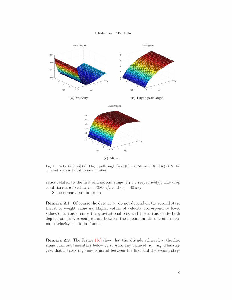
Fig. 1. Velocity [m/s] (a), Flight path angle [deg] (b) and Altitude [Km] (c) at tb1 fordifferent average thrust to weight ratios
ratios related to the first and second stage (n1, n2 respectively). The dropconditions are fixed to V0 = 280m/s and γ0 = 40 deg.
Some remarks are in order:
Remark 2.1. Of course the data at tb1 do not depend on the second stagethrust to weight value n2. Higher values of velocity correspond to lowervalues of altitude, since the gravitational loss and the altitude rate bothdepend on sin γ. A compromise between the maximum altitude and maxi-mum velocity has to be found.
Remark 2.2. The Figure 1(c) show that the altitude achieved at the firststage burn out time stays below 55 Km for any value of nb1 , nb2 . This sug-gest that no coasting time is useful between the first and the second stage
6
DOI: 10.1685/CSC09270
34
56
78
2
3
4
5
65600
5800
6000
6200
6400
nb1
Velocity (m/s) at tb2
nb2
(a) Velocity
34
56
78
2
3
4
5
6−30
−20
−10
0
10
20
nb1
Fpa (deg) at tb2
nb2
(b) Flight path angle
34
56
78
2
3
4
5
6−200
−100
0
100
200
300
nb1
Altitude (Km) at tb2
nb2
(c) Altitude
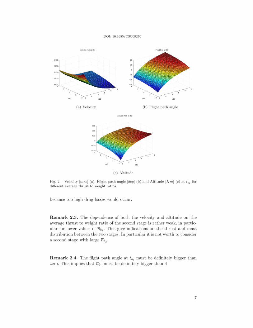
Fig. 2. Velocity [m/s] (a), Flight path angle [deg] (b) and Altitude [Km] (c) at tb2 fordifferent average thrust to weight ratios
because too high drag losses would occur.
Remark 2.3. The dependence of both the velocity and altitude on theaverage thrust to weight ratio of the second stage is rather weak, in partic-ular for lower values of nb1 . This give indications on the thrust and massdistribution between the two stages. In particular it is not worth to considera second stage with large nb2 .
Remark 2.4. The flight path angle at tb1 must be definitely bigger thanzero. This implies that nb1 must be definitely bigger than 4
7
L.Ridolfi and P.Teofilatto
The inspection of these Figures, as well as similar Figures obtained withdifferent dropping conditions V0, γ0, allows to determine suitable values ofn , hence of n0, for each of the stages. These choices determine also thevalues of velocity, flight path angle and altitude, in particular at the burnout times.
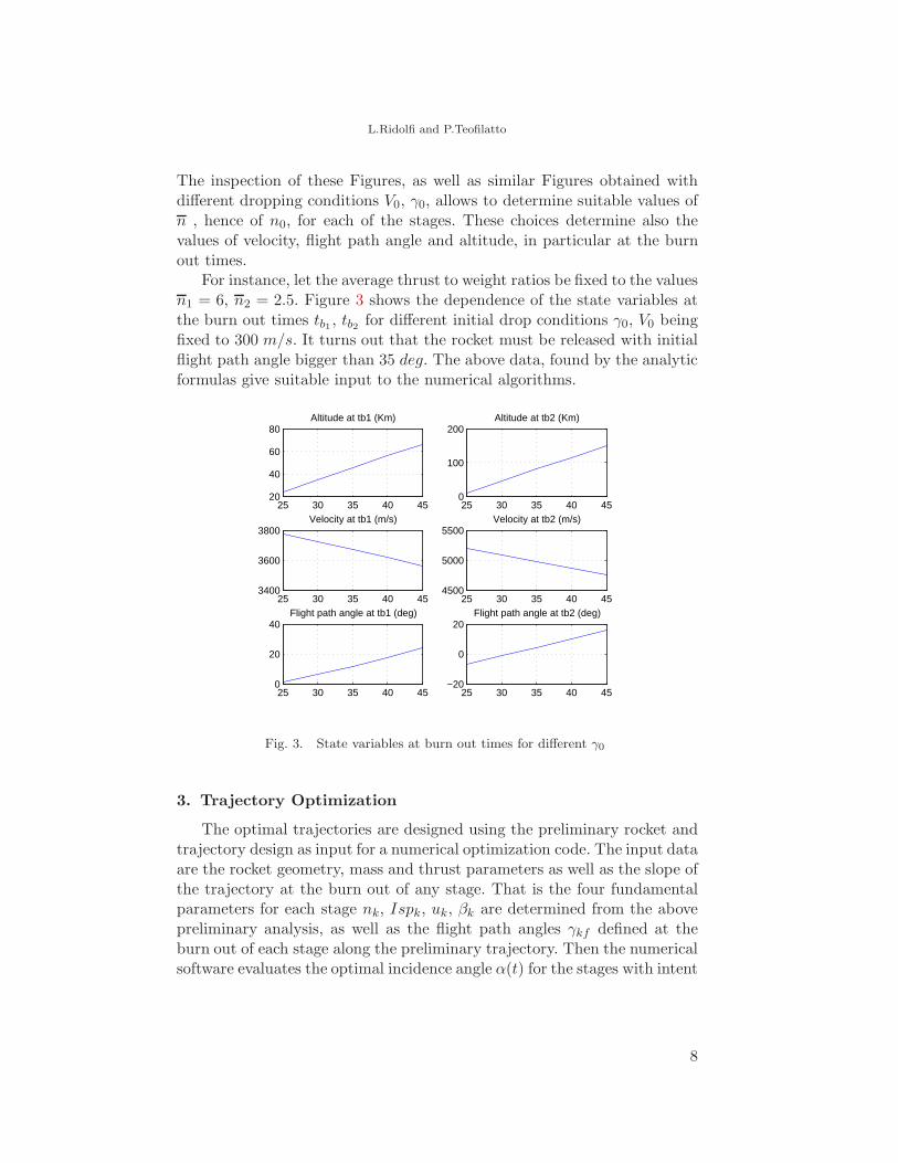
For instance, let the average thrust to weight ratios be fixed to the valuesn1 = 6, n2 = 2.5. Figure 3 shows the dependence of the state variables atthe burn out times tb1 , tb2 for different initial drop conditions γ0, V0 beingfixed to 300 m/s. It turns out that the rocket must be released with initialflight path angle bigger than 35 deg. The above data, found by the analyticformulas give suitable input to the numerical algorithms.
25 30 35 40 4520
40
60
80Altitude at tb1 (Km)
25 30 35 40 450
100
200Altitude at tb2 (Km)
25 30 35 40 453400
3600
3800Velocity at tb1 (m/s)
25 30 35 40 454500
5000
5500Velocity at tb2 (m/s)
25 30 35 40 450
20
40Flight path angle at tb1 (deg)
25 30 35 40 45−20
0
20Flight path angle at tb2 (deg)
Fig. 3. State variables at burn out times for different γ0
3. Trajectory Optimization
The optimal trajectories are designed using the preliminary rocket andtrajectory design as input for a numerical optimization code. The input dataare the rocket geometry, mass and thrust parameters as well as the slope ofthe trajectory at the burn out of any stage. That is the four fundamentalparameters for each stage nk, Ispk, uk, βk are determined from the abovepreliminary analysis, as well as the flight path angles γkf defined at theburn out of each stage along the preliminary trajectory. Then the numericalsoftware evaluates the optimal incidence angle α(t) for the stages with intent
8

DOI: 10.1685/CSC09270
of maximizing the final stage velocity while satisfying the constraints on thefinal slope.
The optimization software employs a standard function for the evalu-ation of constrained minima of functionals in the following fashion: giventhe guess for the incidence law, the software calculates the trajectory andevaluates the cost function and the constraint violations, which are thenused to generate a better guess for the incidence law. Now a Kepleriangravitational field is considered and the aerodynamic effects are taken intoaccount. The aerodynamic coefficients are evaluated using the USAF Mis-sile Datcom Software [10]. In particular the software was used to calculatethe coefficients for a set of flight conditions at different Mach numbers andangles of attack; then the simulation software interpolates the aerodynamiccoefficients. Generally the optimization of the last stage (liquid propellantengine) is performed using the thrust arc intervals as parameters and theoptimization is performed in order to maximize the final mass. The con-straint associated to the final stage is represented by the fulfillment of theterminal conditions related to the insertion into the desired orbit.Practicalengineering constraints are also introduced, e.g. a minimum of one secondof coasting times after the stages burn out in order to allow a safe stageseparation. Moreover, additional coasting times are considered in order toobtain better performances.
Definitely, the optimization of the entire trajectory of a three stagesrocket is made dependent on the selection of the following parameters: thefinal slopes of the first two stages γ1f , γ2f , the coasting intervals betweenthe first and second stage and between the second and the third stage, thethrust arc intervals of the third stage. The algorithm proposed is rathereffective despite its simplicity, and it has been applied to define suitablerocket configurations
4. Performances of EFA Launched Systems
The above analytic and numeric analysis has been applied to the Eu-ropean Fighter Aircraft (EFA), used as carrier aircraft of a rocket able toset same payload into orbit. According to the EFA characteristic and pilotexperience, EFA is able to drop a rocket of 4070 Kg at velocity between280/300 m/s, flight path angle of 40 deg and altitude equal to 12 Km. Ifa three stage rocket is considered, the above analysis gives for the first andsecond stages [3] :
n01 = 3.4 , tb1 = 60 s , n02 = 2.4 , tb2 = 60 s
and the following values of velocity, flight path angle and altitude at theburn out times are achieved:
9
L.Ridolfi and P.Teofilatto
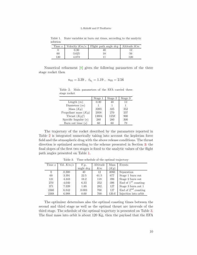
Table 1. State variables at burn out times, according to the analyticsolution
Time s Velocity Km/s Flight path angle deg Altitude Km
0 0.30 40 1260 3.625 18 56120 4.873 11 120
Numerical refinement [8] gives the following parameters of the threestage rocket then
n01 = 3.39 , tb1 = 1.19 , n03 = 2.56
Table 2. Main parameters of the EFA carried threestage rocket
Stage 1 Stage 2 Stage 3
Length (m) 0.30 40 12Diameters (m) 1 1 1
Mass (Kg) 3393 325 352Propellant mass (Kg) 2958 270 237
Thrust (Kgf) 13804 1258 900Specific Impulse (s) 280 280 300Burn out time (s) 60 60 79
The trajectory of the rocket described by the parameters reported inTable 2 is integrated numerically taking into account the keplerian forcefield and the atmospheric drag with the above release conditions. The thrustdirection is optimized according to the scheme presented in Section 3: thefinal slopes of the first two stages is fixed to the analytic values of the flightpath angles presented on Table 1.
Table 3. Time schedule of the optimal trajectory
Time s Vel. Km/s F.p. Altitude Mass Eventsangle deg Km (Kg)
0 0.300 40 12 4060 Separation60 3.391 22.5 61.5 677 Stage 1 burn out121 4.343 18.2 118 396 Stage 2 burn out
270 4.040 6.33 252 396 End of 1st coasting371 7.339 1.89 282 127 Stage 3 burn out 1
2366 6.842 0.003 700 127 End of 2nd coasting2368 6.988 0.00 700 120.6 Injection into orbit
The optimizer determines also the optimal coasting times between thesecond and third stage as well as the optimal thrust arc intervals of thethird stage. The schedule of the optimal trajectory is presented on Table 3.The final mass into orbit is about 120 Kg, then the payload that the EFA
10

DOI: 10.1685/CSC09270
carried rocket can inject into an orbit of 700 Km is between 40 and 50 Kg(depending on the technological level of the liquid propelled engine of thethird stage).
5. Final Remarks
Trajectory optimization is a rather lengthly process based on the pre-liminary knowledge of some parameters that must be refined by iterativenumerical algorithms to achieve the convergence to an optimal solution. Itis important to have some fast tool to get these preliminary results, mainlyin the early phase of a new project when the past experiences are of littleuse and many different options must be investigated. In fact this is the caseof launch systems released from an high performance aircraft.
Analytical formulas have been used to get first guess conditions of op-timal trajectories of air-dropped rocket. These formulas are based on avery simple model: the analytical trajectory is obtained in the hypothesisof gravity turn guidance and no aerodynamic effects. These effects are re-duced at the altitudes where an air-dropped rocket is released and althoughthe gravity turn guidance is not optimal, the analytic formulas are able toprovide a preliminary rocket design and rocket optimal trajectory. Namelythe state variables reported in Tables 1 and 3 show that the analytic formu-las provide with values that are good enough to get numerical convergenceto the actual optimal trajectory.
The method presented here has been applied for different launch sys-tems, based on different carrier aircraft and different dropping conditions.In particular it is shown that EFA launched rocket can inject up to 50 Kminto circular orbits of 700 Km of altitude.
REFERENCES
1. L. Cesari, Optimization - Theory and Applications. Springer Verlag,New York, 1983.
2. A. Ferri, The launch of space vehicles by airbreathing lifting stages, InVistas in Astronautics, Vol. 2 Pergamon Press, London, 1958.
3. P. Teofilatto, P. Cesolari, A ready to launch system by EFA carriedsmall rocket, In First Conference Military Space: Questions in Europe,Paris, 2005.
4. M. Rigault et al., MLA airborne micro-launcher a candidate for alde-baran, IAF Paper IAC-08-D.2.4.9, AIAA Preston, 2008.
5. T. Chen, W. Preston, W. Preston, D. Deamer, J. Hensley , Responsiveair launch using F-15 Global Strike Eagle, In Fourth Responsive SpaceConference, Los Angeles, 2006.
11

L.Ridolfi and P.Teofilatto
6. A. Degtyarev, O. Ventskovsky, Youshnoye perspective luanch systems,IAF Paper IAC-06-D.2.1.04, AIAA Preston, 2006.
7. J. Woo Lee, K. Ho Noh, Y. Hwan Byun , Preliminary design of the hy-brid air launching rocket for nanosat, In Fifth International Conferenceon Computational Science and Applications, Los Angeles, 2007.
8. P. Teofilatto, L. Ridolfi , Effect of different flight conditions at therelease of a small spacecraft from a high performance aircraft, IAF PaperIAC-08-B.4.5.4, AIAA Preston 2008.
9. G. Culler, B. Friend. Universal gravity turn trajectories Journal of Ap-plied Physics , 18 (1957), pp. 672–676.
10. E. Walter , Design methodologies for space transportation systems .AIAA Educational Series, Reston, 2001.
12