Embed Size (px)
Citation preview
AN ANALYSIS OF ISSUES RELATED TO ECONOMIES OF SIZE IN
SASKATCHEWAN CROP FARMS
A Thesis Submitted to the Faculty of
Graduate Studies and Research
In Partial Fulfillment of the Requirements
For the Degree of Masters of Science
In the
Department of Agricultural Economics
University of Saskatchewan
Saskatoon, Saskatchewan
By
Byambatseren Dashnyam
©Copyright Byambatseren Dashnyam, June 2007. All rights reserved

PERMISSION TO USE
In presenting this thesis in partial fulfilment of the requirements for a Postgraduate degree
from the University of Saskatchewan, I agree that the libraries of this University may
make it freely available for inspection. I further agree that permission for copying of this
thesis in any manner, in whole or in part, for scholarly purpose may be granted by the
professor or professors who supervised my thesis work or, in their absence, by the Head
of the Department or the Dean of the College in which my thesis work aw done. It is
understood that any copying or publication or use of this thesis or parts thereof for
financial gain shall not be allowed without my written permission. It is also understood
that due recognition will be given to me and the University of Saskatchewan in any
scholarly use that may be made of any material in this thesis.
Request for permission to copy or make use of material in this thesis in whole or part
should be addressed to:
Head of the Department of Agricultural Economics
University of Saskatchewan
51 Campus drive
Saskatoon, Saskatchewan
S7N 5A8
i
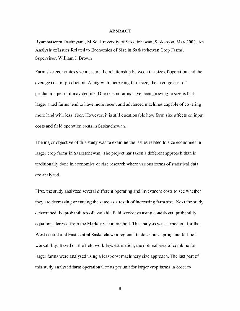
ABSRACT
Byambatseren Dashnyam., M.Sc. University of Saskatchewan, Saskatoon, May 2007. An
Analysis of Issues Related to Economies of Size in Saskatchewan Crop Farms.
Supervisor. William J. Brown
Farm size economies size measure the relationship between the size of operation and the
average cost of production. Along with increasing farm size, the average cost of
production per unit may decline. One reason farms have been growing in size is that
larger sized farms tend to have more recent and advanced machines capable of covering
more land with less labor. However, it is still questionable how farm size affects on input
costs and field operation costs in Saskatchewan.
The major objective of this study was to examine the issues related to size economies in
larger crop farms in Saskatchewan. The project has taken a different approach than is
traditionally done in economies of size research where various forms of statistical data
are analyzed.
First, the study analyzed several different operating and investment costs to see whether
they are decreasing or staying the same as a result of increasing farm size. Next the study
determined the probabilities of available field workdays using conditional probability
equations derived from the Markov Chain method. The analysis was carried out for the
West central and East central Saskatchewan regions’ to determine spring and fall field
workability. Based on the field workdays estimation, the optimal area of combine for
larger farms were analysed using a least-cost machinery size approach. The last part of
this study analysed farm operational costs per unit for larger crop farms in order to
ii

determine how machinery efficiency and farm size have an effect on the farm production
costs.
The study found that however there were certain combine costs that increase with farm
size in Saskatchewan. In addition, soil types, weather conditions and field efficiency can
strongly affect combine cost per acre.
The results of this research provide a reference for policy makers in designing policy
recommendations. In addition, the results may offer useful information for farmers in
designing management plans to control farm operation costs.
iii

ACKNOWLEDGEMENTS
I wish to thank and acknowledge my supervisor, Prof. William, J. Brown. Without his
expertise, guidance, and advice, the goals of this thesis would have been much more
difficult to obtain. His efforts in providing me with constant feedback and encouragement
are greatly appreciated. I also wish to thank my committee members Prof. Richard Gray
and Jackson Clayton for their patience and help with various aspects of the farm
analysis.
Special thanks are extended to the Department of Agricultural Economics for providing
financial support throughout the study and Chokie Mengisteab for his valuable advice
and help with the statistical analysis.
My sincere gratitude is extended to my wife, Tuyana, my daughters Egshiglen and
Elizabeth for their love and encouragement to do my best during my entire life. This thesis
is dedicated to them.
iv
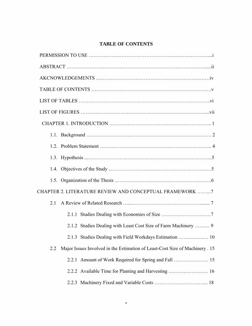
TABLE OF CONTENTS
PERMISSION TO USE ………………………………………………………………....i
ABSTRACT ………………………………………………………………………….....ii
AKCNOWLEDGEMENTS ……………………………………………………………iv
TABLE OF CONTENTS ……………………………………………………………….v
LIST OF TABLES ……………………………………………………………………..vi
LIST OF FIGURES …………………………………………………………………....vii
CHAPTER 1. INTRODUCTION …………………………………………………….. 1
1.1. Background …………………………………………………………………. 2
1.2. Problem Statement ………………………………………………………….. 4
1.3. Hypothesis ...………………………………………………………….……...5
1.4. Objectives of the Study ...……………………………………………………5
1.5. Organization of the Thesis …………………………………………….…….6
CHAPTER 2. LITERATURE REVIEW AND CONCEPTUAL FRAMEWORK ……...7
2.1 A Review of Related Research …...……………………………………....... 7
2.1.1 Studies Dealing with Economies of Size …………………………7
2.1.2 Studies Dealing with Least Cost Size of Farm Machinery ……… 9
2.1.3 Studies Dealing with Field Workdays Estimation ……………… 10
2.2 Major Issues Involved in the Estimation of Least-Cost Size of Machinery . 15
2.2.1 Amount of Work Required for Spring and Fall ………………… 15
2.2.2 Available Time for Planting and Harvesting …………………… 16
2.2.3 Machinery Fixed and Variable Costs …………………………... 18
v
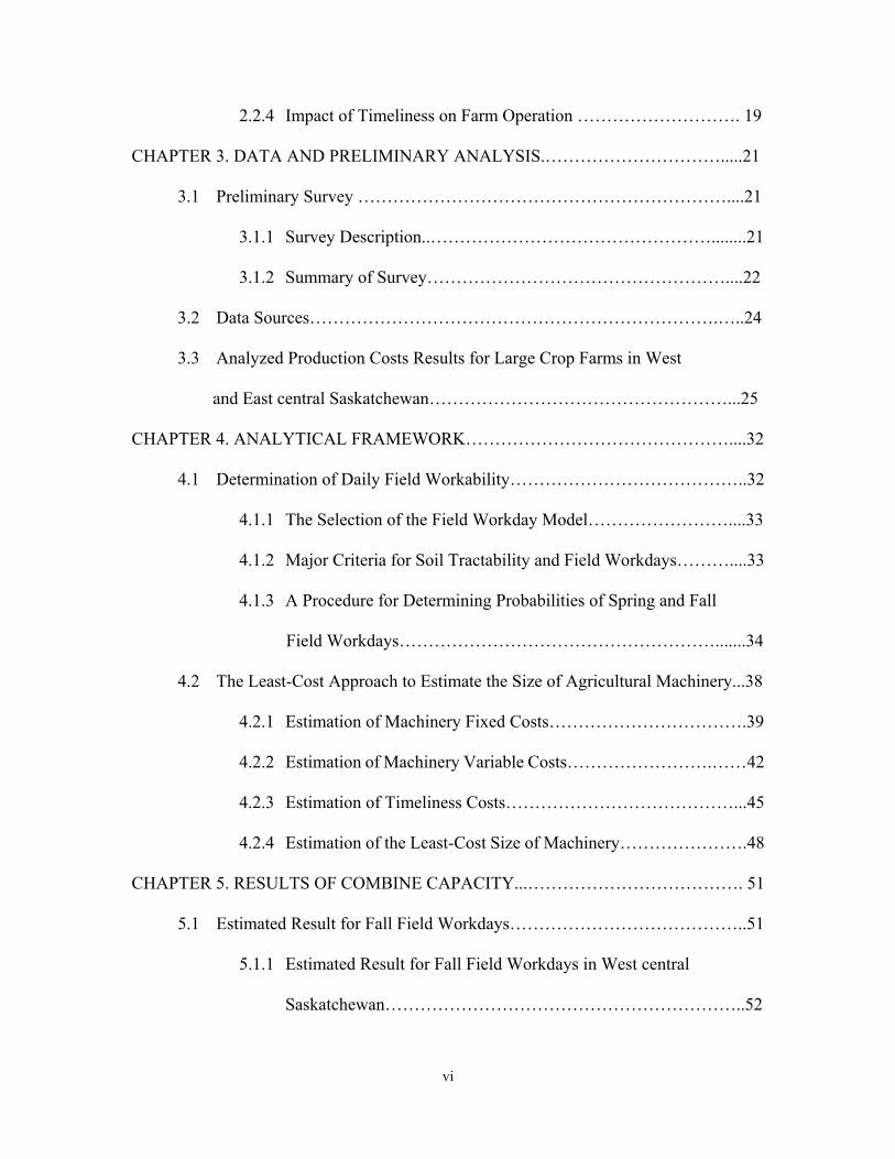
2.2.4 Impact of Timeliness on Farm Operation ………………………. 19
CHAPTER 3. DATA AND PRELIMINARY ANALYSIS.………………………….....21
3.1 Preliminary Survey ………………………………………………………....21
3.1.1 Survey Description..…………………………………………........21
3.1.2 Summary of Survey……………………………………………....22
3.2 Data Sources…………………………………………………………….…..24
3.3 Analyzed Production Costs Results for Large Crop Farms in West
and East central Saskatchewan……………………………………………...25
CHAPTER 4. ANALYTICAL FRAMEWORK………………………………………....32
4.1 Determination of Daily Field Workability…………………………………..32
4.1.1 The Selection of the Field Workday Model……………………....33
4.1.2 Major Criteria for Soil Tractability and Field Workdays………....33
4.1.3 A Procedure for Determining Probabilities of Spring and Fall
Field Workdays……………………………………………….......34
4.2 The Least-Cost Approach to Estimate the Size of Agricultural Machinery...38
4.2.1 Estimation of Machinery Fixed Costs…………………………….39
4.2.2 Estimation of Machinery Variable Costs…………………….……42
4.2.3 Estimation of Timeliness Costs…………………………………...45
4.2.4 Estimation of the Least-Cost Size of Machinery………………….48
CHAPTER 5. RESULTS OF COMBINE CAPACITY...………………………………. 51
5.1 Estimated Result for Fall Field Workdays…………………………………..51
5.1.1 Estimated Result for Fall Field Workdays in West central
Saskatchewan……………………………………………………..52
vi
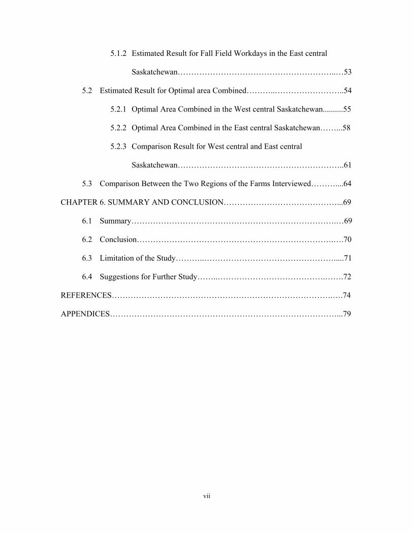
5.1.2 Estimated Result for Fall Field Workdays in the East central
Saskatchewan…………………………………………………..…53
5.2 Estimated Result for Optimal area Combined………..……………………..54
5.2.1 Optimal Area Combined in the West central Saskatchewan..........55
5.2.2 Optimal Area Combined in the East central Saskatchewan……...58
5.2.3 Comparison Result for West central and East central
Saskatchewan……………………………………………………..61
5.3 Comparison Between the Two Regions of the Farms Interviewed………....64
CHAPTER 6. SUMMARY AND CONCLUSION……………………………………...69
6.1 Summary………………………………………………………………….…69
6.2 Conclusion……………………………………………………………….….70
6.3 Limitation of the Study………..………………………………………….....71
6.4 Suggestions for Further Study……..………………………………….…….72
REFERENCES……………………………………………………………………….….74
APPENDICES…………………………………………………………………………...79
vii
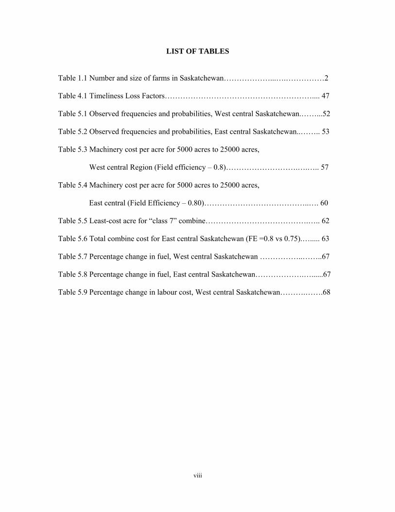
LIST OF TABLES
Table 1.1 Number and size of farms in Saskatchewan………………...….……………2
Table 4.1 Timeliness Loss Factors………………………………………………….... 47
Table 5.1 Observed frequencies and probabilities, West central Saskatchewan.……...52
Table 5.2 Observed frequencies and probabilities, East central Saskatchewan..…….. 53
Table 5.3 Machinery cost per acre for 5000 acres to 25000 acres,
West central Region (Field efficiency – 0.8)……………………….….….. 57
Table 5.4 Machinery cost per acre for 5000 acres to 25000 acres,
East central (Field Efficiency – 0.80)…………………………………..…. 60
Table 5.5 Least-cost acre for “class 7” combine………………………………….….. 62
Table 5.6 Total combine cost for East central Saskatchewan (FE =0.8 vs 0.75).…..... 63
Table 5.7 Percentage change in fuel, West central Saskatchewan ……………..……..67
Table 5.8 Percentage change in fuel, East central Saskatchewan……………….…......67
Table 5.9 Percentage change in labour cost, West central Saskatchewan……….…….68
viii

LIST OF FIGURES
Figure 1.1 Distribution of Grain and Oilseed Farms……………………………..………2
Figure 1.2 Concentration of Production, Grain and Oilseed Farms, 1998………..……...3
Figure 3.1 Sales Income per Acre…………………………………………………….…26
Figure 3.2 Net Income per Acre…………………………………………………………27
Figure 3.3 Total Expense per Acre………...…………………………………….…….. 27
Figure 3.4 Total Wage per Acre………………………………………………………...28
Figure 3.5 Fertilizer Expense per Acre………………………………………………….29
Figure 3.6 Herbicide Expense per Acre………………………………………………....29
Figure 3.7 Fuel Expense per Acre………………………………………………….…....30
Figure 3.8 Repair and Maintenance Expense per Acre…………………………….…....31
Figure 3.9 Machinery Assets per Acre…………………………………………….….....31
Figure 4.1 Yield of Wheat, Durum and Flax at Saskatoon……………………………...47
Figure 5.1 Machinery cost per acre, West central Region Saskatchewan………….........56
Figure 5.2 Minimum total combine cost for class 5, 7 and 8……………………………56
Figure 5.3 Machinery cost per acre, East central Saskatchewan…….………………….61
Figure 5.4 Total Rotational Expense per Acre, West central Saskatchewan………........65
Figure 5.5 Total Rotational Expense per Acre, East central Saskatchewan…….……....66
ix

CHAPTER 1
INTRODUCTION
1.1 Background
Crop production in Saskatchewan is vulnerable to unpredictable climatic conditions
and variability in global market conditions. For these reasons, the farming sector in
Saskatchewan faces numerous challenges. For instance, a lack of moisture combined
with hot, dry and windy summers often lead to poor growing conditions and low
yields. As well, a booming oil industry in the neighboring province of Alberta has
caused a labour shortage, which adversely affects farm businesses in Saskatchewan.
The face of Saskatchewan agriculture continues to change. Since the 1940s, the
number of farms in Saskatchewan and Canada has been declining (Statistic Canada,
2001). Although agriculture's share of the economy has declined steadily for the last
few decades, Saskatchewan continues to represent an important element of Canadian
agriculture. For example, in 2004, 20.5 percent of Canada’s 246,923 farms were
located in Saskatchewan. According to statistics from the 2001 Canadian Census of
Agriculture, while the number of farms operating in Canada continues to decline,
they are producing more output (Census Stat Fact, 2001).
Grain and oilseed farms represent an important component of Saskatchewan
agriculture. This can be seen from the number of farms in the province which produce
grains and oilseeds (Census Stat Facts, 2001). Even as the number of the farms has
been declining rapidly, Saskatchewan still has the highest concentration of grain and
1

oilseed farms of any province (Table 1.1). In 1998, about half of the grain and oilseed
farms with revenue of $10,000 or more were located in Saskatchewan, accounting for
approximately 47% of total grain and oilseed farms nationally (Figure 1.1).
Table 1.1 Number and size of farms in Saskatchewan
Year 1931 1941 1951 1961 1971 1981 1991 2001
Grain and oilseed farms 136,472 138,713 112,018 93,924 76,970 67,318 60,840 32,774
Average farm land (acres) 408 432 550 686 845 974 1,091 1,283
Source: Statistics Canada Census of Agriculture 2001.
Manitoba12%
Alberta22%
OtherProvince
4%Ontario
15%
Saskatchewan47%
Source: Statistics Canada, Whole Farm Data Base, 2002
Figure 1.1 Distribution of Grain and Oilseed Farms With Revenue of $10,000 or
More
2

The size of farms in Saskatchewan increased during the second half of the 20th
century (Table 1.1). For instance, in Saskatchewan, the average farm size has grown
from 1,091 acres in 1991 to 1,283 acres in 2001, increasing by almost 212 acres in 5
years (Table 1.1). In addition, the share of large sized farms with revenues of
$100,000 to $249,999 has remained relatively steady throughout the 1990s,
accounting for around one third of total production by grain and oilseed farms
(Agriculture and Agri-Food Canada, 2001). The share of production by very large
farms with revenues of $500,000 or more is 16.0% and only 2.2% of grain farms in
Canada belong to the very large farm category in 1998 (Figure 1.2). Grain and
Oilseed production is becoming heavily concentrated on farms with revenue of
$100,000 or more.
42.9
22.9 24.5
7.72.2
10.015.0
35.5
23.5
16.0
0
10
20
30
40
50
$10,000 to$49,999
$50,000 to$99,999
$100,000 to$249,999
$250,000 to$499,999
$500,000 andover
%
Percent of farm Percent of Total Production
Source: Statistics Canada, Whole Farm Data Base, 2002
Figure 1.2 Concentrations of Production, Grain and Oilseed Farms, Canada 1998
3

1.2 Problem Statement
Grain and oilseed farm size has changed rapidly in recent years in Saskatchewan.
With changing farm size, large grain and oilseed farms are acquiring larger more
complex machines in their operations. Related to the size trend, there are
comparatively few recent studies that address issues related to economies of size
(EOS) and machine costs in farm production. Although some studies have been
completed, they have usually studied all sizes of farm operations. In reality, farm
production cost economies of large grain and oilseed farms has been a relatively
unstudied topic in Saskatchewan.
Farm size is an important factor for production efficiency when it comes to
commodity based agriculture. Theoretically, high profit crop farms are consistently
bigger than low profit crop farms due to the bigger sized farms taking advantage of
economies of size and spreading fixed costs over a larger farm area. Very large farms
may also get discounts on the purchase price of machinery investments. As well
these very large farms may also be able to capture discounts on variable costs like
fuel, fertilizer, chemicals and transportation costs. Even within the group of very
large farms, there are considerable differences in financial outcomes. The data from
Statistic Canada demonstrates a significant difference in expenditures per dollar of
sales for very large sized crop farms between the top 20% and bottom 20% (Statistics
Canada, 2005).
4

As related above, the size of crop farms have been growing rapidly in Saskatchewan,
not all of these larger farms have been successful and sometimes large farms get into
financial problems or decide to exit agriculture. This increasing size trend raises an
important question: does farm size matter for economic efficiency? In order to study
economic efficiency connected with farm size, components of farm costs must be
taken into account.
Issues related to size of economies deal with the relationship between production
costs and size. There are several interrelated questions which relate to farm size and
costs. These questions include: what operating and investment costs per acre are
decreasing, increasing and staying the same as a result of growing farm size? Do
large crop farms use machinery more efficiently? How does available field workday
affect least-cost machinery size? This study will address these issues for
Saskatchewan crop farms. Answering these questions would provide farm policy
makers with useful information for the future development of farm policy.
1.3 Hypothesis
The hypothesis of this study is that larger crop farms differ from smaller farms with
respect to economies of size.
1.4 Objective of the Study
The primary objective of this study is to analyse issues related to size economies in
larger crop farms in Saskatchewan. More specifically, the objectives of this study are:
5

1. Examine several different farm operating and investment costs and state whether
they are decreasing or staying the same as a result of increasing the farm size.
2. Estimate the probabilities of spring and fall field workdays for crop farms in the
east central and west central areas of Saskatchewan.
3. Identify and compare optimal combine capacity for large crop farms in the west
central and east central areas.
4. Calculate the effect of harvest machinery size and investment on large crop farm
production costs.
1.5 Organization of the Thesis
The study has six chapters. A review of the literature related to economies of size as
well as the major issues involved in the estimation of least-cost size of machinery is
presented in chapter two. Chapter 3 presents farm financial survey and data sources
used. Also, the summary of managers of large crop farms interviewed is described in
this chapter. Techniques for determining probabilities of field workdays, optimal size
of machinery and the farm operation and investment costs is discussed in chapter 4.
Chapter five presents the results for field workdays in the west central and the east
central areas as well as results for machinery efficiency and comparison of large
farms. The final chapter contains the summary and conclusion of the study. Possible
further research areas and limitation of the study are provided in the final chapter.
6
CHAPTER 2
LITERATURE REVIEW AND CONCEPTUAL FRAMEWORK
2.1 A Review of Related Research
This literature review focuses on three subjects related to the research questions. The
first section reviews studies dealing with farm economies of size. Studies presenting
analytical models for estimating the optimal size of farm machinery are reviewed
next. Finally, studies providing methodological guidance on how to measure
available field workdays at the farm level and provide methodological guidance are
reviewed.
2.1.1 Studies Dealing with Farm Size and Economies of Size
Numerous studies employing a variety of techniques and methods have been
undertaken to obtain information on size and scale economies for various industries.
In general, several methods are commonly cited: descriptive analysis, economic
engineering, average function analysis and frontier function analysis (Ker and
Howard, 1993). For the agricultural sector, there are several studies on farm
economies of size carried out in the 1990s mostly using an average functional
approach or frontier function approach to model economies of size and scale.
Although most of the early studies deal with general farming, with regard to the
relationship between economic efficiency and crop farm sizes, a review of these
studies is still important in order to provide a framework for establishing appropriate
methodology and concepts.
7
Kumbhakar (1993) studied the effects of returns to scale, farm-size and economic
efficiency of Utah dairy farms using a generalized production function and concluded
that large farms are relatively more efficient than small and medium-sized farms. He
argued that the growth of large farms may be explained in terms of economic
efficiency. In addition, small farms are less efficient than medium and large-sized
farms and large farms can deal with a decrease in output price or an increase in input
price better than smaller-sized farms. This is consistent with early research work that
demonstrated that optimum size differs between farms depending on the stock of
labour, capital and management possessed in each farm (Heady, 1958), and existing
family farms economies of size soon give away to diseconomies (Hall and Leveen,
1978).
Aly et al. (1987) estimated a deterministic statistical production frontier function for a
sample of Illinois crop farms. They found that larger farms tend to be more
technically efficient than smaller farms, Conversely Byrnes et al. (1987) examined
grain farm efficiency in the same region and revealed larger farms in the sample to be
slightly less technically efficient than smaller grain farms. Finally, Garcia et al.
(1982) studied the relationship between technical efficiency in the same region and
farm size. They found that smaller farms in their sample were as economically
efficient as large farms. The major conclusion that can be carried out from reviewing
these studies is the lack of clear evidence on both the level of average technical
efficiency of crop farms and the relationship between technical efficiency and farm
8

size. This mixed empirical result can be the result of temporal events such as weather,
which could significantly change the estimated efficiency from one year to another.
Kalaitzandonakes et al., (1992) analyzed the efficiency levels of a sample of Missouri
grain farms by applying alternative frontier estimation procedures. In this study, the
three different estimation approaches are found to significantly alter the levels of
technical efficiency for each individual farm in the sample. They suggested that
“mixed empirical evidence on the relationship between farm size and technical
efficiency of grain farms found in recent literature is the result of variation in the
estimation procedures employed” (p. 439). As well, their evidence supports that there
is a positive relationship between farm size and technical efficiency, and an average
larger farm can harvest more yield than smaller farms from a given amount of input.
2.1.2 Studies Dealing with Least-Cost Size of Farm Machinery
Various studies have linked determining optimal size of machinery and how this
optimal size of machinery is an essential contributor to farm efficiency. Some of this
research has been recognized as vitally important to the current study. There are two
significant studies on least-cost size of farm machinery referred to here, namely
Brown and Schoney (1985) and Henning and Claus (2004).
Brown and Schoney studied proper machinery sizing for a given farm and found the
least-cost combination of machinery taking into account fixed, variable and
timeliness costs. In the study, they reviewed three different machinery size models
and recommended the least-cost model can be a relatively simple model that
9
calculates the least-cost combination of machines for a given farm situation. They
selected an 1800 acre grain farm in Saskatchewan and minimized the sum of fixed,
variable and timeliness costs for the entire farm machinery complement.
Henning and Claus (2004) developed a system model to support the process of
choosing the optimal level of farm mechanisation in terms of technical capability.
“The optimisation model is a non-linear programming model implemented by using
the programming software suite General Algebraic Modelling System”(p. 13). The
model is based upon a least-cost concept involving all expected fixed and variable
costs (including timeliness costs) for a particular farm size and crop plan. The output
from the model is the sizing of each machine, and also the tractor power and number
of tractors required. They have shown the effective work rates of the machinery sets
and the duration in nominal time for performing each operation. The selection is
based upon a farm-oriented matrix involving various types of constraints, such as
available man-hours, available machine- and tractor-hours, timeliness and workability
of operations, agronomic window of operations, and sequence of operations. The
model was tested and verified for its operational behaviour using real farm data. They
stated that although there are a variety of factors that can affect minimum machinery
costs, operators always optimize farm machinery connected to these aspects. In real
life, some of the actual machines are not optimally sized.
2.1.3 Studies Dealing with Field Workdays Estimation
Field workdays are based on soil and weather conditions that indicate suitability of
completing field work on a given day. The concept of a field workday has been an
10
important part of field work and machinery needs on an individual farm basis. There
have been a number of significant studies on the field workability and tractability
carried out in the last few decades. These studies mostly discuss the importance of
soil workability for crop production, and review the limitations of a variety of
models, especially their applicability for predicting the effects of climate change.
These field workability models can be classified into two different groups. Most
researchers employ models that can calculate the number of spring or autumn
workdays by combining meteorological and soil related factors. During the late 1960s
and early 1970s several work-day models were formulated, which differ in their
interpretation of workability from climatic variables and rely on various model
inputs. Rounsevell (1993) concludes these were similar studies because precipitation
was the overall controlling influence. The work of Amir et al. (1976) and Smith
(1970, 1977) demonstrate the simplest of this category of models.
Amir et al. studied the probabilities of available field workdays using 40 years of
recorded climatological data. First, they determined various types of calculated
probabilities using observed data. Then results were tested by paired t-statistic tests to
determine whether or not the observed and the calculated probabilities have the same
mean. The result found that at the α = 0.05 level of significance that the two sets have
the same mean for every month. The procedure described in this paper uses
conditional probability equations derived from the Markov Chain method. However,
this procedure is only as precise as the model from which it derives. Soil type and the
model’s suitability were completely ignored in this approach because only
11

precipitation data was used to determine field workdays. Therefore, the value of this
model for estimating workability for a range of climates and soils is in doubt.
In Smith’s (1977) model, land was divided into light medium and heavy soil textural
classes, and for each class a set of empirical criteria were employed which
determined the suitability of a spring day for working. The criteria considered only
the amount of precipitation and occurrence of rainfall though different limits were
imposed for each soil group. Although large errors were found in the prediction of
field workdays, he attributed this result to soil variability within the simplified soil
groupings and accepted that land at the boundary of a textural class would inevitably
be subject to error.
Ruthledge and McHardy (1968) used a simplified version of the Versatile Soil
Moisture Budget (VSMB) for estimating work and non-workday probabilities for
seven stations in Alberta with light to heavy soils. They assumed a four inch soil
moisture storage capacity distributed over the six zones of the VSMB. They
recommended as criteria for non-workdays estimated soil moisture content in excess
of 95% of field capacity in any of the three upper zones. However, the inclusion of
three zones was justified only in medium or heavy soils. In sandy soils, only two
zones warranted consideration.
Rounsevell (1993) presented a detailed review of previous work on soil workability
and estimation of numbers of workdays for cultivation/tillage-type operations. The
simplest models are based on precipitation alone, but most include some
12

consideration of soil, either as simple soil categories or as a complex consideration of
soil strength. He revealed that some studies looked only at long-term average
workability for broad soil categories or land types. Also, Rounsevell concluded that
there is a reasonable consensus in favour of estimating workdays from some sort of
soil water balance model, with the limiting water content for workability at or near
field capacity.
Rounsevell and Jones (1993) discuss the distinction between workability and
tractability. They define tractability as the capacity of soil to support and withstand
traffic with negligible soil structural damage and no adverse effects on crop yield.
They define workability as the condition in which soil tillage operations such as
ploughing and seedbed preparation can be performed. In the case of seed-bed
preparation conditions need to be suitable for the production of a friable land without
smearing or compaction. They note that workability does not define a precise soil
condition because this depends on the operation, operator, type and size of machine.
Also soil type has a strong influence on the production of a friable tilth in seed-bed
preparation.
McGechan and Cooper (1997) have presented an exploratory study of the role of a
soil-water simulation model for the study of workdays for winter field operations in
the current climate, particularly for the operation of field spreading of animal waste
(slurry) in connection with waste management plans. In this case, as well as soil
water content constraints, the incidences of snow and frozen soil were considered to
avoid runoff pollutants to watercourses, either at the time or later when the thaw
13
occurred. This approach to modeling transport processes of water through the soil is
more mechanistic than the simple soil-independent water balance with empirical
adjustments for soils adopted by Rounsevell and Jones (1993).
Toro and Hansson (2004) studied an assessment of field machinery performance in
variable weather conditions using discrete event simulation. A simulation model for
field machinery operations was developed using a discrete event simulation technique
in order to determine annual timeliness costs in a long-term assessment on cereal
farms, with the results compared with a simpler approach. The experiment on spring
seedbed preparation on a clay soil showed that “the date had only a minor effect on
soil compaction but the fraction of fine aggregates increased with time” (p. 41). The
fine aggregate is defined as containing a high proportion of particles passing a 5mm
sieve. Thus, the optimal time for seedbed preparation depended more on soil friability
than on the risks of compaction.
Although there have been numerous efforts to develop a methodology to determine
available field workdays, there is still not a generally accepted method. The
simulation model for field machinery operations developed using a discrete event
simulation technique enabled timeliness costs and their annual variability to be
estimated in a long-term assessment. In addition, the Toro and Hansson’s study
revealed that the model is particularly appropriate for estimating timeliness costs for
the harvesting operation in conditions of scattered field maturation times and
probable overlapping of their ‘single harvesting periods’, where simpler approaches
are difficult to apply.
14
From the Toro and Hansson’s research, machinery sets with high daily effective field
capacity not only resulted lower timeliness costs but also lower annual variation.
Timeliness costs were more affected by a stepwise reduction in daily effective field
capacity than a stepwise increase of the same magnitude. For given farming
conditions and within certain limits of machinery capacity, there was not just one set
identified as the ‘least-cost’ option. Instead, several sets performed at a similar low
cost level. Higher specific machinery costs for the larger sets were offset by lower
timeliness and labour costs, and the converse was equally true. The machinery set to
be selected should be the largest set among those with a similar ‘least-cost’ on
account of its lower annual variation, which usually implies lower risks.
2.2 Major Issues Involved in the Estimation of the Least-Cost Size of
Machinery
2.2.1 Amount of Work Required for Spring and Fall
An important aspect of purchasing a new machine or tractor is making the decision
on what size of a machine is needed. In order to optimise machinery selection, one
needs to determine the amount of work required in spring and fall. This is one of the
important parts of farm machinery planning. If the amount of work required for
spring seeding and fall harvest could be determined with a reasonable degree of
certainty, machinery selection would be much easier.
The amount of work required for the operation period can be approximated by using
several key factors such as crop acres and yields. Crop acres to be planted are the
main determining elements for amount of work required for spring. However,
15

combinations of crop yield and acres determine how much work has to be done for
fall field work.
The number of acres that can be completed each day is a more dependent on the
measure of machinery capacity than machine width or acres completed per hour. In
some cases, increasing the labour supply by hiring extra operators or by working
longer hours during critical periods may be a relatively inexpensive way of extending
machinery capacity. When the amount of work required for harvest can be anticipated
to require more machinery and labour than the farm’s capacity, farm operators have
to decide whether or not to extend machine power capacity and to hire more labor or
to hire custom work. The cost of additional labour or custom work only needs to be
incurred in those years in which it is actually used, while the cost of investing in
larger machinery becomes “locked in” (Edward and Hanna, 2001(a), pp. 2) as soon as
the investment is made. On the other hand, extra labour and custom work may not
always be available when needed, and working long hours over several days may
reduce labour productivity.
2.2.2 Available Time of Field Operations
Weather patterns partially determine the number of days suitable for field work in a
given time period each year. Although actual weather conditions cannot be predicted
far enough in advance to be used as an aid to machinery selection, past weather
records can be used as a guide. Field workdays are usually expressed on a probability
basis because of the randomness of weather. A 90% probability of a field workday
can be interpreted as meaning that suitable field workdays could be expected in 9 out
16

of 10 days. Thus, machinery selection should be based on long-run weather patterns
even though it results in excess machinery capacity in some years and insufficient
capacity in others.
In addition, total time required for a field operation depends on the capacity of the
machine and the number of available field workdays. Duration of field workdays can
be different depending on the region’s soil type and climate condition. For instance,
wet soil and wet crop conditions require a special kind of field operation which may
result in a delay of harvesting or an increase in operation cost.
The weather data of past years is obviously relevant, on the assumption that past
weather statistics represent a population from which future years will show no
significant deviation (Smith, 1970, p.18). But in some years weather can be
unpredictable. For example, a rainy and cold summer could cause a delayed harvest.
There are some options to deal with a shorten duration of field operations. Working
over time can be one of these options if several operators are available. In addition,
night-time operations have always been done when weather, soil and crop condition
are favorable (Bowers, 1987, p. 121). Modern farm machinery equipped with GPS
helps to facilitate the farm operator’s duties. For instance wide tillage and seeding
machines can be accurately steered without the sighting problems associated with
darkness (Hunt, 2001, p. 276).
Profitable farming operations require strict control of production costs. One approach
to production cost control is purchasing replacement machinery just large enough to
17
complete the required work in the time available. Owning extra machinery capacity is
an added expense, but planting and harvesting delays can also be costly. Presently,
farmers who can produce their product with lower cost survive in the competitive
market. Cost conscious farmers will choose the size of their farm machinery based on
the number of acres to be covered and the number of suitable days to do the required
work. Unfortunately there are large fluctuations in the number of suitable field
workdays from year to year. Thus, farmers must be aware to determine field
workdays and use an appropriate method for a certain region to evaluate available
field workdays.
2.2.3 Machinery Fixed and Variable Costs
Owning and operating machinery remains one of the largest costs in crop production.
Since the price received for agricultural produce has been stable or declining for a
number of years at least in real terms, producers continue to pursue lower cost and
more efficient production systems (Kay et al., 2004, p.398). The development or
selection of optimal machinery systems can help reduce costs while providing timely
field operations that optimize the yield and quality of crops produced. Machinery is
costly to own and operate. Today, a single farm machine may cost several hundred
thousand dollars. Farmers must be cautious of making decisions connected with
owning machinery.
Machinery costs include costs of ownership and operation as well as penalties for
lack of timeliness. Ownership costs tend to be independent of the amount a machine
is used and are often called fixed or overhead costs. Per hectare ownership costs vary
18

inversely with the amount of annual use of a machine. Therefore, a certain minimum
amount of work must be available to justify purchase of a machine and, the more
work available, the larger the ownership costs that can be economically justified.
Conversely, operating costs or variable cost increase by the amount the machine is
used. Total machine costs are the sum of the fixed and variable costs. Total machine
costs can be calculated on an annual, hourly, or per acre basis (Hunt, 1987, p.63).
Total per acre cost is calculated by dividing the total annual cost by the area covered
by the machine during the year.
A custom cost is the price paid for hiring an operator and equipment to perform a
given task. A farm operator can compare total per acre costs to custom costs to
determine whether it would be better to purchase a machine or to hire the equipment
and an operator to accomplish a given task.
2.2.4 Impact of Timeliness on the Farm Operation
There is an optimum time of the year to perform some field operations and economic
penalties are incurred if the operations are performed too early or too late. When
harvesting a crop, for example, increasing fractions of the yield may be lost and/or
the crop quality may be reduced if the harvest is started too early or delayed beyond
the optimum time.
Timeliness costs include lower yields due to delayed planting and harvest date. In
addition, fluctuations in the number and sequence of suitable field workdays from
year to year cause timeliness costs to vary even when the machinery set, number of
19

crop acres and labour supply do not change (Hunt, 2001, p. 274). Investing in larger
machinery can reduce the variability of timeliness costs by ensuring that crops are
planted and harvested on time even in years in which there are few good working
days. However, machinery fixed costs would be higher with larger machinery. Some
farmers may be willing to pay more (in higher fixed machinery costs) than other
operators for the insurance of not suffering substantial yield losses due to late
planting and harvesting in certain years.
20
CHAPTER 3
FARM FINANCIAL SURVEY AND DATA SOURCES
This chapter presents results of the preliminary survey and analysis of production
costs for crop farms in Saskatchewan. The first section presents a description of the
preliminary survey including major results. This is followed by the graphical analysis
of production costs for crop farms in Saskatchewan.
3.1 Preliminary Survey
3.1.1 Survey Description
Saskatchewan crop farms have been getting larger for several decades. There have
always been outliers of a few extremely large farms. Given current profit margins,
crop farms are becoming significantly larger. The traditional notion of the benefits of
increased size is the reduction of machinery fixed costs. Very large farms may also
get volume discounts on the purchase price of machinery. In addition these very large
farms may also be able to capture discounts on variable costs like fuel, fertilizer,
chemicals and trucking fees. Not all of these very large farms have been successful
and the media have made it a major event when one or two get into financial
problems or decide to exit agriculture (Maynard, April 13, 2006).
As part of this research, 13 large crop farms were visited in the west and east central
regions of Saskatchewan. The purpose was to discuss economies of size issues with
the owners of these businesses and to discover the major challenges facing very large
crop farms in Saskatchewan. The producers interviewed were selected by soliciting
their names from various sources known with the Department of Agricultural
21
Economics at the University of Saskatchewan and therefore the sample was not
random. The questions asked dealt with machinery, building investments and
purchases of fuel, fertilizer, and chemicals.
3.1.2 Summary of Survey Results
The discussion indicated that most farmers interviewed felt that their yield per acre
was higher than smaller farms in the area. Factors mentioned that influenced these
higher yields were soil type and input use. Except for one, all farms interviewed had
soil types of clay or clay loam.
Another important factor was the availability of the good quality land to rent. On
average 70% of the land farmed by the interviewees was rented and all on cash rent
basis. The farmers interviewed frequently receive land renting and selling requests
from small and medium sized farms which help them to make better land selection
and to settle the rental rate efficiently. Renting better quality land gives them a better
chance for higher yields. Moreover, the amount and types of inputs per production
unit for those interviewed appears to be significantly higher than typical farms as
shown in SAF’s crop planning guide (SAF, 2006).
Those interviewed generally felt that their yields were higher than others because of
more efficient use of equipment and inputs. In addition, those interviewed felt they
get more discounts on input purchases and more services from input dealers. The
participants farmed between 12,000 and 23,000 acres, and an average combine’s
capacity was between 4,000 and 5,000 acres annually. Most of those interviewed
22

stated that they decide how many acres to rent on the capacity of their machinery.
That is to say, first the farmers make a decision related to machinery sizing, and then
they rent the necessary land. This planning strategy assists those interviewed to use
their machinery more efficiently.
The farmers in the survey generally agreed that they receive some discounts on
certain input purchases because of their size of operation. These discounts ranged
from 5 to 20% for fuel and 1to 5% for fertilizer and chemicals. Those interviewed
also said they save on delivery costs and time and labour costs related to the
purchasing activity. In addition, there are some consulting services that come with
large chemical purchases that help to determine the optimal use of chemicals.
All but one of those interviewed used the same brand of farm machinery. Only three
leased most of their machinery, the rest purchased it. Most traded in by three years,
thereby most of the machines on the farms were under warranty. All those
interviewed stated that timeliness of operations is crucial and reducing down time due
to equipment repairs was important. Most of those interviewed said that typically a
combine could harvest 4,000 to 5,000 acres per year in the west central region and
2000 to 4000 acres in the east central region. In addition, some of those interviewed
use custom hired combines during the harvest time if it becomes necessary.
The biggest issue is the shortage of available and affordable labour. In the west
central region, most young people go to Alberta and work in the oil and gas industry.
Also, farmers usually prefer seasonal workers to permanent positions which provides
23
a problem for young people who look for permanent work. Those interviewed pay
$12 to $18 an hour compared to the oil industry which pays a minimum $20 an hour.
The main source of labour in the west central region is retired farmers, above 50
years old. Benefits of hiring these types of people are that they are more experienced
and skilled but usually do not want to work long hours. However, in the east central
region, the farmers can still employ relatively younger workers.
Lastly, there are some common facts observed during the survey. In order to mitigate
time constraints, the farmers interviewed work long hours, use grain dryers and more
equipment and new technology. Especially during the spring seeding period, all those
interviewed stated that it is very common to operate 20 to 24 hours per day. In the
east central region all those interviewed farmers had a grain dryer. In addition, those
interviewed stated that blending crops helps to increase prices.
According to those interviewees, when farms get bigger, they operate larger land and
harvest bigger amount of crops than smaller farms and due to weather condition and
soil types, sometimes quality of crops can be different. In this case, it is better to mix
high grade crop with lower grade same crop in order to obtain higher average price
per production unit.
3.2 Data Sources
Three different sources of data were used in this study. The data used in the field
work estimations were obtained from the National Climate Data and Information
Archive, operated by Environmental Canada. Direct access to climate and weather
24
values in various locations in Canada is available at climate data online. For crop
production, seeding operations are usually in April and May and harvest is usually
August through October. Thus, the weather data includes the daily mean temperature
and precipitation records for April to May and August through September for the
period of 1980 to 2005 for east and west central Saskatchewan.
Secondly, the data used in the machinery costs was taken from the Saskatchewan
Custom Rate Guide and Crop Planning Guide, 2005 (SAF, 2006). The information
from the interviewees helped to set the average time period for spring seeding and fall
harvesting, combine annual hours and the hourly wage rate.
3.3 An Analysis of Production Costs for Crop Farms in West and East Central
Saskatchewan
This section examined how the components of production costs react with the
increasing size of crop farms. The relationship between farm size and total expense
per acre is displayed by a scatter plot in Figure 3.1. The farm size was measured by
cropped acres. The farm financial survey data did not distinguish what type of crops
each farm grows. Therefore, results explained in this section only shows the general
trend of farm cost by size.
In the analysis, farms with over $100,000 annual sales were examined. To see a better
picture of farm economies of size, major components of farm production cost were
evaluated separately for the both areas (Appendix 1 - 2).
25

Sales income per acre for both areas were decreasing with the increasing size of farm
(Figure 3.1). However, sales income per acre in west central Saskatchewan was
relatively lower than crop farms in the east central Saskatchewan, farm net income
per acre for both areas were the same (Figure 3.2) due to yield differences.
With the increasing farm size the total expense per acre decreases slightly for both
regions. From Figure 3.3, the reduction of total cost per acre is comparatively higher
for the farms with crop acres up to 6,000 acres and shows constant minor decline
farms operate above 6,000 acres for the west central area. On the other side, the
increasing farm size reduces total expense per acre slightly lower for the east central
area than the west (Figure 3.3).
East
EAST CENTRAL
West
WEST CENTRAL
0
20
40
60
80
100
120
140
160
180
200
0 1000 2000 3000 4000 5000 6000 7000 8000 9000 10000 11000acre
$ per acre
Figure 3.1 Sales Income per Acre
26

EAST CENTRALEAST CENTRAL
East
WEST CENTRAL
West
-100
-80
-60
-40
-20
0
20
40
60
80
100
120
140
0 1000 2000 3000 4000 5000 6000 7000 8000 9000 10000 11000
acre
$ per acre
Figure 3.2 Net Income per Acre
East Central
West Central
WEST CENTRAL
EAST CENTRAL
0
50
100
150
200
250
0 1000 2000 3000 4000 5000 6000 7000 8000 9000 10000 11000 acre
$ per acre
Figure 3.3 Total expenses per acre
27

In addition, farm production cost components are showing a certain tendency such as
increasing, decreasing and constant trends as a result of increasing farm size. For
instance, total wage expense per acre increases as crop area increases for farms in the
west and shows relatively constant trend for farms in the east central Saskatchewan
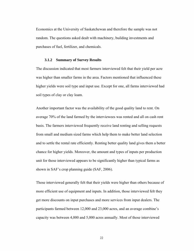
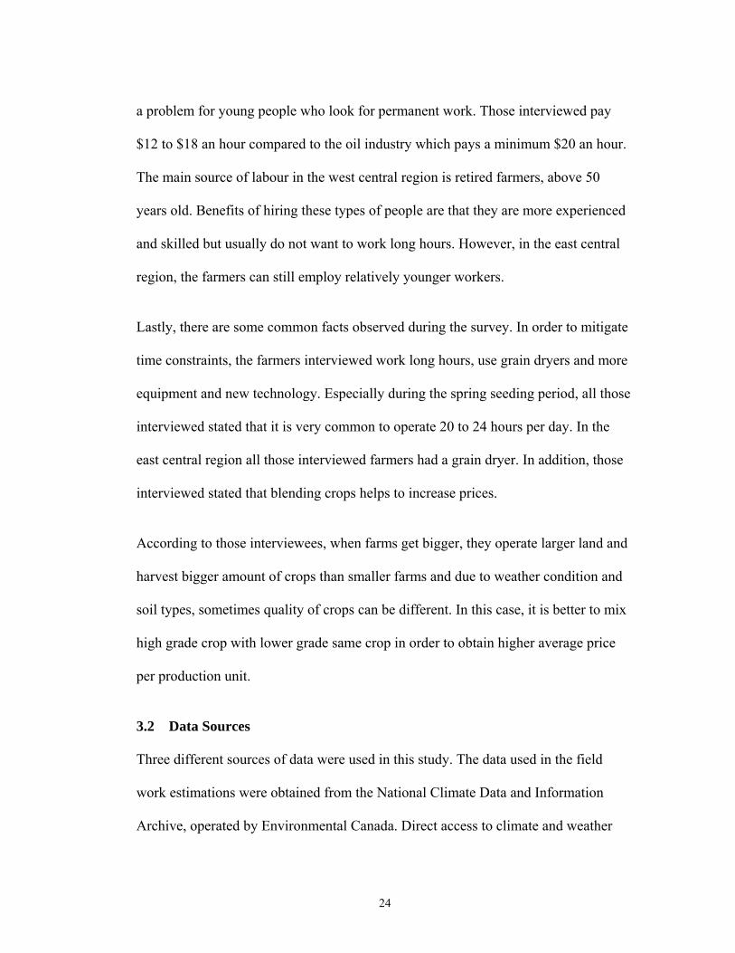
(Figure 3.4). For herbicide and fertilizer, there are some decreasing trend for farms in
the west central Saskatchewan and shows constant trend for the east central because
of weather condition and soil texture (Figure 3.5 and 3.6). There is no change in
fertilizer expense per dollar sale for the east central area.
EAST CENTRAL
WEST CENTRAL
0
5
10
15
20
25
30
0 1000 2000 3000 4000 5000 6000 7000 8000 9000 10000 11000
acre
$ per acre
Figure 3.4 Total wage per acre
28
East Central
East Central
West Central
West
0
5
10
15
20
25
30
0 1000 2000 3000 4000 5000 6000 7000 8000 9000 10000 11000
acre
$ per acre
Figure 3.5 Fertilizer expense per acre
East Central
West Central
0
5
10
15
20
25
30
0 1000 2000 3000 4000 5000 6000 7000 8000 9000 10000 11000
acre
$ per acre
Figure 3.6 Herbicide expense per acre
29

Although some expenses have direct relationships with crop acres, there are some
expenses which decrease with the increase of crop acres for the selected areas.
Because of large percentage share of fuel and repair expenses on total cost, overall
expenses per acre decrease slightly when farms grow larger. Figure 3.7 and 3.8 show
east and west central’s fuel and repair costs. For the selected areas, shares of repair
and fuel expenses on per acre show same trend. The reduction of fuel expense is
much higher for farms with up to 6,000 crop acres.
Figure 3.9 shows the relationship between farm size and machinery assets. For the
regions’ machinery assets on a per acre basis show relatively constant trend as crop
acres increase.
East Central
West Central
0
5
10
15
20
25
30
0 1000 2000 3000 4000 5000 6000 7000 8000 9000 10000 11000
acre (000)
$ per acre
Figure 3.7 Fuel expense per acre
30
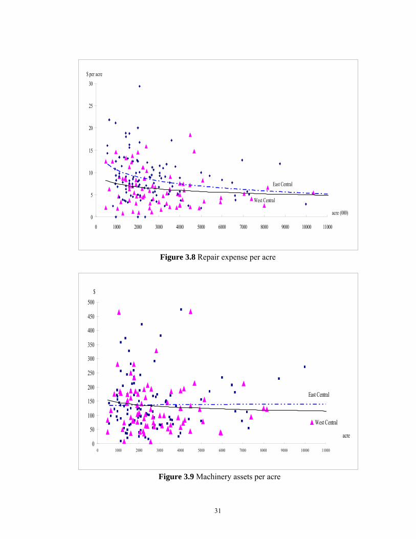
West Central
East Central
0
5
10
15
20
25
30
0 1000 2000 3000 4000 5000 6000 7000 8000 9000 10000 11000
acre (000)
$ per acre
Figure 3.8 Repair expense per acre
East Central
West Central
0
50
100
150
200
250
300
350
400
450
500
0 1000 2000 3000 4000 5000 6000 7000 8000 9000 10000 11000
acre
$
Figure 3.9 Machinery assets per acre
31

CHAPTER 4.
ANALYTICAL FRAMEWORK
This chapter presents the framework for the analysis of the crop farms in
Saskatchewan. The first section presents a description of the field workday model
including major criteria and general procedure of suitable workdays. This is followed
by the discussion of the Least-Cost approach to determine optimal size of farm
machinery.
4.1 Determination of Daily Field Workability
Machinery selection would be much easier if the number of available workdays could
be estimated with a reasonable degree of certainty. In many areas of Canada the most
critical limiting factor is the lack of field tractability at the time when either spring
planting and harvesting must be done (Dyer, 1980). The limited numbers of field
workdays can make the effective growing season shorter than the frost free period
would indicate. The expected number of workdays during a critical period, such as
harvest time, largely may determine the size of machinery needed for a given size farm.
For instance, larger or more efficient combines may be needed to complete a harvest
when work time is limited.
In spring and fall poor field work conditions occur immediately after a heavy rain and a
temperature below 0 degrees Celsius. The number of non-workdays following rain
varies with the amount of rainfall and the type of soil, since both factors influence the
time for excess soil water to drain through the top layer of soil. These two factors are
32

important for determining a field workday. In general, a field workday can be defined
as a day with no snow cover or amount of daily evaporation is more than daily rainfall.
This definition assumes that different criteria apply to different field operations.
4.1.1 The Selection of the Field Workday Model
A variety of models have been previously developed to evaluate a suitable field
workday. After reviewing soil workability models, transitional probability equations
derived from the Markov Chain method has been selected to estimate expected field
workdays. Although, the Markov Chain method oversimplifies the real conditions in
the field in this procedure, it can be useful to approximate the probability of the field
days. For most of the cases, some additional factors, operator time and machinery
availability, affect the decision of whether or not to operate machinery in a particular
field. Unfortunately, accurate information is currently not available for describing the
effects of these factors on field workdays in the study areas. Thus the only factors
used for this thesis is the tractability of soil with regard to its moisture level and soil
type.
4.1.2 Major Criteria for Soil Tractability and Field Workdays
The interaction between rainfall, evapotranspiration and soil moisture influences soil
tractability and determines the number of workdays for a specific soil, limiting time
for seeding and harvesting (Pote et al., 1997). In order to determine available field
work time, one needs to know which day is suitable for field work and what criteria is
used to determine a day is workable. This estimation only takes into account daily
precipitation and temperature due to lack of important soil moisture data.
33
Fr this paper, a day is assumed to be suitable for fall and spring field work if one of
the following criteria is met:
1) Daily precipitation is less than 2.5 mm
Such criterion is justified in areas where the average rate of evaporation exceeds 2.5
mm. When a daily rainfall of less than 2.5 mm occurs, it generally evaporates during
the day and thus can be defined as a suitable field workday (Amir et al., 1976).
2) Max air temperature was above 0 degrees Centigrade
A soil is assumed to be intractable, when temperature falls below 0 degrees
Centigrade. Above 0 degrees Centigrade, farm machines can work on soil to
satisfactory perform the function of the machine, without causing significant damage
to the crop yield or quality.
3. A day is suitable for field work if the previous two or more consecutive rainy
days’ daily precipitation does not exceed 2.5 mm (Ayres, 1975)
When two or more consecutive rainy days’ daily precipitation is greater than or equal
to 2.5 mm, then these rainy days including the next non rainy day are counted as
unsuitable for field operations.
34
4.1.3 A Procedure for Determining Probabilities of Spring and Fall Field
Workdays
The procedure described in this part uses conditional probability equations derived
from the Markov Chain method. In mathematics, a Markov chain is a discrete-time
stochastic process with Markov property (Shiryaev, 1996). A Markov chain is a series
of states of a system that has the Markov property. At each time the system may have
changed from the state it was in the moment before, or may have stayed in the same
state. The changes of state are called transitions. The series with the Markov property is
such that the conditional probability distribution of the state in the future, given the
state of the process currently and in the past, is the same distribution as one given only
in the current state (Shiryaev, 1996). Markov Chain principles previously had been
applied for determining field workday and non workday probabilities using observed
data for many locations in North America (Ayres, 1975).
The purpose of this section is to provide an applicable procedure for determining the
probabilities of field workdays when only observed data is available and verify the
resulting calculated probabilities for two locations in Saskatchewan, namely the
Kindersley and Yorkton. When daily weather data is available, the observed
probabilities of “n” (n = 1,…,i) consecutive field workdays can be estimated by using a
simple probability equation. Then based on the observed probabilities, it is possible to
come up with the calculated field workday probabilities.
The basic probability equation for determining “n” consecutive field workdays or
non-workdays is:
35

)1](/[][][ −= nSSPSPnSP ………………………………….…(4.1)
where:
P[nS] - probability of “n” consecutive S days;
n - integer, express number of consecutive days, n ≥ 1;
S - a field workday;
P[S] - probability of a single S day;
P[S/S] - conditional probability of a single S day given the previous day was also S.
In probability theory and statistics, the exponential distributions are a class of
continuous probability distributions. They are often used to model the time between
independent events that happen at a constant average rate (Shiryaev 1996). For
practical purposes, equation 4.1 has been converted into following equation (Amir,
1977).
1;][ ≥= nenSP ni
βα ……………………………………………… (4.2)
where α and β are constants to be determined for local data.
The conversion of equation (4.1) to equation (4.2) can be accomplished by (Hastie et
al., 2001):
βα eSP i =][ …………………………………………………….…….…. (4.3)
βeSSPi =]/[ …………………………………………………..………. (4.4)
36
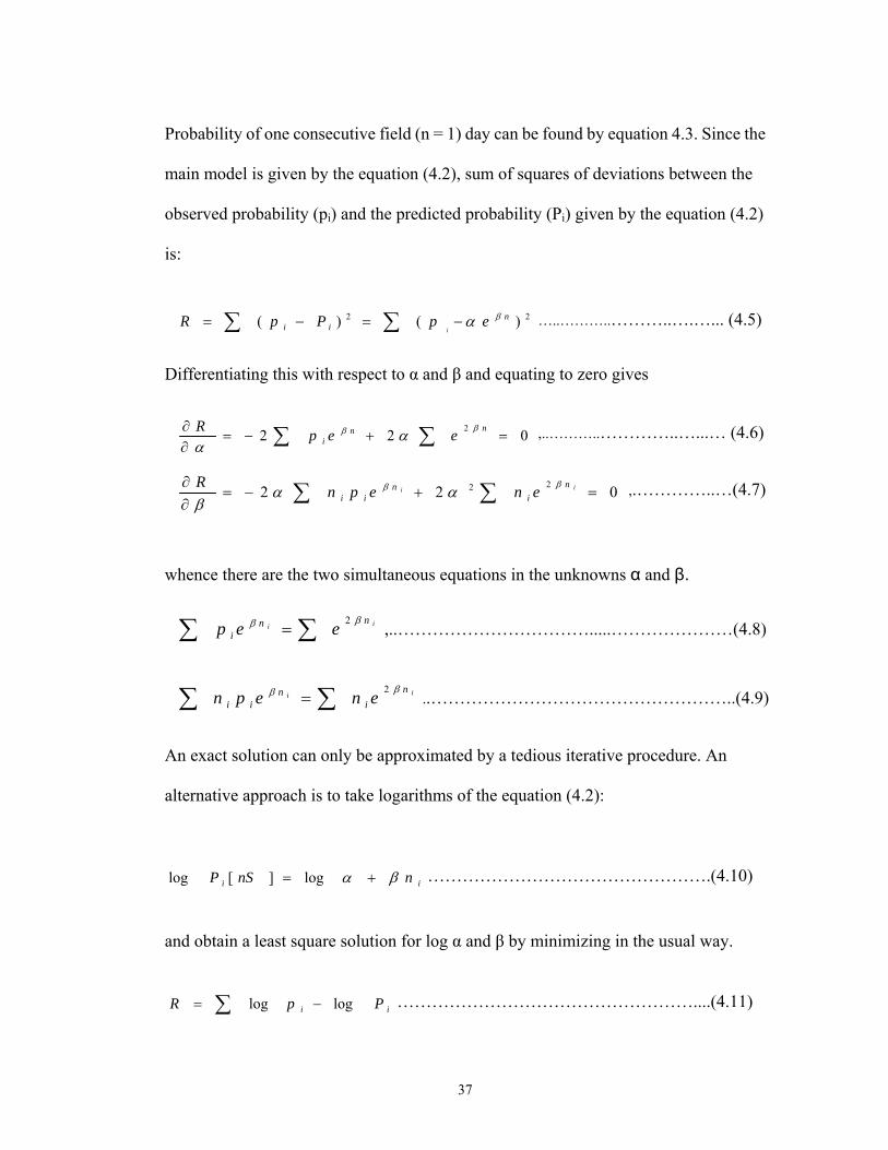
Probability of one consecutive field (n = 1) day can be found by equation 4.3. Since the
main model is given by the equation (4.2), sum of squares of deviations between the
observed probability (pi) and the predicted probability (Pi) given by the equation (4.2)
is:
22 )()( n
ii epPpRi
βα∑∑ −=−= …..………..………..….…... (4.5)
Differentiating this with respect to α and β and equating to zero gives
022 2=+−=
∂∂ ∑∑ nn
i eepR ββ αα
,..………..…………..…...… (4.6)
022 22 =+−=∂∂ ∑∑ ii
ni
nii enepnR ββ αα
β,.…………..…(4.7)
whence there are the two simultaneous equations in the unknowns α and β.
ii
nni eep ββ 2∑∑ = ,..…………………………….....…………………(4.8)
iin
in
ii enepn ββ 2∑∑ = ..……………………………………………..(4.9)
An exact solution can only be approximated by a tedious iterative procedure. An
alternative approach is to take logarithms of the equation (4.2):
ii nnSP βα += log][log ………………………………………….(4.10)
and obtain a least square solution for log α and β by minimizing in the usual way.
ii PpR loglog −= ∑ ……………………………………………....(4.11)
37
In addition, n consecutive field workdays observed probabilities (pi(nS) can be
estimated by dividing the frequencies of n consecutive field workdays for ith month
by total number of days available follows:
nyM
nDFnDpi
ii
⋅=
][][ ……………………………………………………(4.12)
where
pi[nD] – probability of n consecutive field workdays for ith month;
Fi[nD] – frequencies of n consecutive field days for the ith month;
Mi - number of days in the ith month;
y - number of observed years.
4.2 The Least-Cost Approach to Estimate the Optimal Size of Agricultural
Machinery
On today’s commercial farm, economic pressures are motivating operators to
concentrate on managing their machinery resources. The long-standing trend of
replacing capital for labour by adding higher capacity and more efficient machinery
has resulted in large amounts of capital being used annually to acquire more
machinery (Dalsted and Guitierrez, 2001). Increasing capital investment has had a
dramatic effect on production costs, labour requirements, productivity and product
quality. For instance, the increase in machinery investment can ease workers tasks
and improve labour efficiency. In addition, the use of bigger machinery has
contributed to higher machinery investment per farm and has made it possible for an
38

individual operator to farm many acres (Kay et al., 2004, pp. 402). Therefore,
effectively managing machinery investment cost is essential to minimize total
production cost.
The average annual machine costs fall in three basic categories: (1) fixed costs, (2)
variable costs, and (3) timeliness costs. The specific machinery resources of these
categories are identified briefly and characterized below.
4.2.1 Estimation of Machinery Fixed Cost
Fixed costs (FC) are those outlays that do not vary depending on machine use. There
are some terminologies commonly used interchangeably with fixed costs such as
ownership and overhead costs.
Regardless of the terminology used, fixed costs include the following items:
1. Interest expense: Investment in machinery ties up capital and should be
assigned a capital cost (Kay et al., 2004). The rate will depend on the
opportunity cost for that capital elsewhere in the farm business if the
operator uses his or her own capital. If capital is borrowed to finance the
machinery investment, that cost should be at least large enough to cover
the interest paid on the loan. When operators borrow money to invest in
machinery, lenders determine how much interest is charged. Interest rates
can fluctuate depending on the amount of money borrowed. If only part
of the money is borrowed, an average of the two rates should be used.
Choosing the interest rate is vital to calculate accurate machinery
estimates.
39
2. Depreciation - is a way of representing, how capital assets decline in
value over time because of wear and obsolescence. Hard assets, such as
machinery, depreciate over time and must eventually be replaced.
Depreciation costs need to be calculated over the estimated useful life of
the asset. In this way, the farm’s cost of capital equipment is reflected
more appropriately in the unit costs of goods produced by that farm
equipment.
The joint costs of depreciation and interest can be calculated by using a
capital recovery factor (CRF) (Hunt, 1987). Capital recovery is the
number of dollars that would have to be set aside each year to repay the
value lost due to depreciation and pay interest costs. CFR can be used to
combine the total depreciation and interest charges into a series of equal
annual payments at compound interest. These payments plus the interest
on the undepreciated amount, S, can be used to estimate the capital
consumption (CC) of farm machinery (Hunt, 1987).
1)1()1(
)(
−++
=
+−=
L
L
vvp
iiiCRF
iSCRFSPCC …………………(4.13)
where:
SV - salvage value percentage,
L - years of life.
40

3. Housing and insurance (HI): Most machinery cost estimates include an
annual cost for housing the machine and insuring it. These costs generally
are much smaller than depreciation and interest expense however; they
have to be considered carefully.
Insurance should be carried on farm machinery to allow for replacement
in case of a disaster such as a fire, collision and theft. For charge
insurance needs to be included in fixed costs because some losses can be
expected over time. If the owner decides not to purchase insurance for
machinery, the risk is assumed by the rest of the farm business (Kay et al.,
2004).
There is a variety of housing for farm machinery. Basically, providing
shelter and maintenance equipment for machinery may result in less
deterioration of mechanical parts and appearance from weathering and
fewer repairs in the field. On the other hand, fewer repairs and less
deterioration can reduce machinery repair and maintenance costs
significantly (James and Eberle, 2000). That should produce greater
reliability in the field and a higher trade-in value. The HI costs are
usually expressed as percentage of the average investment. In this study,
insurance and housing cost per year is determined as one percent of the
original cost of the machinery (SAF, A Rental and Custom Rate Guide,
2006).
41
After determining all the costs mentioned above, the estimation of the total fixed
costs can be expressed as a percent of the purchase price. The FC percentage is the
sum of capital consumption (CC from Eq 4.2) and percentage for housing and
insurance.
HISii
iiSFC vL
L
v +⋅+−+
+⋅−= )
1)1()1(()1(% …(4.14)
4.2.2 Estimation of Machinery Variable Costs
Variable costs are defined as those costs that change relative to a change in an
operational activity or business. In regards to everyday operations these are the costs
associated with inputs and services required to operate the machine. The variable
costs are also called operating costs and are measured on a per unit of production
basis such as per acre or hours of use.
The variable costs for machinery include fuel, lubrication, maintenance repairs and
operator’s labour. The correct estimation of these costs is important because some
machines will use these inputs more efficiently than others. Better technology and
quality can bring the efficiency that cuts repair requirements and energy waste.
Fuel and lubrication: The fuel cost estimation is based on the engine consumption
rate. The consumption rate can come from either performance records or engineering
equations and is based on engine size (American Society of Agricultural Engineers,
2001). Fuel cost is a function of the percent loading, fuel price and total hours of
machinery use (Brown and Schoney, 1985). Fuel cost is calculated as follows:
42
)()())(0098.020.023.2(20.1
100/)()(2 D
ii
ii PHRST
PLPLPLMaxPTOHPf ⋅⋅
⋅−⋅+⋅⋅
=
(4.15)
where:
fi – tractor fuel cost,
Max PTOHP – the size of machinery that will pull or carry all implements within
load factor of no more than 80 percent,
PL – percent load used by the ith implement,
HRST – total tractor hours,
PD – price of diesel fuel per litre.
Repair and maintenance (RM): Expenditures for parts and labour installing
replacement parts are a part of RM costs. Repair costs for farm machinery normally
go up as the use of machinery increases. Depending on field working conditions, the
repair costs required for identical machines used the same hours can be different.
Precise predictions of machinery RM costs are not easy to obtain. Thus repair and
maintenance costs are normally estimated as a constant percentage of purchase price
per hour and depend on machine type (SAF, Custom Rate Guide, 2005).
Labour cost: In the estimation of machinery variable costs, labour cost is an
important variable cost. Although labour costs are usually estimated separately from
machinery costs, it is better to be included in the given machinery variable costs.
When the machine operator is a hired worker, these costs also should be included in
43

the machinery variable costs for the farm. Labour costs are usually quoted by hours
that include time spent fuelling, lubricating, repairing, adjusting and moving
machinery between fields and working in the field.
Annual variable costs (VC) include repairs and maintenance, oil, fuel and labour are a
function of the area covered, speed of operation, field efficiency and width of the
machine (Brown and Schoney, 1985).
In the estimation of timeliness cost, area covered, speed of operation, with of
machine, field efficiency and the timeliness loss factor must be considered.
Field efficiency: In farm machinery cost estimation, one needs to obtain the
effective field capacity of the machine. The capacity of a machine is the number
of units which it can process or cover in a specific time. Capacity is expressed
as the area covered or volume harvested per unit of time. The effective field
capacity is the measure of a machines ability to do a job under actual field
conditions. To estimate effective field capacity, calculate the theoretical field
capacity and multiply by the field efficiency. Field efficiency is defined as the
percentage of time the machine operates at its full rated speed and width while
in the field.
Effective Capacity = Theoretical Field Capacity x Field efficiency
The machine cannot operate at its theoretical capacity at all times while it is in
the field due to the following factors (Hunt, 2001):
44
- Turning and idle travel
- Land topography
- Operating at less than full width
- Operator’s personal time
- Handling seed, fertilizer, chemicals, water or harvested materials
- Cleaning clogged equipment
- Machine adjustment
- Lubrication and refuelling during the day
- Waiting for other machines
- Waiting for repairs to be made.
As a result of these factors, the field efficiency is always less than 100 percent.
The VC is estimated as follows:
)])[( iiiii LwfORMewS
AcVC +⋅++⋅⋅⋅
⋅= …………(4.16)
VCi – annual variable cost implement i,
C – constant (8.25 english system),
A – area covered (acre),
S – speed of operation (mph),
e – field efficiency (%),
w – width of machine (ft),
RM – repair and maintenance cost ($/hr),
o – oil cost ($/hr),
45

f – fuel cost ($/hr) and
L – labour cost ($/hr).
4.2.3 Estimation of Timeliness costs
Timeliness costs are closely connected to machine size and do not belong to either the
fixed or variable costs. Timeliness costs increase due to the inability to complete field
tasks in a certain time period (Gunnarsson and Hansson, 2003). In some years, farm
operators could not harvest during the most appropriate period because of weather
delay. In this case, delaying harvest can cause reduction in crop quality and potential
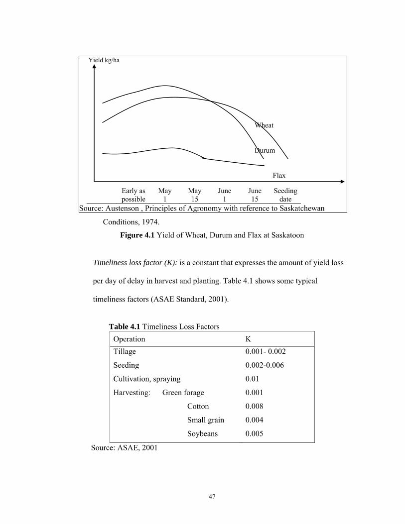
yield (Figure.4.1). For instance, “wheat has been reported to suffer a 46% reduction
in yield for each week of delay in planting” (Hunt, 2001, p. 391). Timeliness cost is
very important when farmers compare and select different sizes and capacity of
machinery.
Timeliness costs associated with undersized farm machinery can be difficult to
measure. This cost varies not only between crops but also depends on operations
completed on that crop. Timeliness costs are often identified as money value of
amount of yield reduction per day of delay.
46
Yield kg/ha
Source: Austenson , Principles of Agronomy with reference to Saskatchewan
Wheat Durum Flax
Early as possible
May 1
May 15
June 1
June 15
Seeding date
Conditions, 1974.
Figure 4.1 Yield of Wheat, Durum and Flax at Saskatoon
Timeliness loss factor (K): is a constant that expresses the amount of yield loss
per day of delay in harvest and planting. Table 4.1 shows some typical
timeliness factors (ASAE Standard, 2001).
Table 4.1 Timeliness Loss Factors Operation K Tillage
Seeding
Cultivation, spraying
Harvesting: Green forage
Cotton
Small grain
Soybeans
0.001- 0.002
0.002-0.006
0.01
0.001
0.008
0.004
0.005
Source: ASAE, 2001
47

Total timeliness costs can be defined as follow:
hDPVYK
ewSAcT i ⋅
⋅⋅⋅
⋅⋅⋅
=])[(
2………………….…….(4.17)
where:
Ti –timeliness cost of implement I ($/yr),
K – timeliness loss factor (K=0.004 for small grain),
Y – potential crop yield,
A – crop area (acre),
W – width of machine,
e – field efficiency,
V – value of crop,
P[D] – probability of a given operation’s field workday,
h – total work hours available per day.
4.2.4 Estimation of the Least-Cost Size of Machinery
An optimal machinery system is important for farming to be economically
competitive. For crop farming in Saskatchewan, the combine harvester is the most
important machine. Although the farm machinery used in spring planting is also very
important, seeding capacity of machinery is usually much higher than combine
capacity. In addition, the combining is the most expensive and time consuming
operation on the farm. Therefore, minimizing the total cost for the harvest operation
can be one of the key elements for crop production to improve efficiency.
48
To attain high yields of good quality there are optimal times for performing field
operations for crop production (Witney, 1996). Related to optimal times for field
operations, optimizing machinery size is one of the important factors for farm
profitability. The optimizing machinery size can be achieved by minimizing
machinery costs for a given farm operation. The minimizing machinery cost
procedure described in the following section is based on Brown and Schoney’s
(1985) paper.
The least-cost procedure is divided into two stages. In stage 1, total combine costs are
defined. for variety types of combines.
)])[(100
%)(iiiii
ii LwfORM
ewSAcwpFCTC +⋅++⋅⋅⋅ i
⋅+
⋅⋅=
(4.18)
where i implies ith type of machinery.
Calculating the least cost size of combine, one needs to consider a variety of factors
such as soil textures, weather condition, crop types and yield.
Minimizing machinery total cost with respect to width of machinery defines
minimum cost represented by Equation 4.18,
eSpFCLAcw⋅⋅⋅
⋅⋅⋅=
%)(100 ………………………………………………...4.19
49

Including the charge for timeliness, Equation 4.19 can be modified;
⎟⎟⎠
⎞⎜⎜⎝
⎛⋅⋅⋅⋅
+⋅⋅⋅⋅
⋅⋅=
hDPAVYKL
eSpFCAcw l ])[(%)(
100 ,……...(4.20)
where:
p – purchase price of machinery,
wl – the least cost width of machinery.
The machine width, wl, found by this procedure, represents the width consistent with
a least cost combine. The total least cost machinery width for combines depends on
what class of combine is employed for a given farm. If an operator uses larger size
and big capacity combine, the least cost size of combine can be shorter than small
combines if the farmer uses in his or her operation. On the other hand, the least-cost
estimation can be based on size of crop acres. It can give an opportunity to determine
combine’s the most efficient use of crop acres. Therefore, the estimation of least cost
size of combine requires careful consideration.
On the other hand, farm operators usually use the same types of combine with the
same width. In this case, the least cost acre a combine can be derived from Equation
4.20 with respect to crop area (Appendix 4).
50

CHAPTER 5.
RESULTS OF COMBINE CAPACITY
This chapter reports and interprets the result of the analysis that were undertaken to
examine the amount of crop area combine per year and the effect of combine cost on
production cost for the selected areas. In the estimation of the combine capacity, fall
field workdays and optimal acre per combine were determined. It is followed by the
comparison results between farms in the west and east central regions.
5.1 Estimated Result for Fall Field Workdays
In farm machinery planning, knowledge of suitable field work time is one of the
important factors to consider both for spring planting and fall harvesting. Based on
the estimation of available field work time, one can determine how much time is
available for harvesting and can make decisions on sizes of machines or systems of
machines needed for the farm operation or calculate the amount of area that can be
done by a particular size of machine. The determination of available total time during
the harvest period followed the certain steps which were explained in Chapter 4.
The model described in Chapter 4 was used to determine the probability of spring and
fall field workdays on a monthly basis, August and September, using the previous 25
years of weather records in the both west and east central Saskatchewan. Due to
weather dissimilarity between these areas, the probabilities of field workdays in the
west central Saskatchewan are higher than the east central Saskatchewan. The results
will be explained in the following sections. The results of the calculated probabilities
51
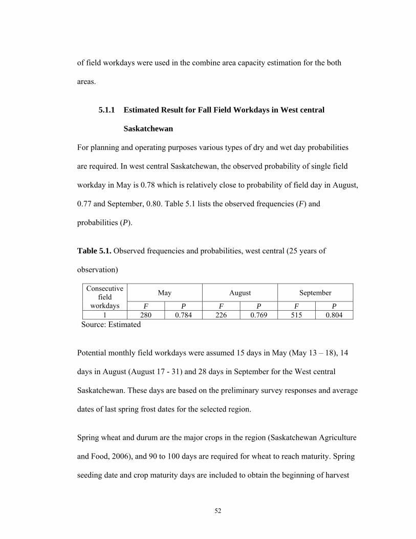
of field workdays were used in the combine area capacity estimation for the both
areas.
5.1.1 Estimated Result for Fall Field Workdays in West central
Saskatchewan
For planning and operating purposes various types of dry and wet day probabilities
are required. In west central Saskatchewan, the observed probability of single field
workday in May is 0.78 which is relatively close to probability of field day in August,
0.77 and September, 0.80. Table 5.1 lists the observed frequencies (F) and
probabilities (P).
Table 5.1. Observed frequencies and probabilities, west central (25 years of
observation)
May August September Consecutive field
workdays F P F P F P 1 280 0.784 226 0.769 515 0.804
Source: Estimated
Potential monthly field workdays were assumed 15 days in May (May 13 – 18), 14
days in August (August 17 - 31) and 28 days in September for the West central
Saskatchewan. These days are based on the preliminary survey responses and average
dates of last spring frost dates for the selected region.
Spring wheat and durum are the major crops in the region (Saskatchewan Agriculture
and Food, 2006), and 90 to 100 days are required for wheat to reach maturity. Spring
seeding date and crop maturity days are included to obtain the beginning of harvest
52

date. In the estimation, August 17 was assumed to be the beginning of harvest date
due to crop maturity period for the west central Saskatchewan. In addition, analysing
the previous 25 years weather data shows that daily temperature usually drops below
0 degrees Centigrade after September 28 which reduces the time available for
harvesting.
5.1.2 Estimated Result for Fall Field Workdays in East central
Saskatchewan
In the east central region of Saskatchewan, the observed probability of single field
workday in May is 0.80 which is relatively higher than probability of field day in
August, 0.72 and September, 0.77. Thus, the observed probability of 1 consecutive
dry day is 0.72. Table 5.2 lists the observed frequencies (F) and probabilities (P).
Table 5.2 Observed frequencies and probabilities, East central (24 years of
observation)
May August September Consecutive field
workdays F P F P F P 1 601 0.808 209 0.726 576 0.773
Source: Estimated
The potential monthly field workdays were assumed to be the same as the west
central Saskatchewan, 15 days in May (May 13 – 18), 14 days in August (August 17 -
31) and 28 days in September for the east central Saskatchewan. The first killing frost
occurs after September 10th in east central and the average frost-free period is around
109 days. Thus, there is enough time for crops to reach maturity for the east central
53

Saskatchewan. Canola and spring wheat are the major crops in the region
(Saskatchewan Agriculture and Food, 2006). The same procedure followed for west
central Saskatchewan part was used in the estimation of field workdays in this region.
5.2 Estimated Result for the Optimal Area Combined
The cost of every class of combine is different because the price of combine, power,
energy consumption and size of header are different. Since a different combine uses a
different size of header, determining the optimal size of combine is difficult to
estimate. To simplify this, in the machinery cost estimation, cost of a “class 7”
combine was determined separately for both regions and compared to each other. In
addition, the preliminary survey found that larger farms in both areas mainly use
“class 7” combines with 40 ft header. The total cost of a “class 7” combine was
estimated with or without custom work for 5,000 acres to 25,000 acres.
5.2.1 Optimal Area Combined in the West central Saskatchewan
The estimated results of every thousand acres for fall harvest machinery costs with or
without custom work for 5000 acres to 25000 acres assuming that operators use
“class 7” combines with 40 ft header during the harvest period are shown in Figure
5.1. From the machinery costs estimation, a “class 7” combine can harvest around
4974 acres in the west central Saskatchewan during the giving period of August 17 to
September 28 which was around 33 field workdays according to the field workday
estimation. It suggests that when crop area increases every 4,974 acres for west
central Region, a “class 7 “ combine costs are minimized. For instance, when an
operator of farm uses only one “class 7” combine in his or her operation in this area,
54
least cost operational acres would be 4974 acres and costs $18.47 per acre. For 2
combines, 9,948 acres would be the most optimal operational acres. Table 5.3 shows
the estimation total combine costs.
In addition, between combine units total costs may go up quickly as a result of rising
timeliness costs. From the results, crop acres above combine capacity have caused
quick increases in timeliness cost for example, 5,000 acres to 8,000 acres. When crop
acres reach 7,000, the result suggests that it is the right decision to purchase a second
combine. Two combines cost $24.06 per acre for 7,000 acres which is much lower
than using only one combine (Table 5.3). The trend can be seen graphically in Figure
5.1 which shows when a farm owner needs to purchase the next combine.
Figure 5.2 shows minimum total combine cost if farmers use different types of
combines, such as class 5 combine with 20 ft header, class 7 combine with 40 ft
header and class 8 combine with 42 ft header. In this estimation “class 8” combine
was assumed to have a higher working speed, (6 mph) and 10 % higher purchase
price and costs. In the west central Saskatchewan, the estimated optimal capacity of
combine were 1866 acre for class 5 and 7832 acre for class 8 combine (Figure 5.2).
The results showed that it is better to purchase a larger combine, when farmers
operate above 3000 acres. As well, using a “class 8” combine can be more efficient
above 4974 acres.
55

56
(TC – total cost, FC – fixed cost, OC – operation cost, Ti – timeliness cost, Cu custom cost and TCc – total costs with custom work)
0
5
10
15
20
25
30
35
5 6 7 8 9 10 11 12 13 14 15 16 17 18 1
$
9 20 21 22 23 24 25
acre (000)
TCFCOCTi TCcCu
0
10
20
30
40
50
60
70
80
90
1 2 3 4 5 6 7 8 9 1 1 1 1 1 1 1 1 1 1 2 acres (000)
$
Figure 5.1 Machinery cost per acre, west central Region
TC5TC7TC8
Figure 5.2 Minimum total combine cost for class 5, 7 and 8.

57
Table 5.3 Machinery cost per acre for 5,000 acres to 25,000 acres, west central Region (Field efficiency – 0.8)
Number of
combine
Crop acre
TC per acre no custom
FC per acre
VC per acre
Ti cost
TC per acre with
custom
Custom cost
Number of
combine
Crop acre TC per acre no custom
FC per acre
VC per acre
Ti Cost
TC per acre with
custom
Custom cost
1 4974 18.47 13.29 5.18 0.00 18.47 0.00 3 15000 18.83 13.22 5.18 0.43 18.58 0.092 5000 18.83 13.22 5.18 0.43 18.58 0.09 4 15000 22.80 17.62 5.18 0.00 22.80 0.001 6000 30.39 11.01 5.18 14.19 22.10 3.06 3 16000 23.16 12.39 5.18 5.59 19.90 1.212 6000 27.21 22.03 5.18 0.00 27.21 0.00 4 16000 21.70 16.5.2 5.18 0.00 21.70 0.001 7000 38.64 9.44 5.18 24.02 24.61 5.19 4 17000 20.73 15.55 5.18 0.00 20.73 0.002 7000 24.06 18.88 5.18 0.00 24.06 0.00 5 17000 24.62 19.43 5.18 0.00 24.62 0.001 8000 44.84 8.26 5.18 31.39 26.50 6.78 4 18000 19.87 14.68 5.18 0.00 19.87 0.002 8000 21.70 16.52 5.18 0.00 21.70 0.00 5 18000 23.5.2 18.35 5.18 0.00 23.5.2 0.003 8000 29.96 24.78 5.18 0.00 29.96 0.00 3 19000 33.43 10.43 5.18 17.81 23.02 3.851 9000 49.65 7.34 5.18 37.13 27.97 8.02 4 19000 19.09 13.91 5.18 0.00 19.09 0.002 9000 19.87 14.68 5.18 0.00 19.87 0.00 5 19000 22.57 17.39 5.18 0.00 22.57 0.003 9000 27.21 22.03 5.18 0.00 27.21 0.00 4 20000 18.83 13.22 5.18 0.43 18.58 0.091 10000 5.2.51 6.61 5.18 41.72 29.14 9.01 5 20000 21.70 16.52 5.18 0.00 21.70 0.002 10000 18.83 13.22 5.18 0.43 18.58 0.09 4 21000 22.13 12.59 5.18 4.36 19.58 0.943 10000 25.01 19.82 5.18 0.00 25.01 0.00 5 21000 20.92 15.73 5.18 0.00 20.92 0.002 11000 25.13 12.01 5.18 7.94 20.50 1.71 4 22000 25.13 12.01 5.18 7.94 20.50 1.713 11000 23.20 18.02 5.18 0.00 23.20 0.00 5 22000 20.20 15.02 5.18 0.00 20.20 0.003 12000 21.70 16.52 5.18 0.00 21.70 0.00 4 23000 27.87 11.49 5.18 11.20 21.33 2.424 12000 27.21 22.03 5.18 0.00 27.21 0.00 5 23000 19.55 14.36 5.18 0.00 19.55 0.003 13000 20.43 15.25 5.18 0.00 20.43 0.00 4 24000 30.39 11.01 5.18 14.19 22.10 3.064 13000 25.51 20.33 5.18 0.00 25.51 0.00 5 24000 18.95 13.77 5.18 0.00 18.95 0.003 14000 19.34 14.16 5.18 0.00 19.34 0.00 4 25000 32.39 10.57 5.18 16.94 22.50 3.664 14000 24.06 18.88 5.18 0.00 24.06 0.00 5 25000 18.5.2 13.22 5.18 0.43 18.27 0.09
Source: Estimation

A solution for keeping total combine cost lower will be to hire custom work and to
expand combine capacity. For instance, the combination of owning one combine and
hiring custom work is better for up to 7,000 acres. When crop acres exceed 8,000 acres,
purchasing a second combine will keep the machinery cost lower than hiring custom
work, as can be seen in Figure 5.1. However, combine fixed costs reach the lowest point
in 6,000, 11,000, 16,000 and 21,000 acres based on the every 1,000 acres estimation, if a
farm do not hire custom work, total machinery costs peak at the highest point due to high
cost of timeliness. Conversely, hiring custom work can reduce total cost significantly.
5.2.2 Optimal Area Combined in the East central Saskatchewan
The same procedure was followed in the estimation of combine costs for east central
Saskatchewan. During the harvest period, a “class 7” combine can harvest around 4,529
acres in this area (Table 5.4). It suggests that when crop area increases every 4,529 acres
for the East central, a regular new “class 7” combine will be needed. For instance, a
“class 7” combine costs $19.77 per acre for 4,529 acres. For 2 combines, 9,058 acres
would be the most optimal operational acres. Table 5.4 shows the estimation total
combine costs.
From the results, crop acres above combine capacity have caused a quick increase in
timeliness costs 5,000 acres to 6,000 acres. When crop acres reach 7,000 acres, the result
suggests that it is the right decision to purchase second “class 7” combine. Two combines
cost $24.8 per acre for 7,000 acres which is much lower than using only one class
combine (Table 5.4). A similar trend can be seen in Figure 5.3. The regarding to
machinery cost estimation on every 1,000 acres, when crop acres reach 12,000, 16,000
58
59
and 20,000 acres, a farm owner needs next combine to purchase. Detailed estimation of
machinery cost is shown in Table 5.4.
In the east central region, keeping total machinery costs lower will be to hire custom
work when crop acres are higher than combine capacity, especially crop acre ranges
between 5,000 to 6,000 acres, 10,000 to 11,000 acres and 14,000 to 15,000 acres (Figure
5.3). In addition, when crop area varies between 7,000 to 9,000 acres, 12,000 acres and
16,000 to 18,000 acres, extending capacity costs relatively lower than hiring custom
work. For example, the combination of owning one combine and hiring custom work is
better for up to 7,000 acres. When crop acres exceed 7,000 acres, purchasing a second
combine keeps machinery cost lower than hiring custom work, as can be seen in Figure
5.3. Although, machinery fixed costs reach the lowest point $11.01 in 6,000, 11,000 and
15,000 acres, if a farm does not hire custom work, total machinery costs peak the highest
point due to the high cost of timeliness. On the other hand, hiring custom work can
reduce total machinery cost significantly such as from $36.09 acre to $25.16 acre at 6,000
acres, $31.73 acre to $23.86 acre in 11,000 acres and $26.50 to $22.30 in 15000 acres
(Figure 5.3). Thus, the decision involved with custom hiring and purchasing new
combine requires careful consideration for farmers.
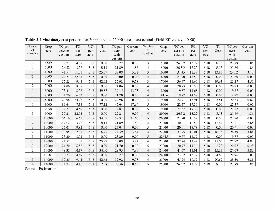
60
Table 5.4 Machinery cost per acre for 5000 acres to 25000 acres, east central (Field Efficiency – 0.80) Number
of combine
Crop acre
TC per acre no custom
FC per acre
VC per acre
Ti cost
TC per acre with
custom
Custom cost
Number of
combine
Crop acre
TC per acre no custom
FC per acre
VC per acre
Ti Cost
TC per acre with
custom
Custom cost
1 4529 19.77 14.59 5.18 0.00 19.77 0.00 3 15000 26.5.2 13.22 5.18 8.13 21.89 1.86 1 5000 26.52 13.22 5.18 8.13 21.89 1.86 4 15000 26.5.2 13.22 5.18 8.13 21.89 1.86 1 6000 41.57 11.01 5.18 25.37 27.09 5.82 3 16000 31.45 12.39 5.18 13.88 23.5.2 3.18 2 6000 27.21 22.03 5.18 0.00 0.00 0.00 4 16000 21.70 16.52 5.18 0.00 21.70 0.00 1 7000 57.25 9.44 5.18 42.62 32.92 9.78 3 17000 36.47 11.66 5.18 19.63 25.27 4.50 2 7000 24.06 18.88 5.18 0.00 24.06 0.00 4 17000 20.73 15.55 5.18 0.00 20.73 0.00 1 8000 73.31 8.26 5.18 59.87 39.15 13.73 4 18000 19.87 14.68 5.18 0.00 19.87 0.00 2 8000 21.70 16.52 5.18 0.00 21.70 0.00 4 18116 19.77 14.59 5.18 0.00 19.77 0.00 3 8000 29.96 24.78 5.18 0.00 29.96 0.00 4 19000 22.91 13.91 5.18 3.81 20.73 0.87 1 9000 89.64 7.34 5.18 77.12 45.64 17.69 5 19000 22.57 17.39 5.18 0.00 22.57 0.00 1 9058 19.77 14.59 5.18 0.00 19.87 0.00 5 19000 22.57 17.39 5.18 0.00 22.57 0.00 3 9000 27.21 22.03 5.18 0.00 27.21 0.00 4 20000 26.5.2 13.22 5.18 8.13 21.89 1.86 1 10000 106.16 6.61 5.18 94.37 52.31 21.65 5 20000 21.70 16.52 5.18 0.00 21.70 0.00 2 10000 26.5.2 13.22 5.18 8.13 21.89 1.86 4 21000 30.21 12.59 5.18 12.44 23.11 2.85 3 10000 25.01 19.82 5.18 0.00 25.01 0.00 5 21000 20.91 15.73 5.18 0.00 20.91 0.00 2 11000 33.95 12.01 5.18 16.75 24.39 3.84 4 22000 33.95 12.01 5.18 16.75 24.39 3.84 3 11000 23.20 18.02 5.18 0.00 23.20 0.00 5 22645 19.77 14.59 5.18 0.00 19.77 0.00 2 12000 41.57 11.01 5.18 25.27 27.09 5.82 4 23000 37.74 11.49 5.18 21.06 25.72 4.83 3 12000 21.70 16.52 5.18 0.00 21.70 0.00 5 23000 20.77 14.36 5.18 1.23 20.07 0.28 2 13000 49.35 10.17 5.18 34.00 29.95 7.80 4 24000 41.57 11.01 5.18 25.27 27.09 5.82 3 13587 19.77 14.59 5.18 0.00 19.77 0.00 5 24000 23.62 13.77 5.18 4.68 20.96 1.07 3 14000 57.25 9.44 5.18 42.62 32.92 9.78 4 25000 45.24 10.57 5.18 29.69 28.50 6.81 4 14000 21.72 14.16 5.18 2.38 20.36 0.55 5 25000 26.5.2 13.22 5.18 8.13 21.89 1.86
Source: Estimation
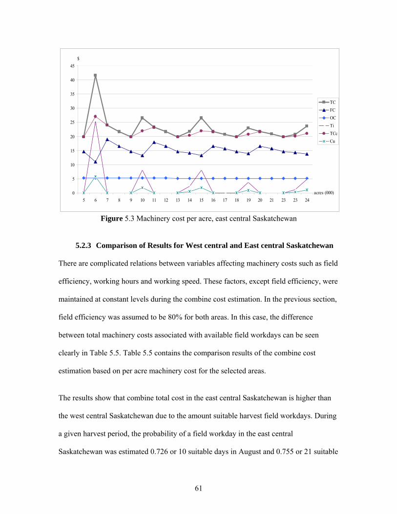
0
5
10
15
20
25
30
35
40
45
5 6 7 8 9 10 11 12 13 14 15 16 17 18 19 20 21 23 23 24 acres (000)
$
TCFCOCTi TCcCu
Figure 5.3 Machinery cost per acre, east central Saskatchewan
5.2.3 Comparison of Results for West central and East central Saskatchewan
There are complicated relations between variables affecting machinery costs such as field
efficiency, working hours and working speed. These factors, except field efficiency, were
maintained at constant levels during the combine cost estimation. In the previous section,
field efficiency was assumed to be 80% for both areas. In this case, the difference
between total machinery costs associated with available field workdays can be seen
clearly in Table 5.5. Table 5.5 contains the comparison results of the combine cost
estimation based on per acre machinery cost for the selected areas.
The results show that combine total cost in the east central Saskatchewan is higher than
the west central Saskatchewan due to the amount suitable harvest field workdays. During
a given harvest period, the probability of a field workday in the east central
Saskatchewan was estimated 0.726 or 10 suitable days in August and 0.755 or 21 suitable
61

days in September which were 2 field days lower than the west central Region. Total
combine cost per acre differs significantly because of these differences. For instance, the
estimated optimal total combine cost is $21.89 per acre for 5,000 acres in the East central
Saskatchewan which is $3.31 higher than $18.58 per acre in the West central
Saskatchewan (Table 5.5). In addition, it has to be mentioned that due to excess capacity
of combines for both areas, the estimated combine cost per acre is equal to each other
(Table 5.5). Excess power of farm machinery can provide operators to complete field
tasks reasonably short period of time. An increase in daily effective machinery capacity
had a lower effect on timeliness costs. On the other side, very low daily effective field
capacity also can lead to peculiar effects on timeliness costs.
Table 5.5 Least-cost acre for “class 7” combine
Min cost per acre
Min cost per acre
Crop acre
Number of
combine West East
Difference Crop acre
Number of
combine West East
Difference
5000 1 18.58 21.89 3.31 16000 4 21.70 21.7 0 6000 1 22.10 27.09 4.99 17000 4 20.73 20.73 0
7000 2 24.06 24.06 0 18000 4 19.87 19.87 0 8000 2 21.70 21.7 0 19000 4 19.09 20.73 1.64 9000 2 19.87 19.87 0 20000 4 18.58 21.7 3.12
10000 2 18.58 21.89 3.31 21000 5 19.58 20.91 1.33 11000 2 20.50 23.2 2.7 22000 5 20.02 20.2 0.18 12000 3 21.70 21.7 0 23000 5 19.55 20.07 0.5.2 13000 3 20.43 20.43 0 24000 5 18.95 20.96 1.12 14000 3 19.34 20.36 1.02 25000 5 18.27 15000 4 18.5.2 21.89 3.35
Source: Estimation
Besides that, the study found that field efficiency (FE) in East central Saskatchewan is
expected to be lower than the West central Saskatchewan. In the West central
Saskatchewan, the land surface is relatively smoother, flatter and with less trees than East
central Saskatchewan. In order to find the effect of FE on combine costs in this region,
62

combine costs were estimated assuming the FE is 0.75 and 0.80. The results show that
lower FE increases total combine cost. For instance, a 5 percent reduction of FE in the
East central Saskatchewan increases machinery cost per acre by $0.34 to $2.81 (1.7% -
12.84%) (Table 5.6). With the reduction of FE, the farm requires more capacity to
complete harvest. Thus field efficiency has an influence on machinery variable cost per
acre and custom hired work to increase significantly. Appendix 3 contains complete
results of combine costs estimation due to change in field efficiency.
Table 5.6 Total combine cost for East central Saskatchewan (FE =0.8 vs 0.75)
Min cost per acre
Min cost per acre
Crop acre
Number of
combine FE 0.80
FE 0.75
Difference Crop acre
Number of
combine FE 0.8
FE 0.75
Difference
5000 1 21.89 24.7 -2.81 15000 4 21.89 24.7 -2.81 6000 1 27.09 27.55 -0.46 16000 4 21.7 22.05 -0.35
7000 2 24.06 24.41 -0.35 17000 4 20.73 21.08 -0.35 8000 2 21.7 22.05 -0.35 18000 4 19.87 20.21 -0.34 9000 2 19.87 20.21 -0.34 19000 4 20.73 22.92 -2.19
10000 2 21.89 24.7 -2.81 20000 4 21.7 22.05 -0.35 11000 2 23.2 23.55 -0.35 21000 5 20.91 21.26 -0.35 12000 3 21.7 22.05 -0.35 22000 5 20.2 20.55 -0.35 13000 3 20.43 20.78 -0.35 23000 5 20.07 22.69 -2.62 14000 3 20.36 23.01 -2.65 24000 5 20.96 23.67 -2.71
Source: Estimation
When field efficiency is assumed to be 0.75 in the East central Saskatchewan, the least
cost operation acre is 4,246 acres for one combine and costs $18.75 per acre which is
$0.35 higher than when FE is 0.80 (Appendix 3). As can be seen from Table 5.6, change
in field efficiency could affect the least cost acres. However, lowering FE increases total
cost of machinery; the least-cost acres are still the same as 9,000 and 18,000 acres for the
east central area.
63

5.3 Comparison Between the Two Regions of the Farms Interviewed
The purpose of this part was to evaluate the effect of variable expenses on combine costs
and combine costs on farm production costs in both regions. The selected farms operate
14,000 acres in the West central area and 22,000 acres in the East central area were
selected and both mainly produce direct seeded spring wheat. Production costs of these
farms were estimated using the Saskatchewan Agriculture and Food, Crop Planning
Guide, 2006 (SAF, 2006 a).
According to the combine cost estimation, owning 3 “class 7” combines minimize total
fall harvest machinery costs for 14,000 crop acres in the West central region. The
estimated total rotational expense for this farm is $133.38 per acre (SAF, 2006 b).
Combining cost is $19.34 per acre (Table 5.3) which is comparatively lower than other
options of combine cost for this area. The percentage share of combine cost is equal to
15% of total production expense per acre (Figure 5.4). On the other side, 85% percent of
total farm expenses are connected with spring and summer field operations, such as
spring seeding, fertilizer, herbicide, interest and other costs.
For this farm, there can be some possibilities to decrease combine costs if the owner of
farm decide to increase operation land. However, increasing the land base requires more
machinery capacity; the cost of 3 combines can reached a minimum point when the farm
operates 14934 acres and it may reduce combine cost by $0.87 per acre.
64
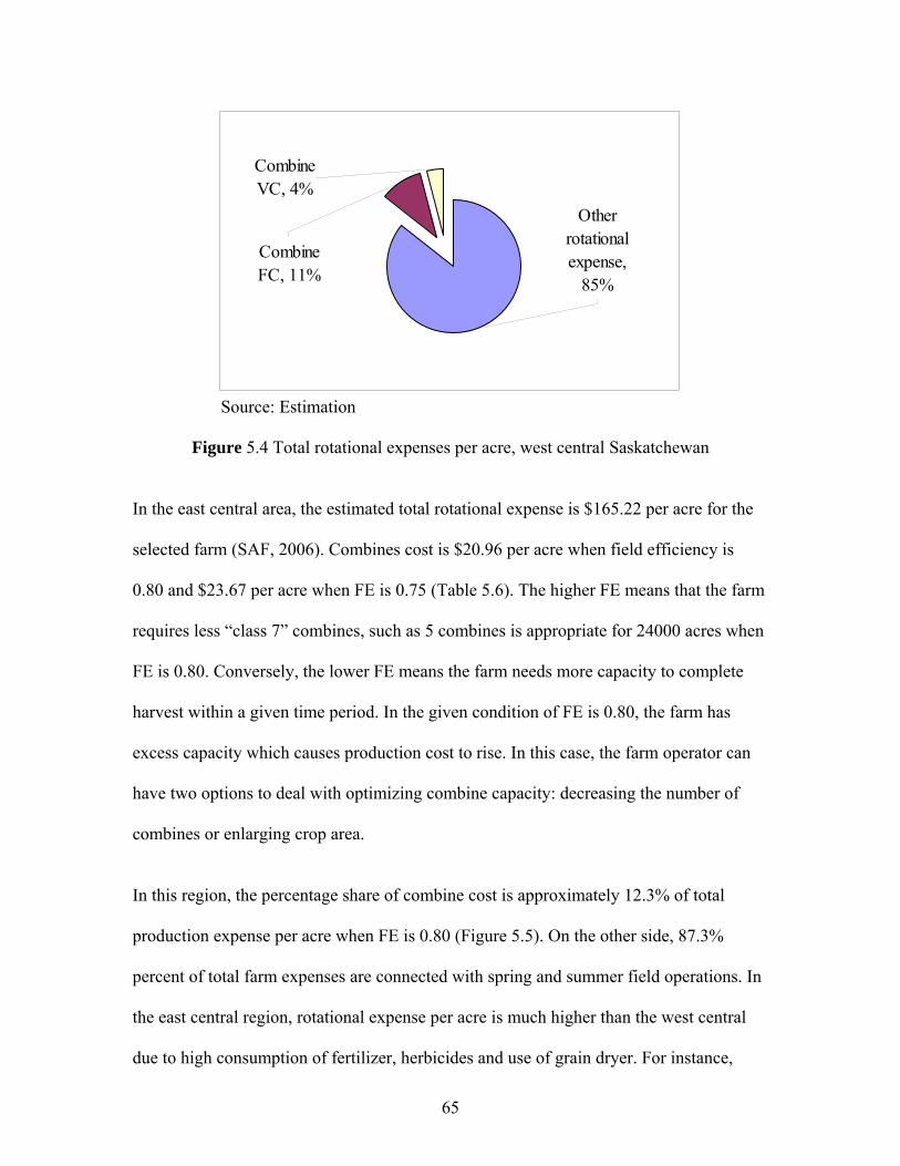
Otherrotationalexpense,
85%
CombineFC, 11%
CombineVC, 4%
Source: Estimation
Figure 5.4 Total rotational expenses per acre, west central Saskatchewan
In the east central area, the estimated total rotational expense is $165.22 per acre for the
selected farm (SAF, 2006). Combines cost is $20.96 per acre when field efficiency is
0.80 and $23.67 per acre when FE is 0.75 (Table 5.6). The higher FE means that the farm
requires less “class 7” combines, such as 5 combines is appropriate for 24000 acres when
FE is 0.80. Conversely, the lower FE means the farm needs more capacity to complete
harvest within a given time period. In the given condition of FE is 0.80, the farm has
excess capacity which causes production cost to rise. In this case, the farm operator can
have two options to deal with optimizing combine capacity: decreasing the number of
combines or enlarging crop area.
In this region, the percentage share of combine cost is approximately 12.3% of total
production expense per acre when FE is 0.80 (Figure 5.5). On the other side, 87.3%
percent of total farm expenses are connected with spring and summer field operations. In
the east central region, rotational expense per acre is much higher than the west central
due to high consumption of fertilizer, herbicides and use of grain dryer. For instance,
65

$20.70 fertilizer cost per acre in brown soil is much lower than $27.60 per acre in black
soil (Crop Planning Guide, 2006). As well, the farmers interviewed said that it is very
common to use a grain dryer in their operation in the East central due to weather
conditions. According to the Crop Planning Guide, using a grain dryer increases
production expense by $0.70 per acre.
Customhired, 1.2%
Otherrotationalexpense,87.5%
CombineFC, 8.3%
CombineVC, 3.1%
Source: Estimation
Figure 5.5 Total rotational expenses per acre, East central Saskatchewan
Due to lack of data availability, the economies of size for crop farms were difficult to
determine. Most participants, in the 2005, Farm Financial Survey operate less than 6,000
acres. Those farmers interviewed in the preliminary survey stated that larger farms are
able to capture discounts on variable costs such as fuel, fertilizer and chemicals especially
for fuel; discount on price may be up to 15 %.
In the combine cost estimation, major variable expenses include fuel, repair, oil and
labour costs. According to the combine cost estimation, approximately 28% of total cost
66
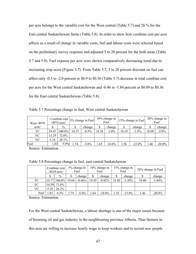
per acre belongs to the variable cost for the West central (Table 5.7) and 26 % for the
East central Saskatchewan farms (Table 5.8). In order to show how combine cost per acre
affects as a result of change in variable costs, fuel and labour costs were selected based
on the preliminary survey response and adjusted 5 to 20 percent for the both areas (Table
5.7 and 5.8). Fuel expense per acre were shown comparatively decreasing trend due to
increasing crop acres (Figure 3.7). From Table 5.7, 5 to 20 percent discount on fuel can
affect only -0.5 to -2.0 percent or $0.9 to $0.36 (Table 5.7) decrease in total combine cost
per acre for the West central Saskatchewan and -0.46 to -1.84 percent or $0.09 to $0.36
for the East central Saskatchewan (Table 5.8).
Table 5.7 Percentage change in fuel, West central Saskatchewan
Combine cost /4974 acre/
5% change in Fuel 10% change in Fuel 15% change in Fuel 20% change in
Fuel West /4974 acre/ $ % $ change $ change $ change $ change TC 18.47 100.0% 18.37 -0.5% 18.28 -1.0% 18.19 -1.5% 18.09 -2.0% FC 13.29 72.0% VC 5.18 28.1%
Fuel 1.83 9.9% 1.74 -5.0% 1.65 -10.0% 1.56 -15.0% 1.46 -20.0% Source: Estimation Table 5.8 Percentage change in fuel, east central Saskatchewan
Source: Estimation
Combine cost /4529 acre/
5% change in Fuel
10% change in Fuel
15% change in Fuel 20% change in Fuel
$ % $ change $ change $ change $ change TC 19.77 100.0% 19.68 -0.46% 19.59 -0.92% 19.50 -1.38% 19.40 -1.84% FC 14.59 73.8% VC 5.18 26.2%
Fuel 1.83 9.3% 1.74 -5.0% 1.64 -10.0% 1.55 -15.0% 1.46 -20.0%
For the West central Saskatchewan, a labour shortage is one of the major issues because
of booming oil and gas industry in the neighbouring province Alberta. Thus farmers in
this area are willing to increase hourly wage to keep workers and to recruit new people
67
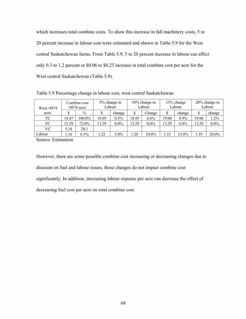
which increases total combine costs. To show this increase in fall machinery costs, 5 to
20 percent increase in labour cost were estimated and shown in Table 5.9 for the West
central Saskatchewan farms. From Table 5.9, 5 to 20 percent increase in labour can affect
only 0.3 to 1.2 percent or $0.06 to $0.23 increase in total combine cost per acre for the
West central Saskatchewan (Table 5.9).
Table 5.9 Percentage change in labour cost, west central Saskatchewan
Source: Estimation
Combine cost /4974 acre/
5% change in Labour
10% change in Labour
15% change Labour
20% change in Labour West /4974
acre/ $ % $ change $ Change $ change $ change TC 18.47 100.0% 18.89 0.3% 18.95 0.6% 19.00 0.9% 19.06 1.2% FC 13.29 72.0% 13.29 0.0% 13.29 0.0% 13.29 0.0% 13.29 0.0% VC 5.18 28.1
Labour 1.16 6.3% 1.22 5.0% 1.28 10.0% 1.33 15.0% 1.39 20.0%
However, there are some possible combine cost increasing or decreasing changes due to
discount on fuel and labour issues, these changes do not impact combine cost
significantly. In addition, increasing labour expense per acre can decrease the effect of
decreasing fuel cost per acre on total combine cost.
68

CHAPTER 6
SUMMARY AND CONCLUSIONS
This chapter summarizes the findings of the research and provides conclusions that this
research has drawn regarding the hypothesis and objectives set out in Chapter 1. In
addition, it presents the limitations of this study and discusses potential areas for further
research.
6.1 Summary
The major objective of the study was to examine the nature of size economies in larger
crop farms in Saskatchewan. More specifically, the major objectives of this study were:
1. Examine several different farms operating and investment costs and state whether
they are decreasing or staying the same as a result of increasing farm size;
2. To identify and compare optimal combine capacity for large crop farms in the
West central and East central areas;
3. To evaluate the effect of various expense items on combine costs and on farm
production costs in the both regions.
Three different types of data were used in this study to meet these objectives. First, data
calculated field work day estimation was obtained from the National Climate Data and
Information Archive, operated by Environmental Canada. Secondly the data used in the
machinery cost was estimated from the SAF Custom Rate Guide and Crop Planning
Guide, 2006. Next, a small group of owners of large farms were interviewed to determine
their perception of factors that contribute to the economies of large crop farm size.
69
Finally data from the 2005 Farm Financial Survey of Statistics Canada was used. This
data included 391 crop farms in Saskatchewan.
The farmer survey was conducted in West and East central Saskatchewan in order to
discuss economies of size issues with the owners of their businesses and to discover what
major challenges are facing very large crop farms. Based on the survey, major inquiries
of the study were determined such as farm machinery types, harvest dates, field
efficiency, wage rate per hour and approximate discount rate on input prices.
The analysis of farm production costs in West and East central Saskatchewan revealed
that large crop farms have an effect on expense per acre and how the components of
production cost react along with increasing size. In addition, the optimal capacity for a
combine was determined for selected acres and regions using the least-cost approach. The
effect on variable costs per acre of changes in FE, fuel cost and labour were also
measured.
6.2 Conclusions
The Farm Financial Survey analysis showed that total farm expenses per acre decrease as
farm size increases (Figure 3.1). However, the overall trend was decreasing costs per
acre. It has to be mentioned that some costs increase with farm size, such as total wage
for West central Saskatchewan (Figure 3.2). Increasing labour expenses in this region
could be explained by a shortage of labour because of neighbouring Alberta. Also farm
work is not full time work all year round. The percentage share of large crop farms’
combine variable costs, such as fuel, repair and labour, in total combine cost were small
and changing these costs up to 20% had little impact on total farm operation expenses.
70

Timeliness costs were an important component of total combine costs for field machinery
in West and East central Saskatchewan. A lower capacity of combine could increase
timeliness cost more. The use of custom work during harvest period might significantly
reduce combine cost. Depending on crop land, excess machinery cost per acre and
custom rate per acre, it is better to evaluate whether or not to hire custom work or
purchase new combine.
The economically optimal combine capacity was found to be 4974 acres for west and
4,529 acres for the east central Saskatchewan in the absence of hiring custom work and
renting a combine. The field workdays had a big effect on combine capacity for both
regions. Especially for East central Saskatchewan, the estimated field workdays were
shorter than West central Saskatchewan because of wet weather. In addition, the optimal
combine capacity was more affected by field efficiency. Lower field efficiency tends to
increase machinery cost per acre and decrease optimal acres for combining for both
regions. Thus, optimal capacity of combine was determined to be smaller in the East than
for the West central region.
Finally, the analysis determined that lower farm operation costs per acre for the West
than the East central region due to soil type, weather condition, land topography and
cropping technology.
6.3 Limitation of the Study
A number of potential limitations to the research should be acknowledged. One limitation
of this study is the data itself. In the Farm Financial Survey, most farmers operate less
71

than 6000 acres which was not enough representatives of larger crop farms in
Saskatchewan.
Another limitation of the study lies with the probability of field workday estimation.
There is still not a generally accepted and accurate methodology to estimate available
workdays for field operations (Toro and Hansson, 2004) and many factors that influence
determining field workdays such as soil type, soil moisture and weather condition. Due to
the data requirements and the study period, the weather data used to determine field
workdays is a major weakness of this study.
The preliminary survey used to establish basic criteria of the study may not fully
represent larger crop farms in Saskatchewan because the producers who were interviewed
were selected by soliciting their names from various sources known with the Department
of Agricultural Economics at the University of Saskatchewan and therefore was not
random.
6.4 Suggestions for Further Study
There are several areas of research that could be advanced by further study. It would be
interesting to examine field efficiency and harvest dates. In addition, soil workability may
vary from soil to soil, machine to machine and farm manager to farm manager and using
soil workability models which consider factors that can influence soil workability such as
soil moisture content and soil types might be useful to determine field workdays.
There are a variety of issues related to economies of size. One is the lack of available
labour for agricultural businesses. Studying issues related to farm labour would help
policy makers to develop and implement accurate farm policies.
72
The analysis performed in this thesis did not examine the exact relationship between farm
size and operational costs. Employing empirical models of economies of size would
improve interpretation of the results. Although the general picture of economies of size
can be seen from studying farm size and examining seasonal farm operations separately,
such as spring planting, summer and fall operations, would improve the results.
73
REFERENCES
Agriculture and Agri-Food Canada (2001). Economic Overview of Farm Incomes Economic and Policy Analysis Directorate 2. Available online at http://www.agr.ca/spb/fiap.
Aly, H. Y., K, Belbase, R. Grabowski and S. Kraft (1987). The Technical Efficiency of Illinois Grain Farms: An Application of a Ray Homothic Production Function. Southern Journal of Agricultural Economics, Vol. 6, pp. 21-37.
American Society of Agricultural Engineering Standards (2000). Agricultural Machinery Management. ASAE EP496.2 DEC99. 47th ed., ASAE, St. Joseph, Michigan, USA. pp 344-349.
Amir, I,. J. B. Arnold and Bilanski, W. K (1976). A Procedure for Determining Probabilities of Dry and Wet Days. Canadian Journal of Agricultural Engineering, Vol. 19. pp. 2-5.
Audsley, E. and Boyce, D. S (1974). A Method of Minimizing Cost of Harvesting and high Temperature Grain Drying. Journal of Agricultural Engineering Research, Vol. 19(2), pp. 173-189.
Austenson, H. M (1979). Principles of Agronomy with Particular Reference to
Saskatchewan Condition. University of Saskatchewan, pp. 20-43.
Ayres, G. E (1975). A Similution Model for Predicting Days Suitable for Corn Harvesting. American Society of Agricultural Engineers, pp. 75.
Bowers, W (1987). Considering Future Capacity Needs. In Machinery management; Fundamentals of Machine Operation, John DeereService Training Department, Illinios, pp. 115-126.
Brown, D. M. and Van Die, P (1974). Spring Work-Days in Ontario. Technical Monograph 74-1, University of Guelph, Canada.
Brown, W. J (1989). A Review of the Economies of Farm Enterprise Size and Implication for Farm Diversification. Discussion Paper 360, Ottawa, Ontario: economic Council of Canada.
Brown, W. J. and Schoney, R. A. (1985). Calculating Least- Cost Machinery Size for Grain Farms Using Electronic Spreadsheets and Microcomputers. Canadian Journal of Agricultural Economics, Vol. 33, pp. 47- 65.
Brownlee, K. A (1965). Simple Linear Regression. In Statistical Theory and Methodology in Science and Engineerin., John Wiley & Sons Inc, New York, pp. 334-393.
74

Byrnes, P,. R. Fare, S. Grosskopf and S. Kraft (1987). The Technical Efficiency and Size: The Case of Illinois Grain Farms. European Review of Agricultural Economics, Vol. 14, pp. 367-381.
Cooper, G. and McGechan, M. B (1997). The Influence of a Changed Climate on Soil Workability and Available Workdays in Scotland. Journal of Agricultural Engineering Research, Vol. 68 (3), pp. 253-269.
Dalsted, N. and Guitierrez, P (2001). The Cost of Owning and Operating Farm Machinery. Agriculture and business management Notes, Colorado State University, pp. 1-5.
Danok, A. B,. McCarl, B. A and White, K. T (1980). Machinery Selection Modeling: Incorporation of Weather Variability. American Journal of Agricultural Economics, Vol. 62, pp. 700-708.
Dyer, J. A (1980). Fall Field Workdays in Canada. Technical Bulletin 92. Agrometereology Section, Land Resource Research Institute, Research Branch, Agriculture Canada, Ottawa.
Dyer, J. A,. Baier, W,. and Sharp, W. R (1979) The Versatile Soil Moisture Budget. Tech. Bull. 87, Agrometeorology Section, Research Branch, Agriculture Canada, Ottawa, ON, Edinburgh.
Edward, W (2001)a. Machinery Management: Joint Machinery Ownership. Iowa State University Extension Vol. PM1373, pp. 1-5.
Edward, W (2001)b. Machinery Management: Replacement Strategies for Farm Machinery. Iowa State University Extension, Vol. PM1860, pp. 4.
Edward, W. and Hanna, M (2001). Machinery Management: Combine Ownership or Custom Hire. Iowa State University Extension, Vol. PM 786, pp. 2.
Environment Canada (2006). Climate and Normal Averages. Weather Office. Available online at http://www.climate.weatheroffice.ec.gc.ca.
Feder, G (1985). The Relation Between Farm Size and Farm Productivity. Journal of Development Economics, Vol. 18, pp. 297-313.
Garcia, P., S. Sonka and M. Yoo (1982). Farm Size, Tenure and Economic efficiency in a Sample Illinois Grain Farms. American Journal of Agricultural Economics, Vol. 64, pp. 119-123.
Giannakas, K,. Schoney, R and Tzouvelekas, V (1999). Technical Efficiency, Technological Change of Wheat Farms in Saskatchewan. Canadian Journal of Agricultural Economics, Vol. 49, pp. 135-152.
75

Gunnarsson, C. and Hansson, P. A (2003). Optimisation of Field Machinery for an Arable Farm Converting to Organic Farming. Agricultural Systems, Vol. 80(1), pp. 85-103.
Gunnarsson, C. and Hansson, P.A (2004). Optimization of Field Machinery for an Arable Farm Converting to Organic Farming. Agricultural Systems Vol. 80, pp. 85-103.
Hall, B. F., and E. P. LeVeen (1978). Farm Size and Economic Efficiency: The Case of California. American Journal of Agricultural Economics, Vol. 60, pp. 589-599.
Hallam, A (1991). Economies of Size and Scale in Agriculture: An Interpretive Review of Empirical Measurement. Review of Agricultural Economics, Vol. 60(4), pp. 589-599.
Hastie, T., R. Tibshirani. and Friedman, J (2001). The Elements of Statistical Learning. Springer-Verlag, New York.
Heady, E. O (1958). Economics of Agricultural Production and Resource Use. New York: Prentice-Hall, Inc.
Henning, S. T. and Claus, S. G (2004). A Model for Optimal Selection of Machinery Sizes within the Farm Machinery System. Biosystems Engineering, vol. 89, pp. 13-28.
Hunt, D (1987). Cost Determination. In Farm Power and Machinery Management. Iowa State University Press, pp. 63-83.
Hunt, D (2001). Equipment Selection. In Farm Power and Machinery Management. Iowa State University Press, pp. 271-295.
James, S. C. and Eberle, P. R (2000). Acquisition of Farm Machinery Services. In Economic and Business Principles in Farm Planning and Production. Iowa University Press, pp. 315-335.
Jensen, K (1984). An Economic View of the Debate on Farm Size in Saskatchewan. Canadian Journal of Agricultural Economics, Vol. 32(1), pp. 187-200.
Jones, R. J. A. and Thomasson, A. J (1986). Land Suitability Classification for Temperate Arable Crops. In: Quantified Land Evaluation Procedures (eds K. J. Beek, P. A. Burrough and D. E. McCormak), ITC Publication 6, pp. 29-35.
Kalaitzandonakes, N. G,. Wu, S. and Ma, J-C (1992). The Relationship between Technical Efficiency and Firm Size Revisited. Canadian Journal of Agricultural Economics, Vol. 40, pp. 113-119.
76
Kay, R. D,. Edwards, W. M. and Duffy, P. A (2004). Machinery Management. In Farm Management. McGraw-Hill Inc, New York, pp. 397-416.
Ker, A. and W. H. Howard (1993). Economies of Size in the Ontario Swine Industry. Working Paper Series wp93/08. Department of Agricultural Economics, university of Guelph. Ontario.
Konning, K (1973). Measurement of Some Parameters of Different Spring Wheat Varieties Affecting Combine Harvesting Losses. Journal of Agricultural Engineering Research, Vol. 18, pp. 107-115.
Kumbhakar, S.C (1993). Short Run Returns to Scale, Farm Size, and Economic Efficiency. The Review of Economics and Statistics 75:2, pp. 336-341.
Leung, C. Y (1991). Economies of Size in Beef Production in Saskatchewan. Masters Theses, Agricultural Economics Department, university of Saskatchewan.
Maynard, H (2006). Large Farms Profitable, but at What Costs?. Special Report,
Western Producer, April 13, 2006. McGechan M.B. and Cooper, G (1997). The Influence of a Changed Climate on Soil
Workability and Available Workdays in Scotland. Journal of Agricultural Engineering Research, Vol. 68(17), pp. 253-269.
Olson, K. D (2004). Estimating the Annual Costs of Capital Assets. In farm Management, Principles and Stragies. Iowa state University Press, pp. 371-378.
Pote, J. W,. Wax, C. L. and Karr, B. L (1997). Available Workdays in Mississippi Forests Resulting from Climate and Soil Type Interactions. Research Bulletin 86, Mississippi Water Resource Institute, pp.18.
Rounsevell, M. D. A (1993). Review of Soil Workability Models and Their Limitations in Temperate Regions. Soil Use Management, Vol. 9, pp. 15-21.
Rounsevell, M.D.A. and Jones, R.J.A. (1993). A Soil and Agro Climatic Model for Estimating Machinery Workdays: the Basic Model and Climatic Sensitivity. Soil and Tillage Research, Vol. 26(3), pp. 179-191.
Ruthledge, P. L. and McHardy, F. V (1968). The Influence of the Weather on Field Tractability in Alberta. Canadian Agricultural Engineering, Vol. 10, pp. 70-73.
Saskatchewan Agriculture and Food (2004). Census Statistic Facts: Number of Census Farms. www.agr.gov.sk.ca. Regina, SK. Saskatchewan Agriculture and Food
Saskatchewan Agriculture and Food (2005). Historic crop Yields: Rural Municipality #281. www.agr.gov.sk.ca. Regina, Saskatchewan Agriculture and Food.
77

Saskatchewan Agriculture and Food (2006)a. Crop Production Guide; Dark and Brown Soil Zone (2006). Saskatchewan Agriculture and Food, Regina.
Saskatchewan Agriculture and Food (2006)b. Saskatchewan Custom Rate Guide, 2005. Saskatchewan Agriculture and Food, Regina.
Shiryaev, A. N (1996). Sequences of Random Variables that Form Markov Chains. In Probability, Graduate Texts in Mathematics, Springer-Verlag, New-York, pp. 564-587.
Smith, C.V (1970). Weather and Machinery Work Days. In Weather Economics (ed. J. A. Taylor), Pergamon Press, Oxford, pp. 17-25.
Smith, C.V (1977). Work-days and Spring Cultivation. Agricultural Engineer, Vol. 32, pp. 95-97.
Statistic Canada (2001). Census of Canada: Agriculture: Farm and Farm Operators.
Statistics Canada (2002). Census of Canada: Whole Farm Data Base 2002.
Statistics Canada (2004). Census of Canada: Agriculture: Farm and Farm Operators.
Statistics Canada (2005). Farm Financial Survey. Agricultural Division, Ottawa.
Toro, A and Hansson, P. A (2004). Analysis of Field Machinery Performance Based on Daily Soil Workability Status Using Discrete Event Simulation or on Average Workday Probability. Masters Theses, Department of Agricultural Engineering, Swedish University of Agricultural Sciences.
Witney, B. (1996). Choosing and Using Farm Machines. Land Technology Ltd, pp. 58-64.
78

APPENDIX 1. Seed expense per acre
East Central
East
West
West Central
0
5
10
15
20
25
30
0 1000 2000 3000 4000 5000 6000 7000 8000 9000 10000 11000 12000 13000 14000 15000
acre
$ per acre
79
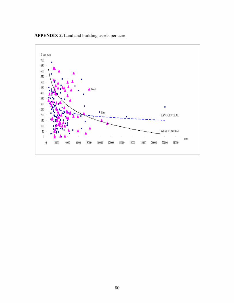
APPENDIX 2. Land and building assets per acre
EastEAST CENTRAL
West
WEST CENTRAL
050
100150200250300350400450500550600650700
0 2000 4000 6000 8000 10000 12000 14000 16000 18000 20000 22000 24000acre
$ per acre
80

APPENDIX 3. Combine costs estimation due to change in field efficiency
TCmin VC FC Ti Custom Crop acre FE
(0.80) FE
(0.75) FE
(0.80) FE
(0.75) FE
(0.80) FE
(0.75) FE
(0.80) FE
(0.75) FE
(0.80) FE
(0.75) 5000 21.89 24.7 5.18 5.52 13.22 13.21 8.13 13.87 1.86 3.186000 27.09 27.55 5.18 5.52 22.03 22.03 0 0 0 07000 24.06 24.41 5.18 5.52 18.88 18.88 0 0 0 08000 21.7 22.05 5.18 5.52 16.52 16.52 0 0 0 09000 19.87 20.21 5.18 5.52 14.68 14.68 0 0 0 0
10000 21.89 24.7 5.18 5.52 13.22 13.22 8.13 13.87 1.86 3.1811000 23.2 23.55 5.18 5.52 18.02 18.02 0 0 0 012000 21.7 22.05 5.18 5.52 16.52 16.52 0 0 0 013000 20.43 20.78 5.18 5.52 15.25 15.25 0 0 0 014000 20.36 23.01 5.18 5.52 14.16 14.15 2.38 7.74 0.55 1.7715000 21.89 24.7 5.18 5.52 13.22 17.62 8.13 0 1.86 016000 21.7 22.05 5.18 5.52 16.52 16.52 0 0 0 017000 20.73 21.08 5.18 5.52 15.55 15.55 0 0 0 018000 19.87 20.21 5.18 5.52 14.68 14.68 0 0 0 019000 20.73 22.92 5.18 5.52 13.91 17.39 3.81 0 0.87 020000 21.7 22.05 5.18 5.52 16.52 16.52 0 0 0 021000 20.91 21.26 5.18 5.52 15.73 15.73 0 0 0 022000 20.2 20.55 5.18 5.52 15.02 15.02 0 0 0 023000 20.07 22.69 5.18 5.52 13.77 14.36 4.68 6.51 1.07 1.4924000 20.96 23.67 5.18 5.52 13.22 13.21 8.13 13.87 1.86 3.18
81
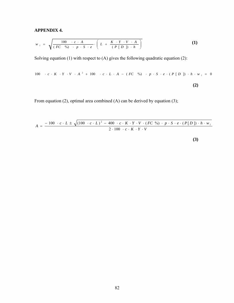
APPENDIX 4.
⎟⎟⎠
⎞⎜⎜⎝
⎛⋅⋅⋅⋅
+⋅⋅⋅⋅
⋅⋅=
hDPAVYKL
eSpFCAcw l ])[(%)(
100 (1)
Solving equation (1) with respect to (A) gives the following quadratic equation (2):
0])[(%)(100100 2 =⋅⋅⋅⋅⋅⋅−⋅⋅⋅+⋅⋅⋅⋅⋅ lwhDPeSpFCALcAVYKc
(2) From equation (2), optimal area combined (A) can be derived by equation (3);
VYKcwhDPeSpFCVYKcLcLc
A l
⋅⋅⋅⋅⋅⋅⋅⋅⋅⋅⋅⋅⋅⋅⋅⋅−⋅⋅±⋅⋅−
=1002
])[(%)(400)100(100 2
(3)
82