Embed Size (px)
Citation preview

An Analysis of a Bivariate Time Series in Which theComponents Are Sampled at Different Instants
A la recherche du temps perdus
David R. Brillinger
Abstract
It is desired to express the relationship between the components of a bivariatetime series. What is unusual is that the components are observed at different timesand that the observation times are irregularly distributed. The problem of differentsampling times is dealt with by interpolating the values of the dependent series to thetimes of the independent. This is followed by nonparametric regression to estimatethe relationship. The research is motivated by data collected at a station along theSolimoes River in central Brazil and also at a second station along a branch of theSolimoes. Of interest to geographers is the possible change in the proportion of theSolimoes waters entering the branch. This is because an increased flow of Solimoeswater into the branch might lead to the branch’s widening and becoming the mainstream. This could have substantial environmental effects.
Keywords. Amazonia; irregular sampling times; marked point process; nonpara-metric regression; river discharge; time series.
1 Introduction
Constance van Eeden has worked in many areas of statistics. Perhaps the problemthat she has studied that is closest to the work of this paper is that of densityestimation via kernels, e.g. [24]. Her work on that problem, like on many others, hasbeen via very careful analysis.
The genesis of our work is that H. O’R. Sternberg, Professor of Geography atBerkeley, visited with a problem and a data set. In statistical terms the problemconcerned the development of an instantaneous relationship between the componentsof a bivariate time series. The difficulty was that the components were sampled at

2 D. R. Brillinger
different instants. Further the spacings of the time points were irregular. The serieswere river flow rates measured at two places of a river system in Central Brazil.
According to Brazilian usage, the name Amazonas is applied to the Amazon riverbelow the mouth of the Rio Negro. Upstream from the city of Manaus the main stemis known as the Solimoes. Characteristically, the waters of the Solimoes-Amazonasdeposit, fork and come together, embracing islands approximately lenticular in shape.Strung along the river for many hundreds of kilometers, these islands split the streambed into a master channel and one or more side channels, called paranas. One suchchannel exists just upstream from the mouth of the Rio Negro, where the Solimoes(Amazon) sends off a branch, the Parana do Careiro, that rejoins the trunk streamabout 40 km. downvalley. Figure 1 shows various features. The large bright spotmidway up the figure is the city of Manaus. The light line heading across the figurefrom the left to the right is the Solimoes. The concern is the split of the Solimoesjust to the right of Manaus. The large dark river coming towards Manaus fromthe upper right is the Rio Negro. This image was taken from the NASA web siteeosweb.larc.nasa.gov.
A reason for the study is that concern has been expressed that an increased flowof Solimoes water into the branch might lead to the widening of the Careiro and evento its eventual usurpation of the trunk stream. Such a process is of scientific andsocio-economic interest, since it would destroy valuable floodplain land that supportsa significant farm population and tens of thousands of cattle. In the 1950s, the matterdrew the attention of Professor Sternberg, [19, 20]. In 1963 he coordinated a jointproject of the US Geologic Survey, the University of Brazil and the Brazilian Navy,with the objective of carrying out discharge measurements in the Brazilian Amazon,[17]. Following this initial work, the Brazilian government embarked upon a programof systematic discharge measurements in Amazonia. This supplied the data of thework. A collaborative paper planned with Professor Sternberg will highlight thegeomorphological framework of the problem, and further discuss analytical proceduresapplied to the issue, [21].
Specific questions that arise are: Does the proportion of the discharge that entersthe Careiro depend on the discharge level of the Solimoes? Is the relationship be-tween the Careiro and the Solimoes changing with time? Is the flow of the Solimoesincreasing?
Seeking answers to these questions leads to some interesting statistical problems:1. the series are sampled at different times, 2. the series are sampled irregularly,3. the relationship is possibly nonlinear and 4. the need for some theoretical prop-erties of the proposed solutions. To study the questions there appears a desire fornonparametric estimates together with estimates of the associated uncertainty andfurther an assessment of model fit. The emphasis of this paper is on the statisticalmethods rather than the geographical interpretation of the empirical results obtained.More careful checking of assumptions and serious evaluation of uncertainties is neededbefore embarking on interpretations, [21].

Sampled time series 3
Figure 1: NASA image of Central Brazil. The large bright spot towards the middle is the city ofManaus.
The sections of the paper are: Introduction, The data, Analytic formulations,Results, Goodness of fit of the models, Some extensions, and Discussion and summary.Lastly there is an Appendix laying out some analytic details and prooofs.
2 The data
The rivers’ flow rates are measured upriver on the Solimoes at a station near thetown of Manacapuru. They are also measured at a station on the Parana do Careiro.These stations are approximately 90 km. apart. Figure 1 provides a NASA image ofthe region on July 23, 2000.
The data available are for the years 1977 through 1998. Almost invariably they are

4 D. R. Brillinger
0 5000 15000 25000
0
5
10
15
20
25
30
Careiro
flow (m^3/sec)
0.5 1.0 1.5
0
5
10
15
20
velocity (m/sec)
40000 80000 140000
0
5
10
15
20
25
Solimoes
flow (m^3/sec)
0.8 1.0 1.2 1.4 1.6
0
5
10
15
20
25
velocity (m/sec)
Figure 2: Histograms of the discharge rates and velocities for the two rivers.

Sampled time series 5
•
•••
•
•
•
••••
••
••••
••
•••
•••
••••
•
•
•
•
•
•
• •
••
• • •
•
• •
•
•
••
• •
•
•
••
•
•
•
•
•
••
••
••
•
••
•
••
•
•
•
••
••
••
••
••
••
•
Flow of the Careiro (m^3/sec)
year
1980 1985 1990 1995
5000
10000
15000
20000
25000
•
••••••
•••
•••
••••••
••
•
•
••
••
•
•
••
•••
•
•
•
•
••
•
•
•
•••
•
•
••
••
•••
•
•
••
•
•
•
•
••
•••
•
• •••
•
•
•
•
• •
•
••
•
•
••
•
•
••
•
•• ••
•
•
••
Flow of the Solimoes (m^3/sec)
year
1980 1985 1990 1995
60000
80000
100000
120000
140000
160000
Figure 3: The discharges of the Careiro and the Solimoes Rivers in cubic-meters/second. Thepoints indicate the dates of available measurements.

6 D. R. Brillinger
•
•
••
•
•
•
••
•
•
•
•
•
••
•
•
•
•
••
••
•
•
••
•
•
•
•
•
•
•
• •
•
•
•• •
•
••
•
•
••
••
•
•
••
•
•
•
•
•
•
•
•
•
•
•
•
•
•
•
•
•
•
•
•
•
•
•
•
••
•
•
••
•
•
•
Flow rate of the Careiro by day of the year
day
m^3
/sec
0 100 200 300
5000
10000
15000
20000
25000
•
• •
••
•
•
••
•
••
•
•
• • •
•
•
••
•
•
• •
•
•
•
•
• •
•
••
•
•
•
•
••
•
•
•
•• •
•
•
•
•
••
•••
•
•
• •
•
•
•
•
•
•
• • •
•
•••
•
•
•
•
•
••
•
••
•
•
••
•
•
•
•
•
•
•••
•
•
•
•
Flow rate of the Solimoes by day of the year
day
0 100 200 300
50000
60000
70000
80000
90000100000
Figure 4: Observed flow rates of the two rivers plotted by day of the year.

Sampled time series 7
made on different days for the two stations because they are made by a single vesselwhich has to journey the 90km. distance between the stations. For the Solimoesthere are 100 measurements in all while for the Careiro there are 90.
The basic data are the measured river discharges, discharge being defined as: thearea of the section across the river where the measurements are made multiplied bythe water’s velocity. For these rivers the values are high going along with the factthat the Amazon outputs a substantial proportion of the world’s fresh water. Figure2 provides histograms of the flow rates and the rivers’ velocities. The rivers are seento flow at around 1 cubic-meter/sec. The discharge for the Solimoes is quite a bithigher than that of the Careiro while the velocities are comparable. The dischargeswill fluctuate with the heights of the rivers. Time series plots of the data sets areprovided in Figure 3. One notes the irregularity of the measurement dates.
Figure 4 stacks the flow data for the whole period by day of the year. An annualeffect becomes apparent with the flows being high in July-August and low at October-November. One again notes the irregularities of the measurement dates.
Figure 5 provides the cumulative counts of measurements made as a function ofdate. Such a plot is useful for examining the stationarity of the measuring process,specifically in the stationary case the points plotted will fluctuate around a straightline. One sees for example that for the Solimoes measurements were being made at ahigher rate at the beginning of the period of data collection. There are two noteablyflat stretches corresponding to measurements not being made often.
3 Analytic formulations
Let Y (t) denote the discharge rate of the Careiro at time t and X(t) that of theSolimoes. Being downriver the Careiro will be considered the dependent series andthe Solimoes the explanatory. The model that will be considered is:
Y (t) = g(X(t)) + E(t), t = 0,±1,±2, ... (1)
with the error series E having mean 0. One might ask for example is the function glinear? Is its derivative increasing? Is it changing with time?
Turning to statistical formulations of the problems one can start by thinking aboutthe classical situation where the data available are (X(t), Y (t)), t = 0, ..., T − 1, i.e.the observations of the two components are made at the same times and are equi-spaced.
For this model and smooth g(.) one could compute a kernel estimate of g(.). Withthe weight function wT (.) such an estimate has the form
g(x) =∑
t
Y (t) wT (x − X(t))/∑t
wT (x − X(t))
at the point x. If the noise series, {E(t)} is white with variance σ2 the estimate’s

8 D. R. Brillinger
Times of measurements on the Careiro
year
cum
ulat
ive
coun
t
1980 1985 1990 1995
0
20
40
60
80
Times on the Solimoes
year
cum
ulat
ive
coun
t
1980 1985 1990 1995
0
20
40
60
80
100
Figure 5: The cumulative counts of measurements made for each river.

Sampled time series 9
variance is
var{ g(x)|X} = σ2∑
t
wT (x − X(t))2/(∑
t
wT (x − X(t))2
If the variance of E(t) depends on the level of X it may be estimated for X = x by
σ2(x) =∑
t
(Y (t)− g(x))2 wT (x − X(t))/∑t
wT (x − X(t)) (2)
see Hardle [13]. This reference also provides a substantial review of nonparametricregression in the case that the noise values are independent.
Alternately to estimate the function g one might employ a local linear estimatesuch as produced by the Splus function loess(.) [11]. References concerned withnonparametric regression in the presence of time series errors include: [1], [15], [23],[14], [22] and [18].
The case of concern in this paper involves the data values
({X(σj)}, {Y (τk)}), j = 1, ..., JT ; k = 1, ..., KT
where T the observation interval is [0, T ) and where there are JT observations at thetimes {σj} for the Solimoes and KT at the times {τk} for the Careiro.
The observations are not in immediate correspondence, but many of the σj andτk are close. (See Figure 6 below which graphs the Careiro times relative to those ofthe Solimoes.) This occurrence suggests that in the particular situation at hand onemight be able to obtain useful a estimate of g.
Two approaches come to mind directly. One could interpolate the Y (τk) values toobtain estimates Y (σj) and then work with the values (X(σj), Y (σj)), j = 1, ..., JT
or one could interpolate the X(σj) to obtain estimates X(τk) and then work with thevalues (X(τk), Y (τk)), k = 1, ..., KT . The first approach appears the simpler and willbe the one pursued. The second will be discussed later and some references provided.
Consider the model (1). The interpolated values can be written:
Y (t) =∑k
Bk,1(t/T )Y (τk+1))
with the {Bk,1} B-splines of order 1, see the Appendix, [2], [12], [16] for details ofthese. Next
Y (σj) = Y (σj) + noise1
and from (1)Y (σj) = g(X(σj)) + noise2
leading toY (σj) = g(X(σj)) + noise2 + noise1 (3)
Because of the additivity of the overall error term, equation (3) has the form ofthe nonparametric regression model, with the exception that perhaps the errors are
10 D. R. Brillinger
The Careiro times relative to the Solimoe’s
lag (days)
inde
x, j
-20 -10 0 10 20
0
20
40
60
80
• •• •• •• • •••• ••• • ••
• •
•• ••
•• •
• ••••
• •••
••• • • •••• ••
•••
Figure 6: A plot of the points (j, τk − σj), j = 1, ..., J
autocorrelated and heteroscedastic. The interpolation proposed involves only the{Y (τk)} values, i.e. not the {X(σj)}. The kernel estimate of g(x) is now,
g(x) =∑j
Y (σj)wT (x − X(σj))/∑j
wT (x − X(σj)) (4)
with wT (x) = bT−1w(bT
−1x) the kernel function. However the reasonablenessof standard errors provided by naive programs is suspect their being based on anassumption of independent noise errors in (3).
In assessing the properties of the estimate it is assumed that the Careiro flow doesnot change rapidly, see Assumption b) in the Appendix. Also as it takes some timefor the waters to flow from Manacapuru to Careiro time delay δ is included in themodel writing Y (t + δ) instead of Y (t).
Some large sample properties of the estimate, e.g. the variance, are developed inthe Appendix. The estimate is asymptotically unbiased, consistent and normal.
4 Results
Already Figures 2-6 have been introduced. Figure 6 provides information on therelative timings of the Solimoes and Careiro measurements. The center vertical linecorresponds to the times of Solimoes measurements. Spread on either side of the lineare the nearby Careiro times. Careiro measurement times are seen to follow Solimoes
Sampled time series 11
•
•
••
•
•
•
••
•
•
••
•
•
•
•
•
•
•
••
••
•
•
•
•
•
•
•
•
•
•
•
••
•
•
•• •
•
• •
•
•
•
•
••
•
•
••
•
•
•
•
•
•
•
•
•
•
•
•
•
•
•
•
•
•
•
•
•
•
•
•
••
•
•
••
•
•
•
Careiro values (m^3/sec) and fitted values
. : original, __ : fit at days of measurements for the Solimoesyear
1980 1985 1990 1995
2000
3000
4000
5000
6000
700080009000
20000
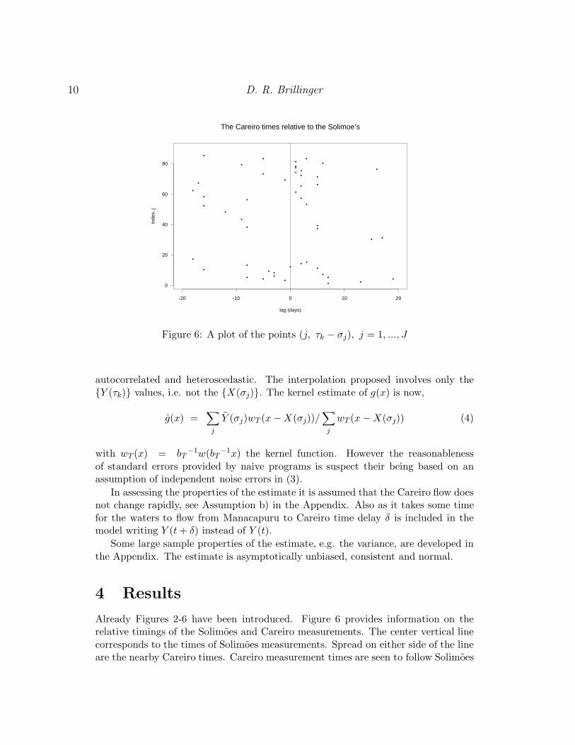
Figure 7: The points provide the positions (τk, Y (τk)), i.e. the actual data for the Careiro. Thelines join the positions (σj, Y (σj)), i.e. the interpolated values.
to an extent and many occur within 7 days. There are enough near 0 that it seemsthat reasonable estimation of g is possible. This type of rastor plot appears in [8].
We proceed following the scheme proposed in the previous section. The dataavailable are denoted {Y (τk)} for the Careiro and {X(σj)} for the Solimoes. Beingdownriver from Manacapuro the Careiro series is viewed as the dependent one.
To begin a linear interpolation spline is run through the Careiro data [2], [12].Specifically the missing Careiro discharge values were estimated by linear spline in-terpolation, i.e. a curve is passed through the points (τk, Y (τk)) and consists ofstraight lines between the points. This has the advantage that if a σj is actually aτk then the observation Y (τk) itself is used, i.e. no smoothing is carried out. Nearbytimes will have nearby values. The linear spline was employed to avoid oscillationsbetween the data points, but higher-order splines may be considered.
In the computations the logarithms of the discharges are taken as the basic valuesfor analysis since the variance of the additive noise appeared more nearly constantwhen logs were employed. Henceforth X and Y will refer to the logarithms of thebasic data. Figure 7 provides the results of the interpolation of the Y values. Theoriginal data values (τk, Y (τk)) are plotted as points. The interpolated values arejoined by lines. The fitted values do not appear inappropriate.
Next the values Y (σj + δ) are estimated where the σj are the available times forthe Solimoes and δ is an estimate of the time that it takes the water to flow betweenthe two stations. The results of the interpolation are denoted Y (σj + δ), j = 1, ..., J.
12 D. R. Brillinger
The value δ = .80 days employed is obtained using a distance of 90 km. and a speedof 1.3m/sec. (See Figure 2.)
The model considered has now become:
Y (σj + δ) = g(X(σj)) + noise (5)
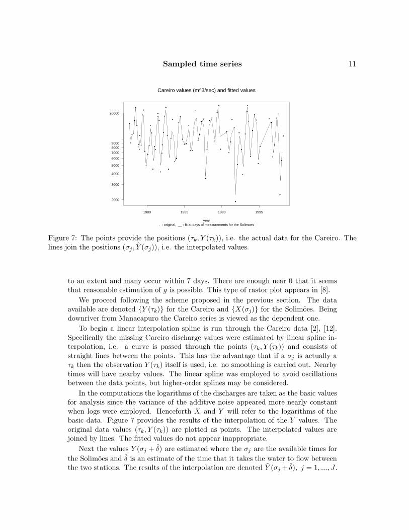
and it is to be noted that the noise is additive.Figure 8 plots the points (X(σj), Y (σj + δ)), j = 1, ..., J and as a smooth curve
the estimate of g computed via a kernel smoother using a gaussian kernel. The curveis approximately linear. The dashed lines are approximate 95% marginal confidencelimits based on the variance formula (9) of the Appendix. Some 6 or 7 of the 87points lie outside the 95% bounds.
The kernel smoother has the disadvantage of difficulties at boundaries, but it hasthe advantage of simplicity in the derivation of analytic results.
5 Goodness of fit of the model
The confidence limits of Figure 8 are basic to drawing inferences. The assumptionsof independence and constant variance involved need to be considered.
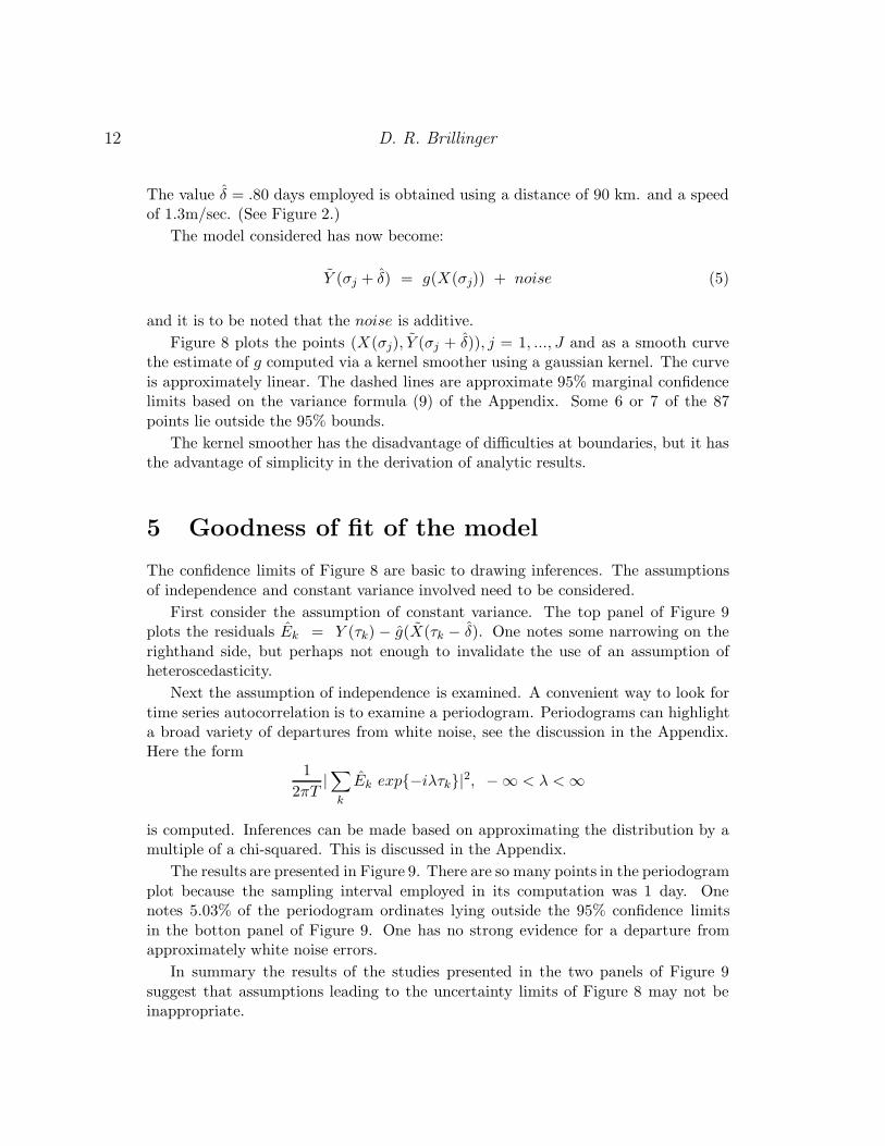
First consider the assumption of constant variance. The top panel of Figure 9plots the residuals Ek = Y (τk) − g(X(τk − δ). One notes some narrowing on therighthand side, but perhaps not enough to invalidate the use of an assumption ofheteroscedasticity.
Next the assumption of independence is examined. A convenient way to look fortime series autocorrelation is to examine a periodogram. Periodograms can highlighta broad variety of departures from white noise, see the discussion in the Appendix.Here the form
12πT
|∑k
Ek exp{−iλτk}|2, −∞ < λ < ∞
is computed. Inferences can be made based on approximating the distribution by amultiple of a chi-squared. This is discussed in the Appendix.
The results are presented in Figure 9. There are so many points in the periodogramplot because the sampling interval employed in its computation was 1 day. Onenotes 5.03% of the periodogram ordinates lying outside the 95% confidence limitsin the botton panel of Figure 9. One has no strong evidence for a departure fromapproximately white noise errors.
In summary the results of the studies presented in the two panels of Figure 9suggest that assumptions leading to the uncertainty limits of Figure 8 may not beinappropriate.

Sampled time series 13
•
•
••
••• •
••
•
•
•
•
•••
•
•
••
•
•
•
•
•
•
•
•
•
•
•
•
•
•
•
•
•
•
•
••
•
•
•
•
••
•
•
•
•
•••
•
•
• •
•
•
•
•
•
•
•
••
•
•
••
•
•
•
•
•
•
•
•
•
•
•
•
••
•
•
•
•
•••
•
•
•
•
•
•
Fitted values of the Careiro vs. the Solimoes
Flow of the Solimoes
Fitt
ed v
alue
s of
the
Car
eiro
50000 60000 70000 90000
3000
4000
5000
6000
7000
8000
900010000
20000
Figure 8: The points are (X(σj, Y (σj)), the interpolated Careiro observations plotted against theactual Solimoes values. The dashed lines are approximate marginal 95% confidence limits derivedusing expression (9).

14 D. R. Brillinger
•
•
••
•
•
•
••
•
•
••
•
•
••
••
•
••
••
•
••
•
••
•
•
•
•
••
••
•• •
•
••
•
•
••
• •
•
•
••
•
••
•
•
•
•
••
•
•
•
•
•
•
••
•
•
•
••
•
•
••
•
•
••
•
•
•
Residuals of the Careiro fit via the Solimoes
Fitted flow of the Solimoes
resi
dual
s
50000 60000 70000 90000
-0.8
-0.6
-0.4
-0.2
0.0
0.2
0.4
.
..
.
.
.
..
...
.
..
.
.
..
.
..
.
.
.
.
.
..
..
.
..
.
.
.
.
.
.
.
.
.
.
...
.
.
..
.
.
.
.
.
.
..
...
.
.
....
.
.
.
..
...
..
.
.
.
.
.
.
.
..
.
...
.
.
.
..
.
.
.
..
.
.
.
.
.
.
..
.
.
.
.
.
.
.
.
.
.
..
.
.
.
.
..
.
.
.
.
..
..
..
..
.
.
.
.
..
.
.
...
.
.
.
.
.
.
.
.
.
.
.
.
.
..
.
.
.
..
.
.
.
.
.
.
.
..
..
....
.
.
.
.
..
.
.
.
.
.
.....
.
.
.
.
.
..
.
.
.
.
.
.
.
.
.
.
.
.
..
..
.
.
.
..
.
..
.
.
.
.
.
.
.
...
.
.
..
.
.
.
....
.
.
...
.
.
.
.
.
..
..
.
.
.
.
.
.
.
.
..
..
.
.
.
..
..
.
.
.
.
.
..
.
.
.
.
.
.
.
.
.
.
.
.
.
.
.
.
.
...
.
..
.
..
.
.
.
.
.
..
.
..
.
..
.
.
.
.
.
.
.
..
.
.
...
.
.
..
.
..
..
.
.
.
.
.
.
.
..
.
.
.
.
.
.
.
.
.
.
.
.
..
.
.
.
.
.
.
..
.
..
..
..
.
.
.
.
..
.
..
.
..
.
.
.
.
.
..
.
.
.
.
.
.
.
.
.
.
.
.
.
.
.
.
.
..
.
..
.
.
.
.
...
.
.
.
.
..
.
.
.
.
.
.
.
.
.
..
.
.
..
.
.
.
.
.
.
.
.
.
.
.
...
.
.
..
.
.
.
.
.
.
.
.
.
.
.
.
.
..
.
...
.
.
...
....
.
.
..
.
.
.
.
.
.
..
..
.
.
...
.
..
.
.
..
.
.
.
.
.
.
..
.
.
.
.
.
.
.
.
.
.
.
.
.
.
.
.
.
.
.
.
..
.
.
.
.
.
.
..
.
.
.
..
.
.
.
..
.
.
.
..
.
.
..
.
..
.
.
.
.
..
.
.
.
.....
.
..
.
.
.
.
.
.
..
.
.
.
.
.
.
..
.
.
.
.
.
..
.
..
.....
.
..
.
.
.
.
.
.
.
.
...
.
.
.
.
.
.
.
.
.
.
.
.
.
.....
.
.
..
.
.
.
..
.
.
..
.
.
.
.
.
.
.
.
.....
.
.
.
.
.
.
.
.
.
.
.
.
.
..
.
.
..
.
.
.
....
.
.
.
.
...
.
.
.
.
..
..
.
....
.
.
.
.
.
.
.
.
.
.
.
.
.
..
.
.
.
...
.
.
...
.
.
.
.
.
.
....
.
.
..
.
.
.
..
..
...
.
..
..
.
.
.
.
..
.
.
.
.
.
.
..
..
.
.
.
..
.
..
...
.
..
.
.
.
.
.
.
.
.
.
.
.
..
.
.
.
.
.
.
.
.
.
...
..
..
.
.
.
.
....
.
.
.
..
.
.
.
...
.
.
.
.
.
.
.
..
.
.
.
.
.
.
.
..
.
.
....
.
.
..
.
.
.
.
.
.
.
..
..
..
..
...
.
.
.
.
.
.
.
.
.
.
.
.
.
......
.
..
.
.
.
.
.
.
....
.
.
..
.
.
.
.
.
.
.
..
.
.
.
.
..
..
..
.
.
.
.
.
.
.
.
..
.
.
.
.
.
.
.
.
..
.
.
.
.
.
.
..
..
.
.
.
.....
.
..
.
.
....
.
.
..
.
.
..
.
..
.
.
.
.
.
.
....
.
.
.
.
.
.
.
.
...
.
.
.
.
...
.
.
.
...
.
.
.
.
....
.
.
.
.
..
.
.
.
.
.
..
...
..
.
.
.
.
.
.
..
.
.
.
.
.
..
.
.
.
..
.
.
..
..
.
.
.
..
.
.
.
..
.
.
..
..
.
.
.
..
..
.
.
.
..
.
.
.
..
.
.
.
.
.
.
.
.
.
.
.
.
.
.
.
.
.
.
..
.
.
.
.
.
.
..
.
..
..
.
.
...
.
..
.
.
.
.
.
.
.
.
.
..
.
..
.
.
.
..
.
...
.
.
..
.
.
.
.
.
..
.
.
.
...
.
.
..
.
.
...
.
.
.
.
.
..
.
.
.
.
.
.
.
..
.
.
..
.
.
...
.
.
.
.
..
.
.
.
.
.
.
...
.
...
.
.
..
.
.
.
..
.
...
.
.
.
.
.
.
.
..
.
.
.
.
.
.
.
.
.
..
..
.
.
.
.
.
.
..
.
.
..
.
.
..
.
...
.
...
...
.
.
.
.
.
.
..
.
.
.
.
.
.
..
..
..
..
.
.
.
..
.
.
.
..
....
..
.
.
.
..
..
.
.
.
.
.
.
.
.
.
...
.
.
.
.
.
.
.
.
.
.
..
.
.
.
.
.
.
.
.
...
..
..
.
.
.
.
..
.
...
..
.
.
.
.
.
.
..
.
..
.
.
.
.
..
.
.
.
.
.
.
.
...
.
.
.
..
.
.
..
..
.
.
.
.
.
...
..
.
.
.
.
..
.
.
.
.
.
.
.
.
...
.
..
.
.
.
.
.
.
.
.
....
..
..
.
...
..
.
.
..
.
.
.
.
.
.
...
.
.
..
.....
.
.
.
.
..
.
...
.
.
.
..
.
.
.
..
.
.
.
.
.
.
.
...
.
.
.
.
..
.
.
.
...
.
.
.
.
.
.
.
..
.
.
.
.
..
.
.
.
...
..
.
.
..
.
.
.
.
.
.
.
.
..
.
.
.
.
.
.
.
.
..
..
.
..
.
.
.
.
.
.
...
.
.
.
.
..
..
.
.
.
.
.
..
.
.
...
.
.
.
..
.
.
....
.
.
..
.
....
.
.
.
..
.
.
..
..
.
...
.
....
..
..
.
.
.
.
.
.
.
.
..
.
.
.
.
.
.
.
.
.
.
.
.
..
.
.
.
..
.
..
.
.
..
..
.
.
..
.
.
.
..
.
.
.
.
.
.
.
.
..
.
.
.
.
.
.
.
..
.
.
.
.
..
..
.
....
.
.
.
.
.
.
.
.
.
..
...
.
.
.
..
.
.
.
.
...
.
.
.
..
.
.
.
.
.
..
.
.
.
.
.
.
...
.
.
..
.
.
.
.
...
.
..
.
.
.
.
.
.
.
..
.
..
.
.
.
.
..
...
..
...
.
.
.
.
.
.
.
.
.
.
..
.
.
.
.
.
.
..
.
.
..
.
.
.
.
..
.
.
..
..
.
..
.
.
.
.
.
.
.
.
..
.
..
.
.
..
.
.
...
.
.
.
.
..
.
...
.
.
..
.
....
..
.
.
...
..
.
.
.
.
.
.
.
..
.
.
...
.
..
.
.
.
.
.
.
.
.
.
..
.
.
..
.
.
.
.
.
..
.
.
.
..
.
.
.
.
.
.
.
.
.
.
..
.
.
.
.
..
.
..
.
.
.
.
.
..
.
.
.
.
.
.
.
.
.
..
.
.
..
.
.
.
.
.
.
.
..
.
.
.
.
.
..
...
.
.
..
.
.
.
.
..
.
..
.
.
.
.
.
.
.
.
..
.
.
.
.
...
..
.
.
.
.
...
..
.
.
.
.
.
.
.
.
.
.
.
.
..
.
.
.
...
.
.
.
.....
..
.
.
.
.
.
...
...
.
.
.
.
.
..
.
.....
.
.
.
.
.
.
.
.
.
.
.
..
.
.
.
...
.
.
.
.
.
.
.
.
.
.
.
.
.
..
.
..
.
.
.
.
.
.
.
.
.
.
.
.
.
.
.
...
.
.
.
.
.
.
.
.
.
.
.
.
.
..
.
.
.
.
.
..
..
.
.
.
.
.
.
.
.
..
..
.
.
.
.
.
..
.
.
.
.
.
.
..
.
.
.
..
.
.
.
.
.
.
.
.
.
.
.
.
...
.
.
..
.
..
..
.
..
.
..
.
.
.
.
.
.
.
.
.
.
.
.
.
.
.
...
.
.
.
.
.
.
.
.
.
.
.
.
.
.
..
.
..
.
.
.
.
..
.
..
.
.
.
.
..
.
.
.
.
.
.
.
..
.
.
..
.
....
...
..
.
.
.
.
.
...
.
.
.
.
.
...
.
.
.
.
.
.
..
......
.
.
.
.
.
..
..
.
.
.
.
.
.
.
.
.
.
.
.
.
.
..
.
..
.
.
.
.
.
.
.
.
.
..
.
..
.
.
..
.
.
.
..
.
.
..
.
..
.
.
.
...
.
.
.
.
..
.
.
.
.
.
...
...
....
.
.
.
.
.
.
..
.
.
.
.
.
.
...
.
.
.
..
.
...
.
.
.
..
.
..
.
...
.
.
.
.
.
.
.
.
.
..
.
.
.
.
.
.
.
.
.
.
..
.
.
.
.
...
.
.
.
.
.
.
..
.
.
.
...
..
.
.
.
.
.
.
.
.
.
...
..
.
..
..
.
..
.
.
.
.
.
.
.
...
.
.
.
.
.
.
..
.
.
....
.
.
.
.
.
.
...
..
.
.
.
...
.
..
.
.
.
.
.
.
..
.
.
.
.
.
.
.
.
..
...
.
..
..
.
.
.
.
.
.
.
.
..
.
...
.
...
..
.
.
.
.
..
....
.
.
.
.
.
...
.
.
...
.
.
.
..
.
...
.
.
.
.
.
.
..
...
.
.
.
...
....
.
.
.
.
.
.
....
.
.
.
.
..
.
.
.
.
.
.
.
.
.
.
..
....
.
.
..
.
.
.
.
.
.
.
..
.
...
.
.
..
.
.
.
.
..
..
.
.
.
.
.
.
.
.
.
.
..
...
...
.
.
.
.
.
.
..
.
.
.
.
...
.
.
.
..
.
.
.
.
.
.....
.
..
.
...
.
.
.
.
.
..
.
.
....
...
.
..
..
.
.
.
.
.
.
.
.
.
.
..
.
.
.
..
.
...
.
.
.
.
..
..
.
.
.
.
..
.
.
..
.
.
.
.
.
.
.
.
.
.
.
.
.
.
.
.
.
.
.
.
...
.
.
.
.
.
.
.
.
.
..
.
.
.
.
.
.
.
.
.
.
.
.
.
.
.
.
.
.....
.
.
.
.
.
.
.
.
.
.
..
.
..
..
..
.
.
..
.
.
.
.
.
.
.
..
.
.
.
.
.
...
.
.
.
..
...
.
.
.
.
..
.
.
..
.
.
..
.
.
..
.
..
..
.
.
.
..
.
..
.
.
.
..
.
..
.
...
.
.
...
..
.
..
.
.
.
.
.
.
...
.
.
....
.
.
.
.
.
.
.
..
.
....
.
.
.
.
.
.
.
.
.
..
.
.
...
.
.
.....
.
.
.
.
..
..
..
.
.
.
.
.
.
.
.
..
.
.
.
...
.
.
.
..
.
..
.
..
.
.
.
.
.
.
...
.
.
.....
.
..
.
.
.
.
..
..
..
..
.
.
.
.
.
.
.
.
.
.
.
.
...
.
.
.
..
.
.
....
.
.
.
.
..
.
.
..
.
.
.
..
.
.
....
..
.
.
.
.
..
.
.
.
.
.
.
.
.
...
.
.
.
..
.
...
.
.
.
.
..
.
.
.
.
.
..
.
.
...
.
.
.
.
..
..
..
..
..
.
.
..
.
.
.
.
..
.
.
.
.
.
.
..
.
.
...
.
.
..
.
.
.
.
..
.
..
..
.
..
.
....
.
.
.
.
..
.
.
.
.
..
.
.
.
...
.
.
.
.
.
.
..
.
.
..
.
.
......
.
.
..
.
.
.
.
.
..
.
..
.
..
.
.
.
...
.
.
.
.
.
.
.
.
.
..
.
.
.
..
.
.
.
.
.
.
.
..
.
.
.
..
...
..
.
..
.
.....
.
.
..
.
.
.
.
.
..
.
.
.
.
.
..
.
.
.
..
.
.
..
.
.
.
.
.
.
..
.
..
..
.
.
.
.
.
.
...
.
....
.
.
..
.
.
.
.
.
.
.
.
.
.
.
.
.
.
..
.
.
.
.
.
.
.
.
.
.
.
.
..
.
.
.
.
.
..
...
.
.
.
.
..
.
.
.
.
....
.
.
.
.
.
.
.
.
.
.
.
.
.
..
.
.
.
..
.
.
.
...
.
...
.
.
.
.
.
.
.
.
.
.
.
.
.
....
.
.
.
..
.
.
.
.
..
.
...
.
.
.
.
.
.
.
.
.
.
.
.
.
.
.....
.
..
.
.
.
.
..
.
..
.
.
.
..
.
.
..
..
.
..
..
.
...
.
.
.
.
.
.
.
.
.
.
.
.
.
.
.
.
.
..
.
.
.
.
.
.
.
.
.
.
.
.
..
.
.
.
..
.
.
.
..
.
..
.
.
..
.
.
..
.
..
.
..
..
.
.
.
.
.
.
..
.
.
...
..
.
.
.
..
.
..
...
..
.
.
.
.
.
Periodogram of the residuals
95% limitsfrequency (cycles/day)
0.0 0.1 0.2 0.3 0.4 0.5
0.0001
0.0010
0.0100
0.1000
1.0000
10.0000
Figure 9: The top panel provides the residuals of the Careiro data as explained by the interpolatedSolimoes values. The bottom panel provides the periodogram. The horizontal line in it is theaverage of all the periodogram values. The dashed lines in the lower panel provide approximate95% marginal confidence limits.

Sampled time series 15
6 Discussion and summary
The series {X(t}) and {Y (t)} were sampled irregularly and at different times, yet ithas proved possible to proceed to study their relationship via smoothing and Fourieranalysis. To begin some descriptive statistics were presented, then modelling wascarried out. An approximate linear dependence of the Careiro flow upon that of theSolimoes flow was found.
Contributions of the work include assessing the whiteness of a sampled time seriesvia a periodogram and derivation of some properties of a nonparametric estimateinvolving interpolation of the dependent variate’s values.
The method of predicting the Y (σj) could perhaps be improved, e.g. by includinga seasonal effect explanatory series. There are other methods of constructing approx-imate confidence intervals such as the bootstrap. Also the problem of the estimationof the smoothing parameter, bT , might be considered.
As mentioned earlier an alternate approach to dealing with the irregularity ofobservation times is to interpolate the {X(σj}) to the {τk} time points. This may beimplimented by an interpolation spline as was done to obtain the {Y (σj)}. Supposingthe values (X(τk), Y (τk)) are then employed in a nonparametric regression analysisthe circumstance could be viewed as an errors in variables problem. One differencefrom the classical situation though is that here one has some control over the bias andthe error variance through choice of the interpolation/smoothing procedure. Thereis a literature on this situation, [3] and [10]. There is also a related literature onendogeneity in nonparametric models [5]. The approach actually implimented is sim-pler because of the additivity of the noise, the fact that one may argue conditionallyon the X-values and because it seemed allowable to treat the error values as whitenoise. It remains to be seen which approach leads to better estimates and this surelydepends on the values of JT and KT , which series can be better interpolated amongstother things. It may be that interpolating each series to the same equi-spaced grid isto be preferred.
In connection with the interpretation of the results of the data analyses it needsto be remembered that the work is preliminary. It will be further developed in [21].
Acknowledgements
The work of this paper was supported by NSF Grants DMS 97-04739, DMS 99-71309 and DMS 02-03921. As indicated at the outset, the problem and the datawere brought to this writer’s attention by Professor H. O’R. Sternberg of the De-partment of Geography, University of California, Berkeley. I thank him profusely forthe interactions on this topic and on so many others. Professor Sternberg obtainedthe data from: CPRM (Companhia de Pesquisas de Recursos Minerais), ANEEL(Agencia Nacional de Energia Eletrica), DNAEE (Dep. Nacional de Aguas e EnergiaElectrica) through the courtesy of Eduardo de Freitas Madeira and Fernando Pereira

16 D. R. Brillinger
de Carvalho.Jim Powell made some helpful comments and provided a preprint of [5]. Phil
Spector helped with some Splus coding. The Referees made comments leading toimprovements in the paper. One suggested the consideration of the log transform.Michael Last carried out a literature search on nonlinear models involving measure-ment errors. I thank them all.
Constance van Eeden has done a great deal for statistics in Canada. It is indeedan honour to know her and to contribute to her Festschrift. (I hope that she won’tbe put off by my not so “very careful analysis”.)
David R. Brillinger, Department of Statistics, University of California, Berkeley, CA94720-3860, [email protected].
References
[1] N. S. Altman. Kernel smoothing of data with correlated errors. J. Amer. Statist.Assoc., 85:749–759, 1990.
[2] K. E. Atkinson. An Introduction to Numerical Analysis. J. Wiley, New York,1978.
[3] S. M. Berry, R. J. Carroll, and D. Ruppert. Bayesian smoothing and regressionsplines for measurement error problems. J. Amer. Statist. Assoc., 97:160–169,2002.
[4] P. Bloomfield. Spectral analysis with randomly missing observations. J. RoyalStatist. Soc., 32:369–380, 1970.
[5] R. Blundell and J. L. Powell. Endogeneity in nonparametric and semipara-metric regression models. In L.Hansen and S. Turnovsky, editors, Advances inEconomics and Econometrics: Theory and Applications, Eighth World Congress,Econometric Society Monograph Series. Cambridge University Press, 2002.
[6] D. R. Brillinger. Time Series: Data Analysis and Theory. Holt-Rinehart, NewYork, 1975.
[7] D. R. Brillinger. A continuous form of post-stratification. Ann. Inst. Stat. Math.,31:271–277, 1979.
[8] D. R. Brillinger. Nerve cell spike train data analysis: A progression of technique.J. Amer. Statist. Assoc., 87:260–272, 1992.
[9] D. R. Brillinger. Examining an irregularly sampled time series for whiteness.Resenhas, 4:423–431, 2000.
[10] R. J. Carroll, D. Ruppert, and L. A. Stefanski. Measurement Error in NonlinearModels. Chapman and Hall, London, 1995.

Sampled time series 17
[11] W. S. Cleveland, E. Grosse, and W. M. Shyu. Local regression models. In J. M.Chambers and T. J. Hastie, editors, Statistical Models in S, pages 309–376,Pacific Grove, California, 1992. Wadsworth.
[12] C. de Boor. A Practical Guide to Splines. Springer, New York, 1978.
[13] W. Hardle. Smoothing: With Implementation in S. Springer, New York, 1991.
[14] W. Hardle and P-D. Tuan. Some theory on M-smoothing of time series. J. TimeSeries Analysis, 7:191–204, 1986.
[15] J. D. Hart. Kernel regression estimation with time series errors. J. Royal Statist.Soc., 53:173–187, 1991.
[16] T. J. Hastie and R. J. Tibshirani. Generalized Additive Models. Chapman andHall, London, 1990.
[17] R. E. Oltman, H. O’R. Sternberg, Ames F. C., and L.C. Davis, Jr. AmazonRiver Investigations, Reconnaissance Measurements of July 1963, volume 486 ofGeological Survey Circular. U.S. Department of the Interior, Washington, 1964.
[18] P. M. Robinson. Large-sample inference for nonparametric regression with de-pendent errors. Technical Report EM/97/336, London School of Economics,London, 1997.
[19] H. O’R. Sternberg. Radiocarbon dating as applied to a problem of Amazonianmorphology. In Comptes Rendus XVIIIe Congres International de Geographie,Rio de Janeiro - 1956, volume 2, pages 399–424, Rio de Janeiro, 1960. ComiteNational du Bresil.
[20] H. O’R. Sternberg. A agua e o Homem na Varzea do Careiro (2nd ed.), volume1, 2 of Colecao Friedrich Katzer. CNPq Museu Paraense Emilio Goeldi, Belem,Para, 1998.
[21] H. O’R. Sternberg and D. R. Brillinger. Streamflow at branching channels;geomorphic and statistical issues from a case study in the Brazilian Amazon. Inpreparation, 2002.
[22] L. Tran, G. Roussas, S. Yakowitz, and B. T. Van. Fixed-design regression forlinear time series. Ann. Statist., 24:975–991, 1996.
[23] Y. K. Truong. Nonparametric curve estimation with time series errors. J. Stat.Planning Inference, 28:167–183, 1991.
[24] C. van Eeden. Mean integrated squared error of kernel estimators when thedensity and its derivative are not necessarily continuous. Ann. Inst. Stat. Math.,37:461–472, 1985.
Appendix
Throughout the Appendix the arguments are conditional on X as is usual in statisticalinference.

18 D. R. Brillinger
The theorems do not present best possible results rather the material has beenset up to suggest possible routes for later work. In the data analyses linear splineshave been employed, and the analytic results developed. Further the error processE has been assumed to have cumulants of all orders in order to obtain asymptoticnormaility directly. Lastly the case of a kernel smoother is the one studied. Thiswas done in the interests of simpler proofs. The results are preliminary, proofs aresketched and assumptions have been set down rather casually. It is possible to boundthe errors of all the approximations however.
Consistency and asymptotic normality.The model considered is
Y (t) = g(X(t)) + E(t), t = 0, ..., T − 1
with the distinction that the data values available are
X(σj), j = 1, ..., JT ; Y (τk)), k = 1, ..., KT
with 0 ≤ σk, τk < T . The results are developed for the case of a kernel smoother.Notations.
The spline of order 1 based on the points {(τk, Y (τk))} is denoted Y (t). It maybe written
Y (t) =∑k
Y (τk+1)Bk,1(t/T )
where the k-th B-spline function of degree 0 with knots τk is given by
Bk,1(t/T ) = (t − τk)/(τk+1 − τk) for τk ≤ t < τk+1
= (τk+2 − t)/(τk+2 − τk+1) for τk+1 ≤ t < τk+2
and equals 0 otherwise.The kernel smooth studied to estimate g(x0) is
g(x0) =∑j
wT (x0 − X(σj))Y (σj) /∑j
wT (x0 − X(σj)) (6)
In this definitionwT (x) = b−1
T w(b−1T x)
with bT > 0 a binwidth.To develop asymptotic approximations the following forms are used
g(X(t)) = HT (t) = h(t/T ), X(t) = x(t/T )
For a a function on [0,1]||a|| = sup
u|a(u)|
Sampled time series 19
Assumptions. Basic ones includea) The kernel w is non-negative, of finite support, continuous and
∫w(u)du = 1.
b) The functions h and x are in C1[0, 1]. The equation x(u) = x0 has a finitenumber of solutions.
c) The sequence {τk} is strictly increasing. There exist FM (u) and 1-1 FN (v) suchthat
FM(u) =1JT
#{σj/T ≤ u; j = 1, ..., JT} → FM (u)
andFN (v) =
1KT
#{τk/T ≤ v; k = 1, ..., KT} → FN (v)
weakly as T → ∞. The functions FM and FN have densities fM and fN .d) The process E is zero mean white noise and has cumulants of all orders.
Results.Lemma 1. Under Assumption b)
HT (t) = HT (t) + O(∆2TT−2||h(2)||) (7)
as T → ∞ where ∆T = max{τk+1 − τk, k = 1, ..., KT} and h′ is the derivative ofh. The error term is uniform in t.Proof. Since h is in C1[0, 1], h the spline of order 1 passing through the points(vk, hk = h(vk)), satisfies
|h(v) − h(v)| ≤ 18∆2 sup
v|h(2)(v)|
where ∆ = max{vk+1 − vk}, [12]. The result of the Lemma follows taking v = t/T ,vk = τk/T and HT (t) = h(t/T ).Theorem 1. Under the Assumptions
E{g(x)} = g(x) + O(bT ) + O(∆2TT−2) (8)
Proof. To begin because the spline is linear in the data values
Y (t) = HT (t) + E(t)
From the result (7) and the fact that the series E has mean 0
E{∑j
Y (σj)wT (x − X(σj))} /∑j
wT (x − X(σj))
=∑j
(g(X(σj)) + O(∆TT−1))wT (x − X(σj)) /∑j
wT (x − X(σj))
From the non-negativity, the finite support of w and the boundedness of the derivativeof h
g(X(σj)) = g(x) + O(bT )

20 D. R. Brillinger
uniformly giving the result.Corollary. Under the Assumptions and if ∆T /T, bT → 0 as T → ∞ the estimateg(x) is asymptotically unbiased.Theorem 2. Under the Assumptions with the E(τk) independent and of variance σ2
var{g(x0)} = σ2∑k
[∑j
wT (x0 − X(σj))Bk,1(σj
T)]2 / (
∑j
wT (x0 − X(σj)))2 (9)
Proof. By construction
E(t) =∑k
E(τk+1)Bk,1(t
T)
Now∑j
E(σj)wT (x − X(σj)) =∑k
[∑j
Bk,1(σj
T)wT (x − X(σj)]E(τk+1) (10)
and the result is immediate since the error series, E, is white noise with variance σ2.The form (9) may be contrasted with that were the values X(σj), Y (σj)), j =
1, ..., JT available. The variance then would be
σ2∑j
wT (x0 − X(σj))2 / (∑j
wT (x0 − X(σj)))2
Corollary. With E(τk) = Y (τk)− g(X(τk)) the error variance σ2 may be estimatedby ∑
k
E(τk)2 / KT
The asymptotic behavior of the variance may be investigated further. In theproofs below certain sums will be replaced by integrals. The accuracy of theseapproximations may be bounded using Lemma 4 below. Basically one will wantsupu|#{σj/T ≤ u}/JT − FM (u)| and supv |#{τk/T ≤ v}/KT − FN (v)| to becomesmall at a fast enough rate as JT , KT → ∞.
Consider the variance at X(t) = x0.Lemma 2. Under asumptions like those already indicated plus bT → 0 and JT → ∞as T → ∞ the denominator of (6) is asymptotically
(JT
∑′fM(x−1(x0))/|x′(x−1(x0))|)2
where the sum,∑′ is over the solutions of x(u) = x0.
Proof. Consider1JT
∑j
wT (x0 − x(σj/T ))

Sampled time series 21
=∫
wT (x0 − x(u))dFM(u)
≈∫
b−1T w(b−1
T (x0 − x(u))fM(u)du
≈∑′
fM (x−1(x0)1
|x′(x−1(x0))|∫
w(u)du
Bounds on the error of approximating the sum by an integral may be found usingLemma 7.Lemma 3. Under the assumptions of Lemma 2 plus KT → ∞ the numerator of (6)is asymptotically
J2T
1bTKT
∑′fN (x−1(x0)
−1fM (x−1(x0))2
1|x′(x−1(x0)|
∫w(u)2du
Proof. Consider
∑k
[∑j
Bk,1(σj
T)wT (x0 − X(σj))]2 ≈ J2
T
∑k
[∫
Bk,1(u)wT (x0 − x(u))fM(u)du]2
Because 2TBk,1(u)/(τk+2−τk) acts like a Dirac delta function centered at τk+1/T fora continuous function a
∫Bk,1(u)a(u)du ≈ a(τk+1/T )(τk+2 − τk)/2T
With the approximation
τk+2 − τk
2T≈ 1
KTfN (τk/KT )
the expression being studied is approximately
J2T
KT
∑k
(τk+2 − τk)2
4T 2wT (x0−x(τk+1/T ))2fM(τk+1/T )2 ≈ J2
T
KT
∫ 1fM (v)2
wT (x0−x(v))2fM(v)2fN (v)dv
With the change of variable s = x(v) this becomes
J2T
KT
∫wT (x0 − s)2fM (x−1(s))2fN (x−1(s))−1 1
|x′(x−1(s))|ds
giving the indicated result as T → ∞.Corollary 1. The variance of g(x0) is asymptotically
σ2
bTKT
∑′fN (x−1(x0))−1fM (x−1(x0))2
1|x′(x−1(x0)|
∫w(u)2du / (
∑′fM (x−1(x0))/|x′(x−1(x0))|)2
Corollary 2. Assuming in addition that bTKT → ∞ the estimate is consistent.

22 D. R. Brillinger
The result simplifies when fN ≡ fM .Theorem 3. Assuming that E(t) has finite cumulants, κm, m = 1, 2, ...
(g(x) − E{g(x)}) /√
var{g(x)}
is asymptotically normal with mean 0 and variance 1.Proof. The cumulant of order m of (10) is
κm
∑k
[∑j
Bk,1(σj
T)wT (x0 − X(σj))]m
Arguing as above one sees that this is asymptotically
κm
bm−1T Km−1
T
∑′fN (x−1(x0))1−mfM (x−1(x0))m 1
|x′(x−1(x0)))|∫
w(u)mdu
The standardized cumulants of order m > 2 are seen to tend to 0 as T → ∞. Thenormal distribution being determined by its moments, the Theorem follows.
Sampled time series.Consideration next turns to the logic lying behind the model assessment via the
periodogram of the residuals.A sampled time series may be represented as {R(t) = M(t)X(t), t = 0,±1,±2, ...}
where {X(t), t = 0,±1,±2, ...} is the series and {M(t), t = 0,±1,±2, ...} is a 0-1valued series representing the sampling times, {σj}. M takes on the value 1 whenthe X observation is present and 0 otherwise. The non-zero values of R are the{X(σj)}. The series R reflects the statistical properties of the series X and M . Forexample if X and M are mutually independent and stationary with power spectrafXX(λ), fMM(λ) then the process R has power spectrum
fRR(λ) = c2MfXX(λ) +
∫ π
−πfMM(λ − α)fXX(α)dα
assuming further that X has mean 0 and that M has mean cM . This expression wasgiven in [4] and follows from Example 2.10.4 in [6]. From it one sees that if X is whitenoise then the spectrum of R is constant. The heuristics of this result are clear: ifthe series is white then the sampled values are a separate selection and themselveswhite. One has a means of assessing whether a sampled time series is white. (Theseremarks correct some incorrect discussion in [9].)
The spectrum of the series R may be estimated by smoothing the periodogram
12πT
|T−1∑
0
e−iλtR(t)|2 =1
2πT|KT∑1
e−iλτkX(τk)|2

Sampled time series 23
for example. In many situations when LT periodogram ordinates are averaged fRR(λ)/fRR(λ)is distributed approximately as χ2
2LT/2LT . When LT → ∞ as T → ∞ the asymp-
totic distribution of log(fRR(λ)/fRR(λ)) is normal with mean 0 and variance 1/LT .For examples of the assumptions leading to such results see e.g. [6]. Such results
are often used to set confidence limits for a spectrum estimate. They may also beused to test whether fRR(λ) = γ2, e.g. by constructing confidence bounds in a plotof the estimated spectrum fRR(λ). Such a test will be consistent at frequency λ asLT → ∞ for √
LT log(fRR(λ)/γ2) =√LT log(fRR(λ)/fRR(λ) +
√LT log(fRR(λ)/γ2)
The first term here is asymptotically standard normal while when fRR(λ) 6= γ2 theabsolute value of the second grows to infinity as LT → ∞.
Figure 9 presents the spectral results taking R = Ek = Yk − gk. In Figure 9 thebaseline plotted is an estimate of γ2, specifically the average of all the periodogramordinates. It tends to
∫fRR(λ)dλ and has variance O(1/T ), i.e. its variability may
be neglected.Lemma 4. Let h(u) be a function with variation V (h). Let F (u) be a distributionfunction on (−∞,∞). Given u1, u2, ..., uJ let
F (u) = #{j|uj ≤ u}/J
and letdJ = sup
u|F (u)− F (u)|
Then| 1J
∑j
h(uj) −∫
h(u)du| ≤ V (h)dJ
Proof. See [7].