Decision maps for bivariate time series with

potential threshold cointegration

Robert M. Kunst

University of Vienna,

Department of Economics,

BWZ, Bruenner Strasse 72,

A�1210 Wien (Vienna), Austria

Abstract

Bivariate time series data often show strong relationships between the two com-

ponents, while both individual variables can be approximated by random walks

in the short run and are obviously bounded in the long run. Three model

classes are considered for a time-series model selection problem: stable vector

autoregressions, cointegrated models, and globally stable threshold models. It

is demonstrated how simulated decision maps help in classifying observed time

series. The maps process the joint evidence of two test statistics: a canonical

root and an LR�type speciÞcation statistic for threshold effects.

Keywords: Bayes test, model selection, nonlinear time series, cointegration,

simulation.

1 Introduction

Bivariate time series data often exhibit features such as the pair of retail interest

rates in Figure 1. The two component series appear to be closely linked such

that deviations from each other are relatively small. For long time spans, the

variables move up or down the positive diagonal, with very little memory with

respect to this motion. Individually, the series appear to be well described as

random walks or at least as Þrst-order integrated processes with low autocorre-

lation in the differences. Eventually, however, the upward or downward motion

appears to hit upon some outer boundary and is reversed, such that all obser-

vations are contained in a bounded interval, with unknown bounds. A good

example for such pairs of time series data are interest rates, such as saving and

loan rates or bill and bond rates, though a deep economic analysis of interest

rates is outside the scope of this paper. It can be observed that they attain their

maximum in phases of high inßation and that their minimum is usually strictly

positive. Similar pairs of time series may appear in non-economic data, such

as water ßow data from two rivers (see Tsay, 1998). Such series are charac-

terized by three features: individual behavior close to but not exactly equal to

random walks for considerable time spans; parallel movement in both variables,

though no exact relation and possibly slight deviations of the �equilibrium� from

the positive diagonal; in the long run, �mean reversion� determined by unknown

upper and lower bounds.

This paper is concerned with selecting an appropriate time series model for

such data, if the set of available classes is given by the three following ideas.

Firstly, the observed reversion to some distributional center may suggest a lin-

ear stable vector autoregression. This model class has the drawback that the

autoregression is unable to reßect the random movement in the short run. Sec-

ondly, this movement and the obvious link between the components may suggest

a cointegrated vector autoregression. Particularly for interest rates of different

maturity, this idea has been popular in the econometric literature, see for ex-

ample Campbell and Shiller (1987), Hall et al. (1992), or Johansen and

1

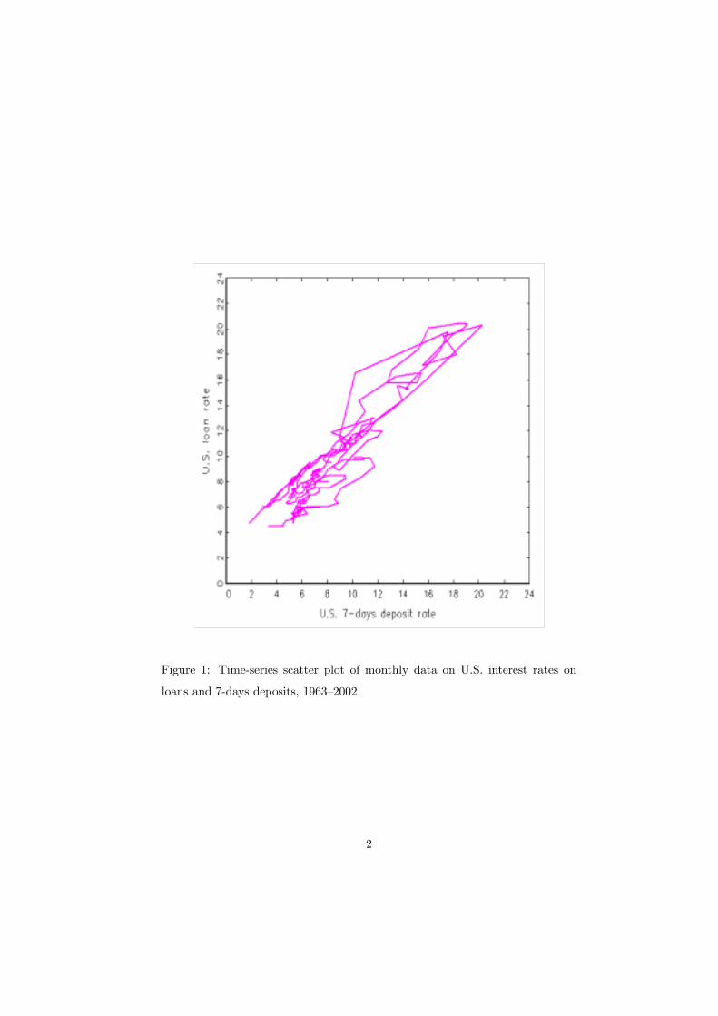
Figure 1: Time-series scatter plot of monthly data on U.S. interest rates on

loans and 7-days deposits, 1963�2002.

2

Juselius (1992). Enders and Siklos (2001) state that �it is generally agreed

that interest-rate series are I(1) variables that should be cointegrated�. The

drawback of this model class is that it does not match the long-run bounded-

ness condition. The model contains a unit root, is non-ergodic and inappropri-

ate from a longer-run perspective (seeWeidmann, 1999, for a similar argument

in economics). Thirdly, one may consider a mixture of the two models, with

cointegration prevailing in a �normal� regime and global mean reversion in an

�outer� regime. This idea yields a threshold cointegration speciÞcation, as used

by Jumah and Kunst (2002), for interest rates on loans and deposits. The

drawback of the model is that it is nonlinear and contains some poorly identiÞed

parameters.

The concept of threshold cointegration was developed by Balke and Fomby

(1997, henceforth BF) who assumed a version with cointegration in the outer

regime and an integrated process without cointegration in an inner regime (a

�band�). Jumah and Kunst (2002) suggested a modiÞcation of BF�s model

that is in focus here. Threshold cointegration models were also considered by

Enders and Granger (1998), Enders and Falk (1998), and Enders and

Siklos (2001). These contributions focus on asymmetric adjustment to dise-

quilibrium and hence they mainly use two-regime or single-threshold models.

Hansen and Seo (2002) analyze hypothesis testing for single-threshold cointe-

gration models and assume cointegration in both regimes, though with different

cointegrating vectors. Like BF, Lo and Zivot (2001) consider the case of three

regimes, with cointegration in the lower and upper regimes and no cointegration

in the central regime. While these authors allow for asymmetric reaction or dif-

ferent cointegrating structures across regimes, only symmetric reaction outside

the band will be considered here, due to the limited information that is pro-

vided by the few observations in the outer region of our models. Weidmann

(1999) analyzed bivariate time series of an inßation index and an interest rate

and suggested a three-regimes model that is close to the one used here. While

his model assumes different cointegration structures across regimes and achieves

global stability by the choice of cointegrating vectors in the outer regimes, we

3

impose local stability in the outer regimes. Tsay (1998) considered related

models in a more general framework. Caner and Hansen (2001) investigate

univariate threshold integrated models and focus on the asymptotic distribu-

tions of test statistics.

Threshold cointegration models are particular threshold vector autoregres-

sions of the SETAR (self-exciting threshold autoregression) type that was con-

sidered by Chan et al. (1985), Tong (1990), Chan (1993), and Chan and

Tsay (1998). Particularly Chan et al. (1985) found that stability in the outer

regimes is sufficient, though not necessary, for global stability and geometric

ergodicity. It follows that the models suggested here are globally stable and

geometrically ergodic. A proof of this important property has been added to

this paper as an appendix.

The decision set consists of three elements: the stable vector autoregression,

the linear cointegration model, and the threshold cointegration model. Each

model class deserves attention as a possible data-generating mechanism. It is

therefore interesting to study methods that allow a selection among the classes

on the basis of observed data. Candidates for discriminatory statistics are like-

lihood ratios for any two model classes or approximations thereof. The theory

of likelihood ratios for the Þrst and the second class has been developed by

Johansen (1988), hence it is convenient to include this ratio in the vector sta-

tistic. As another statistic, we add an approximation to the likelihood ratio of

the Þrst and the third class.

Model selection is a Þnite-action problem. It is obvious that a mere applica-

tion of the standard binary Neyman-Pearson framework of null and alternative

hypotheses severely restricts the set of decision procedures. A joint evaluation of

test statistics allows a much richer set than consideration of test sequences only.

Here, the three competing model classes are modeled as three alternative Bayes

data measures. Each measure can be conditioned on the values of a vector sta-

tistic, such that the probability for each hypothesis can be evaluated conditional

on the given or observed test statistic. The model or hypothesis with maximum

probability is then the suggested choice for the observed value of the statistic. In

4

the space of null fractiles of the test statistics, one obtains �decision maps� that

show distinct regions of preference for each model class. This approach builds

on a suggestion by Hatanaka (1996) and was used by Kunst and Reutter

(2002), among others. For the present problem, non-informative prior distrib-

utions are elicited on the basis of Jordan distributions (see also Kunst, 2001).

Discrete uniform priors over the three hypotheses are allotted implicitly. All

calculations of decision maps have been conducted by means of simulation. De-

cision maps are particularly well suited for model selection based on the joint

evaluation of two test statistics. Conditional on the priors for the rival hypothe-

ses, the decision according to the map is optimal in the sense that any deviation

from the suggested selection increases the probability of incorrect classiÞcation.

The remainder of this paper is structured as follows. Section 2 explains the

decision maps approach and details the properties of the entertained models,

including the elicitation of non-informative prior distributions. Section 3 reports

the simulation results, including the maps and their tentative interpretation.

Section 4 concludes.

2 Designing the simulation

2.1 Decision maps

The decision maps approach can be applied to all parameterized problems

(fθ, θ ∈ Θ) for Þnite-dimensional Θ, where a decision is searched among a Þ-nite number of rival hypotheses (a partition of Θ), preferably on the basis of a

bivariate vector statistic. For a univariate statistic, the maps collapse to inter-

vals on the real line. For vector statistics with a higher dimension, the visual

representation of the maps meets technical difficulties.

Assume a decision concerns the indexed set of hypotheses {Hj = {θ ∈ Θj},j = 1, . . . , h}. Usually, model selection utilizes h− 1 likelihood-ratio statisticsS1(j),2(j) or approximations thereof, for �null� hypothesis H1(j) and alternative

H2(j), with 1 ≤ j < h, 1(j) 6= 2(j), and 1(j), 2(j) ∈ {1, . . . , h}. We focus on

5

this typical case, though there may be problems where less than h − 1 statis-tics suffice for a discrimination or others where the evaluation of h statistics

is convenient. For ease of notation, let the statistics be collected in an h − 1�dimensional vector statistic S = (S1, . . . , Sh−1)

0, such that Sj and S1(j)2(j) can

be used equivalently. The classical approach requires nested hypotheses, such

that Θ1(j)

⊂ Θ2(j), where bars denote topological closure. If parameter sets can

be completely ordered, one may write Θj ⊂ Θj+1 for 1 ≤ j < h. Then, two

typical choices of vector likelihood-ratio statistics are S = (S1,2, S2,3, . . . Sh−1,h)0

and S = (S1,h, S2,h, . . . , Sh−1,h)0.

To an investigator who calculates S from data, a natural question is which

of the h classes should be selected for a given value of S = s. A natural answer

is to use the class that is most probable. The determination of such probabilities

P (Hj |S = s) requires a Bayesian setup.Let weighting prior distributions be deÞned on each Θj , 1 ≤ j ≤ h by their

densities πj . For any pair (1(j), 2(j)), 1 ≤ j < h, the collection of distributions¡fθ, θ ∈ Θ1(j)

¢deÞnes a null distribution f1(j) of the statistic Sj via the implied

p.d.f. of this statistic under θ, denoted as fj;θ byZΘj1

fj;θ(x)πj(θ)dθ = f1(j)(x) . (1)

Note that it is equally possible to deÞne a null distribution f2(j) of the very

same statistic. Let F1(j) denote the c.d.f. that corresponds to f1(j). Then, the

preference area for Θj is deÞned as

PAj = {z = (z1, . . . , zh−1)0 ∈ (0, 1)h−1 | j = argmaxjP (Hj |S) ,

zk = F1(k) (Sk)}. (2)

The transformation F1(k) conveniently represents the preference areas in a sim-

plex instead of some possibly unbounded subspace of Rh−1. A graphical repre-

sentation of preference areas is called a decision map.

The meaning of (2) can be highlighted by considering its counterpart in

classical statistics. Suppose h = 3, and two statistics are evaluated. In a

(0, 1)2�diagram for the fractiles of the null distributions for S12 and S23, a

6

given sample of observations deÞnes a point of realized statistics. A classical

statistician would base a decision on rejections in a test sequence, for example

starting from the more general decision on S23. If one-sided tests are used that

reject for the upper tails of their null distributions, the classical preference area

for hypothesis Θ3 or H3 is the rectangle A3 = (0, 1) × (0.95, 1). If Θ2 is notrejected, test S12 will be applied and separates the preference areas for Θ1,

A1 = (0, 0.95) × (0, 0.95), and for Θ2, A2 = (0.95, 1) × (0, 0.95) . Classicalstatistics may face difficulties in uniquely determining null distributions, due

to non-similarity of the tests. The (0, 1)2�chart split into the three rectangles

constitutes a classical decision map.

Bayesian decision maps are more complex than classical decision maps, as

the boundaries among the preference areas may be general curves. Except for

few simple decision problems, it is difficult to calculate the value of a conditional

probability for a given point of the (0, 1)2�square in the fractile space. It is more

manageable to generate, by numerical simulation, a large number of statistics

from the priors with uniform weights across the hypotheses and to collect the

observed statistics in a bivariate grid over the fractile space. Within each �bin�,

the maximum of the observed values can be evaluated easily. In computer time,

the simulation can be time-consuming but requires little more storage than hg2,

where h is the number of considered hypotheses and g is the inverse resolution

of the grid, i.e., there are g2 bins.

The numerical calculation of a decision map consists of sequential steps. At

Þrst, a conveniently large number of replications for each of the two statistics

under their respective null distributions are generated. From the sorted sim-

ulated data, a grid of fractiles is calculated. Note that �coding� by the null

fractiles merely serves to obtain a convenient representation, as it implies a uni-

form distribution under the �null� and some deviation from uniformity under

the �alternative�, such that all bins in the (0, 1)�square will be sufficiently pop-

ulated. The exact null distribution is not required. Different distributions may

even be preferred, particularly if these have a closed analytical form.

In a second step, both statistics are generated from any of the competing

7

hypotheses, i.e., from the prior distributions πj . These statistics are allotted

into the bins as deÞned by the fractiles grid. Finally, each bin is marked as

�belonging� to that hypothesis from which it has collected the maximum number

of entries.

The simulation of the null fractiles requires a number of replications that

is large enough to ensure a useful precision of the fractiles. For the purpose of

the graphical map, a high precision may not be required. A large number of

replications in this preparatory step slows down the simulation considerably due

to the sorting algorithm that is applied in order to determine empirical fractiles.

By contrast, a fairly large number of replications can be attained for the

simulation of statistics conditional on the respective hypotheses. Computer time

is limited by the calculation of the statistics only, which may take time if some

iteration or non-linear estimation is required, while only a g × g matrix of binsfor each hypothesis is stored during the simulation. For g = 100, 106 replications

yield acceptable maps. For h hypotheses, this gives 106 · h replications. It wasfound that kernel smoothing of the bin entries improves the visual impression

of the map more than considerably increasing the number of replications (see

Section 2.4).

2.2 The model hypotheses

For model selection, prior distributions with point mass on lower-dimensional

parameter sets are required. Then, ßat or Gaussian distributions are used on

the higher-dimensional sets, with respect to a convenient parameterization. The

speciÞc requirements of decision map simulations rule out improper or Jeffreys

priors, hence the priors do not coincide with the suggestions for unit-root test

priors in the literature (see Bauwens et al., 1999). They are perhaps closest

to the reference priors of Berger and Yang (1994), that peak close to the

lower-dimensional sets and are relatively ßat elsewhere.

8

The Þrst model H1 is the stable vector autoregression xt

yt

= µ+

pXj=1

Φj

xt−j

yt−j

+ ε1t

ε2t

(3)

with all zeros of the polynomial Q (z) = det(I2−Ppj=1Φjz

j) outside the unit

circle. For p = 1, this condition is equivalent to the condition that all latent

values of Φ = Φ1 have modulus less than one. This again is equivalent to the

property that Φ has a Jordan decomposition

Φ = TJT−1 (4)

with non-singular transformation matrix T and �small� Jordan matrix J . If one

restricts attention to real roots and to non-derogatory Jordan forms, the matrix

J is diagonal with both diagonal elements in the interval (−1, 1). Therefore,the prior distribution for this model π1 can be simply taken from the family of

Jordan distributions and is deÞned by

t12, t21 ∼ N(0, 1)

t11 = t22 = 1

j11, j22 ∼ U(−1, 1)εt = (ε1t, ε2t)

0 ∼ N(0, I2), (5)

where the notation J=(jkl) etc. is used. The concept can be extended easily to

the case p > 1 and to non-zero µ. For the basic experiments, p = 1 and µ = 0 is

retained. Unless otherwise indicated, all draws are mutually independent. For

example, εt and εs are independent for s 6= t in all experiments, thus assumingstrict white noise for error terms.

This prior distribution is not exhaustive on the space of admissible models.

It excludes derogatory Jordan forms and complex roots. Derogatory Jordan

forms are �rare� in the sense that they occupy a lower-dimensional manifold.

Complex roots are covered in an extension that was used for some experiments.

In this variant, 50% of the Φ matrices were drawn from Φ = TJcT−1 instead of

9

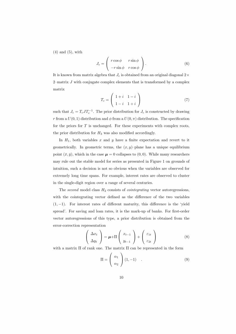
(4) and (5), with

Jc =

r cosφ r sinφ

−r sinφ r cosφ

. (6)

It is known from matrix algebra that Jc is obtained from an original diagonal 2×2�matrix J with conjugate complex elements that is transformed by a complex

matrix

Tc =

1 + i 1− i1− i 1 + i

(7)

such that Jc = TcJT−1c . The prior distribution for Jc is constructed by drawing

r from a U(0, 1) distribution and φ from a U(0,π) distribution. The speciÞcation

for the priors for T is unchanged. For these experiments with complex roots,

the prior distribution for H3 was also modiÞed accordingly.

In H1, both variables x and y have a Þnite expectation and revert to it

geometrically. In geometric terms, the (x, y)�plane has a unique equilibrium

point (x, y), which in the case µ = 0 collapses to (0, 0). While many researchers

may rule out the stable model for series as presented in Figure 1 on grounds of

intuition, such a decision is not so obvious when the variables are observed for

extremely long time spans. For example, interest rates are observed to cluster

in the single-digit region over a range of several centuries.

The second model class H2 consists of cointegrating vector autoregressions,

with the cointegrating vector deÞned as the difference of the two variables

(1,−1). For interest rates of different maturity, this difference is the �yield

spread�. For saving and loan rates, it is the mark-up of banks. For Þrst-order

vector autoregressions of this type, a prior distribution is obtained from the

error-correction representation ∆xt

∆yt

= µ+Π

xt−1

yt−1

+ ε1t

ε2t

(8)

with a matrix Π of rank one. The matrix Π can be represented in the form

Π =

α1

α2

(1,−1) . (9)

10

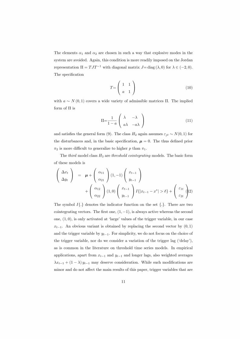
The elements α1 and α2 are chosen in such a way that explosive modes in the

system are avoided. Again, this condition is more readily imposed on the Jordan

representation Π = TJT−1 with diagonal matrix J=diag (λ, 0) for λ ∈ (−2, 0).The speciÞcation

T=

1 1

a 1

(10)

with a ∼ N (0, 1) covers a wide variety of admissible matrices Π. The impliedform of Π is

Π=1

1− a

λ −λaλ −aλ

(11)

and satisÞes the general form (9). The class H2 again assumes εjt ∼ N(0, 1) forthe disturbances and, in the basic speciÞcation, µ = 0. The thus deÞned prior

π2 is more difficult to generalize to higher p than π1.

The third model class H3 are threshold cointegrating models. The basic form

of these models is ∆xt

∆yt

= µ+

α11

α21

(1,−1) xt−1

yt−1

+

α12

α22

(1, 0) xt−1

yt−1

I{|xt−1 − x∗| > δ}+ ε1t

ε2t

.(12)The symbol I{.} denotes the indicator function on the set {.}. There are twocointegrating vectors. The Þrst one, (1,−1), is always active whereas the secondone, (1, 0), is only activated at �large� values of the trigger variable, in our case

xt−1. An obvious variant is obtained by replacing the second vector by (0, 1)

and the trigger variable by yt−1. For simplicity, we do not focus on the choice of

the trigger variable, nor do we consider a variation of the trigger lag (�delay�),

as is common in the literature on threshold time series models. In empirical

applications, apart from xt−1 and yt−1 and longer lags, also weighted averages

λxt−1 + (1− λ) yt−1 may deserve consideration. While such modiÞcations areminor and do not affect the main results of this paper, trigger variables that are

11

stationary under H2, such as ∆xt−1 or xt−1−yt−1, change the properties of H3and cannot be treated in the presented framework.

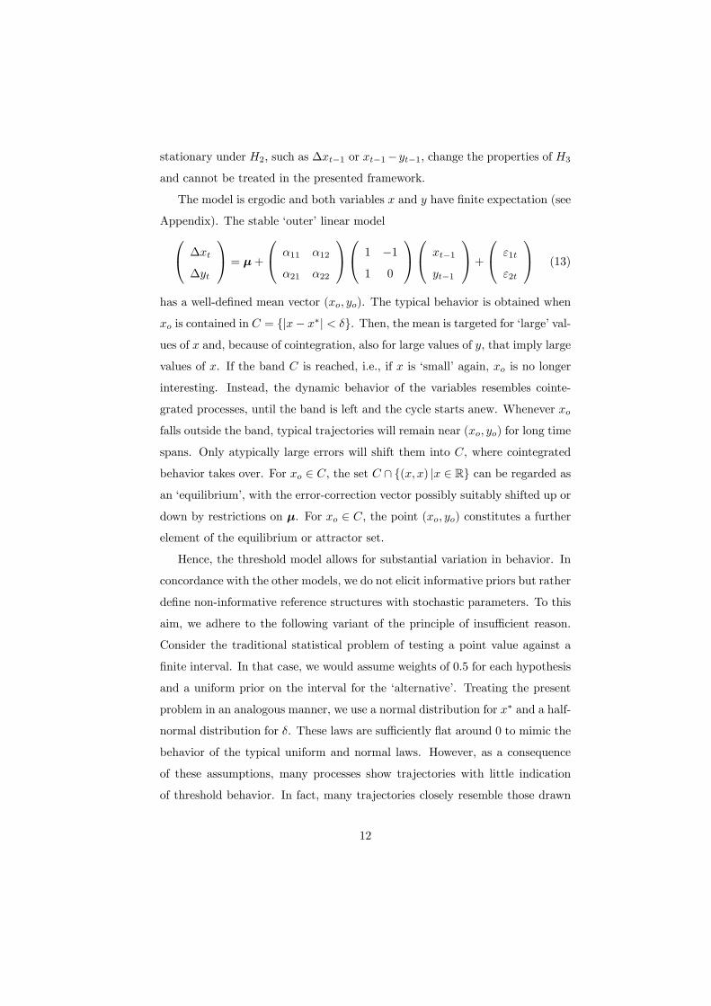
The model is ergodic and both variables x and y have Þnite expectation (see

Appendix). The stable �outer� linear model ∆xt

∆yt

= µ+

α11 α12

α21 α22

1 −11 0

xt−1

yt−1

+ ε1t

ε2t

(13)

has a well-deÞned mean vector (xo, yo). The typical behavior is obtained when

xo is contained in C = {|x− x∗| < δ}. Then, the mean is targeted for �large� val-ues of x and, because of cointegration, also for large values of y, that imply large

values of x. If the band C is reached, i.e., if x is �small� again, xo is no longer

interesting. Instead, the dynamic behavior of the variables resembles cointe-

grated processes, until the band is left and the cycle starts anew. Whenever xo

falls outside the band, typical trajectories will remain near (xo, yo) for long time

spans. Only atypically large errors will shift them into C, where cointegrated

behavior takes over. For xo ∈ C, the set C ∩ {(x, x) |x ∈ R} can be regarded asan �equilibrium�, with the error-correction vector possibly suitably shifted up or

down by restrictions on µ. For xo ∈ C, the point (xo, yo) constitutes a furtherelement of the equilibrium or attractor set.

Hence, the threshold model allows for substantial variation in behavior. In

concordance with the other models, we do not elicit informative priors but rather

deÞne non-informative reference structures with stochastic parameters. To this

aim, we adhere to the following variant of the principle of insufficient reason.

Consider the traditional statistical problem of testing a point value against a

Þnite interval. In that case, we would assume weights of 0.5 for each hypothesis

and a uniform prior on the interval for the �alternative�. Treating the present

problem in an analogous manner, we use a normal distribution for x∗ and a half-

normal distribution for δ. These laws are sufficiently ßat around 0 to mimic the

behavior of the typical uniform and normal laws. However, as a consequence

of these assumptions, many processes show trajectories with little indication

of threshold behavior. In fact, many trajectories closely resemble those drawn

12

from H1. �Non-revealing� trajectories occur if the threshold criterion is never

activated in the assumed sample length. Statistical criteria cannot be expected

to classify such cases correctly. Thus, it may be more difficult to discriminate

H3 from H1 ∪H2 than to discriminate between H1 and H2.

2.3 The discriminatory statistics

In order to discriminate among the three candidate models, two discriminatory

statistics were employed. The statistic S2 is designed to be powerful in discrim-

inating H1 and H2. In the notation of section 2.1, it would be labelled S21. S2

is deÞned as the smaller canonical root for (∆xt,∆yt) and (xt−1, yt−1). As Jo-

hansen (1995) pointed out, this root makes part of the likelihood-ratio test for

hypotheses that concern the cointegrating rank of vector autoregressions. If the

larger canonical root is zero, (x, y) forms a bivariate integrated process without

a stable mode. If only the smaller canonical root is zero, (x, y) is a cointegrated

process with a stationary linear combination β1x+β2y. If the smaller canonical

root is also non-zero, (x, y) is a stationary process with all modes being stable.

Because the rank-zero model is not acceptable for the investigated data, only

the smaller root is in focus.

An alternative statistic to S2 would be a variant that uses the information

on the potential cointegrating vector (1,−1). While that statistic would bemore powerful in discriminating H1 and H2 in the given form, we feel that some

ßexibility regarding the exact form of the equilibrium vector is appropriate. In

other words, the decision maker is not supposed to know the vector exactly.

The statistic to appear on the x�axis, S1, is designed to discriminate H1 and

H3. In the notation of section 2.1, it would be labelled S13, though it may also

be useful in discriminating H2 and H3. S1 is an approximate likelihood-ratio

test statistic for the stationary vector autoregression H1 versus the quite spe-

cial threshold-cointegrating model with δ and x∗ being determined over a grid

of fractiles of x. In detail, δ is varied from the halved interquartile range to

the halved distance between the empirical 0.05 and 0.95 fractiles, with x∗ thus

13

assumed in the center of the range. For assumed models of type (12), the error

sum of squares is minimized over a grid with step size of 0.05. As T →∞, thisgrid should be reÞned. Conditional on x∗ and δ, estimating (12) is an ordinary

least-squares problem with a corresponding residual covariance, whose log deter-

minant can be compared to that of the unrestricted linear autoregression. The

residual under the assumption of model class Hj is denoted by �ε(j)t . For j = 1, 2,

this residual is calculated using the maximum-likelihood estimator. For j = 3,

the approximate maximum likelihood estimator over the outlined grid is used.

The residual covariance matrix is denoted by �Σj = T−1PT

t=1 �ε(j)t �ε

(j)0t . With

this notation, the second statistic is deÞned as S1 = ln³det �Σ3

´− ln

³det �Σ1

´.

Note that S1 can be positive or negative. S1 < 0 for strong nonlinear

threshold effects, as H3 attains a better Þt. S1 > 0 for stable autoregres-

sions. The hypotheses H1 and H3 are not nested. The statistic S1 optimizes

the likelihood ratio over a limited range, which is the prevalent approach for

nonlinearity testing (see, e.g., Caner and Hansen, 2001). An alternative is

the semi-parametric test by Tsay (1998) that relies on sorting the observations

according to the source of nonlinearity. The fully parametric nature of our de-

cision problem, however, suggests the use of S1. Another alternative would be

a likelihood ratio S23, which may be motivated by the fact that the hypotheses

H2 and H3 are nested. We do not consider S23, as it is an unusual statistic

whose properties have not been fully explored.

The null fractiles were generated as follows. For S2, Jordan priors were

used on a cointegrating autoregression�the classical lower-dimensional �null�

hypothesis H2. The cointegrating rank was Þxed at one, whereas the cointe-

grating vector was not speciÞed in constructing S2. The null fractiles differ from

those that were tabulated by Johansen (1995), as those were calculated under

the hypothesis of multivariate random walks. For S1, Jordan priors on stable

vector autoregressions were used, according to the classical �null� hypothesis H1.

14

2.4 Smoothing

The technique of discretizing the statistics in bins corresponds to a rectangular

smoothing kernel in density estimation. Similarly, simulated boundaries of the

decision areas often have a rough appearance, even for a high number of repli-

cations. It was found that smoothing the original numbers in the bins across

neighboring bins is not as reliable as smoothing approximate posterior probabil-

ities for the hypotheses. This effect is probably due to the scaling of numbers.

As a smoothing kernel, an inverse absolute function

w (i, j) =W

1 + |i− i0|+ |j − j0| , i0 − nw ≤ i ≤ i0 + nw,j0 − nw ≤ j ≤ j0 + nw (14)

was used over an (2nw + 1) × (2nw + 1) submatrix of the complete matrix ofbins. This submatrix is centered at the location (i0, j0), where the value is to

be estimated. W is set such that the sum of kernel weightsPw(i, j) over the

submatrix equals one. Generally, the number nw was selected as the minimum

number, at which smooth boundary curves were obtained. The maps show some

deliberate variation of nw, in order to demonstrate its inßuence on the results.

3 Simulation results: the maps

Figures 2 and 3 show decision maps resulting from 3×106 simulations of processtrajectories of length T = 50 with stochastic parameters according to the prior

distributions that were described in Section 2.2, i.e., 106 simulations for each

model. These basic simulations use the simpliÞed priors with µ = 0. In Figure

2, no smoothing was performed (nw = 0), while Figure 3 used nw = 3. One sees

that the main effect of smoothing is a better separation of the preference areas

for H1 and H3, which is mainly achieved by eliminating the scattered preference

specks for the rather inhomogeneous hypothesis H3. Further increases of nw

distort the main boundaries of H1 and H2 and of H1 and H3.

The main features of the decision map are somewhat surprising. The thresh-

old statistic S1 appears to be valuable in discriminating cointegrated and stable

15

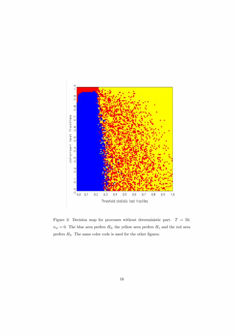
Figure 2: Decision map for processes without deterministic part. T = 50,

nw = 0. The blue area prefers H2, the yellow area prefers H1 and the red area

prefers H3. The same color code is used for the other Þgures.

16

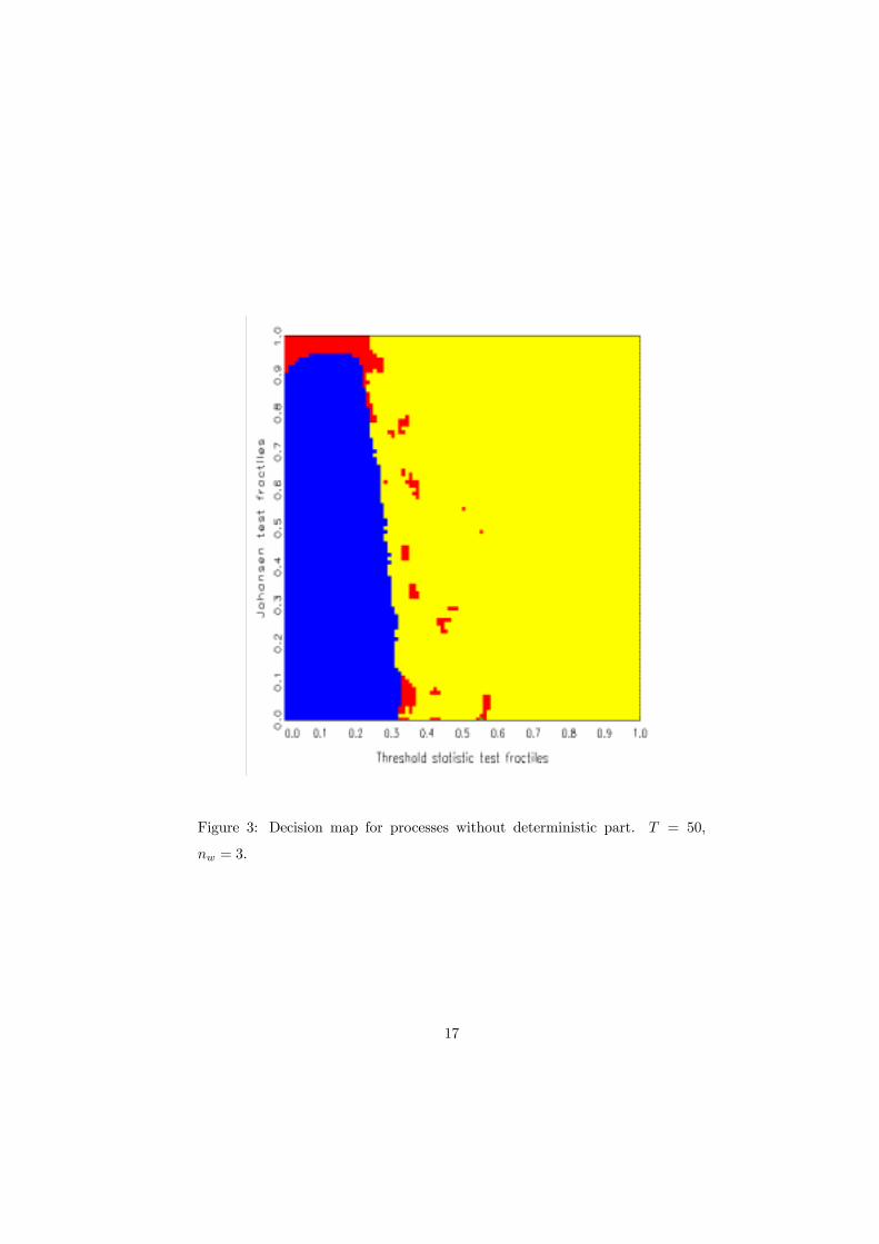
Figure 3: Decision map for processes without deterministic part. T = 50,

nw = 3.

17

models, while it was designed to point out threshold structures. The Johansen-

type statistic S2 separates linear cointegrated models from cases of threshold

cointegration, while it was designed to test for potential cointegration in stable

vector autoregressions. A closer look reveals that H3 models are indeed char-

acterized by small values of S1, as expected, and hence are most numerous in

the left part of the chart. However, H2 models also incur small values of the

statistic S1, as a threshold structure with the critical value pushed away from

the starting values will achieve a better Þt to data than an unrestricted vector

autoregression for cointegrated models. In other words, linear cointegration re-

sults as a limiting case of threshold cointegration. The posterior probability for

H2 is more concentrated than that for H3, hence H2 dominates the left part

of the diagram. Similarly, rejection of the smaller canonical root being zero

may point to a stable linear model without unit roots but it may also point

to a threshold model, which is stationary and ergodic though non-linear. The

joint evidence of two non-zero canonical roots and a better Þt by a restricted

structure yields the preference area for H3 in the north-west.

The map implies a crude empirical guideline. First, use the threshold statis-

tic S1. For values larger than the 0.3 fractile, a linear stable model is suggested.

For smaller values, use the lesser canonical root S2. If this root is �signiÞcant�

at 0.05, consider the threshold model, otherwise opt for linear cointegration.

In Figure 4, the sample size has increased to T = 100, while the other

simulation parameters were retained. The smoothing bandwidth was kept at

nw = 3. The nominal signiÞcance level of the canonical root has decreased

to 0.02, whereas the critical fractile of the threshold statistic decreases to 0.2.

These features are in line with expectations regarding large-sample performance.

There is now more evidence on a preference for threshold models in a wedge

between the other two models, i.e., for threshold statistics in the fractile range

(0.2, 0.3), particularly if S2 is �not too small�. The scattered appearance of the

H3 area reßects the varying shape of trajectories of length T = 100, which

generally does not permit a safe classiÞcation. Many of these H3 trajectories

are indeed very similar or identical to H1 trajectories from the stable model

18

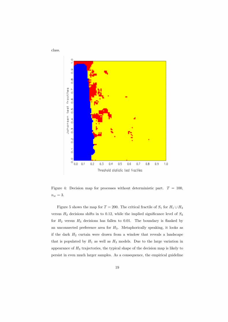
class.

Figure 4: Decision map for processes without deterministic part. T = 100,

nw = 3.

Figure 5 shows the map for T = 200. The critical fractile of S1 for H1 ∪H3versus H2 decisions shifts in to 0.12, while the implied signiÞcance level of S2

for H2 versus H3 decisions has fallen to 0.01. The boundary is ßanked by

an unconnected preference area for H3. Metaphorically speaking, it looks as

if the dark H2 curtain were drawn from a window that reveals a landscape

that is populated by H1 as well as H3 models. Due to the large variation in

appearance of H3 trajectories, the typical shape of the decision map is likely to

persist in even much larger samples. As a consequence, the empirical guideline

19

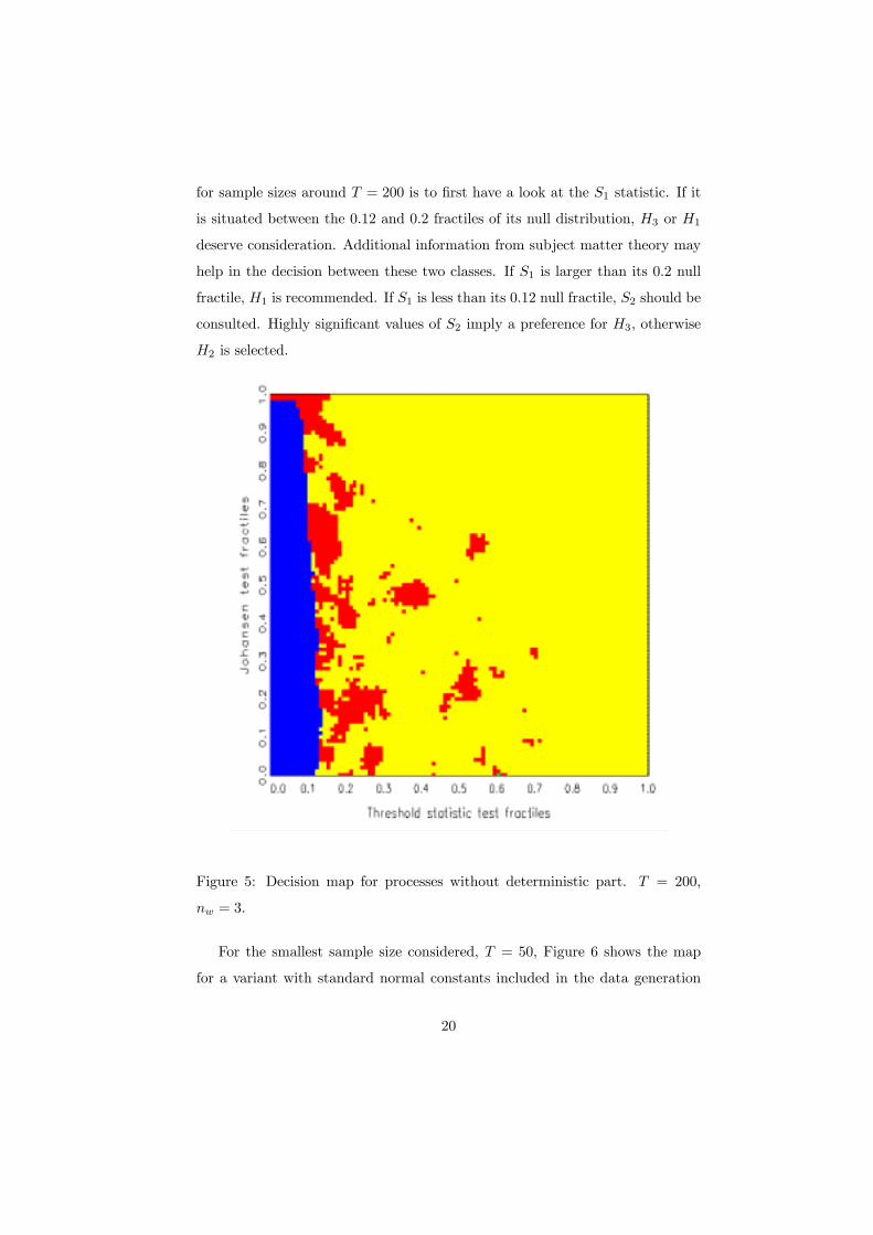
for sample sizes around T = 200 is to Þrst have a look at the S1 statistic. If it

is situated between the 0.12 and 0.2 fractiles of its null distribution, H3 or H1

deserve consideration. Additional information from subject matter theory may

help in the decision between these two classes. If S1 is larger than its 0.2 null

fractile, H1 is recommended. If S1 is less than its 0.12 null fractile, S2 should be

consulted. Highly signiÞcant values of S2 imply a preference for H3, otherwise

H2 is selected.

Figure 5: Decision map for processes without deterministic part. T = 200,

nw = 3.

For the smallest sample size considered, T = 50, Figure 6 shows the map

for a variant with standard normal constants included in the data generation

20

mechanism. The assumption µ = 0 in (3), (6), (10) was replaced by µ~N(0, I2).

The existence of a constant was also assumed in calculating the statistics S1 and

S2. The effects of this intercept are different for each hypothesis. In H1, only

the mean is affected. In H2, a linear trend is added. In H3, a linear trend is

generated within the inner regime. These asymmetric effects tend to simplify

decisions between the model classes. Hence, the vertical boundary of the H2

preference area is to the left of the comparable one in Figure 3. The critical

fractile for this decision is around 0.1. The preference area for threshold models

H3 has grown considerably and shows a connected pattern in the upper part of

the map between the 0.1 and 0.3 fractiles of S1. The inßuence of the canonical

root S2 on the decision has disappeared with respect to the H2 class and is

rather secondary for the H1 versus H3 decision. As a rough guideline, this

map suggests that threshold cointegration should be considered whenever S1 is

between its lower decile and lower quartile and S2 is not in its lower tail. It is

difficult to explain the H3 preference in the north-east corner or the S�shape in

the right-hand boundary of the main H3 preference area. These features may

be caused by speciÞc properties of the prior distributions or may be artifacts.

For T = 100, the map of Figure 7 is obtained. The critical fractile of S1

for the decision H1 ∪H3 versus H2 has shifted in to about 0.05. By contrast,the boundary between the preference areas for H1 and H3 has hardly changed.

The effect of the �drawn curtain� is felt again, such that the H3 preference area

stretches down to the x�axis, i.e., to low S2 values. The spot in the north-east

persists. The asymptotic behavior suggested by Figure 7 is corroborated for

T = 200 in Figure 8. The critical fractile for the S1 statistic and the H2 versus

H1 ∪H3 areas decreases to 0.03, whereas the boundary between the hypothesesH1 and H3 remains in place. In this setup, hypothesis H2 corresponds to the

only transient model, which simpliÞes its detection in larger samples. Contrary

to what may be an intuitive assumption, discriminating threshold structures

from linear autoregressions is not automatically simpliÞed as T → ∞. Note,however, that the resolution of the grid and the range for the grid search were

kept constant. For asymptotic properties such as consistency, such parameters

21

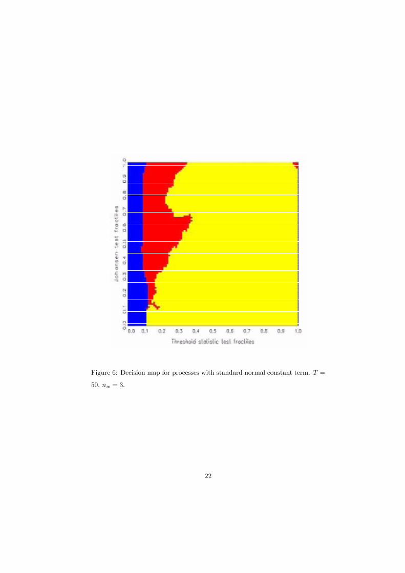
Figure 6: Decision map for processes with standard normal constant term. T =

50, nw = 3.

22

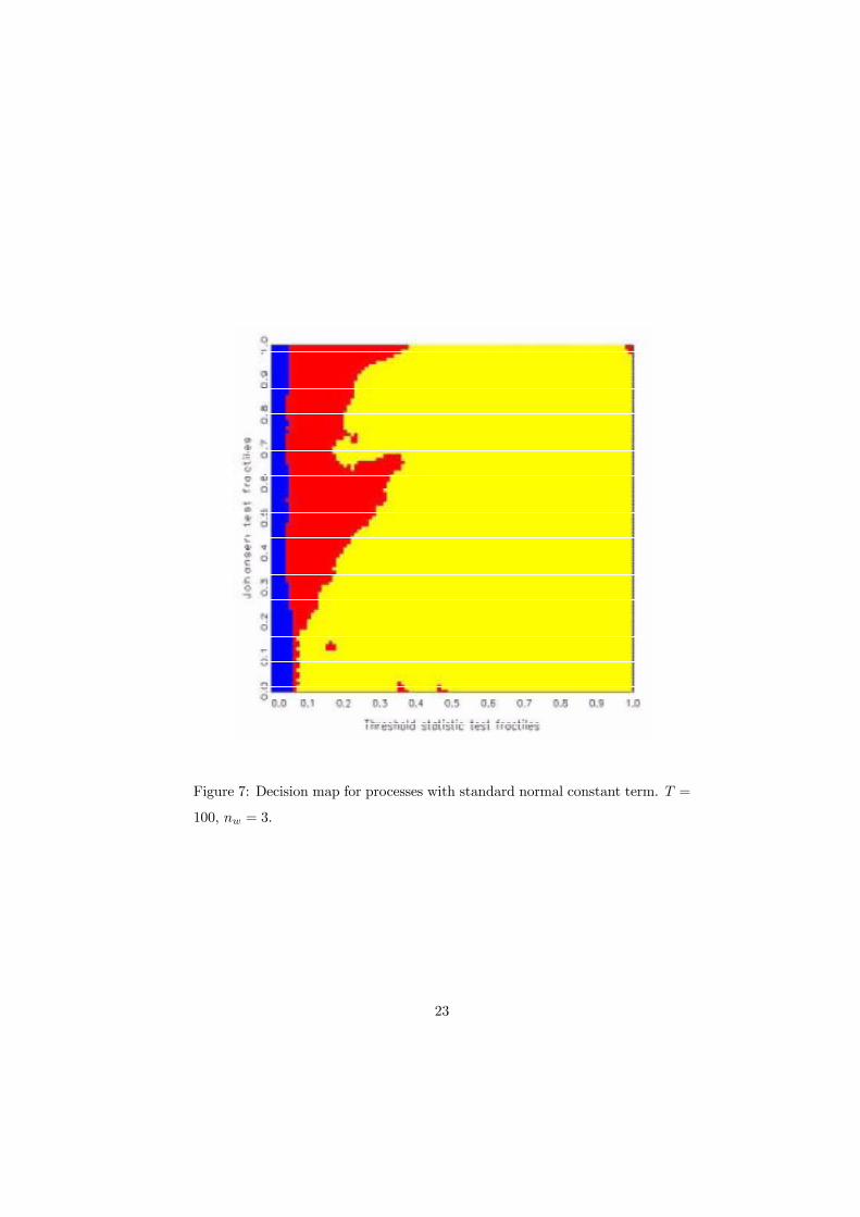
Figure 7: Decision map for processes with standard normal constant term. T =

100, nw = 3.

23

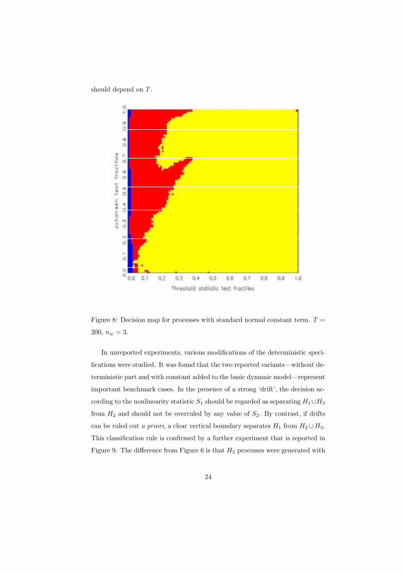
should depend on T .

Figure 8: Decision map for processes with standard normal constant term. T =

200, nw = 3.

In unreported experiments, various modiÞcations of the deterministic speci-

Þcations were studied. It was found that the two reported variants�without de-

terministic part and with constant added to the basic dynamic model�represent

important benchmark cases. In the presence of a strong �drift�, the decision ac-

cording to the nonlinearity statistic S1 should be regarded as separatingH1∪H3from H2 and should not be overruled by any value of S2. By contrast, if drifts

can be ruled out a priori, a clear vertical boundary separates H1 from H2 ∪H3.This classiÞcation rule is conÞrmed by a further experiment that is reported in

Figure 9. The difference from Figure 6 is that H2 processes were generated with

24

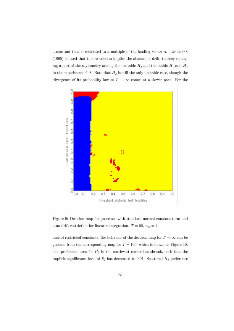
a constant that is restricted to a multiple of the loading vector α. Johansen

(1995) showed that this restriction implies the absence of drift, thereby remov-

ing a part of the asymmetry among the unstable H2 and the stable H1 and H3

in the experiments 6�8. Note that H2 is still the only unstable case, though the

divergence of its probability law as T → ∞ comes at a slower pace. For the

Figure 9: Decision map for processes with standard normal constant term and

a no-drift restriction for linear cointegration. T = 50, nw = 4.

case of restricted constants, the behavior of the decision map for T →∞ can be

guessed from the corresponding map for T = 100, which is shown as Figure 10.

The preference area for H3 in the northwest corner has shrunk, such that the

implicit signiÞcance level of S2 has decreased to 0.01. Scattered H3 preference

25

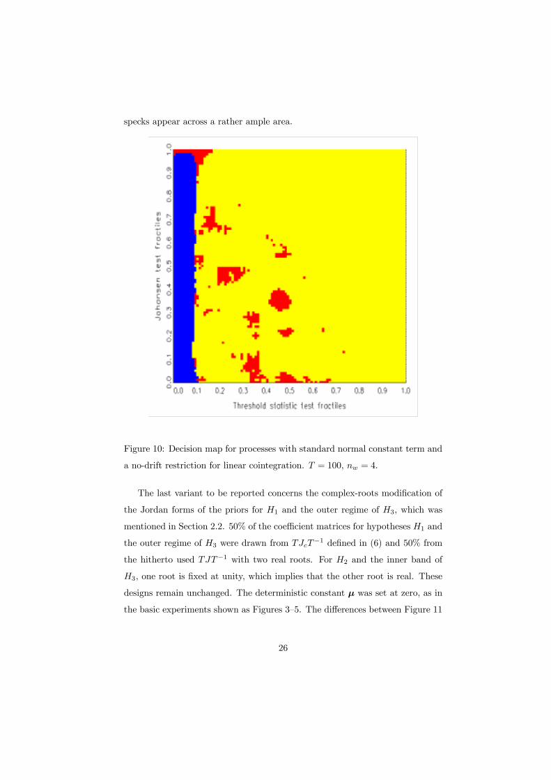
specks appear across a rather ample area.

Figure 10: Decision map for processes with standard normal constant term and

a no-drift restriction for linear cointegration. T = 100, nw = 4.

The last variant to be reported concerns the complex-roots modiÞcation of

the Jordan forms of the priors for H1 and the outer regime of H3, which was

mentioned in Section 2.2. 50% of the coefficient matrices for hypotheses H1 and

the outer regime of H3 were drawn from TJcT−1 deÞned in (6) and 50% from

the hitherto used TJT−1 with two real roots. For H2 and the inner band of

H3, one root is Þxed at unity, which implies that the other root is real. These

designs remain unchanged. The deterministic constant µ was set at zero, as in

the basic experiments shown as Figures 3�5. The differences between Figure 11

26

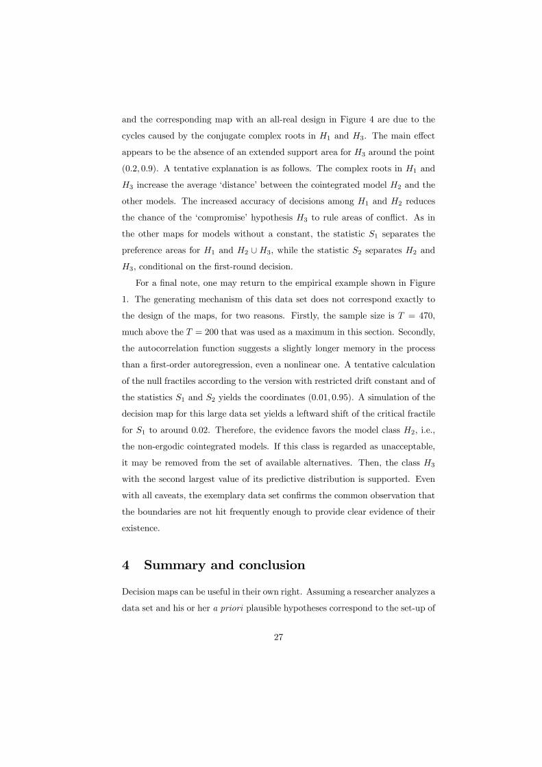
and the corresponding map with an all-real design in Figure 4 are due to the

cycles caused by the conjugate complex roots in H1 and H3. The main effect

appears to be the absence of an extended support area for H3 around the point

(0.2, 0.9). A tentative explanation is as follows. The complex roots in H1 and

H3 increase the average �distance� between the cointegrated model H2 and the

other models. The increased accuracy of decisions among H1 and H2 reduces

the chance of the �compromise� hypothesis H3 to rule areas of conßict. As in

the other maps for models without a constant, the statistic S1 separates the

preference areas for H1 and H2 ∪ H3, while the statistic S2 separates H2 andH3, conditional on the Þrst-round decision.

For a Þnal note, one may return to the empirical example shown in Figure

1. The generating mechanism of this data set does not correspond exactly to

the design of the maps, for two reasons. Firstly, the sample size is T = 470,

much above the T = 200 that was used as a maximum in this section. Secondly,

the autocorrelation function suggests a slightly longer memory in the process

than a Þrst-order autoregression, even a nonlinear one. A tentative calculation

of the null fractiles according to the version with restricted drift constant and of

the statistics S1 and S2 yields the coordinates (0.01, 0.95). A simulation of the

decision map for this large data set yields a leftward shift of the critical fractile

for S1 to around 0.02. Therefore, the evidence favors the model class H2, i.e.,

the non-ergodic cointegrated models. If this class is regarded as unacceptable,

it may be removed from the set of available alternatives. Then, the class H3

with the second largest value of its predictive distribution is supported. Even

with all caveats, the exemplary data set conÞrms the common observation that

the boundaries are not hit frequently enough to provide clear evidence of their

existence.

4 Summary and conclusion

Decision maps can be useful in their own right. Assuming a researcher analyzes a

data set and his or her a priori plausible hypotheses correspond to the set-up of

27

Figure 11: Decision map for processes with zero constant and a 0.5 chance of

conjugate complex roots in stable autoregressive coefficient matrices. T = 100,

nw = 3.

28

the decision map simulation. If the coordinates of the decision map are available,

two statistics S1 and S2 can quickly be calculated from the data and can be

encoded as null fractiles. Otherwise, a simulation may be used for performing

the encoding. In the map, preference areas for the conßicting hypotheses are

clearly separated by boundaries.

Decision maps are, however, even more important as summary guidelines

for the empirical researcher. Vertical or almost vertical boundaries indicate

that relying on S1 is almost as valuable for discriminating the hypotheses as

the joint evaluation of S1 and S2. Similarly, horizontal boundaries underscore

the value of S2 relative to S1. In the present experiments, it was found that

the main discriminatory power rests on the threshold statistic S1, not only

among hypotheses H1 and H2, i.e., stationarity and cointegration. Correct

identiÞcation of threshold models turned out to be extremely difficult even for

relatively large samples such as T = 200. This difficulty is corroborated by

tentatively removing H2 from the set of available hypotheses. The implied map

shows that H2 and H3 approximately dominate the same area, a vertical band,

with H2 more concentrated there. Formally, the decision maps suggest decisions

for H3 around the boundary between the preference areas for the other two

hypotheses, i.e., for S1 values around the �critical values�. Another preference

area for H3 is the more �natural� one in the northwest corner, where S2 is in

the upper tail of its null distribution. The empirical recommendation by some

authors (see Lo and Zivot, 2001) to test for cointegration in a linear frame

Þrst and then to check for nonlinearity is not generally conÞrmed. Rather,

the maps recommend to test for nonlinearity Þrst. Structures with sufficiently

large values of S1 are classiÞed as stationary H1 models. As a second step, a

cointegration test is conducted. If cointegration is rejected for a model classiÞed

as �nonlinear�, a threshold model H3 is indicated. If cointegration cannot be

rejected, a cointegrated linear model H2 is supported. Traditional simulation

with Þxed parametric designs could never unveil this general decision pattern.

The unconnected specks of preference for H3 reßect the fact that threshold

processes generate two species of trajectories: typical trajectories with statistics

29

clustered in the northwest region and atypical trajectories with hardly recog-

nizable threshold effects and statistics almost anywhere in the left part of thee

[0, 1] × [0, 1]�plane. Most atypical trajectories stem from designs with small

values of δ and therefore roughly �look like� trajectories from stationary autore-

gressions. The high risk of incorrectly classifying the generating processes as H1

may incur a relatively modest risk if one proceeds with the incorrect model, as

the linear model may be a good workhorse for typical econometric tasks such as

prediction. A careful evaluation of this conjecture is a promising task for future

work.

Many researchers may be skeptical about the usage of decision maps, partic-

ularly when the dynamic speciÞcation of short-run nuisance for Hj , j = 1, . . . , 3

is slightly simpler than time-series structures that prevail in the literature. In

order to counter this argument, more sophisticated priors must be introduced,

which unfortunately entails a considerable increase in computer time. For an

example of higher-order autoregressions and elements of lag order search via in-

formation criteria within the decision-maps framework, see Kunst (2001). Such

extensions are possible directions for future research.

Acknowledgments

The data on U.S. interest rates are taken from the International Financial Sta-

tistics database. The author thanks Manfred Deistler, Elizaveta Krylova, Sylvia

Kaufmann, and an anonymous referee for helpful comments, and Elizabeth Raab

for proofreading. The usual proviso applies.

Appendix: Geometric ergodicity of threshold coin-

tegrated models

The recent econometric literature on threshold cointegrated models offers no

formal proof of the stability properties of threshold cointegrated models with

30

stable outer regimes. For the variant that is used as hypothesis H3 in the paper,

such proof is provided here.

The �threshold cointegration model� is deÞned as the nonlinear Þrst-order

autoregressive structure ∆xt

∆yt

= αβ0

xt−1

yt−1

+ γ1

γ2

xt−1I (|xt−1 − x∗| > δ) + εt . (15)

For simplicity, no deterministic terms are used except for the x center x∗. The

model is equivalent to a stable autoregression for the outer region {|xt−1−x∗| >δ} and to a cointegrating partial stable autoregression for the inner region. Weassume the following conditions:

A1: The polynomial det{I2−¡I2 +αβ

0¢ z} has no roots inside the unit circleor for |z| = 1 but z 6= 1. The second-order matrix condition for the Granger rep-resentation theorem (see Engle and Granger, 1987, and Johansen, 1995)

detα0⊥β⊥ 6= 0 applies, where the subscript ⊥ denotes the orthogonal comple-

ment.

A2: The polynomial det{I2 −¡I2 +αβ

0 + γe01¢} has all roots outside the

unit circle, where e1 = (1, 0)0.

For the errors εt a regularity condition is assumed:

A3: The distribution of the errors εt is absolutely continuous and strictly

positive on R2.

Conditions A1 and A2 guarantee that the model corresponds to the above

concept, with A1 essentially due to Engle and Granger (1987) and to Jo-

hansen (1988) and A2 a standard assumption of time series analysis. Given

A1, note that A2 restricts γ and excludes β = (λ, 0)0 for arbitrary λ 6= 0. A3implies irreducibility and aperiodicity for all threshold autoregressive models.

With these assumptions, the following result by Tong (1990, p. 457) can be

applied:

Theorem 1 (Drift criterion, Tong) Let {Zt} be aperiodic and irreducible.Suppose a small set C exists, a non-negative measurable function g, and con-

31

stants r > 1, γ > 0, and B > 0 such that

E{rg (Zt+1) |Zt = z} < g(z)− γ, z /∈ C (16)

and

E{g (Zt+1) |Zt = z} < B, z ∈ C. (17)

Then, {Zt} is geometrically ergodic.

The small set C is meant to contain the �center� of the stationary distribution,

assuming its existence. For a Þrst-order autoregression with stable coefficient,

the condition (16) holds for any subset of R2 outside the mean, that is, outside

a disk around zero if there are no deterministic terms. For the deÞnition of a

small set, see Tong (1990, p. 454). A technical complication is to prove that

compact sets are small. For all nonlinear autoregressions of the threshold type,

this can be shown as in Chan et al. (1985). This result implies the following.

Theorem 2 Let Zt = (xt, yt)0 for t > 0 obey the model (15) with the condi-

tions A1�A3 and arbitrary Þxed starting conditions. Then, {Zt} is geometricallyergodic.

Proof: Decompose the space R2 into Þve disjoint areas such that R2 =

∪5j=1Aj . We analyze all of them in turn.

1. A1 = {x < x∗ − δ} The process is locally geometric stable and condition(16) is fulÞlled for many functions g (z), among them all absolute values

of linear functions in the arguments x and y, provided that the implied

mean of the autoregression Zt =¡I2 +αβ

0 + γe01¢Zt−1 + εt is outside

A1. The maximum eigenvalue λ of the regressor matrix is less than one

in modulus because of A2, hence any value λ0 in the open interval (|λ|, 1)can be chosen for 1/r. γ can be set to (λ0 − λ)min{g(z)|z ∈ A1}. If theimplied mean µ is inside A1, the proof must be formulated with respect

to A∗1 = {x < x∗∗ − δ} for x∗∗ being the x�component of µ. The areaA∗1 −A1 is appropriately allotted to A3 ∪A4 ∪A5.

32

2. A2 = {x > x∗ + δ} Same as A1. Again, A2 may be replaced by A∗2 ifnecessary.

3. A3 = {|x − x∗| < δ and |y| < K} with K chosen large enough that the

inner equilibrium line segment β0 (x, y)0 is fully contained in A3. Note that

this construction assumes that the second element of β is non-zero, which

is excluded by assumption A2, as the system given in A2 and deÞned

by the �outer regime� cannot become stable if both cointegrating vectors

coincide. Clearly, condition (17) is fulÞlled. The implication is unaffected

by the change from A1 to A∗1 and the implied change of A3 to A∗3. To

show that A3 is small under the assumptions A1�A3, we refer to Tong

(1990) who states that, for locally linear models with error distributions

satisfying A3, all compact sets are small.

4. A4 = {|x − x∗| < δ and y > K}. DeÞning g(x) as the distance to theequilibrium line segment, for example in the Euclidean metric, yields con-

dition (16) for this area. This function is also valid for A1 and A2. The

implication is unaffected by the change from Aj to A∗j for j = 1, . . . , 5.

5. A5 = {|x− x∗| < δ and y < K}. Same as A4.

A3 is small in the sense of Theorem 1, which completes the proof.¥Note that Theorem 2 gives no result for the case that the inner regime does

not cointegrate. In fact, then �probability mass escapes�, as trajectories may

wander in the direction of the unrestricted variable y. The result by Chan et

al. (1985) does not generalize to the multivariate case immediately, when the

inner area is not completely bounded. A similar observation holds with respect

to the degenerate case where the equilibrium line segment is vertical in the

sense that β = (λ, 0)0. Obviously, the proof is unaffected by changing the signal

variable x to y or to any linear combination of x and y different from β0X.

33

References

[1] Backus, D.K. and Zin, S.E. (1993) �Long-Memory Inßation Uncertainty:

Evidence from the Term Structure of Interest Rates� Journal of Money,

Credit, and Banking 25, 681�700.

[2] Balke, N.S. and Fomby, T.B. (1997) �Threshold Cointegration� Inter-

national Economic Review 38, 627�645.

[3] Bauwens, L., Lubrano, M. and Richard, J.-F. (1999) Bayesian In-

ference in Dynamic Econometric Models. Oxford University Press.

[4] Berger, J.O. and Yang, R.Y. (1994) �Non-informative priors and

Bayesian testing for the AR(1) model� Econometric Theory 10, 461�482.

[5] Campbell, J.Y. and Shiller, R.J. (1987) �Cointegration and Tests of

Present Value Models� Journal of Political Economy 95, 1062�1088.

[6] Caner, M., and Hansen, B.E. (2001) �Threshold Autoregression with a

Unit Root� Econometrica 69, 1555�1596.

[7] Chan, K.S. (1993) �Consistency and limiting distribution of the least

squares estimator of a threshold autoregressive model� Annals of Statis-

tics 21, 520�533.

[8] Chan, K.S., Petruccelli, J.D., Tong, H. and Woolford, S.W.

(1985) �A multiple threshold AR(1) model� Annals of Applied Probability

22, 267�279.

[9] Chan, K.S. and Tsay, R. (1998) �Limiting properties of the least squares

estimator of a continuous threshold autoregressive model� Biometrika 85,

413�426.

[10] Enders, W. and Falk, B. (1998) �Threshold-autoregressive, median-

unbiased, and cointegration tests of purchasing power parity� International

Journal of Forecasting 14, 171�186.

34

[11] Enders, W. and Granger, C.W.J. (1998) �Unit-root tests and asym-

metric adjustment with an example using the term structure of interest

rates� Journal of Business and Economic Statistics 16, 304�311.

[12] Enders, W. and Siklos, P. (2001) �Cointegration and Threshold Ad-

justment� Journal of Business and Economic Statistics 19, 166�176.

[13] Engle, R.F. and Granger, C.W.J. (1987) �Co-integration and Error

Correction: Representation, Estimation, and Testing� Econometrica 55,

251�276.

[14] Hall, A.D., Anderson, H.M. and Granger , C.W.J.(1992) �A Cointe-

gration Analysis of Treasury Bill Yields� Review of Economics and Statistics

74, 116�126.

[15] Hansen, B.E. and Seo, B. (2002) �Testing for two-regime threshold coin-

tegration in vector error-correction models� Journal of Econometrics, forth-

coming.

[16] Hatanaka, M. (1996) Time-Series-Based Econometrics: Unit Roots and

Co-Integration. Oxford University Press.

[17] Johansen, S. (1988) �Statistical analysis of cointegration vectors� Journal

of Economic Dynamics and Control 12, 231�254.

[18] Johansen, S. (1995) Likelihood-Based Inference in Cointegrated Vector

Autoregressive Models. Oxford University Press.

[19] Johansen, S. and Juselius, K. (1992) �Testing Structural Hypotheses

in a Multivariate Cointegration Analysis of the PPP and the UIP for the

UK� Journal of Econometrics 53, pages 211�244.

[20] Jumah, A. and Kunst, R.M. (2002) �On mean reversion in real interest

rates: An application of threshold cointegration� Economics Series No. 109,

Institute for Advanced Studies, Vienna.

35

[21] Kunst, R.M. (2001) �Testing for stationarity in a cointegrated system�

Paper presented at the Econometric Society European Meeting, August

2001, Lausanne.

[22] Kunst, R.M. and Reutter, M. (2002) �Decisions on seasonal unit roots�

Journal of Statistical Computation and Simulation 72, 403-418.

[23] Lo, M.C. and Zivot, E. (2001) �Threshold cointegration and nonlinear

adjustment to the law of one price� Macroeconomic Dynamics 5, 533�576.

[24] Tong, H. (1990) Non-linear time series: a dynamical system approach.

Oxford University Press.

[25] Tsay, R.S. (1998) �Testing and Modeling Multivariate Threshold Models�

Journal of the American Statistical Association 93, 1188�1202.

[26] Weidmann, J. (1999) �Modèles à seuil et relation de Fisher: une applica-

tion à l�économie allemand� Économie et Prévision 140/141, 35�44.

36