An Analysis for High Speed

NASA Contractor Report 4199

An Analysis for High Speed Propeller-Nacelle Aerodynamic Performance Prediction

Vohme I-Tbeory and AppZicution

T. Alan Egolf, Olof L. Anderson, David E. Edwards, and Anton J. Landgrebe United Technologies Research Center Eas t Hartford, Cmnecticut

Prepared for Lewis Research Center under Contracts NAS3-20961, NAS3-22142, and NAS3-22257 >

National Aeronautics and Space Administration

Scientific and Technical Information Division

1988

https://ntrs.nasa.gov/search.jsp?R=19890006525 2020-03-20T03:36:16+00:00Z

FOREWORD

The original development of the analysis presented herein was sponsored by the NASA Lewis Research Center under contract number NAS3-20961. Addi- t ional program development and application was funded under contract numbers NAS3-22142 and NAS3-22257. The NASA Project Manager for the first two contracts was Mr. Lawrence J. Bober while Mr. Chris Hughes was the manager for the last contract. Their assistance in providing the input data and test results for the test cases, implementing the computer analysis on the NASA Lewis Research Center's computer system, and extensively applying the analysis at NASA to further exercise the code is gratefully acknowledged.

Principal UTRC participants in the original contract activity were Mr. T. Alan Egolf, Dr. Olof L. Anderson, Mr. David E. Edwards and Mr. Anton J. Landgrebe. Mr. Egolf was the principal investigator with primary responsibil- ity for the propeller portion of the analysis and was the principal preparer of the final report. Dr. Anderson was a co-investigator with primary respon- sibility for the nacelle portion of the analysis which is based on his earlier developed diffuser code. Mr. Edwards provided valuable technical support to the nacelle activity. Mr. Landgrebe (Manager, Aeromechanics Research) was the UTRC Project Manager and formulator of the earlier blade/wake technology upon which the propeller portion of the analysis is based.

The authors wish to extend their appreciation to Mr. Richard Ladden and other personnel of the Hamilton Standard Division of the United Technologies Corporation who provided technical assistance based upon their own develop- mental experience with Prop-Fan analyses, and developed the isolated airfoil data package incorporated in the computer analysis. Also, acknowledgement is given to Dr. James E. Carter, of UTRC, for his application of an alternate nacelle analysis to the test case reported herein.

This report is divided into the following two volumes: Volume I, Theory and Application, and Volume 11, User's Manual.

PREXEDING PAGE BLANK NOT FILMED

iii

SUMMARY

A computer program, the Propeller/Nacelle Aerodynamic Performance Prediction Analysis (PANPER), was developed for the prediction and analysis of the performance and airflow of propeller-nacelle configurations operating over a forward speed range inclusive of high speed flight typical of recent propfan designs. A propeller lifting line, wake program was combined with a compressible, viscous center body interaction program, originally developed for diffusers, to compute the propeller-nacelle flow field, blade loading distribution, propeller performance, and the nacelle forebody pressure and viscous drag distributions. counter-rotating propellers. tions in sweep, droop, taper, thickness, and airfoil section type. In the coaxial mode of operation the analysis can treat both equal and unequal blade number and rotational speeds on the propeller disks. the analysis can treat both free air and tunnel wall configurations including wall bleed.

The computer analysis is applicable to single and coaxial The blade geometries can include spanwise varia-

The nacelle portion of

The analysis was applied to many different sets of flight conditions using selected aerodynamic modeling options. peller-nacelle-tunnel wall configurations was studied. Comparisons with available test data for both single and coaxial propeller configurations are presented along with a discussion of the results.

The influence of different pro-

iv

TABLE OF CONTENTS

Page

INTRODUCTION . . . . . . . . . . . . . . . . . . . . . . . . . . . . . 1

1 Brief History of the Problem . . . . . . . . . . . . . . . . . Technical Background . . . . . . . . . . . . . . . . . . . . . 3 Propeller Analysis . . . . . . . . . . . . . . . . . . . . . . . 4 Nacelle Analysis . . . . . . . . . . . . . . . . . . . . . . . 6 Combined Analysis . . . . . . . . . . . . . . . . . . . . . . 7

TECHNICAL APPROACH . PROPELLER . . . . . . . . . . . . . . . . . . 9

Overview . . . . . . . . . . . . . . . . . . . . . . . . . . . 9 Coordinate Systems . . . . . . . . . . . . . . . . . . . . . . . 10 Propeller Lifting Line Theory . . . . . . . . . . . . . . . . 11 Blade Element Aerodynamics . . . . . . . . . . . . . . . . . . 14

Linear Aerodynamics . . . . . . . . . . . . . . . . . . 14 Nonlinear Aerodynamics . . . . . . . . . . . . . . . . . . 17 Skewed Flow Drag Model . . . . . . . . . . . . . . . . . 19 Tip Relief Models . . . . . . . . . . . . . . . . . . . . 21

Airfoil Data . . . . . . . . . . . . . . . . . . . . . . . . . 24

c

Hamilton Standard NACA Series 16 Airfoil Data (Manonil . 24 Published NACA Series 16 Airfoil Data (NACA) . . . . . . 25

Cascade Correction for Isolated Airfoil Data Cascade Airfoil Data (NASA SP-36) . . . . . . . . . . . . 25

(Flat Plate Theory) . . . . . . . . . . . . . . . . . . 33 WakeModeling . . . . . . . . . . . . . . . . . . . . . . . . 36

Classical Wake Model . . . . . . . . . . . . . . . . . . 36 Modified Classical Wake Model . . . . . . . . . . . . . . 36 Generalized Wake Model . . . . . . . . . . . . . . . . . 37 Nacelle Influences on the Wake Geometry . . . . . . . . . 39 Wake Input Models . . . . . . . . . . . . . . . . . . . . 39 Wake Rollup Modeling . . . . . . . . . . . . . . . . . . 40 Vortex Core Modeling . . . . . . . . . . . . . . . . . . 40

Compressibility Considerations for Induced Velocity . . . . . 41 Coaxial Theory . Equal Blade Number and Rotational Speeds . . 43

Coordinate Systems . . . . . . . . . . . . . . . . . . . . 43 Lifting Line Theory . . . . . . . . . . . . . . . . . . . >43 Blade Element Aerodynamics . . . . . . . . . . . . . . . 44 Other Considerations for Coaxial Propellers . . . . . . . 45

46 Coaxial Theory . Unequal Blade Number and Rotational Speeds .

V

TABLE OF CONTENTS (Cont'd)

Page

TECHNICAL APPROACH . NACELLE . . . . . . . . . . . . . . . . . . . 49

Overview . . . . . . . . . . . . . . . . . . . . . . . . . . . 49 Analysis . . . . . . . . . . . . . . . . . . . . . . . . . . . 50

Streamline Coordinates . . . . . . . . . . . . . . . . . 50 Equations of Motion . . . . . . . . . . . . . . . . . . . 53 Turbulence Model . . . . . . . . . . . . . . . . . . . . 56 Initial Conditions . . . . . . . . . . . . . . . . . . . 57 Inviscid Flow Calculation . . . . . . . . . . . . . . . . 59 Perforated Wall Bleed Model . . . . . . . . . . . . . . . 62 Nacelle Wake Corrections . . . . . . . . . . . . . . . . 63 Blade Force . . . . . . . . . . . . . . . . . . . . . . . 64 Nacelle Drag . . . . . . . . . . . . . . . . . . . . . . 66 Numerical Solution . . . . . . . . . . . . . . . . . . . 67 Streamline Curvature Analysis . . . . . . . . . . . . . . 68

COUPLING PROCEDURE . . . . . . . . . . . . . . . . . . . . . . . . 79

Assumptions Affecting the Coupling . . . . . . . . . . . . . . 79 Description of the Combined Analysis Solution Procedure . . . 80

INITIAL APPLICATION OF THE ANALYSIS . . . . . . . . . . . . . . . 81

NACELLE FLOW FIELD PREDICTIONS . . . . . . . . . . . . . . . . . . 83

SINGLE PROPELLER PERFORMANCE PREDICTIONS . . . . . . . . . . . . . 87

Aerodynamic Modeling Features . . . . . . . . . . . . . . . . 87 Single Propeller-Nacelle Configurations . . . . . . . . . . . 88 Single Propeller-Nacelle Operating Conditions . . . . . . . . 89 Effect of Compressible Tip Loss Models . . . . . . . . . . . . 89 Effect of Cascade Models . . . . . . . . . . . . . . . . . . 91 Effect of Transition Interpolation Model . . . . . . . . . . . 93 Effect of Viscous Nacelle Induced Inflow . . . . . . . . . . . 94 Effect of Centrifugal Blade Twist . . . . . . . . . . . . . . 94 Comparison with Data . . . . . . . . . . . . . . . . . . . . . 95 Variation with Mach Number . . . . . . . . . . . . . . . . . . . 96 Variation with Advance Ratio . . . . . . . . . . . . . . . . . 99 Variation with Blade Twist and Spinner Shape . . . . . . . . . 100 Correlation of Efficiency at Prescribed Power Levels . . . . . 101 Performance Map Prediction and Comparison with Test Data . . . 102

vi

TABLE OF CONTENTS (Cont'd)

Page i WIND TUNNEL APPLICATION . . . . . . . . . . . . . . . . . . . . . . 105

Effect of Tunnel/Propeller Geometry . . . . . . . . . . . . . 105 Effect of Wall Bleed . . . . . . . . . . . . . . . . . . . . . 106

COAXIAL PROPELLER PERFORMANCE PREDICTIONS . . . . . . . . . . . . . 109 Counter-Rotation Application . Low Speed . . . . . . . . . . . 109 Counter-Rotation Application . Moderate to High Speeds . . . . 111

CONCLUDING REMARKS AND RECOMMENDATIONS . . . . . . . . . . . . . . 113 Nacelle Flow Induced Velocities . . . . . . . . . . . . . . . 113 Single Propeller Performance . . . . . . . . . . . . . . . . . 114 Coaxial Propeller Performance . . . . . . . . . . . . . . . . . 115 Wind Tunnel Effects . . . . . . . . . . . . . . . . . . . . . 116 Recommendations . . . . . . . . . . . . . . . . . . . . . . . 116

REFERENCES . . . . . . . . . . . . . . . . . . . . . . . . . . . . 119

APPENDICES

A . Coordinate Transformation Relationships €or Various

B . Biot-Savart Relationships for the Induced Velocity Quantities in the Analysis . . . . . . . . . . . . . . . . 126

136 of a Constant Strength Vortex Segment . . . . . . . . . . C . List of Symbols . . . . . . . . . . . . . . . . . . . . . 139

TABLES., . . . . . . . . . . . . . . . . . . . . . . . . . . . . . 148

. . . . . . . . . . . . . . . . . . . . . . . . . . . . FIGURES., 163

1

vi i

INTRODUCTION

Brief History of the Problem

The recognition by NASA and Hamilton Standard in 1974 of the potential for improved fuel efficiency of a high speed propeller relative to the conventional gas-turbine engine, for aircraft which cruise at high eubsonic speeds, has established a renewed interest in this propulsion concept. This interest has resulted in a major participation in the technical evaluation of this concept by the Hamilton Standard Division (RSD) of the United Technologies Corporation (reference 1). A photograph of a conceptual model of the high speed propeller (Prop-Fan) is presented in Figure 1. In initial model tests conducted in a wind tunnel at the United Technologies Research Center (UTRC), under a NASA contract to Hamilton Standard, sufficiently high values of propeller efficiency were measured to encourage further interest in the concept (reference 2). The requirement for a computer analysis to assist in the design of the high speed propeller and the spinner-nacelle was recognized, and the task for the development of such an analysis was awarded to UTRC. Since these initial model tests, several different model designs have now been successfully tested by Hamilton Standard at UTRC and at NASA Lewis Research Center. The models tested have varied from blades of basically straight design to blade designs with severe blade sweep. Thus the requirement that the analysis be able to handle a high range of blade geometry designs is well established.

Due to the aerodynamic complexity associated with the high speed propeller, previously existing analyses had clearly identifiable limitations. Development of a propeller-nacelle system for operation at high subsonic or transonic speeds resulted in several problems due to the transonic flow regime and the contemplated propeller design. problems associated with calculating the correct local inflow conditions at the high speed propeller blades due to the interference effect of the nacelle and the strong compressibility effects on the airfoil characteristics and

significant impact on the induced ,velocity calculations for the propeller (reference 3). a fixed coordinate system with changes in blade pitch angle which must be handled correctly. and geometric configurations of the Prop-Fan compromise many of the assumptions associated with the methodology used for conventional.10~ speed propeller designs. Euler, and Navier-Stokes) are desirable and have been developed to some degree. However, these analyses are computationally expensive to run. As a result, the propeller analysis to be described was developed to model the propeller

Of particular concern were the

, induced inflow calculations. The severe blade geometry designs also have a

Figure 2 illustrates the large variation of blade geometry in

It is recognized that the high speed operating conditions

Analyses based on higher level modeling assumptions (full potential,

1

induced flow field using a computationally efficient lifting-line theory with ad-hoc aerodynamic modeling features to approximate the influence of the transonic operating conditions and three-dimensionality of the Prop-Fan design.

In addition to the difficult propeller aerodynamic problem, the propeller-nacelle flow field is expected to be influenced by viscous effects. Since friction losses due to the nacelle boundary layer will be considerably higher at transonic speeds than at subsonic speeds, a reliable propeller- nacelle flow field prediction method should have the ability to account for viscous phenomena.

A procedure, which includes viscous effects, has been developed at UTRC for predicting circumferentially averaged flow in compressor stages (references 4 and 5). The procedure solves a set of viscous flow equations in the flow region of interest and thereby simultaneously accounts for blade effects and endwall effects. (In a propeller-nacelle field, the nacelle is analogous to the compressor endwall.)

For application to the high speed propeller problem, the above analysis for the blade-nacelle interaction was expanded to include blade and wake induced aerodynamic effects through the coupling with a lifting line propeller model and an appropriate propeller wake model. fied to treat the propeller nacelle problem under free flight conditions or wind tunnel conditions including wall bleed by using appropriate boundary conditions.

This analysis was also modi-

The United Technologies Research Center, along with the Hamilton Standard and Sikorsky Aircraft Divisions of UTC, has been actively engaged in the development and evaluation of computer analyses for predicting the induced effects of propellers and single and dual counter-rotating helicopter rotors. In particular, a propeller performance analysis was developed at Hamilton Standard based on an earlier UTRC analysis, which has recently been adapted to high speed propellers. With this background, existing computer methods for lifting line and wake modeling techniques were combined into a new propeller analysis to handle the special requirements of the high speed propeller, and the propeller analysis was combined with the blade-nacelle analysis to provide a self-consistent propeller-nacelle performance prediction analysis.

Technic a1 Background

The usua l method o f approaching t h e p r o p e l l e r des ign problem i s based upon l i f t i n g l i ne -vor t ex theo ry o r momentum theory approaches t o determine t h e b l ade loading d i s t r i b u t i o n ( r e f e r e n c e s 6 through 191, desc r ibed b r i e f l y i n t h e fo l lowing s e c t i o n . Although t h e s e approaches, as commonly used, can be app l i ed s u c c e s s f u l l y f o r c e r t a i n flow s i t u a t i o n s , they do s u f f e r two s e r i o u s drawbacks. F i r s t , e i t h e r t h e s e approaches do not account f o r t h e i n t e r a c t i o n between t h e nacelle and p r o p e l l e r flow f i e l d a t a l l , or t hey account f o r t h e i n t e r a c t i o n v i a empi r i ca l c o r r e c t i o n f a c t o r s . Secondly, u sua l p r o p e l l e r ana lyses ignore cascade e f f e c t s along t h e inne r p o r t i o n o f t h e p r o p e l l e r d i s k which may be important f o r p r o p e l l e r s having a l a r g e number of b l ades . Considering t h e i n t e r a c t i o n problem f i r s t , i t should be noted t h a t t h e b l ade n a c e l l e i n t e r a c t i o n flow r e p r e s e n t s a h igh ly complex non l inea r process i n which t h e n a c e l l e and b l ades mutually i n t e r a c t t o a s i g n i f i c a n t e x t e n t . Both t h e phys ica l contour o f t h e n a c e l l e and t h e v i scous boundary l a y e r developing on t h e n a c e l l e s u r f a c e can a f f e c t t h e p rope l l e r -nace l l e performance. For example, t h e n a c e l l e shape and v i scous e f f e c t s can modify t h e p r o p e l l e r wake development the reby modifying t h e induced v e l o c i t y a t t h e p r o p e l l e r flow. I n a d d i t i o n , t h e n a c e l l e can modify t h e p r e s s u r e d i s t r i b u t i o n and t h e r e s u l t i n g v e l o c i t i e s through t h e p r o p e l l e r b lade row, p a r t i c u l a r l y i n t h e inne r r eg ion of t h e b l a d e d i s k thereby aga in a f f e c t i n g p r o p e l l e r loading and performance.

S i m i l a r l y t h e flow about t h e n a c e l l e i s a f f e c t e d by t h e presence o f t h e p r o p e l l e r b l a d e s . The n a c e l l e d rag (v i scous d rag due t o t h e n a c e l l e boundary l a y e r and d rag due t o t h e p re s su re f i e l d ) i s expected t o be inf luenced by t h e presence o f t h e b l a d e s . Although t h e p rope l l e r -nace l l e i n t e r a c t i o n problem h a s no t been addressed i n d e t a i l , i n p r o p e l l e r c a l c u l a t i o n s t o d a t e , similar i n t e r a c t i o n s have been addressed i n compressor des ign ana lyses . I n p a r t i c - u l a r , a computer program developed a t UTRC ( t h e UTRC ADD code ) , which ca l cu - l a tes t h e c i r c u m f e r e n t i a l l y averaged flow through a compressor s t a g e and which inc ludes t h e e f f e c t s o f endwal l s , has been used s u c c e s s f u l l y f o r t h e com- p r e s s o r through flow problem ( r e f e r e n c e s 4 and 5 ) . The code s o l v e s t h e e n t i r e flow f i e l d a t once and does not r e q u i r e an i t e r a t i o n between t h e v i scous w a l l flow and t h e nominally i n v i s c i d flow i n t h e c e n t e r of t h e s t a g e . This same procedure a l s o t a k e s i n t o account t h e cascade e f f e c t s which occur i n a compressor s t a g e and which as p rev ious ly mentioned, are expected t o occur i n t h e i n n e r p o r t i o n o f a p r o p e l l e r d i s k . Therefore , based upon p rev ious exper- i e n c e wi th t h i s compressor s t a g e code, t h e p r o p e l l e r - n a c e l l e i n t e r a c t i o n problem was cons idered t o be a r easonab le a p p l i c a t i o n f o r t h i s code.

3

P r o p e l l e r Analys is

The f i e l d of low speed p r o p e l l e r and r o t o r aerodynamics i s abound wi th l i t e r a t u r e d e s c r i b i n g t h e need f o r and use of v a r i a b l e inflow performance ana lyses and t h e use of v o r t e x wake models ( e .g . , r e f e r e n c e s 5 through 33) . UTRC h a s recognized t h i s requirement and has helped develop t h e s e - a n a l y s e s t o a h igh l e v e l of s o p h i s t i c a t i o n . turers u s e some type o f a v a r i a b l e inf low model based on wake modeling f o r a c c u r a t e performance p r e d i c t i o n s .

Today most a l l r o t o r and p r o p e l l e r manufac-

Go lds t e in ( r e f e r e n c e 61, Theodorsen ( r e f e r e n c e 7), and o t h e r e a r l y inves- t i g a t o r s r e a l i z e d t h e need f o r a c c u r a t e d e s c r i p t i o n s o f t h e p r o p e l l e r in f low d i s t r i b u t i o n s f o r performance p r e d i c t i o n s based on c o n s i d e r a t i o n of t h e p r o p e l l e r wake. 8) used h e l i c a l , uncont rac ted Go lds t e in type wake models ( c l a s s i c a l undis- t o t t e d wake models) t o o b t a i n v a r i a b l e inf low d i s t r i b u t i o n s f o r performance p r e d i c t i o n s . These ana lyses gave b e t t e r p r e d i c t i o n s than simple momentum and b l a d e element a n a l y s e s , bu t f o r many a p p l i c a t i o n s they s t i l l l e f t a l a r g e gap between t h e a n a l y t i c a l and a c t u a l t es t resul ts . D i s to r t ed wake geometr ies which more a c c u r a t e l y r e p r e s e n t t h e a c t u a l phys i ca l wake geometry were r e q u i r e d .

Ea r ly l i f t i n g l i n e performance ana lyses ( r e f e r e n c e s 6 through

For s t a t i c t h r u s t c o n d i t i o n s , i n v e s t i g a t o r s attempted t o compute wake d i s t o r t i o n s numer ica l ly us ing f r e e wake i n t e r a c t i o n ana lyses where t h e wake was f r e e t o move under i t s own induced i n f l u e n c e ( r e f e r e n c e s 14 and 15 ) . These a n a l y s e s , a l though more a c c u r a t e than u n d i s t o r t e d wake ana lyses , a r e t o o t i m e consuming i n terms o f computer c o s t s t o be used i n s tandard des ign procedures . Therefore , s e v e r a l i n v e s t i g a t o r s s t u d i e d t h e r e s u l t s of t h e s e ca lcu- l a t i o n s and flow v i s u a l i z a t i o n s t u d i e s ( r e f e r e n c e s 21 through 2 7 ) i n an a t tempt t o deve lop a c c u r a t e empi r i ca l wake d e s c r i p t i o n formulae. In p a r t i - c u l a r , p ionee r ing e f f o r t s by Gray ( r e f e r e n c e 251 , Landgrebe ( r e f e r e n c e 261, and Ladden ( r e f e r e n c e 17) expe r imen ta l ly de f ined t h e wake geometry c h a r a c t e r - i s t ics o f hover ing r o t o r s and s t a t i c a l l y t h r u s t i n g p r o p e l l e r s . Thei r r e s u l t s were g e n e r a l i z e d t o g i v e simple a n a l y t i c a l expres s ions for t h e d i s t o r t e d wake geometr ies based on t h e o p e r a t i n g c o n d i t i o n s and r o t o r parameters. e r a l i z e d wake equa t ions o f Landgrebe and Ladden have now been used f o r s e v e r a l y e a r s by bo th t h e h e l i c o p t e r and p r o p e l l e r manufac turers i n l i f t i n g l i n e performance ana lyses f o r s t a t i c t h r u s t c o n d i t i o n s wi th some mod i f i ca t ions f o r each a p p l i c a t i o n . metries i s r ep resen ted i n f i g u r e 3.

The gen-

A sample o f t h e d i s t o r t e d wake and c l a s s i c a l wake geo-

A t low o r moderate p r o p e l l e r forward f l i g h t speeds , t h e need f o r induced inf low d i s t r i b u t i o n s and v o r t e x wake modeling i s a l s o of importance. A t t h e s e f l i g h t speeds a much l a r g e r p o r t i o n of t h e p r o p e l l e r wake t r a n s p o r t v e l o c i t y comprises t h e forward f l i g h t speed. Because o f t h i s , a x i a l wake d i s t o r t i o n s do not p l ay as important a r o l e i n t h e wake geometry's i n f luence on t h e inf low

4

distribution at the propeller blades as in the static thrust case. However, propeller self-induced radial contraction effects on the wake geometry are still of importance for accurate descriptions of the inflow distributions. Although normally neglected in previous operational propeller analyses for moderate speed flight, it is recognized that the nacelle does displace the propeller wake and alter the flowfield at the propeller disk. However, this effect is stronger in the region of the blade root and not near the blade tip where it would be most influential on the blade loading.

At high speeds, accurate performance calculations also require the prediction of detailed inflow distributions which are dependent on vortex wake modeling. The propeller self-induced wake distortions of lower flight speeds are small at high flight speeds and the wake transport velocity is dominated by the propeller forward flight speed. At these speeds other factors may affect the wake geometry more than the induced effects of the wake on itself. Such influences as the effects of nacelle body blockage (or accelerations) can distort the wake geometry, particularly near the inboard regions of the propeller blades. Also, the effect of compressibility can alter the wake's influence at the propeller disk. The influence of the propeller wake and the resulting inflow distribution at the propeller blades is thus important for accurate performance predictions.

5 1

Nacelle Analysis

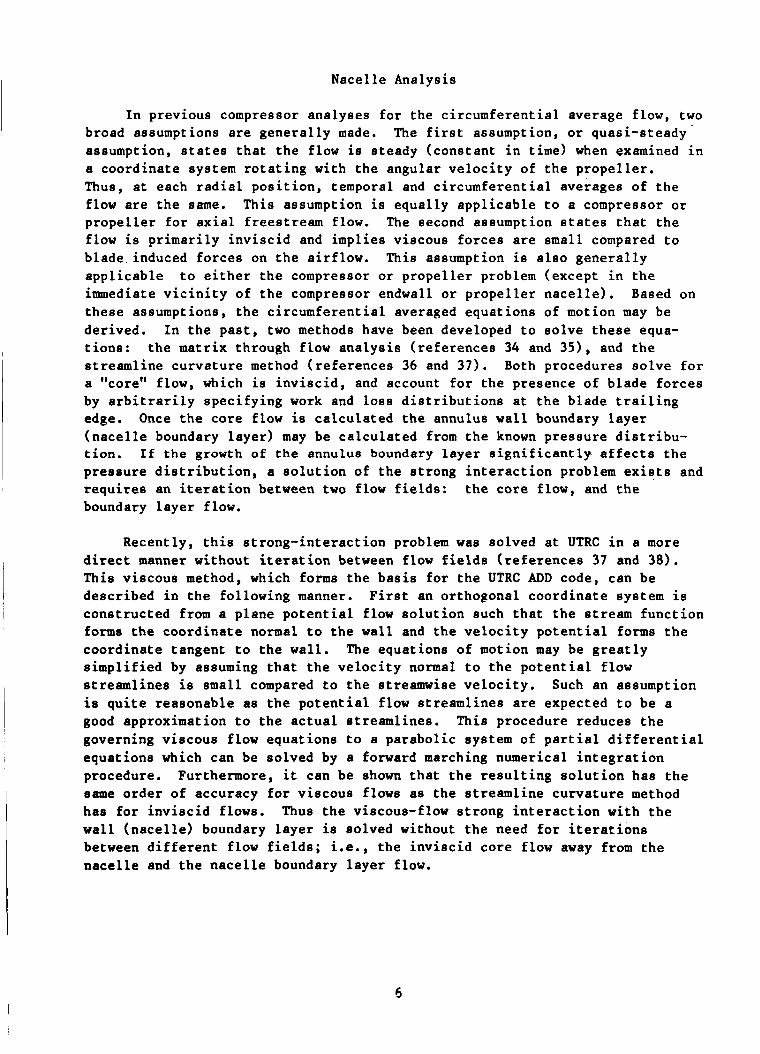
In previous compressor analyses for the circumferential average flow, two broad assumptions are generally made. The first assumption, or quasi-steady assumption, states that the flow is steady (constant in time) when examined in a coordinate system rotating with the angular velocity of the propeller. Thus, at each radial position, temporal and circumferential averages of the flow are the same. propeller for axial freestream flow. The second assumption states that the flow is primarily inviscid and implies viscous forces are small compared to blade induced forces on the airflow. applicable to either the compressor or propeller problem (except in the immediate vicinity of the compressor endwall or propeller nacelle). these assumptions, the circumferential averaged equations of motion may be derived. tions: streamline curvature method (references 36 and 37) . Both procedures solve for a "core" flow, which is inviscid, and account for the presence of blade forces by arbitrarily specifying work and loss distributions at the blade trailing edge. Once the core flow is calculated the annulus wall boundary layer (nacelle boundary layer) may be calculated from the known pressure distribution. If the growth of the annulus boundary layer significantly affects the pressure distribution, a solution of the strong interaction problem exists and requires an iteration between two flow fields: the core flow, and the boundary layer flow.

This assumption is equally applicable to a compressor or

This assumption is also generally

Based on

In the past, two methods have been developed to solve these equa- the matrix through flow analysis (references 34 and 351, and the

Recently, this strong-interaction problem was solved at UTRC in a more direct manner without iteration between flow fields (references 37 and 38). This viscous method, which forms the basis for the UTRC ADD code, can be described in the following manner. First an orthogonal coordinate system is constructed from a plane potential flow solution such that the stream function forms the coordinate normal to the wall and the velocity potential forms the coordinate tangent to the wall. simplified by assuming that the velocity normal to the potential flow streamlines is small compared to the streamwise velocity. is quite reasonable as the potential flow streamlines are expected to be a good approximation to the actual streamlines. This procedure reduces the governing viscous flow equations to a parabolic system of partial differential equations which can be solved by a forward marching numerical integration procedure. Furthermore, it can be shown that the resulting solution has the same order of accuracy for viscous flows as the streamline curvature method has for inviscid flows. Thus the viscous-flow strong interaction with the wall (nacelle) boundary layer is solved without the need for iterations between different flow fields; i.e., the inviscid core flow away from the nacelle and the nacelle boundary layer flow.

The equations of motion may be greatly

Such an assumption

6

Combined Analysis

The approach taken to create the combined propeller-nacelle analysis was to use a modified version of the original UTRC ADD code which includes the required refinements necessary for the nacelle-propeller problem. The calculation of the blade forces was handled by creating as a portion of the combined analysis an expanded propeller lifting line solution procedure based on existing UTC propeller and helicopter performance analyses. This combined analysis consists of two portions (propeller and nacelle) which compute the combined propeller-nacelle performance by interfacing the required transfer of internal data (flow field properties, wake geometry displacements, and blade forces) which will influence the respective solution procedures from the two different portions of the analysis. This procedure allows the combined analysis to have the ability to also calculate isolated propeller or isolated nacelle performance for comparisons with the combined propeller-nacelle configuration performance predictions. A simplified diagram of the program task structure of the combined analysis is presented in figure 3. The details of the technical approach of each portion of the analysis and the coupling procedure of the combined analysis are presented in the following sections.

7

TECHNICAL APPROACH - PROPELLER

Overview

In the following sections, a method of analysis for the predictions of the integrated and local spanwise blade air loading for the high speed propeller is presented. The analysis presented for the high speed propeller portion of the combined propeller-nacelle code is a logical extension of the development of the Prescribed Wake Method of Landgrebe (reference 26) for hovering rotors which was modified and applied to statically thrusting propellers by Landgrebe and then Ladden (reference 1 7 ) . Although this analysis is directed towards the high speed propeller flight regime, no restric- tions have been made in the assumptions which would limit it to only high speed flight. line theory, and incorporates a wake model consisting of a finite number of trailing vortex filaments. The trajectories and positioning of these filaments must be prescribed. prescribed wake models used for hovering rotors (similar representations are used for propellers). tion is solved utilizing the Kutta-Joukowski and Biot-Savart relations, and the airfoil lift properties. tribution and the corresponding induced velocities. The blade element velocity diagram is then constructed, and with the use of two-dimensional airfoil data corrected for three-dimensional tip effects, the airloading distribution (lift and drag) is obtained. The total thrust and power are then established through spanwise integration.

Briefly the Prescribed Wake method is derived utilizing lifting

Figure 4 is an illustration of two types of

Once the position of the wake is fixed, a matrix solu-

This solution yields the blade circulation dis-

The use of the propeller analysis in conjunction with the nacelle code is handled in a coupled manner, whereby the nacelle's influence on the propeller is incorporated through modifications to the noninduced inflow at the propeller disk and to the wake model. The theory of the analysis as outlined in the following sections does not make direct reference to the nacelle's influence on the velocites. It is thus understood that the noninduced velocity terms include the nacelle's influence in the following propeller related sections.

9

Coordinate Systems

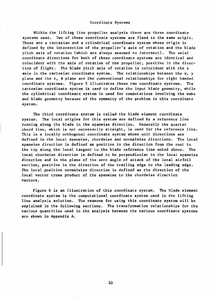
Within the lifting line propeller analysis there are three coordinate systems used. Two of these coordinate systems are fixed to the same origin. These are a Cartesian and a cylindrical coordinate system whose oriein is defined by the intersection of the propeller's axis of rotation and the blade pitch axis of rotation (which are always assumed to intersect). coordinate directions for both of these coordinate systems are identical and coincident with the axis of rotation of the propeller, positive in the direction of flight. The blade pitch axis of rotation is coincident with the x axis in the Cartesian coordinate system. The relationships between the x, y plane and the r, 0 plane are the conventional relationships for right handed coordinate systems. Figure 5 illustrates these two coordinate systems. The Cartesian coordinate system is used to define the input blade geometry, while the cylindrical coordinate system is used for computations involving the wake and blade geometry because of the symmetry of the problem in this coordinate system.

The axial

The third coordinate system is called the blade element coordinate system. running along the blade in the spanwise direction. chord line, which is not necessarily straight, is used for the reference line. This is a locally orthogonal coordinate system whose unit directions are defined in the local spanwise, chordwise and normalwise directions. The local spanwise direction is defined as positive in the direction from the root to the tip along the local tangent to the blade reference line noted above. The local chordwise direction is defined to be perpendicular to the local spanwise direction and in the plane of the zero angle of attack of the local airfoil section, positive in the direction of the trailing edge to the leading edge. The local positive normalwise direction is defined as the direction of the local vector cross product of the spanwise to the chordwise direction vectors.

The local origins for this system are defined by a reference line Generally the quarter

Figure 6 is an illustration of this coordinate system. The blade element coordinate system is the computational coordinate system used in the lifting line analysis solution. explained in the following sections. The transformation relationships for the various quantities used in the analysis between the various coordinate systems are shown in Appendix A.

The reasons for using this coordinate system will be

10 '

Propeller Lifting Line Theory

The concept of a prescribed wake lifting line theory applied to propellers consists essentially of assuming that the blade of each propeller can be represented by a segmented bound vortex lifting line located along the propeller blade quarter chord line with a spanwise varying concentrated circulation strength which at each segment is proportional to the local blade lift (Kutta-Joukowski Law). discrete trailing vortices whose circulation strength is a function of radial variations in the blade loading (lift) distribution. A finite length wake is used which is of sufficient length to approximately model an infinite length wake. Figure 7 is an illustration of this modeling procedure. There are N segments modeling the blade which can be arbitrary in length. strength of the bound vortex Over each segment is assumed to be constant, and the values of the strength are determined by the aerodynamics of the problem which are discussed in the next section. single propeller under steady axial flight conditions is time independent, there is no azimuthal variation in blade loading for the single propeller configuration. trailing segmented vortex filaments shed from the junction points of the blade bound vortex segments whose circulation strength is constant over the complete length of the filament and equal to the difference in the circulation strengths of the adjacent bound vortex segments. Figure 7 also illustrates this feature. The trailing filament segmentation is defined by a specified azimuthal step size (A$), each segment modeled by a straight line vortex segment. The location of the trailing wake segment end points are prescribed by using various types of wake models.

The wake is assumed to be modeled by a system of

The circulation

Because the flow field sensed by the

The wake shed by the blade can be modeled by a series of

The influence of the bound and trailing vortex elements at any field point is computed by using the Biot-Savart Law for finite length, straight line segments of constant strength (reference 8) a8 shown in Appendix B. this analysis the calculation is done in the cylindrical coordinate system and then transformed to the blade element coordinate system. The induced velocity vector, FTR,- at a local blade element in the local. blade element coordinate system due to any trai€ing segment can be written as

In

where the subscripts 8 , c and n denote the spanwise, chordwise and normalwise directions respectively. Any one of these induced velocity components can be expressed as the sum of the products of the trailing segment chculation strength and the appropriate component of the geometric inf 1ue;ice coefficient computed from the Biot-Savart Law as noted in Appendix B. For example the normalwise induced velocity from the lth segment of the kth filament of the mth blade is

11

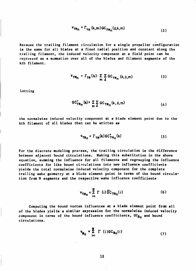
Because the trailing filament circulation for a single propeller configuration is the same for all blades at a fixed radial position and constant along the trailing filament, the induced velocity component at a field point can be ~xpressed as a summation over all of the blades and filament segments of the kth filament.

Letting

the normalwise induced velocity component at a blade element point due to the kth filament of all blades then can be written as

For the discrete modeling process, the trailing circulation is the difference between adjacent bound circulations. Making this substitution in the above equation, sumning the influence for all filaments and regrouping the influence coefficients for like bound circulations into new influence coefficients yields the total normalwise induced velocity component for the complete trailing wake geometry at a bla'de element point in terms of the bound circulation fran N segments and the respective wake influence coefficients

Computing the bound vortex influencer at a blade element point frau all of the blades yields a similar expression for the normalwire induced velocity component in terms of the bound influence coefficients, G C B ~ and bound circulations.

12

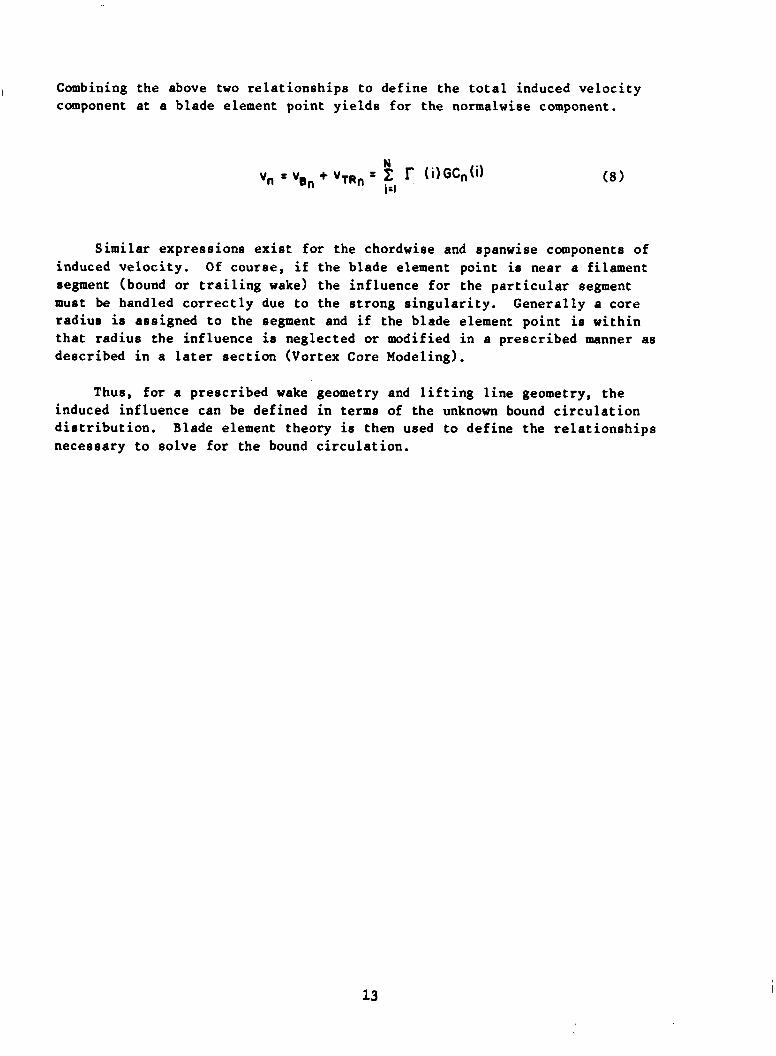
1 Combining the above two relationships to define the total induced velocity component at a blade element point yields for the normalwise component.

Similar expressions exist for the chordwise and spanwise components of induced velocity. Of course, if the blade element point is near a filament segment (bound or trailing wake) the influence for the particular segment must be handled correctly due to the strong singularity. Generally a core radius is assigned to the segment and if the blade element point is within that radius the influence is neglected or modified in a prescribed manner as described in a later section (Vortex Core Modeling).

Thus, for a prescribed wake geometry and lifting line geometry, the induced influence can be defined in terms of the unknown bound circulation distribution. necessary to solve for the bound circulation.

Blade element theory is then used to define the relationships

13

Blade Element Aerodynamics

The modeling of the propeller blade by the Lifting line approach defines the inflow and the effective angle of attack at each blade segment in the aerodynamic model. Tabulated airfoil data is used to relate the effective angle of attack at each blade segment to the local lift and drag characteristics. Also, the use of tabulated airfoil data, acquired from two-dimensional airfoil tests, inherently accounts for the chordwise vorticity distribution (related to chordwise pressure distribution) and the Kutta condition. This permits the blade segments to be represented by bound vortex segments which have a circulation strength representative of the integrated chordwise vorticity distribution. For a lifting line model, the unknown quantity is then the spanwise bound circulation distribution which is related to the lift distribution through the Kutta-Joukowski relationship as will be described.

In figure 8 the relationships between the relative velocity vectors and the geometric quantities in the local blade element coordinate system are illustrated. It is assumed that the propeller is operating in steady axial flight. This blade element coordinate system is the computational coordinate system and the solution for the blade forces is done in this coordinate system. One reason to use this coordinate system is that the angle of attack is small and the chordwise velocity is the dominant velocity term in this coordinate system. This makes the solution numerically easier to obtain in the blade element coordinate system. Another reason to use this coordinate system is that the resolution of the blade geometry quantities and velocities into this coordinate system implicity handles the concept of yaw or skewed flow aerodynamics. The concept of skewed flow aerodynamics (in the two- dimensional sense) basically states that the pressure force on an airfoil section is independent of the spanwise flow velocity component, and thus a function of only the velocity components in the plane normal to the local chordwise direction (reference for local blade element coordinate system). In the relationships to follow, the aerodynamic quantities used are assumed to be those which correspond to the local blade element coordinate system. Each blade element section is treated as a two-dimensional section with the influence of the other sections transmitted through the induced flowfield.

Linear Aerodynamics

The aerodynamic relationships for the blade forces include nonlinear behavior with certain quantities. The nonlinear solution is obtained by using the linearized solution with the appropriate nonlinear iteration techniques as will be described in the next section.

In the blade element coordinate system the local velocity vector diagrams appear similar to the equivalent velocity vector diagrams of a statically thrusting propeller. independent of time. For this reason, the linearization procedure and

In this coordinate system the solution on the blades is

14

solution techniques are best performed in the local blade element coordinate system. The linearizations follow directly from those presented in reference 17 for the statically thrusting propeller.

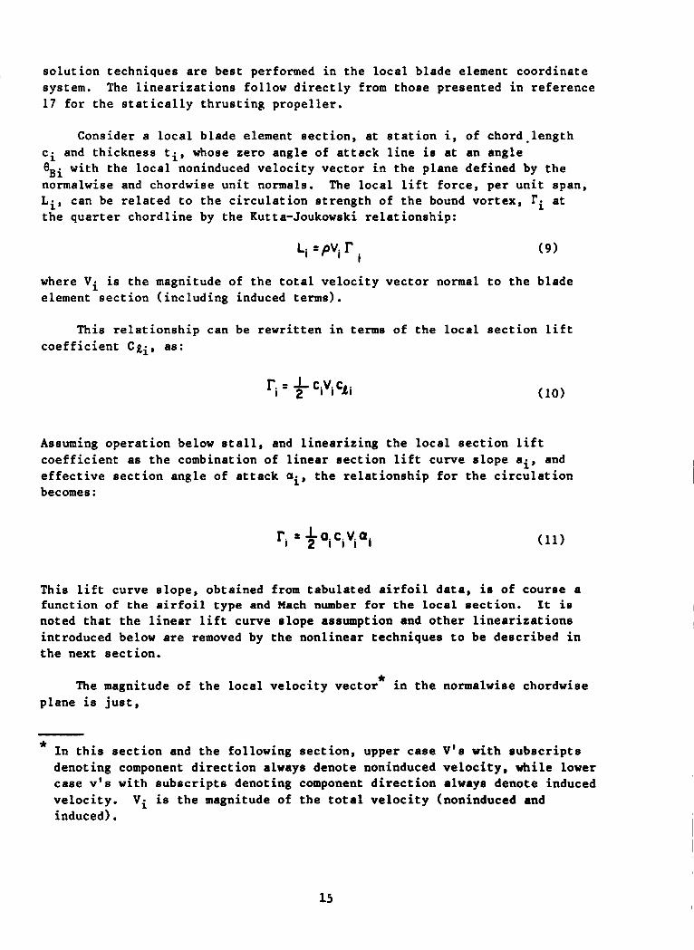
Consider a local blade element section, at station is of chord-length ci and thickness ti, whose zero angle of attack line is at an angle eBi with the local noninduced velocity vector in the plane defined by the normalwise and chordwise unit normals. The local lift force, per unit span, Lis can be related to the circulation strength of the bound vortex, ri at the quarter chordline by the Kutta-Joukowski relationship:

L~ =pi r i

( 9 )

where Vi is the magnitude of the total velocity vector normal to the blade element section (including induced terms).

This relationship can be rewritten in terms of the local section lift coefficient Cg; , as :

ri = + civicAi (10)

Assuming operation below stall, and linearizing the local section lift coefficient as the combination of linear section lift curve slope ai, and effective section angle of attack ai, the relationship for the circulation becomes :

ri = +aicivia, (11)

This lift curve slope, obtained from tabulated airfoil data, is of course a function of the airfoil type and Mach number for the local section. It is noted that the linear lift curve slope assumption and other linearizations introduced below are removed by the nonlinear techniques to be described in the next section.

* The magnitude of the local velocity vector in the normalwise chordwise

plane is just,

* In this section and the following section, upper case V ' s with subscripts denoting component direction always denote noninduced velocity, while lower case v's with subscripts denoting component direction always denote induced velocity. induced).

Vi is the magnitude of the total velocity (noninduced and

15

I .

vi .[(VCi+VCi)2 + (Vni+ vnif]”2 (12)

Assuming that in the blade element plane the induced and normal velocities are small compared with the chordwise noninduced velocity yields the following approximation for the section circulation.

From figure 7 it can be seen that the blade element section angle of attack is just:

If the chordwise induced velocity is neglected, the section angle of attack is assumed to be small, and the normal velocity is also small with respect to the chordwise value, the blade circulation is further approximated as

where

ri = I C,aivcI (e,i + vni ) VCi

(15)

The normalwise induced velocity, vni is a function of the combined wake geometry from all blades and the blade circulations, where the normalwise geometric influence coefficients are computed using the Biot-Savart Law (see section entitled: Lifting Line Theory). Then from equation (81, the blade circulation of section i can be written as:

This relationship is valid under the above assumptions for each blade element section, thus a system of simultaneous linear equations in terms of the unknown blade circulations for each section can be written as a matrix equation in the form:

16

I and the solution for the circulations can be obtained directly using standard solution techniques, either iterative or direct techniques. Because the number of unknowns is relatively small, the analysis uses a Gauss-Jordan reduction technique.

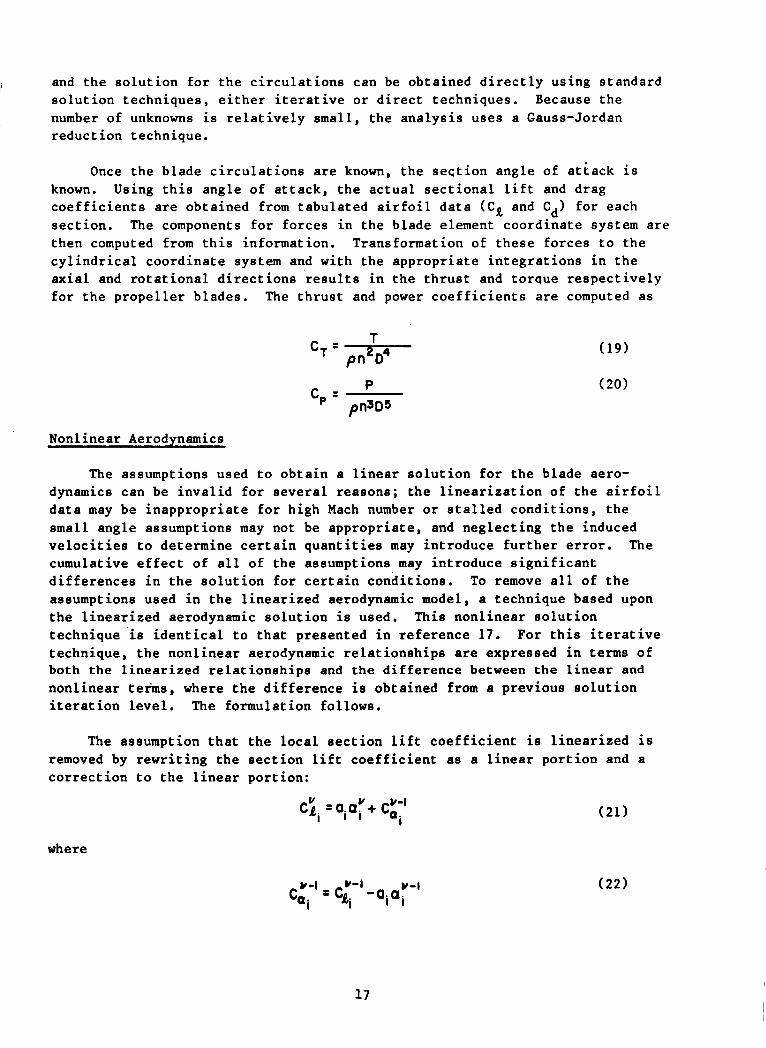
Once the blade circulations are known, the section angle of attack is known. Using this angle of attack, the actual sectional lift and drag coefficients are obtained from tabulated airfoil data (C, and Cd) for each section. The components for forces in the blade element coordinate system are then computed from this information. Transformation of these forces to the cylindrical coordinate system and with the appropriate integrations in the axial and rotational directions results in the thrust and torque respectively for the propeller blades. The thrust and power coefficients are computed as

I ' T = pn2D4 (19)

Nonlinear Aerodynamics

The assumptions used to obtain a linear solution for the blade aerodynamics can be invalid for several reasons; the linearization of the airfoil data may be inappropriate for high Mach number or stalled conditions, the small angle assumptions may not be appropriate, and neglecting the induced velocities to determine certain quantities may introduce further error. The cumulative effect of all of the assumptions may introduce significant differences in the solution for certain conditions. assumptions used in the linearized aerodynamic model, a technique based upon the linearized aerodynamic solution is used. technique 'is identical to that presented in reference 17. technique, the nonlinear aerodynamic relationships are expressed in terms of both the linearized relationships and the difference between the linear and nonlinear tefms, where the difference is obtained from a previous solution iteration level. The formulation follows.

To remove all of the

This nonlinear solution For this iterative

The assumption that the local section lift coefficient is linearized is removed by rewriting the section lift coefficient as a linear portion and a correction to the linear portion:

V u r-l I i

CQ. = oiai + c,

where

(21)

17

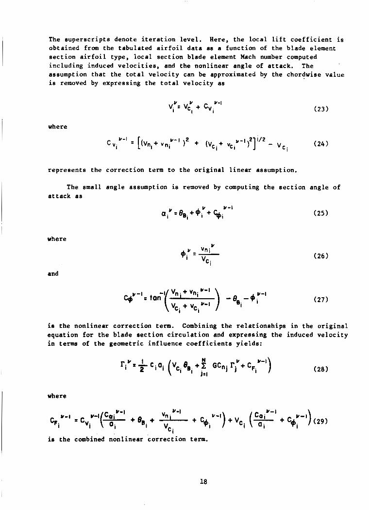
The superscripts denote iteration level. obtained from the tabulated airfoil data as a function of the blade element section airfoil type, local section blade element Mach number computed including induced velocities, and the nonlinear angle of attack. The assumption that the total velocity can be approximated by the chordwise value is removed by expressing the total velocity as

Here, the local lift coefficient is

V U If-l vi = vc. + C". I I

where

(23)

represents the correction term to the original linear assumption.

The small angle assumption is removed by computing the section angle of attack as

V a i y = 8 B i + + i + (25 )

where

and

(26 )

is the nonlinear correction term. Combining the relationships in the original equation for the blade section circulation and expressing the induced velocity in terms of the geometric influence coefficients yields:

N V

i.1 i rip- I ciai (Vci6,++z G C n j r j +C, -2 (28)

where

is the combined nonlinear correction term.

18

I If the combined nonlinear correction term, C F ~ , linearized equation for the blade circulation r

is set to zero, the sults. If the above e uat ion

is rewritten in matrix form in terms of the unknown blade circulations, a system of simultaneous linear equations results where the correction term is lagged in iteration level.

This system of equations can be solved by direct or indirect methods for each iteration level where the previous solution is used to obtain the latest nonlinear correction terms for each iteration. The initial correction terms are obtained from the initital linearized solution. In the current analysis the Gauss-Jordan reduction technique is used to obtain the solution at each iteration level.

The resulting local blade forces in the chordwise and normalwise directions are obtained in the same manner as is done for the linearized solution, and the resultant integrated forces are obtained.

Skewed Flow Drag Model

As noted in an earlier section (Blade Element Aerodynamics) , the calculation of the blade forces in the blade element coordinate system removes the necessity of considering skewed flow in an explicit manner in the aerodynamic relationships for the pressure lift and pressure drag forces. However, the drag coefficient data available for airfoils generally does not distinguish between the pressure drag and friction drag components. Since the friction drag should be dependent on the total velocity, a skewed flow drag model is formulated below using the tabulated drag coefficient data. This model attempts to include the additional component of skin friction drag neglected by the blade element aerodynamic model described in the previous sect ion.

Figure 9 is a vector diagram of the drag force and components of the drag force at a local blade element station for a condition with a velocity component in the spanwise direction. From this diagram it can be seen that the total drag force, D (per unit area), has been broken into two portions, a

The pressure pressure drag force, drag acts only in the direction of the flaw in the plane defined by the chordwise and normalwise directions, while the friction drag is assumed to act in the direction of the total velocity. the spanwise velocity component, and computing the drag force, with the

and a skin friction drag force, Dfr. DPt.,

The conventional method of neglecting

! 19

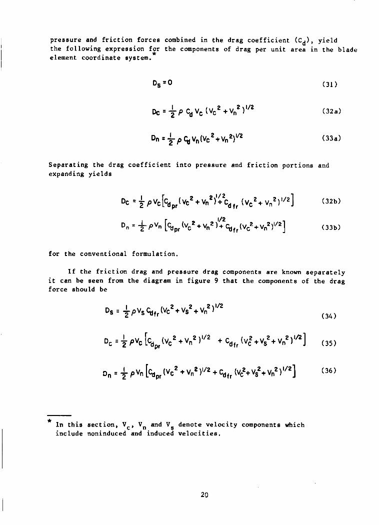
pressure and friction forces combined in the drag coefficient tcd), yield the following expression for the components of drag per unit area in the blade element coordinate system.

*

Separating the drag coe expanding yields

icient into pressure and fr,:tion portions and

for the conventional formulation.

If the friction drag and pressure drag components are known separately it can be seen from the diagram in figure 9 that the components of the drag force should be

* In this section, Vc, Vn and V, denote velocity components which include noninduced and induced velocities.

20

From these relationships it can be seen that for large spanwise velocities, the drag force components can be significantly different as compared with the conventional formulation. The above formulation has been incorporated into the analysis as an optional feature by assuming that the skin friction drag coefficient is approximately represented by the drag coefficient of the section at zero angle of attack, cdos and thus the pressure drag coefficient is just the difference between the total drag coefficient and cdo.

Tip Relief Models

The high speed propeller tip experiences high subsonic and transonic flow conditions at normal design operating conditions. These flow conditions, coupled with the high degree of three-dimensionality of the problem and the use of two-dimensional airfoil characteristics, make the application of the lifting line model inappropriate without some type of tip relief scaling procedures applied to the airfoil characteristics in the tip region. Two such models have been incorporated into the propeller analysis. The first is a model based on unswept fixed wing theory. conical flow theory applied to swept wings.

The second is a model based on

Evvard T~J Relief Model ---- - - - - - - For flow conditions where the tip Mach number is greater than one and the

forward speed Mach number less than one, it is necessary to correct the pressure forces in the propeller tip Mach cone region. Figure 10 illustrates the region on the blade under consideration. In reference 41, charts for a scaling factor which is a function of the ratio of blade chord to blade radius, radial location on the blade, and tip Mach number are presented which can be used to correct the epanwise variation of lift and drag due to lift. These charts where derived from the results for fixed wings presented by E w a r d in reference 42. included as an option to the aerodynamic model. It should be noted that this model was developed from fixed wing results for application to conventional propeller blades without sweep, thus the application to swept blades is ques- t ionable.

In the current analysis this scaling factor is

The application of the scaling function to the lift and drag due to lift is done by determining the spanwise location where the tip Mach cone inter- sects the blade at a specified fraction of the chord from the leading edge

21

(generally the trailing edge is used). to the blade tip are modified by the appropriate scaling value if the local free stream Mach number is greater than or equal to one. are tabulated and are an integral part of the analysis. Both the spatial location used to define the point for the definition of the tip Mach cone location and the fraction of the chord for the intersection location can be varied in the analysis. values is also available in the analysis and it gives slightly different values than the original tables.

All blade stations from this location

These scaling values

An analytical description for the tip relief scaling

Conical Flow Theory Tin Relief Model --------- ------ Generally, high speed propeller designs require significant blade sweep,

therefore the application of the tip relief model based on Evvard's model may not be appropriate for these applications. Conical flow theory for thin swept wings with sweep can be used to provide a tip relief model for application to the swept propeller blade. The model as developed for application to swept propeller blades in based on a tapered, swept, fixed wing configuration which assumes that the wing leading edge is linear and subsonic and that the wing trailing edge is linear and supersonic for a constant supersonic freestream Mach number distribution. Furthermore, the span of the wing is assumed to be of s u f f i c i e n t length to avoid overlap of the t i p Mach cones on the wing surface and the wing tip is squared off. These assumptions result in the existence of two regions on the surface of the wing for which a scaling function based on the ratio of the three-dimensional section lift to the two- dimensional section lift can be obtained. The regions on the surface of the wing are depicted in figure 11 which also defines the wing planform shape and the coordinate system used in the formulation. On the surface of the wing in region I along any section chordline of length c, the chordwise pressure distribution based on conical flow theory (reference 4 3 ) for a subsonic leading edge in the above configuration can be integrated along the chordline to obtain the appropriate section lift in the region,

where B = (M2-1)'/2, m B cot ALE, k (1-m2)'12

and E'(k) is the complete Elliptic Integral of the second kind of modulus k.

22

On the surface of the wing in region I1 the chordwise integration of the pressure distribution, approximately a constant deficit along the chordline from the value at the edge of this region, is performed to obtain the appropriate section lift in the region.

1 dx 1

J2(1+m>(i-y/~> - c =

(39 > 4ma (x,-x.,> r x., 1 1

These two section lifts are combined to obtain the total section two-dimensional section lift for the same freestream Mach number

40 = - CL2D B

lift. The is known.

(40 >

The scaling function is then just the ratio of the three-dimensional to the two-dimensional section lift.

This scaling function can then be applied to the supersonic region of the propeller tip by assuming that the length of this region is equivalent to the semi-span of a supersonic wing with a freestream Mach number equal to the propeller tip Mach number. This scaling function is included as an option in the analysis. Since the model as derived is based on a constant Mach number and the propeller blade senses a radially varying distribution, an approximation for this effect can be incorporated by scaling the relationship of equation (40) by the ratio defined below based on Prandtl-Glauert compressible scaling rule.

(42 >

This feature is also included in the analysis as an option available to the user.

23

A i r f o i l Data

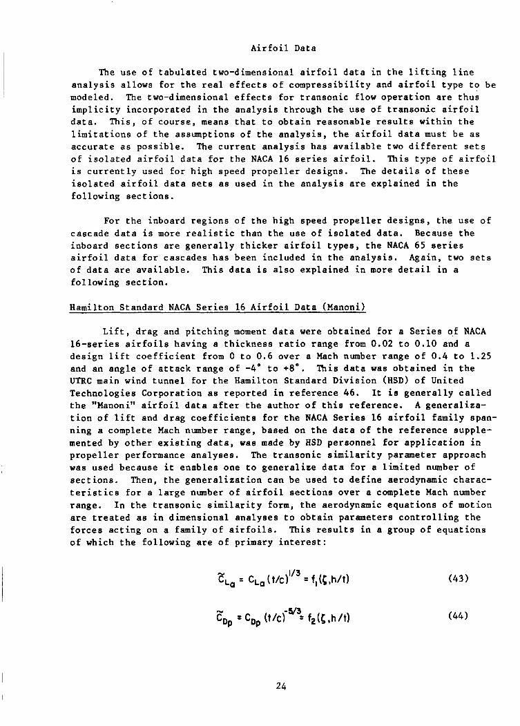
The use of t abu la t ed two-dimensional a i r f o i l d a t a i n t h e l i f t i n g l i n e a n a l y s i s a l lows f o r t h e r e a l e f f e c t s o f c o m p r e s s i b i l i t y and a i r f o i l type t o be modeled. The two-dimensional e f f e c t s f o r t r a n s o n i c flow o p e r a t i o n are t h u s i m p l i c i t y incorpora ted i n t h e a n a l y s i s through t h e use of t r a n s o n i c a i r f o i l d a t a . This, of cour se , means t h a t t o o b t a i n reasonable r e s u l t s w i th in t h e l i m i t a t i o n s of t h e assumptions of t h e a n a l y s i s , t h e a i r f o i l d a t a must be a s a c c u r a t e a s poss ib l e . o f i s o l a t e d a i r f o i l d a t a f o r t h e NACA 16 s e r i e s a i r f o i l . This type of a i r f o i l i s c u r r e n t l y used f o r high speed p r o p e l l e r des igns . The d e t a i l s o f t h e s e i s o l a t e d a i r f o i l d a t a se ts as used i n t h e a n a l y s i s a r e explained i n t h e fo l lowing s e c t i o n s .

The c u r r e n t a n a l y s i s has a v a i l a b l e two d i f f e r e n t s e t s

For t h e inboard r eg ions of t h e high speed p r o p e l l e r des igns , t h e use o f cascade d a t a i s more r e a l i s t i c than t h e use of i s o l a t e d d a t a . Because t h e inboard s e c t i o n s a r e g e n e r a l l y t h i c k e r a i r f o i l t y p e s , t h e NACA 65 s e r i e s a i r f o i l d a t a f o r cascades h a s been included i n t h e a n a l y s i s . Again, two s e t s o f d a t a are a v a i l a b l e . This d a t a i s a l s o expla ined i n more d e t a i l i n a fo l lowing s e c t i o n .

Hamilton S tandard NACA S e r i e s 16 A i r f o i l Data (Manoni)

L i f t , d rag and p i t c h i n g moment d a t a were obta ined f o r a S e r i e s of NACA 16 - se r i e s a i r f o i l s having a t h i c k n e s s r a t i o range from 0.02 t o 0.10 and a d e s i g n l i f t c o e f f i c i e n t from 0 t o 0.6 over a Mach number range o f 0 . 4 t o 1.25 and an ang le o f a t t a c k range of -4' t o +a'. UTRC main wind tunne l f o r t h e Hamilton Standard Div i s ion (HSD) of United Technologies Corpora t ion a s r epor t ed i n r e f e r e n c e 46. t h e "Manoni" a i r f o i l d a t a a f t e r t h e au tho r o f t h i s r e fe rence . t i o n o f l i f t and d rag c o e f f i c i e n t s f o r t h e NACA S e r i e s 16 a i r f o i l fami ly span- n ing a complete Mach number range , based on t h e d a t a o f t h e r e f e r e n c e supple- mented by o t h e r e x i s t i n g d a t a , was made by HSD personnel f o r a p p l i c a t i o n i n p r o p e l l e r performance ana lyses . The t r a n s o n i c s i m i l a r i t y parameter approach was used because i t enab le s one t o g e n e r a l i z e d a t a f o r a l i m i t e d number of s e c t i o n s . Then, t h e g e n e r a l i z a t i o n can be used t o d e f i n e aerodynamic charac- t e r i s t i c s f o r a l a r g e number of a i r f o i l s e c t i o n s over a complete Mach number range. I n t h e t r a n s o n i c s i m i l a r i t y form, t h e aerodynamic equa t ions of motion a r e t r e a t e d a s i n dimensional ana lyses t o o b t a i n parameters c o n t r o l l i n g t h e f o r c e s a c t i n g on a family o f a i r f o i l s . o f which t h e fo l lowing a r e of primary i n t e r e s t :

This d a t a was obta ined i n t h e

It i s g e n e r a l l y c a l l e d A gene ra l i za -

This r e s u l t s i n a group o f equa t ions

24

(45 1

(46

The above symbols a r e def ined i n t h e L i s t of Symbols.

In o r d e r t o make t h e g e n e r a l i z a t i o n a p p l i c a b l e t o h ighe r t h i c k n e s s r a t i o s , a d d i t i o n a l ad jus tments had t o be included. This r e s u l t i n g gene ra l i za - t i o n spans t h e following ranges :

Mach Number 0 .3 t o 1.25

Thickness Rat i o 0.02 t o 0.40 Design L i f t C o e f f i c i e n t

Angle of Attack -4" t o +8"

0 t o 0.7

and has been implemented i n t o t h i s p rope l l e r -nace l l e performance a n a l y s i s .

Publ i shed NACA S e r i e s 16 A i r f o i l Data (NACA)

In r e f e r e n c e 47 two-dimensional a i r f o i l d a t a f o r NACA S e r i e s 16 a i r f o i l s e c t i o n s a r e p re sen ted . The d a t a was developed from a compi la t ion o f a l l t h e d a t a a v a i l a b l e up t o t h e e a r l y 1950's and t h e e f f o r t was somewhat handicapped by t h e l a c k o f d a t a throughout t h e t r a n s o n i c Mach number reg ion . cover a range o f t h i c k n e s s r a t i o s of 4 t o 2 1 percent and des ign l i f t c o e f f i - c i e n t o f 0 t o 0.7 . c o e f f i c i e n t , CL, as a func t ion o f f r ees t r eam Mach number and a i r f o i l des ign l i f t c o e f f i c i e n t . personnel spanning t h e fo l lowing ranges:

The d a t a

The l i f t d a t a a r e presented i n t h e form of curves of l i f t

Data from t h e r e f e r e n c e was p a r t i a l l y computerized by HSD

Mach Number 0.3 t o 1.15 Angle of At tack -6" t o +12' Thickness Ra t io 0.03 t o 0.09 Design L i f t C o e f f i c i e n t 0 t o 0.2

The d a t a was e x t r a p o l a t e d t o o b t a i n 0.03 t h i c k n e s s r a t i o . The t h i c k n e s s r a t i o and des ign l i f t c o e f f i c i e n t ranges can be extended from t h e d a t a provided i n t h e r e fe rence . This d a t a i s g e n e r a l l y l abe led t h e "NACA" a i r f o i l d a t a .

Cascade A i r f o i l Data (NASA SP-36)

S ince t h e inboard s e c t i o n s o f a h igh speed p r o p e l l e r d e s i g n can approach gap t o chord r a t i o s which r e p r e s e n t cascade a i r f o i l c o n d i t i o n s , a set o f cascade a i r f o i l d a t a c o r r e l a t i o n s has been incorpora ted i n t h e a n a l y s i s f o r t y p i c a l h igh speed p r o p e l l e r des ign requi rements . based on t h e NACA 65 s e r i e s A = 1 meanline. This cascade c o r r e l a t i o n is v a l i d

The cascade c o r r e l a t i o n i s

25

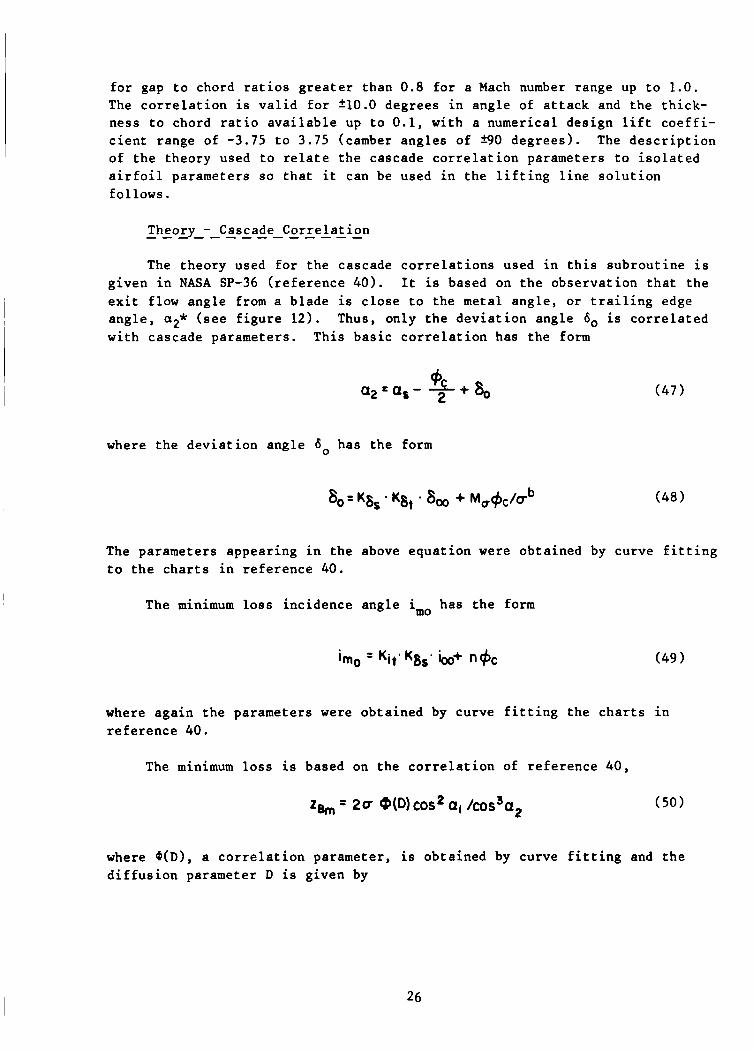
f o r gap t o chord r a t i o s g r e a t e r than 0.8 f o r a Mach number range up t o 1 .0 . The c o r r e l a t i o n i s v a l i d f o r 210.0 degrees i n angle of a t t a c k and the th ick- ness t o chord r a t i o a v a i l a b l e up t o 0 .1 , with a numerical design l i f t c o e f f i - c i e n t range of -3.75 t o 3 . 7 5 (camber angles of S O degrees) . The d e s c r i p t i o n of t he theory used t o r e l a t e t he cascade c o r r e l a t i o n parameters t o i s o l a t e d a i r f o i l parameters so t h a t it can be used i n the l i f t i n g l i n e s o l u t i o n fo l lows .

The theory used f o r the cascade c o r r e l a t i o n s used i n t h i s subrout ine i s g iven i n NASA SP-36 ( r e fe rence 4 0 ) . It is based on t h e observa t ion t h a t t he e x i t flow angle from a blade i s c l o s e t o the metal angle , o r t r a i l i n g edge ang le , a2* ( s e e f i g u r e 12) . Thus, only t h e d e v i a t i o n angle 6, is c o r r e l a t e d with cascade parameters. This bas i c c o r r e l a t i o n has the form

where the d e v i a t i o n angle 60 has the form

The parameters appearing i n the above equat ion were obtained by curve f i t t i n g t o t h e c h a r t s i n r e fe rence 4 0 .

The minimum l o s s inc idence angle imo has the form

where aga in the parameters were obtained by curve f i t t i n g the c h a r t s i n r e fe rence 4 0 .

The minimum l o s s i s based on the c o r r e l a t i o n of r e fe rence 4 0 ,

where @(D), a c o r r e l a t i o n parameter, is obtained by curve f i t t i n g and t h e d i f f u s i o n parameter D i s given by

26

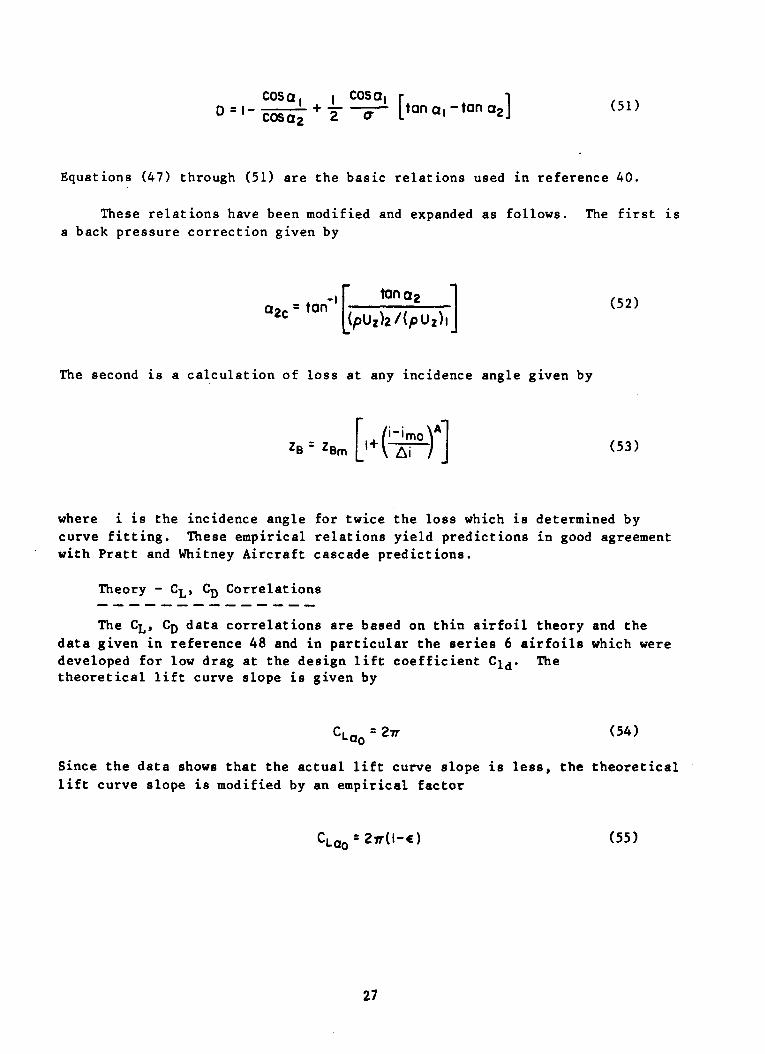
Equat ions (47) through (51) a r e t h e b a s i c r e l a t i o n s used i n r e f e r e n c e 40.

These r e l a t i o n s have been modified and expanded a s fo l lows . The f i r s t i s a back p res su re c o r r e c t i o n g iven by

The second i s a c a l c u l a t i o n of l o s s a t any inc idence angle g iven by

where i i s t h e inc idence angle f o r twice t h e l o s s which i s determined by curve f i t t i n g . wi th P r a t t and Whitney A i r c r a f t cascade p r e d i c t i o n s .

These empi r i ca l r e l a t i o n s y i e l d p r e d i c t i o n s i n good agreement

Theory - CL, CD C o r r e l a t i o n s

The CL, CD d a t a c o r r e l a t i o n s a r e based on t h i n a i r f o i l theory and t h e

--------------

d a t a g iven i n r e f e r e n c e 48 and i n p a r t i c u l a r t h e series 6 a i r f o i l s which were developed f o r low d rag a t t h e des ign l i f t c o e f f i c i e n t C l d . t h e o r e t i c a l l i f t curve s lope i s g iven by

The

Since t h e d a t a shows t h a t t h e a c t u a l l i f t curve s lope i s less, t h e t h e o r e t i c a l l i f t cu rve s l o p e i s modif ied by an empi r i ca l f a c t o r

27

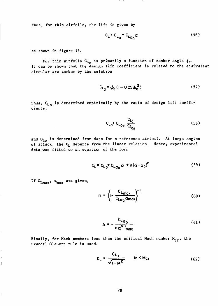
Thus, for thin airfoils, the lift is given by

c,= CL0+ c, Q 00

as shown in figure 13.

(56)

For thin airfoils C L ~ is primarily a function of camber angle +c. It can be shown that the design lift coefficient is related to the equivalent circular arc camber by the relation

Thus, C L ~ is determined empirically by the ratio of design lift coefficients,

and C L ~ is determined, from data for a reference airfoil. of attack, the CL departs from the linear relation. Hence, experimental data was fitted to an equation of the form

At large angles

If CLmax, amax are given,

Finally, fo r Mach numbers less than the critical Mach number Mcr, the Prandtl Glauert rule is used.

28

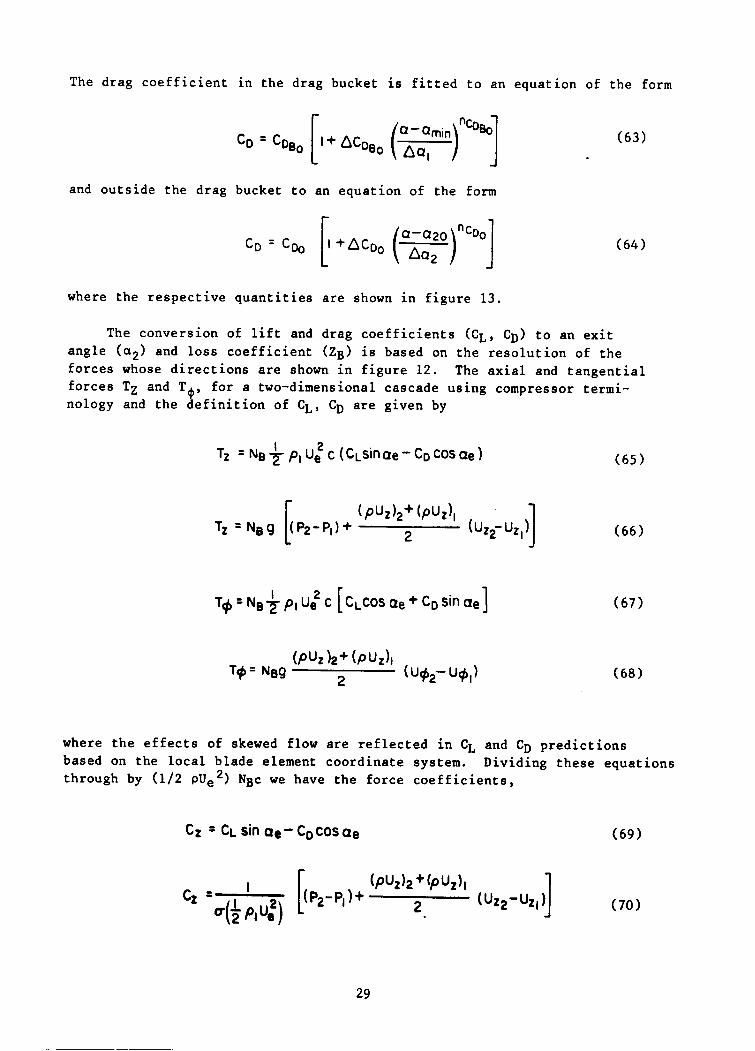
The drag coefficient in the drag bucket is fitted to an equation of the form

and outside the drag bucket to an equation of the form

where the respective quantities are shown in figure 13.

The conversion of lift and drag coefficients (CL, CD) to an exit angle ( a 2 ) and loss coefficient (ZB) is based on the resolution of the forces whose directions are shown in figure 12. forces TZ and T+, for a two-dimensional cascade using compressor termi- nology and the definition of CL, CD are given by

The axial and tangential

where the effects of skewed flow are reflected in CL and CD predictions based on the local blade element coordinate system. through by (1 /2 PUe2) NBC we have the force coefficients,

Dividing these equations

Cz = CL sin Qg- Co COS Qe (69)

29

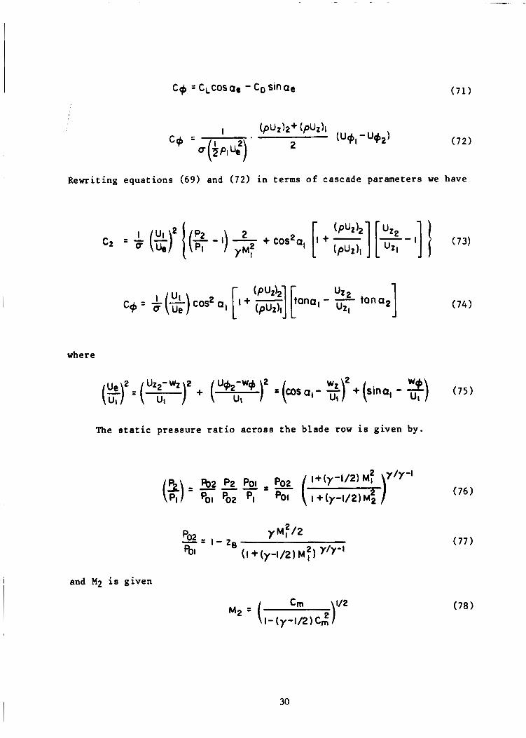
Rewriting equations (69) and ( 7 2 ) i n terms of cascade parameters we have

where

The s t a t i c pressure r a t i o across the blade row i s given by.

and M2 is given

30

where

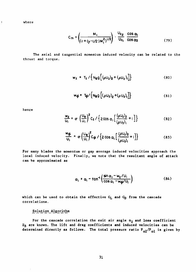
The axial and tangential momentum induced velocity can be related to the thrust and torque.

hence

For many blades the momentum or gap average induced velocities approach the local induced velocity. can be approximated as

Finally, we note that the resultant angle of attack

which can be used to obtain the effective CL and CD from the cascade correlations.

For the cascade correlation the exit air angle a2 and loss coefficient ZB are known. The lift and drag coefficients and induced velocities can be determined directly as follows. The total pressure ratio Po2/Pol is given by

31

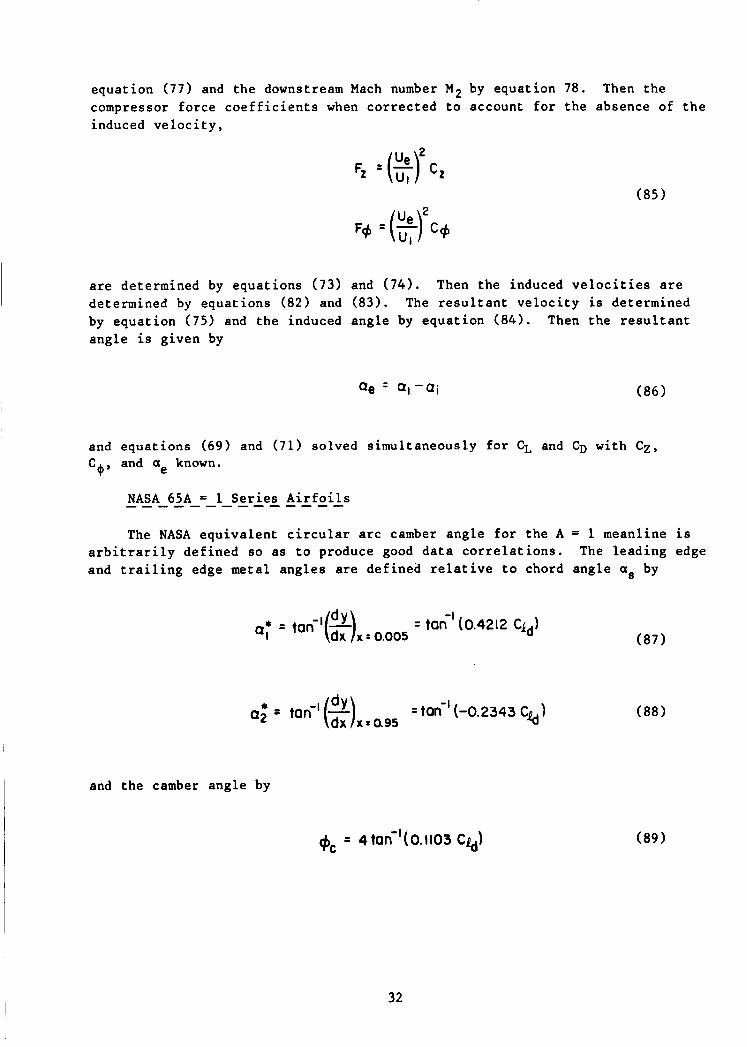
equation (77) and the downstream Mach number M p by equation 78. compressor force coefficients when corrected to account for the absence of the induced velocity,

Then the

are determined by equations (73) and (74). determined by equations (82) and (83). The resultant velocity is determined by equation (75) and the induced angle by equation (84). Then the resultant angle is given by

Then the induced velocities are

and equations (69) and (71) solved simultaneously for CL and CD with C z , C+, and ae known.

The NASA equivalent circular arc camber angle for the A = 1 meanline is arbitrarily defined so as to produce good data correlations. and trailing edge metal angles are defined relative to chord angle as by

The leading edge

and the camber angle by

32

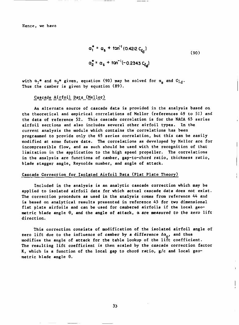
Hence, we have

with 01* and a2* given, equation (90) may be solved for as and cld. Thus .the camber is given by equation (89).

Cascade Airfoil Data (Mellgrl ------------- An alternate source of cascade data is provided in the analysis based on

the theoretical and empirical correlations of Mellor (references 49 to 51) and the data of reference 52. This cascade correlation is for the NACA 65 series airfoil sections and also includes several other airfoil types. In the current analysis the module which contains the correlations has been programmed to provide only the 65 series correlation, but this can be easily modified at some future date. The correlations as developed by Mellor are for incompressible flow, and as such should be used with the recognition of that limitation in the application to the high speed propeller. The correlations in the analysis are functions of camber, gap-to-chord ratio, thickness ratio, blade stagger angle, Reynolds number, and angle of attack.

Cascade Correction for Isolated Airfoil Data (Flat Plate Theory)

Included in the analysis is an analytic cascade correction which may be applied to isolated airfoil data for which actual cascade data does not exist. The correction procedure as used in the analysis comes from reference 44 and is based on analytical results presented in reference 45 for two dimensional flat plate airfoils and can be used for cambered airfoils if the local geometric blade angle 0, and the angle of attack, a are measured t o the zero lift direction.

This correction consists of modification of the isolated airfoil angle of zero lift due to the influence of camber by a difference Aao, and thus modifies the angle of attack for the table lookup of the lift coefficient. The resulting lift coefficient is then scaled by the cascade correction factor IC, which is a function of the local gap to chord ratio, g/c and local geometric blade angle 0.

33

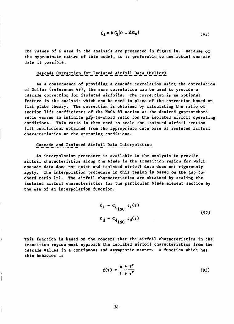
I The va lues of K used i n t h e a n a l y s i s are presented i n f i g u r e 14. 'Because of t h e approximate na tu re of t h i s model, i t i s p r e f e r a b l e t o use a c t u a l cascade d a t a i f p o s s i b l e . I

Cascade Cor rec t ion f o r I s o l a t e d A i r f o i l Data (Mel lor ) . . . . . . . . . . . . . . . . . . . . . . . . . . . A s a consequence of provid ing a cascade c o r r e l a t i o n us ing t h e c o r r e l a t i o n

o f Mel lor ( r e f e r e n c e 491, t h e same c o r r e l a t i o n can be used t o provide a cascade c o r r e c t i o n f o r i s o l a t e d a i r f o i l s . The c o r r e c t i o n i s an o p t i o n a l f e a t u r e i n t h e a n a l y s i s which can be used i n p l ace of t h e c o r r e c t i o n based on f l a t p l a t e t heo ry . s e c t i o n l i f t c o e f f i c i e n t s of t h e NACA 65 series a t the d e s i r e d gap-to-chord r a t i o ve r sus an i n f i n i t e g8p-to-chord r a t i o f o r t h e i s o l a t e d a i r f o i l o p e r a t i n g c o n d i t i o n s . Th i s r a t i o i s then used t o s c a l e t h e i s o l a t e d a i r f o i l s e c t i o n l i f t c o e f f i c i e n t ob ta ined from t h e a p p r o p r i a t e d a t a base of i s o l a t e d a i r f o i l c h a r a c t e r i s t i c s a t t h e o p e r a t i n g cond i t ions .

The c o r r e c t i o n i s obta ined by c a l c u l a t i n g t h e r a t i o of

Cascade and I s o l a t e d A i r f o i l Data I n t e r p o l a t i o n ........................ An i n t e r p o l a t i o n procedure is a v a i l a b l e i n t h e a n a l y s i s t o provide

a i r f o i l c h a r a c t e r i s t i c s a long t h e b lade i n t h e t r a n s i t i o n reg ion f o r which cascade d a t a does not e x i s t and i s o l a t e d a i r f o i l d a t a does not r i g o r o u s l y apply. The i n t e r p o l a t i o n procedure i n t h i s r eg ion i s based on t h e gap-to- chord r a t i o (T). The a i r f o i l c h a r a c t e r i s t i c s are obta ined by s c a l i n g t h e i s o l a t e d a i r f o i l c h a r a c t e r i s t i c s f o r t h e p a r t i c u l a r b l ade element s e c t i o n by t h e use of an i n t e r p o l a t i o n func t ion .

This func t ion is based on t h e concept t h a t t h e a i r f o i l c h a r a c t e r i s t i c s i n t h e t r a n s i t i o n r eg ion must approach the i s o l a t e d a i r f o i l c h a r a c t e r i s t i c s from the cascade va lues i n a continuous and asymptotic manner. t h i s behavior is

A func t ion which has

a + T~

1 + r n f ( r ) = ( 9 3 )

34

where t h e exponent (n) on t h e gap-to-chord r a t i o i s def ined by t h e use r . The va lue of t h e exponent c o n t r o l s t h e ra te a t which the func t ion a sympto t i ca l ly approaches u n i t y f o r l a r g e gap-to-chord r a t i o s . i n c r e a s e the r a t e . The va lue of t h e parameter ( a ) is determined i n t h e a n a l y s i s by t h e r a t i o of t h e cascade t o i s o l a t e d a i r f o i l c h a r a c t e r i s t i c s (Rc), where t h e cascade d a t a i s obta ined from the e x i s t i n g c o r r e l a t i o n s f o r a gap-to-chord r a t i o at t h e boundary of t h e c o r r e l a t i o n d a t a (a*).

Larger va lues of t h e exponent

a = R, + uBn ( ~ ~ - 1 ) (94)

This modeling o p t i o n can be used i n p l ace of t h e cascade c o r r e c t i o n f o r i s o l a t e d a i r f o i l s desc r ibed i n the previous s e c t i o n s .

35

Wake Modeling

The use o f a l i f t i n g l i n e model i n t h i s a n a l y s i s r e q u i r e s t h a t t h e wake geometry be prescr ibed f o r computat ional purposes. As noted ea r l i e r t h e wake i s r ep resen ted by a system o f t r a i l i n g v o r t e x f i laments . Within t h i s a n a l y s i s i t i s p o s s i b l e t o p r e s c r i b e i n t e r n a l l y s e v e r a l d i f f e r e n t wake geometr ies or input t h e wake geometry from an e x t e r n a l source. The reasons f o r t h i s v e r s a t i l i t y a r e twofold. F i r s t , a t t h e convent iona l ope ra t ing cond i t ions for t h e h igh speed p r o p e l l e r , t h e t r u e shape o f t h e wake i s not known, thus t h e need f o r t h e a b i l i t y t o inc lude a v e r s a t i l e range o f wake geometr ies . It i s however c lear t h a t t h e wake shape a t t h e s e speeds i s not s i g n i f i c a n t l y d i s t o r t e d . Secondly, a t low speed or s t a t i c f l i g h t cond i t ions t h e wake shape i s h i g h l y d i s t o r t e d as shown i n r e f e r e n c e 26, t h u s t h e need f o r wake models which can v a r y s i g n i f i c a n t l y i n shape i s w e l l documented. The use o f t h e a p p r o p r i a t e s e l e c t i o n o f t h e wake geometry model for t h e f l i g h t c o n d i t i o n under i n v e s t i g a t i o n i s important f o r accu ra t e p r o p e l l e r induced v e l o c i t y p r e d i c t i o n s . P r e f e r r e d wake models f o r t h e v a r i o u s f l i g h t speed regimes w i l l b e i n d i c a t e d . However, t h e f i n a l s e l e c t i o n o f wake model should be based on t h e r e s u l t s o f a wake s e n s i t i v i t y s tudy which remains t o be conducted i n f u t u r e a p p l i c a t i o n s o f t h e a n a l y s i s . a n a l y s i s are desc r ibed i n t h e fol lowing s e c t i o n s .

The wake models which can be used i n t h e

C l a s s i c a l Wake Model

E a r l y l i f t i n g l i n e models, for e i t h e r s t a t i c o r forward f l i g h t condi- t i o n s , g e n e r a l l y used what i s c a l l e d a c l a s s i c a l wake model. Th i s model c o n s i s t s o f d e f i n i n g t h e a x i a l wake t r a n s p o r t v e l o c i t y as t h e a d d i t i o n o f t h e forward speed and t h e momentum induced v e l o c i t y for t h e t h r u s t and f l i g h t c o n d i t i o n be ing i n v e s t i g a t e d .

No r a d i a l wake c o n t r a c t i o n i s used. The r e s u l t i n g wake shape i s an uncon- t r a c t e d h e l i x f o r which t h e p i t c h ra te depends on t h e f l i g h t c o n d i t i o n and t h r u s t l e v e l . F igure 15 i l l u s t r a t e s t h e model. This model can be used i n t h e a n a l y s i s f o r any f l i g h t cond i t ion . Although i t i s known t h a t f o r s t a t i c t h r u s t c o n d i t i o n s t h i s t ype o f wake model w i l l g i v e i n c o r r e c t answers, i t i s i n t h e a n a l y s i s because t h e self- induced d i s t o r t i o n s o f t h e p r o p e l l e r wake d e c r e a s e wi th forward speed. The c l a s s i c a l wake or t h e c l a s s i c a l wake as modif ied by s u p e r p o s i t i o n o f t h e n a c e l l e i n f luence ( t o be d i scussed ) can be used f o r t h e h igh speed p r o p e l l e r a p p l i c a t i o n .

Modified Classical Wake Model

V a r i a t i o n s of t h e c l a s s i c a l wake model can be used i n t h e a n a l y s i s i f d e s i r e d t o approximately account fo r bo th t h e n a c e l l e i n f luence and/or t h e

36

self-induced wake distortion. One model allows for a radially varying axial wake transport velocity which replaces the uniform value used in the classical wake model.

where the function fv(x) represents a spanwise velocity scaling distribution which varies radially along the blade. As in the classical wake model there is no radial wake contraction. The function fv(x) is normally obtained from knowledge of the nacelle influence at the blades. If desired, it can also account for the difference between the propeller self-induced velocity spanwise distribution and the momentum values. Figure 16 illustrates this wake model. The use of this model is assumed to be more representative of the wake of the high speed propeller nacelle configurations than that generated by a classical wake model. However, alternate procedures will be described.

Generalized Wake Model

For static thrust conditions, wake distortions are significant in terms of propeller performance predictions. Because of this fact, a wake model which has been shown to accurately model the statically thrusting propeller or hovering helicopter rotor wakes (reference 17 and reference 27) can be used in the analysis. This wake model is known as the generalized wake model. It is based on empirical results, and has radially varying axial wake transport velocities and radial contraction of the wake. Figure 16 illustrates the general character of this wake model for a statically thrusting propeller (see also figure 4). The wake geometry varies in both the axial and radial directions and is highly dependent on wake age, J;. the wake, $w, is the azimuth interval of blade rotation between the current blade azimuth and the azimuth at the time the wake point was emitted from the blade. A detailed explanation of the wake model is available in reference 17 or reference 26. The equations for the tip vortex coordinates normalized by the blade radius are noted below:

The wake age of a point in

in terms of the generalized wake parameters.

37

The cross sections of the vortex sheet from each blade are essentially lines rather than discrete points, as is the case for the tip vortex cross sections. The vortex sheet cross sections are assumed to be linear, the axial position of a vortex sheet at a given azimuth can be defined by two points. For simplicity, the two points are the imaginary extensions of the cross section to r = 0 at one end and to r = 1.0 at the other end, as shown in figure 17. These two points establish the intercept at the axis of rotation and the slope of the vortex sheet. It was assumed that the radial position of such intercepts (e.g., point A of figure 17) is linearly proportional to the radial coordinate of the intersection of the vortex sheet with the vortex sheet boundary (point B). blade (JI, < 2a/b), the vortex sheet boundary was assumed to be equivalent to the boundary formed by the locus centers of the tip vortex cross sections (equivalently, tip vortex streamline). 2a/b, the boundary was faired from the point of maximum circulation on the blade (point b of figure 17) to the tip vortex boundary. The constant of proportionality was assumed to be the ratio of the radial position of the origination of the filament streamline at the blade (point C) to the radial position of the vortex sheet boundary at the blade (point D). for the vortex sheet coordinates normalized by the blade radius are noted below:

With the exception of the immediate vicinity of the

For JIw less than the blade spacing,

The equations

The generalized wake coefficients (A,X,K1,K2,KlrP1,K2r=l,K2rPO) which define the wake shape must be determined in advance and input to the analysis. The values can be determined from experiment or from reference 17 for static propellers or reference 26 for hovering rotors.

38

Because t h e wake geometry must change smoothly from t h e h igh ly d i s t o r t e d shape under s t a t i c t h r u s t cond i t ions t o a b a s i c a l l y u n d i s t o r t e d shape a t h igh forward speeds wi th a n a c e l l e , t h e gene ra l i zed wake geometry noted above has t h e r a d i a l l y vary ing v e l o c i t y d i s t r i b u t i o n (neg lec t ing t h e momentum induced v e l o c i t y ) superimposed on i t t o account f o r t h e f l i g h t speed and t h e in f luence of t h e n a c e l l e . Thus i f t h e wake shape can be determined f o r low'forward speeds from some source of in format ion , i t i s expected t h a t t h i s model w i l l be u s e f u l i n modeling t h a t f l i g h t regime's wake c h a r a c t e r i s t i c s with t h e appro- p r i a t e input wake c o e f f i c i e n t s .

Nace l l e I n f l u e n c e s on t h e Wake Geometry

The presence of t h e p r o p e l l e r n a c e l l e can a l t e r t h e l o c a l flow a t t h e p r o p e l l e r b l a d e s and wake, p a r t i c u l a r l y nea r t h e n a c e l l e walls. model desc r ibed i n t h e Modified C l a s s i c a l Wake s e c t i o n i s based on t h e assump- t i o n t h a t t h e n a c e l l e does not i n f luence t h e r a d i a l l o c a t i o n of t h e wake geo- m e t r y and t h a t t h e a x i a l t r a n s p o r t v e l o c i t y i s cons t an t f o r a l l a x i a l Loca- t i o n s . I n r e a l i t y t h i s i s no t t h e case . I n t h e a n a l y s i s , i t i s p o s s i b l e t o apply a second approximate wake p e r t u r b a t i o n model which i s a f u n c t i o n o f t h e i n f l u e n c e of t h e n a c e l l e over t h e complete r eg ion e x t e r i o r t o t h e n a c e l l e boundary. This a l lows t h e wake t o a c c e l e r a t e and d e c e l e r a t e , expand or c o n t r a c t t o fo l low t h e flow around t h e n a c e l l e . This model i s based on t h e s u p e r p o s i t i o n o f t h e n a c e l l e ' s i n f luence ( e .g . , as determined from t h e n a c e l l e s t r e a m l i n e s o l u t i o n ) on one of t h e p rev ious ly desc r ibed wake models a8 used t o r e p r e s e n t t h e i s o l a t e d p r o p e l l e r wake. That i s , once a wake model i s s e l e c t e d f o r an i s o l a t e d p r o p e l l e r , t h e wake can be c o r r e c t e d f o r t h e presence of t h e n a c e l l e . The equa t ions f o r t h e n a c e l l e i n f luence are presented i n a l a t e r s e c t i o n (Nace l l e Wake Cor rec t ions ) . F igure 18 i l l u s t r a t e s t h i s concept. It i s recognized t h a t t h i s model, based on t h e p r i n c i p l e o f s u p e r p o s i t i o n i s on ly an approximation t o t h e a c t u a l wake. However, i t i s be l i eved t o be t h e most a c c u r a t e method a v a i l a b l e , s h o r t o f p r e s c r i b i n g empi r i ca l va lues from measured d a t a , which does no t r e q u i r e c a l c u l a t i n g t h e complete coupled p r o p e l l e r - n a c e l l e wake i n t e r a c t i o n problem numer ica l ly .

The wake

Wake Input Models

Since i t may be necessa ry t o p r e s c r i b e wake geometr ies which are no t compat ib le wi th any o f t h e c u r r e n t l y a v a i l a b l e wake models, t h e a n a l y s i s w i l l accept wake geometry inpu t compatible wi th t h e c y l i n d r i c a l c o o r d i n a t e system mentioned i n an e a r l i e r s e c t i o n . Thus, i f i t i s determined t h a t low or h igh speed f l i g h t c o n d i t i o n s r e q u i r e c u r r e n t l y unknown wake geometr ies f o r t h e p r o p e l l e r - n a c e l l e c o n f i g u r a t i o n s under c o n s i d e r a t i o n , t h e a n a l y s i s w i l l be a b l e t o accept t h e s e geometr ies .

39

Wake Rollup Modeling

The r e p r e s e n t a t i o n o f t h e wake o f a p r o p e l l e r b lade a s noted e a r l i e r c o n s i s t s o f modeling t h e shed shee t of v o r t i c i t y wi th d i s c r e t e v o r t e x f i l a - ments. The a c t u a l wake, however, i s known t o r o l l up i n t o a t i p v o r t e x and inboard s h e e t . The t i p v o r t e x h a s , i n g e n e r a l , a s t r e n g t h equal t o t h e maximum c i r c u l a t i o n s t r e n g t h on t h e b l ade , as shown i n f i g u r e 19. The occur- r ence o f a r o l l e d up r o o t v o r t e x has not been c l e a r l y demonstrated f o r hover ing r o t o r s or s t a t i c a l l y t h r u s t i n g p r o p e l l e r s , where wake d i s t o r t i o n s a r e most impor tan t . The modeling of t h i s phenomena, i f i t e x i s t s a t a l l , i s g e n e r a l l y not cons idered . impor tan t , i t i s g e n e r a l l y t h e d i s t o r t i o n o f t h e t i p v o r t e x which dominates t h e flow f i e l d c h a r a c t e r i s t i c s . I n t h e a n a l y s i s , i t i s poss ib l e t o p r e s c r i b e t h e wake r o l l u p f o r e i t h e r t h e inboard or t i p r e g i o n i f so d e s i r e d . o f t h e wake r o l l u p and t h e c o n c e n t r a t i o n o f c i r c u l a t i o n s t r e n g t h are d e t e r - mined from input q u a n t i t i e s . Genera l ly t h e t i p v o r t e x r o l l u p i s modeled t o occur w i t h i n 10 t o 15 degrees behind t h e b lade . The use of inboard wake r o l l - up i s not j u s t i f i e d from a phys ica l po in t of view a s noted above; however, f o r c o n d i t i o n s where a s i g n i f i c a n t l eng th of wake i s r equ i r ed ( s t a t i c t h r u s t ) i t i s p o s s i b l e t o reduce t h e computation t i m e i n t h e a n a l y s i s by s p e c i f y i n g inboard r o l l u p t o occur i n t h e f a r f i e l d wake without s a c r i f i c i n g computa- t i o n a l accuracy.

For cond i t ions where wake d i s t o r t i o n s a r e

The age

Vortex Core Modeling

I f i n t h e cour se o f t h e use o f t h i s a n a l y s i s , t h e p re sc r ibed wake model i s such t h a t a v o r t e x f i lament segment i s pos i t i oned c l o s e t o a f i e l d po in t (b l ade segment c e n t e r ) where t h e induced v e l o c i t y i s being c a l c u l a t e d , t h e p r e d i c t i o n s us ing t h e Biot-Savart Law f o r t h e magnitude o f t h e induced v e l o c i t y may exceed those which a c t u a l l y occur i n real l i f e f o r a d i s c r e t e l i n e v o r t e x such as t h e t i p v o r t e x or where t h e v o r t e x shee t i s modeled by d i s c r e t e v o r t e x f i l amen t s . To r e s o l v e t h i s problem, t h e a n a l y s i s i nc ludes a v o r t e x c o r e model which i s normally used. v a r i a t i o n o f t h e v e l o c i t y magnitude i n t h e c o r e i s cons t an t w i th v a r i a t i o n i n t h e d i r e c t i o n normal t o t h e f i l amen t segment and equal t o t h e v e l o c i t y a t a s p e c i f i e d c o r e r a d i u s . F igure 20 i l l u s t r a t e s t h i s model f o r a f i n i t e l e n g t h v o r t e x segment. Although it i s known t h a t t h e v e l o c i t y i n t h e c o r e o f a d i s c r e t e v o r t e x decays from t h e peak v a l u e a t t h e c o r e r a d i u s approximate ly l i n e a r l y t o ze ro a t t h e c e n t e r , t h i s s imple model i s f e l t t o be a s v a l i d as any o t h e r , on t h e b a s i s t h a t i f a c l o s e passage does occur , t h e modeling of t h e b l ade and wake by d i s c r e t e v o r t e x f i l amen t s i s i n i t s e l f i nappropr i a t e .

Th i s model assumes t h a t t h e

40

Compress ib i l i t y Cons idera t ions f o r Induced Ve loc i ty

When t h e performance o f two-dimensional a i r f o i l s i s found from t h e a i r - f o i l d a t a , t h e e f f e c t s o f c o m p r e s s i b i l i t y a r e inc luded , a s t h e d a t a i s tabu- l a t e d a s a f u n c t i o n of Mach number. To use t h e a i r f o i l d a t a f o r t h e c a s e where t h e p r o p e l l e r is o p e r a t i n g a t h igh forward Mach numbers, c o m p r e s s i b i l i t y e f f e c t s on t h e induced v e l o c i t y must a l s o be determined.

The c o n d i t i o n s f o r which t h e e f f e c t s of c o m p r e s s i b i l i t y on t h e induced v e l o c i t y need t o be cons idered are o u t l i n e d i n r e f e r e n c e 41. In summary, i f t h e l o c a l s e c t i o n Mach number ( t o t a l o f t h e r o t a t i o n a l and forward Mach numbers) a t t h e b l ade exceeds t h e l o c a l speed of sound, i t i s necessary t o cons ide r t h e e f f e c t s o f c o m p r e s s i b i l i t y on t h e induced v e l o c i t y . The proce- du re t o i n c o r p o r a t e t h e e f f e c t s o f c o m p r e s s i b i l i t y i s a l s o o u t l i n e d i n t h e above r e f e r e n c e f o r v o r t e x models. To compute t h e e f f e c t , i t i s necessary t o cons ide r t h e f i n i t e speed o f t h e p r e s s u r e d i s t u r b a n c e s i n comparison with t h e speed o f t h e b l ade s e c t i o n being analyzed. This l e a d s t o t h e r u l e of forb idden s i g n a l s when some o f t h e s e c t i o n s are o p e r a t i n g a t s e c t i o n Mach numbers above one. Thus t h e e f f e c t s o f t h e l i n e v o r t e x shed from a s e c t i o n o p e r a t i n g a t a s e c t i o n Mach number above one a r e cons idered only a t p o i n t s i n t h e r e g i o n o f i t s a f t Mach cone, where t h e apex o f t h e Mach cone i s a t t ached t o t h e s e c t i o n from which t h e l i n e v o r t e x i s shed on t h e p r o p e l l e r b l ade . F igure 21 (from r e f e r e n c e 41) i s a p i c t o r i a l r e p r e s e n t a t i o n of t h i s concept and i l l u s t r a t e s t h e b l ade and Mach cone which d e f i n e s t h e l i m i t s o f t h e p o s s i b l e induced in f luence o f t h e t r a i l i n g l i n e vo r t ex . For t h e case o f a h igh speed p r o p e l l e r o p e r a t i n g wi th b l a d e s e c t i o n Mach numbers g r e a t e r than one bu t forward Mach numbers less than one, t h e i n i t i a l p o r t i o n of t h e t r a i l - ing l i n e v o r t i c e s shed from t h e s e b l ade s e c t i o n s w i l l have no in f luence a t t h e p r o p e l l e r b l ades . However, a f t e r some f i n i t e per iod o f t i m e t h e in f luence o f a p o r t i o n o f t h e l i n e v o r t e x w i l l r each t h e p r o p e l l e r d i s k . F igure 22 ( a l s o from r e f e r e n c e 41) i l l u s t r a t e s t h i s concept , where t h e p o s i t i o n of t h e b lade and t h e Mach cone boundary a r e p l o t t e d f o r d i f f e r e n t r o t a t i o n a l p o s i t i o n s o f t h e b l ade ( t i m e ) . It i s shown i n t h i s f i g u r e t h a t f o r a forward Mach number less t h a n one, t h e induced in f luence o f a p o r t i o n of t h e l i n e v o r t e x does e v e n t u a l l y r each t h e b lade a f t e r some f i n i t e t i m e (between t i m e C and D i n f i g u r e 2 2 ) .

To c a l c u l a t e t h e induced inf low v e l o c i t y o f a p r o p e l l e r o p e r a t i n g a t a t i p Mach number exceeding one and a forward Mach number less than one, i t i s necessa ry t o e v a l u a t e t h e e f f e c t s o f t h e t r a i l i n g v o r t i c e s t h a t l i e i n t h e zone o f i n f l u e n c e on ly . e f f e c t s o f t h e v o r t i c e s are cons idered from t h e p r o p e l l e r p lane t o i n f i n i t y i n s t a n t a n e o u s l y , i t becomes necessa ry t o d i s c r i m i n a t e a g a i n s t t h e e f f e c t s of t h e v o r t i c e s o u t s i d e t h e zone o f i n f l u e n c e o r t h e Mach cone as shown i n f i g u r e 21. on a b l ade segment a t a p a r t i c u l a r t i m e should not be cons idered when t h e

Thus, u n l i k e t h e incompress ib le flow case where

Thus t h e p o r t i o n o f t h e t r a i l i n g v o r t e x f i l a m e n t s which h a s no i n f l u e n c e

41

calculation of the geometric influence coefficients using the Biot-Savart Law is made as noted in the section entitled: Lifting Line Theory. This approach has been included in the analysis. The concept of the induced influence of a trailing line vortex limited by compressibility considerations can also be applied to the bound vortex segments representing the blade. The validity of applying this concept to the bound vortex influence has not been established; however, it is available in the analysis if so desired.

As noted above, the reference 41 assumes inf

concept of wake compressibility as outlined in nite propagation of the induced field of the trailing

line vortices shed from blade sections operating at section Mach numbers less than unity and finite propagation (speed of sound) of the induced influence when the sections are operating at section Mach numbers greater than unity. A second feature, which is not normally used, is provided in the analysis for exploring the influence of finite rather than infinite propagation speed for blade sections with a section Mach number less than one. That is, a provision is included which assumes that the influences of all bound and/or trailing wake elements propagate at the speed of sound.

42

Coaxial Theory - Equal Blade Number and Ro ta t iona l Speeds

For t h e c o a x i a l , c o u n t e r - r o t a t i n g p r o p e l l e r a n a l y s i s , t h e assumption of an axisymmetric s t eady s t a t e flow problem wi th r e s p e c t t o t h e b l ade coord ina te system must be removed. I n t h e b l ade c o o r d i n a t e system, t h e c i r c u l a t i o n solu- t i o n becomes p e r i o d i c w i t h h a l f b l ade spac ing f o r equal b l ade number and r o t a t i o n a l speeds. This f e a t u r e i s demonstrated i n f i g u r e 23 where i t can be seen t h a t t h e geometry of t he problem i s p e r i o d i c wi th h a l f b l ade spacing. The h a l f b l ade spac ing i s t h e azimuthal i n t e r v a l o f b l ade r o t a t i o n between t h e two p r o p e l l e r s r e q u i r e d f o r t h e r e l a t i v e geometry t o r epea t i t s e l f . o f l i f t i n g l i n e t h e o r y i s s t i l l v a l i d w i t h i n t h e c o n s t r a i n t s of t h e o t h e r assumptions noted i n ear l ier s e c t i o n s . concep tua l d i f f e r e n c e between t h e s i n g l e and c o a x i a l s o l u t i o n s a t t h e b lade rowa i s t h e above noted p e r i o d i c i t y . s t e a d y aerodynamics. b l a d e c i r c u l a t i o n s only need t o be modified t o inc lude t h e s o l u t i o n period- i c i t y . r e s u l t i n g r e l a t i o n s h i p s are r ep resen ted h e r e i n .

The use

In t h i s a n a l y s i s t h e on ly major

The c o a x i a l a n a l y s i s asrumes quas i - Thus t h e r e l a t i o n s h i p s used t o determine t h e unknown

The d e t a i l s o f such a d e v i a t i o n a r e s t r a i g h t f o r w a r d and on ly t h e

Coordina te Systems

Within t h e c o a x i a l l i f t i n g l i n e a n a l y s i s , d e f i n i t i o n s o f t h e c o o r d i n a t e systems are i d e n t i c a l w i th t h o s e i n t h e s i n g l e p r o p e l l e r a n a l y s i s . C a r t e s i a n and c y l i n d r i c a l c o o r d i n a t e systems are r e fe renced wi th r e s p e c t t o each b l a d e row, w i t h t h e d e f i n i t i o n s o f p o s i t i v e q u a n t i t i e s c o n s i s t e n t w i th t h e r e s p e c t i v e d i r e c t i o n o f r o t a t i o n o f each b l ade row. I n t h e a n a l y s i s t h e r e i s no d i s t i n c t i o n between which b l a d e row i s r o t a t i n g i n which d i r e c t i o n , o n l y t h a t t h e y are c o u n t e r - r o t a t i n g ; t h i s i s because t h e problem i s symmetric i n n a t u r e . w i t h t h a t b l a d e row's c o o r d i n a t e system. noted c o o r d i n a t e systems. t h a t t h e hubs o f t h e two p r o p e l l e r s be sepa ra t ed by a f i n i t e axial d i s p l a c e - ment. P r o p e l l e r one ( i n terms o f input o r d e r i n g ) i s assumed t o l i e i n f r o n t of p r o p e l l e r two, and a p o s i t i v e hub displacement p o s i t i o n s p r o p e l l e r t w o behind p r o p e l l e r one ( f i g u r e 24). The b l a d e element c o o r d i n a t e system for each b l ade row i s c o n s i s t e n t w i th t h e r e s p e c t i v e C a r t e s i a n and c y l i n d r i c a l c o o r d i n a t e systems.

The

The d e f i n i t i o n s o f v e l o c i t i e s computed a t a b l a d e row are c o n s i s t e n t F igure 24 i l l u s t r a t e s t h e above

For c a l c u l a t i o n purposes, t h e a n a l y s i s r e q u i r e s

L i f t i n g Line Theory

As noted e a r l i e r , t h e a d d i t i o n o f a coun te r - ro t a t ing p r o p e l l e r r e q u i r e s t h e i n c l u s i o n o f geometric p e r i o d i c i t y and hence c i r c u l a t i o n p e r i o d i c i t y i n t h e r e l a t i o n s h i p s used t o compute t h e s o l u t i o n . For t h e c a l c u l a t i o n o f t h e induced v e l o c i t y a t a f i e l d po in t u s i n g l i f t i n g l i n e theo ry , t h e r e l a t i o n s h i p s

4 3

derived earlier must be expanded to include the periodic nature of the circulation solution of each blade row and the wake influence. The resulting relationship for a component of induced velocit-y, in this case the normalwise component, at an arbitrary field point is:

where it is assumed that there are identical number of blade stations (N) at each blade row and that there are L propeller positions between half blade spacings for a given blade azimuth step size. The term, propeller position, means the discrete azimuthal location of the propeller within a specified rotational interval, defined by a finite azimuthal step size. In this case, the interval is the half blade spacing, and the discrete azimuthal locations are defined by the azimuthal wake segmentation interval.

Blade Element Aerodynamics

The effect of including a second propeller blade row on the aerodynamic relationships is to expand the number of unknown bound circulation strengths, and hence the size of the matrix of equations which must be solved using either the linear or nonlinear solution. The relationship for the unknown circulation at station i for propeller position j of propeller p for the nonlinear solution becomes:

(103

where the correction term CVT! coaxial propeller condition. term yields the linear solution. circulation at each station on each propeller blade for each propeller position a matrix of NxLx2 simultaneous equations can be written, and the same solution methods can be applied as for the single propeller condition.

has the appropriate modifications for the Eropping the superscripts and the correction

F1 J

From this relationship for the unknown bound

The resulting blade forces can be computed and integrated for each propeller at each propeller position. the propeller positions to obtain the steady thrust and torque. nacelle code these steady forces are the values used for the coaxial case since the nacelle analysis assumes steady flow conditione..

The resulting values can be averaged over For the

44

Other Considerations for Coaxial Propellers

The use of the different wake models and airfoil data for the coaxial propeller configuration is the same for the single propeller configuration. There is only one restriction in the analysis which limits the use of these portions of the analysis to single propeller configurations. is the application of the rule of forbidden signals to the bound vortex which is noted in the section entitled: Compressibility Considerations on the Induced Velocity Calculation. The analysis will not allow the application of this modeling feature to the coaxial configuration. The reason is that the formulation for this model as applied to the bound vortex has not been developed for the coaxial configuration because this model is in itself questionable.

That restriction

Because the wake of the leading propeller can pass close to the lifting line representation for the blades on the following propeller, care should be taken to inspect the resultant blade loadings to look for large gradients in loading due to close blade-vortex interactions. The validity of the solutions where these close passages occur is questionable. The use of different core radii for the wake vortex systems can influence the answers when these close passages occur, and so careful selection of the appropriate values should be made for the coaxial configuration.

45

Coaxial Theory - Unequal Blade Number and Rotational Speeds

For the coaxial configuration, the introduction of unequal number of

The concept of periodicity of the blades and unequal rotation speeds on the propeller disks creates-an additional complexity in the analysis. propeller bladelwake geometry and periodicity of the circulation solution still exists, but the definition of azimuthal interval must be replaced with a time interval as the quantity which defines this periodicity. This is due to the fact that the propeller blades do not necessarily rotate at the same speed. In general, it can be shown that the time interval for which the propeller blade and wake geometry are periodic is,

2n e = (104)

where b is the maximum of the number of blades on each of the propeller disks. This relationship reduces to the conventional one for coaxial propellers with equal number of blades and rotational speeds on each disk; the periodic azimuthal interval is one half of the blade azimuth interval.

The relationships for the formulation of the numerical solution procedure are no different than those for the conventional coaxial configurations. However, the implementation of the formulation in the computer code must be made in terms of time intervals instead of azimuth intervals. For unequal rotational speeds on the propellers, this results in different azimuth intervals used to define the propeller positions and wake geometries.

The analysis includes this feature to treat the unequal number of blades and rotational speeds with certain limitations. These limitations are related to computer program storage requirements and are not conceptual in nature. Large variations between the number of blades on each propeller disk, or large variations in rotational speeds, result in periodic time intervals which require a large number of unknowns in the solution formulation. This increase in the number of unknowns increases the physical storage needed in the program and the computational time required to obtain the solution. analysis is limited to combinations of blade number and rotational speed which result in periodic time intervals with corresponding azimuthal intervals on the respective propeller disks of no less than five (5.0) degrees. This limitation can be relaxed by re-dimensioning the computer code if deemed necessary at some future time. The analysis controls the selection of the actual time increments used in the definition of the wake geometries based on

The current

46

t h e p e r i o d i c t i m e i n t e r v a l r e l a t i o n s h i p def ined above. t o f ind a t i m e increment which is a t l e a s t one t h i r d of t h e p e r i o d i c t i m e i n t e r v a l f o r t h e p a r t i c u l a r s e l e c t i o n of b lade numbers and r o t a t i o n a l speeds and which does not r e s u l t i n an azimuthal i n t e r v a l f o r e i t h e r p r o p e l l e r less than t h e c u r r e n t l i m i t of f i v e degrees. i n t e r v a l t o r e s u l t i n an azimuthal i n t e r v a l on e i t h e r p r o p e l l e r which i s not g r e a t e r than a s p e c i f i e d va lue .

The a n a l y s i s a t t empt s I

The u s e r can a l s o l i m i t t h e t i m e

The a n a l y s i s has been coded i n such a manner t h a t t h e unequal b l ade number and r o t a t i o n a l speed f e a t u r e does not resul t i n a s i g n i f i c a n t computer overhead pena l ty when app l i ed t o t h e more convent iona l o r c o a x i a l o p e r a t i n g c o n f i g u r a t i o n s .

47

TECHNICAL APPROACH - NACELLE

Overview

A l a r g e and important c l a s s o f problems i s r ep resen ted by vi6cous t u r b u l e n t flows over axisymmetric n a c e l l e s with t h e fo l lowing p r o p e r t i e s : 1) moderate t o h igh Reynolds numbers, 2) s t rong invisc id-v iscous i n t e r a c t i o n s , 3) l a r g e r eg ions o f i n v i s c i d f lows , and 4 ) s i g n i f i c a n t " e l l i p t i c " e f f e c t s d u e t o s t r e a m l i n e c u r v a t u r e and s t r eaml ine divergence. c a l c u l a t i o n of such flows i s of immediate and p r a c t i c a l i n t e r e s t i n t h e p r e d i c t i o n of flows over a n a c e l l e f o r e i t h e r e x t e r n a l or i n t e r n a l flow.

Accurate and r e l i a b l e

This s e c t i o n c o n s i s t s o f s e v e r a l p a r t s . F i r s t , a procedure i s presented f o r c o n s t r u c t i n g an or thogonal coord ina te system from t h e p l ana r p o t e n t i a l f low s o l u t i o n us ing t h e stream func t ion a s a normal coord ina te and t h e ve loc- i t y p o t e n t i a l a s t h e streamwise coord ina te . Since t h e p o t e n t i a l flow stream- l i n e s approximate t h e v i scous flow s t r e a m l i n e s , t h e t h i n channel approxima- t i o n , r e f e r e n c e s 4 and 5 , may be app l i ed t o t h e Navier-Stokes equa t ions w r i t t e n i n t h i s p o t e n t i a l flow coord ina te sys tem t o reduce them t o a set of p a r a b o l i c equa t ions which can be solved by forward marching numerical methods. Second, a method us ing conformal mapping based on t h e Schwar tz -Chr is tof fe l t r ans fo rma t ion i s presented f o r o b t a i n i n g t h e p lane p o t e n t i a l flow s o l u t i o n f o r t h e flow over an a x i s p e t r i c n a c e l l e . This procedure has t h e important p rope r ty t h a t t h e i n v e r s e s o l u t i o n i s obta ined d i r e c t l y through t h e t r a n s f o r - mation so t h a t e q u i p o t e n t i a l l i n e s and s t r eaml ines can be used t o c o n s t r u c t t h e c o o r d i n a t e s . scheme i s presented f o r so lv ing t h e v i scous flow equa t ions . It should be noted h e r e t h a t t h e term, d u c t , i s used even when cons ide r ing t h e e x t e r n a l f low problem o f t h e p rope l l e r -nace l l e geometry. For t h e s e e x t e r n a l flow problems, t h e o u t e r w a l l o f t h e duc t becomes t h e o u t e r l i m i t f o r t h e computa- t i o n a l r e g i o n wi th t h e a p p r o p r i a t e mod i f i ca t ions t o t h e boundary c o n d i t i o n s , and t h e i n n e r w a l l becomes t h e n a c e l l e p r o f i l e . And f i n a l l y , because of t h e p a r t i c u l a r requi rements o f t h e n a c e l l e a p p l i c a t i o n , s t r e a m l i n e c u r v a t u r e c o r r e c t i o n s t o t h e t h i n channel approximation are necessa ry ( r e f e r e n c e 5 3 ) and a r e included i n t h e a n a l y s i s .

Thi rd , a s o l u t i o n a lgor i thm based on t h e two po in t box

PRECEDING PAGE BLANK NOT FILMED

49

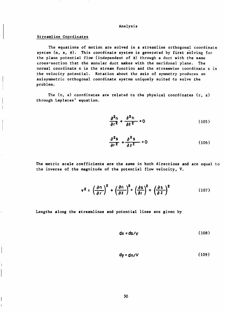
Ana 1 y s is

Streamline Coordinates

The equations of motion are solved in a streamline orthogonal coordinate system (n, s, $1. This coordinate system is generated by first solving for the plane potential flow (independent of $1 through a duct with the same cross-section that the annular duct makes with the meridonal plane. The normal coordinate n is the stream function and the streamwise coordinate s is the velocity potential. Rotation about the axis of symmetry produces an axisymmetric orthogonal coordinate system uniquely suited to solve the problem.

The (n, s) coordinates are related to the physical coordinates (r, z ) through Laplaces' equation.

The metric scale coefficients are the same in both directions and are equal to the inverse of the magnitude of the potential flow velocity, V.

Lengths along the streamlines and potential lines are given by

dx =ds/v

dy = dn/v

(108)

(109 1

50

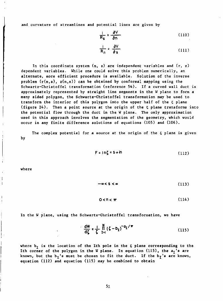
and curvature of streamlines and potential lines are given by

I av - = - RS an

(110)

In this coordinate system (n, s) are independent variables and (r, z) dependent variables. While one could solve this problem numerically, an alternate, more efficient procedure is available. Solution of the inverse problem (r(n,s), z(n,s)) can be obtained by conformal mapping using the Schwartz-Christoffel transformation (reference 54). If a curved wall duct is approximately represented by straight line segments in the W plane to form a many sided polygon, the Schwartz-Christoffel transformation may be used to transform the interior of this polygon into the upper half of the 5 plane (figure 24). Then a point source at the origin of the 5 plane transforms into the potential flow through the duct in the W plane. The only approximation used in this approach involves the segmentation of the geometry, which would occur in any finite difference solutions of equations (105) and (106).

The complex potential for a source at the origin of the 5 plane is given by

where

In the W plane, using the Schwartz-Christoffel transformation, we have

I (115 1

where bI is the location of the Ith pole in the 5 plane corresponding to the Ith corner of the polygon in the W plane. known, but the bits must be chosen to fit the duct. equation (112) and equation (115) may be combined to obtain

In equation (1151, the aIts are If the bits are known,

51

(116)

Integration of equation (116) with n constant, produces a streamline, and integration of equation (116) with 8 constant, produces a potential line. The metric scale coefficient is equal to the inverse of the magnitude of the potential flow velocity and is given by

(117)

The unknown bI's are determined iteratively by comparing the calculated length along each wall with the actual length. In the 5 plane, the inner wall cooresponds to n = 0 and the outer wall to n = TI as shown in figure 25. However, since the poles also lie on the 5 axis, the numerical integration of the wall contour using equation (116) is obtained by setting n = E and II = E .

Hence for bI assumed, the calculated length along each wall for the vth iteration and Ith pole is

(118)

The actual length along the wall to the Ith pole is known and given by

and the error in calculating the location of the Ith pole is

(119)

(120)

Therefore, to minimize the error by Newton's method, we have from equation (118) and equation (119) the recursion formula

52

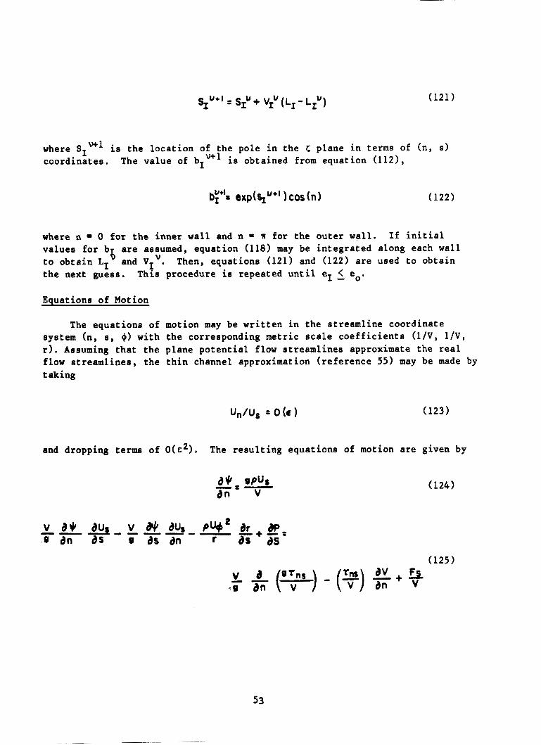
where SIw1 is the location of the pole in the C plane in terms of (n, 8 )

coordinates. The value of bIW1 is obtained from equation (1121,

where n = 0 for the inner wall and n n for the outer wall. If initial values for b to obtain LI the next guess.

are assumed, equation (118) may be integrated along each wall and V I v . 6 Then, equations (121) and (122) are used to obtain

This procedure is repeated until eI < eo. - Equations of Motion

The equations of motion may be written in the streamline coordinate system (n, 8 , 4) with the corresponding metric scale coefficients (l/V, 1/V, r). Assuming that the plane potential flow streamlines approximate the real flow streamlines, the thin channel approximation (reference 55) may be made by taking

and dropping t e r m of O(c2) , The resulting equations of motion are given by

53

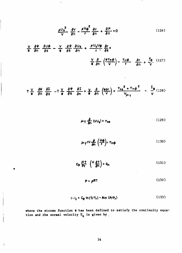
(126)

P = pRT (132)

where the stream function Q has been defined to satisfy the continuity equation and the normal velocity Un is given by ,

54

Equations (124) through (133) form a set of eight first order parfial differential equations and two algebraic equations which may be used to solve for ten unknowns. The boundary conditions for this problem are given by

(135)

for the inner wall and

= Uo (External flow)

for the outer wall.

The remaining unknown is the viscosity. For laminar flow, Sutherlands law is used to obtain the molecular viscosity dT). empirical relations are used to obtain the effective turbulent viscosity UT.

For turbulent flow

55

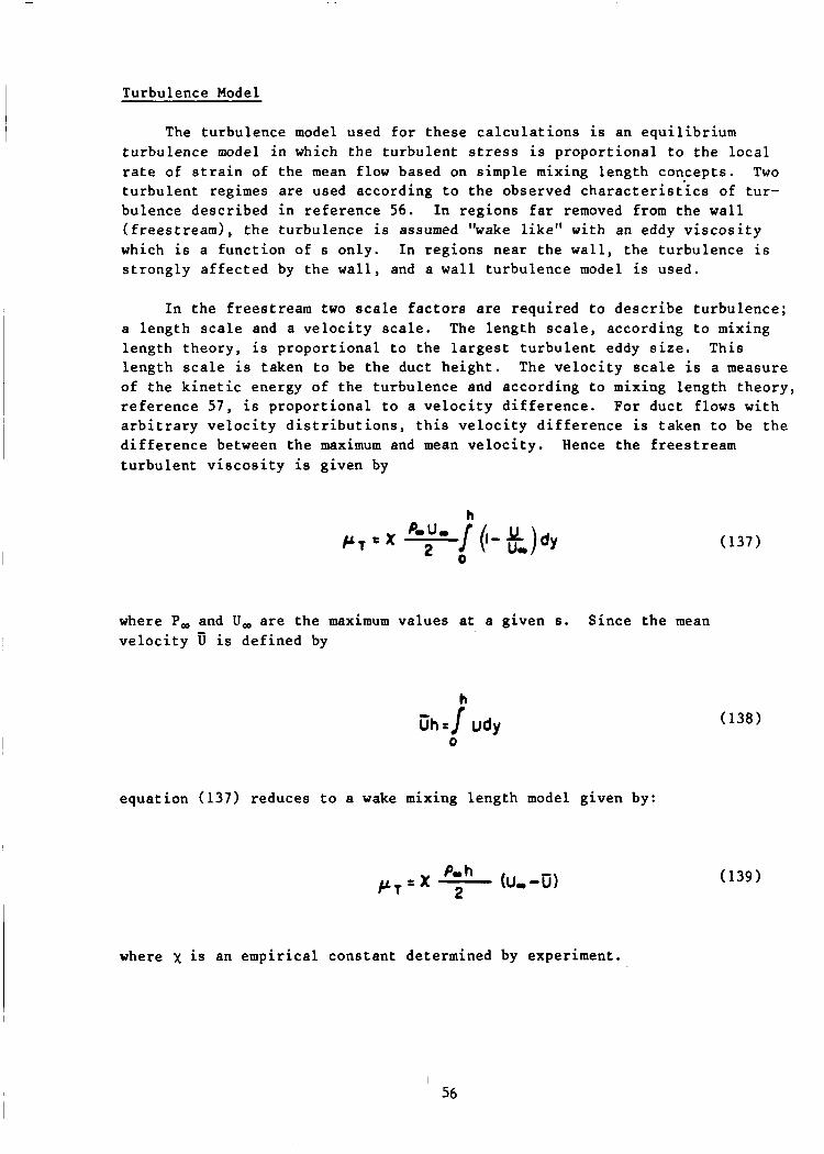
Turbulence Model

The turbulence model used f o r these c a l c u l a t i o n s i s an equ i l ib r ium turbulence model i n which the tu rbu len t stress i s propor t iona l t o the l o c a l r a t e of s t r a i n of t he mean flow based on simple mixing length concepts . Two tu rbu len t regimes are used according t o t h e observed c h a r a c t e r i s i i c s of t u r - bulence descr ibed i n r e fe rence 5 6 . I n regions f a r removed from the w a l l ( f r ees t r eam) , t h e turbulence is assumed "wake l ike" with an eddy v i s c o s i t y which is a func t ion of s only. I n regions near t he wal l , t he turbulence i s s t r o n g l y a f f e c t e d by the wa l l , and a wal l tu rbulence model i s used.

I n the f rees t ream two scale f a c t o r s are requi red t o desc r ibe turbulence ; a length s c a l e and a v e l o c i t y s c a l e . The length s c a l e , according t o mixing length theory , i s p ropor t iona l t o the l a r g e s t t u rbu len t eddy s i z e . Th i s length s c a l e i s taken t o be t h e duct he igh t . The v e l o c i t y s c a l e i s a measure of t he k i n e t i c energy of t he turbulence and according t o mixing length theory , r e f e r e n c e 5 7 , i s p ropor t iona l t o a v e l o c i t y d i f f e r e n c e . For duct flows wi th a r b i t r a r y v e l o c i t y d i s t r i b u t i o n s , t h i s v e l o c i t y d i f f e r e n c e i s taken t o be t h e d i f f e r e n c e between t h e maximum and mean v e l o c i t y . Hence the f r ees t r eam tu rbu len t v i s c o s i t y i s given by

h

J (I- k ) d y 2 0

P r = X

where P, and U, are t h e maximum values a t a given s. Since t h e mean v e l o c i t y i s def ined by

h

equat ion (137) reduces t o a wake mixing length model given by:

where x is an empi r i ca l cons tan t determined by experiment.

(137)

1 56

Near the wall, the turbulence model derived by Van Driest (reference 5 8 ) is used.

where U+ and Y+ are defined by

u'= u / q (141)

Two empirical constants are used K and A+ which are taken to be 0.40 and 26.0, respectively.

The empirical constant x remains to be determined. It is noted that two boundary layers exist in the duct. Hence for uniform freestream flow, equation (137) reduces to

* where 6 is the boundary layer displacement thickness. The value for x has been obtained by Clauser (reference 5 9 ) and is taken to be 0.016.

Initial Conditions

The initial conditions for this problem require specification of all dependent variables $, Us, U+, P, p , T, I, T , , ~ ,

n+' In the freestream, it is assumed that T ~ ~ , T zero. To(n), $(n) using the isentropic flow relations and equations (124) and (126) to insure that the continuity equation and radial momentum equation are satisfied.

qn as a function of n. 21' qn, flow swirl angle are Then the remaining variables are uniquely defined by Po(n), B(n),

In the nacelle boundary layer, ~ ~ ~ ( n ) , Tn+(n), qn(n) must be specified in such a manner as to be consistent with the turbulence model. This is accomplished by using Coles' law (reference 60) for the mean velocity profile assuming colateral flow ( B = constant). Thus we have

57

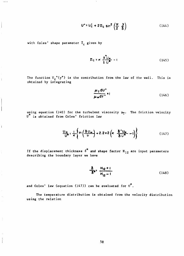
with Coles' shape parameter lIc given by

r( 6 U e n c = c c - - , - t 6 U (145 1

The function Uc+(y+) is the contribution from the law of the wall. obtained by integrating

This is

PT dU'

p w d y ' - 'I (146)

using equation (140) for the turbulent viscosity h. U is obtained from Goles' friction law

The friction velocity *

* If the displacement thickness 6 describing the boundary layer we have

and shape factor H 1 2 are input parameters

* and Coles' law (equation (147)) can be evaluated for U . The temperature distribution is obtained from the velocity distribution

using the relation

58

T and q are obtained With the mean boundary layer profiles calculated, T ~ ~ , using the relations for turbulent viscosity and stress (equations (129) to (131) and (140)).

n4 n

Inviscid Flow Calculation

The solution for the inviscid flow around the nacelle is used to calculate the propeller wake corrections due to the influence of the nacelle on the propeller wake and is also used to calculate the influence of the nacelle on the flow at the lifting line.

For inviscid flows with no work or heat addition, the total temperature To, total pressure Po, and angular momentum (rU are conserved streamlines. These quantities, however, may vary from streamline to streamline. Therefore along a streamline the isentropic flow relations may be used. Furthermore, since the coordinate n is the stream function for the potential flow around the nacelle, the curve n(r,z) flow Streamlines. @ Thus the following equations can be used to calculate the solution for the inviscid flow.

4

no approximates the inviscid Hence Po, To, and (rU are functions of n only.

Y

59

In addition the inviscid flow must satisfy the continuity equation, equation ( 1 2 4 1 , and the normal momentum equation, equation (126).

which may be expressed as

d q - Pus dn V

- - - (153)

The solution of equations (153) through (156) produces the inviscid compressible flow field. This solution is obtained by the following transformation of variables.

Let

Y- I x = (7)- Po Y

and

(157)

60

Equation (109) becomes

which is an ordinary first order linear equation.

The solution is given by

n #(n)= expl J ody + nn (&)I 0

The boundary conditions for the solution of the problem are:

I J/(o) = 0 P( I) = Pa

(159)

(160)

(161)

(162)

(163)

For the case of the nacelle in a wind tunnel, the boundary conditions are:

( 1 6 4 )

since mass flow is conserved in the tunnel.

61

Per fo ra t ed Wall Bleed Model

For some tunne l s , t he use of a zero normal flow boundary cond i t ion i s i n a p p r o p r i a t e when t h e tunnel i s run using b leed . be modeled as descr ibed below.

This type of ope ra t ion can

I f one t reats a s i n g l e ho le i n a pe r fo ra t ed w a l l a s an o r i f i c e , then t h e mass flow can be der ived i n terms of t he plenum s t a g n a t i o n cond i t ions and the l o c a l s t a t i c p re s su re i n s i d e the tunne l , Holman ( r e f e r e n c e 61) . exp res s ion f o r t h e mass flow added t o the tunnel flow is given by

Then an

(PU,), = c - I)] 1"' (165)

where PT and TT are t h e plenum cond i t ions , P i s t h e l o c a l tunnel s t a t i c p r e s s u r e , %/A8 i s t h e r a t i o of t h e hole a r e a t o su r face a r e a , and C t h e e f f e c t i v e d i scha rge c o e f f i c i e n t which i s a proper ty of t h e pe r fo ra t ed w a l l . I f t h e tunnel s t a t i c p r e s s u r e is g r e a t e r than t h e plenum t o t a l p r e s s u r e , t h e mass flow bleed is are taken from t h e i s assumed known.

The mass flow

ou t of the tunnel . Under these cond i t ions , PT and TT wind tunnel cond i t ions , and P i s t h e plenum pres su re which

b leed is r e l a t e d t o the stream func t ion by

Equations (165) and (166) provide t h e boundary cond i t ions f o r a p e r f o r a t e d w a l l r e l a t i n g two dependent v a r i a b l e s J' and P i n terms of t he c h a r a c t e r i s t i c s of t h e p e r f o r a t e d wall and t h e plenum cond i t ions .

S ince p e r f o r a t e d walls have very high r a t e s of b leed which suck o f f o r blow o f f t h e boundary l a y e r , t h e boundary cond i t ions were taken t o be

T - 0 n8KL

(168)

(169)

62

Nacelle Wake Corrections

The presence of the nacelle can significantly alter the velocity distribution at the propeller blade. The flow, and hence the streamline, can accelerate or decelerate to follow the shape of the nacelle. Thus if a wake model is known for an isolated propeller, then the isolated wake should be corrected for the presence of the nacelle by addition of the nacelle's influence on the streamline due to its presence in the flow (figure 18).

The nacelle wake corrections are determined by comparing the calculated streamlines for the flow over the nacelle to the classical wake streamlines. Since the vorticity shed from the lifting line is convected by the streamlines, the location of a vortex element is given by

z = ZO+Ucot (170)

for the classical wake where U, is the freestream velocity and 0 the propeller rotational speed. The location of the vortex filament in the flow field about the nacelle is given by:

t z = z,+ j u,dt ( 1 7 3 )

0

( 1 7 4 )

( 1 7 5 )

63

The wake corrections (displacement from classical wake) for each streamline passing through the lifting line at the point ro is given by

Since the lifting line theory uses qW as in independent variable referenced to the blade at t = o ( Q 0 0 ) .

t q,,, = 1 f ld t

0

where the dimensional time is

ds "US

dt = -

(179)

(180)

and V is the metric scale coefficient.

Blade Force

The action of the propeller blades on the circumferential average flow is treated by using body forces (force/volume) in the streamwise and tangential momentum equations, equations (125) and (127) and by using a dissipation function in the energy equation, equation (128). A rigorous derivation of these terms is given in reference 5.

64

The forces produced by the propeller are calculated using lifting line theory as derived in the propeller portion of the report. These forces (force/span) act on the lifting line and are resolved in the axial, tangential, and radial direction so that thrust and torque (power) can be calculated. Resolution of these forces in the (n, s, 4) directions is given by

fS = fZ cos 8 + fr sine (181 1

f, = fz sin8 - f, cos8

f# =-f,

(182)

(183 1

where 8 is the angle that the coordinate streamline makes with the z axis (figure 25) and where it is noted that (fs, fn, f are forces applied by the propeller to the flow field and (fr, f,, f are the forces applied to the propeller by the flow. An assumption that the dissipation of energy is small compared to the work done is made, and thus +B, the rate of dissipation of energy of the blade boundary layer is neglected. Furthermore, it is assumed that the normal force is small.

4 P

The body forces (force/volume F,, F ) are calculated from the lifting line forces (fs, f by assuming uniform distribution over the blade chord passing through the lifting line and projected onto the ( r , z ) plane. Thus

4 4

where a is the angle between the chord line and z direction.

65

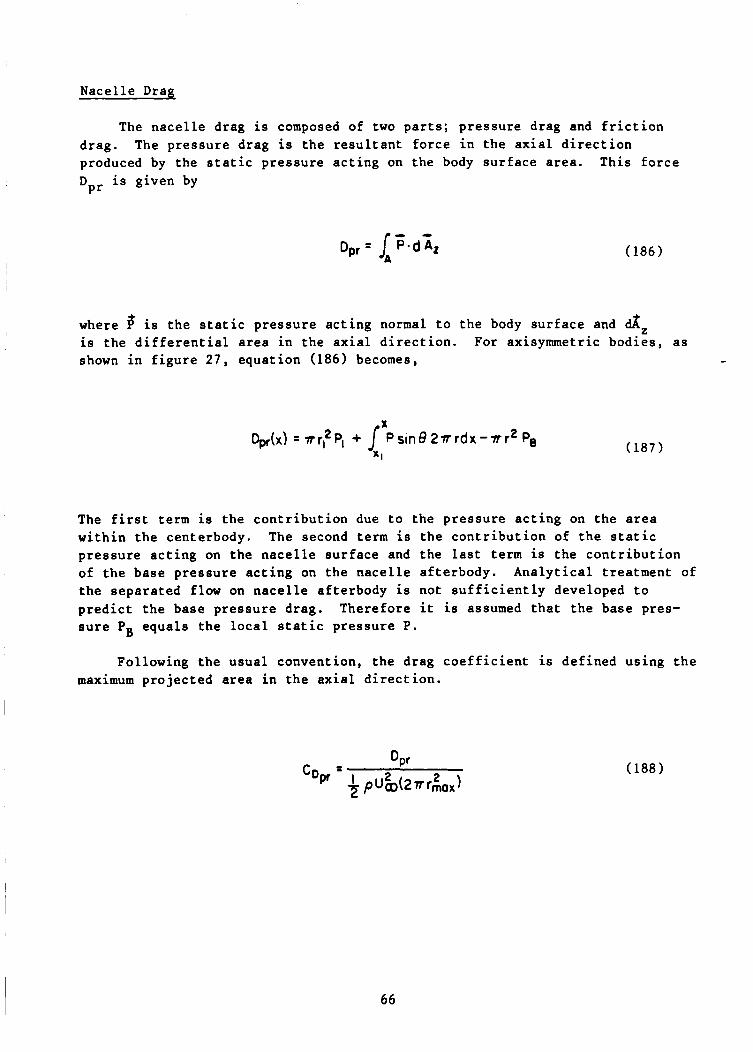
Nacelle Drag

The nacelle drag is composed of two parts; pressure drag and friction drag. produced by the static pressure acting on the body surface area. This force Dpr is given by

The pressure drag is the resultant force in the axial direction

( 1 8 6 )

I where 3 is the static pressure acting normal to the body surface and d, is the differential area in the axial direction. For axisymmetric bodies, as shown in figure 27, equation (186) becomes,

The first term is the contribution due to the pressure acting on the area within the centerbody. The second term is the contribution of the static pressure acting on the nacelle surface and the last term is the contribution of the base pressure acting on the nacelle afterbody. the separated flow on nacelle afterbody is not sufficiently developed to predict the base pressure drag. Therefore it is assumed that the base pressure PB equals the local static pressure P.

Analytical treatment of

Following the usual convention, the drag coefficient is defined using the maximum projected area in the axial direction.

66

The n a c e l l e f r i c t i o n d rag i s produced by t h e n a c e l l e boundary l a y e r . This is determined by i n t e g r a t i n g t h e a x i a l component of w a l l stress a c t i n g on t h e wetted area on t h e n a c e l l e a s shown i n f i g u r e 27.

The f r i c t i o n drag c o e f f i c i e n t is then g iven by

where t h e p ro jec t ed a r e a r a t h e r than wetted a r e a i s used t o keep i t c o n s i s t e n t with t h e d e f i n i t i o n of p re s sue drag c o e f f i c i e n t .

Numerical S o l u t i o n

With t h e r e l a t i o n s h i p between and t h e mean f low s p e c i f i e d , equa t ions (124) through (133) can be so lved by an i m p l i c i t forward marching numerical i n t e g r a t i o n scheme. These equat ions are f i r s t l i n e a r i z e d by expanding a l l dependent v a r i a b l e s i n a Taylor series expansion i n t h e marching d i r e c t i o n (81 , and terms o f 0 ( b e ) are dropped. ob ta ined us ing t h e two poin t cen tered d i f f e r e n c e scheme o f Keller ( r e f e r e n c e s 62 and 63) . and are solved by b lock f a c t o r i z a t i o n us ing t h e method of Varah ( r e f e r e n c e 64).

F i n i t e d i f f e r e n c e equat ions are t h e n

The r e s u l t i n g ma t r ix equat ions are (10 x 10) b lock t r i d i a g o n a l

This numerical s o l u t i o n is second o r d e r a c c u r a t e i n t h e n d i r e c t i o n , The b s t e p s i ze is f i r s t o r d e r i n t h e s d i r e c t i o n , and l i n e a r l y s t a b l e .

l imi t ed not by l i n e a r s t a b i l i t y c o n d i t i o n s , bu t by t h e r equ i r ed accuracy in t h e Taylor series expansion i n 8 .

67

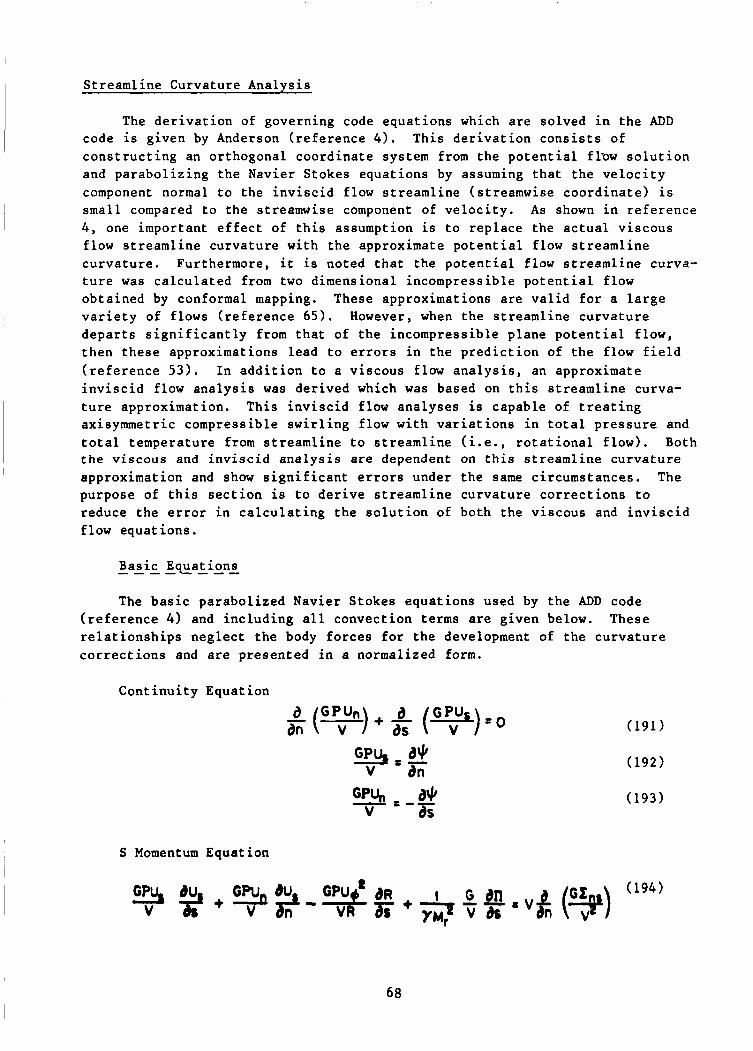
Streamline Curvature Analysis

The derivation of governing code equations which are solved in the ADD code is given by Anderson (reference 4 ) . This derivation consists of constructing an orthogonal coordinate system from the potential ftow solution and parabolizing the Navier Stokes equations by assuming that the velocity component normal to the inviscid flow streamline (streamwise coordinate) is small compared to the streamwise component of velocity. As shown in reference 4 , one important effect of this assumption is to replace the actual viscous flow streamline curvature with the approximate potential flow streamline curvature. Furthermore, it is noted that the potential flow streamline curvature was calculated from two dimensional incompressible potential flow obtained by conformal mapping. These approximations are valid for a large variety of flows (reference 6 5 ) . However, when the streamline curvature departs significantly from that of the incompressible plane potential flow, then these approximations lead to errors in the prediction of the flow field (reference 53). In addition to a viscous flow analysis, an approximate inviscid flow analysis was derived which was based on this streamline curvature approximation. This inviscid flow analyses is capable of treating axisymmetric compressible swirling flow with variations in total pressure and total temperature from streamline to streamline (i.e., rotational flow). Both the viscous and inviscid analysis are dependent on this streamline curvature approximation and show significant errors under the same circumstances. The purpose of this section is to derive streamline curvature corrections to reduce the error in calculating the solution of both the viscous and inviscid flow equations.

I

Basic Ewat ions ---- --- The basic parabolized Navier Stokes equations used by the ADD code

(reference 4 ) and including all convection terms are given below. These relationships neglect the body forces for the development of the curvature corrections and are presented in a normalized form.

Continuity Equation

S Momentum Equation

68

4 Momentum Equation

n Momentum Equation --++--

v2 as (196 1

GP% dun GPUn v as w an

Thermodynamic Relations

n = Pe

1-

(201 1

(202)

(203)

(204)

(205

(206 1

69

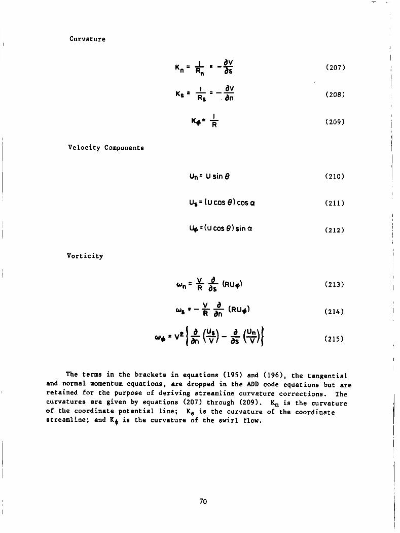
I

Curvature

av Kn an as

t L t -- I av

K s = R t = - - an

(207 1

(208 1 I

Velocity Components

Un= U sin 8

us = (u cos 8 ) cos a

w = ( U c o s B ) s i n a

Vorticity

The terms in the brackets in equations (195) and (196), the tangential

The Kn is the curvature

and normal momentum equations, are dropped in the ADD code equations but are retained for the purpose of deriving streamline curvature corrections. curvatures are given by equations (207) through (209). of the coordinate potential line; streamline; and KQ, is the curvature of the swirl flow.

K, is the curvature of the coordinate

70

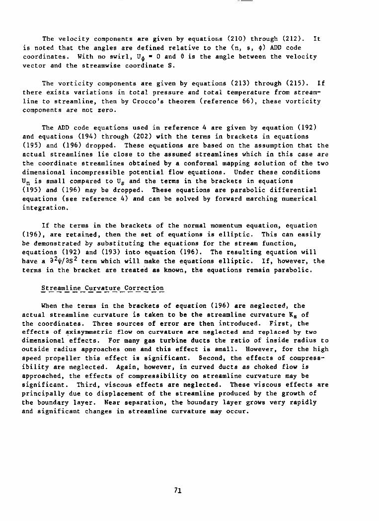
The velocity components are given by equatioris (210) through (212). It is noted that the angles are defined relative to the (n, s, $1 ADD code coordinates. vector and the streamwise coordinate S.

With no swirl, U,#, = 0 and 8 is the angle between the velocity

The vorticity components are given by equations (213) through (215). If there exists variations in total pressure and total temperature from streamline to streamline, then by Crocco's theorem (reference 661, these vorticity components are not zero.

The ADD code equations used in reference 4 are given by equation (192) and equations (194) through (202) with the terms in brackets in equations (195) and (196) dropped. These equations are based on the assumption that the actual streamlines lie close to the assumed streamlines which in this case are the coordinate streamlines obtained by a conformal mapping solution of the two dimensional incompressible potential flow equations. Under these conditions Un is small compared to Us and the terms in the brackets in equations (195) and (196) may be dropped. These equations are parabolic differential equations (see reference 4) and can be solved by forward marching numerical integration.

If the terms in the brackets of the normal momentum equation, equation (1961, are retained, then the set of equations is elliptic. This can easily be demonstrated by substituting the equations for the stream function, equations (192) and (193) into equation (196). The resulting equation will have a a 2 $ / a S 2 term which will make the equations elliptic. terms in the bracket are treated as known, the equations remain parabolic.

If, however, the

Streamline Curvature Correction ---------------- When the terms in the brackets of equation (196) are neglected, the

actual streamline curvature is taken to be the streamline curvature Ks of the coordinates. Three sources of error are then introduced. First, the effects of axisynnnetric flow on curvature are neglected and replaced by two dimensional effects. For many gas turbine ducts the ratio of inside radius to outside radius approaches one and this effect is small. However, for the high speed propeller this effect is significant. Second, the effects of compressibility are neglected. Again, however, in curved ducts as choked flow is approached, the effects of compressibility on streamline curvature may be significant. Third, viscous effects are neglected. These viscous effects are principally due to displacement of the streamline produced by the growth of the boundary layer. Near separation, the boundary layer grows very rapidly and significant changes in streamline curvature may occur.

71

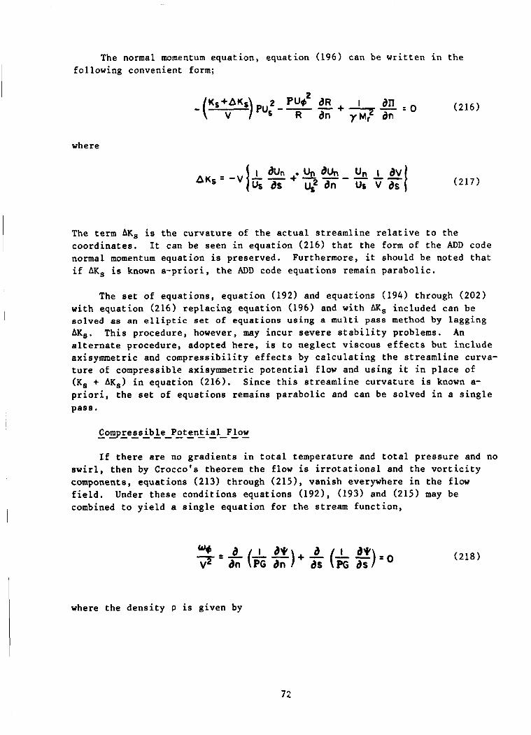
The normal momentum equation, equation (196) can be written in the following convenient form;

where

The term AKs is the curvature of the actual streamline relative to the coordinates. It can be seen in equation (216) that the form of the ADD code normal momentum equation is preserved. Furthermore, it should be noted that if AKs is known a-priori, the ADD code equations remain parabolic.

The set of equations, equation (192) and equations (194) through (202) with equation (216) replacing equation (196) and with AK, included can be solved as an elliptic set of equations using a multi pass method by lagging AKs. This procedure, however, may incur severe stability problems. An alternate procedure, adopted here, is to neglect viscous effects but include axisymmetric and compressibility effects by calculating the streamline curvature of compressible axisymetric potential flow and using it in place of (Ks + AK,) in equation (216). Since this streamline curvature is known a- priori, the set of equations remains parabolic and can be solved in a single pass.

Coyressible Potential Flow - ------------ If there are no gradients in total temperature and total pressure and no

swirl, then by Crocco's theorem the flow is irrotational and the vorticity components, equations (213) through (2151, vanish everywhere in the flow field. Under these conditions equations (1921, (193) and (215) may be combined to yield a single equation for the stream function,

where the density p is given by

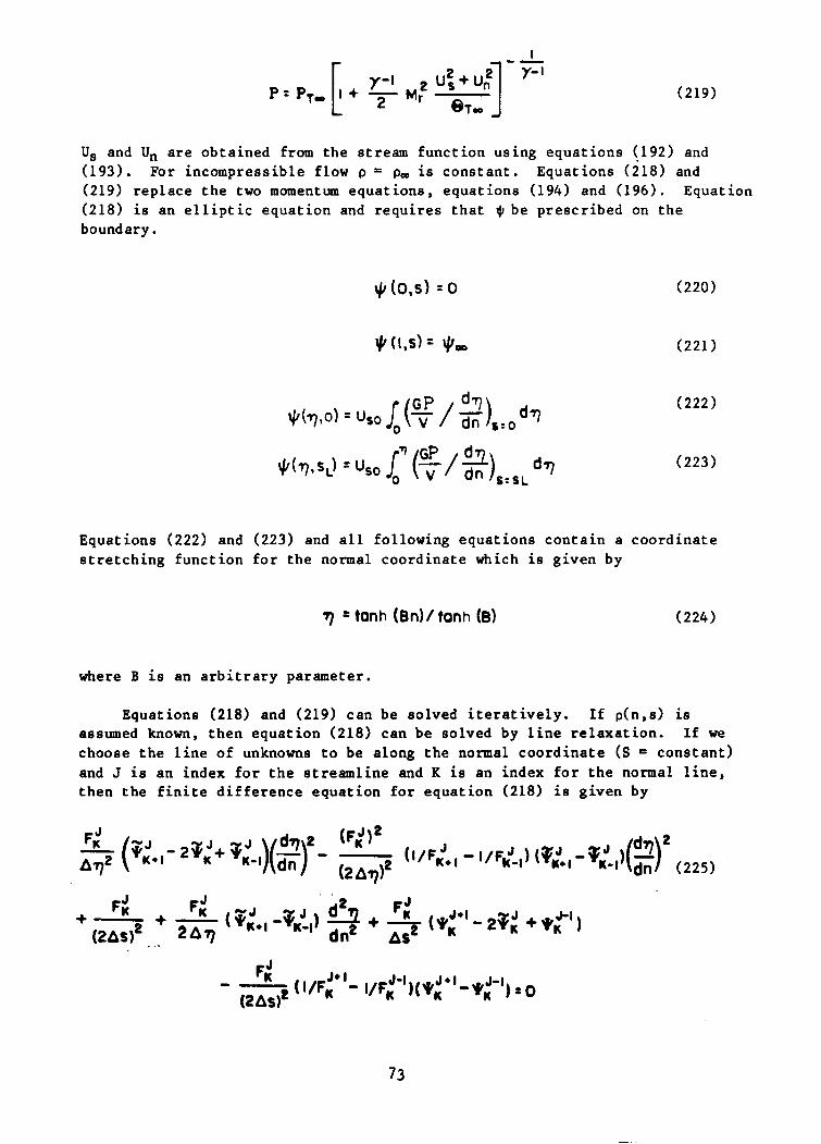
I c

Us and Un a r e obta ined from t h e stream func t ion us ing equa t ions (-192) and (193) . For incompress ib le flow p = pao is cons t an t . Equations (218) and (219) r ep lace t h e two momentum equa t ions , equa t ions (194) and (196). Equation (218) is an e l l i p t i c equa t ion and r e q u i r e s t h a t $ b e p resc r ibed on t h e boundary.

JI(OIS, = o

= \Loo

Equations (222) and (223) and a l l following equa t ions c o n t a i n a c o o r d i n a t e s t r e t c h i n g func t ion f o r t h e normal coord ina te which i s g iven by

where B is an a r b i t r a r y parameter.

Equations (218) and (219) can be solved i t e r a t i v e l y . I f p(n,s) is assumed known, then equa t ion (218) can be solved by l i n e r e l a x a t i o n . I f we choose t h e l i n e of unknowns t o be along t h e normal c o o r d i n a t e (S and J is an index f o r t h e s t r e a m l i n e and K i s an index f o r t h e normal l i n e , then t h e f i n i t e d i f f e r e n c e equa t ion f o r equa t ion (218) i s g iven by

cons t an t )

73

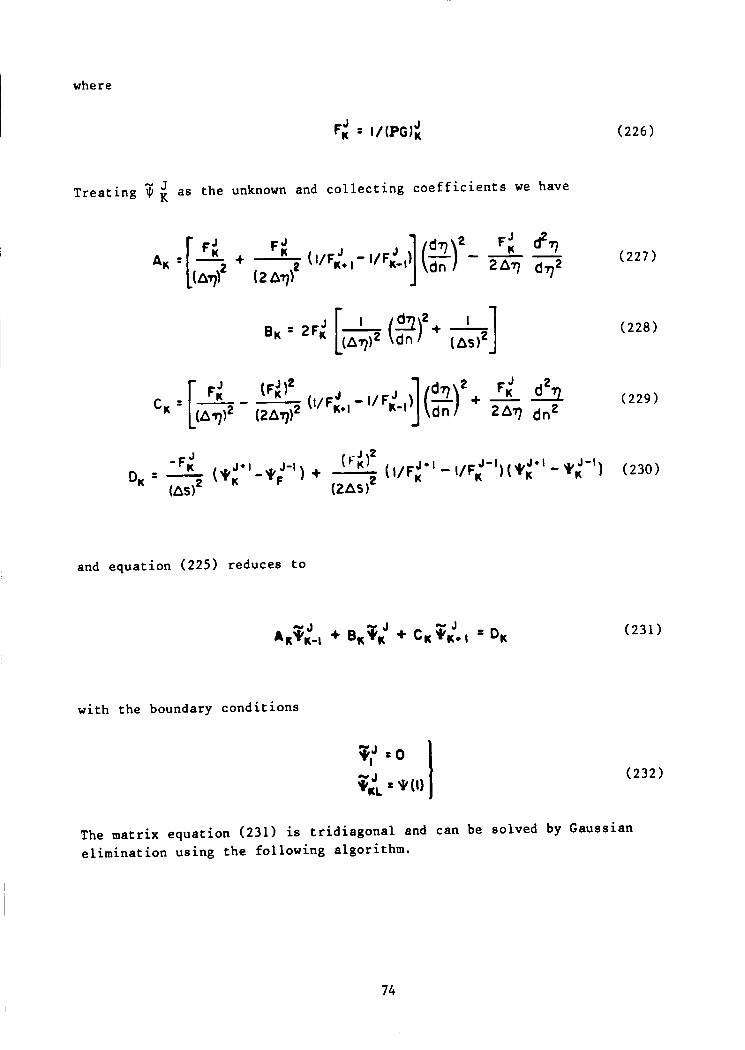
where

J Treating 5 as the unknown and collecting coefficients we have

A, = (227)

(228)

(229)

and equation (225) reduces to

with the boundary conditions

The matrix equation (231) is tridiagonal and can be solved by Gaussian elimination using the following algorithm.

74

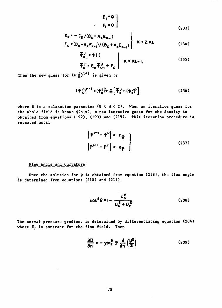
1

Then the new guess for ( J , ;Iw1 is given by

(233)

(234)

(235)

where Q is a relaxation parameter (0 < Q < 2). the whole field is known J,(n,x>, a new iterative guess for the density is obtained from equations (1921, (193) and (219). This iteration procedure is repeated until

When an iterative guess for

Flow Angle and Curvature ------------ Once the solution for J, is obtained from equation (2181, the flow angle

is determined from equations (210) and (211).

4 u t + u t

c 0 8 8 = I - (238)

The normal pressure gradient is determined by differentiating equation (204) where IIT is constant for the flow field. Then

75

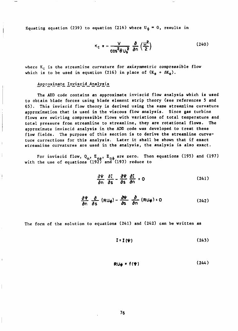
Equating equation (239) to equation (216) where U+ = 0, results in

I v K C t -

cos28u: an ( 240 1

where Kc is the streamline curvature for axisymmetric compressible flow which is to be used in equation (216) in place of (K, + AKs).

Aplroximate Inviscid Ana9EiE - - - - - - - - - - - The ADD code contains an approximate inviscid flow analysis which is used

to obtain blade forces using blade element strip theory (see references 5 and 65). This inviscid flow theory is derived using the same streamline curvature approximation that is used in the viscous flow analysis. flows are swirling compressible flows with variations of total temperature and total pressure from streamline to streamline, they are rotational flows. The approximate inviscid analysis in the ADD code was developed to treat these flow fields. ture corrections for this analysis. Later it shall be shown that if exact streamline curvatures are used in the analysis, the analysis is also exact.

Since gas turbine I

The purpose of this section is to derive the streamline curva-

, For inviscid flow, Qn, En , En+ are zero. Then equations (195) and (197) with the use of equations (1927 and (193) reduce to

The form of the solution to equations (241) and (242) can be written as

76

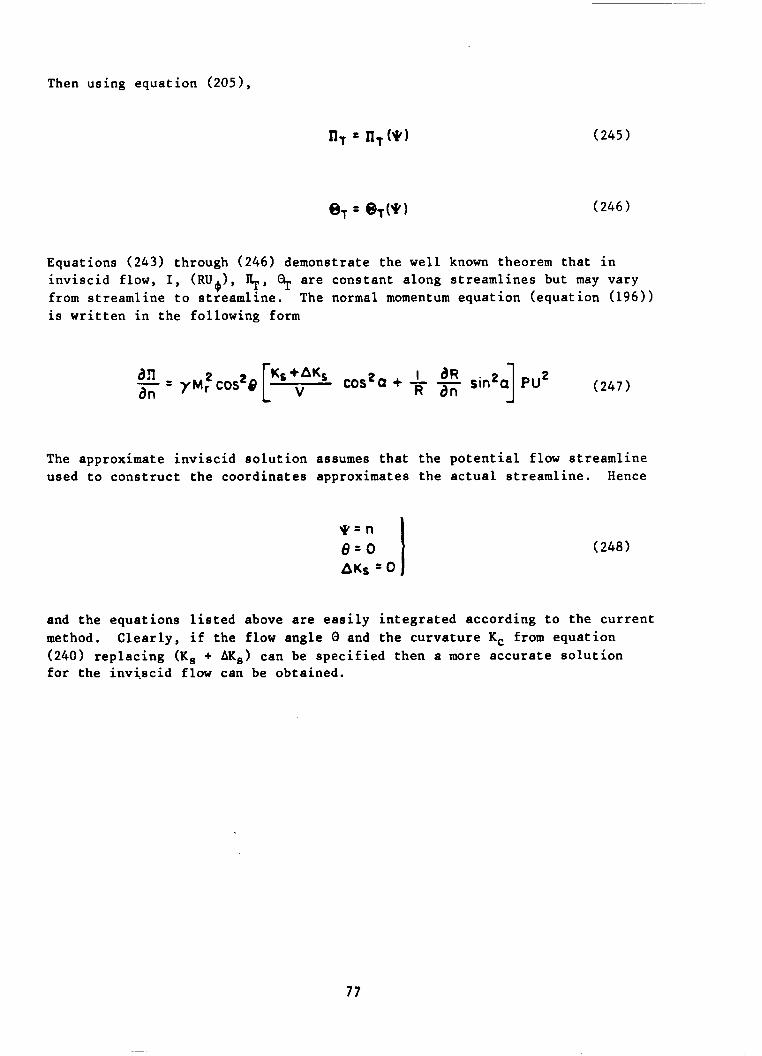
Then using equation (2051,

Equations (243) through (246) demonstrate the well known theorem that in inviscid flow, I, (RIJ+) , I$,, Q1. are constant along streamlines but may vary from streamline to streamline. is written in the following form

The normal momentum equation (equation (196))

1 (247) COS a + - - sin2q pu2 an 2 Ks +AK, 2 I dR R a n a n - = yM, Cos2@

The approximate inviscid solution assumes that the potential flow streamline used to construct the coordinates approximates the actual streamline. Hence

y = n e = o 1 A K ~ = O

(248 1

and the equations listed above are easily integrated according to the current method. Clearly, if the flow angle 8 and the curvature K, from equation (240) replacing (Ks + AKs) can be specified then a more accurate solution for the invi-acid flow can be obtained.

77

COUPLING PROCEDURE

Assumptions Affecting the Coupling

As noted in the Introduction, the coupling of the two separate procedures for the nacelle and propeller portions of the analysis requires the transfer of pertinent data affecting the respective solution procedures of the analysis. The ability to use this solution technique to obtain the combined propeller-nacelle performance prediction is based upon the following major assumptions related to the coupling process which are noted below.

As was noted in the technical approach for the propeller solution procedure, the flow field is steady with respect to the propeller blades; however, this is not true when the point of reference is the nacelle wall boundary. an assumption concerning the propeller's influence must be made in order to use the nacelle analysis and to avoid the necessity to calculate the local time varying induced flow field about the nacelle due to the rotating propeller and wake. The assumption is made that the inclusion of the effects of the propeller on the nacelle and surrounding flow field can be handled in a time-averaged manner by including only the addition of the local blade forces at the blade row locations and that this model will adequately approximate on a time-averaged basis the effects of the combined blade and trsiling wake system in the flow, to predict the flow field about the combined propeller- nacelle configuration.

Because the nacelle analysis does assume time-averaged properties,

To calculate the forces on the propeller blades it is necessary to assume that the nacelle flow field solution is representative of the actual flow field. Since this is a basic assumption of the nacelle portion of the combined analysis, no further explanations are necessary concerning the nacelle portion of the analysis in terms of the coupling procedure. assumptions concerning the influence of the nacelle on the wake geometry were described in the section entitled: Nacelle Influence on the Wake Geometry, and are not repeated here.

The

PRECRDING PAGE BLANK NOT F I L W

79

Description of the Combined Analysis Solution Procedure

To obtain the combined propeller-nacelle performance solution, the interfacing of the propeller and nacelle solution procedures requires the transfer of data between the two portions of the analysis. In the combined-analysis, the propeller portion requires that the local inflow conditions (velocity, density and speed of sound) at the blade row(s) be specified and that the wake geometry be corrected for the presence of the nacelle, if so desired. The nacelle portion requires that the lifting line geometry and local blade forces (radial, tangential, axial) per unit length be specified for the propeller blade row(s). Figure 28 is a simplified flow diagram of the combined solution procedure with the required transfer of data noted, as developed for this application. The major tasks performed in the analysis associated with the pertinent features of the combined analysis are also shown in this flow diagram.

The structure of the solution procedure is shown in the diagram. Within the analysis there are two ways in which the combined analysis can be used. First, the program can be run with only the inviscid flow field calculated to define the inflow and wake perturbations for the propeller portion of the analysis to obtain the combined propeller and nacelle performance; however, the blade forces are not included in the inviscid nacelle solution. This may be desirable for cost considerations if it is shown that the viscous solution does not significantly change the propeller performance predictions as compared with the inviscid propeller performance predictions, and, if the inclusion of the blade force's influence on the nacelle performance is not desired. Second, if the viscous solution is desired, the analysis can also be made to cycle through the viscous portion a selected number of times. This mode will include the blade force's influence on the nacelle performance. The selection of the number of cycles required to obtain compatible solutions must be determined from the user's experience. Based on the experience gained in the development of the computer analysis, it is believed that generally only one cycle will be required. However, this assumption remains to be proven in actual practice. It should also be noted that for the viscous solution's influence at the blade, it is not currently possible to separate, from the viscous velocity field solution, the portion of the inflow due to the addition of the blade forces. To resolve this problem, the calculation of the flow field due to the nacelle at the blade row is performed at the blade leading edge in the viscous solution procedure. This approach removes the blade force's influence on the flow field at the propeller because of the parabolic nature of the problem. That is, the inclusion of the blade forces, distri- buted over the blade surface, is not felt at the leading edge of the propeller blades, only downstream of this location.

INITIAL APPLICATION OF THE ANALYSIS

The initial application of the analysis was performed under Contract NAS3-20961 and was limited to a single propeller-nacelle configuration and test condition. The results obtained from this application indicated that the inflow velocities due to the nacelle body were incorrectly predicted at the blade row. This finding was verified by the use of an alternate nacelle analysis to predict the velocity profile at the blade row location. In addition to this problem, the use of the computer program requires the selection of various propeller aerodynamic modeling features which can significantly affect the performance predictions. As a result, Contract NAS3-22142 was established to refine and modify the analysis to remove known problems and to expand the scope of the application of the analysis to include different propeller nacelle configurations, test conditions, and modeling features. Following this effort additional applications of the analysis have been made under Contract NAS3-22257 to configurations and operating conditions for which test data is available for comparison.

In general, the results of the initial application of the analysis will not be reported herein because of the limited nature of that study. It is sufficient to note that this single application led to the more expanded application and refinement effort for the contracts noted above. The results of this expanded application are reported below. This study includes a comprehensive investigation of the effects of the propeller aerodynamic modeling features, the sensitivity of results to the airfoil characteristics defined for the same airfoil section from different sources, the application of the analysis to different operating conditions, and the application of the analysis to different propeller-nacelle configurations which include single and coaxial geometries.

NACELLE FLOW FIELD PREDICTIONS

The combined analysis requires that both the flow field around the nacelle body and the blade loading solution be predicted with reasonable accuracy. Both solutions are predicted based on the super-position of the individual solutions in a cyclic manner. The refinements to the original axisymmetric duct flow field solver (ADD Code, references 4 and 5 ) to treat axisymmetric nacelle configurations with or without wind tunnel wall influence (including tunnel wall bleed) have resulted in an analysis (PANPER) capable of treating a wide range of high speed propeller configurations when combined with the propeller blade loading analysis. The verification of the ability of the analysis to predict the flow field perturbations around the nacelle for these high speed conditions was performed by comparing predictions for an isolated nacelle at Mach Numbers of .2, .7, and .8 with the predictions obtained using an established transonic, inviscid flow field solver for axisymmetric bodies (RAXBOD, references 67 and 68). The results of this comparison are presented for the .8 Mach Number condition. The results at .2 and . 7 Mach number will not be presented, but are similar in the degree of correlation.

In figure 29, the predicted nacelle wall pressure distributions for the SR-3 Nacelle design at .8 Mach Number are shown for both the PANPER and the RAXBOD codes. An example of this propeller blade planform is shown in figure 30 for illustration purposes. Superimposed on figure 29 is the corresponding nacelle profile and the approximate location of the blade lifting line. The prediction for the pressure distribution using the PANPER analysis differs from the RAXBOD prediction near the nose of the nacelle. This is due to the use of an optional smoothing process in the PANPER analysis applied to the nacelle profile coordinates resulting in slightly different local profile coordinates. Further downstream, past the blade row in the region of the high curvature of the nacelle profile, the predicted solutions also exhibit some differences. The RAXBOD analysis predicts a lower pressure distribution corresponding to a region of transonic flow. The PANPER analysis, which is not a transonic flow analysis, clearly does not predict the same pressure distribution. It should be noted that the PANPER analysis yielded nearly identical results for both the inviscid and viscous pressure distributions for the other lower Mach number conditions. These comparisons indicate that the general character and level of the nacelle wall pressure distributions are reasonably predicted, although regions of supersonic flow are not correctly modeled. However, this discrepancy is probably not significant for propeller performance predictions in the region of the blade lifting line location as will be shown in the next section.

83

During the course of this investigation test measurement data for the flow field upstream of a non-lifting propeller, obtained in the NASA Lewis Research Center test facilities, was made available to UTRC and has been . presented in reference 69. The results of applying the nacelle code to these test results are included herein as an additional example of the code's predictive capability. This study also illustrates the need to include the effect of blade thickness in the nacelle flow field solution procedure when using the analysis to predict the flow field upstream of the blade row. The condition investigated was at . 8 Mach Number for the non-lifting SR-3 propeller/nacelle configuration. The flow measurements were obtained using laser velocimetry techniques at an axial position .09 propeller radii upstream of the propeller blade row. Three different nacelle flow field solutions were obtained to demonstrate the effect of different streamline curvature models and the presence of the blades in the solution procedure. The results in figure 31 present the measured and predicted Mach Number distributions along the blade lifting line location for this condition. The results of the different streamline curvature models, without blade thickness, illustrate the improvement in the predictive capability of the nacelle code when the two- dimensional streamline curvature model of the original analysis was modified to an axisymmetric streamline curvature model for propeller application. The inclusion of the blade thickness in the axisymmetric streamline curvature model further improves the flow field predictions near the high solidity region of the propeller blades where the presence of the blade should.be most strongly felt. The discrepancy in the overall level of the flow field (Mach Number) away from the nacelle wall may indicate that the actual condition tested is not a true 0 . 8 Mach number condition. If the analysis were run to match the implied freestream Mach Number of the test results, the correlation would be excellent over most of the range of radial positions measured. Near the nacelle wall, the results would differ slightly. This difference could be due to either the numerical model or a slight difference in the location of the measured data compared with the position used in the analysis. Another possible reason for the difference is that the SR-3 propeller is never truly non-lifting in a local sense. The blade's integrated lift may be zero, but the local blade loading can be non-zero. Thus, there could be the effect of a local lift induced flow field in the test results. The analysis was run without the blade forces, and thus there are no lift induced velocities included in the predictions.

84

The use of the nacelle induced flow field at the propeller blade as predicted by the nacelle portion of the PANPER analysis requires that the locations along the blade at which the velocity components are calculated be specified. stream conditions requires that the angle of attack at the wing quarter-chordline be defined using the freestream velocity and the induced velocity. The propeller lifting line solution is an extension of this concept to the propeller environment which includes the rotational and nacelle induced velocity fields. Near the nacelle, the nacelle induced flow field varies in the radial and axial directions (axisymmetric assumption). Thus, the nacelle induced flow field used in the propeller portion of the analysis is affected by the selection of the location (blade quarter-chordline, leading edge, etc.) at which this information is calculated. The selection of these locations has not yet been clearly defined. In figure 32, the axial component of the nacelle flow field, as predicted using the nacelle portion of the PANPER analysis, is presented along the blade leading edge and the blade quarter- chordline with and without the inclusion of the blade thickness in the streamline curvature model. The results indicate that the axial velocity is relatively insensitive to the selection of the prediction location for the solution obtained neglecting the blade thickness influence in the streamline curvature model. However, when the blade thickness is included in the solution procedure, the axial velocity component shows a strong sensitivity to the selection of the,prediction location. It should be noted that the radial velocity component does not exhibit this strong sensitivity as shown in figure 33.

Traditional Prandtl lifting line theory under uniform free-

The sensitivity of the axial velocity to the selected prediction location introduces an additional uncertainty in the use of the analysis. Since the propeller portion of the analysis already recognizes the high solidity regions of the blade near the hub walls through the use of the cascade characteristics, the use of the blade thickness influence in the prediction of the nacelle induced flow field solution is actually "double accounting" for the blade thickness. Thus, for propeller performance predictions, the most appropriate way of using the analysis may be to either; include the blade thickness in the nacelle induced flow field solution without using cascade characteristics in the lifting-line propeller solution, or conversely, use the cascade characteristics in the propeller solution without the blade thickness influence in the nacelle flow field solution. However, for the first method the selection of the prediction location (leading edge, quarter chordline, trailing edge) for the nacelle induced velocities as used in the propeller analysis has not been adequately investigated. As a result, the analysis is generally run for propeller performance predictions using the second method of neglecting the blade thickness influence in the nacelle induced flow field. For nacelle induced flow field predictions away from the propeller disk, the nacelle analysis should be run including the effects of blade thickness as was done for the results presented in figure 31. This is necessary because the lifting-line models do not account for thickness in the propeller induced field.

85

SINGLE PROPELLER PERFORMANCE PREDICTIONS

Aerodynamic Modeling Features

The development of the propeller portion of this analysis is'based on the application of methodologies which have been extended to the limits of their operational applicability to attempt to provide a useful, numerically efficient performance analysis. To provide this type of analysis tool using the incompressible lifting line model required the inclusion of many different aerodynamic modeling features. These features attempt to include in a rational manner the effects of compressibility on the propeller tip loading, the effects of compressibility on the propeller wake induced velocity field, the influence of the nacelle flow field, the effects of the high solidity inboard blade sections using cascade data or corrections to isolated airfoil data for the cascade influence, the effects of highly swept blades, and the selection of different sources of isolated airfoil and cascade characteristics. This large number of modeling features has resulted in an even larger number of combinations of these features which can be used when predicting the propeller performance. In addition, these features do not address the question concerning the inclusion of the blade thickness influence in the nacelle flow field solution procedure noted earlier. Obviously many combinations are unrealistic, however there are still a large number of realistic combinations which can be used. This investigation has attempted to define a reasonable combination of these features by applying the analysis to different propeller-nacelle configurations and operating conditions to study the results, examine the sensitivities to modeling options and compare the predictions with test data where available. These comparisons are presented to provide some useful insight into the best selection of these modeling features.

Through out this report the terms net and apparent efficiency are used. For clarity they are defined herein. in the tunnel by the force balance for the total system installation. In a simplistic sense this is the total of the propeller forces and nacelle body forces. propeller forces generated in the presence of the nacelle. of the actual body is to reduce the efficiency, the apparent efficiency is usually higher than the net by some small correction (An).

The net efficiency (n) is that measured

The apparent efficiency (nA) is the component due only to the Since the effect

PRECBDING PAGE BLANK NOT FILMED

87

The analysis can only predict the apparent efficiency since the nacelle body force predictions are valid only up to the termination of the body model or the separation point. Since separation usually occurs for the afterbodies used for these studies, the model was truncated reasonably far downstream from the blade row, but did not have closure on the geometry. Estimates for the back pressure can be made, but they are not of sufficient accuracy for this study. For comparisons without test results, the apparent efficiencies are used. In this report, the choice of the use of apparent or net efficiencies for comparison with test data was based on the effort required to adjust either the data or the predictions. Where the amount of test data was small compared to the number or prediction cases run, the data was correct to apparent efficiency. For the cases where the amount of data was larger, the predicted efficiencies were corrected to net values. These corrections were supplied by NASA.

The results presented herein start with the application of the analysis to selected propeller and nacelle configurations to compare the different aerodynamic modeling features. The influence of the nacelle on the solution is neglected for these preliminary applications. The intention is to define and illustrate the sensitivity of the propeller performance predictions to the modeling features. data are available. For this application the effects of the different modeling features are again studied with the number of features limited in scope based on the first series of applications. However, because test data are available, the nacelle influence is included for this study. And finally,. the analysis is applied to configurations in selected 'wind tunnel facilities to identify any potential problems in the use of the different facilities with the model scaling selected.

The analysis is then applied to conditions for which test

Single Propeller-Nacelle Configurations

Fundamentally the single propeller-nacelle configurations studied represent variations in blade design and nacelle shape. The variation in blade design include blade sweep, taper, twist, solidity, and thickness changes for the different blade geometries. The nacelle geometries studied were either the area ruled or conical shaped profiles. These nacelle profiles are shown in figure 3 4 . The propeller geometries were the NASA designated SR- 2, SR-1, SR-lM, and SR-3 designs; representing respectively, straight to moderately swept blades (0, 3 0 , and 45 degrees). SR-1 and the SR-1M designs is the blade tip twist and section camber. The airfoil sections were the NACA Series 1 6 , transitioning to series 65 near the blade root. are presented in graphical form in figures 35 to 3 7 . ehown earlier in figure 30 for these designs.

The difference between the

The blade design characteristics €or each propeller configuration The plan forms were

88

Single Propeller-Nacelle Operating Conditions

The range of operating conditions studied was based on the range of early unpublished test data provided by NASA. The range in free-stream Mach number was from 0.6 to 0.8. For the initial studies, which investigated.sensitivities to the modeling options, the variations in rpm at a fixed power loading (constant power) provided advance ratio variations in the range of 2.6 to 3.2. For the performance map predictions shown later, the advance ratio variations were in the range of 2.5 to 4.5 with blade angle variations in the range of 58 to 63 degrees depending on the propeller configurations and free-stream Mach number conditions (0.6 and 0.8). from near windmilling conditions to as high as 3.0 depending on the combination of conditions. The design condition, when referenced herein, corresponds to an advance ratio fo 3.07 with a power coefficient of 1.69.

The range in power coefficients studied has

To help in determining when operating conditions represent supersonic tip speeds, the following relationship can be.used to find the advance ratio which corresponds to a tip Mach number of 1.0.

For the 0.6 free-stream Mach number condition there was no advance ratio condition studied which had supersonic tips. At the 0.7 Mach number condition, supersonic tip conditions existed for advance ratios less than 3.079. However, at the design point advance ratio (3.07) for this Mach number, the fraction of blade radius which experiences supersonic flow is very small (0.003R). For the 0.8 Mach number condition all advance ratio conditions less than 4.189 had supersonic tip Mach numbers. At the design point the outer 25 percent of the blade is operating in supersonic flow.

Effect Of Compressible Tip Loss Models

The analysis currently has four compressible flow tip loss models available along with the non-tip loss model. These models were described in an earlier technical section, but for convenience they will be briefly described here. The first model is the Evvard model (tabulated solutions) which is based on fixed wing, rectangular tipped geometries applied to the non-rectangular geometries of the high speed propeller designs. The second model is an exact analytical integration of the relations used in conical flow

89

theory for the rectangular wing tip. In theory this model is identical to the Evvard model which is available in tabular form, however there are small differences in practice. The third model is based on conical flow theory for swept wings assumed to be operating at a free-stream Mach number equal to 'the propeller tip Mach number. where the tip loss correction is further scaled using the ratio of the Prandtl Glauert compressibility corrections based on the propeller's local section and tip. Only the tabulated Evvard and the swept conical flow models were studied in depth and Mach numbers compared with the non-tip loss model results. The analysis was applied using the SR-1, SR-2, and SR-3 propellers with the area ruled spinner and nacelle geometry at; (1) the design advance ratio for a variation in free-stream Mach number at the design power coefficient, (2) the design advance ratio with a variation in the design power coefficient for a fixed Mach number, and (3) the design power coefficient for a variation of the advance ratio at a fixed Mach number. For some of the conditions investigated using the swept conical flow tip loss models, solutions were not obtained because the combination of blade geometry and operating condition violated assumptions used in the model. For this study, the analysis was applied using the cascade data correlations from reference 40 and the cascade correction based on flat plate theory was applied to the isolated airfoil data of Manoni over the blade transition region. The compressible wake model was used for all of the above cases. In addition, the influence of the nacelle w a s neglected for this study and thus the predicted results should not be considered indicative of the actual propeller performance capabilities. The results are presented separately in figures 38 to 40 for each propeller configuration. In these figures, the propeller efficiency is plotted on a greatly expanded scale as a function of the free-stream Mach number to illustrate the differences in the predictions using the various tip loss models.

The fourth model is a variation of th-is model

.

The results of the application of the analysis to the unswept propeller blade design (SR-2) are presented in figure 38. At the 0.7 Mach number (tip Mach number 1.0051, all tip loss models appear to function in the analysis, but the results are identical. This is because the supersonic region is too small (0.3 percent of radian) relative to the size of the lifting line segments along the blade and does not activate any of the models. The swept conical flow tip loss models are not used at the 0.8 Mach number for this propeller geometry because the assumptions used to develop the model are violated; the trailing edge of the blade must be supersonic. The effect of the Evvard tip loss model for all of the conditions at this Mach number is to reduce the propeller efficiency for a specified power level. When the analysis was run at a specified blade pitch the same effect was noted, although these results are not presented.

90

For the SR-1 propeller, a 30 degree swept blade design, the results of the application of the different tip loss models are shown in figure 39. Again, the lower Mach number condition (0.7) does not activate any of the models and the swept conical flow tip loss models can not be applied for this design at the 0.8 Mach number conditions. The Evvard model again results in the reduced efficiency compared with the non-tip loss model.

For the SR-3 propeller, a 45 degree swept blade design, the results of the application of the different tip loss models are presented in figure 40. At the 0.7 Mach number the swept conical flow models are again not applicable because the supersonic trailing edge requirement of the model is not met. At this Mach number the difference between the non-tip loss and the Evvard tip loss model results are small. The results for the application at 0.8 Mach number vary depending on the loading condition and advance ratio. The reduced loading condition (Cp'1.5) at the 3.07 advance ratio exhibits no significant difference between the swept conical flow tip loss models and the non-tip loss model while the use of the Evvard model results in a reduced efficiency prediction. At the design loading condition (Cp'1.7) for this advance ratio the swept conical flow tip loss models do result in a difference in the predicted efficiency at the 0.8 Mach number. The conical flow model, with the variable Mach number distribution scaling, results in relatively little effect on the performance. For the lower advance ratio case at this Mach number the use of the conical flow models results in reduced efficiency, and both models yield about the same 'level of reduction. For all cases at this Mach number the Evvard model results in reduced efficiencies.

As a result of this study the decision was made to only use the Evvard tip loss model in the applications to follow. This decision was made because the conical flow model is sensitive to propeller trailing edge geometry and Mach number as evidenced in the above results. This makes it unacceptable for general application. This selection of the Evvard model is not meant to imply that it is better than the swept conical flow tip loss models, but that as implemented, the conical flow tip loss model is not reliable as an investiga- tive tool for all of the geometries studied in this investigation.

Effect of Cascade Models

The modeling of the propeller blade lift and drag characteristics is a critical aspect of the propeller portion of the analysis. predictions can be no better than the lift and drag characteristic data used in the analysis. Within the analysis the inboard blade regions (NACA series 65 airfoil sections) operate at large chord-to-gap ratios for the high speed propeller designs under investigation by NASA. istics do not represent these cascade type blade sections. Two different

The performance

Isolated airfoil character-

91

sources of cascade data have been provided in the analysis to model these blade section lift and drag characteristics. Both models are correlations, the first based on the NASA method of reference 4 0 , the second on the method by Mellor (references 49 to 51). which can be applied to isolated airfoil data based on either flat plate cascades or the Mellor correlation.

In addition the analysis has corrections

To study the influence of the cascade data on the performance predictions, the analysis was applied to the SR-1 propeller geometry using both of the cascade correlation models at the 0.8 Mach number condition for a variation in the advance ratio with a fixed blade pitch angle (60.2 deg.). For both cascade correlations used in the inboard regions, the flat plate cascade correction was used to correct the isolated airfoil characteristics along the blade transition region to attempt to model the airfoil characteristics in this region. In addition, a case was run with the isolated airfoil characteristics in this region corrected based on the Mellor correlation. (The inboard and transition regions are shown in figures 35 through 37.) case used the Mellor correlation model, resulting in three different cascade characteristic models for comparative purposes. The variation in rpm represents the range of advance ratio from near 3.0 to windmill at a fixed Mach number. Again, no nacelle influence was included for this study. The predicted propeller efficiency, power coefficient, and thrust coefficient are presented respectively in figures 41 to 43 for these conditions. The plot of efficiency versus propeller rpm (figure 41) indicates a maximum difference between the predictions for the three cascade models of about 2.5 points in efficiency except at the lowest rpm studied. difference in the predicted efficiencies is quite significant because the propeller is essentially developing zero power as shown in figure 42. outboard regions of the blades are so lightly loaded in relation to the inboard regions that differences in the inboard cascade data result in very significant differences in efficiency. For the more highly loaded conditions near the design advance ratio the outboard sections carry most of the airloading and thus the differences in the cascade data on the inboard regions do not have as significant of an effect. At these higher rpm conditions (lower advance ratio) the results obtained using the different cascade models do not show a consistent behavior in terms of the differences in predicted efficiencies for the variation in rpm; except that the efficiencies obtained using the NASA correlation model are always the highest or equal to the others. just under 1.0 point. The predicted power coefficients using these different models are shown in figure 42 to illustrate the windmill effect as the propeller rpm is reduced. The variation of the power coefficient with propeller rpm is more consistent than the efficiency was. For completeness, figure 43 shows the variation of the thrust coefficient with rpm for these different cascade models. Note that at the windmill condition the propeller is creating a drag force.

This

At this windmill condition the

The

Over this rpm region the average variation in predicted efficiency is

92

Effect Of Transition Region Interpolation Model

The transition region on the propeller blade represents the change from the NASA 65 Series airfoil sections on the inboard region of the blades to the NASA 16 Series airfoil sections on the outboard region. The analysis can currently model the airfoil characteristics in this transition region by two methods. The first method assumes that the airfoil characteristics in the transition region can be modeled by using the isolated NASA 16 Series airfoil characteristics scaled by an analytic function based on either flat plate cascade theory or the Mellor correlation to incorporate the cascade influence as a function of the local gap-to-chord ratio. Thus with this model the cascade influence diminishes concurrently with the transition to the outboard section characteristics. However, this model ignores the fact that the airfoil section in this region is neither a 16 or 65 NACA series, thus any cascade correction to the isolated 6 series data is not a true representation. The second method attempts to rectify this deficiency. It is based on an interpolation function which uses the inboard cascade data and the outboard isolated airfoil data as end point conditions to provide a functional relationship between spanwise location (gap-to-chord ratio) and section airfoil characteristics. In the analysis the behavior of the interpolation function can be varied via input of the exponent on the gap-to-chord ratio as noted in an earlier section of this report. The sensitivity of the propeller performance predictions to the modeling of the transition region characteristics is also shown in figures 41 to 4 3 . In figure 41 from the previous section, the predicted propeller efficiency is presented as a function of advance ratio for the SR-1 propeller design using different cascade correlations along with a variation in the transition region model. The variation in the transition region model is shown between the flat plate and Mellor model correction to the isolated airfoil characteristics using the Mellor cascade correlation for the inboard cascade data. The two different correction models result in relatively small differences in the predicted efficiencies, except at the windmill condition. Near the design advance ratio the difference is about two points in efficiency. Figure 44 shows the effect of applying the interpolation function to the SR-1, SR-2, and SR-3 propeller designs at design point. For this study, two different exponent values were used for both the NASA and Mellor cascade correlations. For comparative purposes, the flat plate cascade correction to the isolated airfoil characteristics was also included. As was the case for the previous studies, the nacelle influence was neglected. Comparing the results obtained using the various transition region models holding all other variables fixed indicates that the differences between the models are small, a maximum of about 2 points in efficiency. Further comparison of only the interpolation model results for the two different exponents' in the same manner shows an even smaller difference on the predicted efficiencies. isolated airfoil- data with the interpolation function in the transition region

The effect of replacing the cascade correction to

93

varies for the different propeller designs. The effect on the SR-1 is negligible, the efficiency is increased for the SR-2 using the interpolation model, and the efficiency is reduced or does not change for the SR-3 when the interpolation model is used. To demonstrate the sensitivity of the interpolation function model to the exponent used in the model the exponent was varied from 1.0 to 2.0. This variation resulted in an inconsistent behavior with increasing exponent for the different propeller designs as shown in figure 44. Generally, it appears that the use of the interpolation model in place of the correction model will increase the predicted efficiencies a small amount.

Effect of Viscous Nacelle Induced Inflow

An initial application of the analysis was performed using the SR-3 propeller/nacelle configuration to provide a performance map of propeller efficiency versus propeller rotational speed for selected blade angles at a 0.8 Mach number condition. inviscid and viscous nacelle induced influence in the solution procedure for three different blade angles at the 8440 rpm condition. The differences between the results obtained using the inviscid or viscous nacelle induced inflow are so small for the conditions studied that they are not worth presenting. As a result, the need to include the viscous nacelle induced inflow solution in the prediction of high speed propeller designs such as the SR-3 at design flight conditions does not appear to be warranted and in general it is not used in the studies to follow.

The predictions were obtained using both the

Effect of Centrifugal Blade Twist

After these SR-3 cases had been run, the SR-3 propeller design was found to have a measurable steady-state torsional deflection due to centrifugal effects. The measured deflections were for the 8440 rpm condition and are presented in figure 45 in the form of a comparison between the aerodynamic blade angle distribution with and without the centrifugal effect. of this finding, the cases were rerun with the measured torsional deflections included in the analysis. In addition, the other rpm conditions were run including the measured torsional deflections scaled by the square of the ratio of the actual rpm to the reference 8440 rpm. are presented in figure 46. most of the effort had been directed towards the SR-3 configuration, but not all combinations of modeling features had been studied. combination of modeling’features used to obtain the results presented in figure 46 are not necessarily the most appropriate. used for this study was the AIR24 (NACA data) without cascade data and a tip loss model, with the compressible wake model. From the results presented in

As a result

The results of this application At the time of the performance of this activity,

And as a result, the

The actual combination

94

figure 46 it is evident that the effect of including torsional deflections due to dynamic or aerodynamic effects can significantly alter the performance predictions. degree in the working sections of the blade for the SR-3 propeller resulted in an increase in the predicted efficiencies of 2.5 to 3 . 0 points. For all studies presented hereafter, this torsional deflection is included for the SR- 3 configuration. For the other configurations the effect is not known, but it is assumed to be small due to the severe swept angles.

The inclusion of the measured torsional deflections of over one

Comparison With Data

In the previous sections the results of applying the analysis with different aerodynamic modeling features was presented. From these studies a selected combination of modeling features were chosen for further investigation and comparison with test data. NASA Lewis Research Center and was obtained in the NASA Lewis Research Center's test facilities. nacelle's induced influence from both the inviscid and viscous solutions in the propeller performance portion of the'analysis. run on the NASA Lewis Research Center's Univac computer system.

The unpublished test data was provided by

Initially the analysis was run including the

These early cases were

As noted earlier, the results from these cases supported two major conclusions concerning the use of the analysis made during the early application and code development work. First, the use of either the inviscid or viscous flow solution resulted in essentially identical propeller performance solutions for the high speed conditions investigated. This result is not surprising in view of the assumption made in the nacelle flow field solution; that the flow field away from the body surface can be characterized by the inviscid compressible flow solution. propeller blade is operating in this region, the small differences in the l oca l flow f i e l d near the nace l le surface due to viscous e f f e c t s have very little effect in the propeller performance solution. Second, the need to cycle between the nacelle and propeller solution portions of the analysis is unnecessary for the high speed conditions studied. Again, this result is not surprising since the effect of the propeller for the conditions being studied is to induce an incremental increase in the flow around the nacelle body (on a momentum basis) of less than four percent relative to the freestream velocity. It should be noted that this method of using the PANPER analysis may not be applicable to low speed conditions, and flight conditions where the local flow is nearly choked or nearly sonic since the inclusion of the blade forces in the nacelle solution may be important.

Since a very large fraction of the

95

Based upon the results of these cases the analysis was rerun at UTRC

In this manner the effects of the different aerodynamic

Thus a large matrix of results was

using the nacelle induced inflow as prescribed input to the propeller portion of the analysis. modeling features were studied without the computational expense of running the nacelle portion of the analysis. obtained for the different modeling features, flight conditions, and propeller types for comparison with test data. The propeller configurations studied were those noted earlier along with a variation in the spinner shape, conic verses area ruled. The flight conditions studied consisted of three Mach number variations at a fixed advance ratio and power coefficient level and three advance ratio variations at a fixed Mach number and power level. A variation in the source of the isolated airfoil data was made, the Manoni (AIR231 and the NACA data (AIR24). And finally eight different combinations of aerodynamic modeling features were included in this study. The effect of using cascade data (NASA data with flat plate corrections in the transition region) versus isolated data alone was investigated. The use of the compressible wake model (Mach cone region of influence model) was compared with the conventional incompressible wake model. And the effect of the tip loss model (Evvard) was studied. In total this comparison with test results included 384 separate cases to establish the sensitivity of the performance predictions to selected modeling features. The results of this comparison are presented in the following sections and are also provided in Tables I, XI, and 111.

Variation with Mach Number

The effect of varying flight speed (Mach number) at a fixed advance ratio and fixed power coefficient on propeller efficiency are presented in figures 47 to 53 for the different isolated airfoil data sources, modeling features, and propeller types. These results are also presented in tabular form in Table I. geometries were used to calculate the nacelle influence. The three propeller geometries used were the SR-lM, SR-2, and the SR-3 designs. Thus the results presented in these figures also represent the effect of different blade sweep along with twist, camber, and chord distribution variations. Figure 47 presents the unpublished NASA test results for the three different propeller/nacelle configurations studied. the swept blade designs (SR-1M and SR-3) are more efficient than the unswept design (SR-2). However, the moderately swept design (SR-1M) is more efficient at the lower Mach number conditions than the highly swept design (SR-3). As the Mach number increases, the highly swept design's performance increases until it becomes the most efficient design at the highest Mach number studied .

For all of these conditions studied the area ruled spinner

These test results indicate that

C - a 96

One of t h e e f f e c t s of i nc reas ing the Mach nimber i s t o i n c r e a s e t h e s i z e of t h e supe r son ic r eg ion on t h e p r o p e l l e r blades. To determine t h e s e n s i - t i v i t y of t h e performance p r e d i c t i o n s t o the aerodynamic modeling f e a t u r e s used t o model t h e compressible flow e f f e c t s , s e v e r a l of t h e s e f e a t u r e s were v a r i e d i n t h i s study. a n a l y s i s t o account f o r c o m p r e s s i b i l i t y e f f e c t s on t h e wake induced flow f i e l d i s s t u d i e d along wi th t h e t i p l o s s models i n t h i s comparison. The e f f e c t of d i f f e r e n t sources of a i r f o i l d a t a (some a i r f o i l ) is a l s o s t u d i e d i n conjunc- t i o n wi th t h e in f luence of cascade d a t a . p r e d i c t i o n models wi th t h e tes t r e s u l t s a r e presented below proceeding from t h e unswept t o t h e h igh ly swept des ign .

The compressible wake model incorpora ted i n t h e

The comparisons of t h e d i f f e r e n t

SR-2 P r o p e l l e r Design

I n f i g u r e 4 8 , t h e e f f e c t of t h e t i p l o s s and compressible wake model a r e shown without t h e use of t h e cascade d a t a on t h e unswept SR-2 p r o p e l l e r f o r both s e t s of i s o l a t e d a i r f o i l d a t a . The most obvious d i f f e r e n c e is t h a t t h e use of t h e NACA a i r f o i l d a t a (AIR241 f o r t he 16 series a i r f o i l c h a r a c t e r i s t i c s c o n s i s t e n t l y r e s u l t s i n a h ighe r p red ic t ed e f f i c i e n c y . A t t h e h ighe r Mach number ( 0 . 8 ) where t h e e f f e c t of t h e compressible wake and t i p l o s s models are s i g n i f i c a n t , t he e f f e c t of t h e use of t i p l o s s model is seen t o reduce t h e p r o p e l l e r e f f i c i e n c y . The e f f e c t of t h e use of t he compressible wake model i s t o i n c r e a s e t h e p r o p e l l e r e f f i c i e n c y . p re sen ted us ing t h e cascade d a t a . modeling f e a t u r e s are i d e n t i c a l t o those i n f i g u r e 4 8 . However, t h e e f f e c t o f t h e d i f f e r e n t a i r f o i l d a t a sources on t h e e f f i c i e n c y is r e l a t i v e l y small and does not show a c o n s i s t e n t t r end with Mach number. This impl ies t h a t t h e major d i f f e r e n c e s i n t h e a i r f o i l d a t a sources are at t h e h ighe r chord-to-gap r a t i o s , t h i ckness r a t i o s , and o r t h e lower Mach numbers a s s o c i a t e d wi th t h e inboard s e c t i o n s of t h e b l ades of t h e SR-2 p r o p e l l e r . t h e r e s u l t s i n f i g u r e s 48 and 49 obta ined f o r t h e use of t h e cascade d a t a ve r sus not u s ing t h e d a t a shows t h a t t h e cases us ing t h e NACA a i r f o i l d a t a (AIR241 is most a f f e c t e d by t h e use of t h e cascade d a t a . Manoni A i r f o i l data (AIR231 i s only s l i g h t l y affected by r e p l a c i n g the inboard a i r f o i l d a t a wi th t h e cascade d a t a . From t h e r e s u l t s presented i n both f i g u r e s f o r t h e SR-2 des ign , i t is apparent t h a t t h e b e s t o v e r a l l p r e d i c t i o n of t h e c h a r a c t e r of t h e tes t r e s u l t s wi th Mach number a r e g e n e r a l l y obta ined i n t h e c a s e s which use t h e compressible wake model. based on t h e compressible wake model, wi th o r without t i p l o s s , are w i t h i n 2 percent of t h e test da ta .

I n f i g u r e 49 t h e same r e s u l t s are The e f f e c t s of t h e d i f f e r e n t aerodynamic

A c a r e f u l comparison of

The use of t h e

The e f f i c i e n c y p r e d i c t i o n s ,

SR-1M P r o p e l l e r Design

The same format i s used f o r p r e s e n t a t i o n of t h e comparisons of p r e d i c t e d

The comparisons are presented in f i g u r e s 50 and r e s u l t s w i th d a t a f o r t h e moderately swept p r o p e l l e r des ign (SR-1M) as was used f o r t h e unswept des ign .

97

51 for the non-cascade and cascade data cases respectively. The results are essentially identical to the SR-2 results with the following exceptions. The use of the different isolated airfoil data set results in a larger difference in predicted efficiency. The AIR24 data again yields the higher efficiencies for the non-cascade data cases (figure 5 0 ) . For the cases which included the cascade data (figure 511, sensitivity to airfoil data is again re'duced. Generally, similar results are achieved with the various modeling options at the 0.6 and 0.7 Mach numbers. Significant differences are evident at the 0.8 i

I Mach number.

SR-3 Propeller Design

Similar results are presente in figures 52 ant 53 for the highly swept SR-3 blade design. Comparing predicted versus test values of propeller efficiency for the non-cascade data cases in figure 52 shows that the same behavior with airfoil data source as was noted in the other propeller designs has occurred. The difference in efficiencies between the predicted values is even greater than for the SR-1M cases. predicted results using the different airfoil data sources for the cascade data cases is again small. Inclusion of the compressible wake model again increases the efficiency predictions and the inclusion of the tip loss model reduces the predicted efficiencies for both the cascade and non-cascade results. For this propeller configuration the character of the measured test results is well predicted using most of the models investigated. However, the simultaneous use of both the compressible wake and the tip loss models with AIR24 airfoil data results in a large exaggeration of the predicted loss of efficiency with increasing Mach number compared with the behavior exhibited in the test results for this SR-3 propeller design. The compressible wake model without tip loss results in good correlation for the SR-3 propeller.

However, the difference in the

98

V a r i a t i o n With Advance Rat io

The e f f e c t of vary ing t h e p r o p e l l e r advance r a t i o f o r a f i x e d power ou tpu t a t a f ixed Mach number of 0.8 on t h e measured e f f i c i e n c y i s shown i n f i g u r e s 54 t o 6 0 f o r t h r e e p r o p e l l e r / n a c e l l e conf igu ra t ions . For t h i s s tudy t h e a r e a r u l e d sp inne r s were used f o r t h e t h r e e d i f f e r e n t p r o p e l i e r des igns ; t h e SR-lM, SR-2, and SR-3. The power output l e v e l s tud ied corresponded t o t h e des ign va lue a t t h e 3.07 advance r a t i o cond i t ion . A s i l l u s t r a t e d by t h e t e s t r e s u l t s presented i n f i g u r e 54, t h e e f f e c t of i nc reas ing t h e advance r a t i o a t ’ a f ixed power l e v e l i s t o reduce t h e p r o p e l l e r e f f i c i e n c y . For t h e f ixed free-stream Mach number, i n c r e a s i n g t h e advance r a t i o corresponds t o dec reas ing t h e p r o p e l l e r r o t a t i o n a l speed, and when done a t a f i xed power l e v e l t he i n c r e a s e i n advance r a t i o a l s o corresponds t o an inc rease i n t h e p r o p e l l e r b lade p i t c h angle . This i nc rease i n blade angle reduces t h e l i f t - to-drag r a t i o t h a t t h e b lade s e c t i o n s ope ra t e a t and t h e r e s u l t i s reduced p r o p e l l e r e f f i c i e n c y . A t t h i s Mach number (0.81, t h e e f f e c t of i nc reas ing b lade sweep i s t o inc rease t h e e f f i c i e n c y . This behavior i s c o n s i s t e n t over t h e range of advance r a t i o s t u d i e d , bu t a t t h e h igher advance r a t i o s the d i f f e r e n c e between the h igh ly swept (SR-3) and the moderately swept (SR-1M) des igns van i shes because the SR-3 r e s u l t s e x h i b i t a l a r g e r nega t ive g r a d i e n t wi th advance r a t i o . The p r e d i c t i o n c a p a b i l i t y of the a n a l y s i s i s demonstrated i n f i g u r e s 55 t o 6 0 f o r t h i s s tudy , where the p red ic t ed p r o p e l l e r e f f i c i e n c i e s are compared with the measured r e s u l t s using the same format as was used i n t h e prev ious s e c t i o n s . The p red ic t ed e f f i c i e n c i e s f o r t h i s s tudy a r e a l s o presented i n t a b u l a r form i n Table 11.

SR-2 P r o p e l l e r Design

I n f i g u r e 55 t he r e s u l t s of applying t h e a n a l y s i s t o t h e unswept p r o p e l l e r des ign a r e presented f o r t he cases run without cascade d a t a . The e f f e c t of t h e use of t h e d i f f e r e n t i s o l a t e d a i r f o i l d a t a sets is seen t o be similar t o t h e behavior noted i n t h e s t u d i e s performed f o r t h e v a r i a t i o n with Mach number. That i s , t h e use of t he AIR24 d a t a r e s u l t s i n c o n s i s t e n t l y h i g h e r pred ic ted e f f i c i e n c i e s over t h e advance r a t i o range i n v e s t i g a t e d . Again, t h e i n c l u s i o n of t h e compressible wake model r e s u l t s i n h ighe r e f f i c i e n c i e s and t h e i n c l u s i o n of t h e t i p l o s s model r e s u l t s i n lower e f f i c i e n c i e s . use of t h e cascade d a t a . ences i n t h e p red ic t ed e f f i c i e n c i e s between r e s u l t s f o r t h e two i s o l a t e d a i r f o i l d a t a sets t o r e l a t i v e l y small va lues . I n g e n e r a l , a l l of t h e r e s u l t s from t h e p r e d i c t i o n models s tud ied follow t h e t r ends of t h e tes t r e s u l t s , bu t t h e o v e r a l l l e v e l s are not always w e l l p r ed ic t ed . The gene ra l c h a r a c t e r of t he tes t r e s u l t s seems t o be w e l l p r ed ic t ed i n most ca ses . The b e s t c o r r e l a - t i o n wi th t es t r e s u l t s i s obta ined wi th the compressible wake model. The p r e d i c t i o n s us ing t h e combination of t h e compressible wake and t i p l o s s models

I n f i g u r e 5 6 , t h e same comparisons are presented inc lud ing t h e Use of t h e cascade d a t a aga in reduces the d i f f e r -

99

with or without cascade data show an unrealistically strong sensitivity to the compressibility effects associated with increasing tip Mach number (lowering advance ratio) compared with the behavior of the test results.

SR-1M Propeller Design

In figures 57 and 58, the results of applying the modeling features and airfoil characteristics to the moderately swept blade design (SR-1M) are presented with and without the use of cascade data respectively. The predicted results exhibit essentially the same characteristics for the different modeling features as exhibited by the unswept propeller results described above. The general character of the test results is reproduced using the prediction analysis with all of the different models, however, the gradient of the curves with advance ratio is usually larger than the test results indicate. Generally better correlation was again obtained with the compressible wake model.

SR-3 Propeller Design

Application of the same set of modeling features to the highly swept SR-3 propeller design is presented in figures 59 and 60. Again, the overall behavior of the predicted results with the different modeling features is consistent with the results from the other propeller designs. The most obvious difference between these predicted results and the results obtained for the SR-2 and SR-1M propellers is the larger negative gradients with advance ratio. The increased gradient is consistent with the test results which exhibit the same behavior (figure 541, but the predicted slopes are significantly greater than the test results indicate. This behavior is exhibited for all of the combinations of the modeling features.

Variation With Blade Twist and Spinner Shape

The effect of spinner design and blade twist on the measured propeller efficiency as measured is presented in figure 61. The results presented in this figure are for a propeller blade twist variation (SR-1M versus SR-1) using the conic spinner geometry, and a spinner design variation (conic versus area ruled) for the SR-1M propeller. The configurations studied were run at a fixed Mach number (0 .8 ) and a fixed power output level equal to the design power as was the case for the previous study. From the test results (figure 61) it can be seen that the effect of decreasing the blade twist (SR-1M in place of the SR-1) along with increasing the blade camber on the tip region of the propeller blade is to improve the efficiency over most of the advance ratio range investigated. The effect of using the area ruled spinner in place of the conical geometry also results in an increase in the measured propeller

e f f i c i e n c y over t h e complete advance r a t i o range. The r e s u l t s of t h e appl ica- t i o n of the va r ious modeling f e a t u r e s of t h e a n a l y s i s a r e shown i n f i g u r e s 5 7 , 5 8 , and 62 t o 65 i n t h e same format a s was used f o r t h e previous inves t iga - t i o n . The t a b u l a t i o n of the p red ic t ed e f f i c i e n c i e s is provided i n Table 111.

SR-1M P r o p e l l e r With Area Ruled Spinner

The r e s u l t s f o r t h i s p r o p e l l e r des ign have been presented i n the prev ious s tudy ( f i g u r e s 57 and 5 8 ) .

SR-1M Pro r i e l l e r With Conic SDinner

The r e s u l t s of t h e use of t h e a n a l y s i s t o p r e d i c t t he performance of t h e SR-1M p r o p e l l e r wi th the conic sp inner f o r t h e d i f f e r e n t modeling f e a t u r e i s presented i n f i g u r e s 62 and 6 3 . I n f i g u r e 62 t h e e f f i c i e n c i e s us ing t h e d i f f e r e n t modeling f e a t u r e s a r e presented without us ing the cascade d a t a , whi le i n f i g u r e 63 t he r e s u l t s f o r t he same combination of modeling f e a t u r e s are presented wi th t h e cascade d a t a . Comparing the r e s u l t s presented i n f i g u r e s 62 and 63 with those presented i n f i g u r e s 57 and 5 8 , i t i s noted t h a t t h e i n c r e a s e i n e f f i c i e n c y of t he a r e a ru l ed sp inne r over t h e conic sp inne r , i n d i c a t e d by t h e tes t d a t a , is not p red ic t ed by t h e PANPER a n a l y s i s . R e l a t i v e t o a l l p receding theory- tes t comparisons, t he conic sp inner p r e d i c t i o n s e x h i b i t t he poores t c o r r e l a t i o n wi th tes t da t a .

SR-1 P r o p e l l e r With Conic Spinner

R e s u l t s are shown i n f i g u r e s 64 and 65 f o r t h e SR-1 p r o p e l l e r des ign and t h e conic sp inne r . With t h i s conf igu ra t ion t h e r e i s an improved p r e d i c t i o n of t h e g rad ien t of e f f i c i e n c y wi th advance r a t i o . p resented i n f i g u r e s 64 and 65 with those presented i n f i g u r e s 62 and 6 3 , i t i s noted t h a t i nc reased e f f i c i e n c y with increased b lade t w i s t (SR-1M vs . SR-1) i s p r e d i c t e d . although t h e magnitude of t h e d i f f e r e n c e is overp red ic t ed , e s p e c i a l l y a t t h e l o w e r advance r a t i o w h e r e the measured e f f i c i e n c i e s merge.

Comparing t h e r e s u l t s

This i s t h e gene ra l t rend of t h e tes t d a t a ( f i g u r e 6 1 1 ,

C o r r e l a t i o n of E f f i c i e n c y a t P resc r ibed Power Levels

The preceding comparisons of p red ic t ed p r o p e l l e r e f f i c i e n c y with test d a t a a t p re sc r ibed power c o e f f i c i e n t s o r power loadings , p resented i n f i g u r e s 48 through 6 5 , i n d i c a t e t h a t t h e p r e d i c t i o n s a r e s e n s i t i v e t o t h e choice of aerodynamic modeling f e a t u r e s and a i r f o i l d a t a . The tes t d a t a t r ends of dec reas ing e f f i c i e n c y with inc reas ing free-stream Mach number and i n c r e a s i n g advance r a t i o are g e n e r a l l y p red ic t ed by most of t h e modeling op t ions . The gene ra l i n f l u e n c e of t w i s t i s ove rp red ic t ed , and t h e p red ic t ed in f luence of

sweep and nacelle design (conic vs. area ruled) is not generally consistent with test. Sensitivity to airfoil data selection is apparent without the use of cascade data, but the differences with airfoil data are small when cascade data is used. Overall, it is difficult to select a "best" modeling option. because there is not one that demonstrates consistent correlation throughout. The use of the compressible wake option generally results in improved correlation. The results of the use of tip loss are inconsistent between propeller designs. no tip loss was selected as the primary modeling option for the forthcoming performance map predictions. nacelle predictions, the predicted apparent efficiencies with this modeling option are generally within approximately f 2 percent of the test data when an average of the AIR23 - AIR24 predictions is used. Considering the limitations of lifting line theory, as applied to the severe propfan design features and operating conditions, the sensitivity to the airfoil data and modeling options, and the accuracy of the test data, the degree of correlation is not unreasonable.

The modeling option combination of compressible wake with

With the notable exception of the SR-lM, conic

Performance Map Prediction and Comparison with Test Data

A final comparison with data is presented in this section for the single propeller mode of operation. In this section predicted performance maps are compared with measured performance maps for the SR-lM, SR-2, and SR-3. propeller configurations at the 0.6 and 0.8 Mach number conditions of the previous sections. The unpublished test data was supplied by NASA Lewis in graphical form for the three configurations at these Mach numbers. The maps are plots of propeller efficiency (net) and power coefficient as functions of advance ratio for several fixed blade angles. For this study, the analysis was run for three different comparisons using different combinations of aerodynamic modeling features and several blade angles to illustrate the range of correlation that can be obtained. modeling features used consisted of the AIR24 data without cascade data, no compressible wake, and no tip loss models. the SR-2 and the SR-1M configurations. For modeling option 2 the compressible wake was used without the tip loss model, and the AIR24 data was used in conjunction with the cascade data and transition region interpolation feature. For modeling options 1 and 2, the PANPER analysis was run at measured blade angles. option 3 was applied using the same combination of modeling features as modeling option 2, but the blade angles were adjusted by a constant value so that the measured and predicted power coefficients matched at one Cp, J point for each Mach number condition for each configuration. The point chosen was generally near the design point condition. applied to all three propeller configuations.

For modeling option 1, the aerodynamic

Modeling option 1 was applied to

To illustrate the trending capabilities of the analysis, modeling

Modeling options 2 and 3 were Both the test and predicted

102

results are presented in figures 66 to 71 for the SR-2, SR-lM, SR-3 respectively. The predicted results are also provided in Tables IV to VI for the same configurations respectively. configuration in the following sections.

These results are described for each

SR-2 Results ------ The performance predictions for the unswept SR-2 propeller, using the

three modeling options, are presented in figures 66 and 67. At the 0.6 Mach number (figure 66a), the predicted efficiencies for modeling option 1 are higher than the test values and the peaks occur at greater advance ratio €or each blade angle studied. The predicted power coefficients are also higher than the test values for the same blade angle. The difference in power coefficient is consistent with the fact that the analysis has been unable to correlate with measured efficiency and power at the measured blade angle, while efficiency correlations have been much better when trimmed in blade angle to match Cp. The comparison obtained with modeling option 2 for this Mach number (figure 66b) is very similar. Peak efficiencies are not well predicted in either amplitude or advance ratio, while the power coefficient levels are too high. However, if the blade angle is adjusted to match advance ratio and power level for one point on the test data (modeling option 31, the results are greatly improved (figure 66c). Peak efficiencies are better predicted in both absolute value and in terms of the advance ratio (at which they occur) as compared with the other modeling options. number (figure 67a), the predicted efficiencies for modeling option 1 were closer to the test values than the 0.6 Mach number results, but the peak values were still predicted to occur at greater advance ratio than the test results indicate. For modeling option 2 (figure 67b), the comparison is slightly degraded. are improved in terms of the predicted power coefficient behavior as a function of blade angle and advance ratio. But, the predicted propeller efficiencies are now higher than the test results and the predictions obtained using modeling option 1.

At the 0.8 Mach

The results obtained using modeling option 3 (figure 67c)

SR-1M Results ------- The performance predictions for the SR-1M propeller, using the three

modeling options, are presented in figures 68 and 69. For the 0.6 Mach number condition (figure 68a), the degree of correlation is similar to the SR-2 correlation using modeling option 1. No significant improvements were obtained at this Mach number for modeling option 2 (figure 68b). When modeling option 3 was used, the correlation (figure 68c) was again improved, efficiencies and power levels were better predicted. For the 0.8 Mach number comparison with modeling option 1 (figure 69a), the SR-1M predicted results were higher than the test results for both the efficiency and power

10 3

coefficient comparisons. The peak efficiencies were also predicted to occur at higher advance ratio than the test results. Again, no significant improvements were noted when modeling option 2 (figure 69b) was used. The comparison based on modeling option 3 (figure 69c) indicated some improvement in power coefficient correlation, but little improvement in predicted efficiency.

SR-3 Results ------ The performance predictions for the SR-3 propeller are presented in

figures 70 and 71. At the 0.6 Mach number condition (figure 70a), the correlation using modeling option 2, for both the efficiency and power coefficient, is very good relative to the other configurations. obtained for modeling option 3 are slightly different than for the other options because the trim point is slightly different (figure 70b). At the 0.8 Mach number condition (figure 71a), both the power coefficient and the

efficiency predictions do not occur at higher advance ratio as was the case for the other two configurations. The correlations obtained for modeling option 3 (figure 71b) for this Mach number are not as good as those for the 0.6 Mach number condition. Overall the SR-3 correlation is the best of the three configurations studied.

The results I

I I efficiency are over-predicted for modeling option 2, although the peak

I Performance MaD Discussion

These performance map comparisons illustrate that the analysis can be tuned to provide useful trending results if a reference point is known in

improved by selecting different sets of aerodynamic modeling options which are best suited for their particular geometries and adjusting the blade angle to match power coefficient at one point. However, without this type of information in advance, the predictions are sensitive to the selection of modeling options and the results can vary significantly.

I advance (modeling option 3). The correlations for the SR-2 and SR-1M could be

104

WIND TUNNEL APPLICATION

A major task supported by the contract activity was to apply the analysis to several wind tunnels and propeller/nacelle configurations to study the effect of the tunnel-propeller/nacelle geometry on the predicted performance of the propeller. The tunnels selected for the study were the U . S . Tullahoma tunnel and the French Modane tunnel. facilities can be found in references 70 and 71 for the Tullahoma and Modane tunnels respectively. tunnel with an axisymmetric code is the wall diameter. The tunnel wall diameter for the Tullahoma tunnel is 5.6 meters (18.054 ft) and the Modane tunnel diameter is 8.0 meters (26 ft). urations were studied with propeller diameters of 3.08, 2.76 and 2.29 meters (11, 9, and 7.465 ft) and nacelle diameters of 1.27, 1.04, and 0.85 meters respectively (4.122, 3.373, and 2.754 ft). diameter ratios are essentially constant so that the geometric variations studied represent the effect of propeller to tunnel wall diameter ratios. operating conditions studied consisted of variations in Mach number and power coefficient. Since the Tullahoma tunnel can be operated with tunnel wall bleed, most of the conditions were run for this tunnel with the wall bleed model. Because the actual bleed rate is unknown, selected values were used in the predictions to study the influence on the propeller performance. The cases studied are summarized in Table VII, which includes the predicted propeller efficiencies. The application of the analysis to these conditions was made during a period of the contract activity when the most appropriate combination of modeling features was felt to be the AIR24 isolated airfoil data used without any cascade data, with the compressible wake model, and without the tip loss model.

Details concerning these tunnel

The key geometry feature used in the modeling of the

Several SR-3 propeller/nacelle config-

The resulting propeller to nacelle

The

Effect of Tunnel/Propeller Geometry

The matrix of conditions and configurations studied (Table VI11 is not complete in terns of all of the possible variations that could be studied. However, there is sufficient information to identify predicted trends due to the effect of the nacelle to tunnel diameter ratio on the performance of the propeller. In figure 72 the effect of this geometric ratio is illustrated, where the apparent efficiency is plotted against the ratio of propeller to tunnel diameter for the 0.8 Mach number conditions. In addition, the nacelle to tunnel wall diameter ratio is presented on the plot. #en the ratio is zero, the condition corresponds to free air (no tunnel) and when the ratio is equal to unity, the propeller would completely fill the tunnel. The results presented in this figure are for the non-bleed configurations at the various power coefficients levels studied. Within the limitations in terms of the range o f the data, the effect of increasing the propeller diameter relative to

105

the tunnel diameter is shown to be relatively insensitive up to about the ratio of about 0.3 depending on the loading condition. effect of increasing the ratio is to reduce the predicted efficiencies. case was run for a value of this ratio of 0.61 and the nacelle portion of the code failed to run completely through the solution procedure. The failure was identified as being caused by the predicted choking of the flow in the sense that a mass flow balance could not be maintained through the tunnel with this particular nacelle diameter size. This numerically predicted result indicated that the use of this configuration would be inappropriate to consider for testing in the actual tunnel at the 0.8 Mach number. The effect of power

shown in this figure. decreasing power loading is shown to increase regardless of the nacelle to tunnel ratio. This result is consistent with the results demonstrated in figure 71 at the corresponding advance ratio (2.9). There is an indication that the effect of the nacelle to tunnel ratio is greater for the higher loading conditions, although the data is too limited to make a strong statement. The influence of tunnel size on the predicted propeller performance is shown in figure 73 for a fixed propeller/nacelle geometry, power coefficient, and propeller tip speed as a function of Mach number, again for the non-bleed conditions. The efficiency is seen to increase with increasing Mach number and increase with increasing tunnel diameter. The free air result shown is slightly lower in efficiency than the largest tunnel result, but the difference may be attributed to the exactness of the modeling of the free air condition with the analysis or to the fact that the bleed model as incor-

the local bleed rate and the local pressure field solution.

Beyond this region the A

I loading in relation to the nacelle to tunnel diameter ratio variation is also The predicted behavior of the propeller efficiency with

I

I porated in the analysis should include an iteration between the calculation of

Effect of Wall Bleed

The analysis currently includes the treatment of wall bleed in the viscous nacelle flow solution portion of the computer program. For thi study, the bleed rate is defined as the total mass loss or gained in the tun el (positive bleed or negative bleed, respectively) through the tunnel wall divided by the initial mass flow. Since the bleed model is only applied over the region of the tunnel wall modeled in the viscous flow solution procedure, this definition for the bleed rate is non-standard. This region starts from the axial location on the tunnel wall which corresponds to the start of the nacelle and extends to the end of the computational region. Thus a large fraction of the complete tunnel wall is neglected. The analysis was run using various bleed rate values by prescribing the plenum stagnation pressure and temperature and the hole size and discharge coefficient. The actual bleed rate varies along the wall surface and is a function of the solution, thus it is not possible to define the bleed rate a priori. The bleed rate is calculated once the inviscid solution is known to define the value for use in

61

106

the viscous solution. Thus the values used for this study are not necessarily realistic values that would be used in an actual test. The intention of this study is to show the sensitivity and capability of the analysis. The results presented in Table VI1 demonstrate the effect of the use of the wall bleed model on the predicted propeller efficiencies for a fixed propeller/nacelle and tunnel wall configuration. The variation in bleed rate was from -2.0 to 5.0 percent. The variation in the predicted efficiencies with bleed rate is seen to increase with the inclusion of either positive or negative bleed, with the exception of one condition which had a larger tunnel to nacelle diameter ratio. The results are plotted in figure 74 for the 0.8 Mach number with the nacelle tunnel diameter ratio of 0.499. An interesting result shown in this figure is that the small (essentially zero) bleed rate conditions result in an increase in the predicted efficiency as compared with the no bleed model values shown on this figure (solid wall). It may be that the use of the wall bleed model with such low rates, either positive or negative, allows the solution to be locally unconstrained compared with the conventional cero normal flow tunnel wall boundary conditions. In fact, for the lower negative bleed rates nearly zero (-0.1 percent net loss) the local bleed is positive (mass gained) for some distance along the wall upstream of the propeller blade row. Thus the perforated tunnel wall acts like a partial free air boundary for low bleed rates. This result is not really surprising in view of the fact that one of the functions of the perforated tunnel wall is to alleviate the tunnel wall influence on the tunnel flow. The free air results for two of the loading conditions are also shown on this figure. These results illustrate that the use of the bleed model in the analysis does tend to result in predicted propeller efficiencies nearly equal to the free air results.

In general, the use of the feature to model the influence of tunnel walls, with or without wall bleed, shows .definable trends with the parameters of interest. This feature could be used to study the potential influence of particular model to tunnel size configurations to determine the merits of the selected configurations and the interference effects. is possible to numerically define the relative differences between different tunnel facilities for comparing the test results obtained in the different tunnels using the same models.

With this capability it

10 7

COAXIAL PROPELLER PERFORMANCE PREDICTIONS

The analysis is capable of treating counter-rotating propeller/nacelle configurations. In order to demonstrate this capability and to provide a preliminary assessment of the predictive accuracy of the analysis' in this mode of operation, the analysis was applied to three propeller/nacelle configurations. The flight speeds consisted of three moderate to high Mach number conditions (0.6, 0.7, and 0.8) for two of the propeller/nacelle geometries and one low Mach number condition (0.04) for the remaining propeller/nacelle geometry. The conditions and geometries studied are defined in the following sect ions.

Counter-Rotation Application - Low Speed The analysis was applied to the propellerfnacelle geometry described in

reference 72 for three combinations of blade angle. setting, the propeller advance ratio was varied to provide a performance map of efficiencies and power coefficients. Initially, the AIR23 airfoil data base was used because of the limits on the range of design lift coefficient in the AIR24 airfoil data base. The propeller design lift coefficients varied from 0.1 to 0.3 while the AIR24 data was limited from 0.0 to 0.2. The predicted performance' results of this application are presented in Table VI11 for each condition. The performance predictions were obtained using the combination of modeling features deemed best for the single propeller application. No tip loss or compressible wake models were used, and because the propeller design was a 3x2 (three blades per blade row) the use of cascade data was clearly unnecessary. The nacelle and tunnel wall influence was calculated from a single propeller/nacelle case at the lowest Mach number for which the nacelle portion of the analysis would run (0.2). nacelle induced influence was used as input to the propeller portion of the analysis for all of the conditions which were run. The predictions are compared in figures 75 to 77 with the measured results obtained from figure 8 and figure 12 of the above reference.

For each blade angle

The resulting

In figure 75, figure 8 of reference 72, a comparison of the predicted and measured power coefficients versus advance ratio are presented for three blade angles (55, 60, and 65 degrees). Included on the predicted curves are the predicted efficiencies at the discrete advance ratio points for which the analysis was run. The power coefficients tend to be over-predicted at the lower advance ratios and under-predicted at the higher advance ratios when compared with the measured values. The predicted efficiencies tend to be lower than the measured values. propeller thrurt coefficient ar a function of advance ratio for the three blade angler. The correlation between predicted and mearured thrurt rerultr

Figure 76 presents a compariron of the

109 PRECBDENQ PAGE BANK ffW FILMED I

is better than the power coefficient results, although the difference between measured and predicted values increases with increasing blade angle and the peak values are progressively under-predicted with increasinf blade angle. Thus in general, the differences between the measured and predicted results tend to become larger with increasing blade angle. attributable to two problems. and thus the blade angles and twist distributions used in the test are of questionable accuracy. 9). The question of retwisting the blades due to centrifugal and aerodynamic loading of the thin wood blades may also be important. exhibit the trend of increasing difference as the blade angle and propeller r p increase (increased blade airloading) which is symptomatic of the blade twisting with increased loading. As shown in an earlier section of this report, the effect of centrifugal loading on the blade twist is important and the sensitivity of the performance predictions to blade angle is quite strong. Second, the airfoil data base may not adequately represent the actual airfoil characteristics. attack of the airfoil data tables was exceeded introducing an artificial stall like behavior into the solution as noted in Table VIII. explains why the peak thrust coefficients are under-predicted.

These differences could be First, the propeller blades were made of wood

This problem was noted in the reference (pages 7 and

The comparisons

For the higher power coefficients the range in angle of

This probably

In figure 77, a comparison of the section blade thrust distributions are

The largest differences occur outboard on the propeller for the 55 Again, this may

shown at two blade angles (55 and 65 degrees). predicted. degree blade angle and inboard for the 65 degree blade angle. be due to twisting of the blade with aerodynamic load increasing as the blade angle is increased.

The overall trending is well

To further illustrate the sensivity of the solution process to small variations in blade twist and airfoil section properties associated with testing uncertainies, the analysis was rerun using the AIR24 data base. With this data base, if the section design lift coefficient range (0.0 to 0.2) was exceeded, the lift and drag coefficient values at the bounds (0.0 or 0.2) were used. One blade angle (60.0 degrees) was studied using only the change in airfoil data base and these results are also included in figures 75 and 76. The predicted efficiency was increased significantly with a slight drop in predicted power coefficient in the range of advance ratio for which the range in angle of attack in the airfoil tables was not exceeded. The results of increasing the blade angle by one-half degree using the AIR24 airfoil data base are also included in figures 75 and 76. These results show the need to have very accurate blade angle measurements for the test conditions; and by inference, an accurate measure of the twist distribution.

110

Counter-Rotation Application - Moderate to High Speeds The analysis was applied to two propeller/nacelle configurations

consisting of different spinner designs, A and B, described in reference 73 and shown graphically in figure 78. For the A spinner, two blade angles (60.0 and 65.0 degrees) were run for three Mach number variations (0.6;0.7, and 0.8). For each of these conditions an advance ratio variation was made to provide performance maps of predicted efficiencies and power coefficients. For the B spinner only one Mach number-blade angle condition (0.7,as.O deg.) was investigated. The predicted performance results for these conditions are presented in Table IX. The aerodynamic modeling options used for this study were the compressible wake model with the tip loss model. The influence of the nacelle and tunnel wall was included in the propeller portion of the analysis in the same manner as noted above, by applying the nacelle portion of the analysis once to each Mach number condition. The spinner designs resulted in inflow profiles which were essentially uniform for spinner A, while the spinner B inflow profiles exhibited deceleration and acceleration of the flow at the roots of the front and rear propeller blades respectively. This comparison is shown in figure 79. Again, the AIR23 airfoil tables were used because the blade design lift coefficients were off the tabulated range in the data base. The performance predictions are compared in figures 80 to 83 with the measured test results obtained from figures 8d, 8e, 8g, 9b, lob, 14d, 14e, 14g, 15b, and 16b of the reference noted above.

The test results were obtained with different front and rear blade angles. The values noted above are the front propeller values. Two different cases are presented; one with a differential blade angle between the front and rear blade angles which varied with pitch setting and which corresponded to equal power loading on both propellers (assummed optimum) near the advance ratio corresponding to peak efficiency, and one with a fixed value of 0.8 degrees. available in reference 73. The optimum differential blade angles were blade angle dependent. was 2.0 degrees, and for the 65.0 degree blade angle condition the value was approximately 2.5 degrees.

The details of the values used and the propeller designs are

For the 60.0 degree blade angle condition (front) the value

In figure 80, the effect of Mach number and blade angle is illustrated for the optimum differential blade angle. were used on each propeller. The predicted power and thrust levels are greater than the measured values for all blade angles and Mach numbers investigated. The efficiencies are under-predicted at low advance ratio and over-predicted at higher advance ratio for all of the conditions studied. Increasing Mach number is seen to decrease the predicted efficiency which is consistent with the trending of the measured results. A comparison of the variation in the power loading between front and rear propellers for these

For this comparison four blades

113

cond i t ions i s shown i n f i g u r e 81. Although the l e v e l i s over -predic ted , t h e t r ends a r e wel l p red ic t ed f o r t h e 0 . 6 and 0.7 Mach number cond i t ions . A t t h e 0.8 Mach number the t r end ing i s not p red ic t ed as w e l l , i n so much as t h e advance r a t i o corresponding t o equal power loading is not p red ic t ed c o r r e c t l y .

The r e s u l t s shown i n f i g u r e 82 i l l u s t r a t e t h e e f f e c t of t h e s p i n n e r des ign on t h e p r o p e l l e r performance f o r t h r e e bladed p r o p e l l e r s o p e r a t i n g wi th a d i f f e r e n t i a l b lade angle of 0.8 degrees a t t h e 0.7 Mach number. The s p i n n e r induced inf lows , as p red ic t ed by t h e a n a l y s i s , were shown i n f i g u r e 79 t o be s i g n i f i c a n t l y d i f f e r e n t . Both the measured and p red ic t ed r e s u l t s show s l i g h t l y h ighe r performance f o r Spinner A, which had e s s e n t i a l l y no e f f e c t on the flow f i e l d . However, t h e d i f f e r e n c e i n p red ic t ed e f f i c i e n c y f o r t h e two s p i n n e r s i s very small . O v e r a l l , t h e p red ic t ed t h r u s t and power l e v e l s f o r both sp inne r des igns were g r e a t e r than those measured. It should be noted t h a t f o r t h e s e t h r e e bladed p r o p e l l e r conf igu ra t ions the range i n ang le of a t t a c k on the a i r f o i l d a t a base was exceeded f o r most cond i t ions . The c o r r e s - ponding v a r i a t i o n of power loading between f r o n t and rear p r o p e l l e r s f o r t h i s study i s shown i n f i g u r e 83. Again, t he l e v e l s a r e over-predicted but t h e t r e n d s a r e we l l p red ic t ed .

The results of this coaxial propeller comparison, based on test data from r e f e r e n c e 73, show g e n e r a l l y adequate c o r r e l a t i o n i n terms of p red ic t ed ve r sus measured t r e n d s , bu t t he over a l l performance (power and t h r u s t ) i s over- p r e d i c t e d . This d i screpancy has not been adequate ly reso lved . d i f f e r e n c e s could be due t o a i r f o i l c h a r a c t e r i s t i c s not being modeled c o r r e c t l y wi th t h e e x i s t i n g d a t a base, and d i f f e r e n c e s i n t h e measured b l ade angles and b lade t w i s t could account f o r some of the d i f f e r e n c e s . The f a c t t h a t t h e t r e n d s are we l l p red ic t ed f o r t h e lower Mach numbers s t u d i e d i n d i c a t e s some problems wi th e i t h e r t h e a i r f o i l d a t a base o r t h a t t h e s e l e c t i o n of aerodynamic modeling f e a t u r e s used i n t h i s s tudy a r e i n a p p r o p r i a t e . A s was t h e case f o r t h e low speed s tudy , some c o n d i t i o n s r e s u l t e d i n s t a l l e d a i r f o i l s e c t i o n s as noted i n Table I X . A s shown i n t h e prev ious low speed s tudy , t h e use of d i f f e r e n t a i r f o i l d a t a helped t h e c o r r e l a t i o n . The use of t h e AIR24 d a t a was not i n v e s t i g a t e d f o r t h i s moderate speed s tudy because t h e range i n des ign l i f t c o e f f i c i e n t f o r t h i s a i r f o i l d a t a base (0.0 t o 0 .2) was so f a r removed from t h a t a s soc ia t ed wi th t h e test geometry range (0.1 t o 0 . 5 ) t h a t i t would be a meaningless s tudy .

Some of t h e

112

CONCLUDING REMARKS AND RECOMMENDATIONS

The Propeller/Nacelle Aerodynamic Performance Prediction Analysis (PANPER) was developed to provide an efficient propeller performance and propeller/nacelle airflow prediction code. existing methods to treat the influence of the individual components (propeller and nacelle) on each other by super-imposing their respective influences in the individual solution processes where appropriate within the constraints of the analyses. The propeller portion of the analysis predicts the propeller performance and the nacelle portion of the analysis predicts the steady axisylmnetric airflow. Since the propeller analysis uses inviscid, incompressible, lifting-line theory with some ad-hoc features to approximate many of the compressible and three-dimensional aspects of the flow problem, there are many modeling features which can be used to tune the predictions. As a result, a large number of cases have been run to study the sensitivity of the predictions to flight conditions and combinations of these modeling features. These cases do not represent all possible combinations of these features, but they do serve to demonstrate the sensitivities of the predictions to the assumptions. The nacelle analysis was originally developed and successfully validated for compressible, viscous, internal flow problems. The modification of the original analysis to treat external flows was a significant extension of the methodology. The comparisons shown between the predicted and measured results represent an attempt to test the assumption of steady axisymmetric flow for the prediction of a time averaged unsteady flow and to ascertain the success of the method to this application.

This was performed by combining two

The use of the PANPER analysis for the prediction of the aerodynamic performance of high speed propellers (Propfane) has been demonstrated. analysis was applied to a large variety of operating conditions applicable to the high speed propeller designs. The propeller operating conditions studied included windmilling to high speed conditions with supersonic tip speeds. The designs used for the studies included both single and coaxial configurations. The analysis was applied to configurations including wind tunnel wall geometry with and without wall bleed effects. Comparisons with data were made wherever possible to illustrate the degree of correlation possible which can be obtained using this analysis and to define the limitations of the use of the analysis.

The

Based on these studies the following conclusions have been made.

Nacelle Flow Induced Velocities

1. The use of the analysis for propeller performance predictions requires that the nacelle induced flow field be accurately predicted. The limited comparisons with data indicate that the nacelle portion of the analysis does a reasonable job of predicting the velocity field upstream of the non-lifting blades. Since the general shape of the predicted inflow profile

113

is very similar to the measured profile, the differences between the test results and the predictions would appear to be due to inaccuracies in the assumed freestream conditions. It should be noted that inaccuracies in the assumed freestream velocity will strongly affect the correlations made at fixed blade angle.

2 . Inflow predictions at the blade row from the nacelle analysis have exhibited strong sensitivity to blade thickness modeling and the chordwise location at which the prediction is made (leading to trailing edge). This can have a significant effect on the effective section pitch distribution, and therefore the predicted performance. The inclusion of blade thickness effects in the predicted velocity profiles was shown to be necessary for good correlation with measured values upstream of the blade rows. However, the inclusion of blade thickness effects in the analysis to predict the nacelle induced velocity at the blade row introduces the question of the use of cascade airfoil data in the propeller analysis portion, since this data also contains the effect of blade thickness.

Single Propeller Performance

1. Based on the single propeller designs studied, the analysis is generally capable of predicting the high speed propeller performance to within two efficiency points about the design conditions when trimmed in blade angle to the measured power. However, the selection of aerodynamic modeling features and the accuracy of measured airfoil characteristics and actual blade pitch distributions strongly affect the correlation results as demonstrated; this correlation was obtained knowing the test results beforehand. This sensitivity is due in part to the transonic nature of the problem and also the low aspect ratios and swept geometries of the propeller blades for which the lifting-line concept is not rigorously applicable (although desirable from a computational efficiency viewpoint).

2. Comparisons of predicted and measured results at fixed blade angle show significant differences in the degree of correlation. Best correlation is obtained near the design operating conditions. Increasing either the Mach number or the blade sweep (via propeller designs, SR-2, SR-lM, and SR-3) degrades the degree of correlation for the fixed blade angle comparisons. This degradation of correlation can be attributed to some degree to the above noted problems.

3. Selection of the most appropriate aerodynamic modeling features and airfoil data bases which yielded the best correlation with the test data varied with each type of propeller design, and to some extent with the type of comparison being made (i.e., Mach number variation, fixed blade angle, etc.). h a result, the application of the analysis to propeller designs for which no

114

t e s t data e x i s t s should be made with c a r e , and the abso lu te l e v e l of t h e p r e d i c t i o n s viewed with d i s c r e t i o n .

4. The resu l t s obta ined i l l u s t r a t e d a tendency t o degrade i n t h e l e v e l of c o r r e l a t i o n wi th inc reas ing b lade sweep a t the des ign Mach number (0.8) as t h e advance r a t i o was v a r i e d . For t h i s cond i t ion , t h e v a r i a t i o n i n advance r a t i o a l s o represented v a r i a t i o n i n t h e t i p Mach number. S ince the e f f e c t of i nc reas ing b lade sweep is t o a l l e v i a t e c o m p r e s s i b i l i t y e f f e c t s , t h i s r e s u l t may i n d i c a t e t h a t t h e a n a l y s i s ( l i f t i n g - l i n e ) has been extended i n a p p l i c a t i o n beyond an accep tab le l i m i t .

5 . The a n a l y s i s can be used f o r performance t rending . However, t h e p r e d i c t i o n of t h e occurence of peak e f f i c i e n c y a s a func t ion of b lade angle and advance r a t i o i s not s u f f i c i e n t f o r f i n a l des ign work. I n a d d i t i o n , any s i g n i f i c a n t change i n p r o p e l l e r des ign was shown t o have s i g n i f i c a n t impact on the a b i l i t y t o c o r r e l a t e with test r e s u l t s f o r a given set of modeling o p t i o n s . This impl ies t h a t t r end ing p r e d i c t i o n s ac ross p r o p e l l e r des igns should be viewed c a r e f u l l y i n terms of abso lu t e l e v e l s .

Coaxial P r o p e l l e r Performance

1. The c o r r e l a t i o n obta ined a t low speed using t h e a n a l y s i s i n t h e co- a x i a l mode of o p e r a t i o n a t f i xed b lade angle was gene ra l ly accep tab le when the b lade angle w a s low enough t o avoid s t a l l e d ope ra t ion of t he b lade s e c t i o n s . The a c t u a l c o r r e l a t i o n s v a r i e d from over- t o under-prediction of t h e power c o e f f i c i e n t wi th i n c r e a s i n g advance r a t i o and good c o r r e l a t i o n f o r t he t h r u s t p r e d i c t i o n s . e f f i c i e n c y p o i n t s f o r t h e lower b lade angle cond i t ions . D i f f e rences between test and theory are be l i eved t o be p a r t i a l l y due t o inaccurac i e s i n t h e b lade angle and p i t c h d i s t r i b u t i o n measurements and a i r f o i l c h a r a c t e r i s t i c s .

The c o r r e l a t i o n on t h e p r o p e l l e r e f f i c i e n c y was wi th in four

2 . The c o r r e l a t i o n s obta ined f o r t h e high speed coax ia l p r o p e l l e r , run a t f ixed b lade ang le , i n d i c a t e d an over -predic t ion of both t h r u s t and p o w e r l e v e l s f o r a l l advance r a t i o s . Comparisons of test and p r e d i c t e d e f f i c i e n c i e s show an under-predic t i o n a t lower advance ra t i o and an over-predic t ion at h ighe r advance r a t i o . On a f r o n t t o rear p r o p e l l e r b a s i s , o f f r o n t and rear loading i s shown t o t rend c o r r e c t l y wi th r a t i o . Again, t h e d i f f e r e n c e s between test and theory may a l l of t h e problems noted above, wi th t h e except ion of low sweep.

t h e p ropor t ion ing inc reas ing advance be a t t r i b u t a b l e t o a spec t r a t i o and

Wind Tunnel Effects

The use of the analysis to analyze the effect of wind tunnel configura-

Decreasing the tunnel tion was demonstrated. The results indicate that the effects of the wind tunnel influence can be predicted using the analysis. size was shown to affect the propeller performance in a consistent manner and predict the onset of choked flow at the nacelle for too small a tunnel diameter. The predicted results were also shown to be propeller loading dependent. Although no test results were available for direct correlation, this aspect of the analysis may prove to be a useful tool for evaluation of propeller/tunnel configurations in advance of the testing procedure and to provide estimates of the tunnel effects on the propeller results to correct the performance to free air conditions.

1 1 6

Recommendations

Based on the results obtained under this investigation and the remarks noted above,the following recommendations are presented.

1. The use of the lifting-line propeller portion of the analysis should be limited to initial trending analysis. The sensitivity of the results to the aerodynamic modeling features and the questionable application of lifting- line theory to the highly three dimensional flow problems associated with the high epeed propeller configurations result in predictions where the absolute level must be suspect. The degree of accuracy needed for current design work is too high for this type of analysis since efficiencies of one half of a point can be eignificant in terms of the life-cycle cost of a new design.

2. When using the analyeis for trending applications, the results obtained should be viewed with care at the higher Mach number and tip speed conditions which result in transonic and supersonic tip speeds. This is due to the sensitivity of the results to both the aerodynamic model and the need for accurate airfoil characteristics.

11 7

REFERENCES

1.

2.

3.

4.

5.

6.

7.

8.

9.

10.

11.

12.

Rohrbach, C . and Met zger , F. B. : The Prop-Fan - A New Look i n Propulsors . AIAA paper No. 75-1208.

Rohrbach, C . : A Report on t h e Aerodynamic Design and Wind Tunnel Test of a Prop-Fan Model. AIAA paper No. 76-667.

S u l l i v a n , J . P . : The Ef fec t of Blade Sweep on P r o p e l l e r Performance. A I A A paper No. 77-716.

Anderson, 0. L . : Ca lcu la t ion o f I n t e r n a l Viscous Flows i n h i s y m m e t r i c Ducts a t Moderate t o High Reynolds Numbers, I n t . J. o f Computers and F l u i d s , Vo l . 8, No. 4 , December 1980, pp. 391-411.

Anderson, 0. L . : User's manual f o r a F in i te -Dif fe rence Ca lcu la t ion o f Turbulent Swir l ing Compressible flow i n Axisymmetric Ducts wi th S t r u t s and S l o t Cooled Walls USAAMRDL-TR-74-50, May 1974.

Go lds t e in , S . : On t h e Vortex Theory of Screw P r o p e l l e r s , Proceedings o f t h e Royal Soc ie ty o f London, Vol. A 123, No. A 792, 1929.

Theodorsen, Theodore: Theory o f P r o p e l l e r s , F i r s t E d i t i o n , New York, McGraw-Hill Book Company, Inc . , 1948.

Lock, C . N. H . : The Appl ica t ion of G o l d s t e i n ' s Theory t o t h e P r a c t i c a l Design of Airscrews, ARC RbM No. 1377, Aeronaut ica l Research Committee, Great B r i t a i n , 1931.

Brady, W . G. and P. C r i m i : Representa t ion o f P r o p e l l e r Wakes by Systems o f F i n i t e Core Vor t i ces , CAL Report No. BB-1665-S-2, Cornel1 Aeronaut ica l Laboratory, Inc . , Buffa lo , New York, February 1965.

Gar t shore , I. S.: An Appl ica t ion of Vortex Theory t o P r o p e l l e r s Opera t ing a t Zero Advance Ra t io , McGill Un ive r s i ty , Mechanical Engine- e r i n g Research Labora to r i e s Technical Note 66-3, June 1966.

Er ickson , J. C., Jr. : A Continuous Vortex Sheet Representa t ion o f Deformed Wakes o f Hovering P r o p e l l e r s , Proc. o f 3rd CALIAVLABS Symposium 18-20, June 1969.

Gar t shore , I. S.: Modif ica t ions and Appl ica t ions o f a Simple Vortex Wake Method f o r P r e d i c t i n g t h e Performance o f a P r o p e l l e r i n S t a t i c Thrus t . Canadair Report RAA-240-103, J u l y 1969.

PRECEDING PAGE BLANK N W FEW

119

REFERENCES (Cont 'd)

13. Erickson, J. C . , J r . , R . M. Ladden, H. V. Bors t , and D. E . Ordway: A Theory f o r VTOL P r o p e l l e r Operat ion i n a S t a t i c Condi t ion, USAAVLABS TR65-69, October 1965.

14. Clark , David R . , and A. C . Leiper : The Free Wake Analysis - A Method f o r t h e P r e d i c t i o n o f Hel icopter Rotor Hovering Performance, United A i r c r a f t Corporat ion, S i lo r sky A i r c r a f t Div is ion; Proceedings o f t h e 25th Annual Nat ional Forum of t h e American Hel icopter Soc ie ty , Paper No. 321, May 1969.

15. Landgrebe, Anton J . : An Analy t i ca l Method f o r P r e d i c t i n g Rotor Wake Geometry, Journa l of t he American He l i cop te r Soc ie ty , Vol. 14, No. 4 , October 1969, pp. 20-32.

16. Landgrebe, A. J . : The Wake Geometry o f a Hovering Hel icopter Rotor and I t s In f luence on Rotor Performance, Journa l of t h e American He l i cop te r Socie ty , Vol. 17, No. 4 , October 1972. (Also p r e p r i n t No. 620, 28 th Annual Nat iona l Forum of t h e American He l i cop te r Soc ie ty , May 1972.)

17. Ladden, R . M. ( P a r t I ) , D. C . Gilmore (Pa r t 11): Advanced V/STOL Propel- l e r Technology. AFFDL-TR-71-88 Volume 11. A i r Force F l i g h t Dynamics Laboratory V/STOL Div i s ion , A i r Force Systems Command, Wright P a t t e r s o n A i r Force Base, September 1971.

Volume I1 S t a t i c Thrust P r e d i c t i o n Method Development,

18. Landgrebe, A. J. and T. A. Egolf : Ro to rc ra f t Wake Analysis for t h e Pre- d i c t i o n o f Induced V e l o c i t i e s . USAAMRDL Technica l Report 75-45, E u s t i s D i r e c t o r a t e , USAAMRDL, Fort E u s t i s , VA., January 1976.

19. Landgrebe, A. J . , and T. A. Egolf : P r e d i c t i o n of He l i cop te r Induced Flow V e l o c i t i e s Using t h e Ro to rc ra f t Wake Analys is , Proceedings o f t h e 32nd Annual Nat iona l Forum o f t h e American Hel icopter Soc ie ty , May 1976.

20. Landgrebe, A. J . , and M. C . Cheney: Rotor Wakes - Key t o Performance P r e d i c t i o n , AGARD-CP-AAA, AGARD Conference Proceedings No. 111 on Aero- dynamics o f Rotary Wings, F lu id Dynamics Panel S p e c i a l i s t s Meeting, September 1972. (Also, paper presented a t t h e Symposium on S t a t u s on Tes t ing and Modeling Techniques f o r V/STOL A i r c r a f t , Mideast Region o f t h e American He l i cop te r Soc ie ty , October 1972.)

21. Swavely, Craig E . : A Smoke Study o f t h e Motion o f t h e Vor t i ces from t h e T ips o f a Two-Bladed Model He l i cop te r Rotor i n Hovering F l i g h t , Masters Thes is , Georgia I n s t i t u t e of Technology, A t l an ta , Georgia, December 1958.

120

REFERENCES (Cont ' d l

22.

23.

24.

25.

26.

27.

28.

29.

30.

Lehman, August F. : Model S tud ie s o f Hel icopter Rotor Flow P a t t e r n s , Oceanics , Inc . ; USAAVLABS Technical Report 68-17, U.S. Army Avia t ion Material Labora to r i e s , Fort E u s t i s , V i rg in i a , Apr i l 1968, AD 671670.

Landgrebe, A. J . and E . D. Be l l i nge r : An I n v e s t i g a t i o n o f t h e Quant i ta - t i v e A p p l i c a b i l i t y o f Model He l i cop te r Rotor Wake P a t t e r n s Obtained from a Water Tunnel, United A i r c r a f t Research Labora to r i e s ; USAAMRDL Technica l Report 71-69, E u s t i s D i r e c t o r a t e , U.S. Army A i r Mobi l i ty Research and Development Laboratory, Fort E u s t i s , V i rg in i a , December 1971, AD739946.

Gray, Robin B . : On t h e Motion o f t h e H e l i c a l Vortex Shed from a Single- Bladed Hovering Model He l i cop te r Rotor and I t s Appl ica t ion t o t h e Calcu- l a t i o n o f t h e Spanwise Aerodynamic Loading, P r ince ton Un ive r s i ty Aeronaut ica l Engineer ing Department, Report No. 313, P r ince ton Univer- s i t y , September 1955.

Gray, Robin, B . : An Aerodynamic Analysis o f a Single-Bladed Rotor i n Hovering and Low Speed Forward F l i g h t a s Determined from Smoke S tud ie s o f t h e V o r t i c i t y D i s t r i b u t i o n i n t h e Wake. n a u t i c a l Engineer ing Department, Report No. 356, P r ince ton U n i v e r s i t y , P r ince ton , New J e r s e y , September 1956.

P r ince ton Un ive r s i ty Aero-

Landgrebe, A. J. : An Analy t i ca l and Experimental I n v e s t i g a t i o n o f Heli- c o p t e r Rotor Hover Performance and Wake Geometry C h a r a c t e r i s t i c s , United A i r c r a f t Research Labora to r i e s ; USAAMRDL Technical Report 71-24, E u s t i s D i r e c t o r a t e , U.S. Army A i r Mobi l i ty Research and Development Labora tory , Fort E u s t i s , V i r g i n i a , June 1971, AD728835.

Landgrebe, A. J. and B. V. Johnson: Measurement o f Model He l i cop te r Rotor Flow V e l o c i t i e s w i th a Laser Doppler Velocimeter. American He l i cop te r Soc ie ty , Vol 19, No. 3, J u l y 1974.

Jou rna l of t h e

Jenney, D. S., J. R. Olson, and A. J. Landgrebe: A Reassessment o f Rotor Hovering Performance P r e d i c t i o n Methods. Paper No. 100 of Proceedings of t h e 23rd Annual Nat ional Forum o f t h e American He l i cop te r Socie ty , May 1967.

Peracchio, A.: Discussion o f t h e L i f t i n g Line Theory o f P r o p e l l e r s . Hamilton S tandard , D iv i s ion o f United A i r c r a f t , HSIR 2451, A p r i l 1966.

Segal , R. M.: I n v e s t i g a t i o n o f t h e Hovering Performance o f Mul t ip l e Rotors I n and Out o f Ground E f f e c t . Sikorsky A i r c r a f t Report SER-50382, September 1964.

121

REFERENCES (Cont ' d)

31. Wilson, J . C . : T e s t o f a Hovering Model Rotor and a 1/34-Scale Sikorsky Compound He l i cop te r . 0276, May 1959.

United A i r c r a f t Research Labora tor ies -Repor t UAR-

32. Cheney, M. C., Jr . : Experimental I n v e s t i g a t i o n of t h e Hovering Per for - mance o f a Coaxial Rigid Rotor. United A i r c r a f t Research Labora to r i e s Report F410533-1, January 1967.

33. Be l l inge r , E . D . : Experimental I n v e s t i g a t i o n of E f f e c t s of Blade Sec t ion Camber and Planform Taper on Rotor Hover Performance, United A i r c r a f t Research Labora to r i e s , USAAMRDL Technical Report 72-4, E u s t i s D i r e c t o r a t e , U.S. Army A i r Mobi l i ty Research and Development Labora tory , Fort E u s t i s , V i r g i n i a , March 1972, AD743232.

34. Wu, C . H. : A General Theory of Three-Dimensional Flow i n Subsonic and Supersonic Turbomachines o f Axial, Rad ia l , and Mixed Types. NACA TN 2604, 1952.

35. Marsh, H. : A D i g i t a l Computer Program f o r Through Flow Flu id Mechanics i n an A r b i t r a r y Turbomachine Using a Matr ix Method. Aero. Res. Council RCM, No. 3509, 1968.

36. Smith, L. H. : The Radia l Equi l ibr ium Equation f o r Turbomachinery. Jou rna l o f Eng. for Power, Trans. ASME, S e r i e s A , Vol. 88, No. 1, January 1966, pp. 1-12.

37. Novak, D. A. : S t reaml ine Curvature Computing Procedures for Flu id Mechanics. Jou rna l Engineer ing f o r Power, Trans . , ASME, October 1967.

38. Anderson, 0. L. : F i n i t e Di f fe rence So lu t ion f o r Turbulent Swir l ing NASA CR-2365, Compressible Flow i n Axisymmetric Ducts w i th S t r u t s .

February 1974.

39. Anderson, 0. L.: A Comparison o f Theory and Experiment f o r Incompres- s i b l e , Turbulen t , Swir l ing Flows. AIAA 10th Aerospace Sc iences Meeting, San Diego, C a l i f o r n i a , January 17-19, 1972.

40. Johnson, I. A. and R. 0. Bullock: Aerodynamic Design o f Axial Flow Compressors. NASA SP 36, 1965.

41. Borst, H. V.: Summary o f P r o p e l l e r Design Procedures and Data; E u s t i s D i r e c t o r a t e , U.S. Army A i r Mob i l i t y Research and Development Laboratory. USAAMRDL TR 73-34A. November 1973.

122


42. Evaard, J. C. : D i s t r i b u t i o n on Wave Drag and L i f t i n t h e V i c i n i t y of Wing T ips a t Supersonic Speeds. NACA TN 1382.

43. Jones , R . T. and D. Cohen: High Speed Aerodynamics and Jet Propuls ion , Volume V I 1 Aerodynamic Components o f A i r c r a f t a t High Speeds, Sec t ion A: Aerodynamics o f Wings a t High Speeds, Pr ince ton Un ive r s i ty P res s , P r ince ton , New Jersey, 1957.

44. Black, D. M.: Cascade Correc t ions t o I s o l a t e d A i r f o i l Data. I n t e r n a l Correspondence, Hamilton Standard, AR1401, October 8 , 1974.

45. Wisl icenus, G. F. : Fluid Mechanics of Turbomachinery. McGraw-Hill Book Co., I n c . , 1947.

46. Manoni, L. R . and H. D. Taylor : Two-Dimensional Transonic T e s t s of Six- t e e n NACA 16-Series Sec t ions . UAC Report R-25744-10, January 24, 1955.

47. Sand, E . , Douglas A. E l l i o t , Jr . , Henry V. Borst : Sunrmary o f P r o p e l l e r Design Procedures and Data. Vol. 111, Hub, Actua tor , and Cont ro l Designs, USAAMRDL Technical Report 73-34C, November 1973.

48. Abbot, I. H. and A. E . Von Doenhoff: Theory of Wing Sec t ions . Dover Pub., 1959.

49. Mellor , G. L.: A Combined Theore t i ca l and Empir ical Method o f Axial Compressor Cascade P r e d i c t i o n , Report No. 9 , DYNALYSIS OF PRINCETON, May 1970.

50. Mellor , G. L. : An Analysis o f Axial Compressor Cascade Aerodynamics, P a r t I , ASME Trans. , Vol. 81, S e r i e s D , No. 3 , pp. 362-379, 1959. Errata, ASME Trans., Val. 84, Series D, No. 2, pp. 619-621, 1962.

51. Mellor , G. L.: An Analysis of Axial Compressor Cascade Aerodynamics, P a r t 11, ASME Trans. , Vol. 81, S e r i e s D, No. 3, pp. 379-386, 1959.

52. Her r ig , L. J . , J. C. Emery and J. R. Erwin: Cascade T e s t s o f NACA 65-Series Compressor Blades a t Low Speeds, NACA RML 51 G 31, 1951.

Systematic Two-Dimensional

53. Anderson, 0. L. and D. E . Edwards: Extensions t o an Analysis o f Turbulent Swi r l ing Compressible Flow i n hisymmetric Ducts, UTRC R81- 914720-18, NASA Contract NAS3-21853, February 1981.

123


54. Kober, H. : Dic t ionary of Conformal Representa t ions . Dover P u b l i c a t i o n s , I n c . , 1957.

55. Will iams, J . C . : Viscous Compressible and Incompressible Flow i n Slender Channels. A I A A J . , Vol. 1, pp. 186-195, 1963.

56. Hinze, J. 0. : Turbulence. McGraw-Hill Book Company, N e w York, 1959.

57. H. S c h l i c t i n g : Boundary Layer Theory, 6 t h Edn. McGraw-Hill, New York, 1968.

58. van Driest, E . R . : On Turbulent Flow Near a Wall. J r . of Aero. S c i . , Vol. 28, No. 11 1956.

59. Clauser , E . : The Turbulent Boundary Layer. Advanced Mathematics, Vol. 4 , pp. 1-51, 1956.

60. Coles , D. E . : The Law o f t h e Wake i n t h e Turbulent Boundary Layer. J . F lu id Mech., Vol. 1, p p . 161-260, 1956.

61. Holman, J. P.: Experimental Methods f o r Engineers . McGraw-Hill Book Co., New York, 1966.

62. Kel le r , H. G . : A New Di f fe rence Scheme f o r Pa rabo l i c Problems, Numcer- i c a l S o l u t i o n o f P a r t i a l D i f f e r e n t i a l Equat ions - I1 SYNSPADE, 1970.

63. Kel le r , H. B . : Accurate Dif fe rence Methods f o r Linear Ordinary Di f f e r - e n t i a l Systems Subjec t t o Linear Cons t r a in t s . SIAM J. Numerical Analys is , Vol. 6 , No. 1, 1969.

64. Varah, J. M.: On t h e So lu t ion of Block-Tridiagonal Systems Ar i s ing From C e r t a i n F i n i t e D i f f e rence Equat ions. Math. o f Computation, Vol. 26, No. 120. 1972.

65. Barber , T. J . , P. Raghuraman, and 0. Anderson: Eva lua t ion o f an Analys is f o r h i s y m m e t r i c I n t e r n a l Flows i n Turbomachinery Ducts , Flow i n Primary Non-Rotating Passages i n Turbomachines, ASME Winter Annual Meeting, December 1979.

66. Shapiro, A. H.: The Dynamics and Thermodynamics of Compressible F lu id Flow, Volume I , Ronald P res s Co., New York, 1953.

124

REFERENCES (COnt'd)

67. South, J. C . J r . ; and Jameson, A. : Relaxat ion So lu t ions f o r Inv i sc id h i s y m m e t r i c Transonic Flow Over Blunt o r Pointed Bodies. A I A A Computational Fluid Dynamics Conference (Palm Spr ings , CA, J u l y 1973, p . 8-17).

68. Keller, J. D. and J. C . South, Jr: RAXBOD: A Fo r t r an Program f o r I n v i s c i d Transonic Flow over h i s y m m e t r i c Bodies. NASA TM X-72831, February 1976.

69. ***NASA Test Results***

70. ***Tullahoma***

7 1. ***Modane***

72. Gilman, J. Jr . : Wind-Tunnel Tes t s and Analysis of Two 10-foot-diameter Six-Blade Dual-Rotating Trac to r P r o p e l l e r s D i f f e r i n g i n P i t c h Di s t r ibu - t i o n , NACA TN-1634, June 1948.

73. Walker, J. H. and R. M . Reynolds: I n v e s t i g a t i o n of t h e NACA 4-(5)(05)- 037 Six- and Eight-Blade, Dual-Rotat ion P r o p e l l e r s a t P o s i t i v e and Negative Thrust a t Mach Numbers up t o 0.90, Inc luding Some Aerodynamic C h a r a c t e r i s t i c s of t h e NACA 4-(5)(05)-041 Two- and Four-Bladed, Single- Rota t ion P r o p e l l e r s , NACA RM-A54G13, October 1954.

125

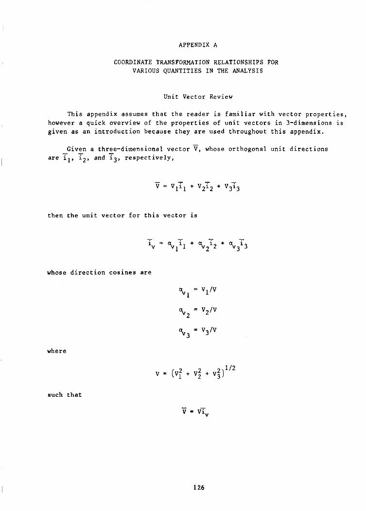
APPENDIX A

COORDINATE TRANSFORMATION RELATIONSHIPS FOR VARIOUS QUANTITIES IN THE ANALYSIS

Unit Vector Review

This appendix assumes that the reader is familiar with vector properties, however a quick overview of the properties of unit vectors in 3-dimensions is given as an introduction because they are used throughout this appendix.

Given a three-dimensional vector v, whose orthogonal unit directions - - - are il, i2, and i3, respectively,

- v = Vlil + v2T2 + v373

then the unit vector for this vector is

- - - - iv = avlil + a i + a i3

v2 v3

whose direction cosines are

a = V1/v ,1

a = V3/v v3

where

. I -

v = (v? + v2 2 + V;)l’L

such that

126

- The dot product of two unit vectors ix and? Y i s then,

- - i x ' iy = axl?,+ 4r2CL2+ ax,?,

The cross product of the same two vectors i s then

where

Note that the cross product of orthogonal unit vectors i s a uni t vector i n i t s e l f .

127

Input Chordwise Unit Vectors

In t h e input coord ina te system, (x ,y , z ) t h e input u n i t chordwise v e c t o r from f i g u r e 42 is :

where 8 is t h e l o c a l input b lade angle inc luding b u i l t - i n p i t c h .

For a swept b l ade , a poin t ( A ) along t h e b lade r e fe rence l i n e (1 /4 chord- l i n e ) i s d i sp laced i n t h e x , y p lane by an ang le 6 as seen i n f i g u r e 42, t h u s t h e input u n i t chordwise v e c t o r becomes

i n t h e c y l i n d r i c a l coord ina te system ( r , 0 , z ) where t h e input chordwise d i r e c t i o n c o s i n e s i n t h e c y l i n d r i c a l coord ina te system are:

a = c o s 0 s i n 6 ‘1,

= COS^ C O S & S I m

= s i n e aC

I Z

128

Input Thickness Unit Vector

In t h e input coord ina te system, t h e input u n i t t h i ckness v e c t o r is

- - - = - s i n 0 i + cosOiz Y

From f i g u r e 42, i n a manner similar t o t h a t of t h e input chordwise u n i t v e c t o r , t h e inpu t t h i ckness u n i t v e c t o r i n t h e c y l i n d r i c a l coord ina te system i s found t o be:

where t h e d i r e c t i o n cos ines are:

= - s i n 0 s i n 6 'Ir

= - s i n 0 cos 6 ?I#

= cos0

129

Spanwise U n i t Vector

Consider a segment of t h e b l ade r e fe rence l i n e centered about point A i n f i g u r e 43, whose end p o i n t s are denoted by t h e s u b s c r i p t s 1 and 2, hub t o t i p r e s p e c t i v e l y . The u n i t v e c t o r for t h e spanwise d i r e c t i o n a t po in t A , p o s i t i v e from hub t o t i p , can be approximated by t h e spanwise u n i t v e c t o r of t h i s segment,

where

In c y l i n d r i c a l coord ina te s t h e spanwise u n i t v e c t o r and d i r e c t i o n cos ines become r e s p e c t i v e l y

- - - - is - - as,ir + as+i4 + %,iZ

%r

as 0

= ( r2-rl )cos (/d

= ( r2+r1)sinc/d

where

1 /2 d = [r: + r: - 2r l r2cos(25) + ( z ~ - z ~ ) ~ ]

Where t h e fo l lowing approximations are made for t h e l a g ang le and r ad ius a t po in t A.

6A = (62+61)

1 rA = 7 (r1+r2)

130

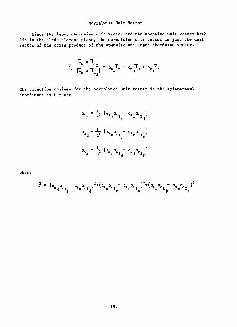
Normalwise Unit Vector

Since t h e input chordwise u n i t vec to r and the spanwise u n i t v e c t o r both l i e i n t h e b l ade element p lane , t h e normalwise u n i t v e c t o r i s j u s t t h e u n i t vec to r of t h e c r o s s product of t h e spanwise and input chordwise v e c t o r .

The d i r e c t i o n cos ines f o r t h e normalwise u n i t v e c t o r i n t h e c y l i n d r i c a l coord ina te system a r e

where

131

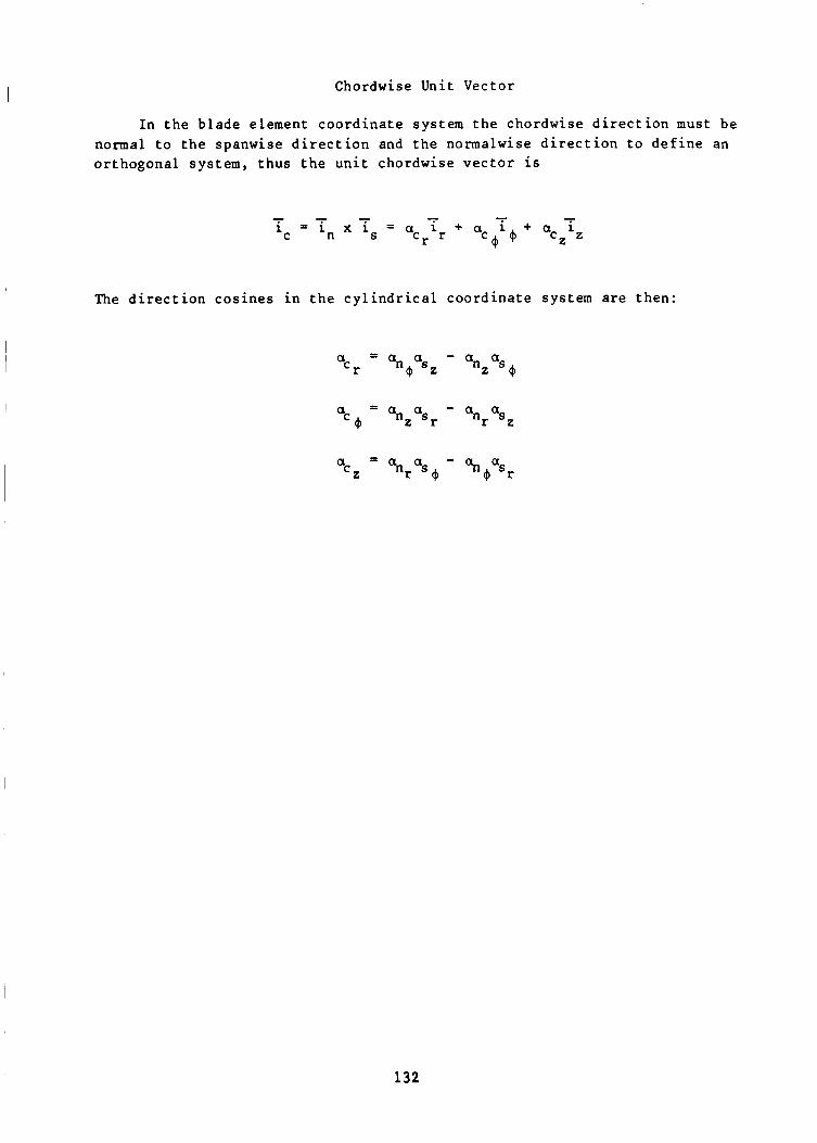
Chordwise Unit Vector

I n t h e b lade element coord ina te system t h e chordwise d i r e c t i o n must be normal t o t h e spanwise d i r e c t i o n and t h e normalwise d i r e c t i o n t o d e f i n e an or thogonal system, thus t h e u n i t chordwise v e c t o r is

The d i r e c t i o n cos ines i n t h e c y l i n d r i c a l coord ina te system are then:

132

Blade Geometry Q u a n t i t i e s i n t h e Blade Element Coordinate System

Because it i s necessary t o c a l c u l a t e t h e aerodynamic s o l u t i o n i n the b l ade element coord ina te system, t h e l o c a l input b l ade s e c t i o n p r o p e r t i e s m u s t be transformed t o t h e b l ade element system.

The b lade element chord l eng th i s obta ined from t h e inpu t b lade chord by use of t h e do t product r e l a t i o n s h i p f o r u n i t v e c t o r s .

And i n a similar manner t h e b l ade element t h i ckness is found t o be

133

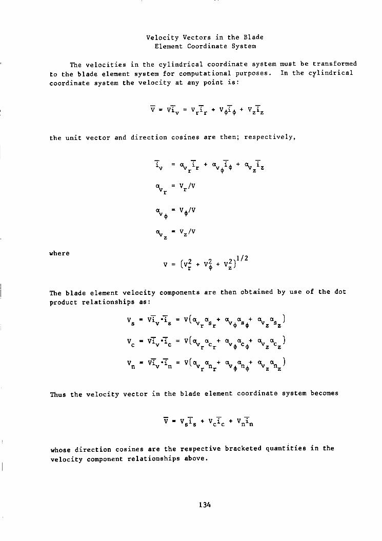
where

Velocity Vectors in the Blade Element Coordinate System

The velocities in the cylindrical coordinate system must be transformed to the blade element system for computational purposes. coordinate system the velocity at any point is:

In the cylindrical

the unit vector and direction cosines are then; respectively,

- - - - =

iV avr ir + av+io + avziz

a = Vr/V vr

The blade element velocity components are then obtained by use of the dot product relationships as:

- - V, = Vi;i = v(avrasr+ a a + av as )

V, = viv*ic = v(av + a a C + a

V, = viv*in = ~ ( a ~ a + a a + a a )

S v+ s+ 2 2

1 racr V + + vzacz

r "r v$ '4 "2 "z

- -

- -

Thus the velocity vector in the blade element coordinate system becomes

- - - - V = Vsis + Vcic + Vnin

whose direction cosines are the respective bracketed quantities in the velocity component relationships above.

134

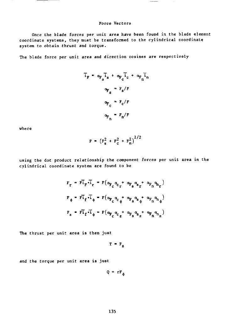
Force Vectors

Once t h e b lade f o r c e s per u n i t area have been found i n t h e b lade element coord ina te systems, t h e y must be transformed t o t h e c y l i n d r i c a l coord ina te system t o o b t a i n t h r u s t and torque .

The b lade fo rce per u n i t area and d i r e c t i o n cos ines a r e r e s p e c t i v e l y

- - - iF - - aFsis + aF ic + aFnin C

= F /F 9 s S

- F / F 'n n

where

1 /2 F = (F: + F t + F:)

us ing t h e do t product r e l a t i o n s h i p t h e component f o r c e s per u n i t area i n t h e c y l i n d r i c a l coord ina te system are found t o be

The t h r u s t pe r u n i t area i s then j u s t

T = F,

and t h e torque per u n i t area i s j u s t

Q = rFe

135

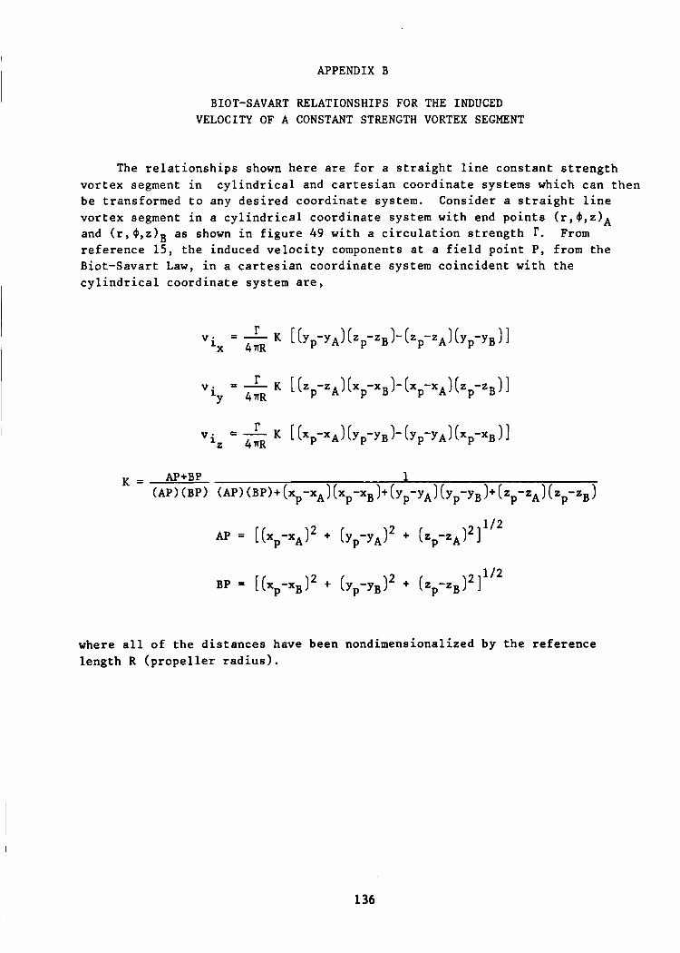
APPENDIX B

BIOT-SAVART RELATIONSHIPS FOR THE INDUCED VELOCITY OF A CONSTANT STRENGTH VORTEX SEGMENT

The relationships shown here are for a straight line constant strength vortex segment in be transformed to any desired coordinate system. Consider a straight line vortex segment in a cylindrical coordinate system with end points (r,$,zIA and (r,4,zIB as shown in figure 49 with a circulation strength r. reference 15, the induced velocity components at a field point P, from the Biot-Savart Law, in a Cartesian coordinate system coincident with the cylindrical coordinate system are,

cylindrical and Cartesian coordinate systems which can then

From

where all of the distances have been nondimensionalized by the reference length R (propeller radius).

136

Applying the standard relationships between a Cartesian and cylindrical coordinate system,

x = r cos+

y = r sin+

The induced velocity components, after some algebriac manipulation, in the cylindrical coordinate systems are,

vi = r*G*[(zp-zA)rBsin(+ P B -+ )-(zp-zB)rASin(+ P A -+ )]=r*Gcr

vi, = r*G* [ (rp-rA)sin ( +p-+A)-(rp-rB)sin( $p-+B)+r~rBsi"(+~-+B) kr*Gc,

1 AP + BP 4nR (AP)(BP)

G P -

The geometric influence coefficients (GC,, GC+, GC,) can then be transformed to the blade element coordinate system for the field point under considera- t ion.

137

Thus by the appropriate transformation the induced velocity components in the blade element coordinate system become

Vin = r GC,

Vic = r GC,

v. = r G C ~ 1s

The transformation required for this last step are shown in Appendix A.

138

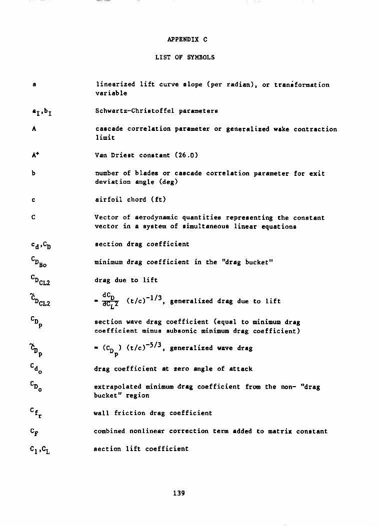
APPENDIX C

LIST OF SYMBOLS

a

a P b I

A

A+

b

C

C

'd "D

C D B ~

%L2

%A

cDP

N

P % C

cDO

f r C

CF

c1 JL

linearized lift curve slope (per radian), or transformation variable

Schwartz-Christoffel parameters

cascade correlation parameter or generalized wake contraction limit

Van Driest constant (26 .O)

number of blades or cascade correlation parameter for exit deviation angle (deg)

airfoil chord (ft)

Vector of aerodynamic quantities representing the constant vector in a system of simultaneous linear equations

section drag coefficient

minimum drag coefficient in the "drag bucket"

drag due to lift

dCD (t/c)-'l3, generalized drag due to lift = a T section wave drag coefficient (equal to minimum drag coefficient minus subsonic minimum drag coefficient)

= (C, (t/~)-'/~, generalized wave drag P

drag coefficient at zero angle of attack

extrapolated minimum drag coefficient from the non- "drag bucket" region

wall friction drag coefficient

combined nonlinear correction term added to matrix constant

section lift coefficient

139

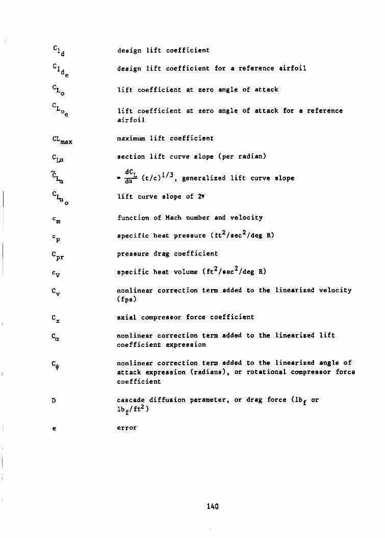
"d

de

cLO

'e cL

~ m a x

cm

?La

Ch 0

'm

P C

CPr

cV

cv

cz

cca

D

e

design lift coefficient

design lift coefficient for a reference airfoil

lift coefficient at zero angle of attack

lift coefficient at zero angle of attack for a reference airfoil

maximum lift coefficient

section lift curve slope (per radian)

* dCL (t/c)'l3, generalized lift curve slope

lift curve slope of 2n

function of Mach number and velocity

specific heat pressure (ft 2 /sec 2 /deg R)

pressure drag coefficient

specific heat volume ( ft2/sec2/deg R)

nonlinear correction term .added to the linearized velocity (fps)

axial compressor force coefficient

nonlinear correction term added to the linearized lift coefficient expression

nonlinear correction term added to the linearized angle of attack expression (radians), or rotational compressor force coefficient

cascade diffusion parameter, or drag force (lbf or lbf/ft2)

error

140

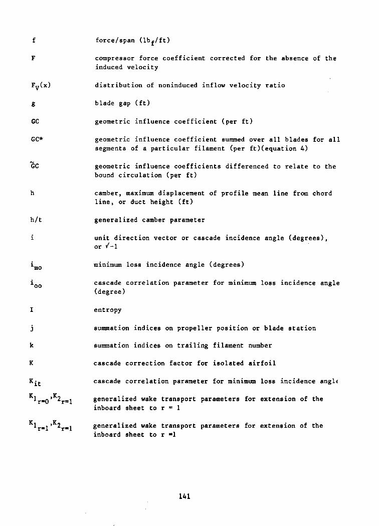
f

F

h

h/t

i

imo

I

k

K

Kit

force/span (lbf/ft)

compressor force coefficient corrected for the absence of the induced velocity

distribution of noninduced inflow velocity ratio

blade gap (ft)

geometric influence coefficient (per ft)

geometric influence coefficient summed over all blades for all segments of a particular filament (per ft)(equation 4)

geometric influence coefficients differenced to relate to the bound circulation (per ft)

camber, maximum displacement of profile mean line from chord line, or duct height (ft)

generalized camber parameter

unit direction vector or cascade incidence angle (degrees), or 4-1

minimum loss incidence angle (degrees)

cascade correlation parameter for minimum loss incidence angle (degree)

entropy

summation indices on propeller position or blade station

summation indices on trailing filament number

cascade correction factor for isolated airfoil

cascade correlation parameter for minimum loss incidence angle

generalized wake transport parameters for extension of the inboard sheet to r = 1

generalized wake transport parameters for extension of the inboard sheet to r =I

141

cascade correlation parameters for deviation angle

1 summation indices on segment number of a trailing filament

L lift per unit span (lbf/ft), or duct wall length, .or number of propeller positions

sumation indices on blade number m

M Mach number or matrix of aerodynamic and geometric influence coefficients for a system of simultaneous linear equations

critical Mach number

cascade correlation parameter for deviation angle M,

n cascade correlation parameter for minimum loss incident angle, or normal coordinate (dimensionless)

n cDO empirical cascade correlation parameter

nD DBO empirical cascade correlation parameter

Reynolds number, rrQ ,Ur/wr(dimensionless) NR

P static pressure (lbf/ft2 1, or power (ft lbf/sec)

Base Pressure ( lbf/ft )

2 total pressure (lbf/ft 1

2 PB

PO

turbulent Prandtl number (dimensionless) PrT

heat flux

radial coordinate in the cylindrical coordinate system r

blade tip radius (ft) R

gas constant ( ft2 /sec2 /deg R) R

radial coordinates of selected generalized wake features nondimensionalized by the blade radius

142

TO

t IC

U

'e

uz

u4J

U+

V

v

imom

V t

W

X

Y

Y+

z

2

'Bm

streamwise coordinate (dimensionless)

maximum airfoil thickness (ft)

compressor force (lbf), or temperature (deg R), or. thrust (Ibf)

total temperature (deg R)

generalized thickness parameter

magnitude of velocity, or velocity component ( fps)

total cascade velocity including induced velocities (fps)

axial cascade velocity component ( fps)

rotational cascade velocity component ( fps)

universal velocity (dimensionless)

induced velocity ( fps)

velocity as defined where used in text (fps)

momentum induced velocity ( fps)

wake transport velocity ( fps)

complex coordinates in duct plane (r + iz)

coordinate along the pitch axis in the Cartesian coordinate system

chordwise coordinate in the Cartesian coordinate system

universal distance

axial coordinate in the cylindrical and Cartesian coordinate system

axial distance, z/rr (dimensionless)

cascade minimum loss

143

W compressor momentum induced v e l o c i t y ( f p s )

a

‘e

a i

‘min

a max

O O

S u b s c r i p t s

B

C

f r

H

i

i , L p

n

Pr

r

angle of a t t a c k or cascade flow angle or swirl angle t o a x i s (deg)

angle between Ue and a x i a l d i r e c t i o n (deg)

cascade inc idence angle (deg)

angle of a t t a c k f o r %Bo (deg)

angle of a t t a c k fo r CLmax (deg)

cascade s t agge r angle (deg)

angle of a t t a c k fo r zero l i f t (deg)

due t o bound v o r t e x

blade element chordwise d i r e c t i o n

due t o s k i n f r i c t i o n fo rce

hub c o n d i t i o n s

of a p r a t i c u l a r inflow s t a t i o n

summat ion i n d i c e s

blade element normalwise d i r e c t i o n , o r i n the d i r e c t i o n of t h e norma 1

due t o p re s su re f o r c e

r e fe rence cond i t ions , based on s t r u c t u r a l sea l e v e l atmos- phe r i c cond i t ions fo r a l l thermodynamic q u a n t i t i e s . The r e f e r e n c e rr is the i n l e t ou te r r a d i u s , and the v e l o c i t y is the mean i n l e t v e l o c i t y .

b lade element spanwise d i r e c t i o n , or i n t he streamwise d i r e c - t ion

t i p cond i t ion

144

Tip

TR

Superscripts

V

a 2c

= 20 a*

B

Y

r

6*

& O

00

A

A *

E

5

blade tip

due to trailing wake

wall conditions

freestream value, or stagnation conditions

inlet of the blade row

exit of the blade row

freestream or edge of boundary layer

iteration number

mean or average quantity or indicates vector

corrected exit flow angle due to back pressure (deg)

angle of attack for ‘Do (deg)

metal angle of blade camberline at trailing edge relative to the stagger angle (deg)

flow swirl angle (deg)

ratio of specific heats or boundary layer thickness (ft)

circulation of vortex segment (ft2/sec>

boundary layer displacement thickness ( ft)

flow deviation angle from the metal angle

cascade correlation parameters for deviation angle (deg)

boundary layer thickness, 6 /rr (dimensionless)

boundary layer displacement thickness, 6*/rr (dimensionless)

empirical correction factor for lift curve slope

= (M2-1) (t/~)-~’~, generalized Mach number

145

0*

OB

K

x

P

' nss' n+

I+

Q B

X

n

transformed normal coordinate (dimensionless)

geometric blade pitch angle or blade pitch angle of streamline to axis (deg)

boundary layer momentum thickness ( ft 1

local geometric blade pitch angle in the blade element coordinate system (rad)

von Karman constant (0 .41)

generalized wake contraction parameter for the tip vortex or thermal conductivity (lb/sec/deg R)

viscosity ( slugs/ f t /sec)

pressure ratio, p/pr

density (slugs/ft3)

stress components

stress T /T (dimensionless 1

reference coordinate in the cylindrical coordinate system (rad), or inflow angle (rad)

blade dissipation function, rate of dissipation of energy of the propeller boundary layer

effective camber angle (deg)

empirical curve fit relationship

Clauser constant (0.016) (dimensionless) or transformation func t ion

stream function (slugs/ft)

wake age or wake azimuth position (deg or rad) - see section entit led "Generalized Wake Model"

propeller rotational speed (rad/sec)

146

A$O

DBO

AC

A i

AaO

A aO

a2 A

twice $0

twice C DBO

twice the minimum l o s s incidence angle (deg)

cascade correction for zero angle of attack

(deg) angle of attack for

*' (deg) angle of attack for

DBO

DBO

147

P w

> w 2 . 0

I

z

I

Y

a

h m 1 U m C 0 .rl U m

. . . . . . . . I . . . . . . . .

r - w k ~ & m 6 Q . . . . . . . . I . . . . . . . .

P

z 5

I

v) U 4 Z S Z Z : % % % ; a

00000000 I ? ? ? a ? ? ? ? ?

m m m m u u g u o m m m m m m m 00000000 m w m m m m m m . . . . . . . .

tlJ V C

E 0

N N N N 0 0 0 0 * * * * m m m m N N N r J d d d d m m w w w w w w . . . . . . . . 1 I . . . . . . . .

. . . . . . . .

d Y z nl Ln

z W

aJ 9 m

148

I .1.-. . . . . . . . . . . . . . . . . . . . . h a 3 U v3

C 0 .r( U m .I4 Lc

d 0

.I4

3 0)

m 3 a

2

' .5

& b

a J - 0 u a e o m s

O Q , w 3 Lco QlPl Pl

F 0) *I4

r l v ) r l a J 0 , E l a O N Lco P 4 0

rl a a l a urn 0 . .I4 0 a aJ II

k X U U

01 rl P m w

. . . . . . . . - . . . . . . . . . . . . . . . .

I . . . . . . . . I . . . . . . . .

I . . . . . . . .

I .-. . . . . . . I . . . . . . . .

149

. . . . . . . . Ll 0) C C .r( a rn

I . . . . . . . .

. . . . . . . . I . . . . . . . . 0 - ua3 L l . 5 0 PI

Ii .isl. 0 1

1 - . . . . . . . . I . . . . . . . .

H H H

Q) d D ra H

I

150

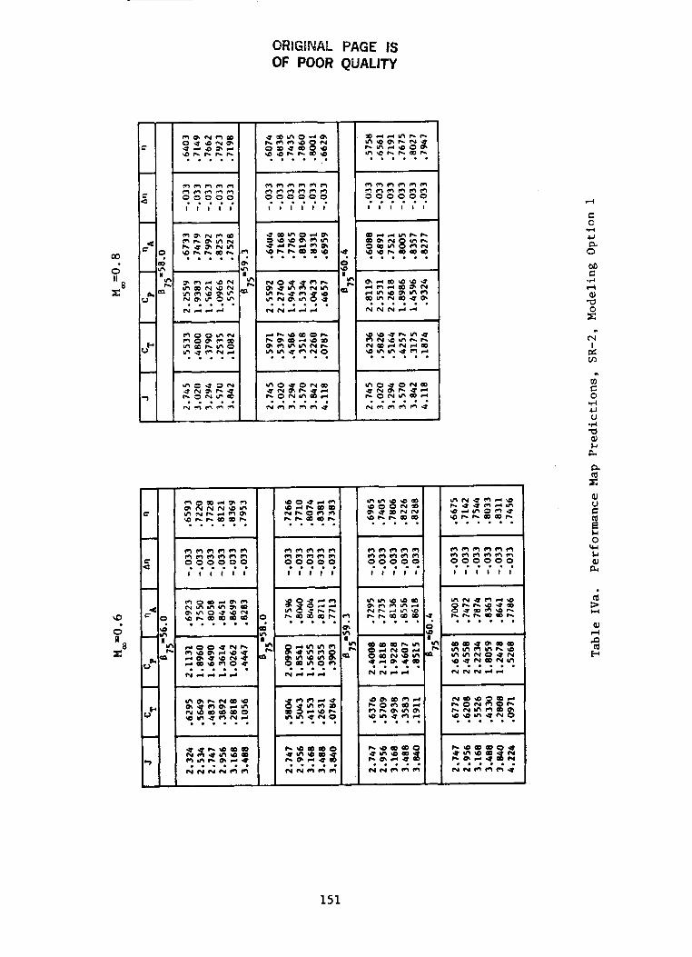
ORIGINAL PAGE fS OF POOR QUALITY

co 0 II

c 8

9

0 II

c 8

. . . . . . “ d d d

-lu+

I m o m m m m m n m m m m ? ? ? ? ? ? I I I I I I I ;I 9 In h

I I

rl

C 0

.I4 U a 0 M C

.rl d b)

m

r( u V rl a a, Ll

p1

(d z a, rl

w 8

151

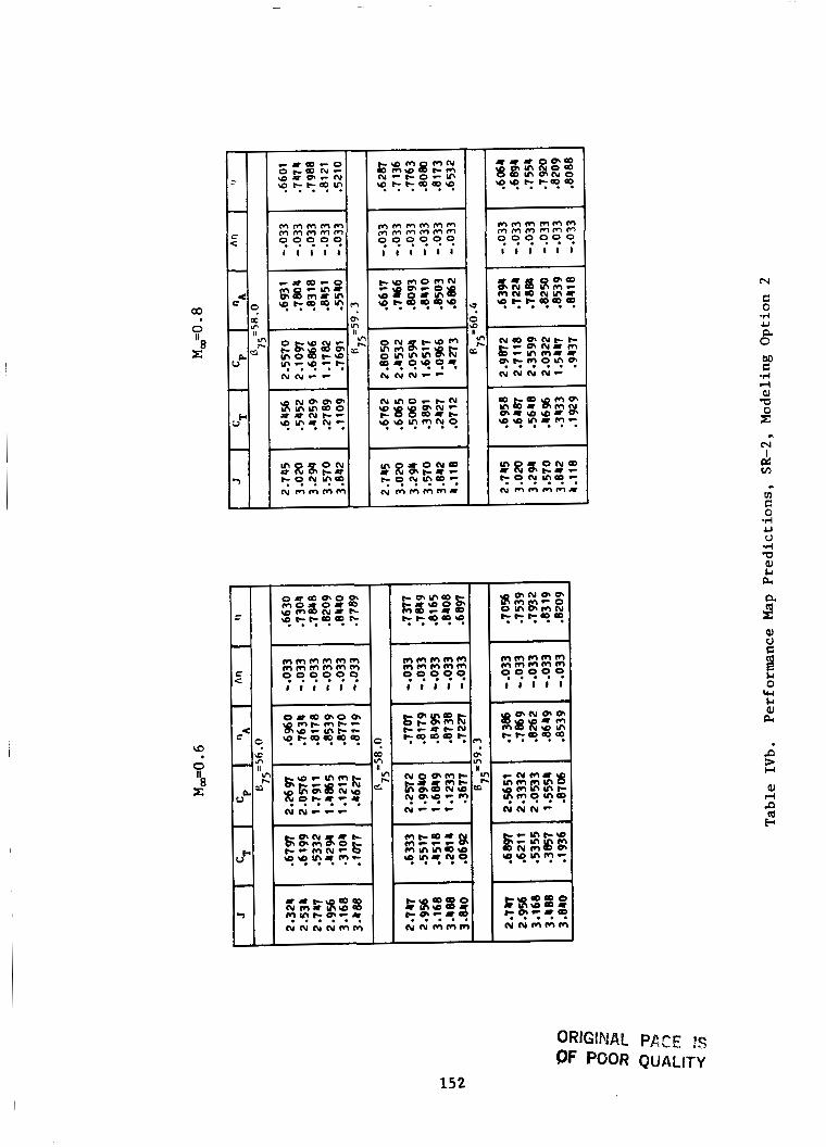
03

0

8 II

r:

m m m m m m m m m m

I 1 1 1 1 9 9 9 9 9

a 0 II 8 c

m m m m m m m m m m m m m m m m m m m m m m m m m m m m m m m m

1 1 1 1 1 1 I l l 1 1 1 8 1 1 1

- r I .

ORIGINAL PACE IS (IF POOR QUALITY

II) C 0 .rl U U .d

P z aJ rl P ([I CI

152

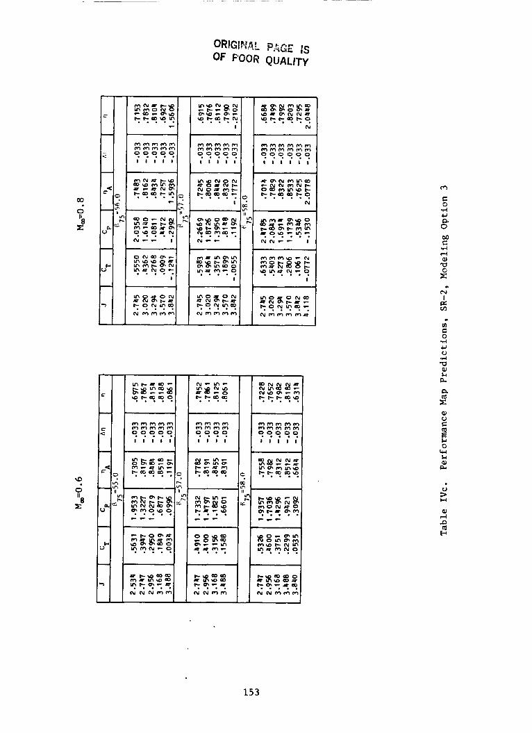
ORlGiFEAE PAGE IS OF F'OOW QUALITY

00

0 II 8 t:

\o

0 8

II

t:

m m m m m m m m m m m m m m m m m m m m m m m m m m m m m m m m

I 1 l 1 1 S

-+-

m m m m m m m m

I I I I

m m m m m m m m m m

+-- +I VI h

a = u I I - - - I I - - -

m m m m m m m m m m I 3 9 9 9 9 1 1 1 l 1 L

I_Cr

C 0 r( U a 0

.

m C 0

aJ U C

& 0 2

153

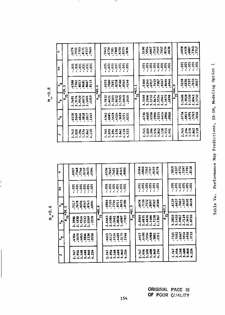
co 0 II

E 8

\o

0 II

c 8

c a

-

---

I r r d d d d d 0 n n n 0 0

I I I I I I 9 9 9 9 9 9

I

154

ORIGINAL PAGE SS OF POOR SLrfiLITY

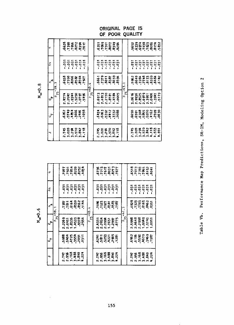
ORIGINAL OF POOR

PAGE IS QUALITY

I

~ . . . . . . . . qlff::f? 9 9 9 9 9 9 -I- .---- m m m m m m ? ? ? ? ? ?

1 1 1 1 1 1

03

0 8

II

r: U a 0 M c .rl .-I 'ai a r"

H+

0 Iy

I 1 1

\o

0 8

II

E 0 3

I I I ( u ~ m m m u

155

03

0

8 I1

z

\o

0

2

I C C l - C C

m m m m m 9 9 9 9 9

I 1 1 1 1 J

I

rl

C 0 .d u a 0

M C

I d L n

a r" aJ V C (d E Li 0 w Ll a a

V 3 a rl P (d w

156

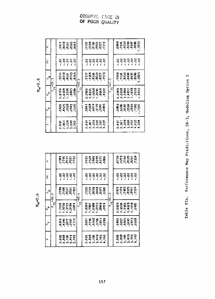
co 0

8 II

c

L D

0

8 II

c

I

N N N N N N N N N N N N

1 1 1 1 1 1 1 1 1 l 1 1

N

C 0

.I4 u

0" W

e m

e

rd W 3

15 7

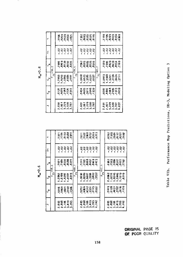
a3

0

8 II

z

\D

0 8

I'

E

I I - - - -1'

C l c - ? ? ?

N N N N N

I I I I I 3 9 9 9 9

I I I - - - -

~ m m m m m o m m - W O C D N V I

y ? ? ? ?

N N N N N

I 1 1 1 1 9 9 3 3 3

I " m m m

CUNNNNN 9 9 9 9 9 9 I l l l l I

N N N N N N

I I I I I I 9 9 9 9 9 9

m C 0 4 u a 0 M C

I $ v) C 0

Ll 0 w

n U i aJ

158

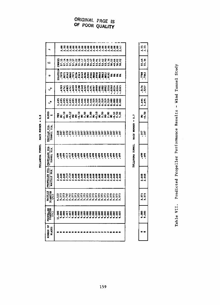
a w u u i

ORIGINAL PAGE BS OF POOR QUALITY

......................

m a a m m m a a a a a a a a a a a a a a a a 0 0 0 ~ ~ 0 0 0 0 0 0 0 0 0 0 0 0 0 0 0 0 0

N N N N N N N N N N N N N N N N N N N N N N 444~"q444444q44qqq44qq

~ n n m m n n n n n n n n n n n n n n n ~ o N C h Q U h C C C h h h h C h C h C C C h L dnnchnnnnnnnnnnnnnnnnn ......................

h -0 1 U CA

C C 1 t+

01 a 0 Ll PI

U al U L)

159

m o o 0 0 a n

. . . . .

160

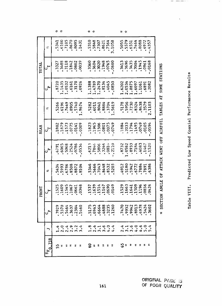
. . . . . . . . . . . . . r l r r r r I r ( N r ( d d I

. . . . . . . . . . . . . rr rr N I * - - * * -

. . . . . . . . . . . . . 1 I I I - = * * - *

. . . . . . . . . . . . . I 1 rr I I * - * * - *

m U l-l 1 m 8 al U e Q E

x Q 0 u

H H H 3 al rl D 8

161

( A ) EFFECT O F HAC11 NUMBER

SPINNER A, 0 BLADES

.3353

.3012

.2595

.2147

.1642

.%Ob

.3002

.2460

.1726

.21 io

,4034 .6509 .6904 3.261 .7307 .6799 .3503 .7127 .7640 2.020 .6515 ,7394 .2049 .7572 .a160 2.354 -5444 .7069 .2123 .7076 .0433 1.007 .4270 .0144 .1209 .7969 .a021 1.395 -2931 .7992

,4581 .6203 .6060 4.466 .0107 .6598 .3676 .6934 -7769 3.671 .6750 .7364 .2625 .7356 .0326 2.061 .5093 .7026

.1330 .7344 ,7607 1.959 .3056 .7489

.2004 .7449 . m i 2.413 .4ii4 .?a45

6 5 64.2 3.2 1.500 1.766 .2934 .3303 .6225 6 5 64.2 3.6 1 . 5 7 3 1.849 .2929 .3513 .6705 6 5 64.2 4.0 1.573 1.030 .2000 .3372 .7117 65 64.2 4.4 1.303 1.607 .2370 .2003 .7541 6 5 6 4 . 2 4.0 1.077 1.190 .1673 .I900 .7456

.5904 3.275 .6237 .6095

.6040 3.422 ,6442 .6770

.7337 3.411 .6172 .7236 ,7092 2.990 .5253 .7730 .7933 2.275 .3653 ,7707

,2952 .2954 .2033 .2417 .1734

.3260 .6253 .5920

.3474 .6751 .6746

.3319 .7109 .7216

.2707 .7665 .7735

.1030 .7675 .7636

MACH 0.6

60 60 60 60 60

65 65 65 6 5 65

50 50 50 50 5R

62.5 62.5 62.5 62.5 62.5

3.0 3.2 3.4 3.6 3.0

3.5 4.0 4 . 3 4 . 6 4.8

- .6051 .6606 .?103 .7394 .6790

.5799 ,6743 .7260 ,7137 .6300 -

ElACH 0 . 7

1.529 . 2 a w .jig6 .sa25 .6270

.7549 ,1055 .1506 .7256 .7563

1.322 .2642 .2067 .6431 .6939 1.051 .2202 .2304 .6920 .7455

.4490 .1367 .0722 .7229 .6100

2.300 .3200 .4010 .5524 .bo46 1.060 .2900 .3319 .6344 .7135 1.209 .2308 .2263 .6070 .7724 .9077 .1940 .1509 .6936 .7399 .6680 .1510 ,0017 .6699 .5864

- .bo85 .5509 ,4506 .3441 .2069

.7290

.6219

.4571

.3529

.2327 -

58 58 58 50 58

3.0 3.2 3.4 3.6 3.0

3.6 4.0 4.4 4.6 4 .0

3.017 2.637 2.171 1.675 1.150

4.530 3.600 2.767 2.274 1.751 -

1.325 1.120

2.143 1 * 020 1.470 1.206 1.002

60

6 5

- 60 60 60 60 60

65 65 65 65 65 -

62.5 62.5 62.5 62.5 62.5

ElACll 0 . 8

.4352 ,2707 ,1614

.5200 ,5072 .4196 .3296 .2130

.6100

.6050

.5257

.4721

.5610

.6070

.6026

.5201

2.203 1.521 1.105

NEGATIVE THRUST-NO S O L ~ T T I O N I I I NEGATIVE TtiPJJST-10 SOJ.UTION I

3 . 0 4.0

3.009 3.431 2.034 2.351 1.022

.2403 .2005 . 4433 .5009

.2426 .2646 .5236 .6021

.2125 .2071 .5721 .6476

.1015 .1401 .5065 .6236

.1422 .0716 .5726 .4575

( B ) EFFECT OF S P I N N E R SHAPE

6 BLADES, MACH 0.7

L 3.277 3.429 3.415 2.972 2.240

.6220

.6420

.6152

.5204

.3572

1.767 1.054 1.039 1.505

1.511 1 . 5 7 5 1.576 1.307

* OFF A I R F O I L TABLES I N ANGLE O F ATTACK RANGE

T a b l e IX. P r e d i c t e d Moderate Speed

162

Coaxial

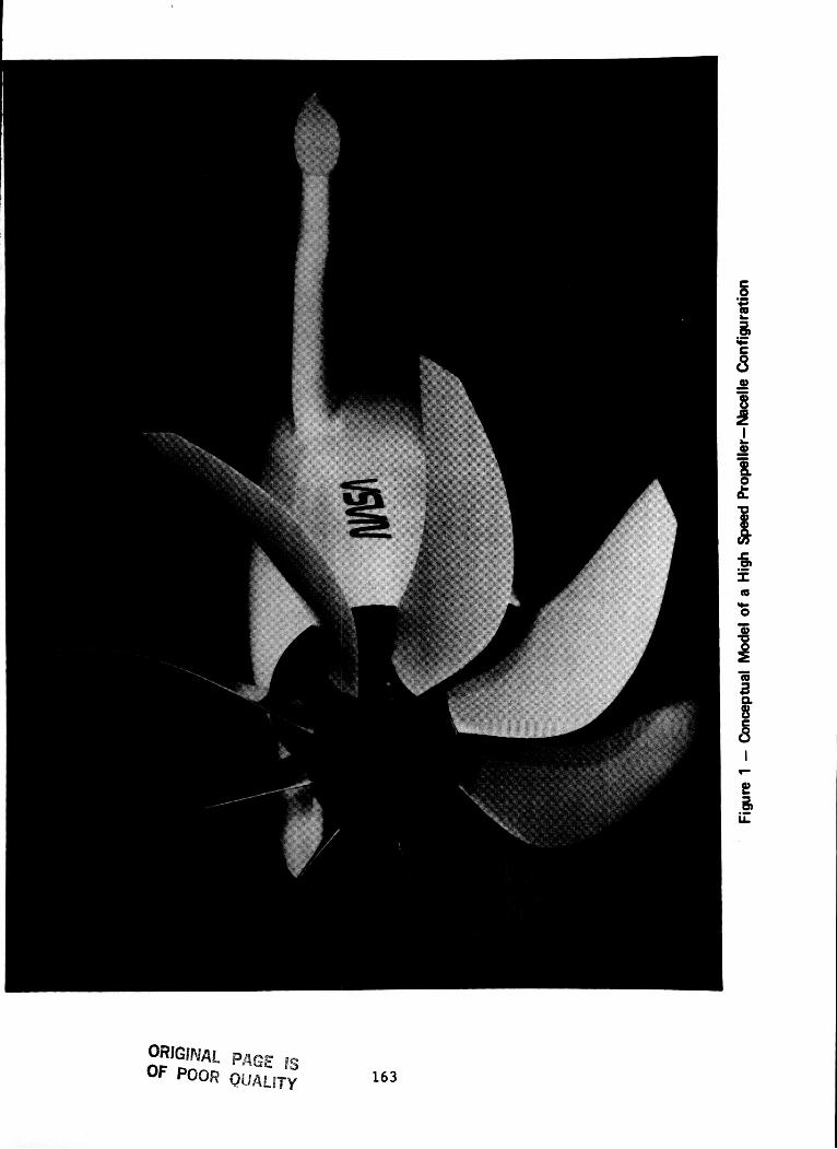
163

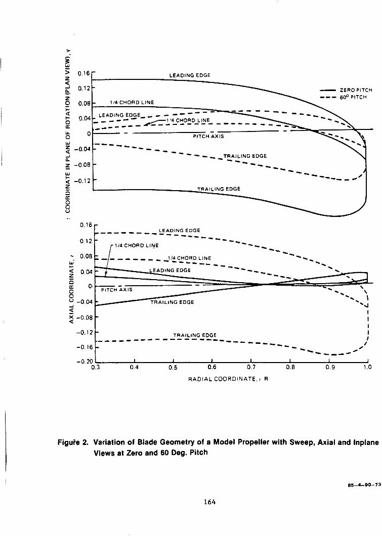
0.16-

0.12

0.08

c).04

0 w 5 -0.04 A 0 Z, -0.08 Ly + z a -0.12

h -

0.16 r

LEADING EDGE

- ZEROPITCH --- 60'PlTCH

- - 114 CHORD LINE

LEADING EDGE- - e - -- - - - _----- -1 '4 CHOR - - - - - - -

' - - - - - - - ---- - - - - - -TRAILING EDGE

- - -- - -- --- -- I -* ---- - d 0 -

TRAILING EDGE

0.12

0.08

0.04

01

-0.04

t - 2 -0.08 I U

-0.20 I I I t I 1 I I 0.4 0.5 0.6 0.7 0.8 0.9 1 .o 0.3

RADIAL COORDiVATE. 1 R

Figuie 2. Variation of Blade Geometry of a Model Propeller with Sweep, Axial and lnplane Views at Zero and 60 Deg. Pitch

85-4-90-73

164

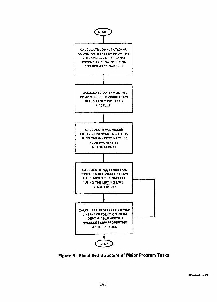
CALCULATE COMPUTATIONAL COORDINATE SYSTEM FROM THE

STREAMLINES OF A PLANAR POTENTIAL FLOW SOLUTION

FOR ISOLATED NACELLE

CALCULATE A-XJSY MMETR IC COMPRESSIBLE VISCOUS FLOW

FIELD ABOUTTHE NACELLE USING THE EFIING LINE

BLADE FORCES

CALCULATE AXISYMMETRIC COMPRESSIBLE INVISCID- FLOW

FIELD ABOUT ISOLATED NACELLE

e

CALCULATE PROPELLER LIFTING LINEWAKE SOLUTION USING THE INVISCID NACELLE

FLOW PROPERTIES AT THE BLADES

CALCULATE PROPELLER LIFTING L INEWAKE SOLUTION USING .

Figure 3. Simplified Structure of Major Program Tasks

85-4-90-72

165

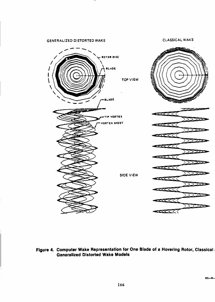
GENERA L l ZED DISTORTED WAKE

TOP VIEW

- / ---

CLASSICAL WAKE

IP V O R T E X

T E X W E E 1

SIDE VIEW

Figure 4. Computer Wake Representation for One Blade of a Hovering Rotor, Classical i Generalized Distorted Wake Models

05-4-

166

2 -

n A -T J

NACELLE BODY OUTLINE

\ \ x, PITCH AXIS

Figure 5. Cylindrical and Cartesian Coordinate Systems for Propeller Geometry

167

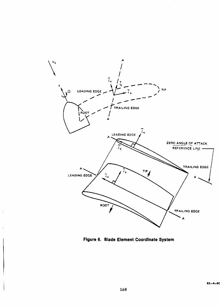
A

I I

0 / TRAILING EDGE n

Figure 6. Blade Element Coordinate System

168

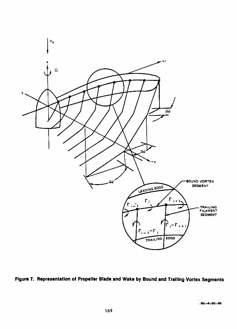
I "O

Figure 7. Representation of Propeller Blade and Wake by Bound and Trailing Vortex Segments

I '85-4-00-60

169

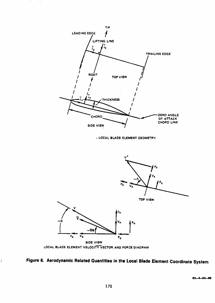
THICKNESS

ZERO ANGLE / OF AlTACK

CHORD LINE

CHORD

SIDE VIEW

- LOCAL BLADE ELEMENT GEOMETRY

TOP VIEW

f n

SIDE VIEW LOCAL BLADE ELEMENT VELOCITVECTOR AND FORCE DIAGRAM

Figure 8. Aerodynamic Related Quantities in the Local Blade Element Coordinate System

170

:D

Figure 9. Vector Diagram of Drag Forces in the Blade Element Coordinate System

86-4-9047

171

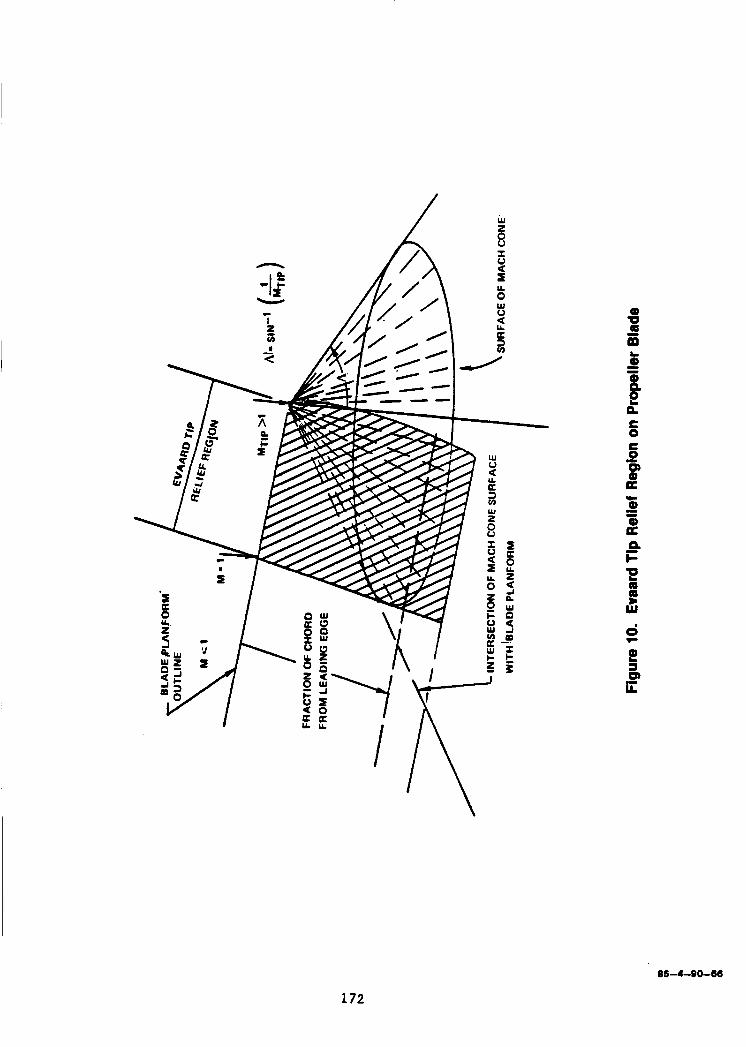
85-4-90-66

172

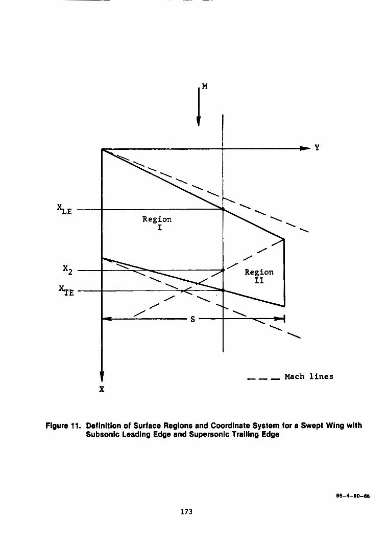
1"

x2 -

%E -

I W Y

Region I

- - - Mach l i n e s X

Figure 11. Definition of Surface Regions and Coordinate System for a Swept Wing with Subsonic Leading Edge and Supersonic Trailing Edge

86-4-9046

173

L I a

86-440-64

174

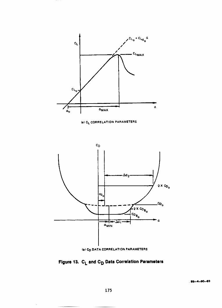
I 4

a - QMAX

(11 CL CORRELATION PARAMETERS

(bl CD DATA CORRELATION PARAMETERS

Figure 13. CL and CD Data Correlation Parameters

175

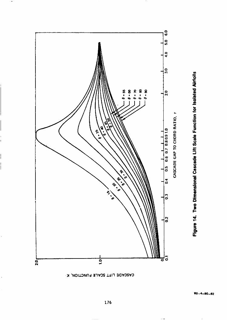
1 c

>I 'N0113Nnj 31V3S Id11 3OV3SV3

176

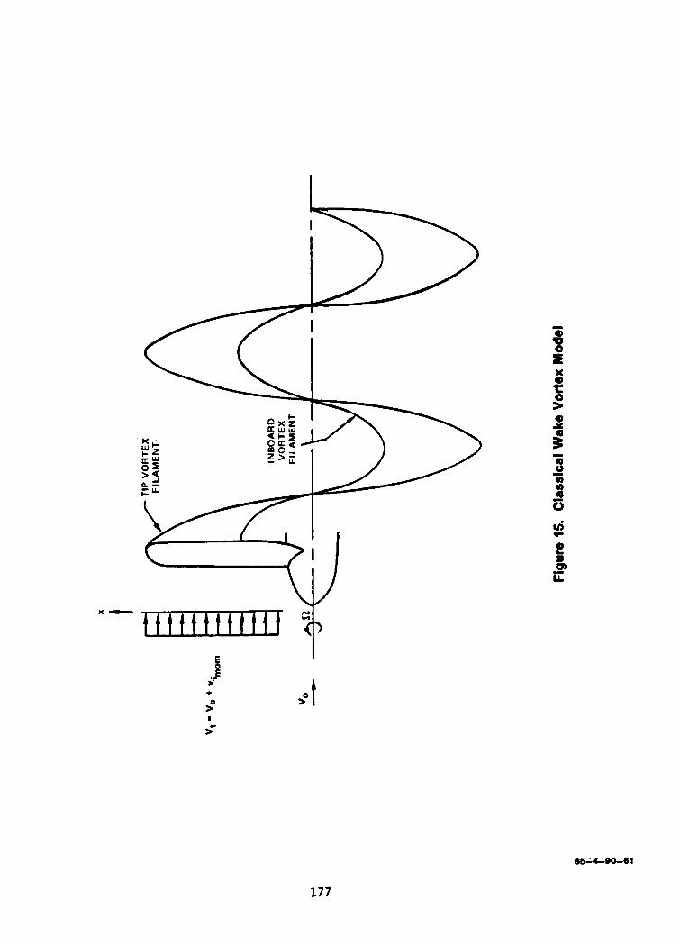
x-

t t t t t t t t t t t

+ >" >- I

>" t

177

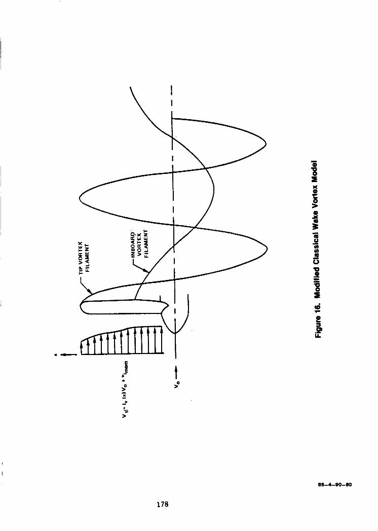
178

-- RADIAL LOCATION OF MAXIMUM CI RCU LAT ION

VORTEX SHEET CROSS SECTION

Figure 17. Characteristics of the Generalized Wake Model

88-4-00-80

179

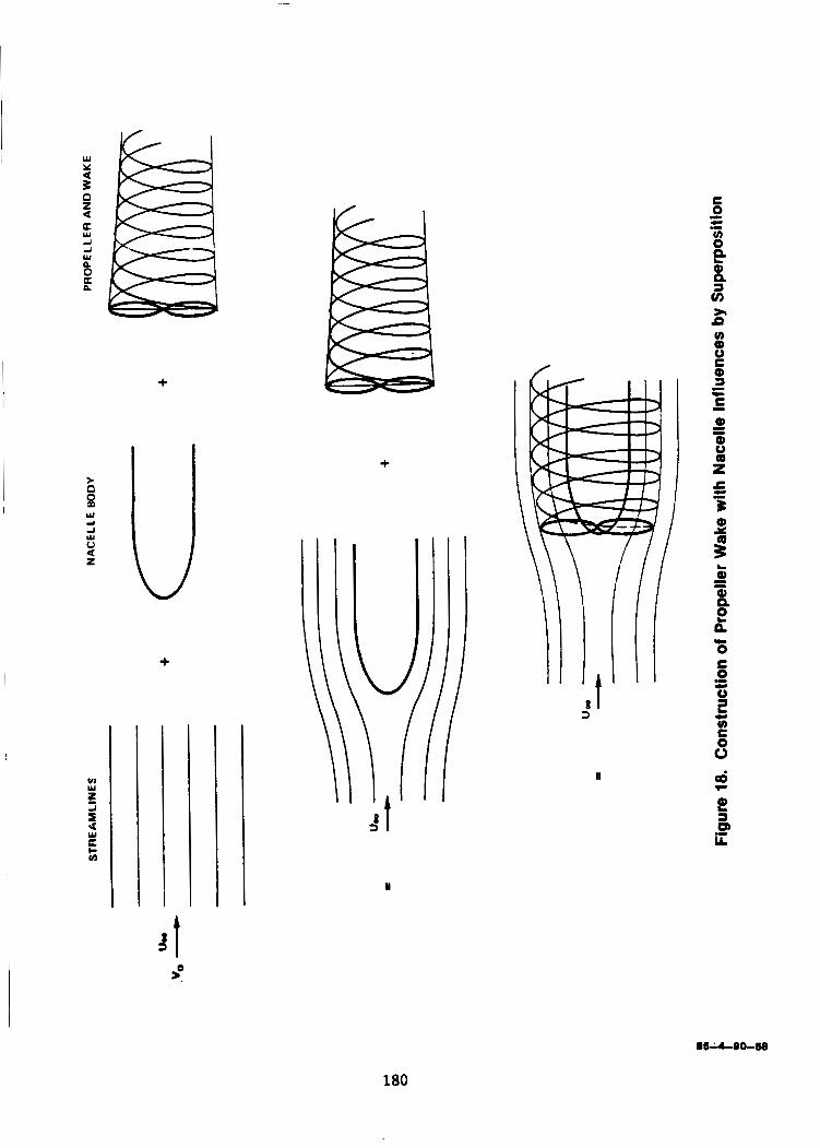
w Y

2 0 z a

+

> 0 8 w 4

Ly V

z a

+

W8 w L I u f v)

I

+

180

\"O

rmx Flgun 18. Modollng the Wako Rollup wlth Dl8cnto VOrtlC.8

181

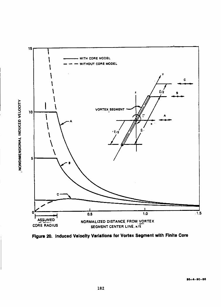
15 I I I - WITH CORE MODEL - - - WITHOUT CORE MODEL

'1 0

5

I I I I

I \ VORTEX SEGMENT -

0 / I I

0.5 1 .o . 1

NORMALIZED DISTANCE FROM VORTEX SEGMENT CENTER LINE, x - / r

ASSUMED ' CORE RADIUS - ---

Figure 20. Induced Velocity Variations for Vortex Segment with Finite Core

1

5

182

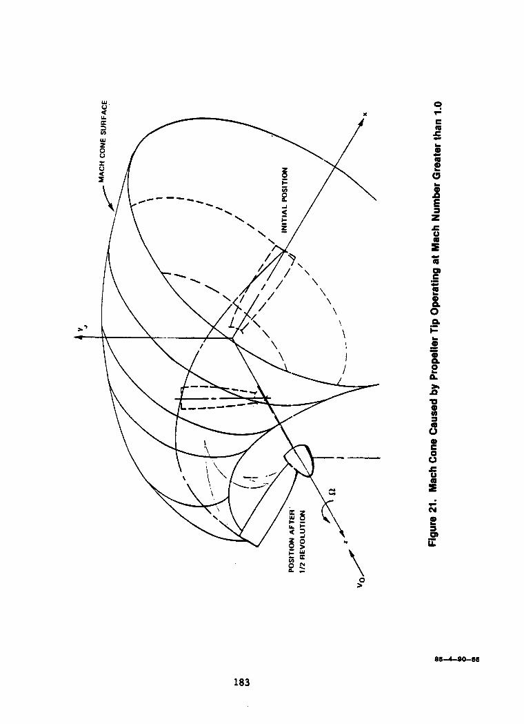
P i=

86-440-66

183

DIRECTION OF FLIGHT

TIME I14 REV. - A

I I Z R E V . = B

314 REV. - C

I REV.- D

TIME - 0

INITIAL POSITION

Figure 22. Propeller Vortex Lines and Relative Positions

86-440-64

184

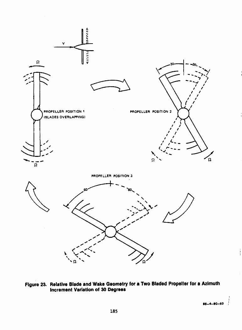
n

a PROPELLER

PROPELLER POSITION 3

\ *\ '

\ \ * a - Figure 23. Relative Blade and Wake Geometry for a Two Bladed Propeller for a Azimuth

Increment Variation of 30 Degrees

85-4-80-53 1 185

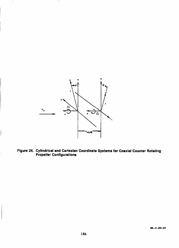
. X x

Figure 24. Cylindrical and Cartesian Coordinate Systems for Coaxial Counter Rotating Propeller Configurations

85-4-0042

186

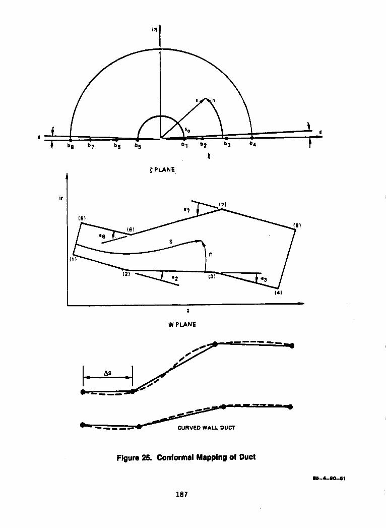
ir

W PLANE

CURVED WALL DUCT

Figure 25. Conformal Mapping of Duct

86-4-0041

18 7

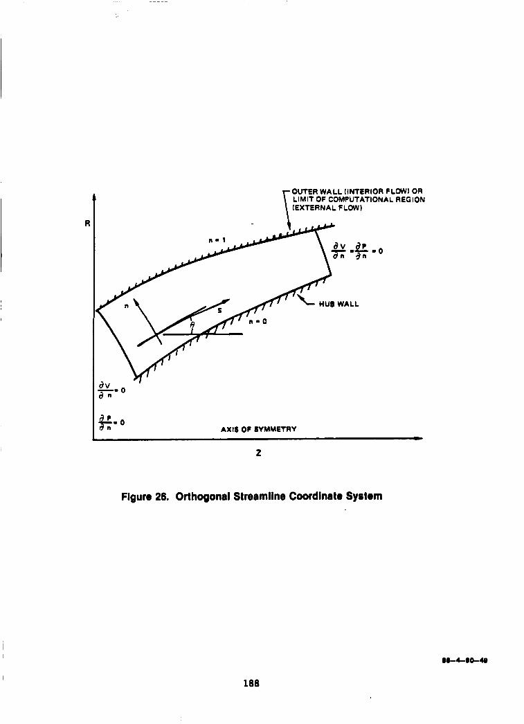
R

OUTER WALL fINTERIOR FLOW) OR LIMIT OF COMPUTATIONAL REGION (EXTERNAL FLOW)

- 0

AXIS OF SYMMETRY

z 4

Figure 26. Orthogonal Streamline Coordinate System

188

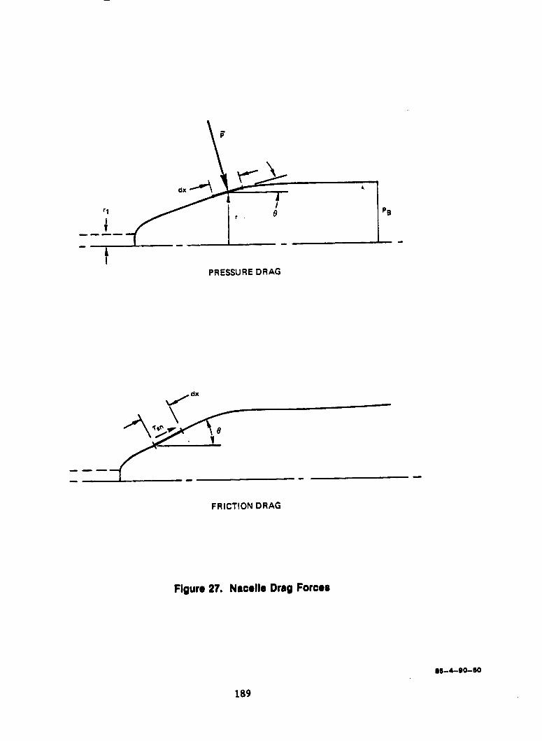
A I

PRESSURE DRAG

FRICTION DRAG

Figure 27. Nacelle Drag Forces

189

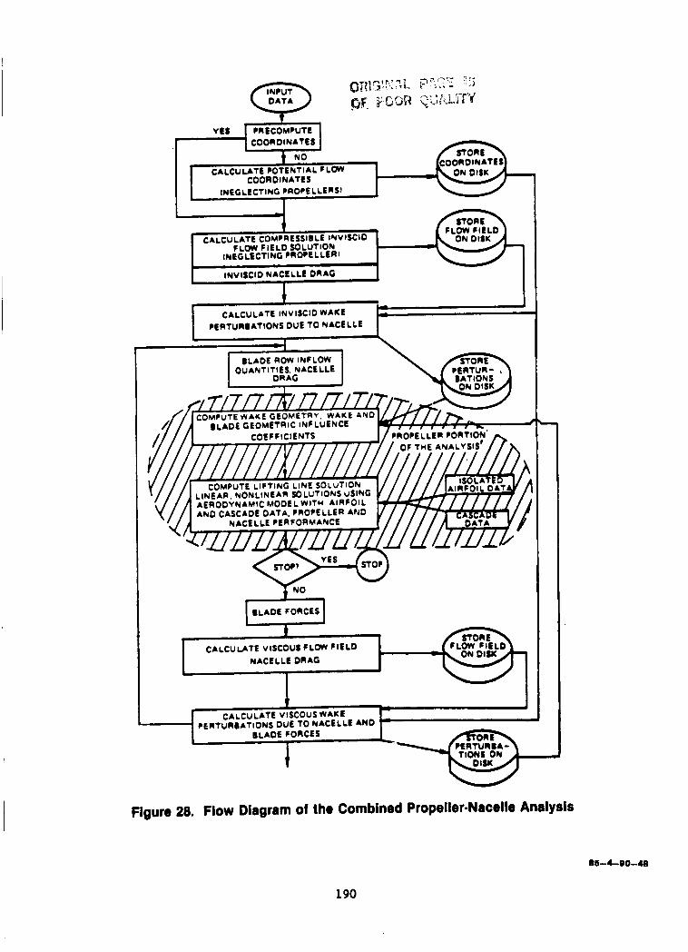
COORDINATES

COORDINATE 5 INEGLECTING PROPELLERS)

I -

ESSIOLE INVISCID 1

I 1 I

INVISCID NACELLE DRAG

t r

CALCULATE INVISCID WAKE r

PERTURBATIONS DUE TO NACELLE

NACELLE DRAG

Figure 28. Flow Diagram of the Combined Propeller-Nacelle Analysis

86-4-00-48

190

84-6-73-1

191

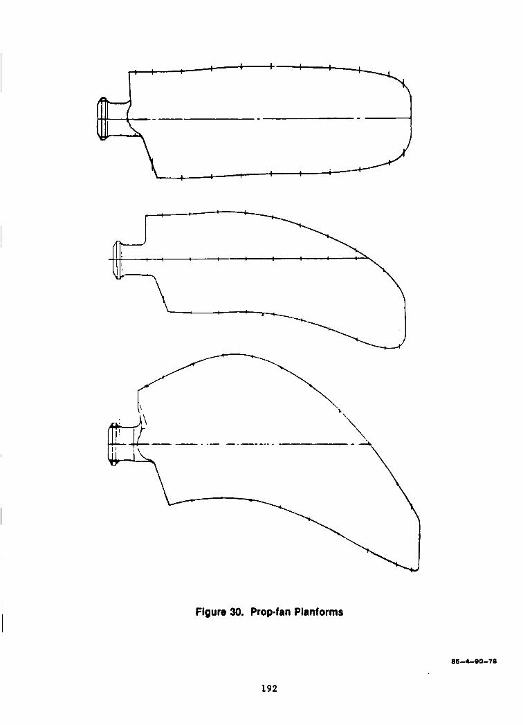
Figure 30. Prop-fan Planforms

85-4-90-70

192

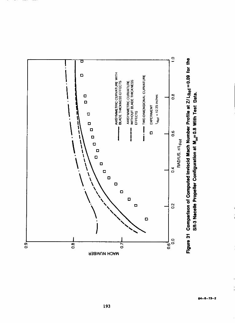
84-6-73-2

193

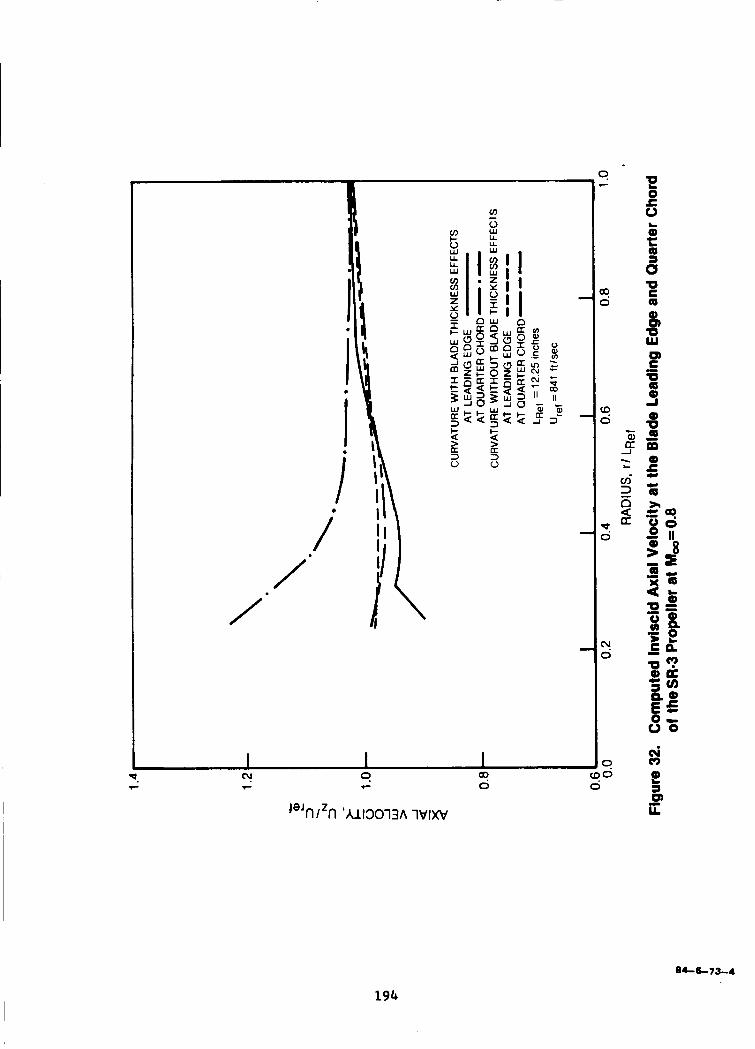
e

/ /-

/-

194

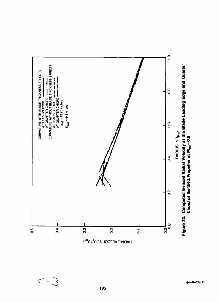
x 00 0

7. 2 2 0

=--3

0

2

s 0

0

0

P

3 (R

Q, P

Y Q,

04-8-73-3

195

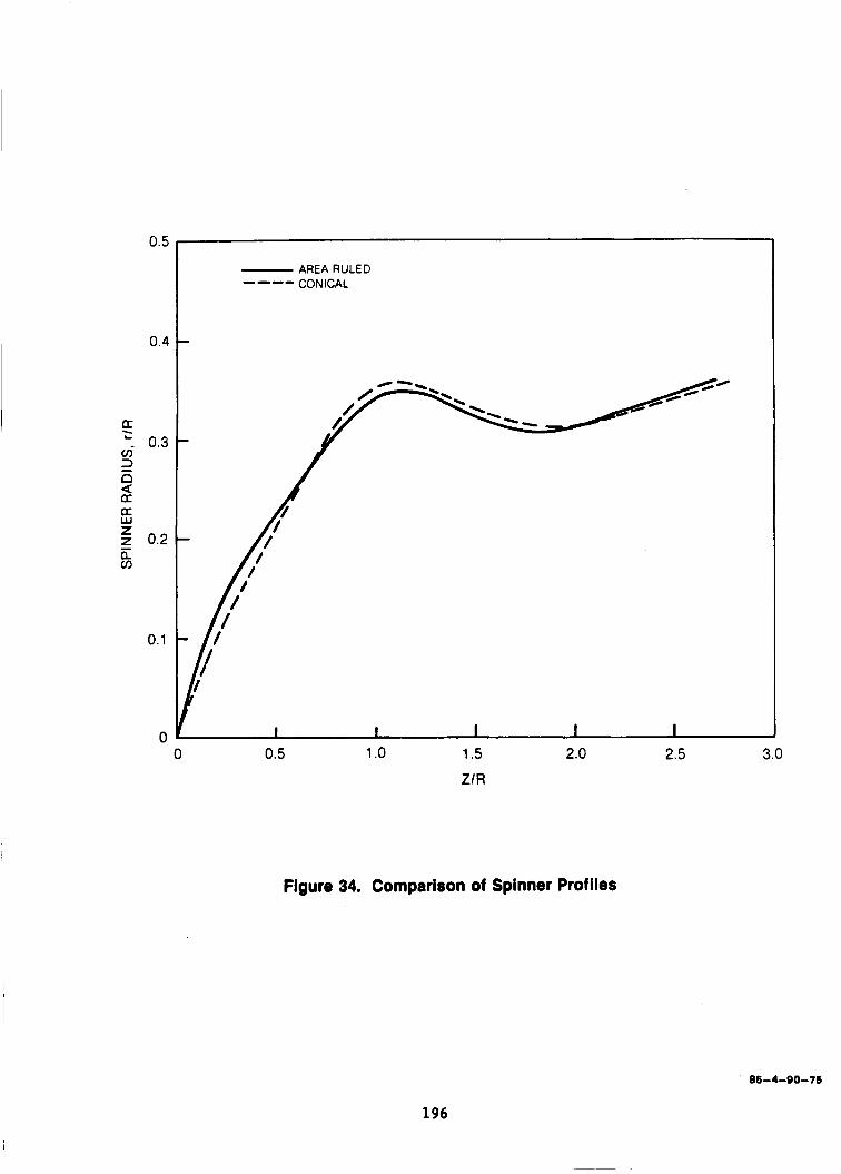
0.5

0.4

E m- 1 n

a

E

0.3

d

$ 0.2 w

0

0.1

0

- AREA RULED CONICAL ----

I I I I I 0 0.5 1 .o 1.5 2.0 2.5 3.0

Zl R

Figure 34. Comparison of Spinner Profiles

' 85-4-90-71

196

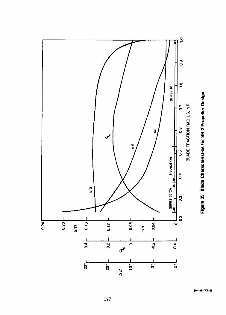
R 0

2 0

0

x 8 B I I I I

0 0 0 0 0 k N 0 g

Q

84-6-73-5

197

’ -

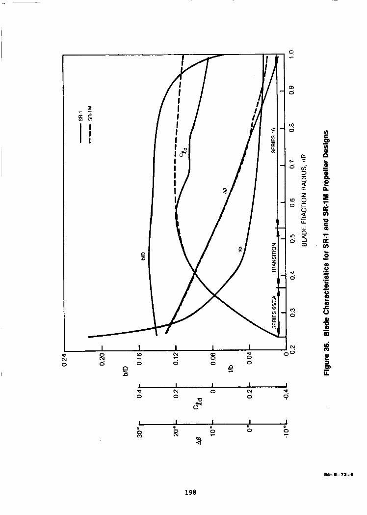
1 1 I 1 I

? B 0 2 s 0

I I I I I

8 I

0 0 0 0 0 0 (u

0 0 r

0 7

Qa 6

84-6-73-6

198

I I I I I n! 9

0

co w E 9 (D F 8 e o 0 9 0 0 - n

I I I I I n! 9

0

co w E 9

x 0 4 4

(D F 8 e o 0 9 0 0 - n

I I I I I Y 0 n! p:

jP I I I I I

nJ Q I - I

O 0 0 0 0 0 0 0 0

F

Q

I I I I I Y 0 n! p: x 0 4 4

jP

0 0 0 0 nJ Q I -

Q

0 0

0

0 F

84-6-73-7

199

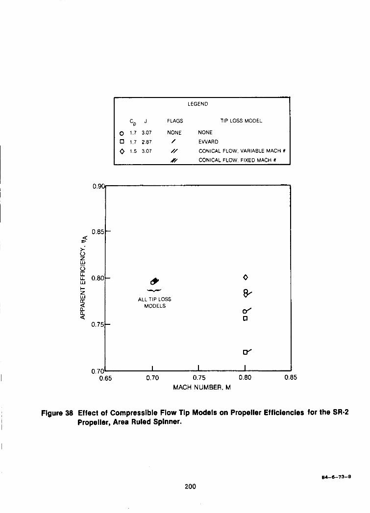
LEGEND

FLAGS TIP LOSS MODEL cP

0 1.7 3.07 NONE NONE

0 1.7 2.87 / EWARD

0 1 5 3.07 // CONICAL FLOW, VARIABLE MACH #

Ry/ CONICAL FLOW, FIXED MACH #

0.80

a i

w 0

c

0 Z

c I 2 W

n a U

2

5

ALL TIP LOSS MODELS

0

& d 0

O.7OL I I I 0.65 0.70 0.75 0.80 0.85

MACH NUMBER. M

Figure 38 Effect of Compressible Flow Tip Models on Propeller Efficiencies for the SR-2 Propeller, Area Ruled Spinner.

84-6-73-8

200

0.90

0.85 a i

w 0 E 0.80

f

2

W c Z W E Q a ' 0.75

0 1.7 3.07 NONE NONE a 1.7 2.87 / EVVARD

0 1.5 3.07 // CONICAL FLOW, VARIABLE MACH U /// CONICAL FLOW. FIXED MACH Cy

ALL TIP LOSS MODELS

0

w

ef

d

I I I 0.70

MACH NUMBER, M

Figure 39 Effect of Compressible Flow l i p Loss Models on Propeller Efficiencies for the SR4 Propeller, Area Ruled Spinner.

84-673-0

201

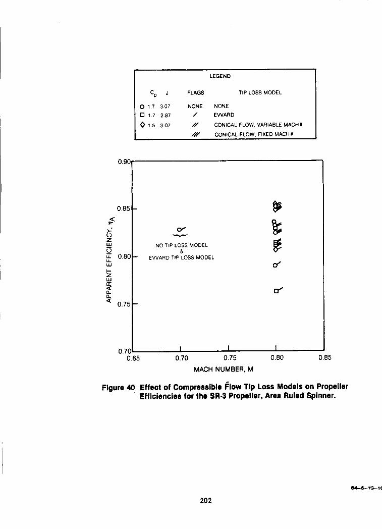
0.9c

0.85

a E

i 0 z w 0 Z 0.8C LL w I- z W 0: a a a 0.75

a

0.7( C

2

LEGEND

o/ - NO TIP LOSS MODEL

8 - EVVARD TIP LOSS MODEL d

d

I I I 5 0.70 0.75 0.80 0.85

MACH NUMBER, M

Figure 40 Effect of Compressible flow Tip Loss Models on Propeller Efficiencies for the SR-3 Propeller, Area Ruled Spinner.

84-6-73-1(

20 2

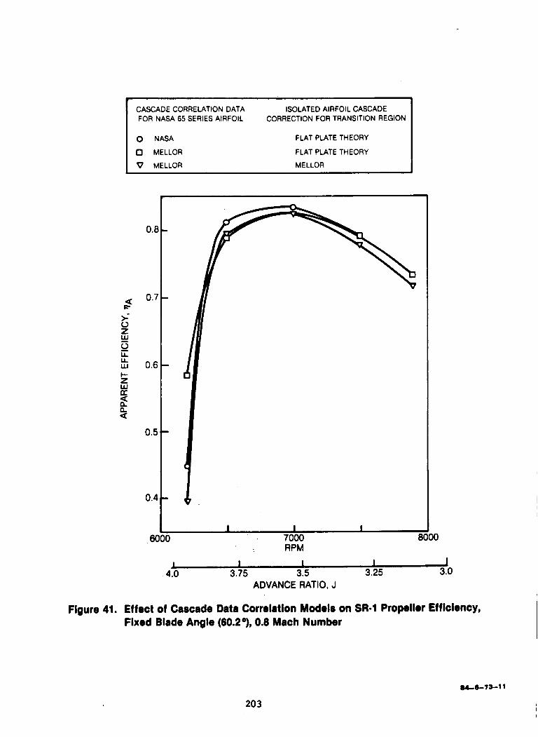
CASCADE CORRELATION DATA FOR NASA 65 SERIES AIRFOIL

0 NASA FLAT PLATE THEORY

0 MELLOR FLAT PLATE THEORY

V MELLOR MELLOR

ISOLATED AIRFOIL CASCADE CORRECTION FOR TRANSITION REGION

U t i

0

0 E U U w c z w 2 2 n

0.8

0.7

0.6

0.5

0.4

I I I 7000 8( RPM

6000 IO

.J I I I 1 4.0 3.75 3.5 3.25 3.0

ADVANCE RATIO, J

Figure 41. Effect of Cascade Data Correlation Models on SR4 Propellor Efficiency, Fixed Blade Angle (60.2O), 0.8 Mach Number

M-6-13-11

203

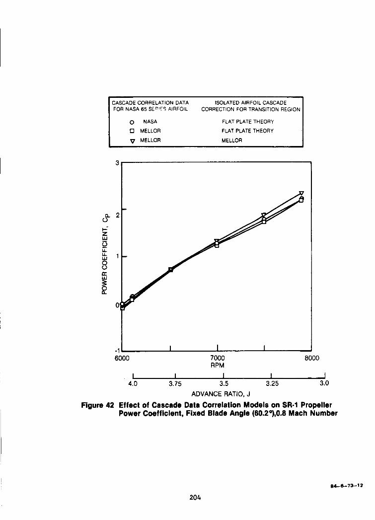
CASCADE CORRELATION DATA FOR NASA 65 SEE!:? AIRFOIL




v MELLOR MELLOR

6000 7000 RPM

8000

4.0 3.75 3.5 3.25 3.0 ADVANCE RATIO, J

Figure 42 Effect of Cascade Data Correlation Models on SR-1 Propeller Power Coefficient, Fixed Blade Angle (60.2O),0.8 Mach Number

84-673-12

204

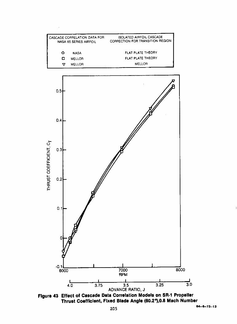
CASCADE CORRELATION DATA FOR NASA 65 SERIES AIRFOIL




V MELLOR MELLOR 1

0.5

0.4

0.:

0.;

0. '

(

-0: 6

I I 1 7000 E RPM

0

1 I 1 1 I 4.0 3.75 3.5 3.25 3.0

ADVANCE RATIO, J Figure 43 Effect of Cascade Data Correlation Models on SR-1 Propeller

Thrust Coefficient, Fixed Blade Angle (60.2'),0.8 Mach Number 84-6-73-13 205

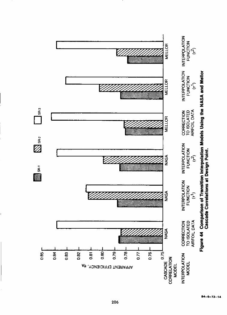
I In U 1 1 W I

c a

0 I

u v)

3 a z

3 a z

(D

0 ”.

z

84-6-73-14

206

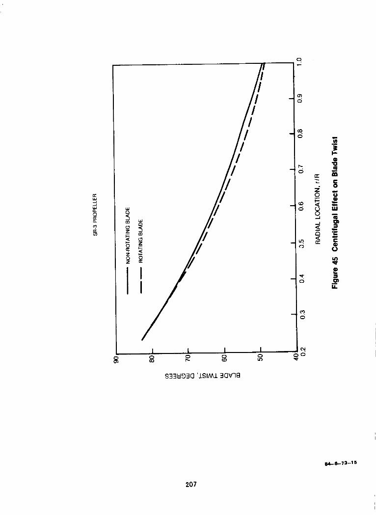
a

n

W -.I -J w

8 a a

(I)

I I I I 3 0 8 P (D

20 7

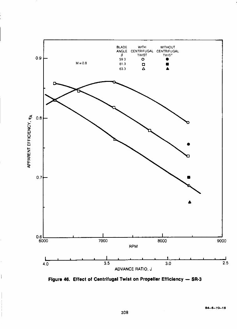
0.9

4 0.8 i 0 z w 0 U U w + z w

II z n a

0.7

0.6 6(

M = 0.0

BLADE WITH WITHOUT ANGLE CENTRIFUGAL CENTRIFUGAL s TWIST TWIST 59 3 0 0 61 3 0 m 63 3 A A

A

I I 1 I 1

RPM 10 7000 8000 9000

I I 1 1 I I I I I I I 1 1 I 1 I 4.0 3.5 3.0 2.5

ADVANCE RATIO, J

Figure 46. Effect of Centrifugal Twist on Propeller Efficiency - SR-3

208 84-6-73-16

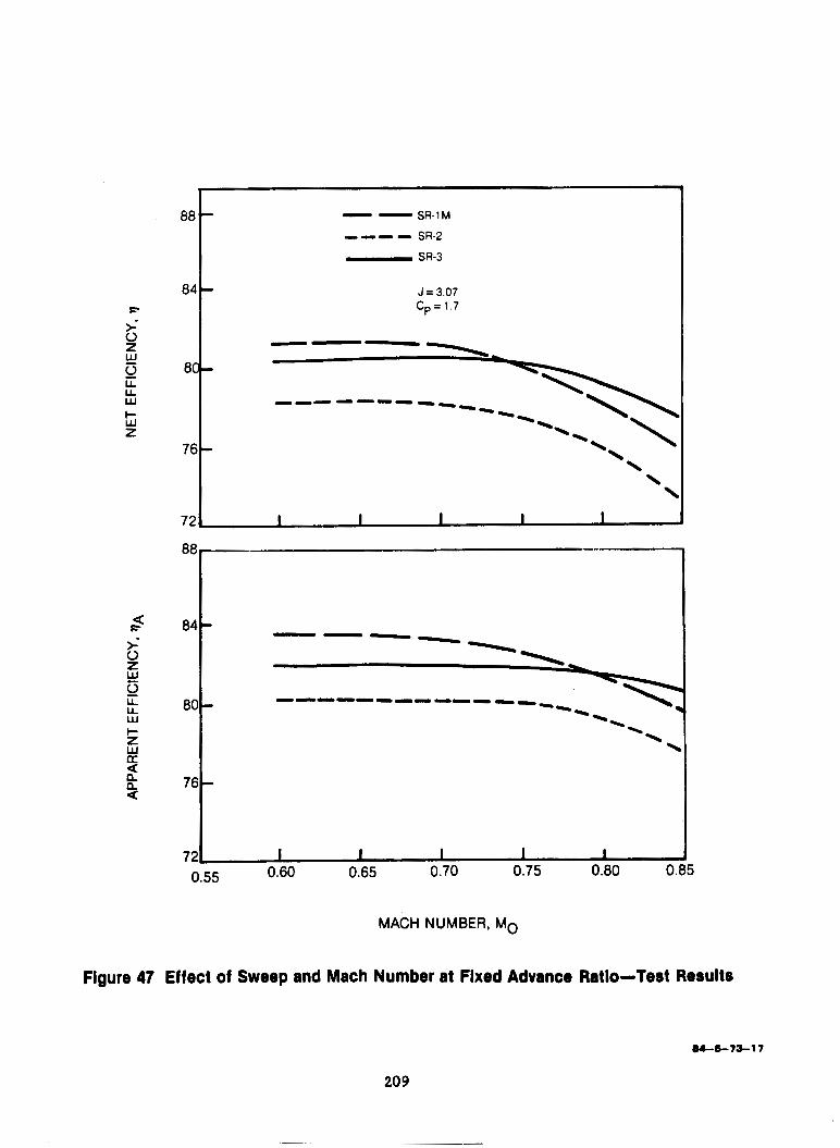
08

0r E i 0 z w 0 81 LL U W I- W z

7;

0E

s

0 U U 8(

0

5 W I- z w a a n n a 7t

7:

J = 3.07 C p = 1 . 7

\ \

I I I I I

I I I I I 0.60 0.65 0.70 0.75 0.80 0.85

0.55

MACH NUMBER, Mo

Figure 47 Effect of Sweep and Mach Number at Fixed Advance Ratio-lest Results

B4-6-73-17

209

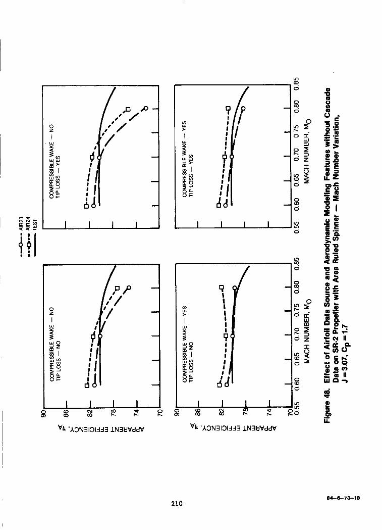
vb 'A3N3131dd3 lN3UVddV vb 'A3N3131dd3 lN3UVddV

84-8-73-18 210

vh ‘A3N3131dd3 lN3kiVddV vh ‘A3N3131dd3 lN3kiVddV

04-6-73-19

211

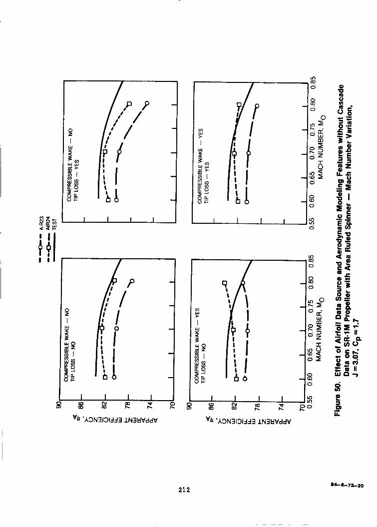
' h 'A3N3131dd3 lN3tlVddV

I I I I In lv! 00 8 % E h h

' h 'A3N3131dd3 lN3tJVddV

21 2

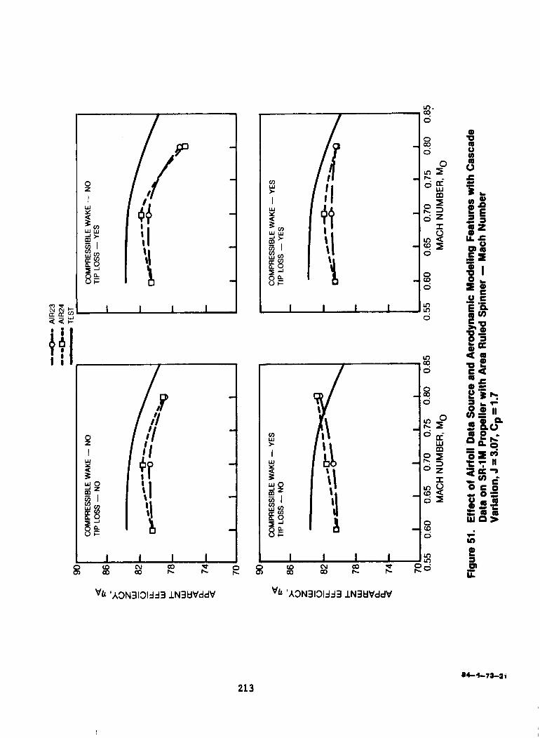
vh ‘A3N3131dd3 lN3UVddV

844-73-21

213

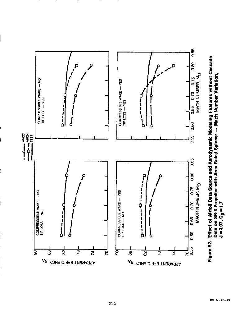
rn ?

L n

v& 'A3N3131J33 lN3UVddV

214 844-73-22

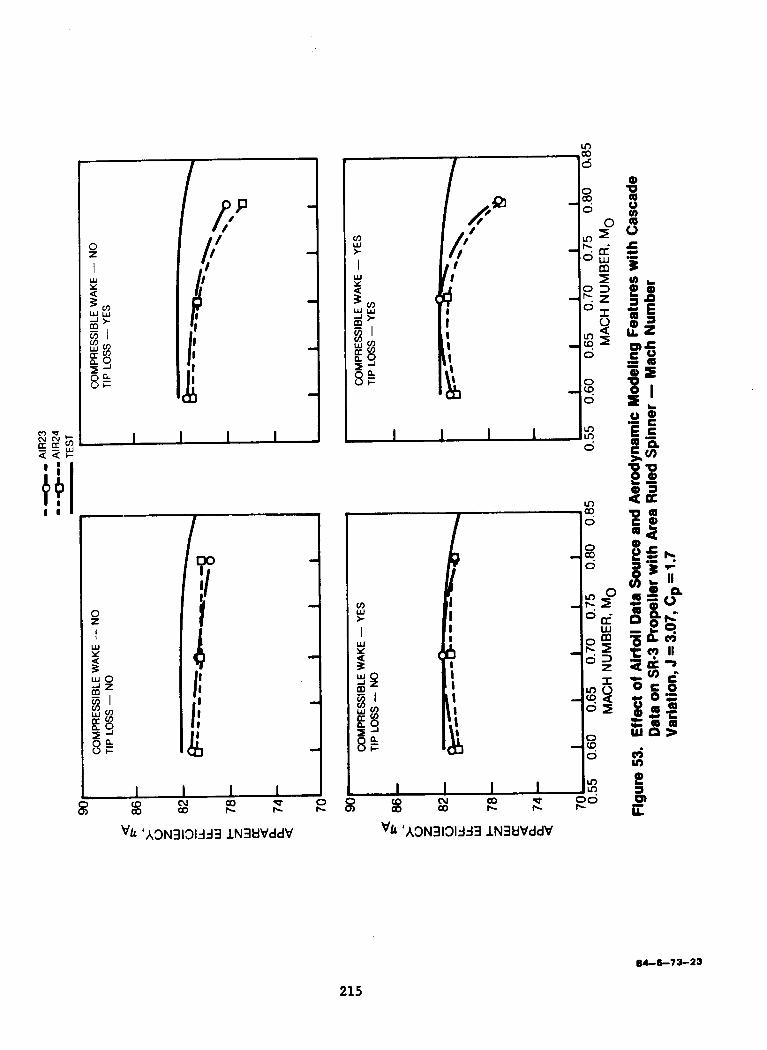
vh 'A3N3131333 lN3UVddV vh 'A3N3131dd3 lN3UVddV

64-6-13-23

215

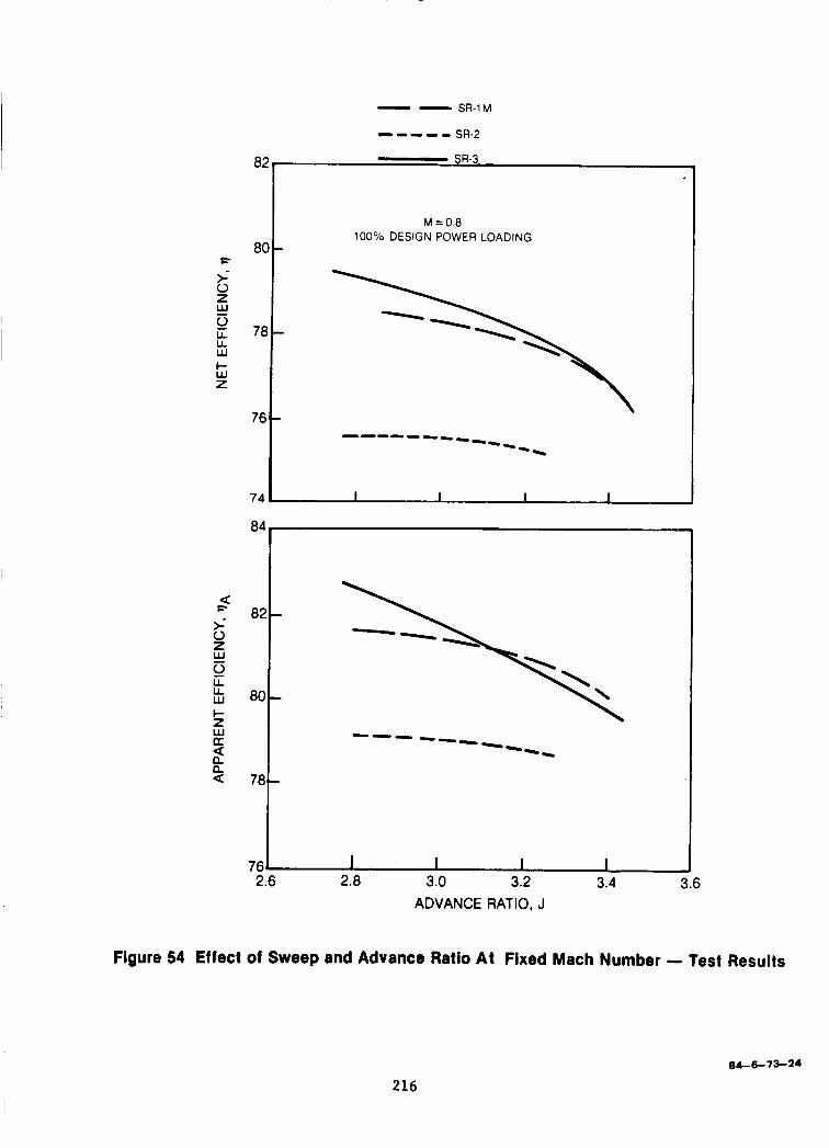
F

i

0

0

5 U U W I- W z

a s

0

e

0

5

3 a a

U U W I-

a a U

82

8C

78

76

74

M = 0.8 100% DESIGN POWER LOADING

-- -------- --- I I I I

ADVANCE RATIO, J

Figure 54 Effect of Sweep and Advance Ratio At Fixed Mach Number - Test Results

84-6-73-24

216

84

82 - a i = 80- w

e

0

0 LL - -m

L L

I-

w

w 78- z D------- a 2 76- % -\

74 1 I I

COMPRESSIBLE WAKE - YES TIP LOSS - NO

80 - 78 -

76 - -a a" - - -O- - -

74 - 72 - o-w--

70 I I I I

COMPRESSIBLE WAKE - YES 84, TIP LOSS - YES

76 2.6 2.8 3.0 3.2 3.4 3.6 2.6 2.8 3.0 3.2 3.4 3.6

ADVANCE RATIO, J ADVANCE RATIO, J

Figure 55. Effect of Airfoil Data Source and Aerodynamic Modeling Features without Cascade Data on SR-2 Propeller with Area Ruled Spinner - Advance Ratio Variation, M rO.8, 100% Design Power Loading

OC6-73-26

21 7

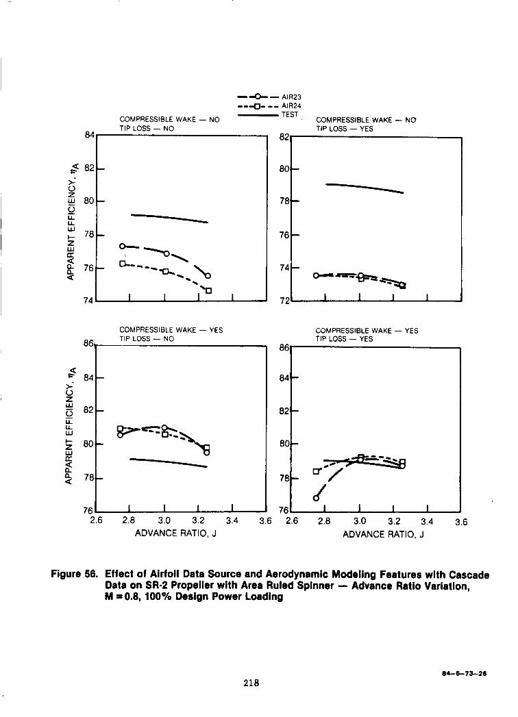
-+ - AIR23

COMPRESSIBLE WAKE - NO TEST COMPRESSIBLE WAKE - NO

--e -- AIR24

TIP LOSS - NO TIP LOSS - YES 84

3 82- i 0

5 80- I!

t- 78-

a a a

LL IL w

Z w

74 I I 72

76- \

'0

86

84

82

80

78

76


-

- - -

1 I I

a 7 84 > 0

82 0

I- 80

LL LL w

5 a a

a a a 78

c

76 - 2.6 2.8 3.0 3.2 3.4 3.6 2.6 2.8 3.0 3.2 3.4 3.6


I Figure 56. Effect of Airfoil Data Source and Aerodynamic Modeling Features with Cascade Data on SR-2 Propeller with Area Ruled Spinner - Advance Ratio Variation, M =0.8, 100°/~ Design Power Loading

218 84-6-73-26

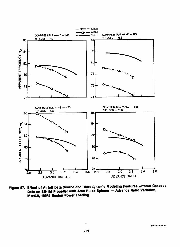
-e- AIR23 --e - 0 AIR24

COMPRESSIBLE WAKE - NO - TEST COMPRESSIBLE WAKE - NO TIP LOSS - NO TIP LOSS - YES

84 i

76 1

I I 76 I

7 6 1

8 6 ~

84 s-

s2

I- 80

o z

821 U LL W

5 U

4 i$ 78-

COMPRESSIBLE WAKE - YES 86, TIP LOSS - YES -. .. .

\ - ‘*s

b .. \

b I- -- 78


Figure 57. Effect of Airfoil Data Source and Aerodynamic Modeling Features without Cascade Data on SR-1M Propeller with Area Ruled Spinner - Advance Ratio Variation, M -0.8, 100% Design Power Loading

-

219

04-673-27

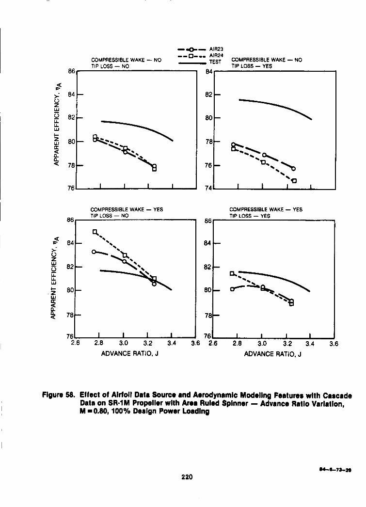
-e- AIR23 - - m--- AIR24 COMPRESSIBLE WAKE - NO - TEST COMPRESSIBLE WAKE - NO TIP LOSS - NO TIP LOSS - YES

Y w LL LL w c

a U Q

78

76

COMPRESSIBLE WAKE - YES

U c >- 0 z w 0 LL LL w c z w U Q a

%

78

76

74 1 I I I I

COMPRESSIBLE WAKE - YES 8 ~ , TIP LOSS - YES

84

78t 2.6 2.8 3.0 3.2 3.4 3.6 2.6 2.8 3.0 3.2 3.4 3.6


Figure 58. Effect of Airfoil Data Source and Aerodynamic Modeling Features with Cascade Data on SR4M Propeller with Area Ruled Spinner - Advance Ratio Variation, M = 0.80, 100% Design Power Loadlng

220

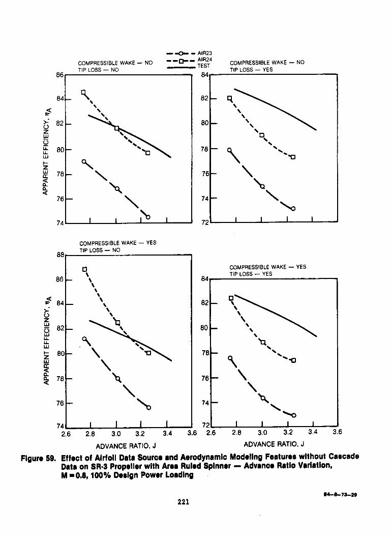
-e* COMPRESSIBLE WAKE - NO -om-

R6. - TIP LOSS - NO

7 4 1 1


881

7 2 2

82

80 8- 78

82

80

78

76

74 76

-

'

I

8

I

'. 9

\

\

- AIR23 . AIR24 .. TEST COMPRESSIBLE WAKE - NO 8rl TIP LOSS - YES

82

78 8ot q\\ \ 0

'\

COMPRESSIBLE WAKE - YES TIP LOSS - YES

- \ \

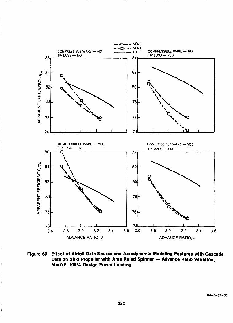
-+- 0 -0- -.

COMPRESSIBLE WAKE - NO TIP LOSS - NO


AIR23 AIR24 TEST COMPRESSIBLE WAKE - NO 84, TIP LOSS - YES ,

COMPRESSIBLE WAKE - YES ~~, TIP LOSS - YES

761 I *d 7 4 d 2.6 2.8 3.0 3.2 3.4 3.6 2.6 2.8 3.0 3.2 3.4 3.6


Figure 60. Effect of Airfoil Data Source and Aerodynamic Modeling Features with Cascade Data on SR4 Propeller with Area Ruied Spinner - Advance Ratio Variation, M =0.8, 100°/~ Design Power Loading

84-6-73--30

222

f

i

0

0 P L L LL W I- W z

a i 0 z w 0

P

LL LL W I- z W [I

0 a 2

80.

78

76

74

M = 0.8 100% DESIGN POWER LOADING

1 -----\

- -1

-

J I 1 1 1

2.6 2.8 3.0 3.2 3.4 ADVANCE RATIO, J

3.6

Figure 61. Effect of Twist and Area Ruling - Test Results

223

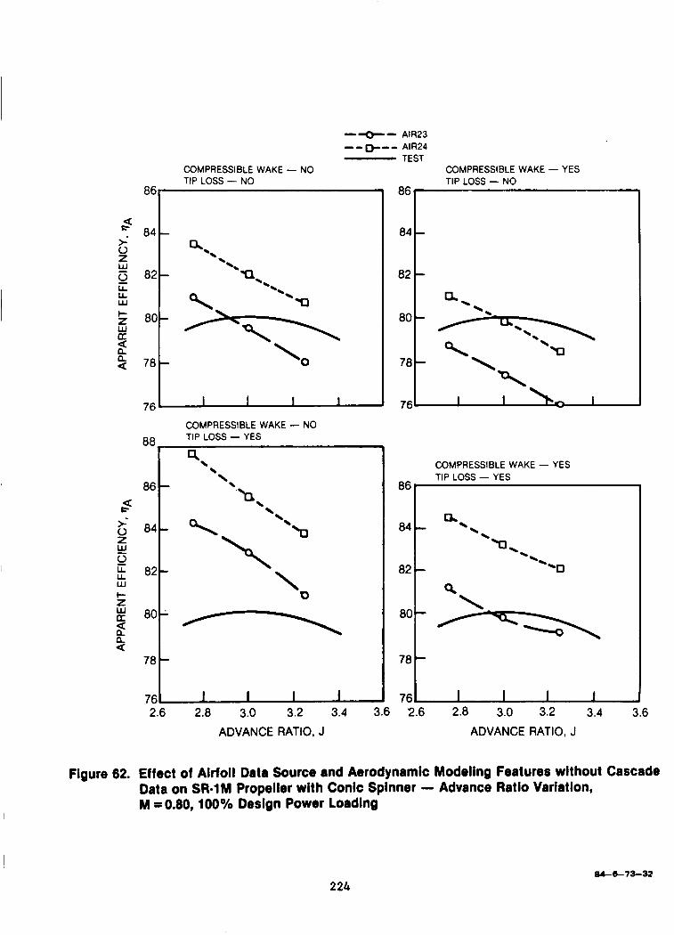
86-

a e 84- >- &

II .. --. 0 z -. 82-

n --. U U w \ 5 80-

2 78-

w a \\ \o

a n

I 1 I I 76

88

86 a e

86

84 -

82 - -.- m.

\

80 - Yl

\

- 76 I I n I

78 - \

-

&- 84 z w 0

82 w I- z g 8C a 2 n

80-

78

76

78

7E

Q \-

/-L

- - I I I I

COMPRESSIBLE WAKE - NO TIP LOSS - YES

D \

COMPRESSIBLE WAKE - YES TIP LOSS - YES

2.6 2.8 3.0 3.2 3.4 3.6 2.6 2.8 3.0 3.2 3.4 3.6 ADVANCE RATIO, J ADVANCE RATIO, J

Figure 62. Effect of Airfoil Data Source and Aerodynamic Modeling Features without Cascade Data on SR-1M Propeller with Conic Spinner - Advance Ratio Variation, M =0.80, 100°/~ Design Power Loading 1

224 84-6-73-32

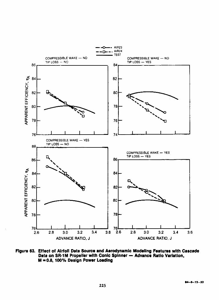
86 , 84

$5 84- 82 i

80

LL w

78

U a 78- 76

Q

I I I 1 76 74 COMPRESSIBLE. WAKE - YES

8a8

- - F\ '' \ -

--+o \

n '\ - I I I I

76 1,1111

86-

84

82

80-

78

76

- 9

- & -3\

/ = \

- I I I I -

2.6 2.8 3.0 3.2 3.4 3.6 2.6 2.8 3.0 3.2 3.4 3.6 ADVANCE RATIO, J ADVANCE RATIO, J

Figure 63. Effect of Airfoil Data Source and Aorodynrmic Modoling Featuns with Cascade Data on SR-1M Propeller with Conic Spinnor - Advrnco Ratio Variation, M m0.8, 100% Design Powor Loading

225 04-673-33

\ 0

5 76- w a U 0 n 74- U

L L U w

b \

I 1 1 1 72C

'0 \. 76 -

\ 74 -

b 72 - 70 I 1 I 1

6

84

9 \ \

\ 4 82- \

$ \ \

0

% 5 80.- 0

+ 78- a

L L w z w \

\ 3

74 I I 1 1 I

\ 2 76-

Figure 64. Effect of Airfoll Data Source and Aerodynamic Modeling Features without Cascade Data on SR-1 Propeller with Conic Spinner - Advance Ratio Variation, M = 0.8,100% Design Power Loading

82

\ 9

80 - \ 78 - -73 "\

\ 76 -

\ 74 - \ 72 I I I I

04-6--73--34

226

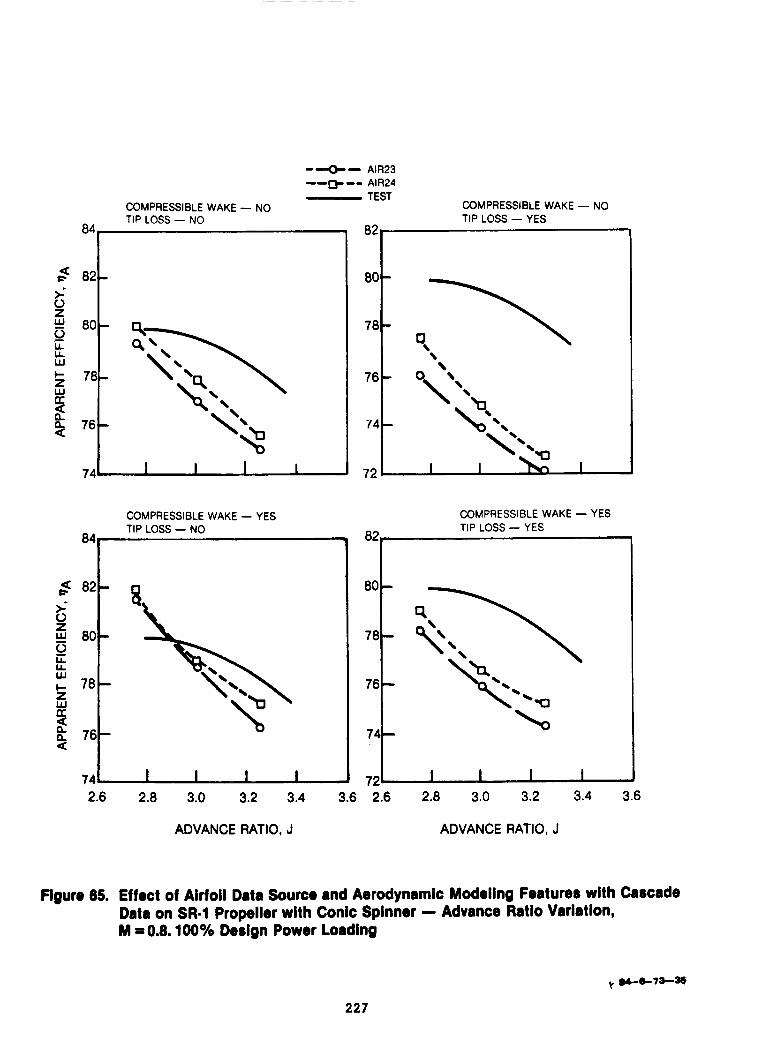
-e- AIR23 --m-- AIR24

TEST COMPRESSIBLE WAKE - NO COMPRESSIBLE WAKE - NO

82, TIP LOSS - YES

3 82

82

78-

80

76

74

727

76

74

9;. -

-

- I I I I

. \

0,'. \

74 721 I I I

COMPRESSIBLE WAKE - YES 84s

7 4 4 2.6 2.8 3.0 3.2 3.4 3.6 2.6 2.8 3.0 3.2 3.4 3.6


Figure 65. Effect of Airfoil Data Source and Aerodynamic Modeling Features with Cascade Data on SR-1 Propeller with Conic Spinner - Advance Ratio Variation, M = 0.8.100% Design Power Loading

227

/

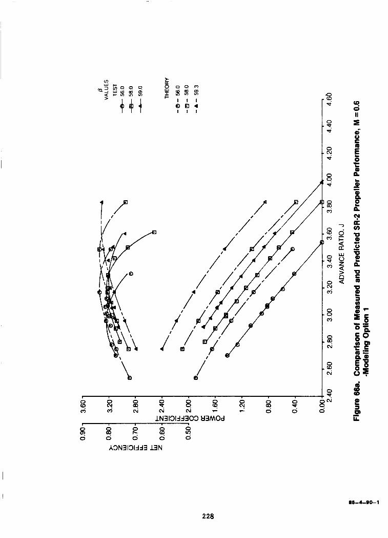
0 (D

06-440-1

228

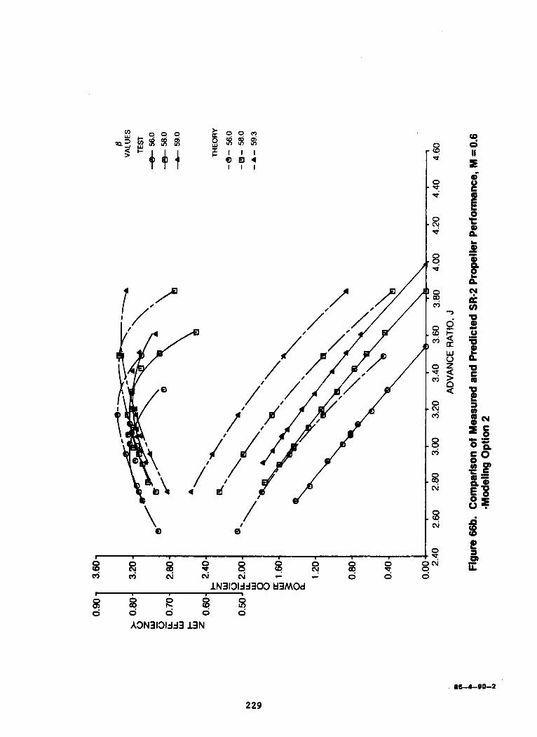
0

w s

0

d c\!

0

2

0 z

229

/ ,/'

0 r m

0

' %

-2 0

85-4-00-3,

230

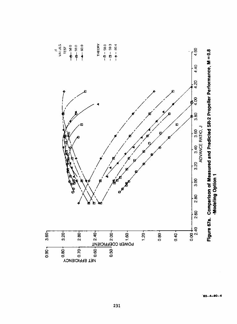
0 0 8"' 0 x 0 c9 0

c\! .- 8 F

8 0 0 0 0 2 x z 2 c\i

lN3131dd303 tl3MOd 0 0 0 0 c9 0 2 2 F

A3N3131dd3 13N 0

8 0

'86-4-00-4

231

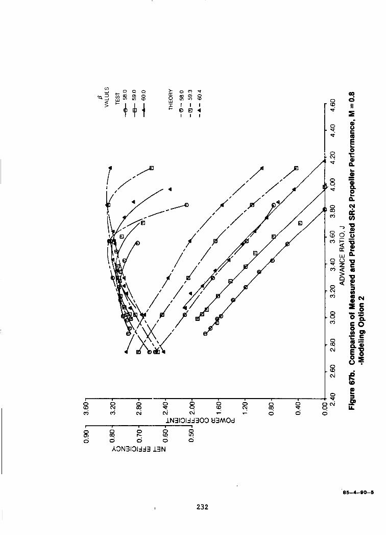
t I

0 0 0 0 0 0 0 0 0

2 x 2 2 z F 2 x 8 n! 7

(9

0 0 0 0 v! 0

2 2 0 2 0 r-

I 232

t

0 0 0 0 , s I 0

aq 0

c\! F

(9 F

a 0 0 0 0 'p ni 2 x : cu I

lN3131dd303 kt3MOd t 1

5: 0 0 Y 0 0

A3N3131dd3 13N 0

8 8 0

16-4-90-6

233

A

r 10 -? o! O N = 0,

0 0 0 0 .a 0

N c9 l- 0

(9 8 i i l-

8 s 0 cu ni

2 2 2 0 0

0 0 0 0 s co N

c\!

lN313M3303 tJ3MOd I

0 8 0 0 0 rc A3N3131dd3 13N

86-4-90-18

234

I 0 0

0 s 8 0

2 ci x cj r 0 8 r

8 0 8 c j

8 lN3131dd303 U3MOd

8 0

53 0

0 0 rc

0

A3N3131dd3 13N

8 8 0

235

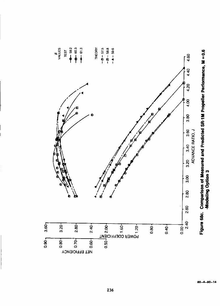
86-4-00-14

236

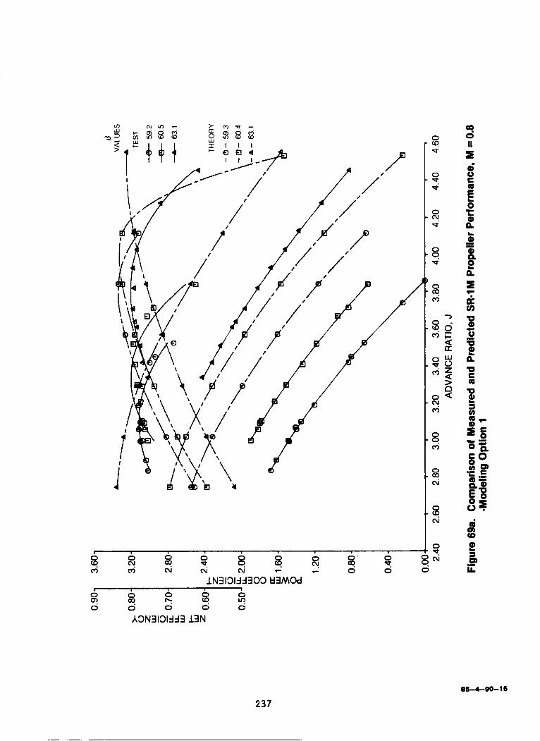
b c 0 8 0 0 0 0

Tt (4 2 0 r\! .- c

8 0 0 0 0

t-4 ac! Tt 2 x N N

lN313133303 U3MOd r 1 0 0 0 0 0 rc

0

A3N3131333 13N

0

2

0

2 0 z 0

2

0

N ac!

B t a v)

3 c 0

06-4-00-1 6

23 7

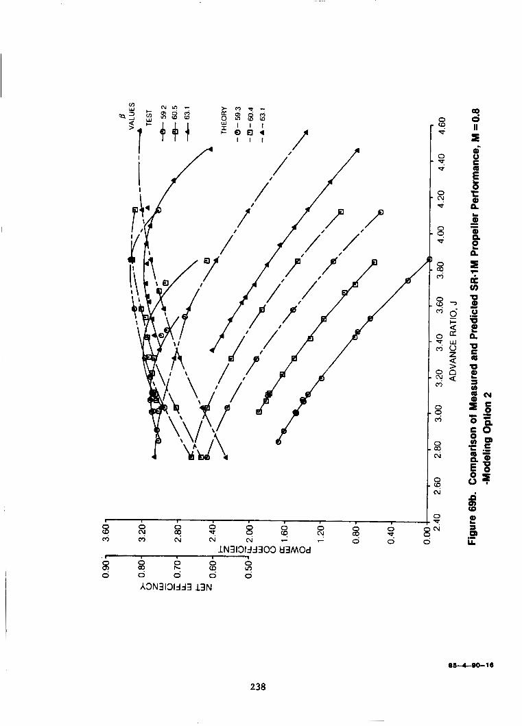
r 0 "1

0 0 0 O W N m 0 0 0 0 0 0 (9 .- 2 0 8 LL

s 7 2 m z c

2 0 0 0

ct (v

c9 (v

9

I N 3 131dd 303 tJ3MOd r I

0 0 0 0 0 c9

A3N3131dd3 1 3 N

I

2 Y (9

86-4-00-16

238

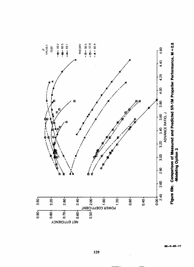
86-4-80-1 7

239

f /

Q

/ P

t 0 f 2 x : x : ?

0 0 0 0 . Ax .- LL 0

-? 0

8 0 0 0 0 0 e F 0

(4

lN3131dd303 tl3MOd t I

0 0 0

0 0 0 v! (4 rc

A3N3131dd3 13N

8 0

8 0

85-4-90-12

240

~&-c-SO-lO

241

/

85-4--90-8

24 2

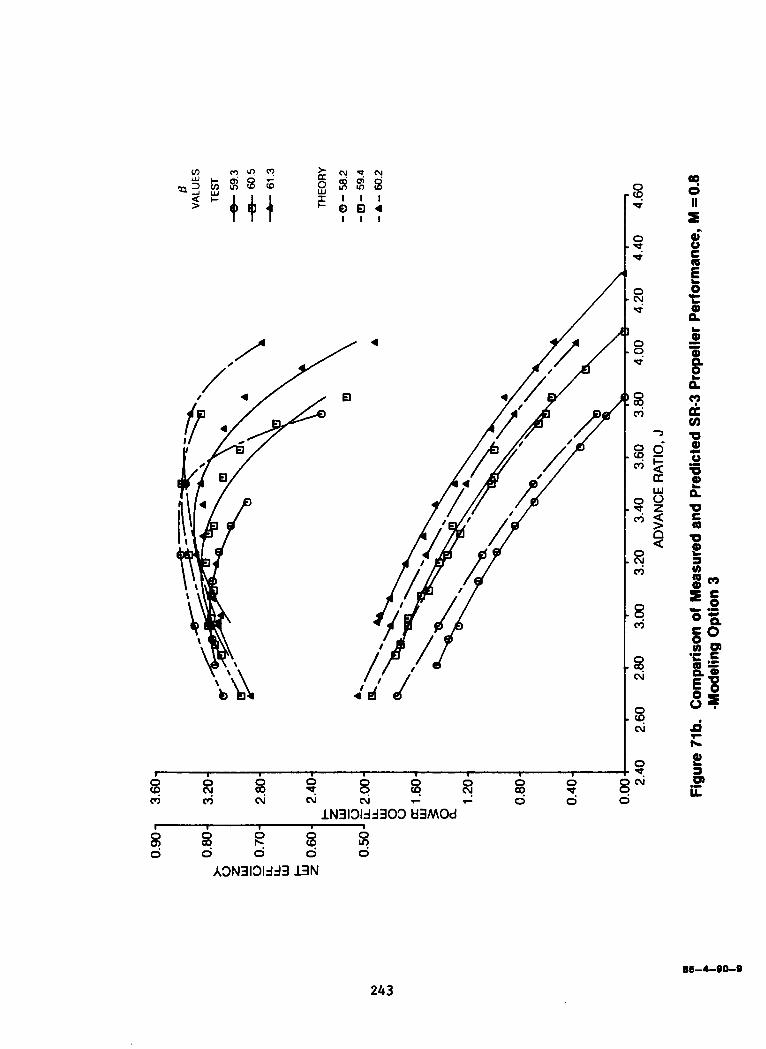
lN3131dd303 ti3MOd 1 I

0

2 fi 0 0

0

A3N3131dd3 13N

k 8 0 ii 0

243

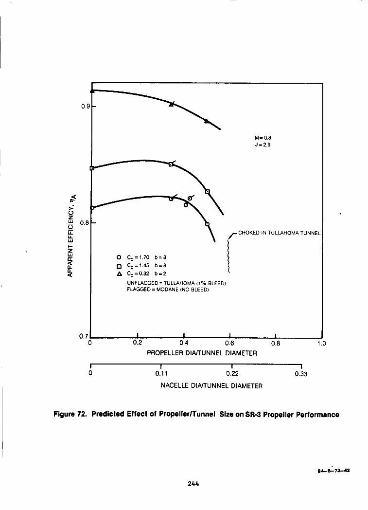
O.!

U r i 0 Z E 0.E 0 L L LL w c 5

2 a 4: 0

0.7

0 a A

M= 0.8 J = 2.9

I Cp = 1.70 b = 8 Cp= 1.45 b =8 Cp =0.32 b = 2

UNFLAGGED = TULLAHOMA (1 '10 BLEED) FLAGGED = MODANE (NO BLEED)

I 1 I I

0.2 0.4 0.6 0.8 1 .o PROPELLER DlAlTUNNEL DIAMETER

I 0.1 1

I

0.22 I

0.33

NACELLE DlAlTUNNEL DIAMETER

Figure 72. Predicted Effect of PropellerlTunnel Size on SR.3 Propeller Performance

244

~ ~~~

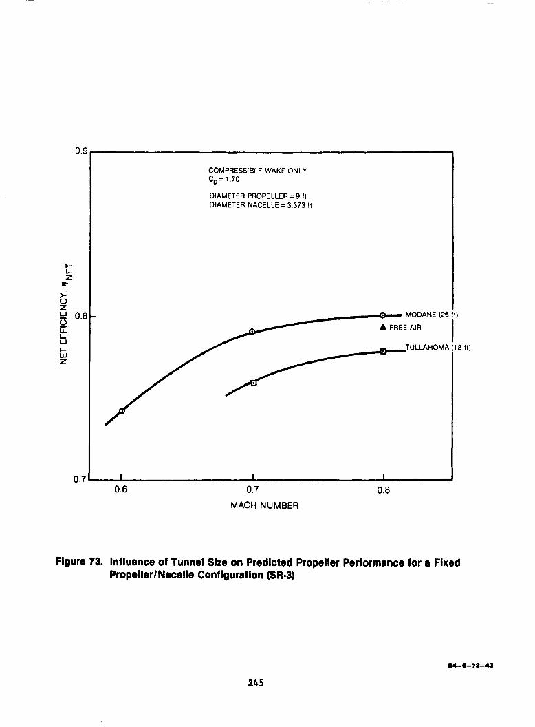
COMPRESSl6LE WAKE ONLY Cp = 1.70

DIAMETER PROPELLER = 9 i t DIAMETER NACELLE = 3.373 f t

A FREE AIR

I . I I

0.6 0.7 0.8 MACH NUMBER

1)

18 1 1 )

Figure 73. influence of Tunnel Site on Predicted Propeller Performance for a Fixed Propeller/ Nacelle Configuration (SR-3)

245

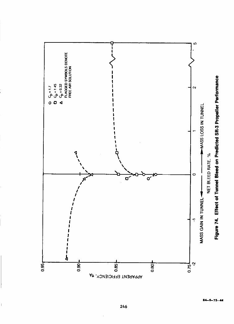
I I I I I I I I I I I

4 \ \

/ / I

I I I I I I I I I I I I I

I I I In 0

09 0

09 0

b 8 0

84-6-7344

246

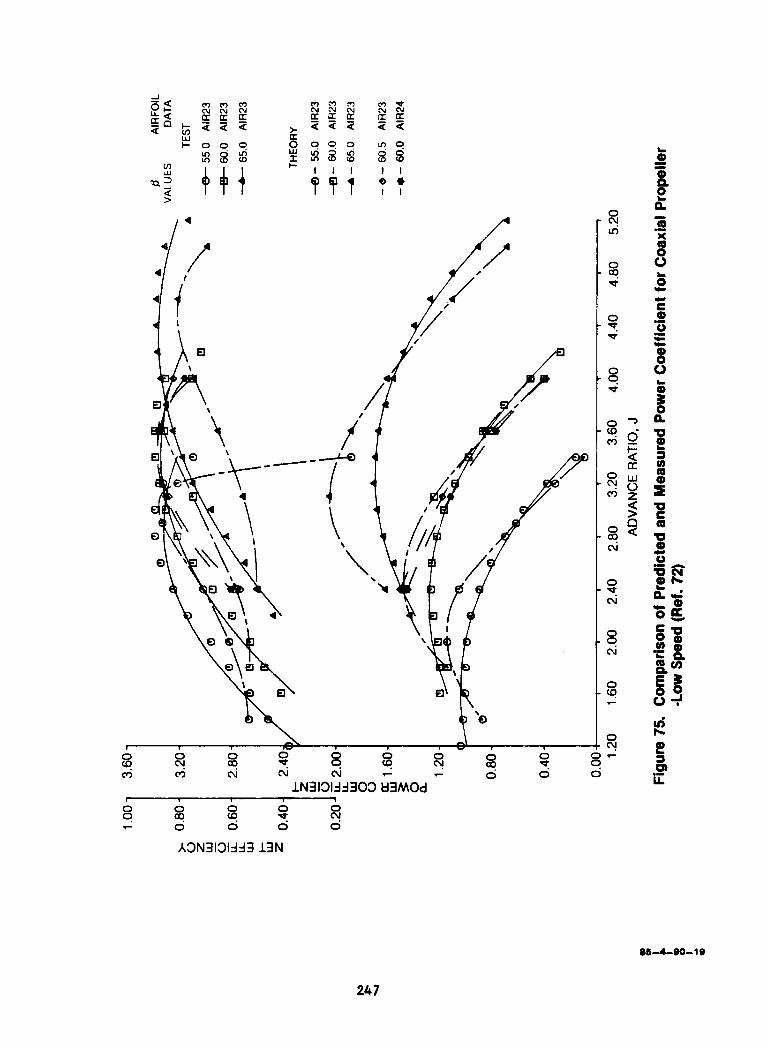
d I- O

h! 0 0 0 07 h! f

CR LL .- 9

0 s g 0 7

8 7

8 0 0 0 0

2 x 2 x cj lN31313d303 tl3MOd

0 0 0 0

A3N3131JJ3 13N

2 s 2 2 0 8 7

86-4-90-19

24 7

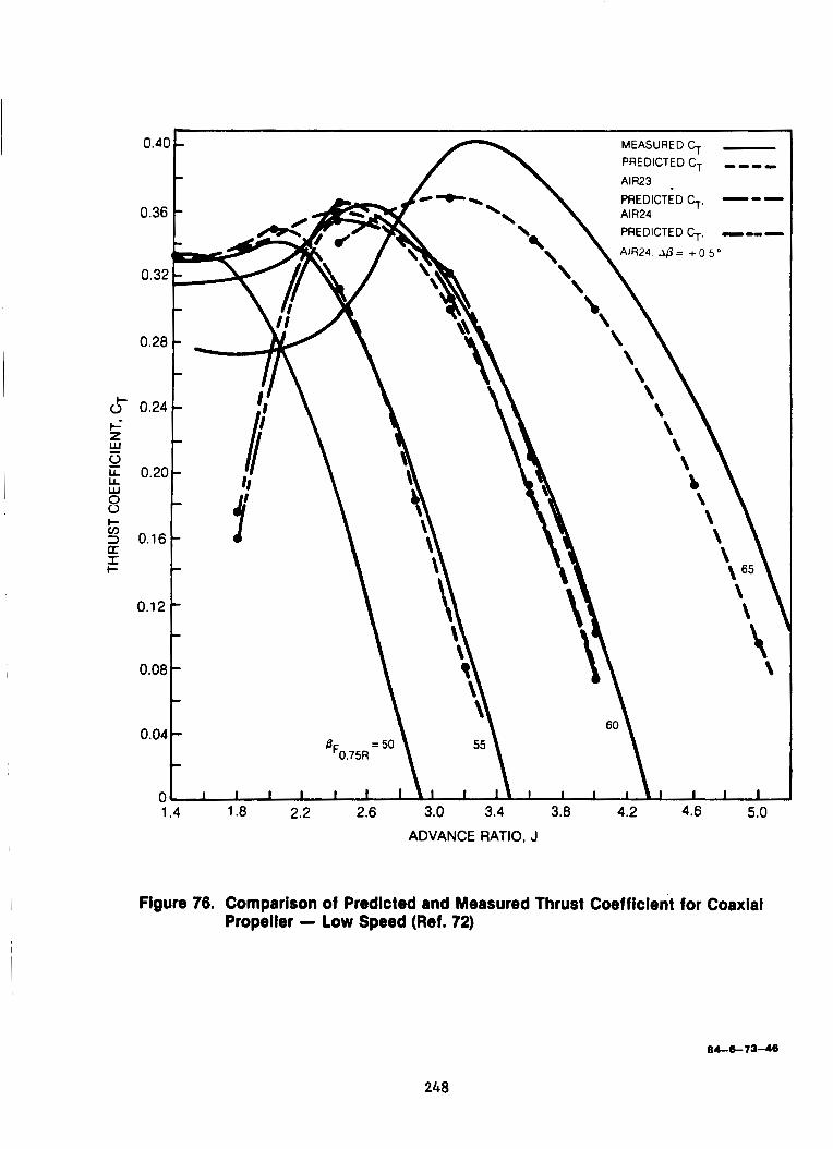
ADVANCE RATIO, J

Figure 76. Comparison of Predicted and Measured Thrust Coefficient for Coaxial Propeller - Low Speed (Ref. 72)

64-6- 7 3-46

248

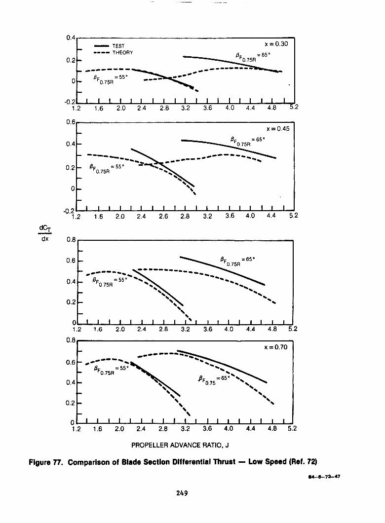
0.4 x = 0.30 - - TEST

0--- THEORY

0.2 - c I I I I - - -

0- BF0,75A= 55"

c

x = 0.45 0.6

L

-0.21 I I I I I I I I I I I I I I I I I I 1.2 1.6 2.0 2.4 2.6 2.8 3.2 3.6 4.0 4.4 5.2

1 1 1 1 1 1 ' 1 1 1.2 1.6 2.0 2.4 2.8 3.2 3.6 4.0 4.4 4.8 f 2

x=0.70 I 0.8 1

PROPELLER ADVANCE RATIO, J

Figure 77. Comparison of Blade Section Differential Thrust - Low Speed (Ref. 72)

04-6-73-47

249

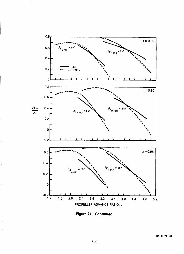
0.8

0.6

0.4

0.2

\

t --.. - - - c~------- BFO 75R = 550 0 - \\= o'80

- - '. - TEST

8 \ \ '8 '. ---- THEORY \ - L

8 '.

\ '. : j 0

8

' '.

-8

1 1 1 1 1 1 1 1 ~ I 1 1 1 1 1 1 1 1 1 8.

1.2 1.6 2.0 2.4 2.8 3.2 3.6 4.0 4.4 4.8 5.2 -0.2

PROPELLER ADVANCE RATIO, J

Figure 77. Continued

84-6-73-48

250

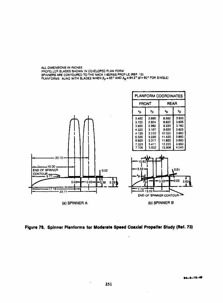
ALL DIMENSIONS IN INCHES PROPELLER BLADES SHOWN IN DEVELOPED PLAN FORM SPINNERS ARE CONTOURED TO THE NACA 1-SERIES PROFILE (REF. 12) PLANFORMS ALINE WITH BLADES WHEN BF = 65' AND 1 3 ~ = 64.2. ( B = 60. FOR SINGLE)

3.482 2.890 8.582 3.655 3.720 2.924 8.820 3.695 3.920 2.992 9.220 3.760 4.320 3.167 9.620 3.825 4.720 3.220 10.020 3.860 6.520 3.220 11.420 3.860 6.920 3.317 11.820 3.890 7.320 3.411 12.220 3.950 7.706 3.502 12.806 4.040

_I

(a) SPINNER A

1 PLANFORM COORDINATES

I FRONT I REAR

' END OF SPINNER CONTOURS

(b) SPINNER B

Figure 78. Spinner Planforms for Moderate S p e d Coaxial Propeller Study (Ref. 73)

25 1

1.06

1.04

1 .G2

1 .oo

0.98 V N O

0.96

0.94

0.92

0.90 0

\ 1 \ \ \

I I I I 0.2 0.4 0.6 0.8 1 .o

- - - FRONT TYPE B --OD- REAR TYPE B

/ /

/ I

/ I I I I I I

25 2

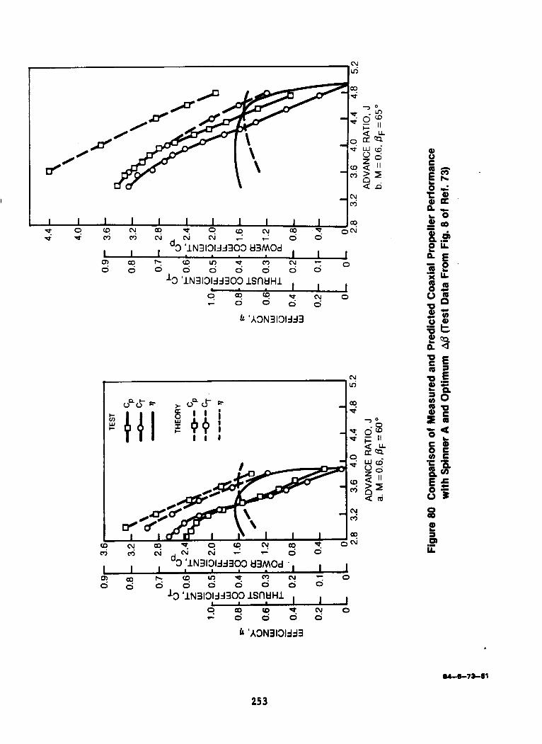
p/

d(’ 1”

253

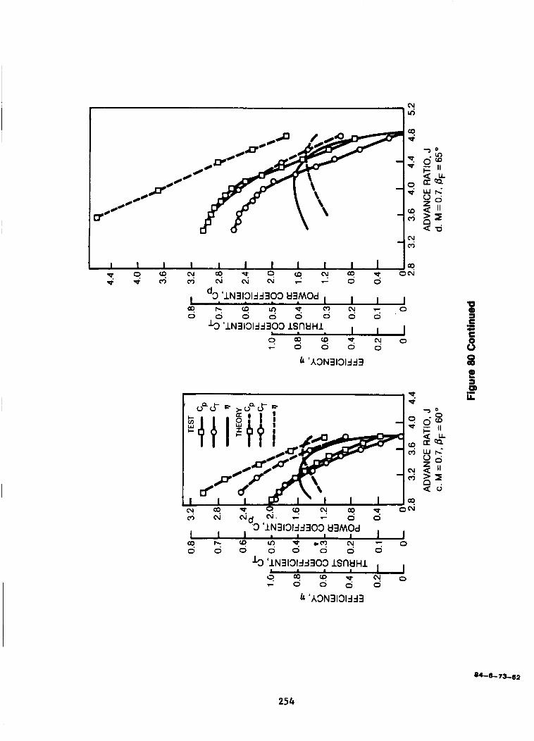
I 1 9

O d d s

254

O . ' t $- 0.6.

o"

w

W

TEST - 3.2

2.8 - -5 - v

2.8 3.2 3.6 4.0 4.4 ADVANCE RATIO, J e. M = 0.8, OF = 60"

2.8 3.2 3.6 4.0 4.4 4.8 5.2

ADVANCE RATIO, J 1. M = 0.8, = 65"

Figure 80 Concluded

255

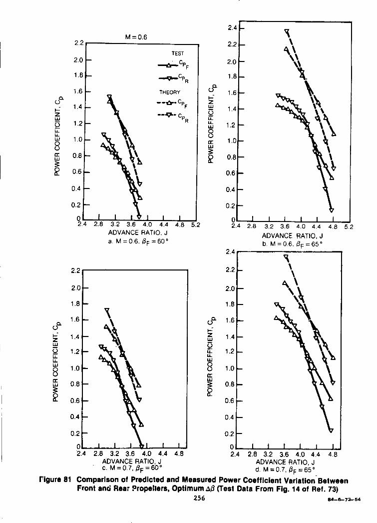
M = 0.6

2.2 I

2.0

1.8

1.6

1.4

1.2

1.0

0.8

0.6

0.4

0.2

1.8 *'O 1

- - - - - - - - - -

0" L t w 0 LL L L

8

ADVANCE RATIO, J a. M=0.6, P ~ = 6 0 "

2*2 1 1.8 2.0 t

0" I-- z w 0 LL LL

-

# U

8

2.4 2.8 3.2 3.6 -4.0 4.4 4.8 ADVANCE RATIO, J

. C. M=0.7, /3F=6Oo

0" I--

w 0 z

LL LL

8 0 a

E

P I--

0 E 8 LL L

0 a

E

0- 2.4 2.8 3.2 3.6 4.0 4.4 4.8

ADVANCE RATIO, J b. M = 0.6. Pr = 65

5.2

2.2 2.49\

0 s 2.4 2.8 3.2 3.6 4.0 4.4 4.8

ADVANCE RATIO, J d. M z 0 . 7 , f l ~ = 6 5 "

Figure 81 Comparison of Predicted and Measured Power Coefficient Variation-Between Front and Rea: Fropellers, Optimum AB (Test Data From Fig. 14 of Ref. 73)

256 64-6-73-54

0.4 t BF =

O*** 0 2.4 2.8 3.2 3.6 4.0 4.4 4.8 5.2

ADVANCE RATIO, J e. M=0.8

Figure 81 Concluded

84-6-73-65

25 7

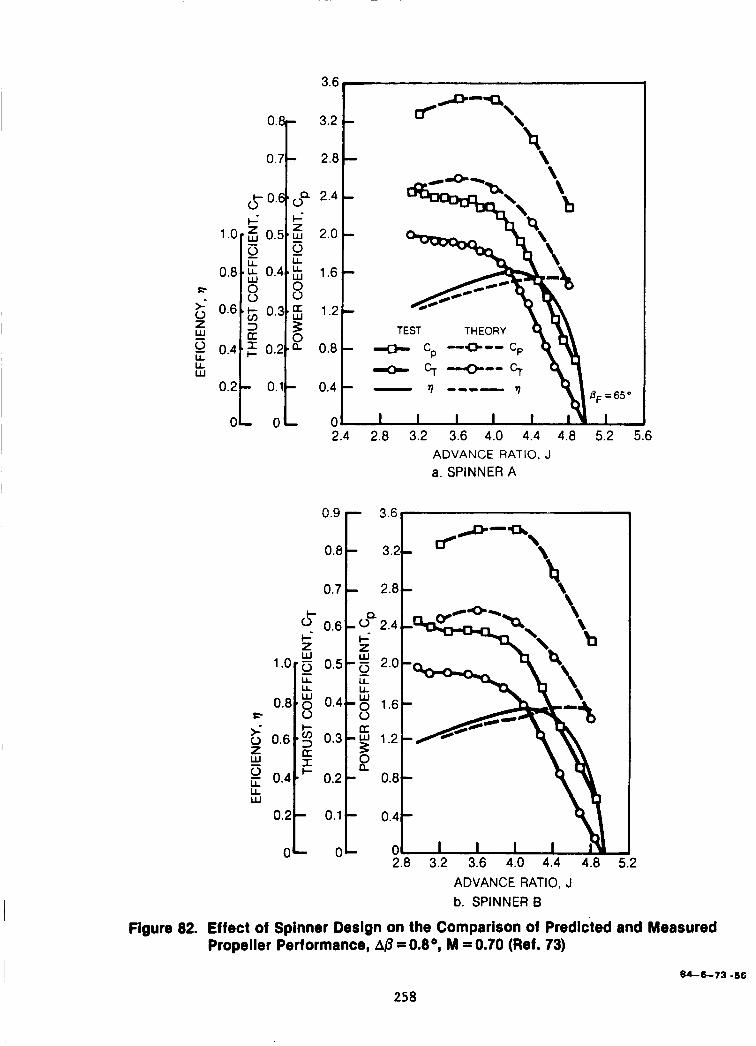
h 0.7 \

I

5.2

LL W

2.4 2.8 3.2 3.6 4.0 4.4 4.8 5.2

a. SPINNER A ADVANCE RATIO, J

5.6

0.9 0.8[ :LL 0.7 2.8

LL

LL W

0.2

2.8 3.2 3.6 4.0 4.4 4.8 ADVANCE RATIO, J b. SPINNER B

Figure 82. Effect of Spinner Design on the Comparison of Predicted and Measured Propeller Performance, A@ = 0 . 8 O , M = 0.70 (Ref. 73)

84-8-73 -68

258

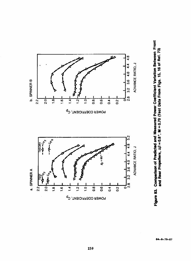
m a

z w z L v)

d

d3 'lN313133303 tl3MOd

a

ca

d3 'lN3131dd303 U3MOd

P

Y 3 z n a

P 5 w Y P n a

25 9

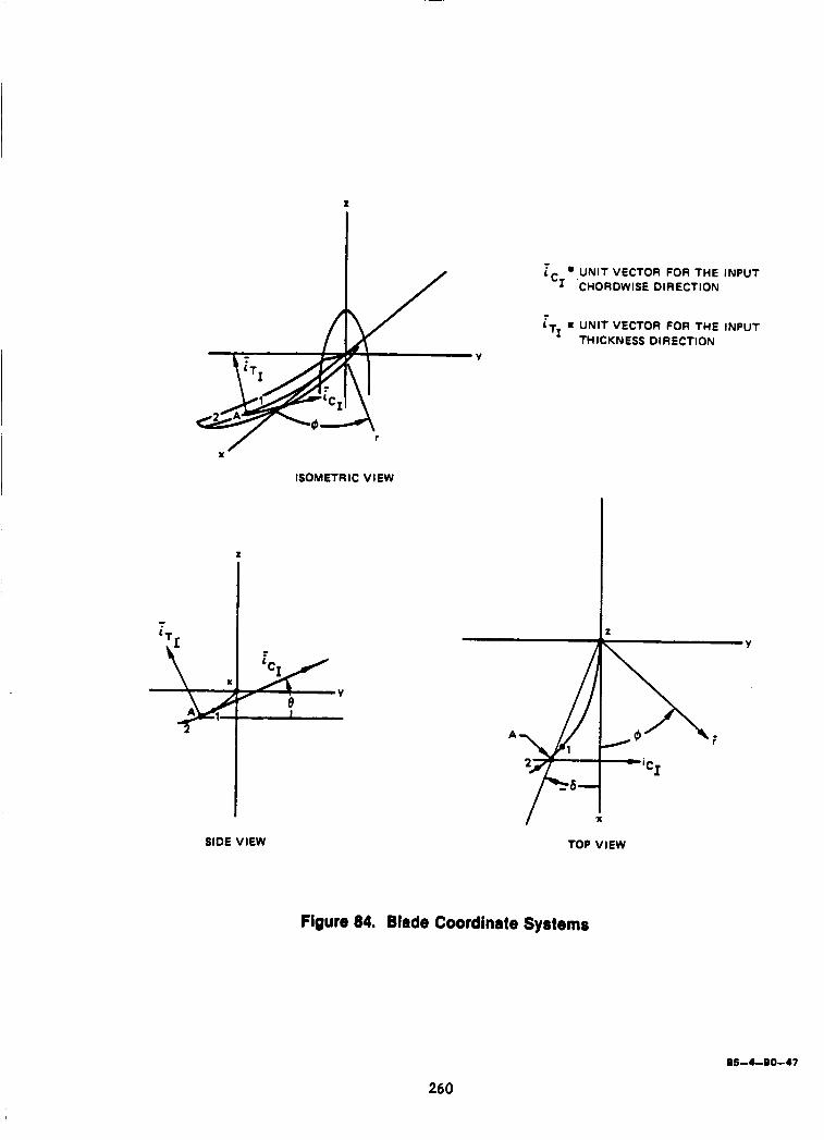
Y

X

ISOMETRIC VIEW

Y

r

X -

ISOMETRIC VIEW

SIDE VIEW

- i .,UNIT VECTOR FOR THE INPUT

CHORDWISE DIR ECTlON

- i rn UNIT VECTOR FOR THE INPUT

THICKNESS DIRECTION

I 'X

TOP VIEW

Figure 84. Blade Coordinate Systems

85-4-90-47

260

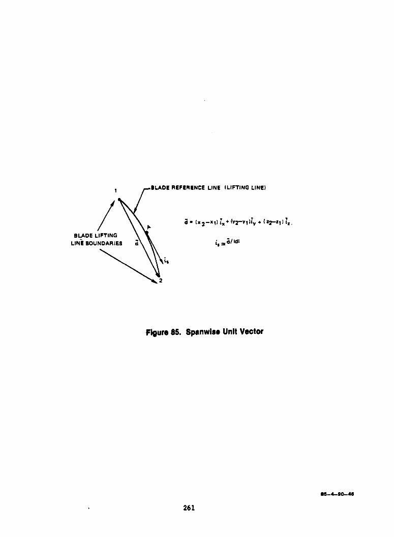
BLADE REFERENCE LINE (LIFTING LINE) 1 f

BLADE LIFTING LINE BOUNDARIES

Figure 85. Spanwise Unit Vector

85-4-00-46

26 1

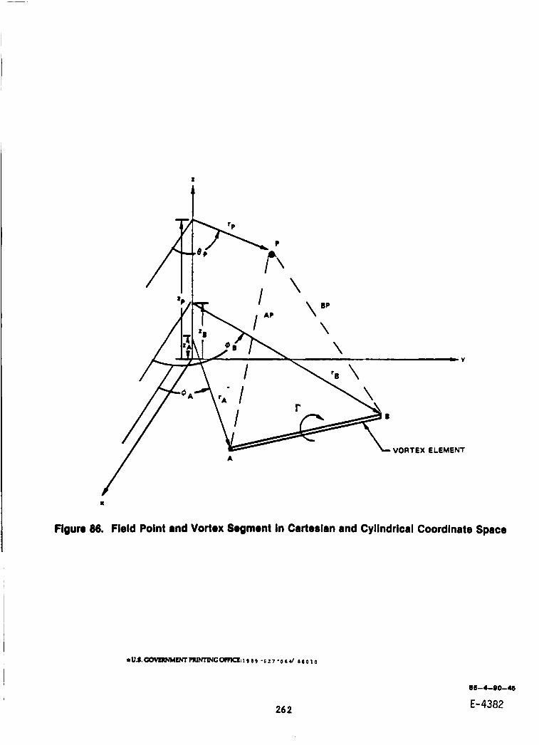
Figure 86. Fieid Point and Vortex Segment in Cartesian and Cylindrical Coordinate Space

26 2

06-4-00-46

E-4382

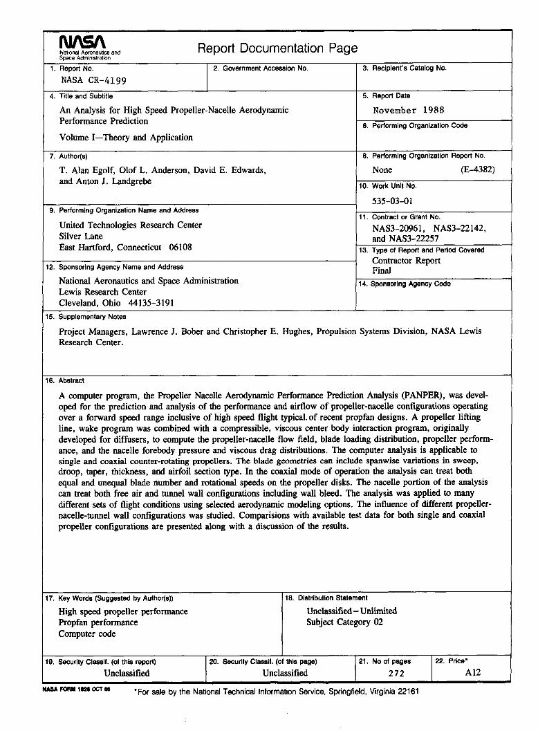
Nationd Aeronautics and

1. Report No.

NASA CR-4199

Report Documentation Page 2. Government Accession No.

4. Title and Subtitle

An Analysis for High Speed Propeller-Nacelle Aerodynamic Performance Prediction

Volume I-Theory and Application

7. Author@)

T. Alan Egolf, Olof L. Anderson, David E. Edwards, and Anton J. Landgrebe

9. Performing Organization Name and Address

United Technologies Research Center Silver Lane East Hartford, Connecticut 06 108

2. Sponsoring Agency Name and Address

National Aeronautics and Space Administration Lewis Research Center Cleveland, Ohio 44135-3191

5. Supplementary Notes

3. Recipient's Catalog No.

5. Report Date

November 1988 6. Performing Organization Code

8. Performing Organization Report No.

None (E-4382)

10. Work Unlt No.

535-03-01

11. Contract or Grant No.

and NAS3-22257

Contractor Report Final

14. Sponsoring Agency Code

NAS3-20961, NAS3-22142,

13. Type of Report and Period Covered

Project Managers, Lawrence J. Bober and Christopher E. Hughes, Propulsion Systems Division, NASA Lewis Research Center.

6. Abstract

A computer program, the Propeller Nacelle Aerodynamic Performance Prediction Analysis (PANPER), was developed for the prediction and analysis of the performance and airflow of propeller-nacelle configurations operating over a forward speed range inclusive of high speed flight typical-of recent propfan designs. A propeller lifting line, wake program was combined with a compressible, viscous center body interaction program, originally developed for diffusers, to compute the propeller-nacelle flow field, blade loading distribution, propeller performance, and the nacelle forebody pressure and viscous drag distributions. The computer analysis is applicable to single and coaxial counter-rotating propellers. The blade geometries can include spanwise variations in sweep, droop, taper, thickness, and airfoil section type. In the coaxial mode of operation the analysis can treat both equal and unequal blade number and rotational speeds on the propeller disks. The nacelle portion of the analysis can treat both free air and tunnel wall configurations including wall bleed. The analysis was applied to many different sets of flight conditions using selected aerodynamic modeling options. The influence of different propeller- nacelle-tunnel wall configurations was studied. Comparisions with available test data for both single and coaxial propeller configurations are presented along with a discussion of the results.

7. Key Words (Suggested by Author@))

High speed propeller performance Propfan performance Computer code

18. Distrlbution Statement

Unclassified - Unlimited Subject Category 02

9. Security Classif. (of this report) 20. Security Classif. (of this page) 21. No of pages 22. Price' Unclassified Unclassified 1 272 I A12

'For sale by the National Technical Information Service, Springfield, Virginia 221 61 NASA FORY 1020OClW

Documents

An Analysis for High Speed