An Algor ithm to Estimate the Two-Way Fixed EffectsModel · An Algor ithm to Estimate the Two-Way Fixed EffectsModel ... deal with situations where the panel structure is sparse,

J. Econom. Meth. 2015; aop

Practitioner ’ s Corner

Paulo Somaini * and Frank A. Wolak

An Algorithm to Estimate the Two-Way Fixed Effects Model Abstract : We present an algorithm to estimate the two-way fixed effect linear model. The algorithm relies on

the Frisch-Waugh-Lovell theorem and applies to ordinary least squares (OLS), two-stage least squares (TSLS)

and generalized method of moments (GMM) estimators. The coefficients of interest are computed using the

residuals from the projection of all variables on the two sets of fixed effects. Our algorithm has three desirable

features. First, it manages memory and computational resources efficiently which speeds up the computa-

tion of the estimates. Second, it allows the researcher to estimate multiple specifications using the same set

of fixed effects at a very low computational cost. Third, the asymptotic variance of the parameters of interest

can be consistently estimated using standard routines on the residualized data.

Keywords: Frisch-Waugh-Lovell theorem; GMM; OLS; panel data; two-way fixed effects.

DOI 10.1515/jem-2014-0008

1 Introduction Large data sets allow researchers to obtain precise estimates even after controlling for different sources of

heterogeneity. It is often the case that appropriately controlling for heterogeneity requires including two sets

of high-dimensional fixed effects. For example, consider estimating residential electricity demand using daily

consumption from a panel of 1000 households over a 5-year period. Half of the households were exposed to

real-time pricing while the other half faced a regular two-part tariff. It seems appropriate to include house-

holds fixed effects that capture heterogeneity in electricity consumption habits, and day-of-sample fixed

effects that capture common unobserved time-specific demand shocks (e.g., due to varying whether con-

ditions). If each consumer is observed 1826 times, the data would contain 1.8 million observations. Given

memory constraints, creating a set of dummies for either household or day effects is not practical and may

not be feasible at all. In this paper we propose a feasible algorithm that computes the effect of the variables

of interest (e.g., real-time prices) managing memory and computational power efficiently.

The algorithm relies on the Frisch-Waugh-Lovell theorem. The coefficients of interest are computed by

OLS, TSLS or GMM using the residuals from the projection of all variables on the two sets of fixed effects. This

procedure is trivial in balanced panels with equally-weighted observations but it can be quite complicated in

cases where observations are not equally weighted or the panel is unbalanced. The algorithm in this paper is

especially suited for the latter cases.

Let N be the number of households/groups and T be the number of periods. The data consist of approxi-

mately N × T observations. Unbalanced panels may have less observations. Panels where some households

are observed more than once in each time period may have more observations. Constructing an additional

*Corresponding author: Paulo Somaini, Department of Economics, MIT, Cambridge, MA, USA,

e-mail: [email protected]

Frank A. Wolak: Department of Economics, Stanford University, Stanford, CA, USA

Brought to you by | MIT LibrariesAuthenticated | [email protected] author's copy

Download Date | 3/13/15 2:56 AM

2 P. Somaini and F.A. Wolak: An Algorithm to Estimate the Two-Way Fixed Effects Model

set of dummies requires adding min( N , T ) – 1 variables. This is feasible only if the memory is able to store an

array with dimensions N × T × (min( N , T ) – 1). We propose an algorithm where this is not necessary. The first

step of the algorithm computes a set of three matrices that characterize the structure of fixed effects given a

particular sample. The first matrix is N by T with typical element equal to the sum of weights for observations

that share a particular pair of fixed effects. The other two matrices can be computed from the first one and

are used repeatedly in the subsequent steps. The single most computationally intensive operation in this step

is inverting a (min( N , T ) – 1) by (min( N , T ) – 1) matrix. The second step of the algorithm obtains the residuals

of the projection of each of the variables on the two sets of fixed effects. This step is computationally inex-

pensive as the matrix inversion required to compute the projection was done once and for all in the first step.

The third step is to estimate the desired specification with the residualized data using standard statistical

routines. By virtue of the Frisch-Waugh-Lovell theorem, the estimate of the asymptotic variance calculated

with the residualized data is numerically identical to the estimate calculated with the original data.

Our algorithm has three desirable features. First, it manages memory and computational resources effi-

ciently which speeds up the computation of the estimates. Second, it allows the researcher to estimate multiple

specifications using the same set of dummies at a very low computational cost. The most computational inten-

sive operation, inverting the matrix in step one, has to be performed only once no matter how many explana-

tory variables are included in the analyisis. The results of step one can be stored and used over and over as the

researcher adds more variables to the analysis and runs different specifications. Third, the asymptotic variance

of the parameters of interest can be consistently estimated using standard routines for OLS, TSLS or GMM on the

residualized data, including the estimator robust to heteroskedasticity and within-group correlation.

Standard routines available in statistical software do not deal with two-way fixed effect models efficiently.

Stata allows the user to absorb one set of fixed effects but requires generating a set of dummies for the other. In

SAS, PROC PANEL has a TWOWAY option that creates one set of dummies. Both procedures may require more

memory than available. There are some useful user-generated algorithms that avoid creating dummies. They

are specifically designed to deal with situations where the panel structure is sparse, that is, cases where N and

T are both very large but the number of observations is order of magnitudes lesser than N × T . For example,

Carneiro et al. (2012) study 12 million employment spells of N=3,000,000 employees in T=350,000 firms. Our

method inverts a T × T matrix. Stata algorithms such as reghdfe ( Guimaraes and Portugal 2010 ; Correia 2014 ),

reg2hdfe ( Guimaraes 2011 ) and a2reg ( Ouazad 2008 ) avoid matrix inversion and rely on iterative procedures

to residualize each covariate. 1 These methods will work better than ours in cases where inverting a T × T matrix

is computationally impractical and the number of covariates to residualize is small. The algorithm proposed

here is specifically designed to deal with dense panel structures where inverting a (min( N , T ) – 1) × (min( N , T ) – 1)

matrix is costly, but possible. The inverse matrix can be stored and used repeatedly when estimating different

specifications including new covariates. These covariates can be residualized at a relatively low computational

expense. Intuitively, the fixed cost of inverting the (min(N, T)–1)×(min(N, T)–1) matrix reduces the marginal cost

of residualizing additional covariates. We show that paying this fixed cost is the best alternative in many practi-

cal situations.

The rest of this paper is organized as follows. The next section describes the panel data model with

two-way fixed effects and the OLS, TSLS, and GMM estimators with their corresponding asymptotic variance.

Section 3 describes the algorithm. Section 4 compares its performance with other available methods.

2 The Panel Model Following Arellano (1987) , consider the model:

β= + + + ∈ ∈′ … … ( { 1, , }; { 1, , } ),it it i t it

y x e h u t T i N

1 Gaure (2013a) and Gaure (2013b) implement a similar iterative procedure in R.



P. Somaini and F.A. Wolak: An Algorithm to Estimate the Two-Way Fixed Effects Model 3

where y it is the outcome of household i in period t , x

it is a K × 1 vector of included variables, h

t is a time fixed

effect and e i is a group/household fixed effect. 2 The household effect e

i and the time effect h

t are unobservable

and potentially correlated with x it . There is a set of instruments z

it ( L × 1 vector, L ≥ K ) that is assumed to satisfy

the following exogeneity condition:

… … =1 1

( | , , , , , , ) 0.it i iT i T

E u z z e h h

The u it are assumed to be independently distributed across groups (or households) but no restrictions are

placed on the form of the autocovariances for a given group:

1 1

( | , , , , , , ) .i i i iT i T i

E u u z z e h h Ω… … =′ �

Each observation has a weight that can be related to the inverse of the probability of being sampled. If a

pair ( i , t ) is unobserved then w it = 0 (missing data is assumed to occur at random). Let �y denote the vector of

outcomes y it stacked by group and then ordered chronologically. Similarly, denote �X be the matrix of stacked

vectors ′it

x and �Z be the matrix of stacked vectors ′ .it

z �D is a matrix of dummies for groups and �H is a

matrix of dummies for time periods. w is the vector of weights and �u is the vector of unobserved u it . Either �H

or �D has one of its columns removed so that = + −� �([ , ]) 1.rank D H T N It is convenient to remove a column of

�H if T < N and a column of �D if N < T .

To obtain a model with constant weights, we premultiply the model by a diagonal matrix with the

squared roots of the weights arranged on the main diagonal. This transformation is equivalent to multiplying

each row in the data by the squared root of its weight. Let ( )diag w be such a matrix and = �( ) ,y diag w y

= �( ) ,u diag w u = �( ) ,X diag w X = �( ) ,Z diag w Z = �( )D diag w D and = �( ) .H diag w H The model can be

written as:

.Y X De Hh uβ= + + + (1)

Let M denote the annihilator matrix of S = [ D , H ]. M = I – S ( S ′ S ) – 1 S ′ , M = M ′ , MM = M and MS = 0. Denote y + = My ,

X + = MX , Z + = MZ . By the Frisch – Waugh – Lovell Theorem ( Frisch and Waugh 1933 ; Lovell 1963, 2008 ; Giles

1984 ), the GMM estimator of β for a weighting matrix W is:

1

1

ˆ ˆ ˆ( ) ( )

ˆ ˆ( ) ( ).

GMMX Z WZ X X Z WZ y

X Z WZ X X Z WZ u

β

β

+ + + + − + + + +

+ + + + − + + +

= ′ ′ ′ ′= + ′ ′ ′ ′

If + + −= ′ 1ˆ ( ) ,W Z Z this estimator is the TSLS estimator; if K = L , it is the instrumental variables estimator; and

if X = Z , it is the OLS estimator:

1

1

ˆ ( ) ( )

( ) ( ).

OLSX X X y

X X X u

β

β

+ + − + +

+ + − +

= ′ ′= + ′ ′

Under appropriate regularity conditions:

β β − −− → 1 1ˆ( ) ( 0, ),N N J VJ

where

− + + + +

→∞= ′ ′1 ˆplim ( )N

J N X Z WZ X

1

1

ˆ ˆplim ( ) ( ) ( ).N

N i i ii

V N X Z W Z Z WZ XΩ− + + + + + +→∞

=

⎡ ⎤= ′ ′ ′ ′⎢ ⎥

⎣ ⎦∑

2 The panel can be unbalanced. There can be unobserved pairs or pairs that are observed more than once. To keep notation sim-

ple, we will focus only on imbalances of the first kind but the algorithm handles both. This linear model has also been considered

by Davis (2002) and Wansbeek and Kapteyn (1989).




and Ω Ω= �( ) ( ).i i i i

diag w diag w Consistent estimates of the asymptotic variance can be obtained applying

standard statistical routines to the residualized data ( y + , X + , Z + ).

Consider for example the OLS estimator. Its asymptotic distribution specializes to:

1 1

1

1

1

ˆ( ) ( 0, )

plim ( )

plim ( ).

N

N

N i i ii

N N J VJ

J N X X

V N X X

β β

Ω

− −

− + +→∞

− + +→∞

=

− →= ′

= ′∑

Arellano (1987) considers three estimators of β( )OLS

avar . Let β+ + += − ˆ .i i i OLS

u y X The first estimator is robust to

heteroskedasticity and within-group correlation:

1 1

11

ˆ( ) ( ) ( ) .N

OLS i i i ii

avar X X X u u X X Xβ + + − + + + + + + −

=

⎛ ⎞= ′ ′ ′ ′⎜ ⎟⎝ ⎠∑

(2)

This estimator can be calculated clustering standard errors at the group level. 3 The second estimator will

produce consistent standard errors if x it and u

it have finite 12th moments ( Stock and Watson 2008 , Remark 7)

and disturbances are homoskedastic, i.e., Ω i = Ω for all i :

1 1

21

ˆ ˆ( ) ( ) ( ) ,N

OLS i ii

avar X X X X X Xβ Ω+ + − + + + + + −

=

⎛ ⎞= ′ ′ ′⎜ ⎟⎝ ⎠∑

(3)

where

1

1

ˆ .N

i ii

N u uΩ+ − + +

=

= ′∑

(4)

The third estimator will produce consistent standard errors under the classical assumption Ω i = σ 2 I :

2 1

3ˆ ˆ( ) ( ) ,

OLSavar X Xβ σ + + −′= (5)

where

2ˆu u

L N T Kσ

+ +′=− − −

and L is the number of observations. This estimator can be calculated running the regression of y + on X + and

multiplying the estimate of the asymptotic variance of βOLS

by −

− − −.

L K

L N T K

3 The Algorithm In balanced panels with constants weights in one of the two dimensions – w

it = w

i or w

it = w

t – the computation

of β and its asymptotic variance is straightforward. y + is obtained subtracting the weighted mean of �y along

both dimensions:

+ = − −�it it i t

y y y y

3 In Stata: reg plus_y plus_x*, vce(cluster h)




where

( )−= =∑∑

∑ ∑��

and .it it iit it it

i t

it itt i

w y yw yy y

w w

X + and Z + are computed following the same procedure. This heuristic approach can be justified formally.

Premultiplying the original model in equation (1) first by M D , the annihilator of D , and then by M

H , the

annihilator of H , results in:

.H D H D H D

M M Y M M X M M Hh uβ= + + (6)

If the panel is balanced and weights are constant in t or in i , then M H M

D = M

H or M

H M

D = 0. In either case,

M H M

D H = 0, and the transformed model does not depend on the fixed effects.

If the panel is unbalanced or the group weights vary, 0 ≠ M H M

D ≠ M

H and the transformation M

H M

D does

not eliminate the fixed effects in matrix H . The fixed effects are annihilated only if the model is premultiplied

by M = I – S ( S ′ S ) – 1 S ′ where S = [ D , H ]. The algorithm presented in this paper is specifically designed to deal with

these cases and consists of three steps:

1. Compute ( S ′ S ) – 1 . This step requires inverting a (min( N , T ) – 1) by (min( N , T ) – 1) matrix and storing it along

with two N-by-T matrices. These three matrix contain all the information required to construct the anni-

hilator matrix M .

2. Obtain ( y + , X + , Z + ).

3. Use standard methods to estimate β and its asymptotic variance by OLS, TSLS or GMM.

Only the first step is computationally intensive as it requires inverting a potentially large matrix. This step

only has to be performed once for a given panel structure. The compuational cost of residualizing variables

and running different specifications with them is relatively low.

3.1 Computation of ( S ′ S ) – 1

According the the definition of S ,

1

1( ) .D D D H

S SD H H H

−

−⎡ ⎤′ ′

=′ ⎢ ⎥′ ′⎢ ⎥⎣ ⎦

D ′ D is a diagonal matrix with typical diagonal element ( i , i ) equal to Σ t w

it . Similarly, H ′ H is a diagonal matrix

with typical diagonal element ( t , t ) equal to Σ i w

it . D ′ H is a N -by- T matrix with typical element ( i , t ) equal to w

it .

Using the formula for the inverse of a partitioned matrix:

−⎡ ⎤ ⎡ ⎤′ ′

=⎢ ⎥ ⎢ ⎥′ ′ ′⎢ ⎥ ⎢ ⎥⎣ ⎦ ⎣ ⎦

1

,A B D D D H

B C D H H H

(7)

( ) 11( ) ( )A D D D H H H H D

−−= −′ ′ ′ ′ (8)

( ) 11( ) ( )C H H H D D D D H

−−= −′ ′ ′ ′ (9)

1 1( ) ( ) .B AD H H H D D D HC− −=− =−′ ′ ′ ′ (10)

If T < N , the first step of the algorithm calculates and stores C , B , D ′ H and ( D ′ D ) – 1 ( C is T – 1 by T – 1, D ′ H and

B are N by T – 1 and D ′ D is N by N but it is diagonal, so N numbers are stored). The only non-diagonal matrix

that is inverted is (9). A can be calculated from the stored matrices by




− − −= +′ ′ ′ ′ ′1 1 1( ) ( ) ( ) .A D D D D D HCH D D D (11)

To economize computing power and memory, A – an N by N matrix – is not constructed.

If N < T , this step calculates and stores A , B , D ′ H and ( H ′ H ) – 1 ( A is N – 1 by N – 1, D ′ H and B are N – 1 by T and

H ′ H is T by T but it is diagonal, so T numbers are stored). The only non-diagonal matrix that is inverted is (8).

C can be calculated by

− − −= +′ ′ ′ ′ ′1 1 1( ) ( ) ( ) .C H H H H H DAD H H H (12)

However, C is never constructed or stored.

Notice that the algorithm never constructs or stores a non-diagonal square matrix of size equal to the

greatest of T and N . This feature of the algorithm makes it more robust to memory constraints.

3.2 The residualized data ( y + , X + , Z + )

We obtain the projection coefficients

δ

τ

= +′ ′= +′ ′ ′

ˆ

ˆ

AD y BT y

B D y CT y

and compute δ τ+ = − −ˆ ˆ.y y D T Variables +k

x in X + , and +k

z in Z + are obtained in the same way.

If T < N , the matrix A is replaced by the expression in (11). D ′ y is a N -th order vector so AD ′ y can be

calculated without ever creating A or any other N by N matrix that is not diagonal:

1 1 1( ) ( ) ( ) ( ) ( )( ) ( ).AD y D D D y D D D H C H D D D D y− − −= −′ ′ ′ ′ ′ ′ ′ ′

Similarly, If T > N , CT ′ y is calculated without ever creating C or any other T by T matrix that is not diagonal.

3.3 Estimation of the parameters and their asymptotic variance

The residualized data ( y + , X + , Z + ) can be used as if it was the original data in any statistical package. In Stata,

for example, reg plus_y plus_x*, vce(cluster h) returns βOLS

along with its asymptotic variance

estimate that is robust to within group correlation; ivregress gmm plus_y (plus_x* = plus_z*),

wmatrix(cluster h) returns βGMM

where the weighting matrix W is set equal to

1

1

1

.N

i i i ii

N Z u u Z

−

− + + + +

=

⎛ ⎞′ ′⎜ ⎟⎝ ⎠∑

Stata also returns a consistent estimate of the asymptotic variance of β .GMM

ivregress 2sls plus_y

(plus_x = plus_z), vce(robust) returns a two-stage least square estimate of β along with a hetero-

skedasticity robust estimate of its asymptotic variance. If vce(robust) is omitted, the asymptotic variance

is estimated by (5), which is consistent under the classical assumption that the error terms are independently

and identically distributed ( Ω i = σ 2 I ). The reported variance estimates can be multiplied by

L K

L N T K

−− − − to

account for the reduced degrees of freedom.4

4 See textbooks such as Hayashi (2000) and Wooldridge (2010) for further discussion on different estimators of the asymptotic

variance. Baum (2007) discusses their implementation in Stata.




4 Comparative Performance Analysis This section compares the performance of the proposed algorithm with four existing algorithms in Stata:

reghdfe , reg2hdfe , a2reg and felsdvreg . The comparisons are not totally fair as these algorithms

have been designed to work in sparse panel models that are typical in labor studies (Abowd et al. 1999;

Carneiro et al. 2012). They are still the best available options even for dense panels.

We implemented the algorithm in mata , the matrix language in Stata. We wrote a Stata program called

res2fe which follows Stata conventions and calls the mata routines. res2fe stands for “ Residualize two

fixed effects. ” For example, if hhid is a variable that contains a household identifier and tid contains an

hour-of-sample identified, then res2fe, abs(hhid tid) root("C:/abc") performs the first step of

the algorithm for a pair of fixed effects and stores the required matrices in the file C:/abc. If consumption

and hourprice are the endogenous and exogenous variables, respectively, reg2fe consumption hour-

price, root("C:/abc"), p(plus_) creates the variables plus_consumption plus_hourprice

that contain the residualized version of the original variables. reg2fe consumption hourprice,

abs(hhid tid) root("C:/abc"), p(plus_) preforms both steps. 5 The actual estimation is per-

formed using the built-in commands regress or ivregress on the residualized variables.

The command a2reg , proposed by Ouazad (2008), uses a Conjugate gradient method to solve the

minimum squares problem and obtain β .OLS

The algorithm never computes X ′ X ; therefore, it does not report

an estimate of the asymptotic variance. The commands reghdfe ( Correia 2014 ) and reg2hdfe ( Guimaraes

2011 ) follow iterative procedures proposed by Guimaraes and Portugal (2010) to obtain the solution without

the explicit calculation of any inverse matrix. They residualize the dependent and independent variables by

sequentially projecting them on the two sets of dummies. While computationally intensive, this approach

imposes minimum memory requirements. Another advantage of these algorithms is that they also rely

on the FWL theorem and generate residualized variables that can be stored for future use. The command

felsdvreg, proposed by Cornelissen (2008) , absorbs one set of fixed effects and constructs components of

the OLS normal equations using the identifier of the other set of fixed effects. Thus, it solves for βOLS

without

creating a set of dummies or relying on an iterative process.

We generate a panel of N = 10 n households and T = 10 t time periods and randomly drop 10 percent of the

observations. The resulting panel is unbalanced. We draw household-specific and time-specific fixed effect

from a standard normal. We also draw K covariates x and errors υ from independent standard normals. The

dependent variable y is:

υ=

= + + +∑1

K

it itk i t itk

y x d h

We estimate the parameters of the model using our procedure ( res2fe ) and the four existing algorithms and

compare their running time over 10 different runs. Notice that the panel structure is different in each draw,

so we are not taking advantage of the fact that our method allows to run the matrix inversion in step one just

once. We stopped at 10 draws per configuration because the variance of the running times was very low rela-

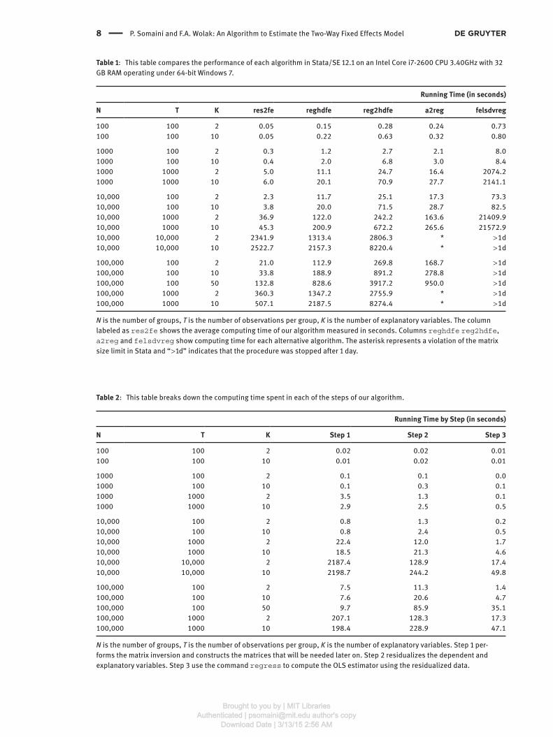
tive to the differences in means across configurations. Table 1 summarizes the results for different values of

N , T and K .

Table 1 shows that our procedure outperforms algorithms designed for sparse panels. The only exception

is the case with N = T = 10,000 when res2fe spends too much time inverting a 9999 × 9999 matrix. reghdfe

performs the estimation much faster. Even this case is useful to illustrate one of the advantages of our proce-

dure. The increase in computing time from K = 2 to K = 10 is relatively small compared to the increase observed

5 See the documentation to the Stata code for additional details. The algorithm was also implemented in Matlab and SAS to take

advantage of some specific features of those programs. The Matlab implementation uses sparse matrices and takes advantage of a

faster algorithm to invert matrices. The SAS implementation never loads the raw data in the computer RAM memory.




Table 1 : This table compares the performance of each algorithm in Stata/SE 12.1 on an Intel Core i7-2600 CPU 3.40GHz with 32

GB RAM operating under 64-bit Windows 7.

Running Time (in seconds)

N T K res2fe reghdfe reg2hdfe a2reg felsdvreg

100 100 2 0.05 0.15 0.28 0.24 0.73

100 100 10 0.05 0.22 0.63 0.32 0.80

1000 100 2 0.3 1.2 2.7 2.1 8.0

1000 100 10 0.4 2.0 6.8 3.0 8.4

1000 1000 2 5.0 11.1 24.7 16.4 2074.2

1000 1000 10 6.0 20.1 70.9 27.7 2141.1

10,000 100 2 2.3 11.7 25.1 17.3 73.3

10,000 100 10 3.8 20.0 71.5 28.7 82.5

10,000 1000 2 36.9 122.0 242.2 163.6 21409.9

10,000 1000 10 45.3 200.9 672.2 265.6 21572.9

10,000 10,000 2 2341.9 1313.4 2806.3 * > 1d

10,000 10,000 10 2522.7 2157.3 8220.4 * > 1d

100,000 100 2 21.0 112.9 269.8 168.7 > 1d

100,000 100 10 33.8 188.9 891.2 278.8 > 1d

100,000 100 50 132.8 828.6 3917.2 950.0 > 1d

100,000 1000 2 360.3 1347.2 2755.9 * > 1d

100,000 1000 10 507.1 2187.5 8274.4 * > 1d

N is the number of groups, T is the number of observations per group, K is the number of explanatory variables. The column

labeled as res2fe shows the average computing time of our algorithm measured in seconds. Columns reghdfe reg2hdfe ,

a2reg and felsdvreg show computing time for each alternative algorithm. The asterisk represents a violation of the matrix

size limit in Stata and “ > 1d ” indicates that the procedure was stopped after 1 day.

Table 2 : This table breaks down the computing time spent in each of the steps of our algorithm.

Running Time by Step (in seconds)

N T K Step 1 Step 2 Step 3

100 100 2 0.02 0.02 0.01

100 100 10 0.01 0.02 0.01

1000 100 2 0.1 0.1 0.0

1000 100 10 0.1 0.3 0.1

1000 1000 2 3.5 1.3 0.1

1000 1000 10 2.9 2.5 0.5

10,000 100 2 0.8 1.3 0.2

10,000 100 10 0.8 2.4 0.5

10,000 1000 2 22.4 12.0 1.7

10,000 1000 10 18.5 21.3 4.6

10,000 10,000 2 2187.4 128.9 17.4

10,000 10,000 10 2198.7 244.2 49.8

100,000 100 2 7.5 11.3 1.4

100,000 100 10 7.6 20.6 4.7

100,000 100 50 9.7 85.9 35.1

100,000 1000 2 207.1 128.3 17.3

100,000 1000 10 198.4 228.9 47.1

N is the number of groups, T is the number of observations per group, K is the number of explanatory variables. Step 1 per-

forms the matrix inversion and constructs the matrices that will be needed later on. Step 2 residualizes the dependent and

explanatory variables. Step 3 use the command regress to compute the OLS estimator using the residualized data.




for reghdfe . This is true also in the other cases where res2fe ourperforms reghdfe . Our method only

requires inverting the matrix once independently of the number of explanatory variables K . The maximum

relative efficiency gain of our method relative to reghdfe occurs when T is low and K is high. In particular,

if N = 100,000, T = 100 and K = 50, res2fe running time was a sixth of that of reghdfe .

Table 2 shows that the computing time employed in step 1, which performs the inversion, does not

depend on K . The computing time in step 2, which projects each explanatory variables on the set of fixed

effects, is increasing in K .

The comparative performance analysis suggests that res2fe works best for dense panels where one

fixed effect dimension is large and the other is large enough so that creating additional dummy variables is

impractical, but small enough so that inverting a matrix of that dimension is computationally trivial. When

inverting such a matrix is impractical, iterative procedures such as reghdfe perform better.

5 Final Remarks We present an algorithm to estimate a two-way fixed effect linear model. While existent algorithms are

designed for sparse panels, ours works best in dense, but unbalanced panels. The algorithm relies on the

Frisch-Waugh-Lovell Theorem and applies to ordinary least squares, two-stage least squares and general-

ized method of moments estimators. The coefficients of interest are computed using the residuals from the

projection of all variables on the two sets of fixed effects. Our algorithm has three desirable features. First, it

manages memory and computational resources efficiently which speeds up the computation of the estimates.

Second, it allows the researcher to estimate multiple specifications using the same set of fixed effects at a

very low computational cost. Third, the asymptotic variance of the parameters of interest can be consistently

estimated using standard routines on the residualized data. This algorithm is preferable to existent ones

when the panel is dense, one fixed effect dimension is large and the other is large enough so that creating

additional dummy variables is impractical, but small enough so that inverting a matrix of that dimension is

computationally feasible.

References Abowd, J. M., F. Kramarz, and D. N. Margolis (1999): “High Wage Workers and High Wage Firms,” Econometrica 67 (2): 251–333.

Arellano, M. 1987. “ Computing Robust Standard Errors for Within-Groups Estimators. ” Oxford Bulletin of Economics and Statistics 49 (4): 431 – 434.

Baum, C. F., M. E. Schaffer, and S. Stillman. 2007. “ Enhanced Routines for Instrumental Variables/GMM Estimation and

Testing. ” Stata Journal 7 (4): 465 – 506.

Carneiro, A., P. Guimares, and P. Portugal (2012): “Real Wages and the Business Cycle: Accounting for Worker, Firm, and Job Title

Heterogeneity,” American Economic Journal: Macroeconomics 4(2): 133–152.

Cornelissen, T. 2008. “ The Stata Command Felsdvreg to Fit a Linear Model with Two High-Dimensional Fixed Effects. ” Stata Journal 8 (2): 170 – 189.

Correia, S. 2014. “REGHDFE: Stata Module to Perform Linear or Instrumental-Variable Regression Absorbing Any Number of

High-Dimensional Fixed Effects,” Statistical Software Components S457874, Boston College Department of Economics.

Davis, P. 2002. “ Estimating Multi-Way Error Components Models with Unbalanced Data Structures. ” Journal of Econometrics 106

(1): 67 – 95.

Frisch, R., and F. V. Waugh. 1933. “ Partial Time Regressions as Compared with Individual Trends. ” Econometrica 1 (4): 387 – 401.

Gaure, S. 2013a. “ Lfe: Fitting Linear Models with Multiple Factors with Many Levels. ” The R Journal 5(2): 104–116.

Gaure, S. 2013b. “ OLS with Multiple High Dimensional Category Variables. ” Computational Statistics & Data Analysis 66: 8 – 18.

Giles, D. E. A. 1984. “ Instrumental Variables Regressions Involving Seasonal Data. ” Economics Letters 14 (4): 339 – 343.

Guimaraes, P. 2009. “REG2HDFE: Stata Module to Estimate a Linear Regression Model with two High Dimensional Fixed Effects,”

Statistical Software Components S457101, Boston College Department of Economics.

Guimaraes, P., and P. Portugal. 2010. “ A Simple Feasible Procedure to Fit Models with High-Dimensional Fixed Effects. ” Stata Journal 10 (4): 628 – 649.

Hayashi, F. 2000. Econometrics . Princeton: Princeton University Press.




Lovell, M. C. 1963. “ Seasonal Adjustment of Economic Time Series and Multiple Regression Analysis. ” Journal of the American Statistical Association 58 (304): 993 – 1010.

Lovell, M. C. 2008. “ A Simple Proof of the FWL Theorem. ” The Journal of Economic Education 39 (1): 88 – 91.

Ouazad, A. 2008. “A2REG: Stata Module to Estimate Models with Two Fixed Effects,” Statistical Software Components S456942,

Boston College, Department of Economics.

Stock, J. H., and M. W. Watson. 2008. “ Heteroskedasticity-Robust Standard Errors for Fixed Effects Panel Data Regression. ”

Econometrica 76 (1): 155 – 174.

Wansbeek, T., and A. Kapteyn. 1989. “ Estimation of the Error-Components Model with Incomplete Panels. ” Journal of Econometrics 41 (3): 341 – 361.

Wooldridge, J. M. 2010. Econometric Analysis of Cross Section and Panel Data . 2nd ed. Cambridge, Mass: The MIT Press.

Supplemental Material : The online version of this article (DOI: 10.1515/jem-2014-0008) offers supplementary material,

available to authorized users.



Documents

An Algor ithm to Estimate the Two-Way Fixed EffectsModel · An Algor ithm to Estimate the Two-Way Fixed EffectsModel ... deal with situations where the panel structure is sparse,