Amulti-dimensionalmonotonicniteelementmodelfor ...homepage.ntu.edu.tw/~twhsheu/member/paper/78-2002.pdfxx+R f=Ru x+ 4 −) 3 +u2 − h2R 6 xx+H:O:T: (12) isderivedsubjecttotheconsistencyrequirement

INTERNATIONAL JOURNAL FOR NUMERICAL METHODS IN FLUIDSInt. J. Numer. Meth. Fluids 2002; 39:639–656 (DOI: 10.1002/�d.351)

A multi-dimensional monotonic �nite element model forsolving the convection–di�usion-reaction equation

Tony W. H. Sheu∗;† and Harry Y. H. Chen

Department of Engineering Science and Ocean Engineering; National Taiwan University; 73 Chou-Shan Rd.;Taipei; Taiwan; Republic of China

SUMMARY

In this paper, we develop a �nite element model for solving the convection–di�usion-reaction equationin two dimensions with an aim to enhance the scheme stability without compromising consistency.Reducing errors of false di�usion type is achieved by adding an arti�cial term to get rid of threeleading mixed derivative terms in the Petrov–Galerkin formulation. The �nite element model of thePetrov–Galerkin type, while maintaining convective stability, is modi�ed to suppress oscillations aboutthe sharp layer by employing the M -matrix theory. To validate this monotonic model, we consider testproblems which are amenable to analytic solutions. Good agreement is obtained with both one- andtwo-dimensional problems, thus validating the method. Other problems suitable for benchmarking theproposed model are also investigated. Copyright ? 2002 John Wiley & Sons, Ltd.

KEY WORDS: convection–di�usion-reaction equation; two dimensions; Petrov–Galerkin formulation;M -matrix theory; monotonic

1. INTRODUCTION

The scalar convection–di�usion-reaction (CDR) equation is examined as a linear model forsimulating time-dependent equations in areas of �uid dynamics and heat transfer. In addi-tion, this equation is practically important, as it is akin to the constitutive equations used tomodel the transport of turbulent kinetic energy and its dissipation [1]. In addition, constitu-tive equations for the extra stress tensor in viscoelastic �uid �ows fall into this category [2].In an externally applied magnetic �eld, the magnetic induction equation for liquid metals isclassi�ed as the CDR equation as well [3]. The Helmholtz equation, a special form of CDRequation, governs wave propagation in areas of exterior and �bre acoustics [4]. It is this wideapplication scope that makes numerical investigation of CDR equation worthwhile.

∗ Correspondence to: Tony W. H. Sheu, Department of Engineering Science & Ocean Engineering, NationalTaiwan University, 73 Chou-Shan Road; Taipei, Taiwan, Republic of China.

† E-mail: [email protected]

Contract=sponsor: National Science Council; contract=grant number: NSC88-2611-E-002-025.

Received August 2001Copyright ? 2002 John Wiley & Sons, Ltd. Revised October 2001

640 TONY W. H. SHEU AND HARRY Y. H. CHEN

Compared with the considerable amount of e�ort that has been invested in developing theconvection–di�usion schemes, fewer studies have been devoted to the more general CDRequation [5–11] and the development of discontinuity-capturing CDR schemes [12–14]. Areliable CDR model must have the ability to render accurate solutions while suppressingnumerical oscillations of di�erent kinds. The problem of numerical instability stems from theoccurrence of convection and reaction terms. It is, therefore, necessary to construct stabilizationschemes, and this motivated the present study. In this paper, we are also concerned withprediction accuracy since we do not regard a scheme as useful if it cannot provide accuracyto a certain high level in the computation of two-dimensional problems. Another goal in thepresent model development is to resolve �eld variables in the vicinity of sharp layers.The rest of this paper is organized as follows. Section 2 presents the working equation.

This is followed by presentation of the one-dimensional �nite element model. The essentialelements of the proposed model are then presented in greater detail in Section 4. Our emphasisis on obtaining results that are less contaminated by false di�usion errors and on obtainingoscillation-free solutions in the vicinity of sharp layers. Section 5 presents numerical resultsthat can demonstrate the validity of the method. In Section 6, we give concluding remarks.

2. WORKING EQUATIONS

The following CDR equation is often considered as the model equation for schemes developedto solve the �uid dynamics and heat transfer problems:

�t + �u�x + �v�y − ��(�xx + �yy) + �R�=0 (1)

In the above, �u and �v represent the velocity components along the x and y directions, respec-tively. Other coe�cients involve �� and �R, which denote the di�usion (or �uid viscosity) andthe reaction coe�cient, respectively. By conducting the Euler implicit time-stepping schemeon �t , we can obtain the steady-state CDR equation u�x + v�y − �(�xx + �yy) + R�=f,where u= �u�t; v= �v�t; R=(1+ �R�t) and f=�n. It is, therefore, instructive to analyse thefollowing model equation:

u�x + v�y − �(�xx + �yy) + R�=f (2)

We shall, for illustrative purposes, assume that (u; v); �, and R are constant throughout. Forsimplicity, the value of � is sought subject to �= g on the boundary @�.

3. FINITE ELEMENT MODEL

Like other numerical methods, the �nite element method has a sound mathematical basis forproving the convergence of solutions. Apart from this theoretical foundation, the �nite elementmethod is favourably used when solving problems involving complex geometry. Within theweighted residual framework, the �nite element solution for Equation (2) is computed using∫Wi(u · ∇� − �∇2� + R�) d�=

∫Wif d�. The key to obtaining highly accurate solutions

exhibiting the non-oscillatory property lies in choosing an appropriate weighting function Wi.We shall, in what follows, address the construction of Wi in the linear element context.

Copyright ? 2002 John Wiley & Sons, Ltd. Int. J. Numer. Meth. Fluids 2002; 39:639–656

CONVECTION–DIFFUSION-REACTION EQUATION 641

To simplify matters in the case of high Peclet, we will �rst derive Wi based on the followingone-dimensional CDR equation:

u∇�− �∇2�+ R�=f (3)

The Galerkin representation of Equation (3) in a linear element �e = {xi; xi+1} takes thefollowing matrix form:

−uh2

uh2

−uh2

uh2

�i

�i+1

+

�h2

−�h2

−�h2

�h2

�i

�i+1

+

R3

R6

R6

R3

�i

�i+1

=

13

16

16

13

fi

fi+1

(4)

In the above, h(≡ xi+1− xi) denotes the grid size. The assemblage of two elements having thenodal point i in common results in the �nite element equation for �i

(−u2h

− �h2+R6

)�i−1 +

(2�h2+2R3

)�i +

(u2h

− �h2+R6

)�i+1

=16fi−1 +

23fi +

16fi+1 (5)

Equation (5) shows that the dominance of the matrix diagonal decreases as the reactioncoe�cient decreases and the velocity |u| increases. As the accompanying instabilities arenumerical in origin, re�nement of Wi from the shape function Ni is warranted. In keepingwith the above, Wi (i=1; 2) is expressed as follows:

Wi=Ni + �u@Ni@x

+ Pi (6)

The last two terms are introduced for stabilizing the scheme applied in the case of high Pecletnumber R1

R1 =uh�

(7)

and low reaction number R2

R2 =Rh2

�(8)

Substituting (6) into Equation (2), the linear �nite element equation at an arbitrary point iis derived from ∫

�

(Ni + �u

@Ni@x

+ Pi

)(u∇�− �∇2�+ R�− f) d�=0 (9)



As our goal is to enhance Galerkin formulation, we need to re�ne the third matrix inEquation (4) by introducing parameters � and �. One can change

R3

1

12

12

1

to

R3

[� ��

]

by choosing P1 and P2 as

P1 = 16(−3 + 2�+ �) + 1

2(1− 2�+ �)� (10)

P2 = 16(−3 + 2�+ �)− 1

2 (1− 2�+ �)� (11)

where −16�61 denotes the master co-ordinate. After some algebra, the following modi�edequation [15] for (9):

u�x − �uxx + R�− f=Ru��x +[�4(�− �)3

+ u2�− �h2R6

]�xx +H:O:T: (12)

is derived subject to the consistency requirement

�+ 2�=3 (13)

The weighting functions Pi (i=1; 2) are thus obtained as

P1 =−(1− �)� (14)

P2 = (1− �)� (15)

The resulting discrete equation is derived as follows in a domain with a uniform grid size:

{[sgn(m)

(R1 − u�

hR2

)− 6 + 4�+ �

3R2 − 2u�

hR1

]�i+m

}m={−1;1}

+[12− 8�+ 2(3− �)

3R2 +

4u�hR1

]�i

={[sgn(m)

( u�hRR2

)+�3RR2

]fi+m

}m={−1;1}

+[2(3− �)3R

R2

]fi=0 (16)

To present the discrete equation in a somewhat more compact form, the sign notation sgn(◦)shown above is employed.



−1000500

0

500

1000

u20000

40000

60000

80000

100000

R

00.00010.00020.00030.00040.0005

τ

−

u

Figure 1. The plot of � in the domain −1000¡u¡1000; 10¡R¡100 000.

To complete the �nite element model development, we need to determine � shown in(6) and � shown in (14) and (15). Our aim in determining them is to optimize the �niteelement model. To this end, the analytic solution, �exact =C1 exp(u=2�+(1=2�)

√u2 + 4R�)+

C2 exp(u=2�− (1=2�)√u2 + 4R�), is substituted into the discrete equation (5), we can derive

� and � as follows after some algebra:

�=hu

[R1R2+

sinh(R1)cosh(R1)− cosh( 12

√R21 + R2)

](17)

�=3R2

{2(R21 + 3R2)(R2 + 12)

+[R2 cosh(R1) + 2R1 sinh(R1)]

(R2 + 12)[cosh(R1)− cosh( 12√R21 + R2)]

}(18)

In the above, C1 and C2 are two arbitrary constants. For clarity, we plot � and � in Figures 1and 2 in terms of u and R, respectively. In the limiting case of zero reaction, � in Equation (17)turns out to be that proposed by Hughes and Brooks [16]. It is also interesting to �nd thatlimR→0 �=1. This is desirable since 06�61 over the entire range of R.Before proceeding with the next section, it is worth noting that use of � and � from Equa-

tions (17) and (18) renders a nodally exact solution to the model equation (3). Speci�cation ofthese analytic convection and reaction coe�cients forms the building block for the subsequenttwo-dimensional �nite element model development.

4. TWO-DIMENSIONAL FINITE ELEMENT MODEL

The goal in developing the CDR �nite element model in two dimensions is to retain thedesirable feature of its one-dimensional model. For this reason, we exploit the tensor product



−1000

−500

0

500

1000

u20000

40000

60000

80000

100000

R

00.250.5

0.75

1

λ

u

Figure 2. The plot of � in the domain −1000¡u¡1000; 10¡R¡100 000.

1

4 3

2

Figure 3. Numbering strategy for the bi-linear element.

operator

Wi=Ni + �xu@Ni@x

+ �yv@Ni@y

+ Pi (19)

In the above, Ni (i=1∼ 4) represents the bilinear shape functions. As a good stabilizationmeans for the positive-valued reaction term, we introduce six coe�cients �x; �y; �x; �y; �x, and�y when constructing Pi. Referring to the element numbering schematic shown in Figure 3,P1∼P4 are expressed as

P1 = P(−1;−1) (20a)

P2 = P(1;−1) (20b)

P3 = P(1; 1) (20c)

P4 = P(−1; 1) (20d)



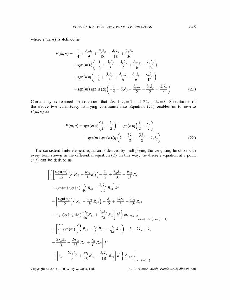
where P(m; n) is de�ned as

P(m; n) =−14+�x�y9+�y�x18

+�x�y18

+�x�y36

+ sgn(m)�(−14+�x�y3

− �y�x6+�x�y6

− �x�y12

)

+sgn(n)�(−14+�x�y3+�y�x6

− �x�y6

− �x�y12

)

+sgn(m) sgn(n)��(−14+ �x�y − �y�x

2− �x�y

2+�x�y4

)(21)

Consistency is retained on condition that 2�x + �x=3 and 2�y + �y=3. Substitution ofthe above two consistency-satisfying constraints into Equation (21) enables us to rewriteP(m; n) as

P(m; n) = sgn(m)�(12− �x2

)+ sgn(n)�

(12− �y2

)

+sgn(m) sgn(n)��(2− 3�x

2− 3�y

2+ �x�y

)(22)

The consistent �nite element equation is derived by multiplying the weighting function withevery term shown in the di�erential equation (2). In this way, the discrete equation at a point(i; j) can be derived as

[{[sgn(m)12

(�yRx1 − u�x

hRx2

)− �y2+�x�y3

− u�x6hRx1

− sgn(m) sgn(n) v�y4kRx1 +

�x�y72

Rx2

]k2

+[sgn(n)12

(�xRy1 − v�y

kRy2

)− �x2+�x�y3

− v�y6kRy1

− sgn(m) sgn(n) u�x4hRy1 +

�x�y72

Ry2

]h2}�i+m; j+n

]m={−1;1}; n={−1;1}

+[{[

sgn(m)(12Rx1 − �y

6Rx1 − u�x

3hRx2

)− 3 + 2�x + �y

− 2�x�y3

− 2u�x3h

Rx1 +�x6Rx2

]k2

+[�x − 2�x�y

3+v�y3kRy1 − �x�y

18Ry2

]h2}�i+m; j

]m={−1;1}



+[{[

sgn(n)(12Ry1 − Ry1 �x6 − v�y

3kRy2

)− 3 + 2�y + �x

− 2�x�y3

− 2v�y3k

Ry1 +�y6Ry2

]h2

+[�y − 2�x�y

3+u�x3hRx1 − �x�y

18Rx2

]k2}�i; j+n

]n={−1;1}

+[(12Rx2 − �x

6Rx2 − �y

6Rx2 +

�x�y18Rx2 +

4u�x3h

Rx1

+ 6− 4�x − 2�y + 4�x�y3)k2

+(12Ry2 − �x

6Ry2 − �y

6Ry2 +

�x�y18

Ry2 +4v�y3kRy1

+ 6− 4�x − 2�y + 4�x�y3)h2]�i; j

={112

[(−sgn(m)u�xh

Rx2 +�x�y6Rx2

)k2

R

+(−sgn(n)v�y

kRy2 +

�x�y6Ry2

)h2

R

]fi+m; j+n

}m={−1;1}; n= {−1;1}

+{13

[(−sgn(m)u�x

hRx2 +

�x2Rx2

)k2

R− �x�y

6Ry2h2

R

]fi+m; j

}m={−1;1}

+{13

[(−sgn(n)v�y

kRy2 +

�y2Ry2

)h2

R− �x�y

6Rx2k2

R

]fi; j+n

}n={−1;1}

+12

[(Rx2 − �x

3Rx2 − �y

3Rx2 +

�x�y9Rx2

)k2

R

+(Ry2 − �x

3Ry2 − �y

3Ry2 +

�x�y9Ry2

)h2

R

]fi; j (23)

Substituting the Taylor series expansion equations with respect to �i; j for �i±1; j ; �i; j±1, and�i±1; j±1 into the discrete equation (23) we obtain the following modi�ed equation for (2)after a series of algebraic manipulations:

u�x + v�y − �(�xx + �yy) + R�− f= Ru�x�x + Rv�y�y + uv(�x + �y)�xy

+[2�(1− �x) + u2�x − �xh2R

6

]�xx +

[2�(1− �y) + v2�y − �yk2R

6

]�yy



+h2u6(−1 + �xR)�xxx + h

2v6(−�x + �yR)�xxy

+k2u6(−�y + �xR)�xyy + k

2v6(−1 + �yR)�yyy

+h2

6

[�2+ �(1− �x) + u

2�x2

− �xh2R12

]�xxxx

+k2

6

[�2+ �(1− �y) + v

2�y2

− �yk2R12

]�yyyy

+(�xh2�2

+�yk2�2

− �x�yh2�3

− �x�yk2�3

+�xh2v2

6+�yk2u2

6− �x�yh2k2R

36

)�xxyy

+h2uv6(�x + �y)�xxxy +

k2uv6(�x + �y)�xyyy + · · · (24)

It is well known that the production of mixed derivative terms will distort the true transportpro�le and, thus, severely contaminate the solution. A way to alleviate this problem is to elim-inate the three leading mixed derivative terms, namely, uv(�x + �y)�xy; (uvh2(�x + �y)=6)�xxxy;and (uvk2(�x+�y)=6)�xyyy shown in Equation (24). We further re�ne the afore-mentioned con-sistent Petrov–Galerkin �nite element model to obtain its inconsistent counterparts by addinga term T�xy to cancel out these mixed derivatives from the following explicit arti�cial �niteelement model:∫ ∫

Wi(u · ∇�− �∇2 + R�) + T�xy dx dy=∫ ∫

Wif(x; y) dx dy (25)

Substituting (19) into (25), we can derive the following modi�ed equation that is free of themixed derivative terms �xy; �xxxy and �xyyy. The evidence is given in the following modi�edequation:

u�x + v�y − �(�xx + �yy) + R�− f= Ru�x�x + Rv�y�y

+[2�(1− �x) + u2�x − �xh2R

6

]�xx +

[2�(1− �y) + v2�y − �yk2R

6

]�yy

+h2u6(−1 + �xR)�xxx + h

2v6(−�x + �yR)�xxy

+k2u6(−�y + �xR)�xyy + k

2v6(−1 + �yR)�yyy

+h2

6

[�2+ �(1− �x) + u

2�x2

− �xh2R12

]�xxxx



+k2

6

[�2+ �(1− �y) + v

2�y2

− �yk2R12

]�yyyy

+(�xh2�2

+�yk2�2

− �x�yh2�3

− �x�yk2�3

+�xh2v2

6+�yk2u2

6− �x�yh2k2R

36

)�xxyy + · · · (26)

Note that the validity of the above equation is subject to the speci�cation of T , shown in(25), as

T = uv(�x + �y) (27)

In this context, the discrete �nite element equation at an interior point (i; j) is expressed as

sgn(m)

12

(�yRx1 − u�x

hRx2

)− �y2+�x�y3

− u�x6hRx1 +

�x36Rx2

+(1− �x)(1− �y)− 1

72Rx2

k2

+

sgn(n)

12

(�xRy1 − v�y

12kRy2

)− �x2+�x�y3

− v�y6kRy1 +

�y36Ry2

+(1− �x)(1− �y)− 1

72Ry2

h2

�i+m; j+n

m={−1;1}; n= {−1;1}

+

sgn(m)

(12Rx1 − �y

6Rx1 − u�x

3hRx2

)− 3 + 2�x + �y − 2�x�y

3− 2u�x3hRx1

+�x9Rx2

k2 + [

�x − 2�x�y3

+v�y3kRy1 +

�x(1− �y)18

Ry2

]h2

�i+m; j

m={−1;1}

+

sgn(n)

(12Ry1 − Ry1 �x6 − v�y

3kRy2

)− 3 + 2�y + �x − 2�x�y

3− 2v�y3k

Ry1

+�y9Ry2

h2 + [

�y − 2�x�y3

+u�x3hRx1 +

(1− �x)�y18

Rx2

]k2

�i; j+n

n={−1;1}



+[(12Rx2 − �x

6Rx2 − �y

6Rx2 +

�x�y18

Rx2 +4u�x3h

Rx1

+ 6− 4�x − 2�y + 4�x�y3)k2

+(12Ry2 − �x

6Ry2 − �y

6Ry2 +

�x�y18Ry2 +

4v�y3kRy1

+ 6− 4�x − 2�y + 4�x�y3)h2]�i; j

={112

[(−sgn(m)u�xh

Rx2 +�x�y6Rx2

)k2

R

+(−sgn(n)v�y

kRy2 +

�x�y6Ry2

)h2

R

]fi+m; j+n

}m={−1;1}; n= {−1;1}

+{13

[(−sgn(m)u�x

hRx2 +

�x2Rx2

)k2

R− �x�y

6Ry2

h2

R

]fi+m; j

}m={−1;1}

+{13

[(−sgn(n)v�y

kRy2 +

�y2Ry2

)h2

R− �x�y

6Rx2k2

R

]fi; j+n

}n={−1;1}

+12

[(Rx2 − �x

3Rx2 − �y

3Rx2 +

�x�y9Rx2

)k2

R

+(Ry2 − �x

3Ry2 − �y

3Ry2 +

�x�y9Ry2

)h2

R

]fi; j (28)

Inspection of the above nine-point stencil discrete equation shows that terms ai; j withi �= j do not have negative values and that aii¿0 under all circumstances. To develop amonotonicity-preserving �nite element model, �x; �y; �x and �y should be devised to obtain anirreducible diagonally dominant matrix equation based on the M -matrix theory [17]. Consider-ing an M -matrix, the inverse of this matrix is, by de�nition, positive. Subject to this condition,solutions computed from the M -matrix �nite element equation are, in theory, monotonic. Bymeans of this theory, �x and �y can be derived as follows to render aii¿0 and aij¡0 (i �= j):

�x=

∣∣∣∣∣∣∣∣f1

vh2

3kRy1

f2 sgn(v)(−vh

2

3kRy2

)− 2vh2

3kRy1

∣∣∣∣∣∣∣∣∣∣∣∣∣∣∣∣sgn(u)

(−uk

2

3hRx2

)− 2uk2

3hRx1

vh2

3kRy1

uk2

3hRx1 sgn(v)

(−vh

2

3kRy2

)− 2vh2

3kRy1

∣∣∣∣∣∣∣∣

(29a)



�y=

∣∣∣∣∣∣∣∣sgn(u)

(−uk

2

3kRx2

)− 2uk2

3hRx1 f1

uk2

3hRx1 f2

∣∣∣∣∣∣∣∣∣∣∣∣∣∣∣∣sgn(u)

(−uk

2

3hRx2

)− 2uk2

3hRx1

vh2

3kRy1

uk2

3hRx1 sgn(v)

(−vh

2

3kRy2

)− 2vh2

3kRy1

∣∣∣∣∣∣∣∣

(29b)

where

f1 =−[12sgn(u)

(Rx1 − �y

3Rx1

)− 3 + 2�x + �y − 2�x�y

3+�x6Rx2

]k2

−(�x − 2�x�y

3− �x�y18

Ry2

)h2

(30a)

f2 =−[12sgn(v)

(Ry1 − �x

3Ry1

)− 3 + 2�y + �x − 2�x�y

3+�y6Ry2

]h2

−(�y − 2�x�y

3− �x�y18

Rx2

)k2

(30b)

The validity of �x and �y shown above is subject to �x and �y, which take the same formas that derived in the one-dimensional analysis. The reason for using the one-dimensionalrepresentation of �x and �y is that the �nite element equation shown in the block of equation(28) is akin to the one-dimensional �nite element equation. Considering the inconsistent �niteelement model, we �nd from (18) and (29) that solutions exhibiting the sharp pro�le formcan be obtained in the �ow. We will address this issue through examples considered later.

5. NUMERICAL RESULTS

As is usually the case when a scheme for solving the di�erential equation is presented, weneeded to validate the scheme. For this purpose, we employed test problems which wereamenable to analytic solutions. To make matters simple, we assumed that �=1; u=1, andR=2 in the analysis of one-dimensional CDR equation, where f= u cos x + (� + R) sin x.Subject to the Dirichlet-type boundary condition, the exact solution to the inhomogeneousCDR equation was derived as follows:

�exact = sin x (31)

Uniform grids were overlaid on the region 06x61. The �nite element result plotted inFigure 4 and the L2-error norm (1:322× 10−7) show good agreement with the exact solution,thus demonstrating the applicability of the proposed scheme to solving the inhomogeneousCDR equation.



0 0.25 0.5 0.75 10

0.1

0.2

0.3

0.4

0.5

0.6

0.7

0.8

Exact solution (31)

Numerical solution

x

φ

Figure 4. The comparison of exact and numerical solutions for the problem with a smooth solution.

0 0.25 0.5 0.75 1

0

0.2

0.4

0.6

0.8

1

Numerical solution

Exact solution (33)

Figure 5. The comparison of exact and numerical solutions for theproblem with a sharp gradient solution.

To further verify that the scheme is applicable to problems containing the discontinuoussource term, we considered the case in which

f=

0; x¡

12

R; x¿12

(32)

Subject to the boundary conditions �(x=0)=0 and �(x=1)=1, the exact solution takes thefollowing form:

�=

12sinh(�x)sinh(�=2)

; x¡12

1− 12sinh(�(1− x))sinh(�=2)

; x¿12

(33)



0

0.5

1

1.5

00.25

0.50.75

1

X0

0.5

1

Y

0

0.5

1

1.5

00.25

0.50.75

1

X0

0.5

1

Y

(a) (b)

0

0.5

1

1.5

00.25

0.50.75

1

X0

0.5

1

Y0

0.5

1

1.5

00.25

0.50.75

1

X0

0.5

1

Y

(c) (d)

φ

φ

φ

φ

Figure 6. The plots of � for the �rst two-dimensional test case at: (a) �x=�y= 110 ;

(b) �x =�y= 120 ; (c) �x=�y=

140 ; and (d) �x=�y=

180 .

where �=(√R=�). In this case, we considered �=1; u=0; R=104 and h= 1

10 . Figure 5shows the exact solution in full line and numerical solution shown in symbols. As evident fromthe L2-error norm 9:2046× 10−8, good agreement between the two solutions was obtained.We proceeded to verify the applicability of the proposed two-dimensional �nite element

model. The �rst validation test case involves variable coe�cients: u=sin x; v=sin y;�=xy, and R= xy. Subject to f=(1 + 22)xy sin x sin y + (cosx + cosy), theexact smooth solution can be easily derived as �= sin x sin y. In this test, a series of



L 2-error norm = 1.213×10_1 L 2-error norm = 1.648×10

_2

0

0.25

0.5

0.75

1

1.25

1.5

0.99

0.995

1

X0.99

0.995

1Y

0

0.25

0.5

0.75

1

1.25

1.5

0.99

0.995

1

X0.99

0.995

1Y

L 2-error norm = 1.004×10− 3 L 2-error norm = 2.556×10 4

0

0.25

0.5

0.75

1

1.25

1.5

0.99

0.995

1

X0.99

0.995

1Y

0

0.25

0.5

0.75

1

1.25

1.5

0. 99

0. 995

1

X0.99

0.995

1Y

−

(a) (b)

(d)(c)

φ φφφ

Figure 7. The plots of � for the second two-dimensional test case, given in (34), computed at:(a) �x=�y= 1

10 ; (b) �x=�y=120 ; (c) �x=�y=

140 ; (d) �x=�y=

180 .

continuously re�ned uniform grids has been considered. The L2-error norms are obtainedas 0:4793× 10−2; 0:3099× 10−2; 0:1422× 10−2 and 0:5320× 10−3 for grids with theresolutions of 11× 11; 21× 21; 41× 11 and 81× 81, respectively.



y

x

φ = 1

φ = 1

φ = 1

φ = 0

φ = 0θ

Figure 8. Schematic of the skew advection problem.

X

Y

0 0.5 10

0.1

0.2

0.3

0.4

0.5

0.6

0.7

0.8

0.9

1

X

Y

0 0.5 10

0.1

0.2

0.3

0.4

0.5

0.6

0.7

0.8

0.9

1

X

Y

0 0.5 10

0.1

0.2

0.3

0.4

0.5

0.6

0.7

0.8

0.9

1

X

Y

0 0.5 10

0.1

0.2

0.3

0.4

0.5

0.6

0.7

0.8

0.9

1

(a) (b)

(c) (d)

Figure 9. The computed contour pro�les of � computed at di�erent grids: (a) 11× 11;(b) 21× 21; (c) 41× 41; and (d) 81× 81.

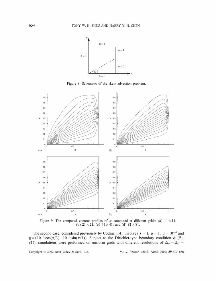
The second case, considered previously by Codina [14], involves f=1; R=1; �=10−4 andu=(10−4 cos(=3); 10−4 sin(=3)). Subject to the Dirichlet-type boundary condition � (�x∈@�), simulations were performed on uniform grids with di�erent resolutions of �x=�y=



1=10; 1=20; 1=40 and 1=80. Finite element results shown in Figure 6 reveal that sharp pro�lesof � could be captured without incurring oscillations.Another problem [18] was chosen to show the ability of the proposed �nite element model to

obtain oscillation-free solutions in a domain containing sharp layers. With �=10−8; u=(2; 3),and R=1, the source term f was properly chosen so as to render the exact solution givenbelow

�(x; y)=2y2 sin x[1− exp

(−2(1− x)�

)][1− exp

(−(1− y)�

)](34)

In the domain 0:996x61:0; 0:996y61:0, �nite element solutions were sought at four uni-form gird sizes: �x=�y=10−3=10; 10−3=20; 10−3=40 and 10−3=80. As in the previous test,the boundary layer pro�les shown in Figure 7 were obtained without incurring oscillations.For the sake of completeness, we also apply the presently developed monotonic CDR model

to solve for the skew advection problem [19], which has been frequently chosen to benchmarkthe discontinuity-capturing convection–di�usion models. In Figure 8, the dashed line, with theangle of (= tan−1 v=u==6), divides the unit cavity into two parts. The �ow condition underinvestigation is that with �=2× 10−4 and (u; v)= (√3=2; 12 ). It is seen from Figure 9 that nooscillation has been observed near the dividing line for each test grid. This demonstrates theability of the proposed model to resolve the interior sharp layer.

6. CONCLUDING REMARKS

We have presented in this paper the Petrov–Galerkin �nite element model for solving theconvection–di�usion-reaction equation in two dimensions. Our aim is to retain stability withoutreducing accuracy. To achieve this goal, we add a term to make the consistent �nite elementmodel into its inconsistent counterparts so as to eliminate three leading mixed derivatives.Good agreement with the smoothly varying exact solution has been obtained, thus verifyingthe applicability of the proposed �nite element model. We have also extended the �niteelement model based on the M -matrix theory and applied it to solve a problem involvinglarge gradients. Computations have demonstrated the model’s ability to capture sharply varyingpro�les near the boundary as well as in the �ow interior.

ACKNOWLEDGEMENTS

Financial support from the National Science Council of the Republic of China under Grant NSC88-2611-E-002-025 is acknowledged.

REFERENCES

1. Ilinca F, Pelletier D. Positivity preservation and adaptive solution for the k–� model of turbulence. AIAAJournal 1988; 36(1):44–50.

2. Crochet MJ, Davies AT, Walters K. Numerical Simulation of Non-Newtonian Flow. Elsevier: New York, 1984.3. Leboucher L. Monotone scheme and boundary conditions for �nite volume simulation of magnetohydrodynamicinternal �ows at high Hartmann number. Journal of Computational Physics 1999; 150:181–198.

4. Harari I, Hughes TJR. Finite element methods for the Helmholtz equation in an exterior domain: model problems.Computer Methods in Applied Mechanics and Engineering 1991; 87:59–96.



5. Ataie-Ashtini B, Lockington DA, Volker RE. Numerical correction of �nite di�erence solution of the advection–dispersion equation with reaction. Journal of Contaminant Hydrology 1996; 23:149–156.

6. Hossain MA. Modeling advective–dispersive transport with reaction: An accurate explicit �nite di�erence model.Applied Mathematics and Computation 1999; 102:101–108.

7. Hossain MA, Young DR. On Galerkin models for transport in groundwater. Applied Mathematics andComputation 1999; 100:249–263.

8. Harari I, Hughes TJR. Stabilized �nite element methods for steady advection–di�usion with production.Computer Methods in Applied Mechanics and Engineering 1994; 155:165–191.

9. Idelsohn S, Nigro N, Storti M, Buscaglia G. A Petrov–Galerkin formulation for advection–reaction-di�usionproblems. Computer Methods in Applied Mechanics and Engineering 1996; 136:27–46.

10. Uri M Ascher, Robert MM Mattheij, Robert D Russell. Numerical Solution of Boundary Value Problems forOrdinary Di�erential Equations. Prentice-Hall: New Jersey, 1998; 454–456.

11. Doolan EP, Miller JJH, Schilders WHA. Uniform Numerical Methods for Problems with Initial and BoundaryLayers. Boole Press: Dubin, 1980.

12. Tezdugar T, Park Y. Discontinuity capturing �nite element formulations for nonlinear convection–di�usion-reaction equations. Computer Methods in Applied Mechanics and Engineering 1986; 59:307–325.

13. Codina R. A chock-capturing anisotropic di�usion for the �nite element solution of the di�usion–convection-reaction equation. Finite Element in Fluids, New trends and Applications Part 1, Morgan K. (ed.), Pineridge:Swansea, 1993; 67–75.

14. Codina R. Comparison of some �nite element methods for solving the di�usion–convection–reaction equation.Computer Methods in Applied Mechanics and Engineering 1998; 156:185–210.

15. Warming RF, Hyette BJ. The modi�ed equation approach to the stability and accuracy analysis of �nite-di�erencemethods. Journal of Computational Physics 1974; 14:159–179.

16. Hughes TJR, Brooks AN. A multi-dimensional upwind scheme with no crosswind di�usion. In Finite ElementMethods for Convection Dominated Flows, Hughes TJR (ed.), AMD 34: ASME: New York, 1979; 19–35.

17. Meis T, Marcowitz U. Numerical solution of partial di�erential equations. In Applied Mathematical Science.John F, Sirovich L, La Salle JP (eds). Springer: Berlin, 1981; 32.

18. Lin� T, Stynes M. Numerical methods on shishkin meshes for linear convection–di�usion problems. ComputerMethods in Applied Mechanics and Engineering 2001; 190:3527–3542.

19. Gri�ths DF, Mitchell AR. In Finite Element for Convection Dominated Flows, Hughes TJR (ed.), in AMD34. ASME: New York, 1979; 91–104.


Documents

Amulti-dimensionalmonotonicniteelementmodelfor ...homepage.ntu.edu.tw/~twhsheu/member/paper/78-2002.pdfxx+R f=Ru x+ 4 −) 3 +u2 − h2R 6 xx+H:O:T: (12) isderivedsubjecttotheconsistencyrequirement