Ams96ppr

8/9/2019 Ams96ppr

http://slidepdf.com/reader/full/ams96ppr 1/4

9 AIRPOL FA P1.4 CLIMATRONICS’ NOVEL SONIC ANEMOMETER

John H. Robertson*

David I. Katz

Climatronics Corporation

Bohemia, New York

1. INTRODUCTION

Climatronics Corp. has developed a new sonic

anemometer utilizing a novel approach. This

anemometer fills the need for a rugged, compact, ice

free, non moving part anemometer. The resulting

anemometer is small, only 10 cm in diameter and 16 cm

long and has been designed to replace cup and vane or

propeller anemometers in most applications. Another

feature of the sensor is its’ low power consumption

requiring less than 0.5 watt for operation.

2. DESCRIPTION

Climatronics’ sonic anemometer’s operation is based on

the same classic principles as most sonic anemometers.

The time required for a sound wave to travel from point

A to point B is effected by the speed of the wind in a

predictable and repeatable way. The novel feature of

this anemometer is that the sound is directed down and

reflected from a second surface before being detected at

the receiver. This arrangement has the advantage that

the transducers are out of the weather and out of the

direct path of the wind which resulted in a very rugged

and compact design.

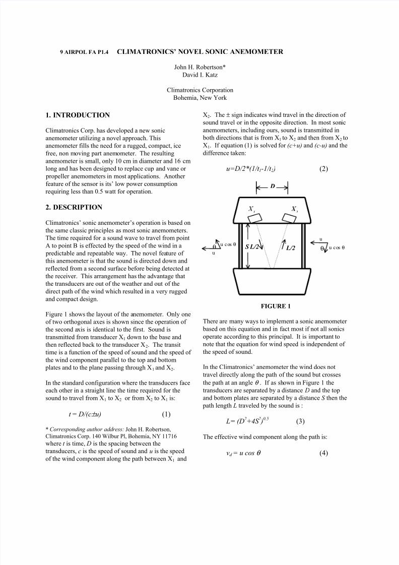
Figure 1 shows the layout of the anemometer. Only one

of two orthogonal axes is shown since the operation of

the second axis is identical to the first. Sound is

transmitted from transducer X1 down to the base and

then reflected back to the transducer X2. The transit

time is a function of the speed of sound and the speed of

the wind component parallel to the top and bottom

plates and to the plane passing through X1 and X2.

In the standard configuration where the transducers face

each other in a straight line the time required for the

sound to travel from X1 to X2 or from X2 to X1 is:

t = D/(c± u) (1)

* Corresponding author address: John H. Robertson,

Climatronics Corp. 140 Wilbur Pl, Bohemia, NY 11716

where t is time, D is the spacing between the

transducers, c is the speed of sound and u is the speed

of the wind component along the path between X1 and

X2. The ± sign indicates wind travel in the direction of

sound travel or in the opposite direction. In most sonic

anemometers, including ours, sound is transmitted in

both directions that is from X1 to X2 and then from X2 to

X1. If equation (1) is solved for (c+u) and (c-u) and the

difference taken:

u=D/2*(1/t 1-1/t 2 ) (2)

FIGURE 1

There are many ways to implement a sonic anemometer

based on this equation and in fact most if not all sonics

operate according to this principal. It is important to

note that the equation for wind speed is independent of

the speed of sound.

In the Climatronics’ anemometer the wind does not

travel directly along the path of the sound but crosses

the path at an angle θ . If as shown in Figure 1 the

transducers are separated by a distance D and the top

and bottom plates are separated by a distance S then the path length L traveled by the sound is :

L= (D2+4S

2 )

0.5(3)

The effective wind component along the path is:

vd = u cos θ (4)

L/2 L/2

D

2

1

u cos θθu cos θ

θ S

u

u

8/9/2019 Ams96ppr


If S is made very small θ approaches zero, cos θ

becomes unity and the path length L approaches D. In

other words the sensitivity is reduced by cos θ . A large

S minimizes interference with the wind field. At the

same time a large S reduces sensitivity because cos θ

becomes small. In the final instrument the values of S

and D are determined by such factors as desiredaccuracy, sensitivity, overall size, etc.

It is desirable to keep the spacing D small to achieve a

compact instrument. A compact instrument is rugged,

much easier to transport, install and de-ice. Having D

small leads to some problems. When D is small the

effective transit time is small and the effect of the delays

in the transducers and electronics can cause large errors.

In addition the actual transit time for the sound is long

because the sound must still travel over a distance of L.

It is possible to measure t 1-t 2 directly and this can

reduce some of these errors. A more complete

expression for the transit time, Schotland (1955) is:

t=D[(c2-vn2 )0.5

± vd ] / [c2-(vd 2+vn

2 )] + δ (5)

Where vn is the wind component normal to the

propagation path, c is the speed of sound, vd is the

component along the path and δ is the delay through the

transducers and electronics. If we assume that δ is the

same for both directions of propagation:

vd = (t 1-t 2 )[c2-(vd 2+vn

2 )] / 2D (6)

This expression not only requires that the speed of

sound is known but will require evaluation of (vd 2+vn2 ). The speed of sound can be approximated by:

c = [403T(1+0.32 e / P)]0.5 (7)

where T is the absolute temperature , e is the vapor

pressure and P is the barometric pressure. A reasonable

maximum value for e/P is 0.1 resulting in less then a

3% error in the speed of sound. The term (vd 2+vn

2 ) is

the velocity of the wind squared. At a speed of 50 m/s

the value of (6) is affected by less then 3% and at 20

m/s by less then 0.5%.

Setting (vd 2+vn

2 ) equal to zero and substituting c2 =403T results in:

vd = (t 1-t 2 )(403T) / 2D (8)

The assumption that the delay δ is equal is valid only

after careful matching of transducers and design of

electronics. Any mismatch results in offset and drift in

the instrument’s zero. In the present instrument these

errors are held to approximately ± 0.25 m/s.

One last potential source of error is the four posts used

to separate the upper and lower housings. These have

been made as small as possible and based on wind

tunnel testing have negligible effect on the wind flow.

The resulting anemometer is very simple and rugged.

In its simplest configuration a linear frequency

proportional to the speed along an axis is output for

each axis. In addition temperature is available as an

analog voltage. This information can be used to

calculate wind speed directly and if humidity and

pressure information are available the speed of sound

may be computed more accurately. In addition a

correction for the (vd 2+vn

2 ) term in equation (6) is

possible if additional accuracy is required.

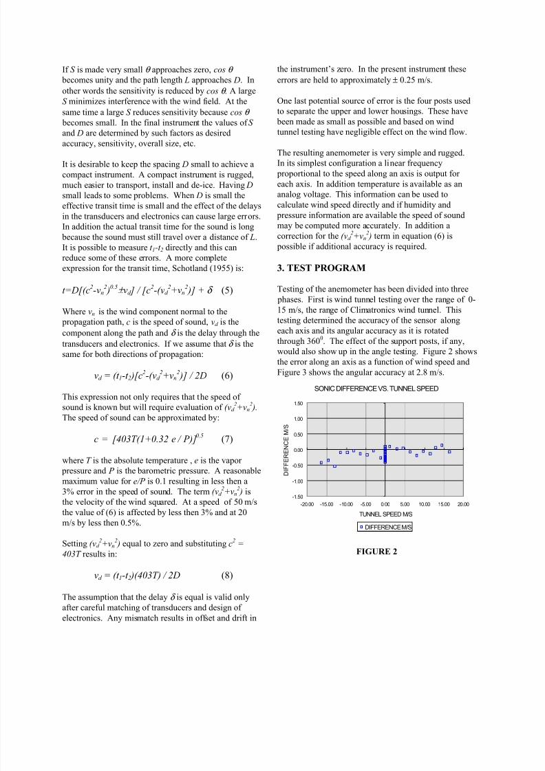
3. TEST PROGRAM

Testing of the anemometer has been divided into three

phases. First is wind tunnel testing over the range of 0-

15 m/s, the range of Climatronics wind tunnel. This

testing determined the accuracy of the sensor along

each axis and its angular accuracy as it is rotated

through 3600. The effect of the support posts, if any,

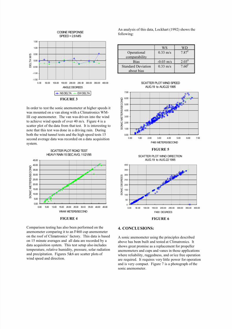
would also show up in the angle testing. Figure 2 shows

the error along an axis as a function of wind speed and

Figure 3 shows the angular accuracy at 2.8 m/s.

SONIC DIFFERENCE VS. TUNNEL SPEED

-1.50

-1.00

-0.50

0.00

0.50

1.00

1.50

-20.00 -15.00 -10.00 -5.00 0.00 5.00 10.00 15.00 20.00

TUNNEL SPEED M/S

D I F F E R E N C E M / S

DIFFERENCE M/S

FIGURE 2

8/9/2019 Ams96ppr


COSINE RESPONSE

SPEED = 2.8 M/S

-1.50

-1.00

-0.50

0.00

0.50

1.00

1.50

0.00 50.00 100.00 150.00 200.00 250.00 300.00 350.00 400.00

ANGLE DEGREES

D E L T A M

/ S

NS DELTA EW DELTA

FIGURE 3

In order to test the sonic anemometer at higher speeds it

was mounted on a van along with a Climatronics WM-

III cup anemometer. The van was driven into the wind

to achieve wind speeds of over 40 m/s. Figure 4 is a

scatter plot of the data from that test. It is interesting to

note that this test was done in a driving rain. During

both the wind tunnel tests and the high speed tests 15

second average data was recorded on a data acquisition

system.

SCATTER PLOT ROAD TEST

HEAVY RAIN 15 SEC AVG. 11/21/95

0.00

5.00

10.00

15.00

20.00

25.00

30.00

35.00

40.00

45.00

0.00 5.00 10.00 15.00 20.00 25.00 30.00 35.00 40.00 45.00

WM-III METERS/SECOND

S O N I C

M E T E R S / S E C

O N D

FIGURE 4

Comparison testing has also been performed on the

anemometer comparing it to an F460 cup anemometer on the roof of Climatronics’ factory. This data is based

on 15 minute averages and all data are recorded by a

data acquisition system. This test setup also includes

temperature, relative humidity, pressure, solar radiation

and precipitation. Figures 5&6 are scatter plots of

wind speed and direction.

An analysis of this data, Lockhart (1992) shows the

following:

WS WD

Operational

comparability

0.33 m/s 7.870

Bias -0.03 m/s 2.030

Standard Deviation

about bias

0.33 m/s 7.600

SCATTER PLOT WIND SPEED

AUG.19 to AUG.22 1995

0.00

1.00

2.00

3.00

4.00

5.00

6.00

7.00

0.00 1.00 2.00 3.00 4.00 5.00 6.00 7.00

F460 METERS/SECOND

S O N I C

M E T E R S / S E C O N D

FIGURE 5

SCATTER PLOT WIND DIRECTION

AUG.19 to AUG.22 1995

0

50

100

150

200

250

300

350

400

0.00 50.00 100.00 150.00 200.00 250.00 300.00 350.00 400.00

F460 DEGREES

S O N I C

D E G R E E S

FIGURE 6

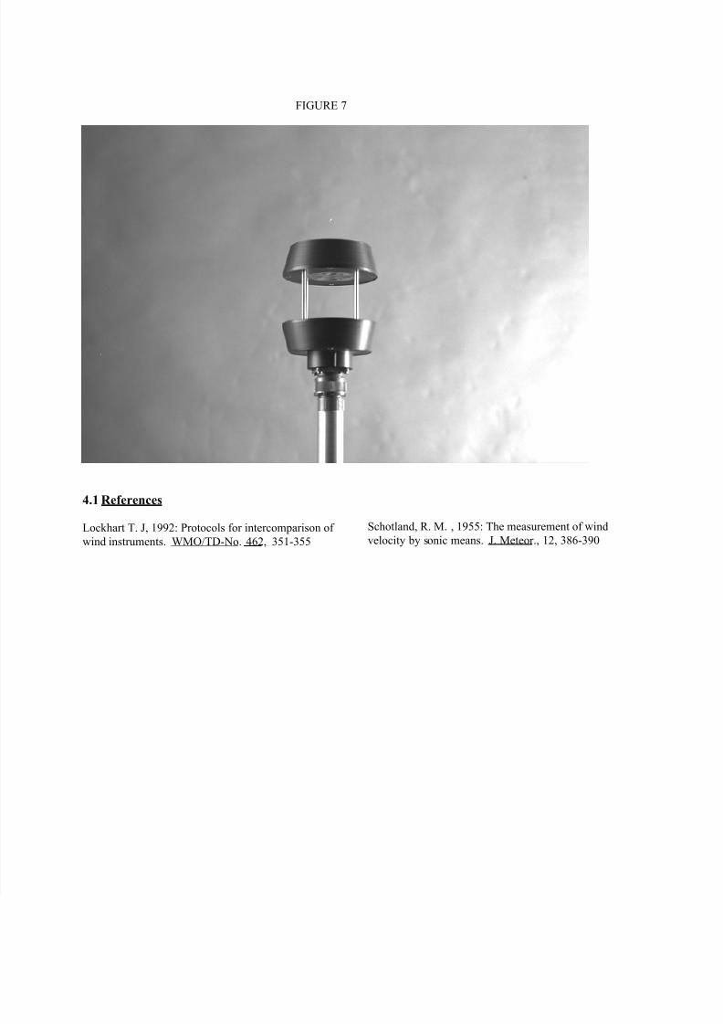
4. CONCLUSIONS:

A sonic anemometer using the principles described

above has been built and tested at Climatronics. It

shows great promise as a replacement for propeller

anemometers and cups and vanes in those applications

where reliability, ruggedness, and or/ice free operation

are required. It requires very little power for operation

and is very compact. Figure 7 is a photograph of the

sonic anemometer.

8/9/2019 Ams96ppr


FIGURE 7

4.1 References

Lockhart T. J, 1992: Protocols for intercomparison of

wind instruments. WMO/TD-No. 462, 351-355

Schotland, R. M. , 1955: The measurement of wind

velocity by sonic means. J. Meteor., 12, 386-390

Documents

Ams96ppr