Embed Size (px)
Citation preview
American Economic Association
An Experimental Investigation of the Patterns of International TradeAuthor(s): Charles N. Noussair, Charles R. Plott and Raymond G. RiezmanSource: The American Economic Review, Vol. 85, No. 3 (Jun., 1995), pp. 462-491Published by: American Economic AssociationStable URL: http://www.jstor.org/stable/2118183 .
Accessed: 03/03/2014 18:25
Your use of the JSTOR archive indicates your acceptance of the Terms & Conditions of Use, available at .http://www.jstor.org/page/info/about/policies/terms.jsp
.JSTOR is a not-for-profit service that helps scholars, researchers, and students discover, use, and build upon a wide range ofcontent in a trusted digital archive. We use information technology and tools to increase productivity and facilitate new formsof scholarship. For more information about JSTOR, please contact [email protected].
.
American Economic Association is collaborating with JSTOR to digitize, preserve and extend access to TheAmerican Economic Review.
http://www.jstor.org
This content downloaded from 131.215.23.238 on Mon, 3 Mar 2014 18:25:34 PMAll use subject to JSTOR Terms and Conditions
An Experimental Investigation of the Patterns of International Trade
By CHARLES N. NOUSSAIR, CHARLES R. PLOTT,
AND RAYMOND G. RIEZMAN *
This paper studies a laboratory economy with some of the prominent features of an international economic system. The patterns of trade and output predicted by the law of comparative advantage are observed evolving within the experimental markets. Market prices and quantities move in the direction of the competitive equilibrium, but the quantitative predictions of the (risk-neutral) competitive equilibrium are rejected. Considerable amounts of economic activity occur as disequilibria. Factor-price equalization is observed, but there is a universal tendency for factors of production to trade at prices below their marginal products. (JEL D50, FOO, F30)
This study is the first attempt to create and study a laboratory economy with some of the prominent features of an interna- tional economic system. The purpose is to investigate some of the economic profes- sion's fundamental assumptions about the nature of international trade. The concept of multiple "countries" in which each coun- try has its own technology, preferences, and resource endowments, is introduced and op- erationalized. The questions posed in the study are related to the law of comparative advantage, factor-price equalization, terms of trade, efficiency in production, and ex- change as guided by multiple and interact- ing markets and the effects of tariffs on international transactions. The study builds
on previous work in the experimental study of general equilibrium phenomena.'
Because this paper carries laboratory ex- perimental research to a new dimension of complexity and into a new field, it might be useful to address what would be the obvious concern of a skeptic. Since the world's in- ternational economies are vastly more com- plicated than the economies created for this study, of what relevance are laboratory-gen- erated data? The answer is that laboratory experiments are not attempts to simulate field situations, as that question of the skep- tic seems to presume. Laboratory research deals with the general theories and the gen- eral principles that are supposed to apply to all economies, the economies found in the field as well as those created in a labora- tory. The laboratory economies are very simple and are special cases of the broad class of (often complex) economies to which the general theories are supposed to be of relevance. If a general theory does not work successfully to explain behavior in the sim-
* Noussair: Department of Economics, Krannert School of Management, Purdue University, West Lafayette, IN 47907; Plott: Humanities and Social Sci- ences-m/c 228-77, California Institute of Technol- ogy, Pasadena, CA 91125; Riezman: Department of Economics, College of Business Administration, W210 PBAB, University of Iowa, Iowa City, IA 52242. We acknowledge the financial support of the National Sci- ence Foundation and the Caltech Laboratory for Ex- perimental Economics and Political Science. The com- ments of Charles Holt have been useful. The com- ments of Mahmoud El-Gamal were especially helpful and resulted in the econometric model used extensively in the paper.
1Jessica Goodfellow and Plott (1990) investigate the simultaneous determination of input and output prices. Peng Lian and Plott (1993), create a macroeconomy which includes one input and one output as well as fiat money and bonds.
462
This content downloaded from 131.215.23.238 on Mon, 3 Mar 2014 18:25:34 PMAll use subject to JSTOR Terms and Conditions
VOL. 85 NO. 3 NO USSA IR ETAL.: PATTERNS OF INTERNATIONAL TRADE 463
ple and special cases of the laboratory, then it is not general. When a model is found not working, opportunity exists to modify the theory to account for the data or to reject the theory. Thus, the laboratory provides an arena in which competing notions and theo- ries about the nature of human (and mar- ket) capacities can be joined with data. Clearly laboratory experimental work is constrained by technology, and by back- ground experimental work. When very little background work exists, the experimental research strategy is first to explore what seem to be the most basic and general theo- retical ideas. Then, as technology permits, successful ideas can be challenged with in- creasingly complex experimental environ- ments in follow-up experiments. Any labo- ratory experiment should be viewed as only one of the many steps needed to learn what we would like to know. This study is no different.
The focus of the study is the behavior of the entire economic system, rather than the behavior of individual agents. Two behav- ioral models, "competitive equilibrium" and "autarky," can be applied to the experimen- tal environments. Both models make precise predictions of the magnitude of every vari- able in the system, which number in the dozens. The existence of such a large num- ber of predictions creates methodological and expositional problems. With a large number of predictions, some predictions will almost certainly be wrong. The sheer size of the undertaking makes it very easy to reject the models statistically. Therefore, after making a clear statement of the negative result that the models are rejected, the analysis of the data focuses on the general properties of interdependent markets that are suggested by the models, as opposed to a focus on the accuracy of the specific pre- dictions of each model. In the context of the broad implications of the models, a number of results are stated.
The paper is organized in the following manner. We begin by discussing in Section I the existing support found in field data for the basic principles we test. In Sections II and III, the design of the experiments is described. In Section IV, the theoretical
models are discussed. In Section V, the data are presented and analyzed, and in Section VI, the conclusions are summarized.
I. Field-Data Support for Major Principles
The propositions that we propose to ex- plore are so basic to accepted theory and are applied so universally, that some might wonder why we would bother. Is it the case that the law of comparative advantage and the principle of factor-price equalization are well documented and not controversial? We think not. Nagging doubts linger because no direct evidence exists. Empirical results in support of the most basic principles of international-trade theory are clouded as they always are when the data are from field sources. As Michael P. Porter (1990 p. 12) writes, "Evidence hard to reconcile with factor comparative advantage is not difficult to find."
In his handbook chapter on testing trade theories, Alan Deardorff (1984) discusses the general problem of testing trade theo- ries using field data. He cites two types of problems. First, simple trade models omit important features of the world economy, so model specification is an inherent problem. For example, the models usually assume only two countries, and they typically ignore transport costs. On the other hand, field data are generated by countries trading with many other countries in a world in which transportation costs exist and are often thought to be important. The second gen- eral problem is that theories tend to be stated in terms of variables that are not observable, so that testing these theories directly with field data is not possible. An example is the theory of comparative advan- tage.
The theory of comparative advantage is a general theory which states that countries will export that good which has the lowest relative price in autarky. However, attempts to test and assess the theory have only been indirect. In principle, this theory cannot be tested directly with field data because con- ditions of autarky and thus autarky prices are rarely, if ever, observed. In order to cope with this problem, researchers have
This content downloaded from 131.215.23.238 on Mon, 3 Mar 2014 18:25:34 PMAll use subject to JSTOR Terms and Conditions
464 THE AMERICAN ECONOMIC REVIEW JUNE 1995
developed more specific models like the Ricardian and Heckscher-Ohlin models. The purpose of these models is to build theoretical relationships from observables, like labor productivity or endowments, that can be extended to nonobservables, like au- tarky prices, and then to use the latter as the benchmarks against which trade flows are measured. Thus, tests of the Ricardian model, or the Heckscher-Ohlin model, are actually joint tests of comparative advantage and the particular specification (i.e., the Ri- cardian model or the Heckscher-Ohlin model).
Unfortunately, these indirect tests have failed to distinguish between competing the- ories. For example, empirical tests of the Ricardian trade model (and the related law of comparative advantage) using field data date back to the early work of G. D. A. MacDougall (1951, 1952). His procedure was to look at U.S. and U.K. exports to third countries and to see whether the pattern of exports is explained by differences in the two countries' labor requirements. He found that the ratios of U.S. to U.K. exports and U.S. to U.K. labor productivity are highly correlated, which is consistent with the pre- dictions of the Ricardian model and, there- fore, suggests the operation of the law of comparative advantage. But, as observed by Deardorff, the tests fail to distinguish be- tween the Ricardian model and the Heckscher-Ohlin model, and as a result, the role and support for the law of comparative advantage remained unclear.
Thus, from the beginning there has not been a clear test of the comparative advan- tage that is so fundamental to theory. Simi- larly, there have been relatively few studies testing factor-price equalization theory. Al- fred Tovias (1982) and Hans Gremmen (1985) look at the EEC countries to see if there is evidence that factor prices converge as trade becomes freer within the EEC. Their results are quite mixed. They find periods in which factor prices seem to con- verge, but later, as the economies become more integrated, factor prices do not seem to be converging. A later paper by Manouchehr Mokhtari and Farhad Rassekh (1989) looks at a bigger sample of countries and gets more positive results. They con-
sider all of the OECD countries and use more sophisticated techniques. Their find- ings suggest that factor prices are converg- ing within the OECD if countries are prop- erly grouped into high-wage and low-wage countries. Furthermore, their evidence sug- gests that it is trade liberalization that ac- counts for much of this convergence. The evidence on factor-price equalization is far from conclusive.
The experimental data do not have many of the problems that are associated with field data. The experimental data are gener- ated by only two countries. Transportation costs are under the control of the experi- menter. The underlying structure is known. Variables unavailable in the field, like au- tarky prices, are known in the experiment. Factor prices can be observed under au- tarky and under free trade. In the field, neither can be observed. The field data on labor, for example, involves a great deal of aggregation across different types of labor. This means that one actually compares av- erage wages of a group of workers in one country with the average wage of a different group in another country. If there is much variation across countries in groups, or if these groups change over time, a bias is introduced which may affect the results. No such problems exist in experiments.
Of course, experimental data are gener- ated by much simpler economic environ- ments than those found in the field. The preconditions for the operations of the prin- ciples have been introduced by the experi- menters. The experiments are able to pro- vide some insights into how models, based on the basic principles, are able to organize the data, given that the situation is one in which the model can be meaningfully ap- plied. The experiment cannot, however, an- swer the equally important questions about the relative likelihood that nature has cre- ated a situation for which the parametric and institutional features of the model are relevant.
II. Experimental Design: Parameters
This section consists of a description of the market conditions within which the eco- nomic activity occurs. The description in-
This content downloaded from 131.215.23.238 on Mon, 3 Mar 2014 18:25:34 PMAll use subject to JSTOR Terms and Conditions
VOL. 85 NO. 3 NOUSSAIR ETAL.: PATTERNS OF INTERNATIONAL TRADE 465
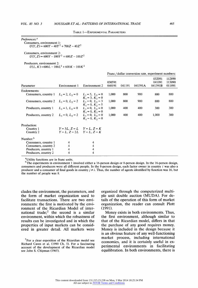
TABLE 1-EXPERIMENTAL PARAMETERS
Preferences:a Consumers, environment 1:
U(Y, Z) = 600Y - 40y2 + 700Z - 40Z2
Consumers, environment 2: U(Y, Z) = 600Y - 1O0y2 + 600Z - 10OZ2
Producers, environment 2: U(L, K) =600L - 100L2 + 600K - lOOK2
Franc/dollar conversion rate, experiment numbers:
032091 112890 030591 041091 113090
Parameter Environment 1 Environment 2 040191 041191 041391A 041391B 011891
Endowments: Consumers, country 1 L1 = 2, L2 = 0 L1 = 5, L2 = 0 1,000 800 900 800 800
K1=3, K2=0
Consumers, country 2 L1=O, L2= 2 L1 = 0, L2 = 3 1,000 800 900 800 800 K1 = O, K2 = 5
Producers, country 1 L1= 1, L2=0 L1 = 0, L2 =0 1,000 400 400 300 300 K1=O, K2=0
Producers, country 2 L1 = 0, L2 = 2 L1 = 0, L2 = 0 1,000 400 400 1,000 300 K1 = O, K2 = 0
Production: Countryl Y=3L, Z=L Y=L, Z=K Country2 Y=L, Z=2L Y=L, Z=K
Number:b Consumers, country 1 4 4 Consumers, country 2 4 4 Producers, country 1 4 4 Producers, country 2 4 4
aUtility functions are in franc units. bThe experiments in environment 1 involved either a 16-person design or 8-person design. In the 16-person design,
consumers and producers were all different people. In the 8-person design, each factor owner in country i was also a producer and a consumer of final goods in country j # i. Thus, the number of agents identified by function was 16, but the number of people was 8.
cludes the environment, the parameters, and the form of market organization used to facilitate transactions. There are two envi- ronments: the first is motivated by the envi- ronment of the Ricardian Model of inter- national trade;2 the second is a similar environment, within which the robustness of results can be investigated and in which the properties of input markets can be consid- ered in greater detail. All markets were
organized through the computerized multi- ple unit double auction (MUDA). For de- tails of the operation of this form of market organization, the reader can consult Plott (1991).
Money exists in both environments. Thus, the first environment, although similar to that of the Ricardian model, differs in that the purchase of any good requires money. Money is included in the design because it is an obvious feature of any well-functioning market process, including international economies, and it is certainly useful in ex- perimental environments in facilitating equilibration. In both environments, there is
2For a clear exposition of the Ricardian model see Richard Caves et al. (1990 Ch. 5). For a fascinating account of the development of the Ricardian model see John S. Chipman (1965).
This content downloaded from 131.215.23.238 on Mon, 3 Mar 2014 18:25:34 PMAll use subject to JSTOR Terms and Conditions
466 THE AMERICAN ECONOMIC REVIEW JUNE 1995
TABLE 2-REDEMPTION VALUES, ALL AGENTS, Two ENVIRONMENTS,
ONE COUNTRY (IDENTICAL COUNTRIES), ALL UNITS
Environment 1 Environment 2
Consumer Y Z Consumer Y Z Producer L K
1 600 620 1 600 450 1 600 450 520 540 250 400 250 400 440 480 200 50 200 50 360 400 280 320 2 550 500 2 550 500 200 240 300 350 300 350 120 160 150 100 150 100 40 80
2 560 660 3 500 550 3 500 550 480 580 350 300 350 300 400 500 100 150 100 150 320 420 4 450 600 4 450 600 240 340 400 250 400 250 180 260 50 200 50 200 100 180 20 100
20
3 560 660 480 580 400 500 320 420 240 340 180 260 100 180 20 100
20
4 520 700 440 620 360 540 280 460 200 380 120 300 40 220
140 60
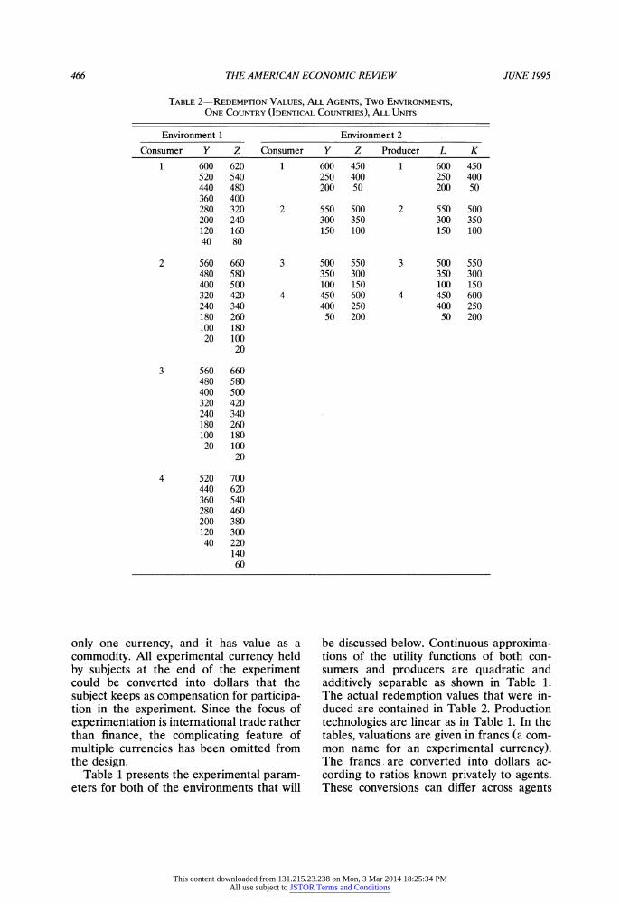
only one currency, and it has value as a commodity. All experimental currency held by subjects at the end of the experiment could be converted into dollars that the subject keeps as compensation for participa- tion in the experiment. Since the focus of experimentation is international trade rather than finance, the complicating feature of multiple currencies has been omitted from the design.
Table 1 presents the experimental param- eters for both of the environments that will
be discussed below. Continuous approxima- tions of the utility functions of both con- sumers and producers are quadratic and additively separable as shown in Table 1. The actual redemption values that were in- duced are contained in Table 2. Production technologies are linear as in Table 1. In the tables, valuations are given in francs (a com- mon name for an experimental currency). The francs. are converted into dollars ac- cording to ratios known privately to agents. These conversions can differ across agents
This content downloaded from 131.215.23.238 on Mon, 3 Mar 2014 18:25:34 PMAll use subject to JSTOR Terms and Conditions
VOL. 85 NO. 3 NOUSSAIR ETAL.: PATTERNS OF INTERNATIONAL TRADE 467
and are contained in Table 1. The variables Li and Ki refer to the factors L and K residing in country i and Yi and Zi refer to the outputs Y and Z produced in country i. The endowment listed in the table is the amount each individual agent possesses at the beginning of each market period. A country's total endowment is then four times the amount listed in the table, since each of the same type of agent has the same endow- ment.
A. Environment 1
Environment 1 is motivated by the Ricar- dian model. In environment 1, there are two output goods (final goods) called Y and Z and an input called L. There are two types of agents: consumers and producers. Con- sumers are owners of the factors of produc- tion and have induced preferences for con- suming the outputs Y and Z. Producers also have an initial endowment of the input and can earn profits by using the input L to produce and then sell Y and Z. All agents can also attempt to earn profits by speculat- ing in any input or output. Neither con- sumers nor producers have preferences for L other than its value as an input.
Agents are divided in equal numbers into two countries. Each country includes as members equal numbers of consumers and producers. The factor of production is not mobile between countries. The final goods Y and Z can be traded in either country, not only the one in which they were pro- duced. The two countries differ only in their production technologies.
The economy works in the following way. Consumers sell their endowment of L to producers in their own country and then buy units of Y and Z produced in either country. Consumers get utility (U.S. dollars) from consumption and any profits made in price speculation. Producers in each coun- try buy L from the consumers in their own country and can use L to produce Y and Z which they can sell to consumers in either country. Producers get utility (dollars) from profits earned from market and production activities.
In some experiments, free international trade was permitted; in others a tariff was
imposed on the imports of Z to country 1. When a tariff was in effect, it took the form of a tax of 400 francs on international trans- actions of the final goods. The tariff revenue was not redistributed to citizens in either country but instead was taken by the experi- menter. Thus, the tariff operated similarly to a transportation cost.
B. Environment 2
In environment 2, the two countries have different endowments of the inputs. In ad- dition, the inputs are endogenously and elastically supplied to producers in the sense that resources could also be con- sumed. Environment 2 operated as a con- trol on environment 1 to ensure that any properties of input markets observed in en- vironment 1 were not simply due to the completely inelastic supply of the input. The endogenous-resource property of environ- ment 2 is a natural feature to add as a check on robustness of a model's ability to capture observed behavior because it is a general property of the field economies in which the competitive and autarky models are regularly applied.
In environment 2 there are two output goods called Y and Z and two inputs called L and K. There are also two types of agents: consumers and producers. As in environ- ment 1, consumers are also owners of the factors of production. Consumers are en- dowed with some of both of the inputs L and K. Consumers have induced prefer- ences for consuming the outputs Y and Z. Producers of the final goods are also con- sumers of the factors of production. They have no initial endowment but have prefer- ences induced for consuming the inputs L and K and also for the money they might get by producing Y from L and Z from K and selling the output.
Participants are divided equally into two countries. Each country has an equal num- ber of consumers and producers. Both types of agents can trade the inputs L and K only with agents in their own country. The final goods Y and Z can be traded internation- ally. No tariffs existed in any of the experi- ments in which environment 2 was imple- mented.
This content downloaded from 131.215.23.238 on Mon, 3 Mar 2014 18:25:34 PMAll use subject to JSTOR Terms and Conditions
468 THE AMERICAN ECONOMIC REVIEW JUNE 1995
TABLE 3-SUMMARY OF EXPERIMENTS
Experiment Number of number (date) Tariffs Y/N Periods Environment Subject pool subjects
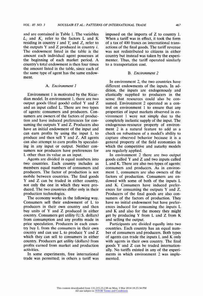
030591 N 11 1 Caltech 8 040191 N 10 1 Caltech 8 041191 N 9 1 U. Iowa 16 041391A N 10 1 U. Iowa (exper.)a 16 032091 Y 10 1 Caltech 8 041091 Y 9 1 U. Iowa 16 041391B Y 10 1 U. Iowa (exper.)a 8 112890 N 9 2 Caltech 16 113090 N 11 2 Caltech 16 011891 N 10 2 Caltech 16
aSubjects had experience in one of the earlier experiments listed here.
Consumers sell their endowment of in- puts to producers in their own country, and consumers buy units of Y and Z produced in either country. Producers can buy L and K from consumers in their own country. Producers can consume any part of the pur- chases of L and K and can use the remain- der to produce Y and Z, which they can then sell in either country.
III. Experimental Design: Procedures
A total of ten experiments were con- ducted. Table 3 provides a summary of treatments. Experiments are indexed by the date of the experiment. Two subject pools were used. The experiments involved either 8 people or 16 people. The use of 8 people for some experiments was dictated by cost and difficulties in recruiting subjects.
In the conditions of environments 1 and 2, there were six and eight markets, respec- tively, operating simultaneously.3 Each vari- able had its own market (e.g., output Yi, Y produced in country i, had its own market). The production process allowed subjects to transfer units from and to inventories of certain markets in fixed ratios. Production
was accomplished through a series of keystrokes. To consume units, subjects held them in their inventory at the end of a market period.
Subjects, undergraduates at the Califor- nia Institute of Technology and at the Uni- versity of Iowa, had at least one half hour of prior training in use of MUDA.4 The MUDA software is accompanied by a tuto- rial that explains the key functions to sub- jects and lets subjects practice using the keys in an environment containing randomly behaving robots. The Appendix contains in- structions read to subjects. During period 0 and period 1, accounting records were checked carefully for mistakes, and spot checks were conducted in later periods.
The experiment was divided into trading periods or trading "days." At the beginning of each, subjects received new endowments and redemption values which were the same each period. At the beginning of the experi- ment there was a long practice period (period 0) for 15 minutes in which no money was paid. Market periods averaged 10 min- utes in length.
3The names L and K were not used to label the markets in any experiments because they might suggest behavior to the subjects if they thought that L and K represented labor and capital. The labels used in mar- kets are explained in the Appendix.
Although Caltech subjects were only allowed to participate in one experiment in this particular line of experimentation, some of the Caltech subjects had been in other market experiments. None of the Univer- sity of Iowa subjects had been in other market experi- ments previously, although experiments 041391A and 041391B used only subjects who had been in one of the previous experiments in the series.
This content downloaded from 131.215.23.238 on Mon, 3 Mar 2014 18:25:34 PMAll use subject to JSTOR Terms and Conditions
VOL. 85 NO. 3 NOUSSAIR ETAL.: PATTERNS OF INTERNATIONAL TRADE 469
IV. Models
The models described below rely on strong assumptions. The complex environ- ments of the experimental markets are much richer than those that the models describe. However, experimental economics has demonstrated that models frequently have surprising power even when applied to envi- ronments much more complex than the structure of the models. The questions that will ultimately be posed concern the identi- fication of models that can provide intuition needed for help with the interpretation of market data.
A. The Competitive Model
This section contains a brief elaboration and review of the competitive model. The computation and description of the compet- itive equilibria for both environments are in a technical appendix which is available from the authors upon request. Recall that the first environment has two outputs, both of which can be produced with the same input, paralleling that of the Ricardian model of international trade. In the Ricardian envi- ronment there are two final goods, Y and Z, each of which is produced using one factor, L. There are two countries which may differ in their endowments of the factor. The fac- tor cannot cross national boundaries and is supplied inelastically to the markets. The two countries are assumed to have different production functions so that each country has a comparative advantage in production of one of the goods. Without loss of gener- ality, call the country with a comparative advantage in the production of Y country 1. The two countries have identical aggregate demand for both goods. In autarky, the price ratio Pz/Py should be greater in country 1 than in country 2. That is, country 1 can produce good Y more cheaply in terms of good Z then can country 2. If trade between the two countries is permitted, then comparative advantage dictates that country 1 specializes in and exports good Y. Simi- larly, country 2 specializes in and exports good Z. If the final goods are traded with- out restrictions, the prices of the final goods,
Y and Z, will be the same across countries and the price of L generally will be different in each country.
Thus, for environment 1, the competitive model predicts that countries 1 and 2 would produce exclusively goods Y and Z, respec- tively, and that each of the two countries would be a net exporter of the output which it produces. In particular country 1 would produce only Y, and country 2 would pro- duce only Z. The prices of the outputs would be equal in each country according to the model, and the prices of inputs would equal their marginal revenue products.
If a tariff were imposed on the country-1 imports of Z in environment 1, then accord- ing to the competitive model international trade of Z would decline. The price of Z in country 1 would increase, and the price of Z in country 2 would fall. The input price in country 2 would also decline, since its marginal revenue product would be lower. The tariff imposed was 400 francs.
In environment 2, the competitive model predicts that each country would produce both output goods. Country 1, however, would be a net exporter of Y, and country 2 would be a net exporter of Z. Under condi- tions of free trade, the prices of outputs would be equal across countries. Since de- rived demand would be identical in both countries, then the factor prices would also be the same and would equal the factors' marginal revenue product. The price of each of the four types of goods in country 1 would equal its price in country 2. The prediction of the equality of input prices across countries in environment 2 will be referred to as the factor-price equalization principle. Notice that for the parameter val- ues imposed in this environment, factor- price equalization is predicted even though the factors cannot be traded internationally.
B. Autarky
A natural alternative model to use is the autarky model. It is useful because it char- acterizes one benchmark of the potential behavior which a system might exhibit. Its predictions are based upon the proposition that no trade will occur across national
This content downloaded from 131.215.23.238 on Mon, 3 Mar 2014 18:25:34 PMAll use subject to JSTOR Terms and Conditions
470 THE AMERICAN ECONOMIC REVIEW JUNE 1995
TABLE 4-SPECIFIC PREDICTIONS OF THE Two MODELS: PRODUCTION AND EXPORT QUANTITIES AND PRICES
IN FRANCS WITH AND WITHOUT TARIFFS
Environment 1
Competitive Autarky Environment 2
With No With No Variable tariff tariff tariff tariff Competitive Autarky
Production: Y, 36 36 21 21 12 10 Y2 0 0 5 5 4 6 Z, 0 0 5 5 4 6 Z2 32 32 22 22 12 10
Exports: Y, 18 18 0 0 4 0 Y2 0 0 0 0 0 0
Net Y (from 1 to 2) 18 18 0 0 4 0 Z1 0 0 0 0 0 0 Z2 16 6 0 0 4 0 Net Z(from 2 to l) 16 6 0 0 4 0
Prices: L, 720 720 600 600 200-250 150 L2 760 360 520 520 200-250 300-350 K1 200-250 300-350 K2 200-250 150 Y, 240 240 200 200 200-225 150 Y2 520 520 200-225 300-350 Z1 600 600 200-225 300-350 Z2 380 180 260 260 200-225 150
boundaries. This model predicts the prices and production levels in each country which would occur in a competitive equilibrium with no international transactions permit- ted. This model thus offers specific predic- tions of prices, patterns of production, in- ternational trade, and the effects of tariffs.
For environment 1, the autarky model predicts that specialization would not occur in either country, and that there would be no international trade or payment imbal- ances. Since there is no trade across na- tional boundaries, the predictions of this model are unaffected by the imposition of tariffs. According to the autarky model, prices of all goods would be different in the two countries.
The autarky model also makes predic- tions concerning production and trade in the two countries in environment 2. Both countries produce both goods but in differ- ent quantities than in the competitive equi- librium. Autarky predicts that there will be
no international trade and that both input and output prices will be different across countries. The wage-price ratio predictions are identical to those predicted by the com- petitive model. There should be no payment imbalances. The predictions of the autarky model are computed in a similar way to the competitive model. The computations are available from the authors upon request.
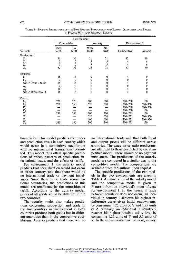
The specific predictions of the two mod- els in the two environments are given in Table 4. An illustration of the autarky model and the competitive model is given in Figure 1 from an individual's point of view for environment 1. In the figure, if trade between countries does not occur, an indi- vidual in country 1 achieves his highest in- difference curve given initial endowments, by consuming 5.25 units of Y and 1.25 units of Z. Similarly, an individual in country 2 reaches his highest possible utility level by consuming 1.25 units of Y and 5.5 units of Z. In the experimental environment, money,
This content downloaded from 131.215.23.238 on Mon, 3 Mar 2014 18:25:34 PMAll use subject to JSTOR Terms and Conditions
VOL. 85 NO. 3 NOUSSAIR ETAL.: PATTERNS OF INTERNATIONAL TRADE 471
which has value to all agents, may be bor- rowed costlessly in large quantities from the experimenter. For this reason, there is no budget constraint. The optimal consump- tion bundle is determined by the prices of Y and Z and by the consumer's utility for Y, Z, and money. The autarky consumption bundles of individual consumers in the two countries are labeled with A's in the figure. If free trade occurs, then each country can achieve a higher utility level by specializing in the commodity in which it has a compara- tive advantage and then trading internation- ally at the world competitive equilibrium price. The competitive-equilibrium individ- ual consumption bundles are labelled with C's. In the competitive equilibrium, each country consumes 18 units of Y and 16 units of Z.
C. Efficiency
The efficiency measurements in our ex- periments were first developed by Plott and Smith (1978). In a single market the system is operating at 100-percent efficiency if the total profit that all subjects make in an experiment is at a maximum. It is similar to maximizing consumer plus producer sur- plus.
In a general-equilibrium system the prob- lem becomes a little tricky. Because of the single currency in these experiments, the gains from exchange are exhausted at the maximum of system profits in terms of the experimental currency, francs. Actual profits divided by the maximum possible becomes the measure of system efficiency. Efficiency is 100 percent if the competitive equilibrium is attained. When tariffs were imposed, the government revenues were treated the same as were the profits of individuals and, therefore, included as part of the "consumer surplus" that was created by exchange.
V. Results
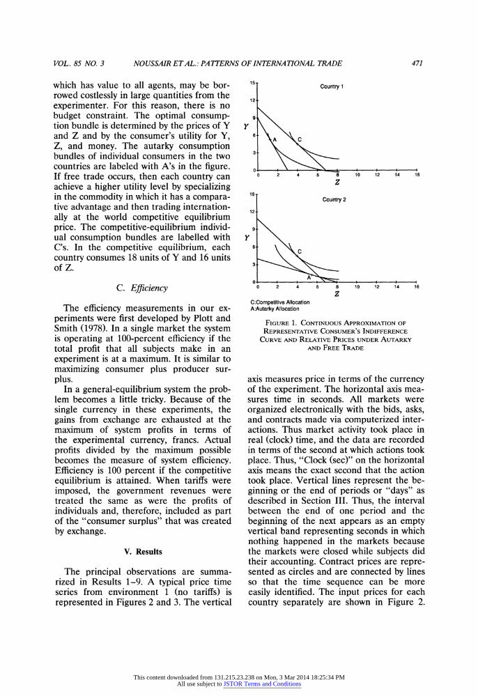
The principal observations are summa- rized in Results 1-9. A typical price time series from environment 1 (no tariffs) is represented in Figures 2 and 3. The vertical
15- Country 1
12 .
9.
6 A C
3
0 2 4 6 8 10 12 14 16
z
15
Country 2
12
9
6-
3-
0. 0 2 4 6 8 10 12 14 16
z
C:Competitive Allocation A:Autarky Allocation
FIGURE 1. CONTINUOUS APPROXIMATION OF
REPRESENTATIVE CONSUMER'S INDIFFERENCE
CURVE AND RELATIVE PRICES UNDER AUTARKY
AND FREE TRADE
axis measures price in terms of the currency of the experiment. The horizontal axis mea- sures time in seconds. All markets were organized electronically with the bids, asks, and contracts made via computerized inter- actions. Thus market activity took place in real (clock) time, and the data are recorded in terms of the second at which actions took place. Thus, "Clock (sec)" on the horizontal axis means the exact second that the action took place. Vertical lines represent the be- ginning or the end of periods or "days" as described in Section III. Thus, the interval between the end of one period and the beginning of the next appears as an empty vertical band representing seconds in which nothing happened in the markets because the markets were closed while subjects did their accounting. Contract prices are repre- sented as circles and are connected by lines so that the time sequence can be more easily identified. The input prices for each country separately are shown in Figure 2.
This content downloaded from 131.215.23.238 on Mon, 3 Mar 2014 18:25:34 PMAll use subject to JSTOR Terms and Conditions
472 THE AMERICAN ECONOMIC REVIEW JUNE 1995
floo
Competitive_Equilibrium r5z
6001 ~ ~ ~ -~ Autarky
0.000) _ _ - - - - - - - -
23.0 304 1584 2365 3145 3926 4706 547 6267 7048 7828 360
Clock(sec)
1000
i001__ X Competitive Equllibium 1l ll l
400104 +0t 2001
* 23.0 804 1584 2365 3145 3926 4706 5487 6267 7048 7828 8609 Ctock(sec)
FIGURE 2. INPUT-PRICE TIME SERIES, EXPERIMENT 041391A: COUNTRY 1 (UPPER GRAPH) AND
COUNTRY 2 (LOWER GRAPH)
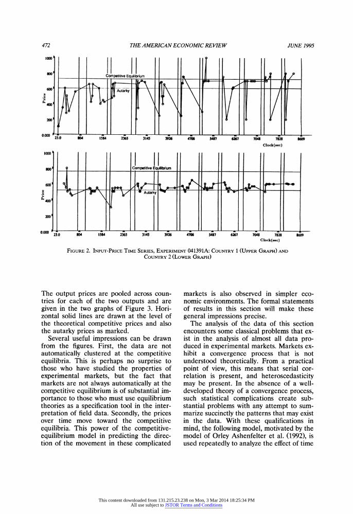
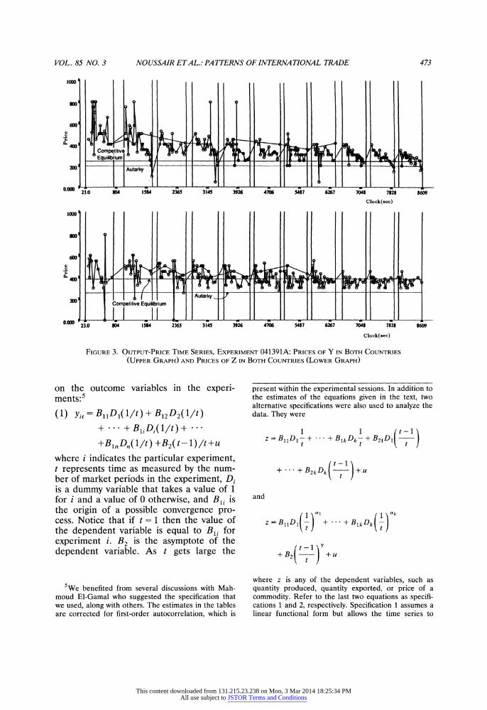
The output prices are pooled across coun- tries for each of the two outputs and are given in the two graphs of Figure 3. Hori- zontal solid lines are drawn at the level of the theoretical competitive prices and also the autarky prices as marked.
Several useful impressions can be drawn from the figures. First, the data are not automatically clustered at the competitive equilibria. This is perhaps no surprise to those who have studied the properties of experimental markets, but the fact that markets are not always automatically at the competitive equilibrium is of substantial im- portance to those who must use equilibrium theories as a specification tool in the inter- pretation of field data. Secondly, the prices over time move toward the competitive equilibria. This power of the competitive- equilibrium model in predicting the direc- tion of the movement in these complicated
markets is also observed in simpler eco- nomic environments. The formal statements of results in this section will make these general impressions precise.
The analysis of the data of this section encounters some classical problems that ex- ist in the analysis of almost all data pro- duced in experimental markets. Markets ex- hibit a convergence process that is not understood theoretically. From a practical point of view, this means that serial cor- relation is present, and heteroscedasticity may be present. In the absence of a well- developed theory of a convergence process, such statistical complications create sub- stantial problems with any attempt to sum- marize succinctly the patterns that may exist in the data. With these qualifications in mind, the following model, motivated by the model of Orley Ashenfelter et al. (1992), is used repeatedly to analyze the effect of time
This content downloaded from 131.215.23.238 on Mon, 3 Mar 2014 18:25:34 PMAll use subject to JSTOR Terms and Conditions
VOL. 85 NO. 3 NOUSSAIR ETAL.: PATTERNS OF INTERNATIONAL TRADE 473
4000
600
Com petitve Eqibru
0 23.0 804 1584 2365 3145 3926 4706 5487 6267 7048 7828 8609
Clock(sec)
: j F T m n- T | ~~~~~Autarky
OOOD Jt 1 Competitive Equilibrum 1lI ll ll ll *.0 23.0 804 1594 2365 31r45 3926 4706 S487 6267 7048 7828 8609
Clock( sec)
FIGURE 3. OUTPUT-PRICE TIME SERIES, EXPERIMENT 041391A: PRICES OF Y IN BOTH COUNTRIES
(UPPER GRAPH) AND PRICES OF Z IN BOTH COUNTRIES (LOWER GRAPH)
on the outcome variables in the experi- ments:5
(1) yit = B11Dj(1/t) + B12D2(1/t) + * * * + BiA D1( 1/t ) +
+BlnDn(llt) +B2( t-l)/t+u
where i indicates the particular experiment, t represents time as measured by the num- ber of market periods in the experiment, Di is a dummy variable that takes a value of 1 for i and a value of 0 otherwise, and Bli is the origin of a possible convergence pro- cess. Notice that if t = 1 then the value of the dependent variable is equal to Bli for experiment i. B2 is the asymptote of the dependent variable. As t gets large the
5We benefited from several discussions with Mah- moud El-Gamal who suggested the specification that we used, along with others. The estimates in the tables are corrected for first-order autocorrelation, which is
present within the experimental sessions. In addition to the estimates of the equations given in the text, two alternative specifications were also used to analyze the data. They were
1 1 t z = B11D1- + + BlkDk- + B21D1 ()
t t
+ + B2kDk ( t + u
and
1a, ak
z= B11D,t + **+ BlkDk(|)
+ B2 + u 2 t
where z is any of the dependent variables, such as quantity produced, quantity exported, or price of a commodity. Refer to the last two equations as specifi- cations 1 and 2, respectively. Specification 1 assumes a linear functional form but allows the time series to
This content downloaded from 131.215.23.238 on Mon, 3 Mar 2014 18:25:34 PMAll use subject to JSTOR Terms and Conditions
474 THE AMERICAN ECONOMIC REVIEW JUNE 1995
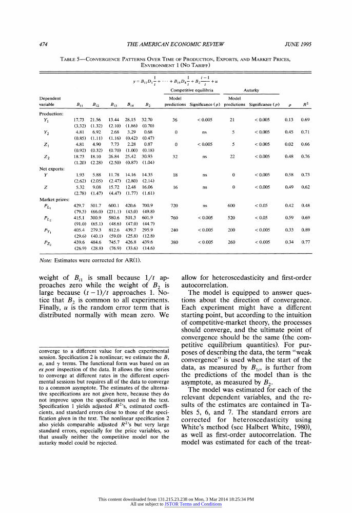
TABLE 5-CONVERGENCE PATTERNS OVER TIME OF PRODUCrION, EXPORTS, AND MARKET PRICES, ENVIRONMENT 1 (No TARIFF)
1 1 t-1 y=B11D1-+ +B14D4- +B2 ? +u
t t I
Competitive equilibria Autarky
Dependent Model Model variable BI1 B12 B13 B14 B2 predictions Significance (p) predictions Significance (p) p R2
Production:
Y, 17.73 21.56 13.44 28.15 32.70 36 < 0.005 21 < 0.005 0.13 0.69 (3.32) (1.32) (2.10) (1.86) (0.70)
Y2 4.81 6.92 2.68 3.29 0.68 0 ns 5 < 0.005 0.45 0.71 (0.85) (1.11) (1.16) (0.42) (0.47)
Z, 4.81 4.90 7.73 2.28 0.87 0 < 0.005 5 < 0.005 0.02 0.66 (0.92) (0.32) (0.70) (1.00) (0.18)
Z2 18.73 18.10 26.84 25.42 30.93 32 ns 22 < 0.005 0.48 0.76 (1.20) (2.28) (2.50) (0.87) (1.04)
Net exports: Y 1.93 5.88 11.78 14.16 14.35 18 ns 0 < 0.005 0.58 0.73
(2.62) (2.05) (2.47) (2.80) (2.14) Z 5.32 9.08 15.72 12.48 16.06 16 ns 0 < 0.005 0.49 0.62
(2.78) (1.47) (4.47) (1.77) (1.61) Market prices:
PLI 429.7 501.7 600.1 420.6 700.9 720 ns 600 < 0.05 0.42 0.48 (79.3) (66.0) (231.1) (43.0) (49.8)
PL2 415.1 300.9 580.6 501.3 601.9 760 < 0.005 520 < 0.05 0.59 0.69 (91.0) (65.1) (48.6) (47.0) (44.7)
Py, 405.4 279.3 812.6 439.7 295.9 240 < 0.005 200 < 0.005 0.33 0.89 (29.6) (40.1) (59.0) (25.8) (12.8)
PZ2 439.6 484.6 745.7 426.8 439.6 380 < 0.005 260 < 0.005 0.34 0.77 (26.9) (28.8) (76.9) (33.6) (14.6)
Note: Estimates were corrected for AR(1).
weight of Bil is small because 1/t ap- proaches zero while the weight of B2 is large because (t-1)/t approaches 1. No- tice that B2 is common to all experiments. Finally, u is the random error term that is distributed normally with mean zero. We
allow for heteroscedasticity and first-order autocorrelation.
The model is equipped to answer ques- tions about the direction of convergence. Each experiment might have a different starting point, but according to the intuition of competitive-market theory, the processes should converge, and the ultimate point of convergence should be the same (the com- petitive equilibrium quantities). For pur- poses of describing the data, the term "weak convergence" is used when the start of the data, as measured by B1i, is further from the predictions of the model than is the asymptote, as measured by B2.
The model was estimated for each of the relevant dependent variables, and the re- sults of the estimates are contained in Ta- bles 5, 6, and 7. The standard errors are corrected for heteroscedasticity using White's method (see Halbert White, 1980), as well as first-order autocorrelation. The model was estimated for each of the treat-
converge to a different value for each experimental session. Specification 2 is nonlinear; we estimate the B, a, and y terms. The functional form was based on an ex post inspection of the data. It allows the time series to converge at different rates in the different experi- mental sessions but requires all of the data to converge to a common asymptote. The estimates of the alterna- tive specifications are not given here, because they do not improve upon the specification used in the text. Specification 1 yields adjusted R2's, estimated coeffi- cients, and standard errors close to those of the speci- fication given in the text. The nonlinear specification 2 also yields comparable adjusted R2's but very large standard errors, especially for the price variables, so that usually neither the competitive model nor the autarky model could be rejected.
This content downloaded from 131.215.23.238 on Mon, 3 Mar 2014 18:25:34 PMAll use subject to JSTOR Terms and Conditions
VOL. 85 NO. 3 NO USSAIR ETAL.: PATTERNS OF INTERNATIONAL TRADE 475
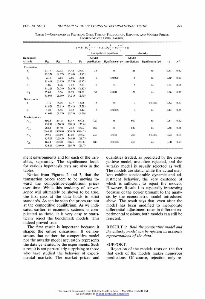
TABLE 6-CONVERGENCE PATTERNS OVER TIME OF PRODUCTION, EXPORTS, AND MARKET PRICES, ENVIRONMENT 1 (WITH TARIFFS)
1 1 t-1 y = B11D1 -+ + B13D3-+ B2- + u
t t
Competitive equilibria Autarky
Dependent Model Model variable BI1 B12 B13 B2 predictions Significance (p) predictions Significance (p) p R2
Production:
Y, 27.17 32.33 14.42 27.97 36 ns 21 ns 0.61 0.62 (3.37) (4.67) (5.48) (5.45)
Y2 2.13 9.14 9.56 3.96 0 < 0.005 5 ns 0.40 0.63 (1.41) (0.93) (2.23) (0.87)
Z, 3.06 1.26 7.03 2.57 0 ns 5 ns 0.64 0.66 (1.22) (1.74) (1.67) (1.82)
Z2 25.60 5.56 11.79 24.51 32 < 0.01 22 ns 0.56 0.77 (1.94) (1.99) (4.31) (2.70)
Net exports: Y 7.16 14.05 -1.77 13.06 18 ns 0 < 0.005 0.52 0.57
(1.82) (5.11) (3.41) (3.28) Z 1.23 1.85 0.72 1.42 6 < 0.005 0 ns 0.43 0.31
(1.03) (1.57) (0.75) (1.20) Market prices:
PL1 500.8 391.5 413.7 677.5 720 ns 600 ns 0.51 0.42 (56.9) (130.5) (68.1) (75.6)
PL2 268.4 247.0 -24.3 473.3 360 ns 520 ns 0.88 0.68 (646.5) (959.9) (938.2) (964.5)
PY, 297.9 1,002.9 434.0 289.2 240 < 0.01 200 < 0.005 0.22 0.84 (37.0) (103.5) (48.4) (18.7)
Pz2 166.4 1,003.0 606.5 283.6 180 < 0.005 260 ns 0.00 0.73 (38.1) (140.6) (95.7) (21.7)
ment environments and for each of the vari- ables, separately. The significance levels for various hypothesis tests are also in the tables.
Notice from Figures 2 and 3, that the transaction prices seem to be moving to- ward the competitive-equilibrium prices over time. While this tendency of conver- gence will ultimately be shown to be true, the first pass at the data holds to strict standards. As can be seen the prices are not at the competitive equilibrium. As we indi- cated earlier, in economic systems as com- plicated as these, it is very easy to statis- tically reject the benchmark models. This indeed proved true.
The first result is important because it shapes the entire discussion. It demon- strates that neither the competitive model nor the autarky model accurately represents the data generated by the experiments. Such a result is not particularly surprising to those who have studied the behavior of experi- mental markets. The market prices and
quantities traded, as predicted by the com- petitive model, are often rejected, and the autarky model is usually rejected as well. The models are static, while the actual mar- kets exhibit considerable dynamic and ad- justment behavior, the very existence of which is sufficient to reject the models. However, Result 1 is especially interesting because of the power brought to the analy- sis by the econometric model introduced above. The result says that, even after the model has been modified to incorporate differential adjustment rates in different ex- perimental sessions, both models can still be rejected.
RESULT 1: Both the competitive model and the autarky model can be rejected as accurate representations of the data.
SUPPORT: Rejection of the models rests on the fact
that each of the models makes numerous predictions. Of course, rejection only re-
This content downloaded from 131.215.23.238 on Mon, 3 Mar 2014 18:25:34 PMAll use subject to JSTOR Terms and Conditions
476 THE AMERICAN ECONOMIC REVIEW JUNE 1995
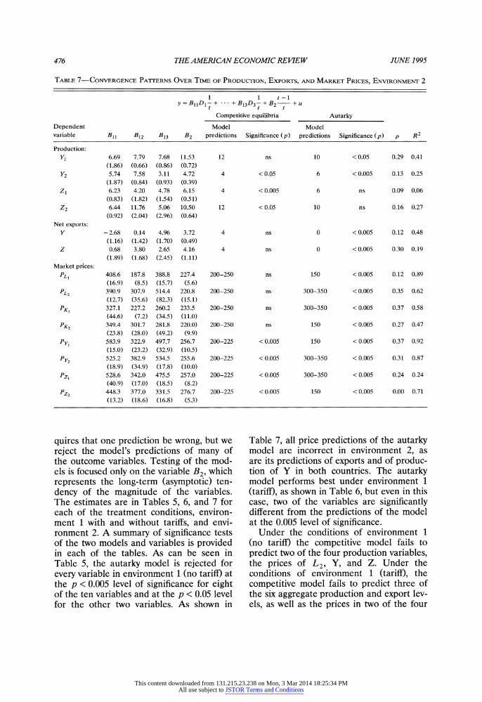
TABLE 7-CONVERGENCE PATTERNS OVER TIME OF PRODUCTION, EXPORTS, AND MARKET PRICES, ENVIRONMENT 2
1 1 t-1 y = B11D1- + +B13D3- +B2 +u
t t
Competitive equilibria Autarky
Dependent Model Model variable B11 B12 B13 B2 predictions Significance (p) predictions Significance (p) p R2
Production:
Y, 6.69 7.79 7.68 11.53 12 ns 10 < 0.05 0.29 0.41 (1.86) (0.66) (0.86) (0.72)
Y2 5.74 7.58 3.11 4.72 4 < 0.05 6 < 0.005 0.13 0.25 (1.87) (0.84) (0.93) (0.39)
Z, 6.23 4.20 4.78 6.15 4 < 0.005 6 ns 0.09 0.06
(0.83) (1.82) (1.54) (0.51)
Z2 6.44 11.76 5.06 10.50 12 < 0.05 10 ns 0.16 0.27
(0.92) (2.04) (2.96) (0.64)
Net exports: Y -2.68 0.14 4.96 3.72 4 ns 0 < 0.005 0.12 0.48
(1.16) (1.42) (1.70) (0.49) Z 0.68 3.80 2.65 4.16 4 ns 0 < 0.005 0.30 0.19
(1.89) (1.68) (2.45) (1.11) Market prices:
PLI 408.6 187.8 388.8 227.4 200-250 ns 150 < 0.005 0.12 0.89 (16.9) (8.5) (15.7) (5.6)
PL2 390.9 307.9 514.4 220.8 200-250 ns 300-350 < 0.005 0.35 0.62 (12.7) (35.6) (82.3) (15.1)
PK, 327.1 227.2 260.2 233.5 200-250 ns 300-350 < 0.005 0.37 0.58 (44.6) (7.2) (34.5) (1 1.0)
PK2 349.4 301.7 281.8 220.0) 200-250 ns 150 < 0.005 0.27 0.47 (23.8) (28.0) (49.2) (9.9)
Py, 583.9 322.9 497.7 256.7 200-225 < 0.005 150 < 0.005 0.37 0.92 (15.0) (23.2) (32.9) (10.5)
P Y2 525.2 382.9 534.5 255.6 200-225 < 0.005 300-350 < 0.005 0.31 0.87 (18.9) (34.9) (17.8) (10.0)
Pzl 528.6 342.0 475.5 257.0 200-225 < 0.005 300-350 < 0.005 0.24 0.24
(40.9) (17.0) (18.5) (8.2)
Pz2 448.3 377.0 331.5 276.7 200-225 < 0.005 150 < 0.005 0.00 0.71 (13.2) (18.6) (16.8) (5.3)
quires that one prediction be wrong, but we reject the model's predictions of many of the outcome variables. Testing of the mod- els is focused only on the variable B2, which represents the long-term (asymptotic) ten- dency of the magnitude of the variables. The estimates are in Tables 5, 6, and 7 for each of the treatment conditions, environ- ment 1 with and without tariffs, and envi- ronment 2. A summary of significance tests of the two models and variables is provided in each of the tables. As can be seen in Table 5, the autarky model is rejected for every variable in environment 1 (no tariff) at the p < 0.005 level of significance for eight of the ten variables and at the p < 0.05 level for the other two variables. As shown in
Table 7, all price predictions of the autarky model are incorrect in environment 2, as are its predictions of exports and of produc- tion of Y in both countries. The autarky model performs best under environment 1 (tariff), as shown in Table 6, but even in this case, two of the variables are significantly different from the predictions of the model at the 0.005 level of significance.
Under the conditions of environment 1 (no tariff) the competitive model fails to predict two of the four production variables, the prices of L2, Y, and Z. Under the conditions of environment 1 (tariff), the competitive model fails to predict three of the six aggregate production and export lev- els, as well as the prices in two of the four
This content downloaded from 131.215.23.238 on Mon, 3 Mar 2014 18:25:34 PMAll use subject to JSTOR Terms and Conditions
VOL. 85 NO. 3 NOUSSAIR ETAL.: PATTERNS OF INTERNATIONAL TRADE 477
markets. In all cases, the significance level supporting rejection is at least 0.05. As for environment 2, the competitive model is rejected for seven of the 14 variables at the 0.05 level of significance.
It is important to note, as is clear from the tables, that the competitive model has some merit when one compares the coeffi- cients B1i to B2. The remaining results are attempts to summarize those aspects of the competitive and autarky models that are successful. The general theme is that con- vergence of the data over time, with replica- tion of the market, is in the general direc- tion of the competitive equilibria and that the autarky model is firmly rejected. In par- ticular, several qualitative features of the competitive model are very prominent in the data and are described by the next se- ries of results.
Result 2 summarizes observations con- cerning whether or not the law of compara- tive advantage can be seen in operation. The notion is that countries export the out- put in whose production they have a com- parative advantage. Recall that when ap- plied to the parameters of environment 1, the law of comparative advantage holds that country 1 should specialize in and be a net exporter of good Y. Country 2 should spe- cialize in and be a net exporter of Z.
RESULT 2: The law of comparative advan- tage accurately predicts trade patterns.
SUPPORT: Refer to Tables 5, 6, and 7. Under the
conditions of environment 1 (no tariff), nei- ther the net exports of Y nor the net im- ports of Z by country 1 are statistically different from the predictions of the com- petitive model of 18 units and 16 units, respectively. Thus, within this environment, the flow of international trade is not only in the direction predicted by the law of com- parative advantage, but the actual magni- tudes are converging to near those pre- dicted by the competitive model. Net exports of Y and net exports of Z are 14.4 units and 16.1 units, respectively. Under the tariff condition, the directions of trade pat-
terns are those predicted by the law, but exports of Z are significantly less than pre- dicted by the competitive model. That is, the net exports of Y by country 1 are 13.1 units as opposed to the 18 predicted by the competitive model. Exports of Z by country 2 are 1.4, as opposed to the 6 units pre- dicted by the competitive model. Under the conditions of environment 2 the net exports are not significantly different from those predicted by the competitive model (i.e., 3.7 units net exports of Y by country 1, com- pared with the competitive equilibrium of 4; 4.2 units of net exports of Z by country 2, compared with the 4 units predicted by the competitive model). In summary, under all conditions, the patterns of trade are consis- tent with the directions predicted by the law of comparative advantage.
Implicit in the discussion above is the fact that the law of comparative advantage can be viewed as an independent principle or it can be viewed as a consequence following from the assumptions of the general com- petitive model. Thus, since the result lends support to the competitive model, it is natu- ral to inquire about other features of the model. The competitive model not only pre- dicts the direction of net exports, as cap- tured by the law of comparative advantage as discussed in Result 2, it also predicts patterns of production. For environment 1 the competitive model predicts that no units of Y would be produced in country 1 and that no units of Z would be produced in country 2. Result 3 reflects considerations of those precise implications of the compet- itive model under both tariff and no-tariff conditions.
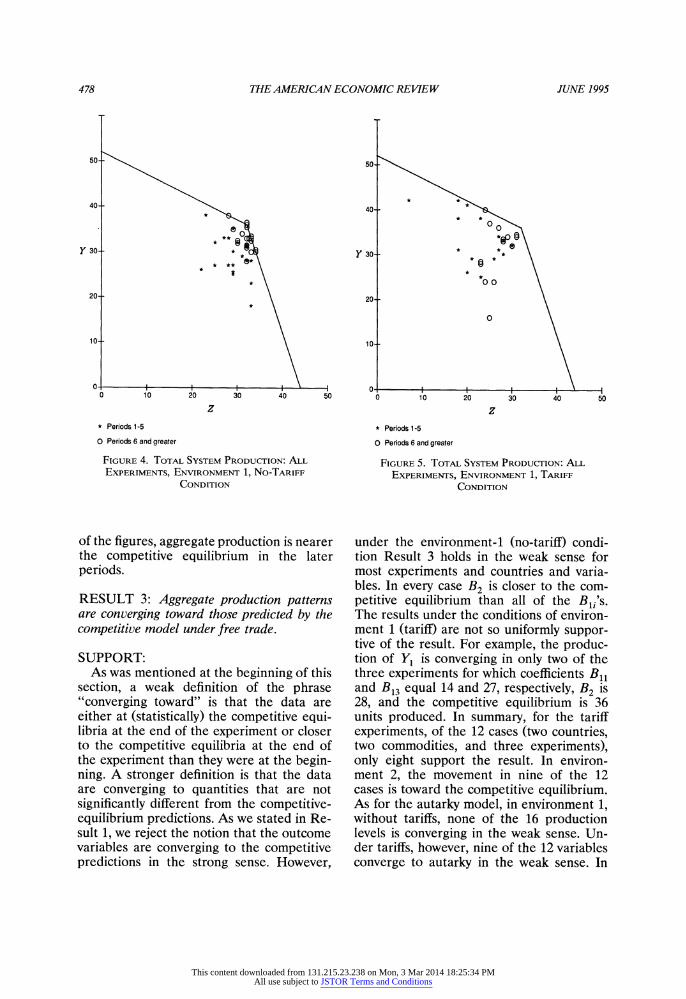
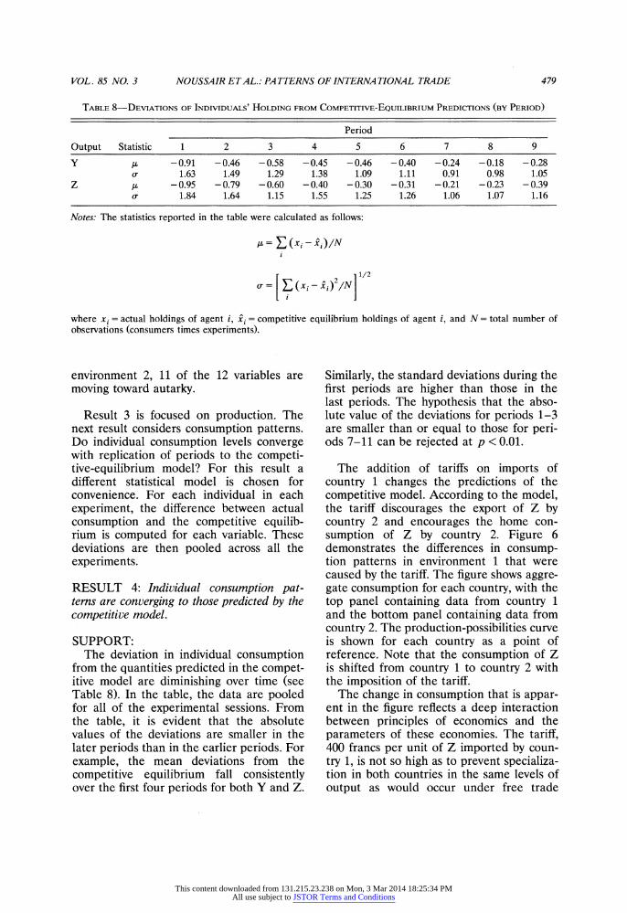
The support for Result 3 can be seen in Figures 4 and 5 for environment 1. The figures contain world aggregate production for early periods and for later periods. The world production frontier is shown in the figure. The competitive model predicts that world production will be at the "kink" in the frontier. Figure 4 contains data from environment-1 experiments in which there were no tariffs. Figure 5 contains the data from environment-1 experiments in which tariffs existed. As can be seen in both
This content downloaded from 131.215.23.238 on Mon, 3 Mar 2014 18:25:34 PMAll use subject to JSTOR Terms and Conditions
478 THE AMERICAN ECONOMIC REWEVW JUNE 1995
50-
40-\
.~~~~~~~ **a Y 30- * *
* * \*
20-*
10C-
0- 0 10 20 30 40 50
z
* Periods 1-5
o Periods 6 and greater
FIGURE 4. TOTAL SYSTEM PRODUCTION: ALL
EXPERIMENTS, ENVIRONMENT 1, NO-TARIFF
CONDITION
of the figures, aggregate production is nearer the competitive equilibrium in the later periods.
RESULT 3: Aggregate production patterns are conuerging toward those predicted by the competitive model under free trade.
SUPPORT: As was mentioned at the beginning of this
section, a weak definition of the phrase ''converging toward" is that the data are either at (statistically) the competitive equi- libria at the end of the experiment or closer to the competitive equilibria at the end of the experiment than they were at the begin- ning. A stronger definition is that the data are converging to quantities that are not significantly different from the competitive- equilibrium predictions. As we stated in Re- sult 1, we reject the notion that the outcome variables are converging to the competitive predictions in the strong sense. However,
50
40- *
00
Y 30- *
00
20-\
0
10-
0 0 10 20 30 40 50
z
* Periods 1-5
0 Perods 6 and greater
FIGURE 5. TOTAL SYSTEM PRODUCTION: ALL
EXPERIMENTS, ENVIRONMENT 1, TARIFF
CONDITION
under the environment-1 (no-tariff) condi- tion Result 3 holds in the weak sense for most experiments and countries and varia- bles. In every case B2 is closer to the com- petitive equilibrium than all of the B1 's. The results under the conditions of environ- ment 1 (tariff) are not so uniformly suppor- tive of the result. For example, the produc- tion of Y1 is converging in only two of the three experiments for which coefficients B11 and B13 equal 14 and 27, respectively, B2 is 28, and the competitive equilibrium is 36 units produced. In summary, for the tariff experiments, of the 12 cases (two countries, two commodities, and three experiments), only eight support the result. In environ- ment 2, the movement in nine of the 12 cases is toward the competitive equilibrium. As for the autarky model, in environment 1, without tariffs, none of the 16 production levels is converging in the weak sense. Un- der tariffs, however, nine of the 12 variables converge to autarky in the weak sense. In
This content downloaded from 131.215.23.238 on Mon, 3 Mar 2014 18:25:34 PMAll use subject to JSTOR Terms and Conditions
VOL. 85 NO. 3 NOUSSAIR ETAL.: PATTERNS OF INTERNATIONAL TRADE 479
TABLE 8-DEVIATIONS OF INDIVIDUALS' HOLDING FROM COMPETITIVE-EQUILIBRIUM PREDICTIONS (BY PERIOD)
Period
Output Statistic 1 2 3 4 5 6 7 8 9
Y ,U -0.91 -0.46 -0.58 -0.45 -0.46 -0.40 -0.24 -0.18 -0.28 Cr 1.63 1.49 1.29 1.38 1.09 1.11 0.91 0.98 1.05
Z -0.95 - 0.79 -0.60 -0.40 - 0.30 -0.31 -0.21 -0.23 - 0.39 1.84 1.64 1.15 1.55 1.25 1.26 1.06 1.07 1.16
Notes: The statistics reported in the table were calculated as follows:
" L(Xi- xi)/
where xi = actual holdings of agent i, ?i = competitive equilibrium holdings of agent i, and N = total number of observations (consumers times experiments).
environment 2, 11 of the 12 variables are moving toward autarky.
Result 3 is focused on production. The next result considers consumption patterns. Do individual consumption levels converge with replication of periods to the competi- tive-equilibrium model? For this result a different statistical model is chosen for convenience. For each individual in each experiment, the difference between actual consumption and the competitive equilib- rium is computed for each variable. These deviations are then pooled across all the experiments.
RESULT 4: Individual consumption pat- terns are converging to those predicted by the competitive model.
SUPPORT: The deviation in individual consumption
from the quantities predicted in the compet- itive model are diminishing over time (see Table 8). In the table, the data are pooled for all of the experimental sessions. From the table, it is evident that the absolute values of the deviations are smaller in the later periods than in the earlier periods. For example, the mean deviations from the competitive equilibrium fall consistently over the first four periods for both Y and Z.
Similarly, the standard deviations during the first periods are higher than those in the last periods. The hypothesis that the abso- lute value of the deviations for periods 1-3 are smaller than or equal to those for peri- ods 7-11 can be rejected at p < 0.01.
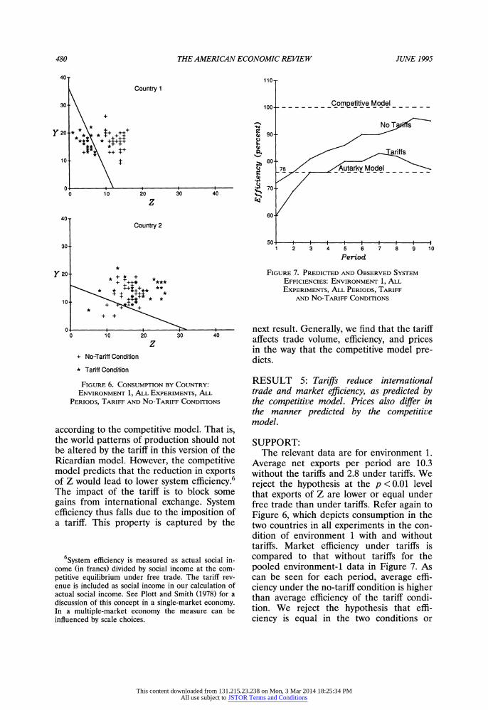
The addition of tariffs on imports of country 1 changes the predictions of the competitive model. According to the model, the tariff discourages the export of Z by country 2 and encourages the home con- sumption of Z by country 2. Figure 6 demonstrates the differences in consump- tion patterns in environment 1 that were caused by the tariff. The figure shows aggre- gate consumption for each country, with the top panel containing data from country 1 and the bottom panel containing data from country 2. The production-possibilities curve is shown for each country as a point of reference. Note that the consumption of Z is shifted from country 1 to country 2 with the imposition of the tariff.
The change in consumption that is appar- ent in the figure reflects a deep interaction between principles of economics and the parameters of these economies. The tariff, 400 francs per unit of Z imported by coun- try 1, is not so high as to prevent specializa- tion in both countries in the same levels of output as would occur under free trade
This content downloaded from 131.215.23.238 on Mon, 3 Mar 2014 18:25:34 PMAll use subject to JSTOR Terms and Conditions
480 THE AMERICAN ECONOMIC REoVIEW JUNE 1995
40- .
Country 1
30
y 20-.* ++ ounry
+
+:++
10 4:
0 10 20 30 40
z 40T
Country 2
30-
_1- *
1 0 * ++ t+ * ***
0 0 10 20 30 40
z
+ No-Tariff Condition
* Tariff Condition
FIGURE 6. CONSUMPTION BY COUNTRY:
ENVIRONMENT 1, ALL EXPERIMENTS, ALL
PERIODS, TARIFF AND NO-TARIFF CONDITIONS
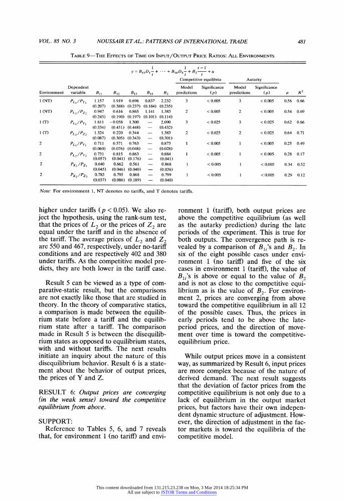
according to the competitive model. That is, the world patterns of production should not be altered by the tariff in this version of the Ricardian model. However, the competitive model predicts that the reduction in exports of Z would lead to lower system efficiency.6 The impact of the tariff is to block some gains from international exchange. System efficiency thus falls due to the imposition of a tariff. This property is captured by the
110-
100 .. . . . . . ..Corpetitive Model
NoT- @ 90-.
ariffs 80-7
76 Autarky Model
70
60
50 l l I l l l l I 1 2 3 4 5 6 7 8 9 10
Period
FIGURE 7. PREDICTED AND OBSERVED SYSTEM
EFFICIENCIES: ENVIRONMENT 1, ALL
EXPERIMENTS, ALL PERIODS, TARIFF
AND NO-TARIFF CONDITIONS
next result. Generally, we find that the tariff affects trade volume, efficiency, and prices in the way that the competitive model pre- dicts.
RESULT 5: Tariffs reduce international trade and market efficiency, as predicted by the competitive model. Prices also differ in the manner predicted by the competitive model.
SUPPORT: The relevant data are for environment 1.
Average net exports per period are 10.3 without the tariffs and 2.8 under tariffs. We reject the hypothesis at the p <0.01 level that exports of Z are lower or equal under free trade than under tariffs. Refer again to Figure 6, which depicts consumption in the two countries in all experiments in the con- dition of environment 1 with and without tariffs. Market efficiency under tariffs is compared to that without tariffs for the pooled environment-1 data in Figure 7. As can be seen for each period, average effi- ciency under the no-tariff condition is higher than average efficiency of the tariff condi- tion. We reject the hypothesis that effi- ciency is equal in the two conditions or
6System efficiency is measured as actual social in- come (in francs) divided by social income at the com- petitive equilibrium under free trade. The tariff rev- enue is included as social income in our calculation of actual social income. See Plott and Smith (1978) for a discussion of this concept in a single-market economy. In a multiple-market economy the measure can be influenced by scale choices.
This content downloaded from 131.215.23.238 on Mon, 3 Mar 2014 18:25:34 PMAll use subject to JSTOR Terms and Conditions
VOL. 85 NO. 3 NOUSSAIR ETAL.: PATTERNS OF INTERNATIONAL TRADE 481
TABLE 9-THE EFFECTS OF TIME ON INPUT/OUTPUT PRICE RATIOS: ALL ENVIRONMENTS
1 1 t-1 Y=BIIDI-+ *--+B14D4-+B2 +u
t t t
Competitive equilibria Autarky
Dependent Model Significance Model Significance Environment variable B11 B12 B13 B14 B2 predictions (p) predictions (p) p R2
1 (NT) PLJ/PYJ 1.157 1.919 0.696 0.837 2.232 3 < 0.005 3 < 0.005 0.56 0.66 (0.207) (0.388) (0.237) (0.184) (0.235)
1 (NT) PL2/PZ2 0.947 0.616 0.865 1.141 1.383 2 < 0.005 2 < 0.005 0.54 0.69 (0.243) (0.190) (0.197) (0.101) (0.114)
1(T) PL /PY, 1.611 -0.058 1.300 - 2.090 3 < 0.025 3 < 0.025 0.62 0.66 (0.334) (0.451) (0.448) - (0.432)
1(T) PL2/PZ2 1.324 0.220 0.344 - 1.383 2 < 0.025 2 < 0.025 0.64 0.71 (0.087) (0.305) (0.343) - (0.301)
2 PL /Py, 0.711 0.571 0.763 - 0.873 1 < 0.005 1 < 0.005 0.25 0.49 (0.060) (0.076) (0.048) - (0.028)
2 PL2/PY2 0.731 0.815 0.863 - 0.884 1 < 0.005 1 < 0.005 0.28 0.17 (0.057) (0.041) (0.176) - (0.041)
2 PK1 /PZ1 0.640 0.662 0.561 - 0.868 1 < 0.005 1 < 0.005 0.34 0.52 (0.045) (0.046) (0.040) - (0.036)
2 PK2/PZ2 0.783 0.795 0.868 - 0.799 1 < 0.005 1 < 0.005 0.29 0.12 (0.037) (0.086) (0.189) - (0.040)
Note: For environment 1, NT denotes no tariffs, and T denotes tariffs.
higher under tariffs (p < 0.05). We also re- ject the hypothesis, using the rank-sum test, that the prices of L2 or the prices of Z2 are equal under the tariff and in the absence of the tariff. The average prices of L2 and Z2 are 550 and 467, respectively, under no-tariff conditions and are respectively 402 and 380 under tariffs. As the competitive model pre- dicts, they are both lower in the tariff case.
Result 5 can be viewed as a type of com- parative-static result, but the comparisons are not exactly like those that are studied in theory. In the theory of comparative statics, a comparison is made between the equilib- rium state before a tariff and the equilib- rium state after a tariff. The comparison made in Result 5 is between the disequilib- rium states as opposed to equilibrium states, with and without tariffs. The next results initiate an inquiry about the nature of this disequilibrium behavior. Result 6 is a state- ment about the behavior of output prices, the prices of Y and Z.
RESULT 6: Output prices are converging (in the weak sense) toward the competitive equilibrium from above.
SUPPORT: Reference to Tables 5, 6, and 7 reveals
that, for environment 1 (no tariff) and envi-
ronment 1 (tariff), both output prices are above the competitive equilibrium (as well as the autarky prediction) during the late periods of the experiment. This is true for both outputs. The convergence path is re- vealed by a comparison of Bli's and B2. In six of the eight possible cases under envi- ronment 1 (no tariff) and five of the six cases in environment 1 (tariff), the value of B1 's is above or equal to the value of B2 and is not as close to the competitive equi- librium as is the value of B2. For environ- ment 2, prices are converging from above toward the competitive equilibrium in all 12 of the possible cases. Thus, the prices in early periods tend to be above the late- period prices, and the direction of move- ment over time is toward the competitive- equilibrium price.
While output prices move in a consistent way, as summarized by Result 6, input prices are more complex because of the nature of derived demand. The next result suggests that the deviation of factor prices from the competitive equilibrium is not only due to a lack of equilibrium in the output market prices, but factors have their own indepen- dent dynamic structure of adjustment. How- ever, the direction of adjustment in the fac- tor markets is toward the equilibria of the competitive model.
This content downloaded from 131.215.23.238 on Mon, 3 Mar 2014 18:25:34 PMAll use subject to JSTOR Terms and Conditions
482 THE AMERICAN ECONOMIC REVIEW JUNE 1995
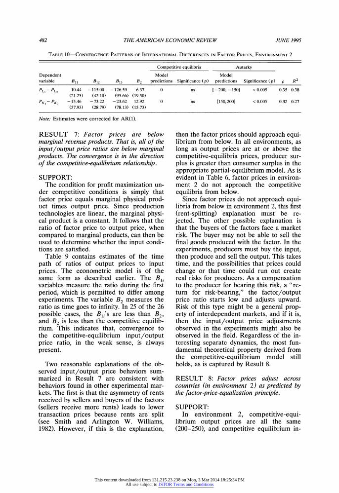
TABLE 10-CONVERGENCE PATTrERNS OF INTERNATIONAL DIFFERENCES IN FACTOR PRICES, ENVIRONMENT 2
Competitive equilibria Autarky
Dependent Model Model variable B1l B12 B13 B2 predictions Significance (p) predictions Significance (p) p R2
PL1 PL2 10.44 -115.00 - 126.59 6.37 0 ns [-200, -1501 < 0.005 0.35 0.38 (21.23) (42.10) (95.66) (19.50)
PK1 PK2 -15.46 - 73.22 -23.62 12.92 0 ns [150,2001 < 0.005 0.32 0.27 (37.93) (28.79) (78.13) (15.73)
Note: Estimates were corrected for AR(1).
RESULT 7: Factor prices are below marginal revenue products. That is, all of the input/output price ratios are below marginal products. The convergence is in the direction of the competitive-equilibrium relationship.
SUPPORT: The condition for profit maximization un-
der competitive conditions is simply that factor price equals marginal physical prod- uct times output price. Since production technologies are linear, the marginal physi- cal product is a constant. It follows that the ratio of factor price to output price, when compared to marginal products, can then be used to determine whether the input condi- tions are satisfied.
Table 9 contains estimates of the time path of ratios of output prices to input prices. The econometric model is of the same form as described earlier. The Bl1 variables measure the ratio during the first period, which is permitted to differ among experiments. The variable B2 measures the ratio as time goes to infinity. In 25 of the 26 possible cases, the B1i's are less than B2, and B2 is less than the competitive equilib- rium. This indicates that, convergence to the competitive-equilibrium input/output price ratio, in the weak sense, is always present.
Two reasonable explanations of the ob- served input/output price behaviors sum- marized in Result 7 are consistent with behaviors found in other experimental mar- kets. The first is that the asymmetry of rents received by sellers and buyers of the factors (sellers receive more rents) leads to lower transaction prices because rents are split (see Smith and Arlington W. Williams, 1982). However, if this is the explanation,
then the factor prices should approach equi- librium from below. In all environments, as long as output prices are at or above the competitive-equilibria prices, producer sur- plus is greater than consumer surplus in the appropriate partial-equilibrium model. As is evident in Table 6, factor prices in environ- ment 2 do not approach the competitive equilibria from below.
Since factor prices do not approach equi- libria from below in environment 2, this first (rent-splitting) explanation must be re- jected. The other possible explanation is that the buyers of the factors face a market risk. The buyer may not be able to sell the final goods produced with the factor. In the experiments, producers must buy the input, then produce and sell the output. This takes time, and the possibilities that prices could change or that time could run out create real risks for producers. As a compensation to the producer for bearing this risk, a "re- turn for risk-bearing," the factor/output price ratio starts low and adjusts upward. Risk of this type might be a general prop- erty of interdependent markets, and if it is, then the input/output price adjustments observed in the experiments might also be observed in the field. Regardless of the in- teresting separate dynamics, the most fun- damental theoretical property derived from the competitive-equilibrium model still holds, as is captured by Result 8.
RESULT 8: Factor prices adjust across countries (in environment 2) as predicted by the factor-price-equalization principle.
SUPPORT: In environment 2, competitive-equi-
librium output prices are all the same (200-250), and competitive equilibrium in-
This content downloaded from 131.215.23.238 on Mon, 3 Mar 2014 18:25:34 PMAll use subject to JSTOR Terms and Conditions
VOL. 85 NO. 3 NOUSSAIR ETAL.: PATTERNS OF INTERNATIONAL TRADE 483
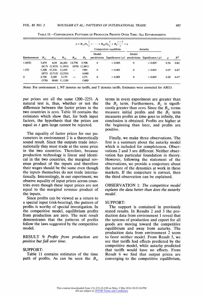
TABLE 11-CONVERGENCE PATrERNS OF PRODUCER PROFITS OVER TIME: ALL ENVIRONMENTS
1 1 t-1 y=B11D1- + +B14D4-+B2 +u
t t t Competitive equilibria Autarky
Model Model
Environment B1l B12 B13 B14 B2 predictions Significance (p) predictions Significance (p) p R2
1 (NT) 7,479 6,93 24,200 13,778 5,798 0 < 0.005 0 < 0.005 0.54 0.82
(817) (2,953) (1,935) (879) (1,381) 1 (T) 5,300 35,336 12,699 - 1985 0 <0.005 0 <0.005 0.07 0.87
(875) (3,713) (2,550) (648) 2 3,730 3,085 3,179 - 1271 0 < 0.005 0 < 0.005 0.20 0.47
(378) (868) (1,128) (188)
Notes: For environment 1, NT denotes no tariffs, and T denotes tariffs. Estimates were corrected for AR(1).
put prices are all the same (200-225). A natural test is, thus, whether or not the difference between the factor prices in the two countries is zero. Table 10 contains the estimates which show that, for both input factors, the hypothesis that the prices are equal as t gets large cannot be rejected.
The equality of factor prices for our pa- rameters in environment 2 is a theoretically sound result. Since the outputs trade inter- nationally they must trade at the same price in the two countries. Therefore, because production technology is linear and identi- cal in the two countries, the marginal rev- enue product of the inputs and therefore their wages should be the same even though the inputs themselves do not trade interna- tionally. Interestingly, in our experiment, we observe equality of input prices across coun- tries even though these input prices are not equal to the marginal revenue product of the inputs.
Since profits can be viewed as a return to a special input (risk-bearing), the pattern of profits is worthy of special investigation. In the competitive model, equilibrium profits from production are zero. The next result demonstrates that the patterns of profits follow the laws suggested by the competitive model.
RESULT 9: Profits from production are positive but fall over time.
SUPPORT: Table 11 contains estimates of the time
path of profits. As can be seen the Bli
terms in every experiment are greater than the B2 term. Furthermore, B2 is signifi- cantly greater than zero. Since the B1i terms measure initial profits and the B2 term measures profits as time goes to infinity, the conclusion is obtained. Profits are higher at the beginning than later, and profits are positive.
Finally, we make three observations. The first is a summary about the autarky model which is included for completeness. Obser- vations 2 and 3 are different. Neither obser- vation has particular foundation in theory. However, following the statement of the observations, we provide a conjecture about the nature of the dynamics at work in these markets. If the conjecture is correct, then the third observation can be explained.
OBSERVATION 1: The competitive model explains the data better than does the autarky model.
SUPPORT: The support is contained in previously
stated results. In Results 2 and 3 the pro- duction data from environment 1 reveal that the systems of production and export for all goods are moving toward the competitive equilibrium and away from autarky. The production data from environment 2 seem to favor neither model. From Result 5, we see that tariffs had effects predicted by the competitive model, while autarky predicted that tariffs would have no effects. From Result 6 we find that output prices are converging to the competitive equilibrium,
This content downloaded from 131.215.23.238 on Mon, 3 Mar 2014 18:25:34 PMAll use subject to JSTOR Terms and Conditions
484 THE AMERICAN ECONOMIC REVIEW JUNE 1995
60-
50-
40-
Y 30--
20-\
10_
0 0 10 20 30 40 50
z
O No Tariff Condition
* Tariff condition
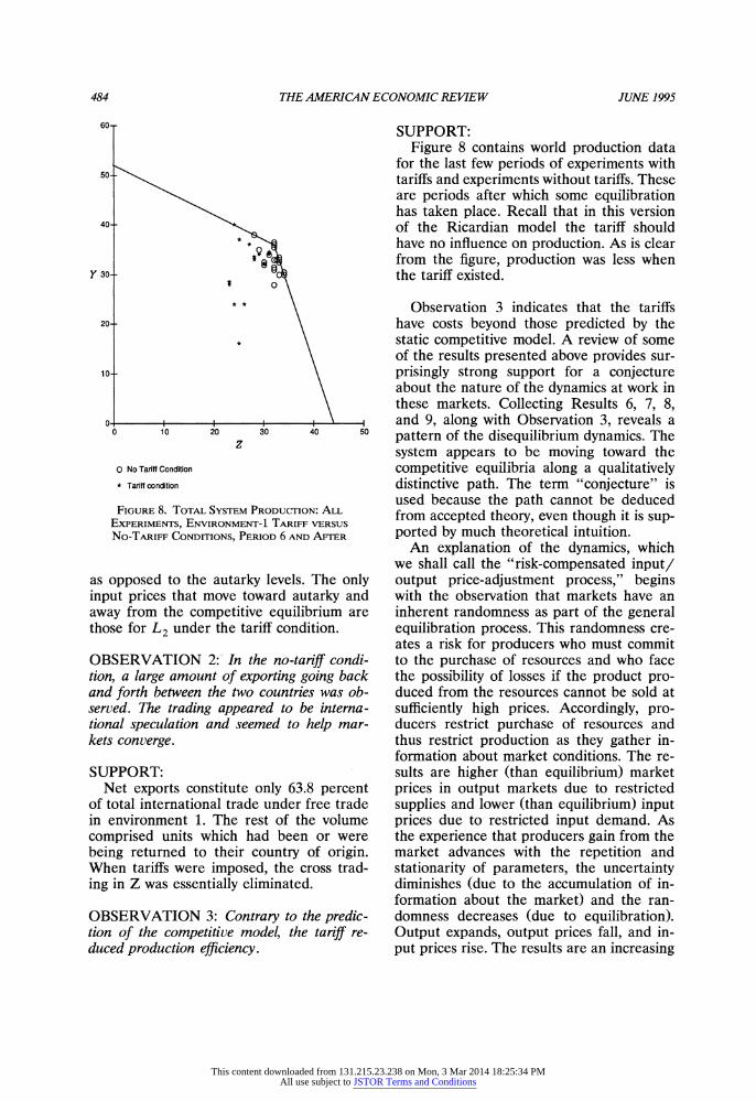
FIGURE 8. TOTAL SYSTEM PRODUCTION: ALL EXPERIMENTS, ENVIRONMENT-1 TARIFF VERSUS
NO-TARIFF CONDITIONS, PERIOD 6 AND AFFTER
as opposed to the autarky levels. The only input prices that move toward autarky and away from the competitive equilibrium are those for L2 under the tariff condition.
OBSERVATION 2: In the no-tarif condi- tion, a large amount of exporting going back and forth between the two countries was ob- served. The trading appeared to be intemaa- tional speculation and seemed to help mar- kets converge.
SUPPORT: Net exports constitute only 63.8 percent
of total international trade under free trade in environment 1. The rest of the volume comprised units which had been or were being returned to their country of origin. When tariffs were imposed, the cross trad- ing in Z was essentially eliminated.
OBSERVATION 3: Contrary to the predic- tion of the competitive model, the tariff re- duced production efficiency.
SUPPORT: Figure 8 contains world production data
for the last few periods of experiments with tariffs and experiments without tariffs. These are periods after which some equilibration has taken place. Recall that in this version of the Ricardian model the tariff should have no influence on production. As is clear from the figure, production was less when the tariff existed.
Observation 3 indicates that the tariffs have costs beyond those predicted by the static competitive model. A review of some of the results presented above provides sur- prisingly strong support for a conjecture about the nature of the dynamics at work in these markets. Collecting Results 6, 7, 8, and 9, along with Observation 3, reveals a pattern of the disequilibrium dynamics. The system appears to be moving toward the competitive equilibria along a qualitatively distinctive path. The term "conjecture" is used because the path cannot be deduced from accepted theory, even though it is sup- ported by much theoretical intuition.
An explanation of the dynamics, which we shall call the "risk-compensated input/ output price-adjustment process," begins with the observation that markets have an inherent randomness as part of the general equilibration process. This randomness cre- ates a risk for producers who must commit to the purchase of resources and who face the possibility of losses if the product pro- duced from the resources cannot be sold at sufficiently high prices. Accordingly, pro- ducers restrict purchase of resources and thus restrict production as they gather in- formation about market conditions. The re- sults are higher (than equilibrium) market prices in output markets due to restricted supplies and lower (than equilibrium) input prices due to restricted input demand. As the experience that producers gain from the market advances with the repetition and stationarity of parameters, the uncertainty diminishes (due to the accumulation of in- formation about the market) and the ran- domness decreases (due to equilibration). Output expands, output prices fall, and in- put prices rise. The results are an increasing
This content downloaded from 131.215.23.238 on Mon, 3 Mar 2014 18:25:34 PMAll use subject to JSTOR Terms and Conditions
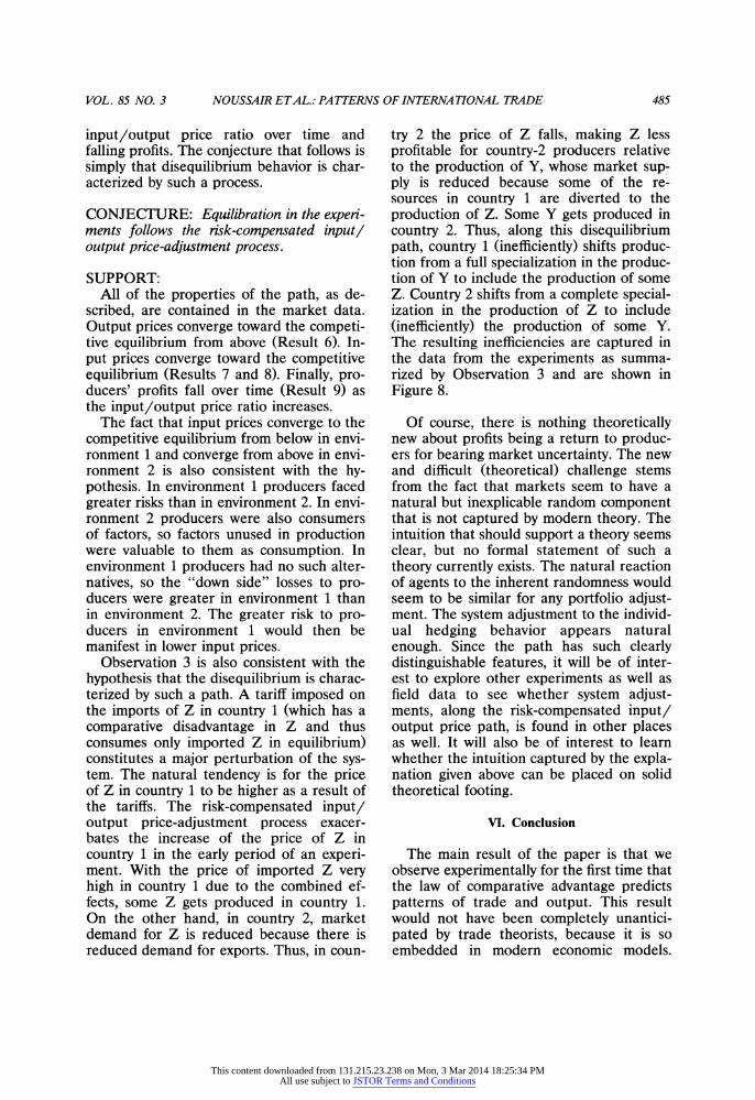
VOL. 85 NO. 3 NOUSSAIR ETAL.: PATTERNS OF INTERNATIONAL TRADE 485
input/output price ratio over time and falling profits. The conjecture that follows is simply that disequilibrium behavior is char- acterized by such a process.
CONJECTURE: Equilibration in the experi- ments follows the risk-compensated input/ output price-adjustment process.
SUPPORT: All of the properties of the path, as de-
scribed, are contained in the market data. Output prices converge toward the competi- tive equilibrium from above (Result 6). In- put prices converge toward the competitive equilibrium (Results 7 and 8). Finally, pro- ducers' profits fall over time (Result 9) as the input/output price ratio increases.
The fact that input prices converge to the competitive equilibrium from below in envi- ronment 1 and converge from above in envi- ronment 2 is also consistent with the hy- pothesis. In environment 1 producers faced greater risks than in environment 2. In envi- ronment 2 producers were also consumers of factors, so factors unused in production were valuable to them as consumption. In environment 1 producers had no such alter- natives, so the "down side" losses to pro- ducers were greater in environment 1 than in environment 2. The greater risk to pro- ducers in environment 1 would then be manifest in lower input prices.
Observation 3 is also consistent with the hypothesis that the disequilibrium is charac- terized by such a path. A tariff imposed on the imports of Z in country 1 (which has a comparative disadvantage in Z and thus consumes only imported Z in equilibrium) constitutes a major perturbation of the sys- tem. The natural tendency is for the price of Z in country 1 to be higher as a result of the tariffs. The risk-compensated input/ output price-adjustment process exacer- bates the increase of the price of Z in country 1 in the early period of an experi- ment. With the price of imported Z very high in country 1 due to the combined ef- fects, some Z gets produced in country 1. On the other hand, in country 2, market demand for Z is reduced because there is reduced demand for exports. Thus, in coun-
try 2 the price of Z falls, making Z less profitable for country-2 producers relative to the production of Y, whose market sup- ply is reduced because some of the re- sources in country 1 are diverted to the production of Z. Some Y gets produced in country 2. Thus, along this disequilibrium path, country 1 (inefficiently) shifts produc- tion from a full specialization in the produc- tion of Y to include the production of some Z. Country 2 shifts from a complete special- ization in the production of Z to include (inefficiently) the production of some Y. The resulting inefficiencies are captured in the data from the experiments as summa- rized by Observation 3 and are shown in Figure 8.
Of course, there is nothing theoretically new about profits being a return to produc- ers for bearing market uncertainty. The new and difficult (theoretical) challenge stems from the fact that markets seem to have a natural but inexplicable random component that is not captured by modern theory. The intuition that should support a theory seems clear, but no formal statement of such a theory currently exists. The natural reaction of agents to the inherent randomness would seem to be similar for any portfolio adjust- ment. The system adjustment to the individ- ual hedging behavior appears natural enough. Since the path has such clearly distinguishable features, it will be of inter- est to explore other experiments as well as field data to see whether system adjust- ments, along the risk-compensated input/ output price path, is found in other places as well. It will also be of interest to learn whether the intuition captured by the expla- nation given above can be placed on solid theoretical footing.
VI. Conclusion
The main result of the paper is that we observe experimentally for the first time that the law of comparative advantage predicts patterns of trade and output. This result would not have been completely unantici- pated by trade theorists, because it is so embedded in modern economic models.
This content downloaded from 131.215.23.238 on Mon, 3 Mar 2014 18:25:34 PMAll use subject to JSTOR Terms and Conditions
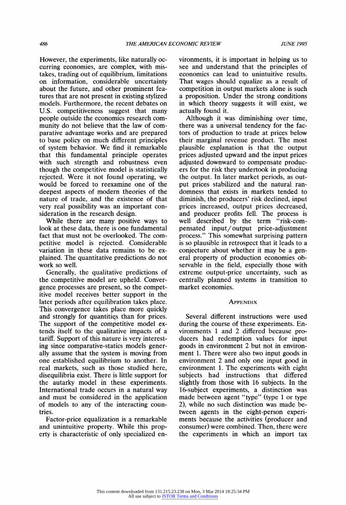
486 THE AMERICAN ECONOMIC REVIEW JUNE 1995
However, the experiments, like naturally oc- curring economies, are complex, with mis- takes, trading out of equilibrium, limitations on information, considerable uncertainty about the future, and other prominent fea- tures that are not present in existing stylized models. Furthermore, the recent debates on U.S. competitiveness suggest that many people outside the economics research com- munity do not believe that the law of com- parative advantage works and are prepared to base policy on much different principles of system behavior. We find it remarkable that this fundamental principle operates with such strength and robustness even though the competitive model is statistically rejected. Were it not found operating, we would be forced to reexamine one of the deepest aspects of modern theories of the nature of trade, and the existence of that very real possibility was an important con- sideration in the research design.
While there are many positive ways to look at these data, there is one fundamental fact that must not be overlooked. The com- petitive model is rejected. Considerable variation in these data remains to be ex- plained. The quantitative predictions do not work so well.
Generally, the qualitative predictions of the competitive model are upheld. Conver- gence processes are present, so the compet- itive model receives better support in the later periods after equilibration takes place. This convergence takes place more quickly and strongly for quantitiqs than for prices. The support of the competitive model ex- tends itself to the qualitative impacts of a tariff. Support of this nature is very interest- ing since comparative-statics models gener- ally assume that the system is moving from one established equilibrium to another. In real markets, such as those studied here, disequilibria exist. There is little support for the autarky model in these experiments. International trade occurs in a natural way and must be considered in the application of models to any of the interacting coun- tries.
Factor-price equalization is a remarkable and unintuitive property. While this prop- erty is characteristic of only specialized en-
vironments, it is important in helping us to see and understand that the principles of economics can lead to unintuitive results. That wages should equalize as a result of competition in output markets alone is such a proposition. Under the strong conditions in which theory suggests it will exist, we actually found it.
Although it was diminishing over time, there was a universal tendency for the fac- tors of production to trade at prices below their marginal revenue product. The most plausible explanation is that the output prices adjusted upward and the input prices adjusted downward to compensate produc- ers for the risk they undertook in producing the output. In later market periods, as out- put prices stabilized and the natural ran- domness that exists in markets tended to diminish, the producers' risk declined, input prices increased, output prices decreased, and producer profits fell. The process is well described by the term "risk-com- pensated input/ output price-adjustment process." This somewhat surprising pattern is so plausible in retrospect that it leads to a conjecture about whether it may be a gen- eral property of production economies ob- servable in the field, especially those with extreme output-price uncertainty, such as centrally planned systems in transition to market economies.
APPENDIX
Several different instructions were used during the course of these experiments. En- vironments 1 and 2 differed because pro- ducers had redemption values for input goods in environment 2 but not in environ- ment 1. There were also two input goods in environment 2 and only one input good in environment 1. The experiments with eight subjects had instructions that differed slightly from those with 16 subjects. In the 16-subject experiments, a distinction was made between agent "type" (type 1 or type 2), while no such distinction was made be- tween agents in the eight-person experi- ments because the activities (producer and consumer) were combined. Then, there were the experiments in which an import tax
This content downloaded from 131.215.23.238 on Mon, 3 Mar 2014 18:25:34 PMAll use subject to JSTOR Terms and Conditions
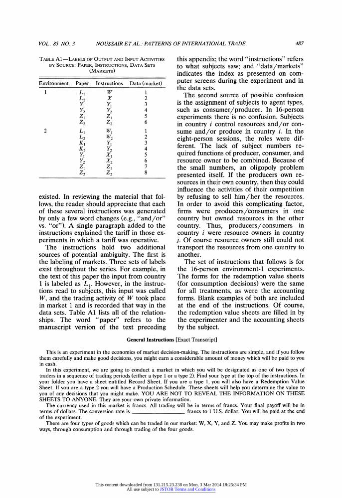
VOL. 85 NO. 3 NOUSSAIR ETAL.: PATTERNS OF INTERNATIONAL TRADE 487
TABLE Al -LABELS OF OUTPUT AND INPUT AcTIVITIES
BY SOURCE: PAPER, INSTRUCTIONS, DATA SETS
(MARKETS)
Environment Paper Instructions Data (market)
1 L W v 1 L2 X 2 Y, Y, 3 Y2 Y2 4 Z1 Z5 S Z2 Z2 6
2 L, WI 1 L2 W2 2 K, Y, 3 K2 Y2 4 Y, Xl S
Y2 X2 6 Z, Z, 7 Z2 Z2 8
existed. In reviewing the material that fol- lows, the reader should appreciate that each of these several instructions was generated by only a few word changes (e.g., "'and/or"' vs. "or"). A single paragraph added to the instructions explained the tariff in those ex- periments in which a tariff was operative.
The instructions hold two additional sources of potential ambiguity. The first is the labeling of markets. Three sets of labels exist throughout the series. For example, in the text of this paper the input from country 1 is labeled as L . However, in the instruc- tions read to subjects, this input was called W, and the trading activity of W took place in market 1 and is recorded that way in the data sets. Table Al lists all of the relation- ships. The word "paper" refers to the manuscript version of the text preceding
this appendix; the word "instructions" refers to what subjects saw; and "data/markets" indicates the index as presented on com- puter screens during the experiment and in the data sets.
The second source of possible confusion is the assignment of subjects to agent types, such as consumer/producer. In 16-person experiments there is no confusion. Subjects in country i control resources and/or con- sume and/or produce in country i. In the eight-person sessions, the roles were dif- ferent. The lack of subject numbers re- quired functions of producer, consumer, and resource owner to be combined. Because of the small numbers, an oligopoly problem presented itself. If the producers own re- sources in their own country, then they could influence the activities of their competition by refusing to sell him/her the resources. In order to avoid this complicating factor, firms were producers/consumers in one country but owned resources in the other country. Thus, producers/consumers in country i were resource owners in country j. Of course resource owners still could not transport the resources from one country to another.
The set of instructions that follows is for the 16-person environment-1 experiments. The forms for the redemption value sheets (for consumption decisions) were the same for all treatments, as were the accounting forms. Blank examples of both are included at the end of the instructions. Of course, the redemption value sheets are filled in by the experimenter and the accounting sheets by the subject.
General Instructions [Exact Transcript]
This is an experiment in the economics of market decision-making. The instructions are simple, and if you follow them carefully and make good decisions, you might earn a considerable amount of money which will be paid to you in cash.
In this experiment, we are going to conduct a market in which you will be designated as one of two types of traders in a sequence of trading periods (either a type 1 or a type 2). Find your type at the top of the instructions. In your folder you have a sheet entitled Record Sheet. If you are a type 1, you will also have a Redemption Value Sheet. If you are a type 2 you will have a Production Schedule. These sheets will help you determine the value to you of any decisions that you might make. YOU ARE NOT TO REVEAL THE INFORMATION ON THESE SHEETS TO ANYONE. They are your own private information.
The currency used in this market is francs. All trading will be in terms of francs. Your final payoff will be in terms of dollars. The conversion rate is francs to 1 U.S. dollar. You will be paid at the end of the experiment.
There are four types of goods which can be traded in our market: W, X, Y, and Z. You may make profits in two ways, through consumption and through trading of the four goods.
This content downloaded from 131.215.23.238 on Mon, 3 Mar 2014 18:25:34 PMAll use subject to JSTOR Terms and Conditions
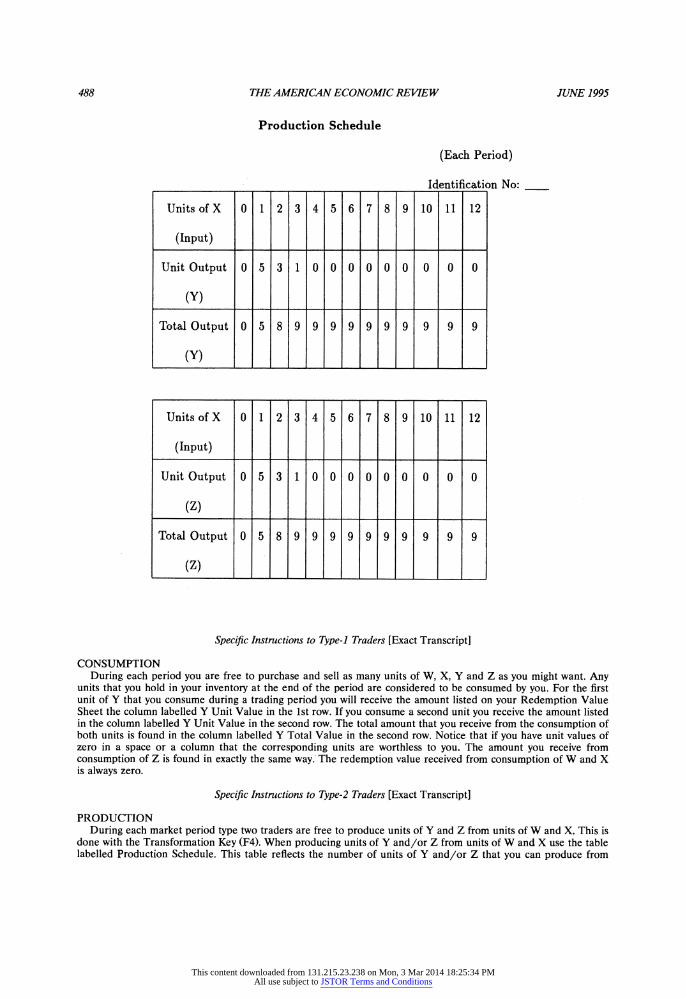
488 THE AMERICAN ECONOMIC REVIEW JUNE 1995
Production Schedule
(Each Period)
____________ Identification No:
Units of X 0 1 2 3 4 5 6 7 8 9 10 11 12
(Input)
Unit Output 0 5 3 1 0 0 0 0 00 0 0 0
(Y)
Total Output 0 5 8 9 9 9 9 9 9 9 9 9 9
(Y)
Units of X 0 1 2 3 4 5 6 7 8 9 10 11 12
(Input)
Unit Output 0 5 3 1 0 0 0 000 0 0 0
(Z)
Total Output 0 5 8 9 9 9 9 9 9 9 9 9 9
(Z)
Specific Instructions to Type-i Traders [Exact Transcript]
CONSUMPTION During each period you are free to purchase and sell as many units of W, X, Y and Z as you might want. Any
units that you hold in your inventory at the end of the period are considered to be consumed by you. For the first unit of Y that you consume during a trading period you will receive the amount listed on your Redemption Value Sheet the column labelled Y Unit Value in the 1st row. If you consume a second unit you receive the amount listed in the column labelled Y Unit Value in the second row. The total amount that you receive from the consumption of both units is found in the column labelled Y Total Value in the second row. Notice that if you have unit values of zero in a space or a column that the corresponding units are worthless to you. The amount you receive from consumption of Z is found in exactly the same way: The redemption value received from consumption of W and X is always zero.
Specific Instructions to Type-2 Traders [Exact Transcript]
PRODUCTION During each market period type two traders are free to produce units of Y and Z from units of W and X. This is
done with the Transformation Key (F4). When producing units of Y and/or Z from units of W and X use the table labelled Production Schedule. This table reflects the number of units of Y and/or Z that you can produce from
This content downloaded from 131.215.23.238 on Mon, 3 Mar 2014 18:25:34 PMAll use subject to JSTOR Terms and Conditions

VOL. 85 NO. 3 NOUSSAIR ETAL..: PATTERNS OF INTERNATIONAL TRADE 489
REDEMPTION VALUE SHEET
(For Consumption Decisions)
Unit W unit W total X unit X total Y unit Y total Z unit Z total
value value value value value value value value
2
3
4
5
6
7
8
given amounts of W and X for the whole period. You have already been instructed in how to read the production schedule, but the following hypothetical example may provide further clarification.
Example: Suppose that you have 2 units of X and you have the Production Schedule shown on the next page [previous page in this appendix]. You can produce either:
a) 8 units of Y b) 5 units of Y and 5 units of Z c) 8 units of Z
Instructions to Both Types [Exact Transcript]
TRADING PROFITS Another source of profits is from buying and selling the four types of goods. Selling increases your cash on hand
by the amount of the sale price. Buying reduces your cash on hand by the amount of the purchase. Thus you can either gain or lose money on the purchase and resale of units.
EARNINGS Your profits each period are computed by taking the redemption values of the units of W, X, Y, and Z that you
consumed that period, adding the total sale price of the units of that you sold during the period and then subtracting the total of the prices you paid for the units that you bought during the period. The profits that you make exactly equal the change in your cash on hand from the beginning to the end of the period plus the redemption values of the units you consume.
At the end of the period enter the total number of units that you consume of W, X, Y, and Z at the top of your Record Sheet. Then, fill out the rest of your record sheet as follows. In line 2, fill in your Cash on Hand at the beginning of the period. In line 1, fill in your cash on hand at the end of the period. In line 3 fill in line 1 minus line 2. In lines 4-7 fill in your earnings from the consumption of W, X, Y, and Z. In line 8 add the total of lines 4-7. In line 9 add the total of lines 3 and 8. This amount is equal to your profits for the period (in francs).
ENDOWMENTS 1) At the beginning of each period you will be given an endowment of either W or X. This endowment will
appear in your inventory and will remain the same every period. You are free to sell any part of this endowment to anyone who might want to buy it.
2) At the beginning of the experiment you will receive 100000 francs cash on hand.
This content downloaded from 131.215.23.238 on Mon, 3 Mar 2014 18:25:34 PMAll use subject to JSTOR Terms and Conditions
490 THE AMERICAN ECONOMIC REVIEW JUNE 1995
Record Sheet
Period = 1
W X Y =
(1) Cash on hand at end of period
(2) Cash on hand at beginning of period
(3) Net change in cash on hand (l)-(2)
Earnings from consumption
(4) W
(5) X
(6) Y
(7) Z
(8) Total earnings from consumption (4)+(5)+(6)+(7)
(9) TOTAL PROFITS FOR THE PERIOD
HOW THE SYSTEM WORKS Type 1 people are endowed with W or X but would like to consume Y and Z. They can sell W or X to type 2
people to increase their cash in order to buy Y and Z. Type 2 people are endowed with W or X but may purchase additional units from type 1 people. They can produce Y and Z from W or X and sell them to type 1 people to increase their cash.
MARKET RESTRICTIONS Some of you may not be able to trade in all markets. You may not trade in markets
Unless you are informed otherwise these markets will be closed to you for the entire experiment. You may be taxed for trading in market 6. The tax that you pay is francs for each unit
that you buy or sell in that market. Unless you are informed otherwise, the tax will remain the same for the entire experiment.
REFERENCES
Ashenfelter, Orley; Currie, Janet; Farber, Henry S. and Spiegel, Matthew. "An Experimental Comparison of Dispute Rates in Alterna- tive Arbitration Systems." Econometrica, November 1992, 60(6), pp. 1407-33.
Caves, Richard; Frenkel, J. and Jones, R. World trade and payments, 5th Ed. Glenview, IL: Scott Foresman/Little Brown, 1990.
Chipman, John S. "A Survey of the Theory of International Trade: Part I, the Classical Theory." Econometrica, July 1965, 33(3), pp. 477-511.
Deardorff, Alan. "Testing Trade Theories and
Predicting Trade Flows," in Ronald W. Jones and Peter Kenen, eds., Handbook of international economics. Amsterdam: North-Holland, 1984, pp. 467-517.
Goodfellow, Jessica and Plott, Charles R. "An Experimental Examination of the Simul- taneous Determination of Input Prices and Output Prices." Southern Economic Journal, April 1990, 56(4), pp. 969-83.
Gremmen, Hans. "Testing the Factor Price Equalization Theorem in the EC: An Al- ternative Approach." Journal of Common Market Studies, March 1985, 23(3), pp. 278-86.
Lian, Peng and Plott, Charles R. "General
This content downloaded from 131.215.23.238 on Mon, 3 Mar 2014 18:25:34 PMAll use subject to JSTOR Terms and Conditions
VOL. 85 NO. 3 NOUSSAIR ETAL.: PATTERNS OF INTERNATIONAL TRADE 491
Equilibrium, Macroeconomics, and Moneyin a Laboratory Experimental En- vironment." California Institute of Tech- nology Social Science Working Paper No. 842, March 1993.
MacDougall, G. D. A. "British and American Exports: A Study Suggested by the The- ory of Comparative Costs, Part I." Eco- nomic Journal, December 1951, 61(244), pp. 697-724. _ . "British and American Exports: A Study Suggested by the Theory of Comparative Costs, Part II." Economic Journal, September 1952, 62(247), pp. 487-521.
Mokhtari, Manouchehr and Rassekh, Farhad. "The Tendency Towards Factor Price Equalization Among OECD Countries." Review of Economics and Statistics, November 1989, 71(4), pp. 636-42.
Plott, Charles R. "A Computerized Labora- tory Market System and Research Sup- port Systems for the Multiple Unit
Double Auction." California Institute of Technology Social Science Working Paper No. 783, November 1991.
Plott, Charles R. and Smith, Vernon L. "An Experimental Examination of Two Ex- change Institutions." Review of Economic Studies, February 1978, 45(1), pp. 133-53.
Porter, Michael P. The competitive advantage of nations. New York: Free Press, 1990.
Smith, Vernon L. and Williams, Arlington W. "The Effects of Rent Asymmetries in Ex- perimental Auction Markets." Journal of Economic Behavior and Organization, March 1982, 3(1), pp. 99-116.
Tovias, Alfred. "Testing Factor Price Equal- ization in the EEC." Journal of Common Market Studies, June 1982, 20(4), pp. 375-88.
White, Halbert. "A Heteroskedasticity- Consistent Covariance Matrix Estimator and a Direct Test for Heteroskedasticity." Econometrica, May 1980, 48(4), pp. 817-38.
This content downloaded from 131.215.23.238 on Mon, 3 Mar 2014 18:25:34 PMAll use subject to JSTOR Terms and Conditions