Ambiguous taxa: effects on the characterization and ... · 2007 by The North American Benthological Society ... The choice of method used to ... or distribute taxa) that are commonly

J. N. Am. Benthol. Soc., 2007, 26(2):286–307� 2007 by The North American Benthological Society

Ambiguous taxa: effects on the characterization and interpretationof invertebrate assemblages

T. F. Cuffney1

US Geological Survey, 3916 Sunset Ridge Rd., Raleigh, North Carolina 27607 USA

M. D. Bilger2

US Geological Survey, 215 Limekiln Rd., New Cumberland, Pennsylvania 17070 USA

A. M. Haigler3

Department of Biology and Health Science, Meredith College, 3800 Hillsborough St.,Raleigh, North Carolina 27607 USA

Abstract. Damaged and immature specimens often result in macroinvertebrate data that containambiguous parent–child pairs (i.e., abundances associated with multiple related levels of the taxonomichierarchy such as Baetis pluto and the associated ambiguous parent Baetis sp.). The choice of method used toresolve ambiguous parent–child pairs may have a very large effect on the characterization of invertebrateassemblages and the interpretation of responses to environmental change because very large proportions oftaxa richness (73–78%) and abundance (79–91%) can be associated with ambiguous parents. To address thisissue, we examined 16 variations of 4 basic methods for resolving ambiguous taxa: RPKC (remove parent,keep child), MCWP (merge child with parent), RPMC (remove parent or merge child with parentdepending on their abundances), and DPAC (distribute parents among children). The choice of methodstrongly affected assemblage structure, assemblage characteristics (e.g., metrics), and the ability to detectresponses along environmental (urbanization) gradients. All methods except MCWP produced acceptableresults when used consistently within a study. However, the assemblage characteristics (e.g., values ofassemblage metrics) differed widely depending on the method used, and data should not be combinedunless the methods used to resolve ambiguous taxa are well documented and are known to be comparable.The suitability of the methods was evaluated and compared on the basis of 13 criteria that consideredconservation of taxa richness and abundance, consistency among samples, methods, and studies, andeffects on the interpretation of the data. Methods RPMC and DPAC had the highest suitability scoresregardless of whether ambiguous taxa were resolved for each sample separately or for a group of samples.Method MCWP gave consistently poor results. Methods MCWP and DPAC approximate the use of family-level identifications and operational taxonomic units (OTU), respectively. Our results suggest thatrestricting identifications to the family level is not a good method of resolving ambiguous taxa, whereasgenerating OTUs works well provided that documentation issues are addressed.

Key words: taxa richness, benthic invertebrates, assemblage metrics, ordination, data comparability,macroinvertebrates, sample processing, richness.

Taxonomic ambiguities occur when organisms can-not be identified to a consistent taxonomic level (e.g.,

species) because they are damaged or immature or

because the necessary taxonomic keys or expertise are

not available. This inconsistency can lead to situations

where abundances are reported at multiple levels of

the taxonomic hierarchy associated with a taxon

(Table 1). The data reported at the higher taxonomic

levels (e.g., Baetidae and Baetis sp.) are ambiguous in

the grouped data because they contain abundance

information, but they add no new taxonomic infor-

1 E-mail address: [email protected] Present address: Ecoanalysts, 15 N Market St., Selins-

grove, Pennsylvania 17870-1903 USA.E-mail: [email protected]

3 Present address: RTI International, 3040 CornwallisRd., Research Triangle Park, North Carolina 27709-2194USA. E-mail: [email protected]

286

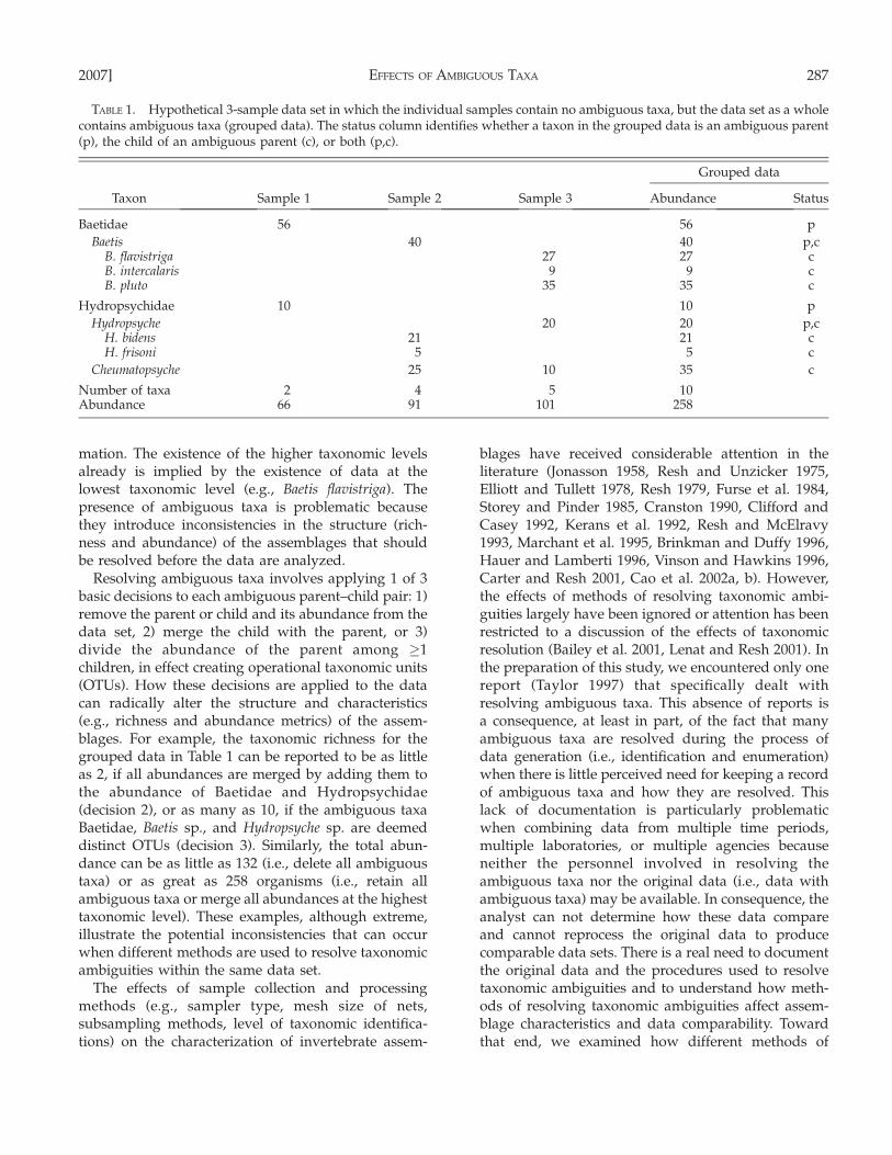
mation. The existence of the higher taxonomic levelsalready is implied by the existence of data at thelowest taxonomic level (e.g., Baetis flavistriga). Thepresence of ambiguous taxa is problematic becausethey introduce inconsistencies in the structure (rich-ness and abundance) of the assemblages that shouldbe resolved before the data are analyzed.

Resolving ambiguous taxa involves applying 1 of 3basic decisions to each ambiguous parent–child pair: 1)remove the parent or child and its abundance from thedata set, 2) merge the child with the parent, or 3)divide the abundance of the parent among �1children, in effect creating operational taxonomic units(OTUs). How these decisions are applied to the datacan radically alter the structure and characteristics(e.g., richness and abundance metrics) of the assem-blages. For example, the taxonomic richness for thegrouped data in Table 1 can be reported to be as littleas 2, if all abundances are merged by adding them tothe abundance of Baetidae and Hydropsychidae(decision 2), or as many as 10, if the ambiguous taxaBaetidae, Baetis sp., and Hydropsyche sp. are deemeddistinct OTUs (decision 3). Similarly, the total abun-dance can be as little as 132 (i.e., delete all ambiguoustaxa) or as great as 258 organisms (i.e., retain allambiguous taxa or merge all abundances at the highesttaxonomic level). These examples, although extreme,illustrate the potential inconsistencies that can occurwhen different methods are used to resolve taxonomicambiguities within the same data set.

The effects of sample collection and processingmethods (e.g., sampler type, mesh size of nets,subsampling methods, level of taxonomic identifica-tions) on the characterization of invertebrate assem-

blages have received considerable attention in theliterature (Jonasson 1958, Resh and Unzicker 1975,Elliott and Tullett 1978, Resh 1979, Furse et al. 1984,Storey and Pinder 1985, Cranston 1990, Clifford andCasey 1992, Kerans et al. 1992, Resh and McElravy1993, Marchant et al. 1995, Brinkman and Duffy 1996,Hauer and Lamberti 1996, Vinson and Hawkins 1996,Carter and Resh 2001, Cao et al. 2002a, b). However,the effects of methods of resolving taxonomic ambi-guities largely have been ignored or attention has beenrestricted to a discussion of the effects of taxonomicresolution (Bailey et al. 2001, Lenat and Resh 2001). Inthe preparation of this study, we encountered only onereport (Taylor 1997) that specifically dealt withresolving ambiguous taxa. This absence of reports isa consequence, at least in part, of the fact that manyambiguous taxa are resolved during the process ofdata generation (i.e., identification and enumeration)when there is little perceived need for keeping a recordof ambiguous taxa and how they are resolved. Thislack of documentation is particularly problematicwhen combining data from multiple time periods,multiple laboratories, or multiple agencies becauseneither the personnel involved in resolving theambiguous taxa nor the original data (i.e., data withambiguous taxa) may be available. In consequence, theanalyst can not determine how these data compareand cannot reprocess the original data to producecomparable data sets. There is a real need to documentthe original data and the procedures used to resolvetaxonomic ambiguities and to understand how meth-ods of resolving taxonomic ambiguities affect assem-blage characteristics and data comparability. Towardthat end, we examined how different methods of

TABLE 1. Hypothetical 3-sample data set in which the individual samples contain no ambiguous taxa, but the data set as a wholecontains ambiguous taxa (grouped data). The status column identifies whether a taxon in the grouped data is an ambiguous parent(p), the child of an ambiguous parent (c), or both (p,c).

Taxon Sample 1 Sample 2 Sample 3

Grouped data

Abundance Status

Baetidae 56 56 p

Baetis 40 40 p,cB. flavistriga 27 27 cB. intercalaris 9 9 cB. pluto 35 35 c

Hydropsychidae 10 10 p

Hydropsyche 20 20 p,cH. bidens 21 21 cH. frisoni 5 5 c

Cheumatopsyche 25 10 35 c

Number of taxa 2 4 5 10Abundance 66 91 101 258

2007] 287EFFECTS OF AMBIGUOUS TAXA

resolving ambiguous taxa affect the comparability ofinvertebrate assemblages, assemblage metrics (rich-ness and abundance), and the interpretation ofinvertebrate responses. Our analyses are based ondata collected by the US Geological Survey’s (USGS)National Water-Quality Assessment (NAWQA) Pro-gram as part of the national urban streams program.

Methods

In the present paper, higher taxonomic levels refer tolevels closer to phylum and lower levels are thosecloser to species. Ambiguous parents (e.g., Baetidae inTable 1) are taxa for which abundances also arereported at lower levels in the taxonomic hierarchy(e.g., B. flavistriga). The taxa at these lower taxonomiclevels (e.g., B. flavistriga, B. intercalaris, and B. pluto) arechildren of the ambiguous parent (Baetidae). A taxoncan be both an ambiguous parent and the child of anambiguous parent if abundances are reported at higherand lower levels of the taxonomic hierarchy (e.g.,Baetis sp. and Hydropsyche sp. in Table 1). A samplemay contain one or more ambiguous parent–childpairings (grouped data) or none at all (samples 1–3).Even when the individual samples do not containambiguous taxa, the data set as a whole may containambiguous parents and children. For example, thesamples presented in Table 1 contain no ambiguoustaxa, but when considered as a group (grouped data)the data set contains 4 ambiguous parents (Baetidae,Baetis sp., Hydropsychidae, and Hydropsyche sp.) and 6children. The consequence is that the determination oftaxa richness for each individual sample in Table 1 isstraight forward and noncontroversial, but estimatingtaxa richness for the entire data set is less so becauseambiguous parents were counted as components oftaxa richness in the individual samples. This conse-quence raises a variety of issues, such as whether taxarichness for the data set should be the total of alltaxonomic entities in the individual samples (10) oronly the nonambiguous entities (6) and whetherconsideration of only nonambiguous entities shouldbe extended to the estimation of taxa richness for theindividual samples to ensure consistency across thedata set. How these issues are handled can determinewhether the data set can support the study objectives(e.g., characterization of richness or abundance met-rics) or analytical methods (e.g., methods that rely oncomparing assemblages: ordination, cluster analysis,discriminant analysis). To address these and otherissues, the techniques for resolving ambiguous taxainclude methods that resolve ambiguities in individualsamples and methods that resolve ambiguities across agroup of samples (i.e., grouped data).

Methods for resolving ambiguous taxa

The 16 methods for resolving taxonomic ambiguitiesthat we examined (Table 2) are variations on 4 generalmethods that embody the decisions (i.e, remove,merge, or distribute taxa) that are commonly usedwhen resolving ambiguous parent–child pairs. Thesegeneral methods are: 1) remove parents, keep children(RPKC), 2) merge children with parent (MCWP), 3)remove parent or merge children with parent (RPMC),and 4) distribute parent among children (DPAC).

These methods resolve ambiguities by consideringall ambiguous parent–child pairs starting with genus(ambiguous parent) and species (children) and pro-gressing though order (O) and family (F) up to phylum(P) and class. These methods can be used to resolvetaxonomic ambiguities separately for each sample (S)or collectively for a group of samples (G). Several ofthese methods (MCWP-S, RPKC-G, MCWP-G, andDPAC-G) have additional variations that addressunique properties of the method (e.g., conservative[C], knowledge based [K], and liberal [L]; Table 2).Details on how these 16 methods resolve ambiguoustaxa are provided in the Appendix and in Cuffney(2003).

The methods of resolving ambiguous taxa describedhere are computationally complex and not amenableto hand calculation when dealing with large numbersof samples and taxa. Consequently, computer software(Invertebrate Data Analysis System [IDAS]) wasdeveloped to automate the process of resolvingtaxonomic ambiguities and to provide other tools forprocessing and analyzing invertebrate data. A detailedexplanation of this software and examples of its use inresolving taxonomic ambiguities and processing in-vertebrate data are given in Cuffney (2003). Data wereprocessed with version 3.7.5 of IDAS. Terrestrial adultswere removed from the data, aquatic life stages werecombined, abundances were converted to densities(/m2), the lowest taxonomic level was set to species,and the data included OTUs, i.e., provisional andconditional identifications (Moulton et al. 2000).

Invertebrate data sets

Data from 4 urban stream studies in the NAWQAProgram (Boston, Massachusetts [BOS]; Raleigh, NorthCarolina [RAL]; Birmingham, Alabama [BIR], and SaltLake City, Utah [SLC]) were used to assess the effectsof different methods of resolving ambiguous taxa onthe characterization, analysis, and interpretation ofresponses along gradients of urban intensity. These 4studies are part of an ongoing program that comparesbiological, chemical, and physical responses alonggradients of urban intensity in major metropolitan

288 [Volume 26T. F. CUFFNEY ET AL.

areas across the USA. The intensity of urbanization isdefined by a multimetric urban intensity index (UII)derived from a combination of land-cover, landuse,infrastructure, population, and socioeconomic vari-ables (McMahon and Cuffney 2000, Coles et al. 2004,Cuffney et al. 2005, Tate et al. 2005). These studies wereconducted by using a common study design (Coleset al. 2004, Cuffney et al. 2005, Tate et al. 2005) andcommon sampling (Cuffney et al. 1993 for BIR, BOS,SLC, Moulton et al. 2002 for RAL) and processingprotocols (Moulton et al. 2000). All invertebratesamples were processed by the USGS National Water-Quality Laboratory (NWQL) in Denver, Colorado.

Assessing the effects of resolving ambiguous taxa

The effects of the use of different methods to resolveambiguous taxa were evaluated by 2 approaches. The

1st approach examined changes to the structure of theassemblages (i.e., similarity among assemblages), thevalues of assemblage metrics, and the relations amongsites (i.e., the degree to which the structure of theoriginal data is preserved). The 2nd approach evaluat-ed effects on the interpretation of invertebrate respons-es to urbanization, an environmental disturbance thatstrongly degrades invertebrate assemblages (Paul andMeyer 2001, Coles et al. 2004, Carter and Fend 2005,Cuffney et al. 2005). Together, these 2 approachesaddress important issues related to data comparability,consistency, and interpretation.

Effects on assemblage structure were tested by a 2-stage similarity analysis (2STAGE, Primer 6; PRIMER-E, Plymouth, UK). The 16 methods for resolvingambiguous taxa were applied to the original data(ORIG) for each of the 4 urban studies (BIR, BOS, RAL,

TABLE 2. Descriptions of the methods used to resolve taxonomic ambiguities and the abbreviations that identify each method.The basic methods are identified by 4-character abbreviations. Variants of each method are identified by a 1- or 2-character suffix.See the Appendix for detailed descriptions of each method. S ¼ single, G ¼ grouped, F ¼ family, O ¼ order, P ¼ phylum, C ¼conservative, K ¼ knowledge based, L ¼ liberal.

Method Description

ORIG Original data with ambiguous taxa

Basic methods

RPKC Remove parent, keep children: remove the ambiguous parents, but keep the children of the ambiguousparents (parent’s abundances are lost)

Variants: RPKC-S, RPKC-GC, RPKC-GK, RPKC-GLMCWP Merge children with parent: add the abundances of the children to the abundance of the associated

ambiguous parentVariants: MCWP-S, MCWP-GF, MCWP-GO, MCWP-GP

RPMC Remove parent or merge children: remove the ambiguous parent if the sum of the children’s abundances isgreater than the parent’s abundance (RPKC); otherwise, merge the children with the parent (MCWP)

Variants: RPMC-S, RPMC-GDPAC Distribute parent among children: distribute the abundance of the ambiguous parent among the associated

children in proportion to the relative abundance of each child in the sample (-S variants) or grouped data(-G variants).

Variants: DPAC-S, DPAC-GC, DPAC-GK, DPAC-GL

Variants that apply to all methods

-S Resolve ambiguous taxa separately for each sample-G Resolve ambiguous taxa for a group of samples. The rules for resolving ambiguous taxa are derived by

applying the -S variant to the grouped data (sum of all samples) and then applying these rules to eachsample individually

MWCP-S and MWCP-G variants

-F Family variant: remove all ambiguous parents above the level of family before resolving ambiguous taxa-O Order variant: remove all ambiguous parents above the level of order before resolving ambiguous taxa-P Phylum variant: remove all ambiguous parents above the level of phylum before resolving ambiguous taxa

(i.e., retain all ambiguous parents)

RPKC-G and DPAC-G variants

-C Conservative: if the ambiguous parent has no child in a sample, substitute the most frequently occurringchild for the parent (i.e., assign the parent’s abundance to the child)

-K Knowledge based: if the ambiguous parent has no child in a sample, substitute one or more children on thebasis of knowledge of taxa distributions and assemblage characteristics at similar sites

-L Liberal: if the ambiguous parent has no child in a sample, substitute all of the children associated with theparent in the grouped data


SLC) to produce a site-by-taxa matrix for each methodand each study (16 methods þ ORIG 3 4 studies ¼ 68data matrices). Abundance data in each site-by-taxamatrix were

ffiffiffiffiffiffiffiðxÞ

ptransformed to reduce the influence

of extreme values and a site-by-site similarity matrixwas calculated by Bray–Curtis similarity. Spearmanrank correlations were then calculated between allpairs of similarity matrices representing ORIG and the16 methods for resolving taxonomic ambiguities. Thisproduced a method-by-method (17 3 17) correlationmatrix that was used in a 2nd-stage nonmetricmultidimensional scaling (NMDS) plot to give aseparate graphical representation of the similaritiesamong methods for each study (BIR, BOS, RAL, andSLC). A second 2STAGE similarity analysis was usedto determine how closely the method-by-methodcorrelation matrices derived for each study resembledone another. This comparison was accomplished byusing the method-by-method correlation matricesderived for each study as input into the 2STAGEanalysis to obtain a correlation matrix that representedthe correlation among studies based on the correlationamong methods.

The effects of resolving taxonomic ambiguities onassemblage metrics were investigated for 34 metrics(Table 3) commonly used in bioassessment studies(Barbour et al. 1999). Metrics derived from ORIG,which contained unresolved ambiguous taxa (e.g.,Baetidae, Baetis sp., and B. pluto are 3 taxa in ORIG),were compared to metrics derived from assemblagescreated by applying each of the 16 methods to ORIG.Comparisons were based on the value of the metricexpressed as a percentage of the value for ORIG. For

example, the metric Ephemeroptera þ Plecoptera þTrichoptera richness (EPTr) comparisons would beexpressed as % ORIG ¼ ([EPTr from RPMC-S]/[EPTrfrom ORIG] 3 100) and as the correlation (q) withORIG (e.g., correlation between EPTr from RPMC-Sand EPTr from ORIG). Separate analyses were con-ducted for each of the 4 studies. The % ORIG measuresthe extent to which the method changes the value ofthe metric relative to ORIG while minimizing thedifferences in metric values among sites. In contrast,the correlation with ORIG measures how consistentlythe method changes the value of the metric across allsites in a study. A large difference in % ORIG betweenmethods indicates that the methods do not generatecomparable results. Methods that show weak correla-tions with ORIG or high variability (i.e., coefficient ofvariation [CV] of the correlations derived for allmetrics for all 4 studies) do not operate in a consistentmanner across all sites and studies. Consequently,differences among sites may be an artifact of themethod used to resolve ambiguous taxa rather thanresponses to environmental changes.

Effects on the interpretation of responses alongurban gradients were investigated by indirect gradientanalysis (Gauch 1982) and correlation analysis. Indi-rect gradient analysis uses the correlation betweenordination site scores and urban intensity to determinehow strongly changes in urbanization are associatedwith changes in assemblages (Coles et al. 2004,Cuffney et al. 2005). Correspondence analysis (CA)was used to obtain ordination site scores along theprimary ordination axis (CANOCO, version 4.5;Microcomputer Power, Ithaca, New York). These

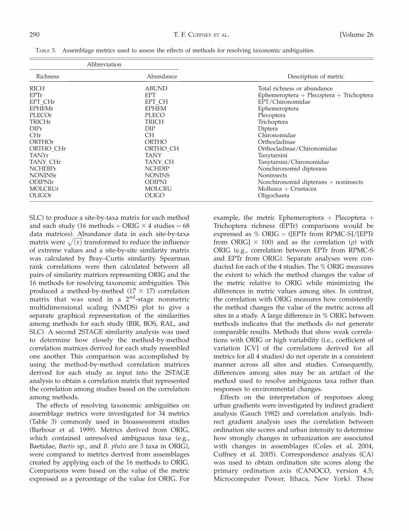
TABLE 3. Assemblage metrics used to assess the effects of methods for resolving taxonomic ambiguities.

Abbreviation

Description of metricRichness Abundance

RICH ABUND Total richness or abundanceEPTr EPT Ephemeroptera þ Plecoptera þ TrichopteraEPT_CHr EPT_CH EPT/ChironomidaeEPHEMr EPHEM EphemeropteraPLECOr PLECO PlecopteraTRICHr TRICH TrichopteraDIPr DIP DipteraCHr CH ChironomidaeORTHOr ORTHO OrthocladinaeORTHO_CHr ORTHO_CH Orthocladinae/ChironomidaeTANYr TANY TanytarsiniTANY_CHr TANY_CH Tanytarsini/ChironomidaeNCHDIPr NCHDIP Nonchironomid dipteransNONINSr NONINS NoninsectsODIPNIr ODIPNI Nonchironomid dipterans þ noninsectsMOLCRUr MOLCRU Mollusca þ CrustaceaOLIGOr OLIGO Oligochaeta


scores represent ecological distances among sites basedon differences in assemblage structure. Abundancedata (/m2) were

ffiffiffiffiffiffiffiðxÞ

ptransformed to reduce the

influence of extreme values and rare taxa weredownweighted to prevent them from distorting theordination (Hill 1979). Correlation (Spearman rank)analysis was used to assess the strength of theassociation between UII, ordination site scores, andeach of the 34 assemblage metrics derived for eachmethod. Spearman rank correlations (q) were calcu-lated by Systat 9.0 (SPSS, Chicago, Illinois). Consis-tency in the correlations between metrics and UII wasused to assess consistency among methods by corre-lating (q) the correlations between metrics and UIIobtained from a particular method (e.g., RPMC-S) withthe correlations between UII and the correspondingmetrics obtained from ORIG (i.e., the correlations withUII for the 17 metrics were correlated with thecorresponding correlations with UII derived fromORIG). Consistency was evaluated for each of the 4studies. Strong correlations indicate that the methodoperated consistently over all samples and metrics andmethodological differences should not be a factor ininterpreting the response to environmental changes(i.e., urbanization).

Results

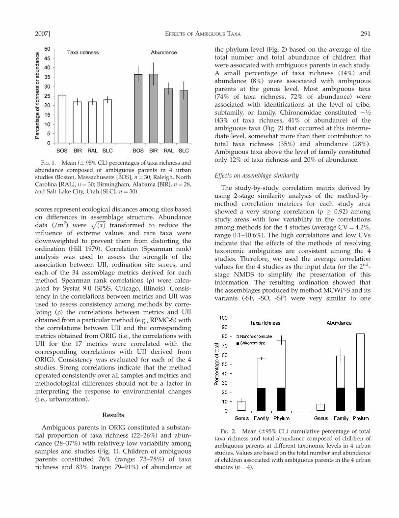
Ambiguous parents in ORIG constituted a substan-tial proportion of taxa richness (22–26%) and abun-dance (28–37%) with relatively low variability amongsamples and studies (Fig. 1). Children of ambiguousparents constituted 76% (range: 73–78%) of taxarichness and 83% (range: 79–91%) of abundance at

the phylum level (Fig. 2) based on the average of thetotal number and total abundance of children thatwere associated with ambiguous parents in each study.A small percentage of taxa richness (14%) andabundance (8%) were associated with ambiguousparents at the genus level. Most ambiguous taxa(74% of taxa richness, 72% of abundance) wereassociated with identifications at the level of tribe,subfamily, or family. Chironomidae constituted ;½(43% of taxa richness, 41% of abundance) of theambiguous taxa (Fig. 2) that occurred at this interme-diate level, somewhat more than their contribution tototal taxa richness (35%) and abundance (28%).Ambiguous taxa above the level of family constitutedonly 12% of taxa richness and 20% of abundance.

Effects on assemblage similarity

The study-by-study correlation matrix derived byusing 2-stage similarity analysis of the method-by-method correlation matrices for each study areashowed a very strong correlation (q � 0.92) amongstudy areas with low variability in the correlationsamong methods for the 4 studies (average CV¼ 4.2%,range 0.1–10.6%). The high correlations and low CVsindicate that the effects of the methods of resolvingtaxonomic ambiguities are consistent among the 4studies. Therefore, we used the average correlationvalues for the 4 studies as the input data for the 2nd-stage NMDS to simplify the presentation of thisinformation. The resulting ordination showed thatthe assemblages produced by method MCWP-S and itsvariants (-SF, -SO, -SP) were very similar to one

FIG. 2. Mean (695% CL) cumulative percentage of totaltaxa richness and total abundance composed of children ofambiguous parents at different taxonomic levels in 4 urbanstudies. Values are based on the total number and abundanceof children associated with ambiguous parents in the 4 urbanstudies (n ¼ 4).

FIG. 1. Mean (6 95% CL) percentages of taxa richness andabundance composed of ambiguous parents in 4 urbanstudies (Boston, Massachusetts [BOS], n¼ 30; Raleigh, NorthCarolina [RAL], n¼ 30; Birmingham, Alabama [BIR], n¼ 28,and Salt Lake City, Utah [SLC], n ¼ 30).


another, but they were so different from other

assemblages that they obscured the relations among

the other methods. For this reason, the analyses were

repeated after removing the MCWP-S methods.

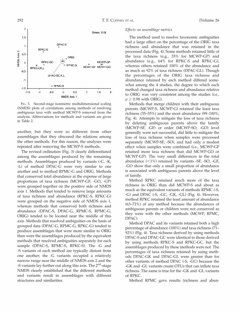
The revised ordination (Fig. 3) clearly differentiated

among the assemblages produced by the remaining

methods. Assemblages produced by variants (-C, -K,

-L) of method DPAC-G were very similar to one

another and to method RPMC-G and ORIG. Methods

that conserved total abundance at the expense of large

proportions of taxa richness (MCWP-GF, -GO, -GP)

were grouped together on the positive side of NMDS

axis 1. Methods that tended to remove large amounts

of taxa richness and abundance (RPKC-S, RPKC-G)

were grouped on the negative side of NMDS axis 1,

whereas methods that conserved both richness and

abundance (DPAC-S, DPAC-G, RPMC-S, RPMC-G,

ORIG) tended to be located near the middle of this

axis. Methods that resolved ambiguities on the basis of

grouped data (DPAC-G, RPMC-G, RPKC-G) tended to

produce assemblages that were more similar to ORIG

than were the assemblages produced by the equivalent

methods that resolved ambiguities separately for each

sample (DPAC-S, RPMC-S, RPKC-S). The -G and

-S variants of each method are typically distant from

one another; the -G variants occupied a relatively

narrow range near the middle of NMDS axis 2 and the

-S variants lay further out along this axis. The 2nd-stage

NMDS clearly established that the different methods

and variants result in assemblages with different

structures and similarities.

Effects on assemblage metrics

The method used to resolve taxonomic ambiguitieshad a large effect on the percentage of the ORIG taxarichness and abundance that was retained in theprocessed data (Fig. 4). Some methods retained little ofthe taxa richness (e.g., 35% for MCWP-GP) andabundance (e.g., 64% for RPKC-S and RPKC-G),whereas others retained 100% of the abundance andas much as 92% of taxa richness (DPAC-GL). Thoughthe percentages of the ORIG taxa richness andabundance retained by each method differed some-what among the 4 studies, the degree to which eachmethod changed taxa richness and abundance relativeto ORIG was very consistent among the studies (i.e.,q � 0.98 with ORIG).

Methods that merge children with their ambiguousparents (MCWP-S, MCWP-G) retained the least taxarichness (35–55%) and the most abundance (99–100%;Fig. 4). Attempts to mitigate the loss of taxa richnessby deleting ambiguous parents above the family(MCWP-SF, -GF) or order (MCWP-SO, -GO) levelgenerally were not successful, did little to mitigate theloss of taxa richness when samples were processedseparately (MCWP-SF, -SO), and had only a modesteffect when samples were combined (i.e., MCWP-GFretained more taxa richness than did MCWP-GO orMCWP-GP). The very small differences in the totalabundance (,1%) retained by variants -SF, -SO, -GF,-GO show that only a small proportion of abundanceis associated with ambiguous parents above the levelof family.

Method RPKC retained much more of the taxarichness in ORIG than did MCWP-S and about asmuch as the equivalent variants of methods RPMC (-S,-G) and DPAC (-S, -GC, -GK, -GL) (Fig. 4). However,method RPKC retained the least amount of abundance(63–72%) of any method because the abundances ofambiguous parents or children were not conserved asthey were with the other methods (MCWP, RPMC,DPAC).

Method DPAC and its variants retained both a highpercentage of abundance (100%) and taxa richness (71–92%) (Fig. 4). Taxa richness derived by using methodsDPAC-S and DPAC-GC were identical to those derivedby using methods RPKC-S and RPKC-GC, but theassemblages produced by these methods were not. Thepercentages of taxa richness retained by using meth-ods DPAC-GK and DPAC-GL were greater than forother variants of method DPAC (-S, -GC) because the-GK and -GL variants create OTUs that can inflate taxarichness. The same is true for the -GK and -GL variantsof RPKC.

Method RPMC gave results (richness and abun-

FIG. 3. Second-stage nonmetric multidimensional scaling(NMDS) plots of correlations among methods of resolvingambiguous taxa with method MCWP-S removed from theanalysis. Abbreviations for methods and variants are givenin Table 2.


dance) that were intermediate to those obtained byusing methods RPKC and DPAC (Fig. 4). It retainedslightly less taxa richness (71–78%) than did methodsRPKC and DPAC (74–92%) and an intermediate levelof abundance (83–94%) compared to RPKC (64–72%)and DPAC (100%). This result was expected becauseRPMC resolves ambiguous parent–child pairs byapplying either method RPKC or DPAC dependingupon whether the parent’s abundance is greater thanthe collective abundance of the children.

The values of other richness (Table 4) and abun-dance (Table 5) metrics also were affected strongly bythe method used to resolve taxonomic ambiguities.Some methods (MCWP-GF, -GO, and -GP) eliminatedthe taxonomic groups required to calculate the metric(e.g., ORTHOr, ORTHO_CHr, TANYr, TANY_CHr, inTable 4; ORTHO, ORTH_CH, TANY, TANY_CH inTable 5; see Table 3 for metric abbreviations). Others,particularly metrics based on ratios, reached valuesthat were multiples of the value in ORIG. This patternwas most evident for richness metrics (e.g., EPT_CHrwith method MCWP, TANY_CHr with methodsRPKC, RPMC, and DPAC; Table 4), though there weresimilar examples among the abundance metrics (e.g.,TANY_CH with methods RPKC, RPMC, and DPAC;Table 5). Most of the richness (13 of 16) and abundance(11 of 16) metrics followed the pattern previously

described for total richness (RICH in Table 4) orabundance (ABUND in Table 5) as indicated by astrong correlation (jqj � 0.8) with RICH or ABUND.However, only 8 (EPT, EPHEM, PLECO, TRICHO,DIP, CH, NCDIP, and ODIPNI) of the 16 metrics werestrongly correlated with both RICH and ABUND. Thestrong influence of the method used to resolveambiguous taxa on the values of metrics suggests thatmetrics from different sources should be combinedonly if there is a clear understanding of the compara-bility of the methods used to resolve ambiguous taxa.

Although the method used to resolve ambiguoustaxa had a strong effect on the values of metrics, theseeffects were consistent among methods as evidencedby strong average correlations (q � 0.88) betweenmetrics derived from ORIG and metrics derived fromall methods except MCWP (Table 6). Average correla-tions for richness metrics derived by using methodMCWP generally were much lower (0.53–0.82) than forother methods and correlations for some metrics couldnot be calculated (e.g., ORTHOr, ORTHO_CHr,TANYr, TANY_CHr) because the method (MCWP-GF, -GO, -GP) eliminated the taxa required to calculatethe metric. Correlations for abundance metrics derivedby using method MCWP were much higher than theequivalent richness metric. Variations of MCWP thatdelete ambiguous parents above the family (-SF, -GF)

FIG. 4. Taxa richness (Rich) and abundance (Abund) for the Birmingham (BIR), Boston (BOS), Raleigh (RAL), and Salt Lake City(SLC) urban studies after resolving taxonomic ambiguities. Data are expressed as the average percentage (695% CL) of the taxarichness or abundance in the original data (ORIG). Abbreviations for the methods and variants used to resolve ambiguous taxa aregiven in Table 2.


TA

BL

E4.

Ric

hn

ess

met

rics

der

ived

usi

ng

each

of

the

16m

eth

od

sfo

rre

solv

ing

tax

on

om

icam

big

uit

ies

and

exp

ress

edas

the

aver

age

per

cen

tag

eo

fth

ev

alu

ein

the

ori

gin

ald

ata

(OR

IG)

for

the

4u

rban

stu

die

s.M

etri

csm

ark

edw

ith

anas

teri

sk(*

)w

ere

stro

ng

lyco

rrel

ated

(jqj�

0.8)

wit

hto

tal

tax

ari

chn

ess

(RIC

H).

Ab

bre

via

tio

ns

for

met

ho

ds

and

var

ian

tso

fre

solv

ing

amb

igu

ou

sta

xa

are

giv

enin

Tab

le2.

Ab

bre

via

tio

ns

for

asse

mb

lag

em

etri

csar

eg

iven

inT

able

3.N

C¼

met

ric

cou

ldn

ot

be

calc

ula

ted

.

Met

ho

dan

dv

aria

nt

RP

KC

MC

WP

MC

WP

MC

WP

RP

MC

DP

AC

RP

KC

RP

KC

RP

KC

MC

WP

MC

WP

MC

WP

RP

MC

DP

AC

DP

AC

DP

AC

Met

ric

-S-S

F-S

O-S

P-S

-S-G

C-G

K-G

L-G

F-G

O-G

P-G

-GC

-GK

-GL

RIC

H77

5554

5476

7777

7884

4940

4074

7779

84E

PT

r*66

5452

5263

6666

6883

5236

3661

6668

83E

PT

_CH

r*86

500

468

468

8386

8688

106

651

284

284

8086

8810

6E

PH

EM

r*63

5856

5662

6364

6990

5642

4254

6369

90P

LE

CO

r*83

7873

7381

8383

8611

070

6161

7383

8611

0T

RIC

Hr*

6853

5151

6668

6869

8551

3333

6668

6985

DIP

r*78

3737

3777

7878

7881

2522

2276

7878

81C

Hr*

7824

2424

7778

7878

8110

88

7678

7882

OR

TH

Or*

8216

1616

8082

8285

94N

CN

CN

C80

8285

95O

RT

HO

_CH

r*10

631

3131

105

106

106

108

109

NC

NC

NC

105

106

108

109

TA

NY

r*97

1616

1697

9797

9797

NC

NC

NC

9797

9797

TA

NY

_CH

r*12

729

2929

128

127

127

126

123

NC

NC

NC

129

127

126

123

NC

DIP

r*77

7776

7677

7778

7981

7154

5475

7879

81N

ON

INS

r90

8989

8890

9090

9296

8888

8687

9093

96O

DIP

NIr

*85

8484

8385

8586

8790

8175

7382

8687

90M

OL

CR

Ur

8180

7977

8081

8185

9476

7673

7281

8694

OL

IGO

r10

010

010

010

010

010

010

010

010

010

010

010

010

010

010

010

0


TA

BL

E5.

Ab

un

dan

cem

etri

csd

eriv

edu

sin

gea

cho

fth

e16

met

ho

ds

for

reso

lvin

gta

xo

no

mic

amb

igu

itie

san

dex

pre

ssed

asth

eav

erag

ep

erce

nta

ge

of

the

val

ue

inth

eo

rig

inal

dat

a(O

RIG

)fo

rth

e4

urb

anst

ud

ies.

Met

rics

mar

ked

wit

han

aste

risk

(*)

wer

est

ron

gly

corr

elat

ed(jqj�

0.8)

wit

hto

tal

abu

nd

ance

(AB

UN

D).

Ab

bre

via

tio

ns

for

met

ho

ds

and

var

ian

tso

fre

solv

ing

amb

igu

ou

sta

xa

are

giv

enin

Tab

le2.

Ab

bre

via

tio

ns

for

asse

mb

lag

em

etri

csar

eg

iven

inT

able

3.N

C¼

met

ric

cou

ldn

ot

be

calc

ula

ted

.

Met

ho

dan

dv

aria

nt

RP

KC

MC

WP

MC

WP

MC

WP

RP

MC

DP

AC

RP

KC

RP

KC

RP

KC

MC

WP

MC

WP

MC

WP

RP

MC

DP

AC

DP

AC

DP

AC

Met

ric

-S-S

F-S

O-S

P-S

-S-G

C-G

K-G

L-G

F-G

O-G

P-G

-GC

-GK

-GL

AB

UN

D67

100

100

100

8910

067

6767

9910

010

088

100

100

100

EP

T*

6310

010

010

083

100

6363

6310

010

010

080

100

100

100

EP

T_C

H75

100

9999

9310

075

7575

100

7474

8910

010

010

0E

PH

EM

*62

9910

010

082

100

6262

6299

100

100

7210

010

010

0P

LE

CO

*77

9310

010

089

100

7777

7788

100

100

8310

010

010

0T

RIC

H*

6610

010

010

085

100

6666

6610

010

010

084

100

100

100

DIP

*76

100

100

100

9210

076

7676

100

100

100

9210

010

010

0C

H*

8610

099

9990

100

8686

8610

074

7490

100

100

100

OR

TH

O81

3939

3987

102

8181

81N

CN

CN

C87

102

102

102

OR

TH

O_C

H93

3939

3997

102

9393

93N

CN

CN

C97

102

102

102

TA

NY

9916

1616

9911

099

9999

NC

NC

NC

9911

011

011

0T

AN

Y_C

H11

716

1616

112

110

117

117

117

NC

NC

NC

111

110

110

110

NC

DIP

*58

100

9999

9610

058

5858

100

7474

9610

010

010

0N

ON

INS

*87

9999

100

9810

087

8787

9899

100

9310

010

010

0O

DIP

NI*

6999

9999

9810

069

6969

9983

8495

100

100

100

MO

LC

RU

*73

9697

100

9410

073

7373

9394

100

8010

010

010

0O

LIG

O*

100

100

100

100

100

100

100

100

100

100

100

100

100

100

100

100


and order levels (-SO, -GO) did not produce strongercorrelations with ORIG or mitigate problems with thecalculation of some metrics. Correlations betweenmetrics derived from the -S variants of MCWP andthe ORIG data were much lower than those for the-G variants indicating that the -G variants retainedmore of the structure of the original data than did the-S variants.

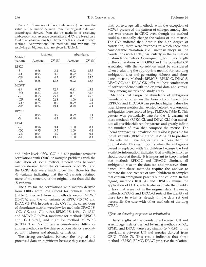
The CVs for the correlations with metrics derivedfrom ORIG were low (,5%) for richness metrics(Table 6) derived from all methods except MCWP(23–75%) and the -L variants of RPKC (13.5%) andDPAC (13.8%). In contrast the CVs for the correlationsof abundance metrics were low for methods DPAC (-S,-GC, -GK, and -GL: ,1%), RPMC (-S: 1.4%, -G: 1.3%)and MCWP-G (,7%), moderate for methods RPKC-Sand -G (15.3%), and high for method MCWP-S(45.3%). The CVs indicate a considerable differenceamong methods in the degree of consistency associat-ed with richness and abundance metrics.

The strong correlations between the original andprocessed data are significant because they established

that, on average, all methods with the exception ofMCWP preserved the pattern of changes among sitesthat was present in ORIG even though the methodcould substantially change the values of the metrics.The CVs indicate that, despite the high degree ofcorrelation, there were instances in which there wasconsiderable variation (i.e., inconsistency) in thecorrelations with ORIG, particularly in the estimationof abundance metrics. Consequently, both the strengthof the correlations with ORIG and the potential CVassociated with that correlation must be consideredwhen evaluating the appropriate method for resolvingambiguous taxa and generating richness and abun-dance metrics. Methods RPMC-S, RPMC-G, DPAC-S,DPAC-GC, and DPAC-GK offer the best combinationof correspondence with the original data and consis-tency among metrics and study areas.

Methods that assign the abundance of ambiguousparents to children on the basis of combined data(RPKC-G and DPAC-G) can produce higher values fortaxa richness metrics than existed before the taxonomicambiguities were resolved (e.g., PLECOr; Table 4). Thispattern was particularly true for the -L variants ofthese methods (RPKC-GL and DPAC-GL) that substi-tute all possible children for parents and greatly inflatethe number of taxa that compose the metric. Theliberal approach is unrealistic, but it also is possible forthe -K variants (RPKC-GK and DPAC-GK) to producedata sets that have higher taxa richness than theoriginal data. This result occurs when the ambiguousparent is replaced with �2 children because the bestavailable information indicates that multiple childrenshould occur at the site. It is important to keep in mindthat methods RPKC-G and DPAC-G eliminate allambiguous taxa in the data set and preserve abun-dance, but these methods require the analyst toestimate the occurrences of taxa (children) in samplesthat contain ambiguous parents but no children. In thisregard, methods RPKC-G and DPAC-G mimic theapplication of OTUs, which also estimate the identityof taxa that were not in the original data. However,methods RPKG-G and DPAC-G restrict the identity ofthese taxa to what is already in the data set (notnecessarily the case with other methods of derivingOTUs).

Effects on detecting responses to urbanization

The strengths of the correlations between UII andassemblage metrics derived by using methods RPKC,RPMC, and DPAC were very similar (q � 0.94) to thecorrelations between UII and metrics derived fromORIG (Table 7). This result indicates that thesemethods (RPKC, RPMC, DPAC) preserve the relations

TABLE 6. Summary of the correlations (q) between thevalue of the metric derived from the original data andassemblages derived from the 16 methods of resolvingambiguous taxa. Average correlation and CV are based on atotal of 68 observations (i.e., 17 metrics 3 4 studies) for eachmethod. Abbreviations for methods and variants forresolving ambiguous taxa are given in Table 2.

Metric/variant

Richness Abundance

Average CV (%) Average CV (%)

RPKC

-S 0.96 3.4 0.92 15.3-GC 0.95 3.5 0.92 15.3-GK 0.94 4.7 0.92 15.3-GL 0.88 13.5 0.92 15.3

MCWP

-SF 0.57 72.7 0.81 45.3-SO 0.53 75.3 0.81 45.3-SP 0.53 75.2 0.81 45.3-GF 0.82 22.8 1.00 1.1-GO 0.75 30.0 0.99 6.4-GP 0.74 29.4 0.99 6.4

RPMC

-S 0.95 3.9 0.99 1.4-G 0.94 4.4 0.99 1.3

DPAC

-S 0.96 3.4 1.00 0.1-GC 0.95 3.5 1.00 0.1-GK 0.94 4.9 1.00 0.1-GL 0.88 13.8 1.00 0.1


among samples that existed in ORIG. Correlationsbetween UII and metrics derived by using methodMCWP and its variants were not always similar to thecorrelation between UII and metrics derived fromORIG. That is, method MCWP did not alwayspreserve the relations among samples that existed inORIG. The range between the best and worstcorrelations with UII all were associated with differ-ences between metrics derived by using variations ofmethod MCWP and those derived by using methodsRPKC, RPMC, or DPAC. Resolving ambiguous taxaseparately (-S) or for a group of samples (-G) had littleeffect on the correlation between the metric and urbanintensity for methods RPKC, RPMC, and DPAC.However, resolving ambiguous taxa for a group ofsamples (-G) did improve the correspondence betweenMCWP and ORIG, particularly for richness metricsderived by using the -GF variant (MCWP-GF).

The number of richness metrics that were stronglycorrelated (jqj � 0.7) with UII was highly consistent(17–18 metrics) among methods RPKC, RPMC, andDPAC (qUII in Table 7) as were the number (12–13)strongly correlated with both UII and ORIG (qUIIORIG in Table 7). In contrast, method MCWP, with the

exception of MCWP-GF, had fewer richness metricsthat were strongly correlated with UII (8–12) andrelatively few of these metrics (6–9) also were stronglycorrelated with ORIG. The number of metrics thatwere strongly correlated with method MCWP-GFwere much more similar (16 for UII, 11 for both UIIand ORIG) to the other methods than were the -SF,-SO, -GO, and -GP variants of MCWP. Fewerabundance metrics were strongly correlated to UII(2–3) than were richness metrics and most (2–3) ofthese metrics were the same metrics that were stronglycorrelated with UII for the original data (ORIG). Thenumber of metrics that were strongly correlated withUII was relatively small compared to the number ofmetrics that were considered (i.e., 17 metrics 3 4studies ¼ 68).

With the exception of the MCWP methods, theability to detect responses to urbanization by usingmetrics (i.e., jqj � 0.7) was not sensitive to the methodused to resolve taxonomic ambiguities. Compared tothe other methods, the relations with UII obtained byusing MCWP were inconsistent among metrics andstudies, although method MCWP-GF approached thelevels obtained with other methods. This inconsistency

TABLE 7. Summary of the consistency in the correlations between urban intensity (UII) and metrics derived from the 16 methodsof resolving ambiguous taxa. Consistency is expressed as the correspondence (q) between the correlations with UII obtained fromeach method and from the original data (ORIG) (i.e., the correlations with UII for the 17 metrics are correlated with thecorresponding correlations with UII derived from ORIG). The maximum and minimum correlations are based on the correlationobtained for each of the 4 studies. The number of observations that were strongly (jqj � 0.70) correlated with UII (qUII) and stronglycorrelated with both UII and ORIG (qUII ORIG) are based on a total of 68 observations (17 metrics 3 4 study areas) for each method.Abbreviations for methods of resolving ambiguous taxa are explained in Table 2.

Metric/variant

Richness Abundance

Min Max qUIIqUII

ORIG Min Max qUIIqUII

ORIG

RPKC-S 0.98 0.99 17 13 0.94 0.95 2 2-GC 0.98 0.99 17 13 0.94 0.98 2 2-GK 0.98 0.99 17 13 0.94 0.98 2 2-GL 0.97 0.99 18 12 0.94 0.98 2 2

MCWP-SF 0.57 0.84 13 9 0.64 0.95 3 3-SO 0.55 0.85 12 9 0.64 0.95 3 3-SP 0.55 0.85 12 9 0.64 0.95 3 3-GF 0.90 0.97 16 11 0.74 0.94 3 3-GO 0.83 0.94 8 6 0.73 0.94 3 3-GP 0.82 0.94 8 6 0.74 0.94 3 3

RPMC-S 0.98 0.99 17 13 0.99 0.99 3 3-G 0.98 0.99 17 13 0.98 0.99 3 3

DPAC-S 0.98 0.99 17 13 0.99 1.00 3 3-GC 0.98 0.99 17 13 0.99 1.00 3 3-GK 0.98 0.99 17 13 0.99 1.00 3 3-GL 0.97 0.99 18 12 0.99 1.00 3 3


suggests that method MCWP should not be used todetect or interpret responses.

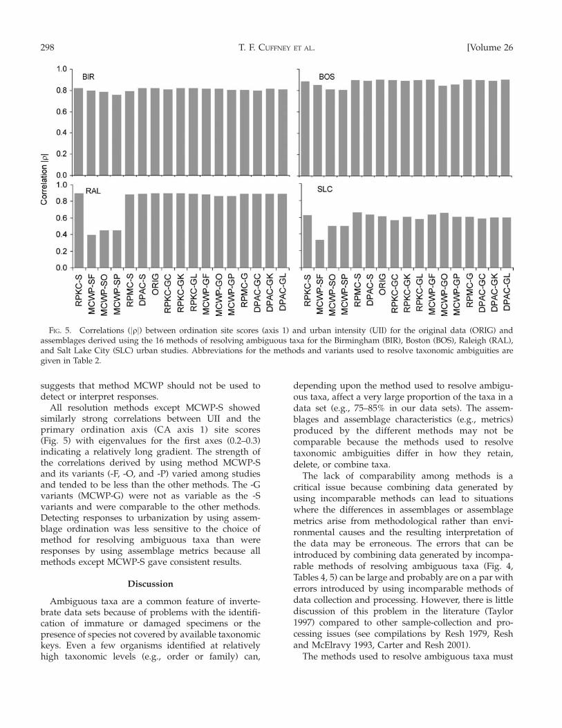
All resolution methods except MCWP-S showedsimilarly strong correlations between UII and theprimary ordination axis (CA axis 1) site scores(Fig. 5) with eigenvalues for the first axes (0.2–0.3)indicating a relatively long gradient. The strength ofthe correlations derived by using method MCWP-Sand its variants (-F, -O, and -P) varied among studiesand tended to be less than the other methods. The -Gvariants (MCWP-G) were not as variable as the -Svariants and were comparable to the other methods.Detecting responses to urbanization by using assem-blage ordination was less sensitive to the choice ofmethod for resolving ambiguous taxa than wereresponses by using assemblage metrics because allmethods except MCWP-S gave consistent results.

Discussion

Ambiguous taxa are a common feature of inverte-brate data sets because of problems with the identifi-cation of immature or damaged specimens or thepresence of species not covered by available taxonomickeys. Even a few organisms identified at relativelyhigh taxonomic levels (e.g., order or family) can,

depending upon the method used to resolve ambigu-ous taxa, affect a very large proportion of the taxa in adata set (e.g., 75–85% in our data sets). The assem-blages and assemblage characteristics (e.g., metrics)produced by the different methods may not becomparable because the methods used to resolvetaxonomic ambiguities differ in how they retain,delete, or combine taxa.

The lack of comparability among methods is acritical issue because combining data generated byusing incomparable methods can lead to situationswhere the differences in assemblages or assemblagemetrics arise from methodological rather than envi-ronmental causes and the resulting interpretation ofthe data may be erroneous. The errors that can beintroduced by combining data generated by incompa-rable methods of resolving ambiguous taxa (Fig. 4,Tables 4, 5) can be large and probably are on a par witherrors introduced by using incomparable methods ofdata collection and processing. However, there is littlediscussion of this problem in the literature (Taylor1997) compared to other sample-collection and pro-cessing issues (see compilations by Resh 1979, Reshand McElravy 1993, Carter and Resh 2001).

The methods used to resolve ambiguous taxa must

FIG. 5. Correlations (jqj) between ordination site scores (axis 1) and urban intensity (UII) for the original data (ORIG) andassemblages derived using the 16 methods of resolving ambiguous taxa for the Birmingham (BIR), Boston (BOS), Raleigh (RAL),and Salt Lake City (SLC) urban studies. Abbreviations for the methods and variants used to resolve taxonomic ambiguities aregiven in Table 2.


be evaluated carefully before data sets can becombined. Thorough documentation of the processused to resolve ambiguous taxa is essential fordetermining whether data are comparable. Unfortu-nately, the procedures used to resolve ambiguous taxagenerally are not well documented and discussion ofthis topic generally is restricted to specifying thedesired taxonomic level for identifications (e.g., Rosen-berg and Resh 1993, Barbour et al. 1999, Bailey et al.2001, Lenat and Resh 2001, Carter and Fend 2005,Kreutzweiser et al. 2005, NCDENR 2006) rather than todocumenting how ambiguous parent–child pairs areresolved. This level of discussion does not providesufficient information to assess adequately whetherassemblages have been processed by using compara-ble methods. Even if the methods of resolvingambiguous taxa are carefully documented, it may notbe possible to modify assemblages so that they arecomparable. For example, assemblages processed byusing methods MCWP and DPAC can not bereprocessed to produce comparable assemblages be-cause the required taxonomic information has beenremoved from the data sets. One means of addressingthis issue is to provide uncensored data sets (i.e., thedata sets with ambiguous taxa) as part of thedocumentation process (Taylor 1997). This practicewould make it possible to form comparable data setsby processing the uncensored data sets by using acommon method of resolving ambiguous taxa. Boththe US Environmental Protection Agency’s Environ-mental Mapping and Assessment Program (EMAP)(http://www.epa.gov/emap/html/data.html) andthe US Geological Survey’s NAWQA Program(http://water.usgs.gov/nawqa/data) provide uncen-sored data that allows users to resolve ambiguous taxaby using methods that generate data sets that arecomparable with other data sets.

The issue of data comparability is not as criticalwhen the objective of the analysis is to understand therelative differences among sites or samples as opposedto generating comparable assemblages and assem-blage characteristics (i.e., metrics). All methods exceptMCWP resulted in assemblages that preserved therelative differences among sites even though theassemblages and assemblage metrics differed amongmethods. As long as the method (RPKC, RPMC,DPAC) was used consistently within the study, thechoice of method was not critical to the interpretationof the change in assemblages among sites or samples(e.g., response along the urban gradient) because allmethods except MCWP produced assemblages thatwere highly correlated with ORIG (i.e., the data withambiguous taxa) and with each other.

Selecting the appropriate method for resolvingambiguous taxa

The different methods for resolving ambiguous taxawere evaluated by comparing each method against 13criteria (Table 8) that defined a hypothetical idealmethod. The ideal method should eliminate ambigu-ous taxa from the entire data set, conserve a highdegree of the taxa richness and abundance in theoriginal data, and should not require estimating thepresence or abundances of missing taxa. It should notoverestimate taxa richness metrics when compared tothe original data, and it should not preclude calcula-tion of metrics by eliminating taxonomic groups. Itshould act in a consistent fashion across all samplesand preserve or enhance the differences in assemblagestructure that existed among samples in the originaldata (i.e., it should be highly correlated with theoriginal data and exhibit low variability amongstudies), and it should preserve or enhance theresponse to environmental changes across sites (e.g.,correlation with UII).

The ability to conserve taxa richness and abundancewas evaluated on the basis of the relations amongmethods shown in Fig. 4. The degree to which taxarichness was conserved was rated as high (H) if thevalue of taxa richness was close to that produced bymethod RPKC, low (L) if it was substantially less (e.g.,MCWP-GP), medium (M) if it fell between low andhigh, and overestimate (O) if it was substantiallygreater than method RPKC (e.g., DPAC-GL). MethodRPKC-S was used as the basis of comparison for taxarichness because this method preserves the maximumamount of taxa richness without resorting to theestimation of new taxa from ambiguous taxa (i.e.,OTUs). The degree to which abundance was conservedwas based on the percentage of total abundance inORIG that each method retained: H (98–100%), M (85–97%), and L (,85%). The similarity among assemblag-es created by each method was assessed on the basis ofthe method-by-method correlation matrices developedfor each study during the 2-stage similarity analyses.Each method was rated on the basis of the number ofmethods that were highly correlated (jqj � 0.8) with it(16 methods 3 4 studies ¼ 64 possible comparisons:H � 40, 20 , M , 40, L � 20). The degree ofconsistency among samples was evaluated on the basisof the CV for the correlation of richness or abundancemetrics derived for each method and ORIG (H � 10%,10% , M � 20%, L . 20%; Table 6). The ability todetect responses to urbanization was determined bythe number of urban studies where the CA axis 1 sitescores were strongly correlated (jqj � 0.7) with UII(H ¼ 3 or 4, M ¼ 2 or 3, L ¼ 0 or 1; Fig. 5) and by the


sum of the number of richness metrics that werestrongly correlated (jqj � 0.7) with UII and the numberthat also were strongly correlated with UII on the basisof ORIG (H � 27, 20 , M , 27, or L � 20 metrics;Table 7). The number of abundance metrics that werestrongly correlated with UII was low and did not varymuch among methods (Table 7) so this performancecharacteristic was not considered. Deviations from theideal method were scored and summed to produce asuitability index. Yes/No responses were scored as 1 ifthe response matched that of the ideal method or 0 if itdid not. High, medium, and low responses werescored as 2, 1, and 0, respectively, except for theconservation of richness, which was scored as 3 (H), 2(M), 1 (L), and 0 (O).

Method RPMC-G had the highest suitability indexwith a score of 20 out of 21. Methods RPMC-S, DPAC-S, and DPAC-GC were close seconds with scores of 19.Methods RPKC-S, RPKC-GC, and MCWP-GF also hadrelatively good scores (15–17). The -S variants ofmethod MCWP had the lowest scores (8). The -Gvariants of method MCWP, particularly the -GFvariant, had scores that were substantially higher(13–15) than MCWP-S, but that were still much lower

than other methods. Removing ambiguous parentsabove the level of family (-F) improved the score ofmethod MCWP-G, but not MCWP-S. The -K and -Lvariants of methods RPKC and DPAC had lessdesirable characteristics and lower scores than didthe -C variants largely because they tended to overesti-mate taxa richness.

On the basis of these criteria, methods RPMC (-S, -G)and DPAC (-S, -GC) are the most appropriate forresolving ambiguous taxa for analyses involvingquantitative data. However, the final choice shouldbe based on a detailed review of the characteristics ofeach method (Table 8) and how they relate to theaspects of assemblage structure that are important tothe study objectives and analysis methods. Forexample, if the analytical method requires taxonomicconsistency within and among samples (e.g., toprovide consistent assemblages for ordination analy-sis) then RPMC-G and DPAC-GC would be the mostappropriate methods. DPAC-GC would be preferred ifthe user wanted to include OTUs in the assemblagesand RPMC-G would be preferred if the user wanted toexclude OTUs. On the other hand, if the studyobjectives are focused on maximizing taxa richness

TABLE 8. Summary of the 13 criteria used to define the ideal method for resolving taxonomic ambiguities and to evaluate thesuitability of the 16 methods used to resolve ambiguous taxa. The highest possible suitability index value is 21. Abbreviations formethods and variants for resolving ambiguous taxa are explained in Table 2. Y¼ yes, N¼ no, H¼ high, L¼ low, M¼medium, O¼overestimate, UII ¼ urban intensity index.

CriterionIdeal

method

RPKCMCWP

RPMC DPACRPKC MCWP

RPMCDPAC

-S -SF -SO -SP -S -S -GC -GK -GL -GF -GO -GP -G -GC -GK -GL

Eliminates ambiguous taxa from:

Sample Y Y Y Y Y Y Y Y Y Y Y Y Y Y Y Y YData set Y N N N N N N Y Y Y Y Y Y Y Y Y Y

Degree to which the method conserves:

Richness H H L L L H H H H O L L L H H H OAbundance H L H H H M H L L L H H H M H H H

Missing taxa estimated? N N N N N N N Y Y Y N N N N Y Y YAbundance of children

estimated? N N N N N N Y Y Y Y N N N N Y Y YCan overestimate

richness metrics? N N N N N N N N Y Y N N N N N Y YPrevents calculation of

some metrics? N N Y Y Y N N N N N Y Y Y N N N NSimilarity among

assemblages H H L L L H H H H H H H M H H H H

Consistency (CV) among samples:

Richness H H L L L H H H H M L L L H H H MAbundance H M L L L H H M M M H H H H H H H

Ability to detect responses to UII:

Richness H H M M M H H H H H H L L H H H HOrdination H H L L L H H H H H H H H H H H H

Suitability index 21 17 8 8 8 19 19 16 15 11 15 14 13 20 19 18 14


within each sample, then either method RPMC-S orDPAC-S would be appropriate depending on whetheror not the user wanted to include OTUs.

The scores used to evaluate suitability in Table 8 arespecific to quantitative analyses, that is, methods thatpreserve both taxa richness and abundance are ratedhigher than those that conserve taxa richness at theexpense of conserving abundance. Consequently, if theanalyses are based solely on qualitative (i.e., presence/absence of taxa) information, then another methodwith a much lower score might be more appropriate.For example, methods RPKC-S or RPKC-G would beappropriate for qualitative analyses because theabundance information carried by the ambiguousparents would not be relevant to the analysis and thetaxonomic information that they contained wouldalready be implied by the presence of the children ofthe ambiguous parents. The choice of RPKC-S or -Gwould depend upon the desire to include or excludeOTUs.

Correspondence to family-level identification and OTUs

Methods MCWP-SF and -GF closely approximatedthe process of minimizing ambiguous taxa by restrict-ing identifications to the family level (i.e., 2-stagesimilarity analysis relating these methods to family-level identifications, lowest taxonomic level set tofamily in IDAS, for BIR, BOS, RAL, and SLC: q . 0.99for MCWP-GF and 0.70–0.76 for -SF). Restrictingidentifications to the family level has been advocatedas a means of reducing variability introduced bytaxonomic ambiguities (Bailey et al. 2001), althoughothers (Lenat and Resh 2001) have made the case forthe value of including more detailed taxonomicinformation. Our results show that resolving ambigu-ous taxa by restricting identifications to the familylevels (MCWP-SF and -GF) can radically alter thestructure of assemblages and the values of theassemblage metrics, affect data comparability, com-promise the ability to detect responses to environmen-tal stressors (e.g., UII), and can introduce variabilityamong studies that is not encountered with othermethods. For these reasons, we suggest using othermethods to resolve ambiguous taxa (e.g., RPMC orDPAC) that have less effect on the underlying data,produce results that are more consistent and compa-rable among studies and methods, and provide moretaxonomic information.

Method DPAC mimics the process of reducingambiguous taxa by assigning ambiguous parents toOTUs. The variants of method DPAC that weexamined (-S, -GC, -GK, and -GL) limit OTUs to taxathat exist in the original data set. Even with this

restriction, method DPAC can inflate estimates of taxarichness and alter assemblage structure compared toother methods, although consistency among samplesand relations with environmental factors (i.e., UII) arenot strongly affected. Despite the possibility ofoverestimating taxa richness, the suitability indicesfor method DPAC were high (18–20) for all variantsexcept -GL (14), which grossly overestimated richnessrelative to other methods. Despite the high scores formethod DPAC, we consider estimation of missing taxato be an undesirable characteristic of a method forresolving ambiguous taxa. In large part, our reserva-tion toward this approach is associated with thedifficulty of ensuring that OTUs are used consistentlywithin a group of samples and the general lack ofinformation available to support the identity of OTUs(i.e., the morphological characteristics that support theOTUs are not described). This lack of information cancreate problems when combining data from differentsources because it is generally very difficult orimpossible to determine if OTUs (e.g., Baetis sp. 1)refer to the same morphologic group in each data set.These problems can be addressed by naming OTUs onthe basis of their affinity with a described taxon (e.g.,Centroptilum/Procloeon sp., Stenonema modestum/smi-thae, Hydropsyche sp. nr. elissoma) or by maintaining areference collection to support the OTUs. However,affinities are only approximations that can change overtime and reference collections are difficult and expen-sive to maintain and to share with diverse groups.Thus, although OTUs can work well for individualstudies, it would be better, as with other methods ofresolving ambiguous taxa, to make uncensored dataavailable also so that data can be processed to matchother data sets or to accommodate changes intaxonomy.

Separate estimation of taxa richness and abundance

Our comparison of methods for resolving ambigu-ous taxa has focused on removing ambiguities fromquantitative samples and then characterizing taxarichness and abundance characteristics for the result-ing assemblage. This approach is a compromisebetween retaining the maximum taxa richness andthe maximum abundance in the original data. Alter-natively, different methods of resolving ambiguoustaxa could possibly be used for characterizing richnessand abundance attributes in the data. For example,richness metrics could be calculated from assemblagesderived by method RPKC-S, which maximizes reten-tion of taxa richness without OTUs, and abundancemetrics could be estimated by method DPAC-S, whichmaximizes retention of abundance. This type of


approach is problematic because it decouples estima-tion of the richness and abundance characteristics fromthe underlying assemblage data. For this reason, wetake the position that decoupling the derivation ofrichness and abundance metrics by using differentmethods to resolve ambiguous taxa is not appropriateand should be avoided. There are methods (e.g.,RPMC and DPAC) that do a good job of preservingboth taxa richness and abundance, so it should not benecessary to resort to decoupling the estimation of taxarichness and abundance.

Acknowledgements

We thank Doug Harned of the USGS for hisunflagging support of this work. Bob Ourso and JimCarter of the USGS contributed constructive commentson early drafts of the article. We thank all of thelandowners who have so generously allowed us accessto their property while conducting our urban streamstudies. Elise Giddings, Humbert Zappia, and JimColes of the USGS generously provided data. ManyUSGS biologists contributed their time and energy totesting and evaluating the methods of resolvingambiguous taxa that are incorporated in the IDASsoftware. We greatly appreciate the timely, compre-hensive, and thoughtful comments from John VanSickle of the USEPA, Corvallis, Oregon, and 2anonymous referees. Their comments have greatlyimproved the quality of the article. This work wassupported by the US Geological Survey’s NationalWater-Quality Assessment Program.

Literature Cited

BAILEY, R. C., R. H. NORRIS, AND T. B. REYNOLDSON. 2001.Taxonomic resolution of benthic macroinvertebrates inbioassessments. Journal of the North American Bentho-logical Society 20:280–286.

BARBOUR, M. T., J. GERRITSEN, B. D. SNYDER, AND J. B. STRIBLING.1999. Rapid bioassessment protocols for use in streamsand wadeable rivers: periphyton, benthic macroinverte-brates, and fish. 2nd edition. EPA 841-B-99–002. Office ofWater, US Environmental Protection Agency, Washing-ton, DC.

BRINKMAN, M. A., AND W. G. DUFFY. 1996. Evaluation of fourwetland aquatic invertebrate samplers and four samplesorting methods. Journal of Freshwater Ecology 11:193–200.

CAO, Y., D. P. LARSEN, R. M. HUGHES, P. L. ANGERMEIER, AND T.M. PATTON. 2002a. Sampling effort affects multivariatecomparisons of stream communities. Journal of theNorth American Benthological Society 21:701–714.

CAO, Y., D. D. WILLIAMS, AND D. P. LARSEN. 2002b. Comparisonof ecological communities: the problem of samplerepresentativeness. Ecological Monographs 72:41–56.

CARTER, J. L., AND S. V. FEND. 2005. Setting limits: the

development of and use of factor-ceiling distributionsfor an urban assessment using macroinvertebrates. Pages179–192 in L. R. Brown, R. H. Gray, R. M. Hughes, andM. R. Meador (editors). Effects of urbanization on streamecosystems. Symposium 47. American Fisheries Society,Bethesda, Maryland.

CARTER, J. L., AND V. H. RESH. 2001. After site selection andbefore data analysis: sampling, sorting, and laboratoryprocedures used in stream benthic macroinvertebratemonitoring programs by USA state agencies. Journal ofthe North American Benthological Society 20:658–682.

COLES, J. F., T. F. CUFFNEY, AND G. MCMAHON. 2004. The effectsof urbanization on the biological, physical, and chemicalcharacteristics of coastal New England streams. USGeological Survey Professional Paper 1695. US Geolog-ical Survey, Reston, Virginia.

CLIFFORD, H. F., AND R. J. CASEY. 1992. Differences betweenoperators in collecting quantitative samples of streammacroinvertebrates. Journal of Freshwater Ecology 7:271–276.

CRANSTON, P. S. 1990. Biomonitoring and invertebratetaxonomy. Environmental Monitoring and Assessment14:265–273.

CUFFNEY, T. F. 2003. User manual for the National Water-Quality Assessment Program Invertebrate Data AnalysisSystem (IDAS) software: version 3.0. US GeologicalSurvey Open-File Report 03–172. US Geological Survey,Reston, Virginia.

CUFFNEY, T. F., M. E. GURTZ, AND M. R. MEADOR. 1993. Methodsfor collecting benthic invertebrate samples as part of theNational Water-Quality Assessment Program. US Geo-logical Survey Open-File Report 93–406. US GeologicalSurvey, Reston, Virginia.

CUFFNEY, T. F., H. ZAPPIA, E. M. P. GIDDINGS, AND J. F. COLES.2005. Effects of urbanization on benthic macroinverte-brate assemblages in contrasting environmental settings:Boston, Massachusetts; Birmingham, Alabama; and SaltLake City, Utah. Pages 361–407 in L. R. Brown, R. H.Gray, R. M. Hughes, and M. R. Meador (editors). Effectsof urbanization on stream ecosystems. Symposium 47.American Fisheries Society, Bethesda, Maryland.

ELLIOTT, J. M., AND P. A. TULLETT. 1978. A bibliography ofsamplers for benthic invertebrates. Occasional paper no.4. Freshwater Biological Association, Ambleside, UK.

FURSE, M. T., D. MOSS, J. F. WRIGHT, AND P. D. ARMITAGE. 1984.The influence of seasonal and taxonomic factors on theordination and classification of running-water sites inGreat Britain and on the prediction of their macroinver-tebrate communities. Freshwater Biology 14:257–280.

GAUCH, H. G. 1982. Multivariate analysis in communityecology. Cambridge University Press, New York.

HAUER, F. R., AND G. A. LAMBERTI (EDITORS). 1996. Methods instream ecology. Academic Press, San Diego, California.

HILL, M. O. 1979. DECORANA: a FORTRAN program fordetrended correspondence analysis and reciprocal aver-aging. Section of Ecology and Systematics, CornellUniversity, Ithaca, New York.

JONASSON, P. M. 1958. The mesh factor in sieving techniques.


Verhandlungen der Internationalen Vereinigung furtheoretische und angewandte Limnologie 13:860–866.

KREUTZWEISER, D. P., S. S. CAPELL, AND K. P. GOOD. 2005.Macroinvertebrate community responses to selectionlogging in riparian and upland areas of headwatercatchments in a northern hardwood forest. Journal of theNorth American Benthological Society 24:208–222.

KERANS, B. L., J. R. KARR, AND S. A. AHLSTEDT. 1992. Aquaticinvertebrate assemblages: spatial and temporal differ-ences among sampling protocols. Journal of the NorthAmerican Benthological Society 11:377–390.

LENAT, D. R., AND W. H. RESH. 2001. Taxonomy and streamecology—the benefits of genus- and species-level iden-tification. Journal of the North American BenthologicalSociety 20:287–298.

MARCHANT, R., L. A. BARMUTA, AND B. C. CHESSMAN. 1995.Influence of sample quantification and taxonomicresolution on the ordinations of macroinvertebratecommunities from running waters in Victoria, Australia.Marine and Freshwater Research 46:501–506.

MCMAHON, G., AND T. F. CUFFNEY. 2000. Quantifying urbanintensity in drainage basins for assessing stream ecolog-ical conditions. Journal of the American Water ResourcesAssociation 36:1247–1261.

MOULTON, S. R., J. L. CARTER, S. A. GROTHEER, T. F. CUFFNEY, AND

T. M. SHORT. 2000. Methods for analysis by the USGeological Survey National Water Quality Laboratory—processing, taxonomy, and quality control of benthicmacroinvertebrate samples. US Geological Survey Open-File Report 00–212. US Geological Survey, Reston,Virginia.

MOULTON, S. R., J. G. KENNEN, R. M. GOLDSTEIN, AND J. A.HAMBROOK. 2002. Revised protocols for sampling algal,invertebrate, and fish communities as part of theNational Water-Quality Assessment Program. US Geo-logical Survey Open-File Report 02–150. US GeologicalSurvey, Reston, Virginia.

NCDENR (NORTH CAROLINA DEPARTMENT OF ENVIRONMENT AND

NATURAL RESOURCES). 2006. Standard operating proce-dures for benthic macrobinvertebrates. Biological As-sessment Unit, Division of Water Quality, North CarolinaDepartment of Environment and Natural Resources,Raleigh, North Carolina. (Available from: http://h2o.enr.state.nc.us/esb/BAUwww/benthossop.pdf)

PAUL, M. J., AND J. L. MEYER. 2001. Streams in the urbanlandscape. Annual Review of Ecology and Systematics32:333–365.

RESH, V. H. 1979. Sampling variability and life historyfeatures: basic consideration in the design of aquaticinsect studies. Journal of the Fisheries Research Board ofCanada 36:290–311.

RESH, V. H., AND E. P. MCELRAVY. 1993. Contemporaryquantitative approaches to biomonitoring using ben-thic macroinvertebrates. Pages 159–194 in D. M. Rosen-berg and V. H. Resh (editors). Freshwater biomonitoringand benthic macroinvertebrates. Chapman and Hall,New York.

RESH, V. H., AND J. D. UNZICKER. 1975. Water quality moni-toring and aquatic organisms: importance of species

identification. Journal of the Water Pollution ControlFederation 47:9–19.

ROSENBERG, D. M., AND W. H. RESH. 1993. Freshwaterbiomonitoring and benthic macroinvertebrates. Chap-man and Hall, New York.

STOREY, A. W., AND L. C. V. PINDER. 1985. Mesh-size andefficiency of sampling of larval Chironomidae. Hydro-biologia 124:193–198.

TATE, C. M., T. F. CUFFNEY, G. MCMAHON, E. M. P. GIDDINGS, J. F.COLES, AND H. ZAPPIA. 2005. Use of an urban intensityindex to assess urban effects on streams in threecontrasting environmental settings, Pages 291–315 in L.R. Brown, R. H. Gray, R. M. Hughes, and M. R. Meador(editors). Effects of urbanization on stream ecosystems.Symposium 47. American Fisheries Society, Bethesda,Maryland.

TAYLOR, B. R. 1997. Optimization of field and laboratorymethods for benthic invertebrate biomonitioring. Finalreport to Canada Centre for Mineral and EnergyTechnology, January 1997. Taylor Mazier Associates, St.Andrews, Nova Scotia. (Available from: http://www.nrcan.gc.ca/mms/canmet-mtb/mmsl-lmsm/enviro/reports/2.1.2finalreport.pdf)

VINSON, M. R., AND C. P. HAWKINS. 1996. Effects of samplingarea and subsampling procedure on comparisons of taxarichness among streams. Journal of the North AmericanBenthological Society 15:392–398.

Received: 10 January 2006Accepted: 30 November 2006

APPENDIX. Explanation of methods used to resolveambiguous taxa

The methods of resolving ambiguous taxa are basedon variations of 4 methods: 1) remove parent, keepchild (RPKC), 2) merge child with parent (MCWP), 3)remove parent or merge child depending on theirabundances (RPMC), and distribute parents amongchildren (DPAC). Ambiguous parent–child pairs areresolved either separately for each sample (-S variants)or for a group of samples (-G variants) starting withspecies–genus and progressing up to class–phylum.The rules for resolving ambiguities (i.e., which taxa toremove, merge, or distribute) for -G variants arederived by applying the equivalent -S method to thegrouped sample data (Table A1) and then applyingthese rules to each sample in the data set. Data setsprocessed by using the -G variants are free of allambiguous taxa. Samples processed by using the -Svariants are free of ambiguous taxa, but ambiguoustaxa may still be present when the data are consideredas a group. The examples of resolving ambiguous taxahave been simplified by using the sum of samples 1 to4 (Table A1) to represent both the grouped data and asingle sample (Sample A; Table A1). Consequently, the-S variant examples illustrate both how ambiguities


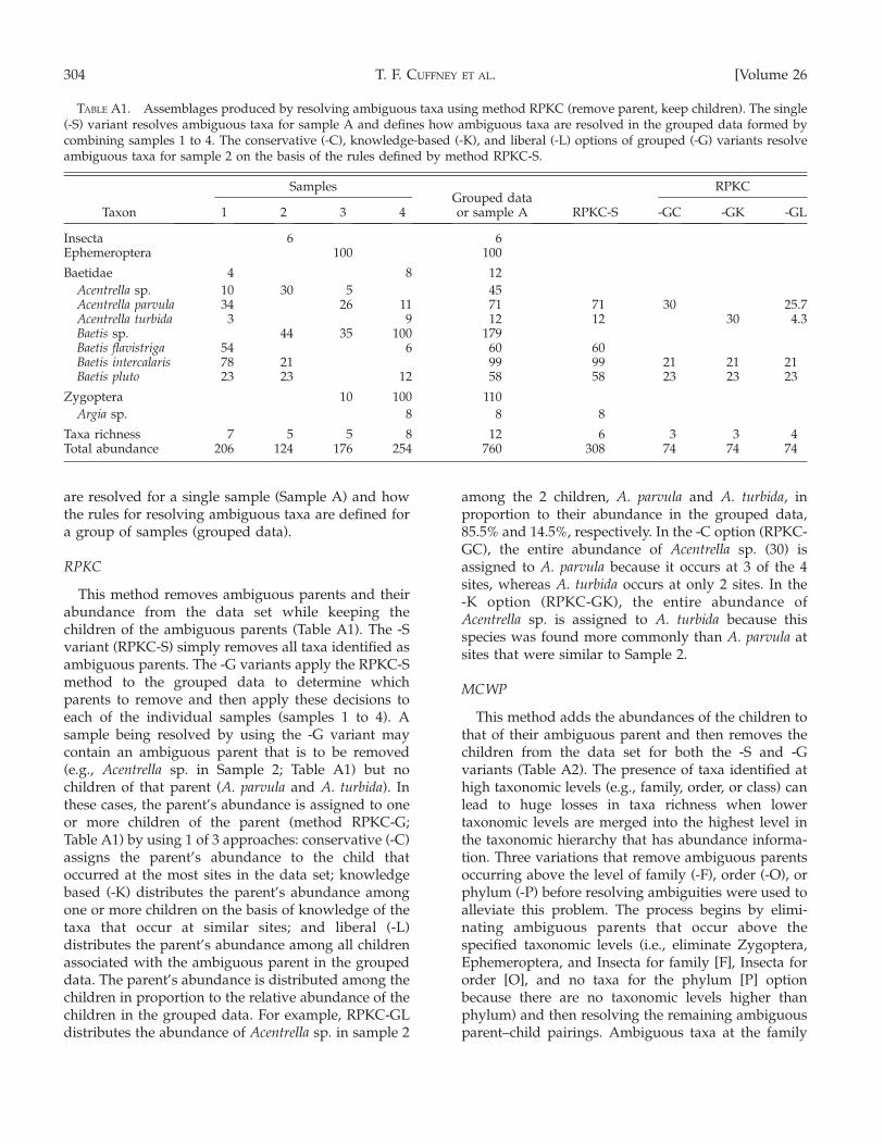
are resolved for a single sample (Sample A) and howthe rules for resolving ambiguous taxa are defined fora group of samples (grouped data).

RPKC

This method removes ambiguous parents and theirabundance from the data set while keeping thechildren of the ambiguous parents (Table A1). The -Svariant (RPKC-S) simply removes all taxa identified asambiguous parents. The -G variants apply the RPKC-Smethod to the grouped data to determine whichparents to remove and then apply these decisions toeach of the individual samples (samples 1 to 4). Asample being resolved by using the -G variant maycontain an ambiguous parent that is to be removed(e.g., Acentrella sp. in Sample 2; Table A1) but nochildren of that parent (A. parvula and A. turbida). Inthese cases, the parent’s abundance is assigned to oneor more children of the parent (method RPKC-G;Table A1) by using 1 of 3 approaches: conservative (-C)assigns the parent’s abundance to the child thatoccurred at the most sites in the data set; knowledgebased (-K) distributes the parent’s abundance amongone or more children on the basis of knowledge of thetaxa that occur at similar sites; and liberal (-L)distributes the parent’s abundance among all childrenassociated with the ambiguous parent in the groupeddata. The parent’s abundance is distributed among thechildren in proportion to the relative abundance of thechildren in the grouped data. For example, RPKC-GLdistributes the abundance of Acentrella sp. in sample 2

among the 2 children, A. parvula and A. turbida, inproportion to their abundance in the grouped data,85.5% and 14.5%, respectively. In the -C option (RPKC-GC), the entire abundance of Acentrella sp. (30) isassigned to A. parvula because it occurs at 3 of the 4sites, whereas A. turbida occurs at only 2 sites. In the-K option (RPKC-GK), the entire abundance ofAcentrella sp. is assigned to A. turbida because thisspecies was found more commonly than A. parvula atsites that were similar to Sample 2.

MCWP

This method adds the abundances of the children tothat of their ambiguous parent and then removes thechildren from the data set for both the -S and -Gvariants (Table A2). The presence of taxa identified athigh taxonomic levels (e.g., family, order, or class) canlead to huge losses in taxa richness when lowertaxonomic levels are merged into the highest level inthe taxonomic hierarchy that has abundance informa-tion. Three variations that remove ambiguous parentsoccurring above the level of family (-F), order (-O), orphylum (-P) before resolving ambiguities were used toalleviate this problem. The process begins by elimi-nating ambiguous parents that occur above thespecified taxonomic levels (i.e., eliminate Zygoptera,Ephemeroptera, and Insecta for family [F], Insecta fororder [O], and no taxa for the phylum [P] optionbecause there are no taxonomic levels higher thanphylum) and then resolving the remaining ambiguousparent–child pairings. Ambiguous taxa at the family

TABLE A1. Assemblages produced by resolving ambiguous taxa using method RPKC (remove parent, keep children). The single(-S) variant resolves ambiguous taxa for sample A and defines how ambiguous taxa are resolved in the grouped data formed bycombining samples 1 to 4. The conservative (-C), knowledge-based (-K), and liberal (-L) options of grouped (-G) variants resolveambiguous taxa for sample 2 on the basis of the rules defined by method RPKC-S.

Taxon

SamplesGrouped dataor sample A RPKC-S

RPKC

1 2 3 4 -GC -GK -GL

Insecta 6 6Ephemeroptera 100 100

Baetidae 4 8 12

Acentrella sp. 10 30 5 45Acentrella parvula 34 26 11 71 71 30 25.7Acentrella turbida 3 9 12 12 30 4.3Baetis sp. 44 35 100 179Baetis flavistriga 54 6 60 60Baetis intercalaris 78 21 99 99 21 21 21Baetis pluto 23 23 12 58 58 23 23 23

Zygoptera 10 100 110

Argia sp. 8 8 8

Taxa richness 7 5 5 8 12 6 3 3 4Total abundance 206 124 176 254 760 308 74 74 74


level (Baetidae) caused abundances to be totaled at thefamily level for method MCWP-SF. Specimens thatcould be identified only to suborder (Zygoptera) andorder (Ephemeroptera) caused all abundances to beadded into Ephemeroptera and Zygoptera aftereliminating data above the order level (i.e., Insecta)for method MCWP-SO. The presence of 6 specimensthat could be identified only to the class level (Insecta)caused all abundance data (760) to be added intoInsecta for method MCWP-SP.

The -G variants of method MCWP (Table A2) applythe appropriate variant of method MCWP-S (-SF, -SO,or -SP) to the grouped data to define the rules forremoving ambiguous parents and merging ambiguousparent–child pairs. For example, MCWP-SF removedthe ambiguous parents Insecta, Ephemeroptera, andZygoptera and merged all mayflies into the familyBaetidae. This results in the removal of the 100 organ-isms that were identified to Ephemeroptera in sample 3,the assignment of 66 organisms (Acentrella sp., A.parvula, Baetis sp.) to Baetidae, even though this samplecontained no organisms identified to this level, and theremoval of 10 organisms identified to Zygoptera. The -Ovariant merged all the mayflies into Ephemeroptera, butkept the 10 organisms identified to Zygoptera. The -Pvariant merged all data into the Insecta.

RPMC

This method resolves ambiguous taxa by applyingeither method RPKC or MCWP to each ambiguousparent–child pair (Table A3). If the collective abun-dance of the children is greater than the abundance of

the ambiguous parent, method RPKC is used; other-wise method MCWP is used. The abundances thatwere eliminated in previous ambiguous parent–childpairings are considered part of the total abundance ofthe children in subsequent pairings. Table A4 illus-trates the application of RPMC-G through 3 iterations.The 1st iteration resolves the genus–tribe pairing byusing method RPKC to eliminate the ambiguousparent Tanytarsini because its abundance (5) is lessthan that of the children (65). The eliminated abun-dance (5) is added to the carry over row for use in thenext pairing (tribe–subfamily). This carry over ensuresthat subsequent comparisons of ambiguous parent–child abundances reflect all the children associatedwith the parent. For example, the tribe–subfamilypairing compares the abundance of the ambiguousparent Chironominae (225) to that of its children (200)and the amount carried over from previous pairings(5). The collective abundance of the children (205) isless than the parent (225) so method MCWP is used tomerge the children with the parent (Chironominae ¼430) and the abundance of Tanytarsini (5) is eliminatedfrom the carry over row because it is now part of theabundance reported for Chironominae. In contrast, theabundance of Diamesinae (10) is less than that of itschildren (100) so Diamesinae is eliminated (RPKC)from the data and added to the carry over row (10) forconsideration in the subfamily–family pairing. In thefinal pairing (subfamily–family), the abundance of theambiguous parent Chironomidae (100) is less than thecombined abundance of the children (530) and thecarry over (10), so the abundance of the parent is

TABLE A2. Assemblages produced by resolving ambiguous taxa using method MCWP (merge children with parents). The family(-F), order (-O), and phylum (-P) single (-S) variants resolve ambiguous taxa for sample A and define how ambiguous taxa areresolved in the grouped data formed by combining samples 1 to 4. The grouped (-G) variants resolve ambiguous taxa for sample 3on the basis of the rules defined by the corresponding variant of method RPKC-S.

Taxon

SampleGrouped dataor Sample A

MCWP

1 2 3 4 -SF -SO -SP -GF -GO -GP

Insecta 6 6 760 176Ephemeroptera 100 100 636 166

Baetidae 4 8 12 536 66

Acentrella sp. 10 30 5 45Acentrella parvula 34 26 11 71Acentrella turbida 3 9 12Baetis sp. 44 35 100 179Baetis flavistriga 54 6 60Baetis intercalaris 78 21 99Baetis pluto 23 23 12 58

Zygoptera 10 100 110 118 10

Argia sp. 8 8 8

Taxa richness 7 5 5 8 12 2 2 1 1 2 1Total abundance 206 124 176 254 760 544 754 760 66 176 176


eliminated (RPKC) from the data set and added to thecarry over value, which becomes 110 and would beconsidered in the next parent–child pairing (family–order).

The rules used for the -G variant (RPMC-G) arederived by applying RPMC-S (Table A3) to the

grouped data. When these rules are applied to sample3, the Ephemeroptera, Acentrella sp., and Baetis sp. areremoved from the sample even though the combinedabundance of the children of Ephemeroptera insample 3 (100) is greater than the children (66). Thisremoval occurs because the abundance of the Ephem-

TABLE A3. Assemblages produced by resolving ambiguous taxa using methods RPMC (remove parent or merge children withparent) and DPAC (distribute parent among children). The single (-S) variants resolve ambiguous taxa for sample A and define howambiguous taxa are resolved in the grouped data formed by combining samples 1 to 4. The conservative (-C), knowledge-based(-K), and liberal (-L) options of grouped (-G) variants resolve ambiguous taxa for sample A on the basis of the rules defined by themethod RPMC-S or DPAC-S.

SamplesGrouped dataor Sample A

RPMC DPAC

Taxon 1 2 3 4 -S -G -S -GC -GK -GL

Insecta 6 6Ephemeroptera 100 100

Baetidae 4 8 12

Acentrella sp. 10 30 5 45Acentrella parvula 34 26 11 71 71 26 134.0 78.0 78.0 78.0Acentrella turbida 3 9 12 12 22.6Baetis sp. 44 35 100 179Baetis flavistriga 54 6 60 60 134.0 24.3Baetis intercalaris 78 21 99 99 221.0 88.0 40.2Baetis pluto 23 23 12 58 58 129.5 88.0 23.5

Zygoptera 10 100 110 118 10

Argia sp. 8 8 118.9 10.0 10.0 10.0

Taxa richness 7 5 5 8 12 6 5 6 3 3 5Total abundance 206 124 176 254 760 418 192 760 176 176 176

TABLE A4. An example of iteratively resolution of ambiguous parent–child pairs in a progression from genus to family using thegrouped (-G) option of method RPMC (remove parent or merge children). This method considers the abundance of organisms thathave been removed in previous iterations (carry over) when comparing ambiguous parent–child abundances in subsequentiterations.

Iteration 1 Iteration 2 Iteration 3Taxonomic level

Originalabundance

Genus–tribe

Tribe–subfamily

Subfamily–familyFamily Subfamily Tribe Genus

Chironomidae 100 100 100 0Chironominae 225 225 430 430

Chironomini 100 135 0 0Chernoushii 10 0 0 0Chironomus 20 0 0 0Cladopelma 5 0 0 0

Tanytarsini 5 0 0 0Cladotanytarsus 15 15 0 0Microspectra 20 20 0 0Neozaurelia 30 30 0 0

Diamesinae 10 10 0 0Diamesa 15 15 15 15Pagastia 35 35 35 35Potthastia 50 50 50 50

Total resolved 640 635 630 530Carry over 0 5 10 110Total processed 640 640 640 640


eroptera in the grouped data (100) is much less thanthat of the children (536) so Ephemeroptera is deletedfrom the grouped data and all samples. Baetis sp. isremoved for the same reason even though it is moreabundant (35) in sample 3 than are the children (0).The removal of Acentrella sp. and the retention ofZygoptera also occur by the rules identified for thegrouped data.

DPAC

This method distributes the abundance of theambiguous parent among the children in proportionto the relative abundance of each child in the sample(Table A3). If more than one child is associated withthe ambiguous parent, the parent’s abundance isdivided among the children in proportion to therelative abundance of each child. Table A5 illustrateshow abundances of parents are distributed amongtheir children for method DPAC-S (Table A3). The firstambiguous parent–child pairs occur at the genus–species level (Table A5) where the abundances of theambiguous parents (Acentrella sp. and Baetis sp.) aredivided among their respective children in proportionto the abundance of the children (e.g., 85.5% ofAcentrella sp. is added to A. parvula and 14.5% isadded to A. turbida). The next ambiguous parent–child

pairings occur at the family–genus level where the

abundance of Baetidae (12) is divided among the

species of Acentrella and Baetis on the basis of their

relative abundances after resolving ambiguous parents

at the genus level (e.g., 20.9% would be assigned to A.parvula). Taxa richness decreases with each iteration,

but the total abundance remains the same.

Use of method DPAC to resolve ambiguous taxa for

a group of samples (DPAC-G) can lead to situations

where the rules developed for the grouped data

(DPAC-S; Table A3) call for dividing an ambiguous

parent among its children, but none of the children are

present in the sample (e.g., sample 2 in Table A3

contains the ambiguous parent Acentrella sp., but

neither of the children, A. parvula and A. turbida). In

these situations, we have elected to use the same

approach as previously used for method RPKC-G. We

pick the children over which the parent’s abundance

will be distributed on the basis of the children in the

grouped data. This process generates new taxa that

were not in the original sample (OTUs). The -C, -K,

and -L approaches are the same as used for RPKC-G.

The abundance of the ambiguous parent is distributed

among the children in accordance with their relative

abundance in the grouped data (Table A3).

TABLE A5. An example of how the single (-S) variant of method DPAC (distribute parents among children) resolves ambiguoustaxa in the original data (ORIG) starting with ambiguous parent–children pairs at the genus–species level and progressing to theclass–order level. This method distributes the abundance of the ambiguous parents (p) among the children in accordance with therelative abundance of each child. The relative abundance of each child is determined on the basis of the distribution of abundancesthat occurred in the previous level. Boldface type indicates the abundances that were modified by the distribution of parent’sabundances in each iteration from genus to class.

Taxon ORIG

Ambiguous parent

Genus Family Suborder Order Class

Insecta (p) 6 6 6 6 6Ephemeroptera (p) 100 100 100 100

Baetidae (p) 12 12

Acentrella sp. (p) 45A. parvula 71 109.5 112.0 112.0 132.9 134.0A. turbida 12 18.5 18.9 18.9 22.5 22.6Baetis sp. (p) 179B. flavistriga 60 109.5 112.0 112.0 132.9 134.0B. inercalaris 99 180.7 184.8 184.8 219.3 221.0B. pluto 58 105.8 108.3 108.3 128.5 129.5

Zygoptera (p) 110 110 110

Argia sp. 8 8 8 118.0 118.0 118.9

Taxa richness 12 10 9 8 7 6Total abundance 760 760 760 760 760 760


Documents

Ambiguous taxa: effects on the characterization and ... · 2007 by The North American Benthological Society ... The choice of method used to ... or distribute taxa) that are commonly