Embed Size (px)
Citation preview

Ambiguous Business Cycles∗
Cosmin IlutDuke University
Martin SchneiderStanford University
April 2011
Abstract
This paper considers business cycle models with agents who are averse not only torisk, but also to ambiguity (Knightian uncertainty). Ambiguity aversion is describedby recursive multiple priors preferences that capture agents’ lack of confidence inprobability assessments. While modeling changes in risk typically calls for higher orderapproximations, changes in ambiguity in our models work like changes in conditionalmeans. Our models thus allow for uncertainty shocks but can still be solved andestimated using simple 1st order approximations. In an otherwise standard businesscycle model, an increase in ambiguity (that is, a loss of confidence in probabilityassessments), acts like an ’unrealized’ news shock: it generates a large recessionaccompanied by ex-post positive excess returns.
1 Introduction
Recent events have generated renewed interest in the effects of changing uncertainty on
macroeconomic aggregates. The standard framework of quantitative macroeconomics is
based on expected utility preferences and rational expectations. Changes in uncertainty
are typically modeled as expected and realized changes in risk. Indeed, expected utility
agents think about the uncertain future in terms of probabilities. An increase in uncertainty
is described by the expected increase in a measure of risk (for example, the conditional
volatility of a shock or the probability of a disaster). Moreover, rational expectations implies
that agents’ beliefs coincide with those of the econometrician (or model builder). An expected
increase in risk must on average be followed by a realized increase in the volatility of shocks
or the likelihood of disasters.
This paper studies business cycle models with agents who are averse to ambiguity
(Knightian uncertainty). Ambiguity averse agents do not think in terms of probabilities
∗Preliminary and incomplete.
1
– they lack the confidence to assign probabilities to all relevant events. An increase in
uncertainty may then correspond to a loss of confidence that makes it more difficult to
assign probabilities. Formally, we describe preferences using multiple priors utility (Gilboa
and Schmeidler (1989)). Agents act as if they evaluate plans using a worst case probability
drawn from a set of multiple beliefs. A loss of confidence is captured by an increase in the set
of beliefs. It could be triggered, for example, by worrisome news about the future. Agents
respond to a loss of confidence as their worst case probability changes.
The paper proposes a simple and tractable way to incorporate ambiguity and shocks to
confidence into a business cycle model. Agents’ set of beliefs is parametrized by an interval
of means for exogenous shocks, such as innovations to productivity. A loss of confidence is
captured by an increase in the width of such an interval; in particular it makes the “worst
case” mean even worse. Intuitively, a shock to confidence thus works like a news shock: an
agent who loses confidence responds as if he had received bad news about the future. The
difference between a loss of confidence and bad news is that the latter is followed, on average,
by the realization of a bad outcome. This is not the case for a confidence shock.
We study ambiguity and confidence shocks in economies that are essentially linear. The
key property is that the worst case means supporting agents’ equilibrium choices can be
written as a linear function of the state variables. It implies that equilibria can be accurately
characterized using first order approximations. In particular, we can study agents’ responses
to changes in uncertainty, as well as time variation in uncertainty premia on assets, without
resorting to higher order approximations. This is in sharp contrast to the case of changes in
risk, where higher order solutions are critical. We illustrate the tractability of our method
by estimating a medium scale DSGE model with ambiguity about productivity shocks.
The effects of a lack of confidence are intuitive. On average, less confident agents engage
in precautionary savings and, other things equal, accumulate more steady state capital.
A sudden loss of confidence about productivity generates a wealth effect – due to more
uncertain wage and capital income in the future, and also a substitution effect since the
return on capital has become more uncertain. The net effect on macroeconomic aggregates
depends on the details of the economy. In our estimated medium scale DSGE model, a
loss of confidence generates a recession in which consumption, investment and hours decline
together. In addition, a loss of confidence generates increased demand for safe assets, and
opens up a spread between the returns on ambiguous assets (such as capital) and safe assets.
Business cycles driven by changes in confidence thus give rise to countercyclical spreads or
premia on uncertain assets.
Our paper is related to several strands of literature. The decision theoretic literature on
ambiguity aversion is motivated by the Ellsberg Paradox. Ellsberg’s experiments suggest
2

that decision makers’ actions depend on their confidence in probability assessments – they
treat lotteries with known odds differently from bets with unknown odds. The multiple
priors model describe such behavior as a rational response to a lack of information about
the odds. To model intertemporal decision making by agents in a business cycle model, we
use a recursive version of the multiple priors model that was proposed by Epstein and Wang
(1994) and has recently been applied in finance (see Epstein and Schneider (2010) for a
discussion and a comparison to other models of ambiguity aversion). Axiomatic foundations
for recursive multiple priors were provided by Epstein and Schneider (2003).
Hansen et al. (1999) and Cagetti et al. (2002) study business cycles models with robust
control preferences. Under the robust control approach, preferences are smooth – utility
contains a smooth penalty function for deviations of beliefs from some reference belief.
Smoothness rules out first order effects of uncertainty. Models of changes in uncertainty
with robust control thus rely on higher order approximations, as do models with expected
utility. In contrast, multiple priors utility is not smooth when belief sets differ in means.
As a result, there are first order effects of uncertainty – this is exactly what our approach
exploits to generate linear dynamics in response to uncertainty shocks.
The mechanics of our model are related to the literature on news shocks (for example
Beaudry and Portier (2006), Christiano et al. (2008), Schmitt-Grohe and Uribe (2008),
Jaimovich and Rebelo (2009),Christiano et al. (2010a) and Barsky and Sims (2011)). In
particular, Christiano et al. (2008) have considered the response to temporary unrealized
good news about productivity to study stock market booms. When we apply our approach
to news about productivity, a loss confidence works like a (possibly persistent) unrealized
decline in productivity. Recent work on changes in uncertainty in business cycle models has
focused on changes in realized risk – looking either at stochastic volatility of aggregate shocks
(see for example Fernandez-Villaverde and Rubio-Ramirez (2007), Justiniano and Primiceri
(2008), Fernandez-Villaverde et al. (2010) and the review in Fernandez-Villaverde and Rubio-
Ramırez (2010)) or at changes in idiosyncratic volatility in models with heterogeneous firms
(Bloom et al. (2009), Bachmann et al. (2010)). We view our work as complementary to
these approaches. In particular, confidence shocks can generate responses to uncertainty –
triggered by news, for example – that is not connected to later realized changes in risk.
The paper proceeds as follows. Section 2 presents a general framework for adapting
business cycle models to incorporate ambiguity aversion. Section 3 discusses the applicability
of linear methods. Section 4 describes the estimation of a DSGE model for the US.
3

2 Ambiguous business cycles: a general framework
Uncertainty is represented by a period state space S. One element s ∈ S is realized every
period, and the history of states up to date t is denote st = (s0, ..., st).
Preferences
Preferences order uncertain streams of consumption C = (Ct)∞t=0, where Ct : St → <n and
n is the number of goods. Utility for a consumption process C = {Ct} is defined recursively
by
Ut(C; st
)= u (Ct) + β min
p∈P(st)Ep [Ut+1 (C; st, st+1)] , (2.1)
where P (st) is a set of probabilities on S.
Utility after history st is given by felicity from current consumption plus expected
continuation utility evaluated under a “worst case” belief. The worst case belief is drawn
from a set Pt (st) that may depend on the history st. The primitives of the model are the
felicity u, the discount factor β and the entire process of one-step-ahead belief sets Pt (st).
Expected utility obtains as a special case if all sets Pt (st) contain only one belief. More
generally, a nondegenerate set of beliefs captures the agent’s lack of confidence in probability
assessments; a larger set describes a less confident agent.
For our applications, we assume Markovian dynamics. In particular, we restrict belief sets
to depend only on the last state and write Pt (st). We also assume that the true law of motion
– from the perspective of an observer – is given by a transition probability p∗ (st) ∈ Pt (st).
The assumption here is that agents know that the dynamics are Markov, but they are not
confident in what transition probabilities to assign. However, they are not systematically
wrong in the sense that they view the true transition possibility as impossible. The true
DGP is not relevant for decision making, but it matters for characterizing the equilibrium
dynamics.
Environment & equilibrium
We consider economies with many agents i ∈ I. Agent i’s preferences are of the form
(2.1) with primitives (βi, ui, {P it (st)}). Given preferences, it is helpful to write the rest of the
economy in fairly general notation that many typical problems can be mapped into. Consider
a recursive competitive equilibrium that is described using a vector X of endogenous state
variables. Let Ai denote a vector of actions taken by agent i. Among those actions is the
choice of consumption – we write ci (Ai) for agent i′s consumption bundle implied when the
action is Ai. Finally, let Y denote a vector of endogenous variables not chosen by the agent
– this vector will typically include prices, but also variables such as government transfers
that are endogenous, but are neither part of the state space nor actions or prices.
4

The technology and market structure are summarized by a set of reduced form functions
or correspondences. A recursive competitive equilibrium consists of action and value
functions Ai and V i, respectively, for all agents i ∈ I, as well as a function describing
the other endogenous variables Y . We also write A for the collection of all actions (Ai)i∈Iand A−i for the collection of all actions except that of agent i. All functions are defined on
the state (X, s) and satisfy
W i (A,X, s; p) = ui(ci(Ai))
+ βiEp[V i(x′ (X,A, Y (X, s) , s, s′) , s′)
];i ∈ I (2.2)
Ai (X, s) = arg maxAi∈Bi(Y (X,s),A−i,X,s)
minp∈Pi(s)
W (A,X, s; p) i ∈ I (2.3)
V i (X, s) = minp∈Pi(s)
W i (A (X, s) , X, s; p) (2.4)
0 = G (A(X, s), Y (X, s) , X, s) (2.5)
The first equation simply defines the agent’s objective in state (X, s) , while the second
and third equation provide the optimal policy and value. Here Bi is the agent’s budget set
correspondence and the function x′ describes the transition of the endogenous state variables.
The function G summarizes all other contemporaneous relationships such as market clearing
or the government budget constraint – there are enough equations in (2.5) to determine the
endogenous variables Y .
Characterizing optimal actions & equilibrium dynamics
For every state (X, s), there is a measure p0i (X, s) that achieves the minimum for agent
i in (2.3). Since the minimization problem is linear in probabilities, we can replace P it by
its convex hull without changing the solution. The minimax theorem then implies that
we can exchange the order of minimization and maximization in the problem (2.3). It
follows that the optimal action Ai is the same as the optimal action if the agent held the
probabilistic belief p0i (X, s) to begin with. In other words, for every equilibrium of our
economy, there exists an economy with expected utility agents holding beliefs p0i that has
the same equilibrium.
The observational equivalence just described suggests the following guess-and-verify
procedure to compute an equilibrium wtih ambiguity aversion:
1. guess the worst case beliefs p0i
2. solve the model assuming that the agents have expected utility and beliefs p0i
3. compute the value functions V i
4. verify that the guesses p0i indeed achieves the minimum in (2.4) for every i.
5

Suppose we have found the optimal action functions A as well as the response of the
endogenous variables Y and hence the transition for the states X. We are interested in
stochastic properties of the equilibrium dynamics that can be compared to the data. We
characterize the dynamics in the standard way by calculating (for example or simulating)
moments of the economy under the true distribution of the exogenous shocks p∗. The only
unusual feature is that this true distribution need not coincide with the distribution p0i that
is used to compute optimal actions.
Shocks to confidence
We now specialize a process of belief sets Pt to capture random changes in confidence. For
simplicity, assume that there is a single exogenous process z that directly affects the economy,
for example productivity or a monetary policy shock. In additon to z, the exogenous state
s has a second component vt that captures time variation in confidence. Suppose the true
dynamics of exogenous state s can be represented by an AR(1) process
zt+1 = ρzzt + εzt+1,
vt+1 = (1− ρv) v + ρvvt + εvt+1
where the shocks εz and εv are iid and normally distributed shock with mean zero and
variances σ2z and σ2
v , respectively.
The component vt is a tool to describe the evolution of the belief set Pt. In particular,
we assume that the agent knows the evolution of vt, but that he is not sure whether the
conditional mean of zt+1 is really ρzzt. Instead, he allows for a range of intercepts. The set
Pt can thus be represented by the family of processes
zt+1 = ρzzt + at + εzt+1,
at ∈ [−vt,−vt + 2|vt|]
vt+1 = (1− ρv) v + ρvvt + εvt+1 (2.6)
If vt is higher, then the agent is less confident about the mean.of zt+1 – his belief set is larger.
The worst case belief p0 is now described by a worst case intercept v0t . Changes in ambiguity
parametrized by vt change the worst case conditional mean ρzzt + v0t and therefore have 1st
order effects on behavior.
As long as vt > 0, the interval of intercepts contemplated by the agent is centered around
zero – it can equivalently be described by the condition at ≤ |vt|. In contrast, if vt becomes
negative, then all intercepts are positive - the agent is thus optimistic relative to the truth.
In applications, it is thus useful to parametrize the dynamics such that v does not become
6

negative very often. The advantage of the present parametrization is that the lower bound,
which plays a special role in the computation, is guaranteed to have linear dynamics.
3 Computation in essentially linear economies
The computation and interpretation of equilibria is particularly simple if all dynamics is
approximately linear. We start from the assumption that the environment (given by Bi,
x′ ui and G) is such that, under expected utility and rational expectations, a first order
solution provides a satisfactory approximation to the equilibrium dynamics. Under rational
expectations, the innovations to vt are news shocks that provide information about zt
one period ahead. In many applications, standard tools will reveal whether a first order
approximation is satisfactory.
It is now natural to look for an equilibrium such that the worst case intercepts v0it are all
linear in the state variables. If such an equilibrium exists, we call the economy essentially
linear. In an essentially linear economy, the choices A and other endogenous variables Y will
all be well approximated by linear functions of the state variables. The equilibrium dynamics
is thus described by a linear state space system with all shocks – including uncertainty
shocks – driven by the (true) linear laws of motion. In many interesting economies, it is
straightforward to establish essential linearity. Consider, for example, a baseline stochastic
growth model with a representative agent who perceives ambiguity about productivity. The
worst case is that the mean of productivity innovations is always as low as possible, so
v0t = −vt.
More generally, to check whether some general economy is essentially linear, we specialize
the guess-and-verify procedure described above. Step 2 of the procedure consists of solving
the model using the guesses p0i that sets v0it = −vt or v0i
t = vt. In other words, the worst case
for agent i is always either the highest or lowest bound of the interval. Since these guesses
just implies a linear shift of the shock, this step can also be done by first order methods.
In particular, we propose to linearize the model around a “zero risk” steady state that sets
the variance of the shocks to a very small number while retaining the effect of ambiguity on
decisions. Properties of zero risk steady states are described in more detail below.
To implement step 3 of the procedure, let V 0i denote the value function for the problem
with expected utility and at at the guessed worst case mean for agent i in (2.6). For example,
consider an agent with v0it = −vt. For this agent, we verify the guess by checking whether
for any X,A, s = (z, v) and v′, the function
V (z′) := V 0(x′ (X,A, Y (X, s) , s, z′, v′) , z′, v′)
7

is strictly increasing. We do the opposite check for an agent with v0it = vt.. At this stage,
nonlinearity of the value function could be important. We thus compute the value function
using higher order approximations and form the function V accordingly.
In what follows, we first describe the dynamics and then the calculation of the zero risk
steady state.
3.1 Dynamics
Let xt denote the endogenous variables of interest. Posit a linear equilibrium law of motion:
xt = Axt−1 +Bst,
where st are the exogenous variables. For notational purposes, split the vector st into the
technology shock zt ≡ log zt, mean distortion (or news) vt and the rest of the exogenous
variables, s∗t .
Posit another linear relation for the exogenous variables:
st =
s∗t
zt
vt
= P
s∗t−1
zt−1
vt−1
+
εt
εzt
εvt
Ξt =
εt
εzt
εvt
∼ N (0,Σ)
Ξt denotes the innovations to the exogenous variables st. They are defined to be zero mean.
We follow the method of undetermined coefficients of Christiano (2002) to solving
a system of linear equations with rational expectations. Let the linearized equilibrium
conditions be restated in general as:
Et[α0xt+1 + α1xt + α2xt−1 + β0st+1 + β1st] = 0 (3.1)
where α0, α1, α2, β0, β1 are constants determined by the equilibrium conditions. Importantly
8

for us,
Et
s∗t+1
zt+1
vt+1
= P
s∗t
zt
vt
+ Et
εt+1
εzt+1
εvt+1
Et
εt+1
εzt+1
εvt+1
= 0
To reflect the time t information (news, or mean distortion) about zt+1 we remember that
Etzt+1 = ρz zt − vt
so the matrix P satisfies the restriction:
P =
ρ 0 0
0 ρz −1
0 0 ρv
Et
s∗t+1
zt+1
vt+1
=
ρ 0 0
0 ρz −1
0 0 ρv
s∗t
zt
vt
+ Et
εt+1
εzt+1
εvt+1
where ρ is a diagonal matrix reflecting the autocorrelation structure of the elements in
s∗t .Notice that without the ”news” part, the standard form for P is:
P =
ρ 0 0
0 ρz 0
0 0 ρv
Substitute the posited policy rule into linearized equilibrium conditions:
0 = Et[α0(Axt +Bst+1) + α1 (Axt−1 +Bst) + α2xt−1 + β0 (Pst + Ξt+1) + β1st]
to get:
0 =(α0A
2 + α1A+ α2
)xt−1 + (α0AB + α0BP + α1B + β0P + β1) st + (α0B + β0)EtΞt+1
0 = EtΞt+1
9

Thus, A is the matrix eigenvalue of matrix polynomial:
α(A) = α0A2 + α1A+ α2 = 0
and B satisfies the system of linear equations:
F = (β0 + α0B)P + [β1 + (α0A+ α1)B] = 0
The solution to the model obtained so far is one in which the mean distortion vt to the
process for zt+1 is realized.
With this solution in hand, look at the variables when the negative mean distortion is
not realized at each period t. In the equilibrium defined above:
xt = Axt−1 +Bst (3.2)
st =
s∗t
zt
vt
=
ρ 0 0
0 ρz −1
0 0 ρv
s∗t−1
zt−1
vt−1
+ Ξt
but now we have:
xt = Axt−1 +Bst
st =
s∗t
zt
vt
=
ρ 0 0
0 ρz 0
0 0 ρv
s∗t−1
zt−1
vt−1
+
εt
εzt
εvt
st =
ρ 0 0
0 ρz −1
0 0 ρv
s∗t−1
zt−1
vt−1
+
0 0 0
0 0 1
0 0 0
s∗t−1
zt−1
vt−1
+ Ξt
st = P
s∗t−1
zt−1
vt−1
+ C
s∗t−1
zt−1
vt−1
+ Ξt, C ≡
0 0 0
0 0 1
0 0 0
so:
xt = Axt−1 +Bst
xt = Axt−1 +BP
s∗t−1
zt−1
vt−1
+B
0 0 0
0 0 1
0 0 0
s∗t−1
zt−1
vt−1
+BΞt
10

or in other words, for every j element in the vector xt, where the superscript j refers to the
jth row of the corresponding matrix, we have:
xjt = Ajxt−1 +BjPst−1 +BjΞt +Bjzvt−1 (3.3)
where the element Bjz refers to the coefficient of the matrix B that reflects the response of
the element xjt to the realized state zt.
Notice that the evolution in (3.3) defines the equilibrium law of motion for our economy.
From the perspective of the economy in (3.2) it is interpreted as the response to an ”unusual”
innovation to εzt whose value is not zero (on average) but rather vt−1. However, conditional
on this ”innovation” (state of the economy xt) the expectations are still governed by the
equation (3.1) where for example the expectation about zt+1 is:
Etzt+1 = ρz zt − vt
3.1.1 Zero risk steady state
We now describe an approach to find the stochastic steady state of our model using the
linearized law of motion of the endogenous variables. Take the perceived law of motion:
zt+1 = ρz zt + σεzt+1 − v
where v is the steady state level of vt. We can summarize our procedure in the following
steps:
1. Find the deterministic ’distorted’ steady state in which the intercept is actually −v.
The steady state technology level is then
zo = exp
(−v
1− ρz
)Using zo, one can compute the deterministic ’distorted’ steady state, by analyzing the FOC
of these economy. Denote these steady state values of the m variables as a vector xo
xom×1
2. Linearize the model around this deterministic ’distorted’ steady state.
For example, in the above notations, looks for matrices A,B that describe the evolution
11
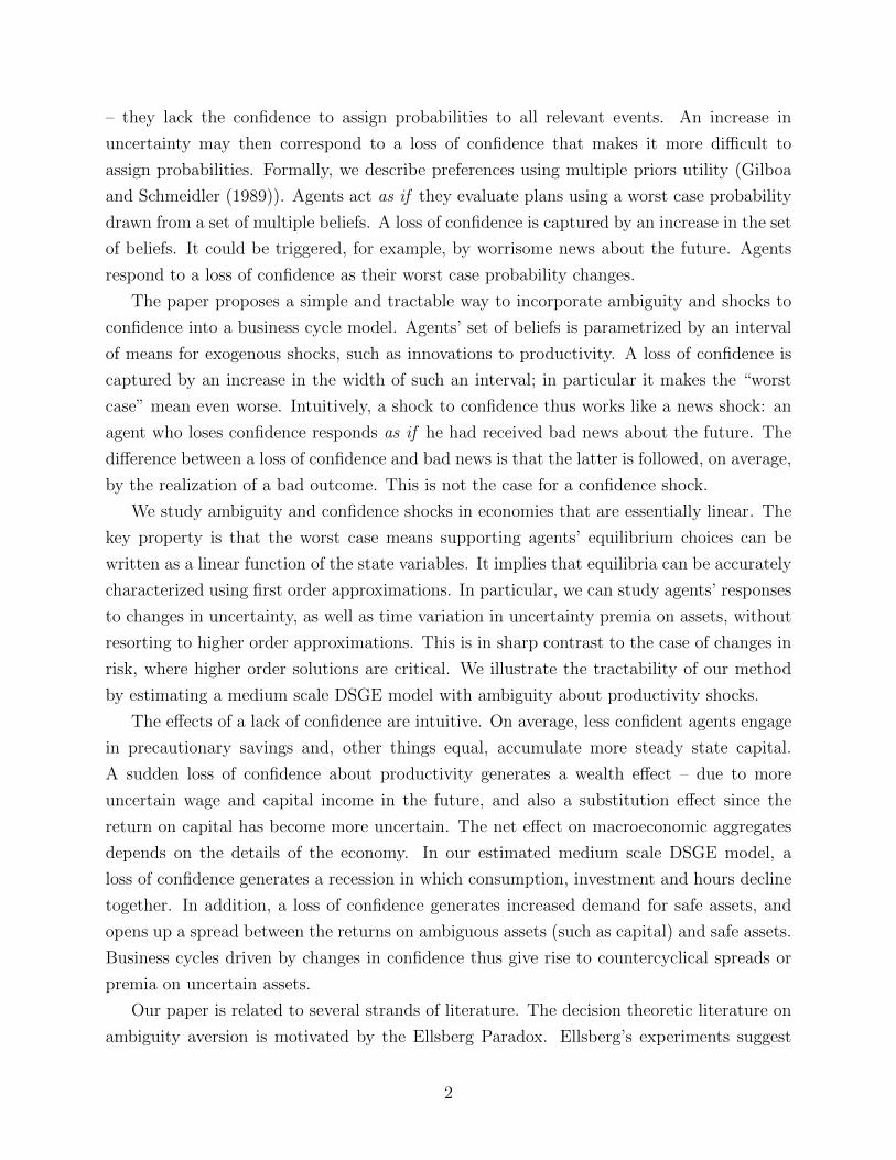
of the variables as:
xt − xo = A(xt−1 − xo) +BP (st−1 − so) +B(Ξt − Ξo) (3.4)
st =
s∗t
zt
vt
=
ρ 0 0
0 ρz −1
0 0 ρv
s∗t−1
zt−1
vt−1
+ Ξt
where Ξt are the innovations to the stochastic shock processes. Let the size of this vector be
n× 1, where the first element refers to the innovation of the technology shock.
Notice for example that when innovations are equal to their expected values, set to zero,
i.e. that Ξo = 0n×1 and st−1 = so, the law of motion recovers that xt = xo.
So, in step 2 we need to find the matrices A and B. This is done by standard solution
techniques of forward looking rational expectations model.
3. Correct for the fact that, from the perspective of the agent’s ex-ante beliefs, the average
innovation of the technology shock at time t is not equal to 0. The average innovation is
equal to v/σ. Indeed:
Et−1zt = ρz zt−1 − v
but the realized average log zt is
zt = ρz zt−1
Thus, from the perspective of the time t− 1 expectation:
zt = Et−1zt + σεt
εt = v/σ
So, take the law of motion in (3.4) and impose that the first element of Ξt is equal to v/σ,
while keeping the rest equal to 0 :
Ξ =
[v/σ
0(n−1)×1
]
4. Find the steady state of the variables xt, given that the law of motion is:
xt − xo = A(xt−1 − xo) +BP (st−1 − so) +B(Ξt − Ξo)
The steady state version for the exogenous variables is:
sSS − so = P (sSS − so) + (Ξ− Ξo)
12

where sSS are the steady state values of the exogenous variables under their true DGP. So:
sSS = so +
[v/σ
0(n−1)×1
](I − P )−1
Then solve for the rest of the endogenous variables by using:
xSS − xo = A(xSS − xo) +B(sSS − so)
where xSS are the steady state values of the variables under ambiguity. So, xSS can be found
as:
xSS = xo +B(sSS − so) (I − A)−1
4 An estimated model with ambiguity
This section describes the model that we use to describe the US business cycles. The model
is based on a standard medium scale DSGE model along the lines of Christiano et al. (2005)
and Smets and Wouters (2007). The key difference in our model is that decision makers are
ambiguity-averse. We now describe the model structure and the shocks.
4.1 The model
4.1.1 The goods sector
The final output in this economy is produced by a representative final good firm that
combines a continuum of intermediate goods Yj,t in the unit interval by using the following
linear homogeneous technology:
Yt =
[∫ 1
0
Yj,t1
λf,t dj
]λf,t,
where λf,t is the markup of price over marginal cost for intermediate goods firms. The
markup shock evolves as:
log(λf,t/λf ) = ρλf log(λf,t−1/λf ) + λxf,t,
13

where λxf,t is i.i.d.N(0, σ2λf
). Profit maximization and the zero profit condition leads to to
the following demand function for good j:
Yj,t = Yt
(PtPj,t
) λf,tλf,t−1
(4.1)
The price of final goods is:
Pt =
[∫ 1
0
P1
1−λf,tj,t dj
](1−λf,t)
.
The intermediate good j is produced by a price-setting monopolist using the following
production function:
Yj,t = max{εtKαj,t (ztLj,t)
1−α − Φz∗t , 0},
where Φ is a fixed cost and Kj,t and Lj,t denote the services of capital and homogeneous
labor employed by firm j. Φ is chosen so that steady state profits are equal to zero. The
intermediate goods firms are competive in factor markets, where they confront a rental rate,
Ptrkt , on capital services and a wage rate, Wt, on labor services.
The variable, zt, is a shock to technology, which has a covariance stationary growth rate.
The variable, εt, is a stationary shock to technology. The fixed costs are modeled as growing
with the exogenous variable, z∗t :
z∗t = ztΥ( α
1−α t)
with Υ > 1. If fixed costs were not growing, then they would eventually become irrelevant.
We specify that they grow at the same rate as z∗t , which is the rate at which equilibrium
output grows. Note that the growth of z∗t , i.e. µ∗z,t ≡ ∆ log(z∗t ), exceeds that of zt, i.e.
µz,t ≡ ∆ log(zt) :
µ∗z,t = µz,tΥα
1−α .
This is because we have another source of growth in this economy, in addition to the
upward drift in zt. In particular, we posit a trend increase in the efficiency of investment. We
discuss this process as well as the time series representation for the the transitory technology
shock further below. The process for the stochastic growth rate is:
log(µ∗z,t) = (1− ρµ∗z) log µ∗z + ρµ∗z log µ∗z,t−1 + µx∗z,t,
where µx∗z,t is i.i.d.N(0, σ2µ∗z
).
We now describe the intermediate good firms pricing opportunities. Following Calvo
(1983), a fraction 1− ξp, randomly chosen, of these firms are permitted to reoptimize their
price every period. The other fraction ξp cannot reoptimize. Of these, a (randomly selected)
14

fraction (1− ιP ) must set Pit = πPi,t−1 and a fraction ιP set Pit = πt−1Pi,t−1, where π is
steady state inflation. The jth firm that has the opportunity to reoptimize its price does so
to maximize the expected present discounted value of the future profits:
Ep0
t
∞∑s=0
(βξp)s λt+sλt
[Pj,t+sYj,t+s −Wt+sLj,t+s − Pt+srkt+sKj,t+s
], (4.2)
subject to the demand function (4.1), where λt is the marginal utility of nominal income for
the representative household that owns the firm.
It should be noted that the expectation operator in these equations is, in the notation of
the general representation in section 2, the expectation under the worst-case belief p0. This
is because state prices in the economy reflect ambiguity. We will describe the household’s
problem further below.
We now describe the problem of the perfectly competitive ”employment agencies”. The
households specialized labor inputs are aggregated by these agencies into a homogeneous
labor service according to the following function:
Lt =
[∫ 1
0
(li,t)1λw di
]λw.
These employment agencies rent the homogeneous labor service Lt to the intermediate goods
firms at the wage rate Wt. In turn, these agencies pay the wage Wi,t to the household
supplying labor of type i. Similarly as for the final goods producers, the profit maximization
and the zero profit condition leads to to the following demand function for labor input of
type i:
li,t = Lt
(Wt
Wi,t
) λwλw−1
, (4.3)
We follow Erceg et al. (2000) and assume that the household is a monopolist in the supply
of labor by providing li,t and it sets its nominal wage rate, Wi,t. It does so optimally with
probability 1 − ξw and with probability ξw is does not reoptimize its wage. In case it does
not reoptimize, it sets the wage as:
Wi,t = πιwt−1π1−ιwµz∗Wi,t−1,
where µz∗ is the steady state growth rate of the economy. When household i has the chance
to reoptimize, it does do by maximizing the expected present discounted value of future net
15
utility gains of working:
Ep0
t
∞∑s=0t
∞∑s=0
(βξw)s[λt+sWi,t+sli,t+s − ζc,t+sζL,t+s
ψL1 + σL
l1+σLi,t+s
]. (4.4)
subject to the demand function (4.3).
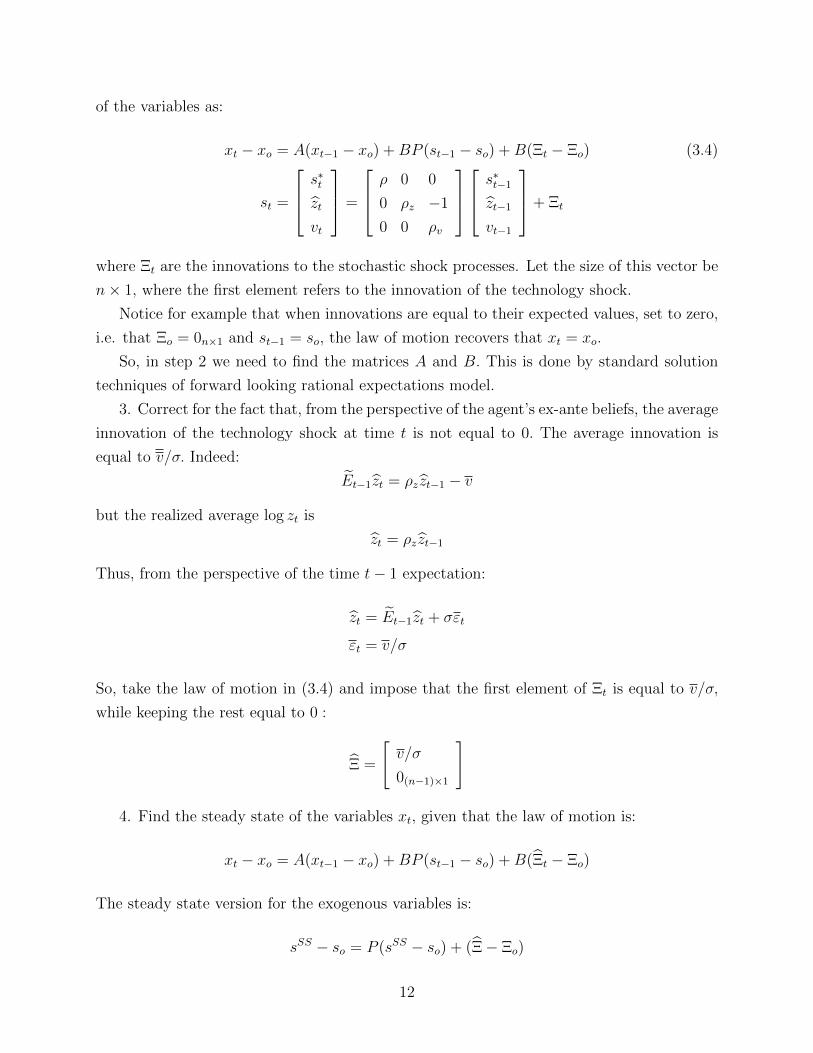
4.1.2 Households
The model described here is a special case of the general formulation of recursive multiple
priors of section 2. In particular, recall the recursive representation in (2.1), where preferences
were defined over uncertain streams of consumption C = (Ct)∞t=0, where Ct : St → <n and n
is the number of goods. In the model described here, there are 2 goods, the consumption of
the final good Yt and leisure. We then only have to define the per-period felicity function,
which for agent i is:
ui (Ct) = ζc,t
{log(Ct+s − θCt+s−1)− ζL,t+s
ψL1 + σL
l1+σLi,t+s
}. (4.5)
Here, ζc,t denotes an intertemporal preference shock, ζL,t is an intratemporal labor supply
shock, θ is an internal habit parameter, Ct denotes individual consumption of the final good
and li,t denotes a specialized labor service supplied by the household. Also, ψL > 0 is a
parameter.1 The two preference shocks follow the time series representation:
log(ζc,t) = ρζc log(ζc,t−1) + ζxc,t
log(ζL,t) = ρζL log(ζL,t−1) + ζxL,t,
where ζxc,t is i.i.d.N(0, σ2ζc
) and ζxl,t is is i.i.d.N(0, σ2ζl
).
Utility follows a recursion similar to (2.1):
Ut(c; st
)= ui (ct, ct−1) + β min
p∈P(st)Ep [Ut+1 (c; st, st+1)] , (4.6)
Let the solution to the minimization problem in (4.6) be denoted by p0. This minimizing
p0 is the same object that appears in the expectation operator of equations (4.4) and (4.2).
The type of Knightian uncertainty we consider in this model is over the transitory
technology level. In section 4.1.1, we described the production side of the economy and
showed where technology enters this economy. Ambiguity here is reflected by the set of one-
1Note that consumption is not indexed by i because we assume the existence of state contingent securitieswhich implies that in equilibrium consumption and asset holdings are identical across households.
16

step ahead conditional beliefs P (st) about the future transitory technology. We follow the
description in section 2 to describe the stochastic process. Specifically, we will assume that
there is time-varying ambiguity about the future technology. This time-variation is captured
by an exogenous component vt. The true dynamics of the transitory productivity shock εt
can be represented by an AR(1) process:
log εt = ρε log εt−1 + σεεxt . (4.7)
The set Pt of one step conditional beliefs about future technology can then be represented
by the family of processes:
log εt+1 = ρε log εt + σεεxt+1 + at (4.8)
at ∈ [−vt,−vt + 2|vt|] (4.9)
vt+1 = (1− ρv) v + ρvvt + σvvxt+1 (4.10)
where the shocks εz and εv are iid and normally distributed shock with mean zero and
variances σ2ε and σ2
v , respectively. As in Section 2, we assume that the agent knows the
evolution of vt, but that he is not sure whether the conditional mean of log εt+1 is really
ρε log εt. Instead, the agent allows for a range of intercepts. If vt is higher, then the agent is
less confident about the mean.of log εt+1 – his belief set is larger.
In this model, it is easy to what is the worst-case scenario, i.e. what is the belief about at
that solves the minimization problem in (4.6). In section 3 we described a general procedure
to find the worst-case belief. In the present model, the environment (given by B, x′ u and
G in the general formulation of section 2) is such that, under expected utility and rational
expectations, a first order solution provides a satisfactory approximation to the equilibrium
dynamics. In this environment, it is easy to check that the value function, under expected
utility, is increasing in the innovation εxt . This monotonicity implies that the worst-case
scenario belief that solves the mininimization problem in (4.6) is given by the lower bound
of the set [−vt,−vt + 2|vt|]. Intuitively, it is natural that the agents take into account that
the worst case is always that the mean of productivity innovations is as low as possible.
The laws of motion in (4.8) and (4.10) are linear. To maintain the interpretation that at
is the worst-case scenario solution to the minimization problem, vt should be positive. Thus,
it is useful not to have vt become negative very often. We are then guided to parameterize
the ambiguity process in the following way. We compute the unconditional variance of the
process in (4.10) and insist that the mean level of ambiguity is high enough so that even a
large negative shock to vt of m unconditional standard deviations away from the mean will
17

remain in the positive domain. We can write this constraint as:
v ≥ mσv√
1− ρ2v
(4.11)
The formula in (4.11) provides a constraint on our parameterization. If the constraint is
binding, then, for a given m, there is a fixed relationship on our parameterization between
v, σv and ρv. In that case, we are left with essentially choosing two out of three parameters.
The household accumulates capital subject to the following technology:
Kt+1 = (1− δ)Kt +
[1− S
(ζI,t
ItIt−1
)]It,
where ζI,t is a disturbance to the marginal efficiency of investment with mean unity, Kt is the
beginning of period t physical stock of capital, and It is period t investment. The function S
reflects adjustment costs in investment. The function S is convex, with steady state values
of S = S ′ = 0, S ′′ > 0. The specific functional form for S(.) that we use is:
S
(ζI,t
ItIt−1
)= exp
[√S ′′
2
(ζI,t
ItIt−1
− 1
)]+ exp
[−√S ′′
2
(ζI,t
ItIt−1
− 1
)]− 2
The marginal efficiency of investment follows the process:
log(ζi,t) = ρζI log(ζi,t−1) + ζxi,t,
where ζxi,t is i.i.d.N(0, σ2ζI
).
Households own the physical stock of capital and rent out capital services, Kt, to a
competitive capital market at the rate Ptrkt , by selecting the capital utilization rate ut:
Kt = utKt,
Increased utilization requires increased maintenance costs in terms of investment goods per
unit of physical capital measured by the function a (ut) . The function a(.) is increasing and
convex, a (1) = 0 and ut is unity in the nonstochastic steady state. We assume that a′′ (u) =
σark, where rk is the steady state value of the rental rate of capital. Then, a′′ (u) /a′ (u) = σa
is a parameter that controls the degree of convexity of utilization costs.
The ith household’s budget constraint is:
PtCt + PtIt
µΥ,tΥt+Bt = Bt−1Rt−1 + PtKt[r
kt ut − a(ut)Υ
−t] +Wt,ilt,i − TtPt
18

where Bt are holdings of government bonds, Rt is the gross nominal interest rate and Tt
is net lump-sum taxes.
When we specify the budget constraint, we will assume that the cost, in consumption
units, of one unit of investment goods, is (ΥtµΥ,t)−1. Since the currency price of consumption
goods is Pt, the currency price of a unit of investment goods is therefore, Pt (ΥtµΥ,t)−1. The
stationary component of the relative price of investment follows the process:
log(µΥ,t/µΥ) = ρµΥlog(µΥ,t−1/µΥ) + µxΥ,t,
where µxΥ,t is i.i.d.N(0, σ2µΥ
).
4.1.3 The government
The market clearing condition for this economy is:
Ct +It
µΥ,tΥt+Gt = Y G
t
where Gt denotes government expenditures and Y Gt is our definition of measured GDP,
i.e. Y Gt ≡ Yt − a(ut)Υ
−tKt. We model government expenditures as Gt = gtz∗t , where gt is
a stationary stochastic process. This way of modeling Gt helps to ensure that the model
has a balanced growth path. The fiscal policy is Ricardian. The government finances Gt by
issuing short term bonds Bt and adjusting lump sum taxes Tt.The law of motion for gt is:
log(gt/g) = ρg log(gt−1/g) + gxt
where gxt is.i.d.N(0, σ2g).
The nominal interest rate Rt is set by a monetary policy authority according to the
following feedback rule:
Rt
R=
(Rt−1
R
)ρR [(πtπ
)aπ (Y Gt
Y ∗t
)ay ( Y Gt
µ∗zYGt−1
)agy]1−ρR
exp(εR.t),
where εR.t is a monetary policy shock i.i.d.N(0, σ2εR
).
4.1.4 Model Solution
The model economy fluctuates along a stochastic growth path. Some variables are station-
ary: the nominal interest rates, the long-term interest rate, inflation and hours worked.
Consumption, real wages and output grow at the rate determined by z∗t . The capital stock
19
and investment grow faster, due to increasing efficiency in the investment producing sector,
at a rate determined by z∗t Υt, with Υ > 1. The solution of our model with ambiguity follows
the general steps described in section 3.The solution of our model builds on the standard
approach to solve for a rational expectations equilibrium with the difference that we need
to take into account that the worst-case scenario expectations do not materialize on average
ex-post. Therefore, the solution involves the following procedure. First, we solve the model
as a rational expectations model in which expectations are correct on average. Here we
follow the standard approach of solving these type models: we rewrite the model in terms of
stationary variables by detrending each variable using its specific trend growth rate. Then
we find the non-stochastic steady state for this detrended system and construct a log-linear
approximation around it. We then solve the resulting linear system of rational expectations
equations. With that law of motion in hand, we then correct for the fact that the true
dynamics of the productivity process follow the process in (4.7) in which at = 0.
The model has 9 fundamental shocks:
[εxt , µ
x,∗z,t , εR.t, g
xt , µ
xΥ,t, λ
xf,t, ζ
xI,t, ζ
xl,t, ζ
xc,t
]and the ambiguity shock vxt .
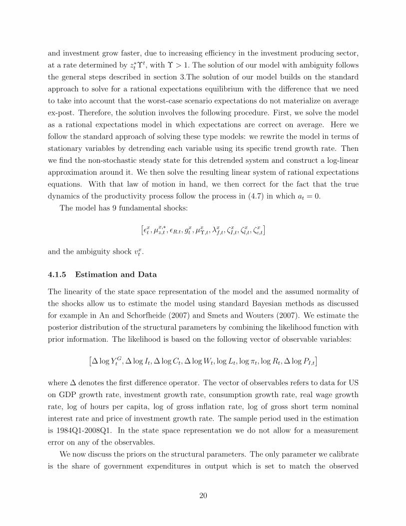
4.1.5 Estimation and Data
The linearity of the state space representation of the model and the assumed normality of
the shocks allow us to estimate the model using standard Bayesian methods as discussed
for example in An and Schorfheide (2007) and Smets and Wouters (2007). We estimate the
posterior distribution of the structural parameters by combining the likelihood function with
prior information. The likelihood is based on the following vector of observable variables:
[∆ log Y G
t ,∆ log It,∆ logCt,∆ logWt, logLt, log πt, logRt,∆ logPI,t]
where ∆ denotes the first difference operator. The vector of observables refers to data for US
on GDP growth rate, investment growth rate, consumption growth rate, real wage growth
rate, log of hours per capita, log of gross inflation rate, log of gross short term nominal
interest rate and price of investment growth rate. The sample period used in the estimation
is 1984Q1-2008Q1. In the state space representation we do not allow for a measurement
error on any of the observables.
We now discuss the priors on the structural parameters. The only parameter we calibrate
is the share of government expenditures in output which is set to match the observed
20

empirical ratio of 0.22. The rest of the structural parameters are estimated. The priors on
the parameters not related to ambiguity and thus already present in the standard medium
scale DSGE are broadly in line with those adopted in previous studies (e.g. Justiniano et al.
(2010), Christiano et al. (2010b)). The prior for each of the autocorrelation parameter of
the shock processes is a Beta distribution with a mean of 0.5 and a standard deviation of
0.15.2 The prior distribution for the standard deviation of the 9 fundamental shocks is an
Inverse Gamma with a mean of 0.01 and a standard deviation of 0.01.
Regarding the choice over the ambiguity parameters, recall the discussion in 4.1.2. In
preliminary estimations of the model, we find that the constraint in (4.11) between the
amount of unconditional volatility and mean ambiguity is binding.3 With equality, the
constraint implies that we can estimate two parameters out of the three: v, σv and ρv. We
choose to work with the following scaling between the mean amount of ambiguity and the
standard deviation of the technology shock
v =σεn
(4.12)
Given this scaling, the binding constraint in (4.11) implies that:
σv =σεn
√1− ρ2
v
m
We fix m = 2 so that a negative shock of two unconditional standard deviations is still in
the positive domain. So, the structural parameters to be estimated are n and ρv.
Alternatively, instead of the scaling in (4.12), we could estimate directly the parameters
ρv and σv. The mean ambiguity would then be given by the binding constraint in (4.11). We
find that the results are very insensitive to this choice. An advantage of the scaling in (4.12)
is that it shows a direct link between how much ambiguity about the mean innovation σεεxt
and the standard deviation of that innovation.
In the benchmark model, the prior on the scaling parameter n is a Gamma distribution
with mean 4 and standard deviation equal to 2. The prior is loose and it allows a wide range
of plausible values. The mean is based on a statistical consideration related to the concept
of detection error probability (see Hansen and Sargent (2008)). A value of 4 corresponds to
2The only exception is the prior on the autocorrelation of the price markup shock, for which the standarddeviation is set to 0.05.
3More precisely, if the three parameters characterizing ambiguity are separately estimated we find that theimplied unconditional volatility of the vt process is so large that it implies very frequent negative realizationsto vt. Additionally there are further issues of identification: if we do not fix other structural parameters, suchas β, we can easily run into identification problems of v. This is a further reason to impose a relationshipbetween the ambiguity parameters.
21

a detection probability of 10% when the sample size is equal to 200. The prior on ρv follows
the pattern of the other autocorrelation coefficients and is a Beta distribution with a mean
of 0.5 and a standard deviation of 0.15.
The prior and posterior distributions are described in Table 2. The posterior estimates
of our structural parameters that are unrelated to ambiguity are in line with previous
estimations of such medium scale DSGE models (Del Negro et al. (2007), Smets and Wouters
(2007), Justiniano et al. (2010), Christiano et al. (2010b)). These parameters imply that
there are significant ‘frictions’ in our model: price and wage stickiness, investment adjustment
costs and internal habit formation are all substantial. The estimated policy rule is inertial
and responds strongly to inflation but also to output gap and output growth. Given that
these parameters have been extensively analyzed in the literature, we now turn attention to
the role of ambiguity in our estimated model.
4.2 Results
We evaluate the importance of ambiguity in our model along two dimensions: the steady
state effect of ambiguity and its role in business cycle fluctuations. We will argue that
ambiguity plays an important part along both of these dimensions.
4.2.1 Steady state
The posterior mode of the structural parameters of ambiguity implies that the mean level of
ambiguity is
v =σεn
=0.0029
0.19= 0.015
which means that the ambiguity averse agent is on average concerned about a mean one-step
ahead future technology level that is 1.5% lower than the true technology, normalized to 1.
In the long run, the agent expects the technology level to be ε∗, which solves:
log ε∗ = ρε log ε∗ − v.
For the estimated ρε = 0.736, we get that ε∗ = 0.944. Thus, the ambiguity-averse agent
expects under his worst-case scenario evaluations the long run mean technology to be
approximately 6% lower than the true mean.
Based on these estimates we can directly find that the standard deviation of the
innovations to ambiguity is
σv = 0.0026
which is close to the estimated standard deviation of the technology innovations.
22

Our interpretation of the reason why we find a relatively large v is the following: the
estimation prefers to have a large σv because the ambiguity shock provides a channel in the
model that delivers dynamics that seem to be favored by the data. Indeed, as detailed in the
next section, the ambiguity shocks generate comovement between variables that enter in the
observation equation. This is a feature that is strongly in the data and is not easily captured
by other shocks. Given the large role that the fit of the data places on the ambiguity shock,
the implied estimated σv is relatively large. Because of the constraint on the size of the mean
ambiguity in (4.11), this results also in a large required steady state ambiguity. Thus, given
also the estimated σε, the posterior mode for n is small. The picture that comes out of these
estimates is that ambiguity is large in the steady state, it is volatile and persistent.
The estimated amount of ambiguity has substantial effects on the steady state of
endogenous variables. To describe these effects we perform the following calculations. We
fix all the estimated parameters of the model but change the estimated standard deviation
of the transitory technology shock, σε, from its estimated value of σε = 0.0029 to being
equal to 0. When σε = 0, then the level of ambiguity a is also equal to 0. By reporting the
difference between the steady states with σε = σε > 0 and with σε = 0 we calculate the effect
on steady states of fluctuations in transitory technology that goes through the estimated
amount of ambiguity. In Table 1 we present a net percent difference of some variables of
interest between the two cases,.i.e. for a variable X we report 100[XSS,(σε=σε)/XSS,(σε=0)−1],
where XSS,(σε=σε) and XSS,(σε=0) are the steady states of variable X under σε = σε and
respectively σε = 0.
Table 1: Steady state percent difference from zero fluctuations
Variable Welfare Output Capital Consumption Hours Nom.Rate
-7.6 -3.4 -0.68 -2.9 -5.7 -38
As evident from Table 1, the effect of fluctuations in the transitory technology shock
that goes through ambiguity is very substantial. Output, capital, consumption, hours
are all significantly smaller when σε = σε. The nominal interest rate is smaller by 38%,
which corresponds to the quarterly steady state interest rate being lower by 69 basis points.
Importantly, the welfare cost of fluctuations in this economy is also very large, of about
8% of steady state consumption. These effects are much larger than what it is implied by
the standard analysis featuring only risk. By standard analysis we mean the strategy of
shutting down all the other shocks except the transitory technology and computing a second
order approximation of the model in which there is no ambiguity but σε = σε. For such
23
a calculation, we find that the welfare cost of business cycle fluctuations is around 0.01%
of steady state consumption. The effects on the steady state values of the other variables
reported in Table 1 is negligible. This latter result is consistent with the conclusions of the
literature on the effect of business cycle fluctuations and risk.
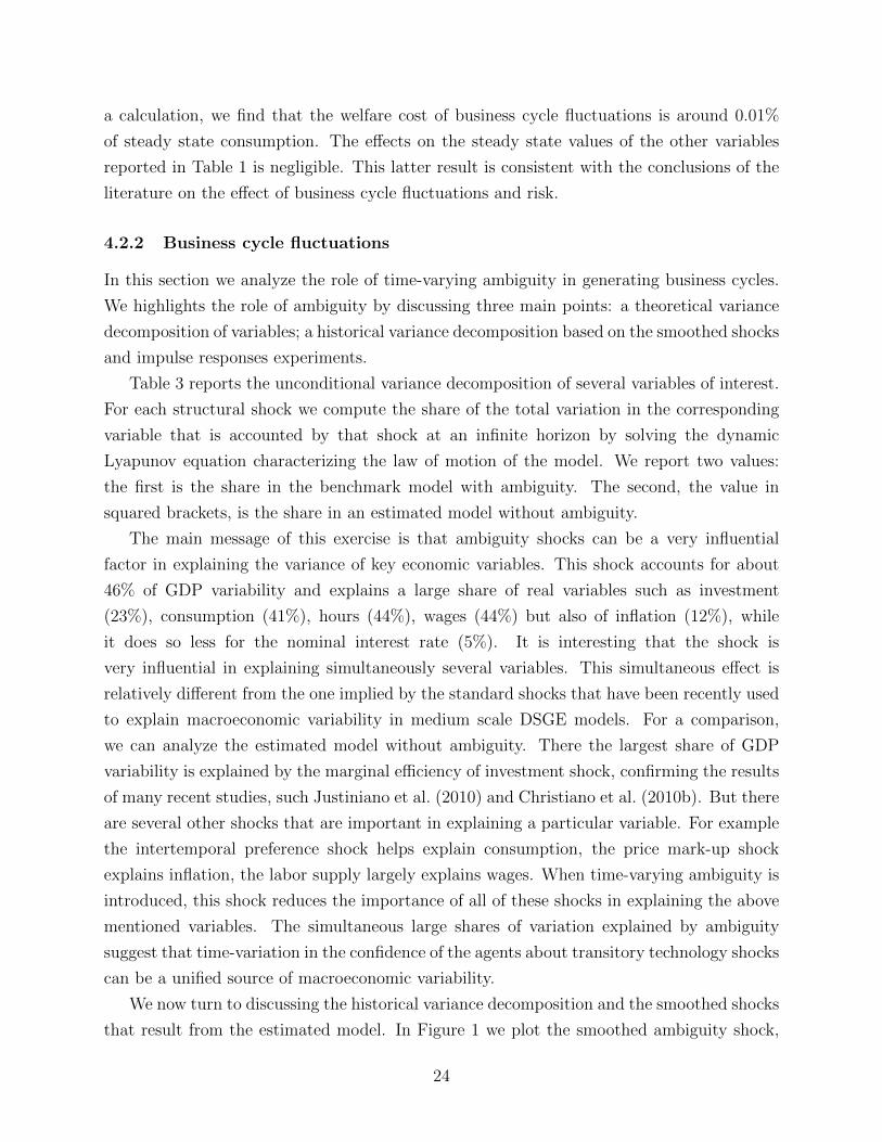
4.2.2 Business cycle fluctuations
In this section we analyze the role of time-varying ambiguity in generating business cycles.
We highlights the role of ambiguity by discussing three main points: a theoretical variance
decomposition of variables; a historical variance decomposition based on the smoothed shocks
and impulse responses experiments.
Table 3 reports the unconditional variance decomposition of several variables of interest.
For each structural shock we compute the share of the total variation in the corresponding
variable that is accounted by that shock at an infinite horizon by solving the dynamic
Lyapunov equation characterizing the law of motion of the model. We report two values:
the first is the share in the benchmark model with ambiguity. The second, the value in
squared brackets, is the share in an estimated model without ambiguity.
The main message of this exercise is that ambiguity shocks can be a very influential
factor in explaining the variance of key economic variables. This shock accounts for about
46% of GDP variability and explains a large share of real variables such as investment
(23%), consumption (41%), hours (44%), wages (44%) but also of inflation (12%), while
it does so less for the nominal interest rate (5%). It is interesting that the shock is
very influential in explaining simultaneously several variables. This simultaneous effect is
relatively different from the one implied by the standard shocks that have been recently used
to explain macroeconomic variability in medium scale DSGE models. For a comparison,
we can analyze the estimated model without ambiguity. There the largest share of GDP
variability is explained by the marginal efficiency of investment shock, confirming the results
of many recent studies, such Justiniano et al. (2010) and Christiano et al. (2010b). But there
are several other shocks that are important in explaining a particular variable. For example
the intertemporal preference shock helps explain consumption, the price mark-up shock
explains inflation, the labor supply largely explains wages. When time-varying ambiguity is
introduced, this shock reduces the importance of all of these shocks in explaining the above
mentioned variables. The simultaneous large shares of variation explained by ambiguity
suggest that time-variation in the confidence of the agents about transitory technology shocks
can be a unified source of macroeconomic variability.
We now turn to discussing the historical variance decomposition and the smoothed shocks
that result from the estimated model. In Figure 1 we plot the smoothed ambiguity shock,
24
as a deviation from its steady state value. The figure first shows that ambiguity is very
persistent. After an initial increase around 1991, which also corresponds to an economic
downturn, the level of ambiguity was low and declining during the 90’s, reaching its lowest
values around 2000. It then increase back to levels close to steady state until 2005. Following
a few years of relatively small upward deviations from its mean, ambiguity spikes starting
in 2008. Ambiguity rapidly increases to reach its peak in 2009Q1, when it is 4 times larger
than its 2008Q1 value. The figure shows a dotted vertical line at 2008Q3, which corresponds
to the Lehman Brothers bankruptcy. Our model interprets the period following 2008Q1
as one in which ambiguity about future productivity has increased dramatically. It thus
offers a formal way to think about time variation in agents confidence in their probability
assessments.
Based on these smoothed path of ambiguity shocks we can now calculate what the model
implies for the historical evolution of endogenous variables. In Figure 2 we compare the
observed data with the hypothetical historical evolution for the growth rate of output,
consumption, investment and inflation when the ambiguity shock is the only shock active
in the model economy. The ambiguity shock implies a path for variables that come close
to matching the data, especially for output and consumption. The model implied path of
investment is less volatile but the correlation with the observed data is still significantly
large. The ambiguity shock also helps explain the historical path for inflation, except for the
last recession where it predicts that inflation should have gone up.
The ambiguity shock generates the three large recessions observed in this sample. Indeed,
if we analyze the smoothed path of the shock in figure 2, the time-varying ambiguity helps
explain the recession of the 1991, the large growth of the 1990’s (as a period of low ambiguity),
and then the recession of 2001. Given that the estimated ambiguity still continues to rise
through 2005, the model misses by predicting a more prolonged recession than in the data,
where output picks up quickly. The rise in ambiguity in 2008 predict in the model that
output, investment and consumption fall. The model matches the fall in consumption, but
fails to generate a large fall in investment.
It is important to highlight that the ambiguity shock implies that in the model consump-
tion and investment comove. Indeed, in the historical decomposition, recessions are times
when both of these variables fall. This is an important effect because standard shocks that
have been recently found to be quantitatively important, such as the marginal efficiency
of investment or intertemporal preference shocks imply a significant negative comovement
between these two components. The negative comovement can be clearly seen in the impulses
responses to shocks to the intertemporal preference and marginal efficiency, reported in
Figures 4 and 5.
25

We conclude this section by analyzing the impulse responses for the ambiguity shock
in the estimated model. As suggested already in the discussion, an increase in ambiguity
generates a recession, in which hours worked, consumption and investment fall. The fact
that this shock predicts comovement between this variables is an important feature that
helps explain why the estimation prefers through the maximization of its likelihood such a
shock. Figure 3 plots the responses to a one standard deviation increase in ambiguity for
the estimated model. On top of the mentioned comovement, the model also predicts a fall
in the price of capital, a fall in the real interest rate and a countercyclical excess return.
We briefly explain these results. The main intuition in understanding the effect of this
shock is to relate it to its interpretation of a news shock. An increase in ambiguity makes the
agent act under a more cautious forecast of the future technology. From an outside observer
that analyzes the agent’s behavior, it seems that this agent acts under some negative news
about future productivity. This negative news interpretation of the increase in ambiguity
helps explain the mechanics and economics of the impulse response. As described in detail
in Christiano et al. (2008), Christiano et al. (2010a), in a rational expectations model, a
negative news about future productivity can produce a significant bust in real economy
while simultaneously generating a fall in the price of capital. This result is reflected in our
impulse response. In our model, the negative news is on average not materialized, because
nothing changed in the true process for technology, as shown in the first panel of Figure
3. However, because of the persistent effect of ambiguity, the economy continues to go
through a prolonged recession. The ex-post excess return, defined as the difference between
the realized return on capital and the risk-free rate, is positive following the period of the
initial increase in ambiguity. The ex-ante excess return is always equal to zero, as we solve a
linearized model. The explanation for the countercyclical excess returns is that the negative
expectation about future productivity does not materialize, so ex-post, capital pays more.
The ex-post excess return is a rational uncertainty premium that ambiguity-averse agents
require to invest in the uncertain asset.
We can conclude that an increase in Knightian uncertainty (ambiguity) generates in our
estimated model a recession, in which consumption, investment and price of capital fall,
while producing countercyclical ex-post excess returns. Given these dynamics, we believe
that time-varying ambiguity can be an important source of observed business cycle dynamics.
26

References
An, S. and F. Schorfheide (2007): “Bayesian analysis of DSGE models,” Econometric
Reviews, 26, 113–172.
Bachmann, R., S. Elstner, and E. Sims (2010): “Uncertainty and Economic Activity:
Evidence from Business Survey Data,” NBER Working Papers 16143, National Bureau of
Economic Research.
Barsky, R. and E. Sims (2011): “News shocks and business cycles,” Journal of Monetary
Economics.
Beaudry, P. and F. Portier (2006): “Stock Prices, News, and Economic Fluctuations,”
American Economic Review, 96, 1293–1307.
Bloom, N., M. Floetotto, and N. Jaimovich (2009): “Really uncertain business
cycles,” Manuscript, Stanford University.
Cagetti, M., L. P. Hansen, T. Sargent, and N. Williams (2002): “Robustness and
Pricing with Uncertain Growth,” Review of Financial Studies, 15, 363–404.
Calvo, G. (1983): “Staggered prices in a utility-maximizing framework,” Journal of
monetary Economics, 12, 383–398.
Christiano, L. (2002): “Solving dynamic equilibrium models by a method of undetermined
coefficients,” Computational Economics, 20, 21–55.
Christiano, L., M. Eichenbaum, and C. Evans (2005): “Nominal Rigidities and the
Dynamic Effects of a Shock to Monetary Policy,” Journal of Political Economy, 113.
Christiano, L., C. Ilut, R. Motto, and M. Rostagno (2008): “Monetary policy and
stock market boom-bust cycles,” ECB Working Papers 955, European Central Bank.
——— (2010a): “Monetary policy and stock market boom-bust cycles,” NBER Working
Papers 16402, NBER.
Christiano, L., R. Motto, and M. Rostagno (2010b): “Financial factors in economics
fluctuations,” ECB Working Papers 1192, European Central Bank.
Del Negro, M., F. Schorfheide, F. Smets, and R. Wouters (2007): “On the fit of
new Keynesian models,” Journal of Business and Economic Statistics, 25, 123–143.
27

Epstein, L. and T. Wang (1994): “Intertemporal asset pricing under Knightian
uncertainty,” Econometrica, 62, 283–322.
Epstein, L. G. and M. Schneider (2003): “Recursive multiple-priors,” Journal of
Economic Theory, 113, 1–31.
——— (2010): “Ambiguity and Asset Markets,” Annual Review of Financial Economics,
forthcoming.
Erceg, C. J., D. W. Henderson, and A. T. Levin (2000): “Optimal monetary policy
with staggered wage and price contracts,” Journal of Monetary Economics, 46, 281–313.
Fernandez-Villaverde, J., P. Guerron-Quintana, J. Rubio-Ramırez, and
M. Uribe (2010): “Risk Matters: The Real Effects of Volatility Shocks,” The American
economic review, forthcoming.
Fernandez-Villaverde, J. and J. Rubio-Ramirez (2007): “Estimating Macroeco-
nomic Models: A Likelihood Approach,” Review of Economic Studies, 74, 1059–1087.
Fernandez-Villaverde, J. and J. Rubio-Ramırez (2010): “Macroeconomics and
volatility: Data, models, and estimation,” NBER Working Papers 16618, National Bureau
of Economic Research.
Gilboa, I. and D. Schmeidler (1989): “Maxmin Expected Utility with Non-unique
Prior,” Journal of Mathematical Economics, 18, 141–153.
Hansen, L., T. Sargent, and T. Tallarini (1999): “Robust permanent income and
pricing,” Review of Economic Studies, 66, 873–907.
Hansen, L. P. and T. J. Sargent (2008): Robustness, Princeton University Press.
Jaimovich, N. and S. Rebelo (2009): “Can News about the Future Drive the Business
Cycle?” The American economic review, 99, 1097–1118.
Justiniano, A. and G. Primiceri (2008): “The Time-Varying Volatility of
Macroeconomic Fluctuations,” The American Economic Review, 98, 604–641.
Justiniano, A., G. Primiceri, and A. Tambalotti (2010): “Investment shocks and
the relative price of investment,” Review of Economic Dynamics.
Schmitt-Grohe, S. and M. Uribe (2008): “What’s News in Business Cycles,” NBER
Working Papers 14215, NBER.
28

Smets, F. and R. Wouters (2007): “Shocks and frictions in US business cycles: A
Bayesian DSGE approach,” The American Economic Review, 97, 586–606.
29
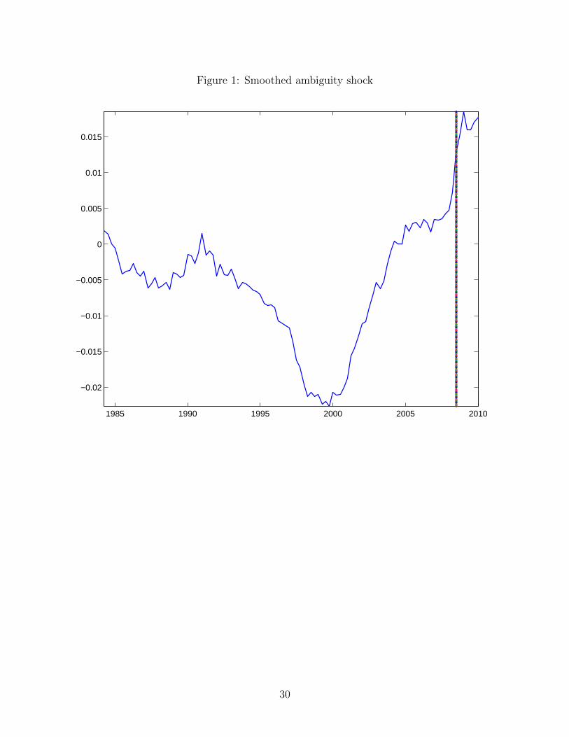
Figure 1: Smoothed ambiguity shock
1985 1990 1995 2000 2005 2010
−0.02
−0.015
−0.01
−0.005
0
0.005
0.01
0.015
30

Figure 2: Historical shock decomposition
1985 1990 1995 2000 2005
−0.06
−0.04
−0.02
0
0.02
Output Growth
Data (year over year)
Model implied: only ambiguity shock
1985 1990 1995 2000 2005
−0.04
−0.03
−0.02
−0.01
0
0.01
0.02
Consumption Growth
1985 1990 1995 2000 2005−0.25
−0.2
−0.15
−0.1
−0.05
0
0.05
Investment Growth
1985 1990 1995 2000 2005
−0.02
−0.01
0
0.01
Inflation
31

Table 2: Priors and Posteriors for structural parameters
Parameter Description Prior Posterior
Type Mean St.dev Mode St.devα Capital share B 0.4 0.02 0.318 0.014δ Depreciation B 0.025 0.001 0.0245 0.001100(β−1 − 1) Discount factor G 0.3 0.05 0.356 0.04100(µ∗z − 1) SS net growth rate N 0.4 0.08 0.45 0.06100(µΥ − 1) SS price of investment net growth rate N 0.4 0.08 0.45 0.01π − 1 SS net inflation N 0.006 0.002 0.01 0.001ξp Calvo prices B 0.375 0.1 0.843 0.02ξw Calvo wages B 0.375 0.1 0.635 0.06S′′
Investment adjustment cost G 10 5 10.26 3.47σa Capacity utilization G 2 1 1.21 0.64aπ Weight on inflation in Taylor rule N 1.7 0.3 2.2 0.19ay Weight on output in Taylor rule N 0.15 0.05 0.1 0.04agy Weight on output growth in Taylor rule N 0.15 0.05 0.23 0.04ρR Coefficient on lagged interest rate B 0.5 0.15 0.84 0.01λf − 1 SS price markup N 0.2 0.05 0.22 0.04λw − 1 SS wage markup N 0.2 0.05 0.156 0.05θ Internal habit B 0.5 0.1 0.78 0.04σL Curvature on disutility of labor G 2 1 2.65 0.9n Level ambiguity scale parameter G 4 2 0.19 0.06ρε Transitory technology B 0.5 0.15 0.736 0.08ρµ∗z Persistent technology B 0.5 0.15 0.439 0.11ρζl Marginal efficiency of investment B 0.5 0.15 0.657 0.06ρζL Labor supply B 0.5 0.15 0.42 0.1ρλf Price mark-up B 0.5 0.05 0.465 0.05ρg Government spending B 0.5 0.15 0.942 0.01ρµΥ
Price of investment B 0.5 0.15 0.955 0.01ρζc Intertemporal Preference B 0.5 0.15 0.727 0.08ρv Level Ambiguity B 0.5 0.15 0.937 0.01σε Transitory technology IG 0.01 0.01 0.0029 0.0004σµ∗z Persistent technology IG 0.01 0.01 0.0062 0.001σζl Marginal efficiency of investment IG 0.01 0.01 0.023 0.002σζL Labor supply IG 0.01 0.01 0.005 0.002σλf Price mark-up IG 0.005 0.01 0.004 0.001σg Government spending IG 0.01 0.01 0.019 0.0015σµΥ
Price of investment IG 0.01 0.01 0.003 0.0002σεR Monetary policy shock IG 0.005 0.01 0.0014 0.0001σζc Intertemporal Preference IG 0.01 0.01 0.02 0.0035
Notes: B refers to the Beta distribution, N to the Normal distribution, G to the Gammadistribution, and IG to the Inverse-gamma distribution.
32

Table 3: Theoretical variance decomposition
Shock\Variable Output Cons. Investm. Hours Inflation Int. rate Wage
TFP Ambiguity (vt) 46.12 41.58 23.58 44 12 4.68 44[-] [-] [-] [-] [-] [-] [-]
Transitory technology (εt) 0.18 0.11 0.13 2.17 1.44 0.75 0.09[0.43] [0.34] [0.21] [2.86] [1.07] [0.65] [0.14]
Persistent technology (µ∗z,t) 7.39 23.14 1 5 8.5 5.7 23.29[6.5] [24.33] [1.3] [6.08] [2.88] [3.12] [25.3]
Government spending (gt) 2.84 6 2.2 5.37 1.5 3.75 0.48[3.8] [7.39] [1.24] [7.15] [0.88] [2.84] [0.38]
Price mark-up (λf,t) 0.4 0.2 0.33 0.5 35.86 9.2 3[3] [1.68] [1.8] [3.28] [62.9] [19.1] [11.3]
Monetary policy (εR.t) 1.28 0.75 1 1.6 3.47 22.8 0.55[2.7] [1.8] [1.47] [3] [1.82] [25.4] [1.4]
Price of investment (µΥ,t) 2 1.68 5 0.28 0.32 0.9 1[2.7] [2.24] [4.66] [0.57] [0.37] [0.7] [1.33]
Preference (ζc,t) 2.14 12.8 1.83 3.26 3.64 6.1 0.66[4.3] [34.5] [2.53] [6.1] [4.5] [8.37] [2.12]
Efficiency of investment (ζI,t) 31.56 9.8 60.66 30.34 13.72 32.9 7.93[66.8] [19.8] [82.15] [60.13] [8.3] [28] [16.6]
Labor supply (ζL,t) 6 3.87 4.25 7.57 19.54 13.2 18.8[9.7] [7.9] [4.6] [10.8] [17.2] [11.8] [41.29]
Note: For each variable, the first row of numbers refers to the variance decomposition in theestimated model with ambiguity. The numbers in the second row, in squared brackets, referto the estimated model without ambiguity.
33

Figure 3: Impulse response: ambiguity
10 20 30 40−1
−0.5
0
0.5
1technology
perc
ent d
evia
tion
from
ss
10 20 30 40
5
10
15
ambiguity
10 20 30 40−0.6
−0.5
−0.4
−0.3
−0.2
GDP
10 20 30 40
−0.5
−0.4
−0.3
−0.2Consumption
perc
ent d
evia
tion
from
ss
10 20 30 40
−1
−0.8
−0.6
−0.4
−0.2
Investment
10 20 30 40
−0.6
−0.4
−0.2
Hours worked
10 20 30 400
5
10
15
ex−post excess return
perc
ent d
evia
tion
from
ss
10 20 30 40−0.2
−0.1
0
0.1
price of capital
10 20 30 401.1
1.15
1.2
1.25
1.3
Net real interest rate
Ann
ualiz
ed, p
erce
nt
34

Figure 4: Impulse response: efficiency of investment
10 20 30 40
0.5
1
1.5
2
Marginal efficiency of investment
perc
ent d
evia
tion
from
ss
10 20 30 40−1
−0.5
0
0.5
1ambiguity
10 20 30 40
−0.6
−0.4
−0.2
GDP
10 20 30 40
−0.2
−0.1
0
0.1
Consumption
perc
ent d
evia
tion
from
ss
10 20 30 40
−2
−1
0Investment
10 20 30 40
−0.6
−0.4
−0.2
0
Hours worked
10 20 30 40−1
−0.5
0
0.5
1ex−post excess return
perc
ent d
evia
tion
from
ss
10 20 30 40
0.1
0.2
0.3
0.4
0.5
price of capital
10 20 30 40
1.2
1.3
1.4Net real interest rate
Ann
ualiz
ed, p
erce
nt
35

Figure 5: Impulse response: intertemporal preference
10 20 30 40
0.5
1
1.5
2
Intertemporal preference shock
perc
ent d
evia
tion
from
ss
10 20 30 40−1
−0.5
0
0.5
1ambiguity
10 20 30 40
0
0.1
0.2
GDP
10 20 30 40
0
0.2
0.4
0.6Consumption
perc
ent d
evia
tion
from
ss
10 20 30 40
−0.3
−0.2
−0.1
Investment
10 20 30 40
0
0.1
0.2
Hours worked
10 20 30 40−1
−0.5
0
0.5
1ex−post excess return
perc
ent d
evia
tion
from
ss
10 20 30 40
−0.1
−0.05
0
price of capital
10 20 30 401.3
1.35
1.4
Net real interest rate
Ann
ualiz
ed, p
erce
nt
36