Ambiguous Business Cycles∗

Cosmin IlutDuke University

Martin SchneiderStanford University

November 2011

Abstract

This paper considers business cycle models with agents who are averse not only torisk, but also to ambiguity (Knightian uncertainty). Ambiguity aversion is describedby recursive multiple priors preferences that capture agents’ lack of confidence inprobability assessments. While modeling changes in risk typically calls for higher orderapproximations, changes in ambiguity in our models work like changes in conditionalmeans. Our models thus allow for uncertainty shocks but can still be solved andestimated using simple 1st order approximations. In an otherwise standard businesscycle model, an increase in ambiguity (that is, a loss of confidence in probabilityassessments), acts like an ‘unrealized’ news shock: it generates a large recessionaccompanied by ex-post positive excess returns.

1 Introduction

How do changes in aggregate uncertainty affect the business cycle? The standard framework

of quantitative macroeconomics is based on expected utility preferences and rational expec-

tations. A change in uncertainty is then typically modeled as an anticipated change in risk,

followed by a change in the magnitude of realized shocks. Indeed, expected utility agents think

about the uncertain future in terms of probabilities. An increase in uncertainty is described

by the anticipated increase in a measure of risk (for example, the conditional variance of a

shock or the conditional probability of a disaster). Moreover, rational expectations implies

that agents’ beliefs coincide with those of the econometrician (or model builder). As a result,

an anticipated increase in risk is followed on average by unusually large shocks, reflecting

the higher variance of shocks or the larger likelihood of disasters.

∗We would like to thank George-Marios Angeletos, Francesco Bianchi, Nir Jaimovich, AlejandroJustiniano, Christian Matthes, Fabrizio Perri, Giorgio Primiceri, Bryan Routledge, Juan Rubio-Ramirez andRafael Wouters, as well as workshop and conference participants at Boston Fed, Carnegie Mellon, CREI,Duke, ESSIM (Gerzensee), Federal Reserve Board, NBER Summer Institute, Ohio State, Rochester, SanFrancisco Fed, SED (Ghent), Stanford, UC Santa Barbara and Yonnsei for helpful discussions and comments.

1

This paper studies business cycle models with agents who are averse to ambiguity

(Knightian uncertainty). Ambiguity averse agents do not think in terms of probabilities

– they lack the confidence to assign probabilities to all relevant events. An increase in

uncertainty may then correspond to a loss of confidence that makes it more difficult to

assign probabilities. Formally, we describe preferences using multiple priors utility (Gilboa

and Schmeidler (1989)). Agents act as if they evaluate plans using a worst case probability

drawn from a set of multiple beliefs. A loss of confidence is captured by an increase in

that set of beliefs. It could be triggered, for example, by worrisome information about the

future. Conversely, an increase in confidence is captured by shrinkage of the set of beliefs –

agents might learn reassuring information that moves them closer toward thinking in terms

of probabilities. In either case, agents respond to a change in confidence if the worst case

probability used to evaluate actions also changes.

The paper proposes a simple and tractable way to incorporate ambiguity and shocks

to confidence into a business cycle model. At every date, agents’ set of beliefs about an

exogenous shock, such as an innovation to productivity, is parametrized by an interval of

means centered around zero. A loss of confidence is captured by an increase in the width of

the interval; in particular, the “worst case” mean becomes worse. Conversely, an increase in

confidence is captured by a narrowing of the interval and thereby a better worst case mean.

Since agents take actions based on the worst case mean, a change in confidence works like

news shock: an agent who gains (loses) confidence responds as if he had received good (bad)

news about the future.

The difference between a change in confidence and news is that the latter is followed, at

least on average, by a shock realization that validates the news. For example, bad news is

on average followed by bad outcomes. A loss of confidence, however, need not be followed

by a bad outcome. Information that triggers a loss of confidence affects agents’ perception

of future shocks, described by their (subjective) set of beliefs. It does not directly affect

properties of the distribution of realized shocks (such as the direction or magnitude of the

shocks). A connection between confidence and realized shocks occurs only if the two are

explicitly assumed to be correlated.

We study ambiguity and confidence shocks in economies that are essentially linear. The

key property is that the worst case means supporting agents’ equilibrium choices can be

written as a linear function of the state variables. It implies that equilibria can be accurately

characterized using first order approximations. In particular, we can study agents’ responses

to changes in uncertainty, as well as time variation in uncertainty premia on assets, without

resorting to higher order approximations. This is in sharp contrast to the case of changes in

risk, where higher order solutions are critical. We illustrate the tractability of our method

2

by estimating a medium scale DSGE model with ambiguity about productivity shocks.

The effects of changes in confidence are what one would expect from changes in uncer-

tainty. For example, a loss of confidence about productivity generates a wealth effect – due to

more uncertain wage and capital income in the future, and also a substitution effect since the

return on capital has become more uncertain. The net effect on macroeconomic aggregates

depends on the details of the economy. In our estimated medium scale DSGE model, a

loss of confidence generates a recession in which consumption, investment and hours decline

together. In addition, a loss of confidence generates increased demand for safe assets, and

opens up a spread between the returns on ambiguous assets (such as capital) and safe assets.

Business cycles driven by changes in confidence thus give rise to countercyclical spreads or

premia on uncertain assets.

To quantify the effects of ambiguity shocks in driving the US business cycle, we incor-

porate ambiguity averse households into an otherwise standard medium scale DSGE model

based on Christiano et al. (2005) and Smets and Wouters (2007). Agents view neutral

productivity shocks as ambiguous and their confidence about productivity varies over time,

a type of “uncertainty shock”. Even in the presence of such uncertainty shocks, standard

linearization methods can be used to solve the model and ease its Bayesian estimation. The

main results are that the estimated confidence process (i) is persistent and volatile, (ii) has

large effects on the steady state of endogenous variables, with welfare costs of ambiguity

about 15% of steady state consumption, (iii) accounts for a sizable fraction of the variance

in output - about 30% at business cycle frequencies and about 55% overall, (iv) generates

positive comovement between consumption, investment. It is this positive comovement that

distinguishes confidence shocks from other shocks and leads the estimation to assign an

important role to confidence in driving the business cycle.

We emphasize that changes in confidence can also generate booms that look “exuberant”,

in the sense that output and employment are unusually high and asset premia are unusually

low, while fundamentals such as productivity are close to their long run average. An

exuberant boom occurs in our model whenever there is a persistent shift in confidence above

its mean. While agents in the model behave on average as if they are pessimistic, what

matters for the nature of booms and busts is how variables move relative to model-implied

averages. Confidence jointly moves asset premia and economic activity, thus generating

booms and slumps. Moreover, the fact that agents behave as if they are pessimistic on

average helps explain the magnitude of average asset premia, which are puzzlingly low in

rational expectations models.

While we do not assume rational expectations, we do impose discipline on belief sets by

connecting them to the data generating process we estimate. To describe agents’ perception

3

of a shock, we decompose our own estimated shock distribution into an ambiguous and a

risky component. For the risky component, agents know the probabilities. For the ambiguous

component, they know only the long run empirical moments. When forecasting in the

short run, however, agents realize that the data are consistent with many distinct models.

Discipline comes from requiring that admissible beliefs make “good enough” forecasts on

average, under any data generating process that is consistent with the long run moments.

More models are “good enough” in this sense if the ambiguous component of the data is

more variable. As a result, movements in confidence about a shock are effectively bounded

by the variability of the shock.

Our paper is related to several strands of literature. The decision theoretic literature on

ambiguity aversion is motivated by the Ellsberg Paradox. Ellsberg’s experiments suggest

that decision makers’ actions depend on their confidence in probability assessments – they

treat lotteries with known odds differently from bets with unknown odds. The multiple

priors model describe such behavior as a rational response to a lack of information about

the odds. To model intertemporal decision making by agents in a business cycle model, we

use a recursive version of the multiple priors model that was proposed by Epstein and Wang

(1994) and has recently been applied in finance (see Epstein and Schneider (2010) for a

discussion and a comparison to other models of ambiguity aversion). Axiomatic foundations

for recursive multiple priors were provided by Epstein and Schneider (2003)

Hansen et al. (1999) and Cagetti et al. (2002) study business cycles models with robust

control preferences. The “multiplier” preferences used by these authors assume a smooth

penalty function for deviations of beliefs from some reference belief. This functional form

rules out first order effects of uncertainty. Models of changes in uncertainty with robust

control (for example, Bidder and Smith (2011)) thus rely on higher order approximations, as

do models of changes in risk. In contrast, multiple priors utility is not smooth when belief

sets differ in means. Instead, there can be first order effects of uncertainty – this is exactly

what our approach exploits to generate linear dynamics in response to uncertainty shocks.

Some of the mechanics of our model are reminiscent of rational expectations models with

signals about future “fundamentals” (for example Beaudry and Portier (2006), Christiano

et al. (2008), Schmitt-Grohe and Uribe (2008), Jaimovich and Rebelo (2009), Blanchard et al.

(2009), Christiano et al. (2010a) and Barsky and Sims (2011)). On impact, the response to

a loss of confidence about productivity in our model resembles the response to noise that is

mistaken for bad news about productivity in a model with noisy signals. The difference is

that noise in a signal only matters for agents’ decisions if the typical signal contains enough

news. Put differently, noise matters for the business cycle only if news shocks are also present

and sufficiently important. In contrast, confidence shocks and their role in the business cycle

4

need not be connected to news shocks.1

Confidence shocks can affect agents’ actions (and hence the business cycle) even if they

are uncorrelated with shocks to “fundamentals” (such as productivity) at all leads and lags.

They share this feature with noise shocks as well as with sunspots (for example Farmer

(2009)), stochastic bubbles (Martin and Ventura (2011)) and shocks to higher order beliefs

(Angeletos and La’O (2011)). At the same time, confidence shocks differ from those other

shocks in that they alter agents’ perceived uncertainty of fundamentals. This is typically

reflected in asset premia. Depending on the application, this need not be true for the other

types of shocks.

Recent work on changes in uncertainty in business cycle models has focused on changes

in realized risk – looking either at stochastic volatility of aggregate shocks (see for ex-

ample Fernandez-Villaverde and Rubio-Ramirez (2007), Justiniano and Primiceri (2008),

Fernandez-Villaverde et al. (2010), Basu and Bundick (2011) and the review in Fernandez-

Villaverde and Rubio-Ramırez (2010)), time-varying probability of aggregate disaster (Gou-

rio (2011)) or at changes in idiosyncratic volatility in models with heterogeneous firms (Bloom

et al. (2009), Arellano et al. (2010), Bachmann et al. (2010) and Christiano et al. (2010b)).

We view our work as complementary to these approaches. In particular, confidence shocks

can generate responses to uncertainty – triggered by news, for example – that is not connected

to later realized changes in risk.

The paper proceeds as follows. Section 2 reviews multiple priors utility and shows how

ambiguity about the mean of a bet entails first order effects of uncertainty. Section 3 analyzes

a stylized business cycle model with ambiguity about productivity. Section 4 presents a

general framework for adapting business cycle models to incorporate ambiguity aversion.

Here we show how uncertainty can be studied using linear techniques. Section 5 describes

the estimation of a medium scale DSGE model for the US.

2 Recursive multiple priors

Ellsberg (1961) showed that there is a behaviorally meaningful distinction between risk

(uncertainty with known odds or objectively given probabilities) and ambiguity (unknown

odds). For example, many people strictly prefer to bet on an urn that is known to contain

an equal number of black and white balls than on an urn of unknown composition. Gilboa

and Schmeidler (1989) showed that Ellsberg-type behavior can be derived from a model of

rational choice with axiomatic foundations. Their axioms allow for a “preference for knowing

1This distinction between noise, news and confidence and its observable implications are discussed furtherin Section 3 below.

5

the odds” that is ruled out under expected utility.

For our business cycle application, we use a recursive version of the multiple priors model.

Uncertainty is represented by a period state space S. One element s ∈ S is realized every

period, and the history of states up to date t is denoted by st = (s0, ..., st). Preferences order

uncertain streams of consumption C = (Ct)∞t=0, where Ct : St → <n and n is the number of

goods. Utility for a consumption process C = {Ct} is defined recursively by

Ut(C; st

)= u (Ct) + β min

p∈Pt(st)Ep[Ut+1

(C; st, st+1

)], (2.1)

where Pt (st) is a set of probabilities on S.

Utility after history st is given by felicity from current consumption plus expected

continuation utility evaluated under a “worst case” belief. The worst case belief is drawn

from a set Pt (st) that may depend on the history st. The primitives of the model are the

felicity u, the discount factor β and the entire process of one-step-ahead belief sets Pt (st).

Expected utility obtains as a special case if all sets Pt (st) contain only one belief. More

generally, a nondegenerate set of beliefs captures the agent’s lack of confidence in probability

assessments; a larger set Pt (st) says that the agent is less confident after having observed

history st.

Discussion

The maxmin representation (2.1) is implied by a preference for knowing the odds. Gilboa

and Schmeidler assume that one can observe choice among state contingent consumption

lotteries, as in Anscombe and Aumann (1963) axiomatization of the (subjective) expected

utility model. Lotteries are a source of “objective” uncertainty (known odds) whereas for

the state s there are no objectively given probabilities. Observing choice between state

contingent lotteries can then identify whether or not agents deal with uncertainty about s

as if they think in terms of probabilities.

In particular, the necessary conditions for an expected utility representation in Anscombe

and Aumann (1963) include the independence axiom. It says that C is strictly preferred to

C if and only if any lottery between C and some other plan D is also strictly preferred to a

lottery with the same probabilities on C and D. It implies that an agent who is indifferent

between two consumption plans C and C never strictly prefers a lottery between those two

plans. This latter implication contradicts Ellsberg-type behavior. For example, if one plan

is a hedge for the other then forming a lottery assigns known probabilities to otherwise

6

ambiguous contingencies.2 Put differently, randomizing between two indifferent ambiguous

plans that hedge each other can transform ambiguity into risk, resulting in a strictly more

desirable plan.

Gilboa and Schmeidler show that a maxmin representation of utility follows if indepen-

dence is replaced by two alternative axioms. Uncertainty aversion says that a lottery between

indifferent plans is weakly preferred to either plan. The axiom thus allows (but does not

require) strict preference for the lottery, weakening independence. Certainty independence

says that the independence axiom holds as long as D is constant. This axiom says that strict

preference for a lottery between indifferent plans can occur only if in fact one plan hedges

the other. Randomizing with constant plans is not helpful because constant plans cannot

be hedges. For example, a lottery between an ambiguous plan and its certainty equivalent

is never strictly preferred to the certainty equivalent (and hence the plan itself). The latter

property is shared by the multiple priors and expected utility models.

Epstein and Schneider (2003) provide foundations for the intertemporal model (2.1).

They consider a family of conditional preference orderings, one for each history st. Each

conditional preference ordering satisfies the Gilboa-Schmeidler axioms, suitably modified for

multiperiod plans. Moreover, conditional preferences at different histories are connected

by dynamic consistency.3 The setup of the model also implies consequentialism, that is,

utility from a consumption plan at history st depends only on the consumption promised

in future histories that can still occur after st has been realized. Both dynamic consistency

and consequentialism are intuitive properties that are also satisfied by the standard expected

utility model.

First order effects of uncertainty

Consider the effect of a small increase in uncertainty at a point of certainty. Fix a

constant consumption bundle C, a date t and a nonconstant function f that maps states

into consumption bundles – a “bet” on the state one period ahead at t + 1. Construct an

uncertain consumption plan C by setting Cτ = C for all τ 6= t+ 1, but Ct+1 = C +αf(st+1)

2For example, suppose C pays one if state s occurs and zero otherwise, and C is a perfect hedge for C,that is, it pays one if s does not occur and zero otherwise. Then a lottery between C and C is purely riskyand may thus be preferable to the ambiguous plans C and C.

3In addition to the recursive representation (2.1), the model also allows for a “sequence” representationwhere minimization at every node is over probabilities over future sequences of state s and where thoseprobabilities are updated measure-by-measure by Bayes’ rule.

7

where α is a scalar. We expand utility around certainty (α = 0). For α > 0, we obtain

U(C; st

)= U

(C; st

)+ β min

p∈Pt(st)Ep[u

(C + αf(st+1)

)]

= U(C; st

)+ β

(αu′

(C)Ep0

[f (st+1)] +1

2α2u′′

(C)Ep0 [

f (st+1)2]+ ...

), (2.2)

where higher order terms are omitted and p0 is the belief that achieves the minimum. A

similar expansion holds for α < 0, but the minimizing belief p0 may be different since

consumption depends differently on the state s.

We now compare the welfare effects of small changes in uncertainty by varying α (the

scale of the bet) near zero. To isolate the effect of uncertainty, we focus on bets f such that

for any small α 6= 0, the agent is strictly worse off than at certainty (α = 0). In the case of a

risk averse agent with expected utility (u is strictly concave and Pt (st) = {p0}) this simply

means that the bet f is actuarially fair, or Ep0[f (st+1)] = 0.4 Consider now the magnitude

of the utility loss from an increase in risk as α moves away from zero. The first order term in

(2.2) vanishes, but the second term is negative because of risk aversion. We have restated

the familiar result that, under expected utility, changes in risk have second order effects on

utility near certainty.

Now consider instead a multiple priors agent. In order for such an agent to be worse off

than at certainty for any small α 6= 0 we must have5

minp∈P(st)

Ep [f (st+1)] ≤ 0 ≤ maxp∈P(st)

Epf (st+1) (2.3)

Now assume that the agent perceives ambiguity about the mean and therefore the means

Epf (st+1) are not all zero so that at least one of the inequalities in (2.3) is strict. In other

words, there is ambiguity about whether the bet is fair. Now the first order term in (2.2) need

not vanish. For example, suppose that the lowest mean is strictly negative and consider small

α > 0. The worst case mean must be the negative lower bound: this generates a nonzero

negative first order term which dominates for small α. Changes in ambiguity due to changes

in the interval of means (2.3) thus have first order effects on welfare near certainty. If zero

is in the interior of the interval, then first order effects dominate the welfare calculations for

any α 6= 0.

4Indeed, if f were not fair and had nonzero mean then for small enough α of the same sign as the mean,the first order effect in (2.2) dominates and we obtain higher utility than at α = 0. Conversely, taking fairbets always lowers utility because u is strictly concave.

5Indeed, suppose the mean were of the same sign for all p. Then choosing a small enough α of the samesign as all the means would again deliver more utility than at certainty. Conversely, if (2.3) holds, thentaking the bet lowers utility since u is strictly concave and zero is always a possible choice of mean.

8

3 A stylized example

To illustrate the role of ambiguity in business cycles, we consider a stylized business cycle

model. Our main criterion for this model is simplicity. We abstract from internal propagation

of shocks through endogenous state variables such as capital or sticky prices or wages. For

uncertainty about productivity to have an effect on labor hours and output, we assume

that labor has to be chosen before productivity is known. This introduces an intertemporal

decision that depends on both risk and ambiguity. In fact, with the special preferences and

technology we choose, the effects of both ambiguity and risk can be read off a loglinear closed

form solution, which facilitates comparison.

A representative agent has felicity over consumption and labor hours

U (C,N) =1

1− γC1−γ − βN

where γ is the coefficient of relative risk aversion (CRRA) or equivalently the inverse of the

intertemporal elasticity of consumption (IES). Agents discount the future with the discount

factor β. Setting the marginal disutility of labor equal to β simplifies some algebra below

by eliminating constant terms.

Output Yt is made from labor Nt according to the linear technology.

Yt = ZtNt−1,

where logZt is random. The fruits of labor effort made at date t − 1 thus only become

available at date t. One interpretation is that goods have to be stored for some time before

they can be consumed. It may be helpful to think of the period length as very short, such

as a week.

For simplicity, we assume that log productivity zt = logZt is serially independent and

normally distributed. The productivity process takes the form

zt+1 = µt −1

2σ2u + ut+1 (3.1)

Here u is an iid sequence of shocks, normally distributed with mean zero and variance σ2u.

The sequence µ is deterministic and unknown to agents – its properties are discussed further

below.

Preferences are given by (2.1) with felicity as above. Agents perceive the unknown

component µt to be ambiguous. We parametrize their one-step-ahead set of beliefs at date t

by a set of means µpt ∈ [−at, at]. Here at captures agents’ lack of confidence in his probability

9

assessment of productivity zt+1. We allow confidence itself to change over time to reflect, for

example, news agents receive. We assume an AR(1) process for at:

at+1 = (1− ρa) a+ ρaat + εat+1 (3.2)

with a > 0 and 0 < ρa < 1. The lack of confidence at thus reverts to a long run mean a.

Periods of low at < a represent unusually high confidence in future productivity, whereas at >

a describes periods of unusual lack of confidence. We further assume that εat is independent

of ut.6

Consider now the Bellman equation of the social planner problem

V (Y, a) = maxN

{U (Y,N) + β min

µp∈[−a,a]Ep[V(ezN, a

)]}where tildes indicate random variables and where the conditional distribution of z under

belief p is given by (3.1) with µt = µp. The transition law of the exogenous state variable a

is given by (3.2).

It is natural to conjecture that the value function is increasing in output. The ”worst

case” belief, p0 say, then has mean µp0 = −a. Combining the first order condition for labor

with the envelope condition, we obtain

β = Ep0

[β(ZN

)−γZ

]with µp0 = −a (3.3)

The constant marginal disutility of labor is equal to the marginal product of labor, weighted

by future marginal utility because labor is chosen one period in advance.

3.1 The effect of uncertainty on hours

With our special preferences and technology, optimal hours are independent of current

productivity (or output). Taking logarithms and using normality of the shocks, we can

write the decision rule for hours as

n = − (1/γ − 1)

(a+

1

2γσ2

u

)(3.4)

6We assume that a is an exogenous persistent process, interpreted as the cumulative effect of news thataffect confidence. Epstein and Schneider (2007) and Epstein and Schneider (2008) present a model of learningunder ambiguity that shows how updating affects confidence and Ilut (2009) considers a model of of updatingabout a perpetually changing hidden state. A key feature of those models is that confidence moves slowlywith signals. We thus view a as a reasonable standin to examine the dynamics of confidence in a businesscycle setting. More generally, it could also be interesting to allow for correlation between innovations toconfidence and other shocks. This is omitted here for simplicity.

10

The equation describes the effect of uncertainty on aggregate hours. Uncertainty works the

same way whether it is ambiguity, as measured by a, or risk, as measured by the product of

the quantity of risk σ2u and risk aversion γ.

As usual, an increase in uncertainty has wealth and substitution effects. Consider first

an increase in risk. On the one hand, higher risk lowers the certainty equivalent of future

production, which, in the absence of ambiguity, is given by N exp(−12γσ2

u). Other things

equal, the resulting wealth effect leads the planner to reduce consumption of leisure and

increase hiring. However, higher risk also lowers the risk adjusted return on labor. Other

things equal, the resulting substitution effect leads the planner to reduce hiring. The net

effect depends on the curvature in felicity from consumption, determined by γ. With a strong

enough substitution effect, an increase in risk lowers hiring.

Consider now an increase in ambiguity. When a increases, the planner acts as if expected

future productivity has declined. Mechanically, an increase in ambiguity thus entails wealth

and substitution effects familiar from the analysis of news shocks. The interpretation of

these effects, however, is the same as in the risk case. On the one hand, higher ambiguity

lowers the certainty equivalent of future production, which, in the absence of risk, is given

by N exp (−at). On the other hand, higher ambiguity lowers the uncertainty-adjusted return

on labor. Again, with a strong enough substitution effect an increase in uncertainty lowers

hiring.

Given separable felicity and the iid dynamics of zt, inspection of the Bellman equation

shows that the value function depends on current output only through the utility of consump-

tion – the other terms depend only on the state variable at, not on current productivity or

past hours. It follows that the value function is increasing in output, verifying our conjecture

above. Below, we argue that the ”guess-and-verify” approach to finding the worst case belief

that we have used here to solve the planner problem is applicable much more widely.

The complete dynamics of the model are then given by the productivity equation (3.1)

as well as

yt = zt + nt−1,

nt = − (1/γ − 1)

(at +

1

2γσ2

u

),

at = (1− ρa) a+ ρaat−1 + εat ,

The economy is driven by productivity and ambiguity shocks. Productivity shocks tem-

porarily change output but have no effect on hours. In contrast, ambiguity shocks have

persistent effects on both hours and output.

11

With a strong enough substitution effect (1/γ > 1), a loss of confidence (an increase in

a) generates a recession. During that recession, productivity is not unusually low. Hours

are nevertheless below steady state: since the marginal product of labor is more uncertain,

the planner finds it optimal not to make people work. Conversely, an unusual increase in

confidence – a drop of at below its long run mean – generates a boom in which employment

and output are unusually high, but productivity is not. In other words, a phase of low as will

look to an observer like a wave of optimism, where output and employment surge despite

average productivity realizations.

3.2 Decentralization

Suppose that agents have access to a set of contingent claims. Write qt (z, a) for the date

t price of a claim that pays one unit of consumption at date t + 1 if (zt+1, at+1) = (z, a) is

realized and denote the spot wage by wt. The agent’s date t budget constraint is

Ct +

∫qt (z, a) θt (z, a) d (z, a) = wtNt + θt−1 (zt, at) ,

where θt (z, a) is the amount of claims purchased at t that pays off one unit of the consumption

good if (z, a) is realized at t+ 1. Since aggregate labor is determined one period in advance,

this set of contingent claims completes the market – claims on (z, a) can be used to form

any portfolio contingent on the aggregate state (Y, a).

Assume that there are time invariant functions for prices q (z, a;Y, a) and w (Y, a) as well

as aggregate labor N (Y, a) that depend only on the aggregate state (Y, a). Assume further

that the agent knows those price functions. The Bellman equation is

W (θ, Y, a) = maxC,N,θ′(.)

{U (C,N) + β min

µp∈[−a,a]Ep[W(θ′ (z, a) , ezN (Y, a) , a

)]}w (Y, a)N + θ = C +

∫q (z, a;Y, a) θ′ (z, a) d (z, a)

Conjecture again that utility depends positively on the state variable Y . The worst case

mean is then once more µp = −a and the maximization problem becomes standard.

In particular, prices are related to the agent’s marginal rates of substitution through Euler

equations. Letting fµ (z, a|a) denote the conditional density of the exogenous variables (z, a)

implied by (3.1) and (3.2) with µt = µ, we have

12

w = βC (θ, Y, a)γ (3.5)

q (z, a;Y, a) = βf−a (z, a|a)

(C(θ′ (z, a) , ezN (Y, a) , a

)C (θ, Y, a)

)−γ(3.6)

The wage is equal to the marginal rate of substitution of consumption for hours. State

prices are equal to the marginal rates of substitutions of current for future consumption.

Importantly, state prices are based on the worst case conditional density f−a. This is how

ambiguity aversion contributes to asset premia and how it shapes firms’ decisions in the face

of uncertainty.

For simplicity, we consider two-period lived firms that hire workers only at date t and

sell output only at date t + 1. To pay the wage bill at date t, they issue contingent claims

which they subsequently pay back out of revenue at date t + 1. The profit maximization

problem is

maxN,θ(.)

∫q (z, a;Y, a) (ezN − θ (z, a))d (z, a)

s.t. wN =

∫q (z, a;Y, a) θ (z, a) d (z, a)

As usual, the financial policy of the firm is indeterminate. Substituting the constraint

into the objective, the first order condition with respect to labor equates the wage to the

marginal product of labor

w =

∫q (z, a;Y, a) ezd (z, a) (3.7)

Since labor is chosen one period in advance, the marginal product of labor involves state

prices, which in turn reflect uncertainty perceived by agents. Substituting for prices from

(3.5)-(3.6), we find that the planner’s first order condition for labor (3.3) must hold in any

equilibrium.

From the first order conditions, wages and state prices can be solved out in closed form.

Let Qf (Y, a) =∫q (z, a;Y, a) d (z, a) denote the price of a riskless bond. We can then write

w (Y, a) = βY γ,

Qf (Y, a) = βY γ exp(a+ γσ2

u

),

q (z, a;Y, a) = Qf (Y, a) f 0 (z, a|a) exp

(−1

2σ2u

(a/σ2

u + γ)2 −

(a/σ2

u + γ)(

z − 1

2σ2u

)),

(3.8)

13

where f 0 is the density of the exogenous variables (z, a) if µt = 0.

With utility linear in hours, labor supply is perfectly elastic at a wage tied to current

output. Since output does not react to uncertainty shocks on impact, neither does the wage.

Uncertainty shocks are transmitted to the labor market because asset prices affect labor

demand. The bond price increases with both ambiguity and risk. Intuitively, either type of

uncertainty encourages precautionary savings and thereby lowers the riskless interest rate

rf (Y, a) = − logQf (Y, a) = − log β − γ log Y − a− γσ2u

The price of a claim on a particular state (z, a) is equal to the riskless bond price multiplied

by an “uncertainty neutral” density. We have written the latter as the density for µt = 0

times an exponential term that collects uncertainty premia.

If agents do not care about either type of uncertainty (a = γ = 0), then uncertainty

premia are zero and the exponential term is one. More generally, the relative price of a

“bad” state (that is, lower productivity z) is higher when confidence is lower (or a is higher).

Intuitively, when confidence is lower, then agents value the insurance provided by claims

on bad states more highly. This change in relative prices also affects firms’ hiring decision.

Indeed, since firms can pay out more in good (high z) states, a loss of confidence that makes

claims on good states less valuable increases firms’ funding cost. Conversely, an increase in

confidence makes claims on good states more valuable; lower funding costs then induce more

hiring.

The functional form of the state price density is that of an affine pricing model with “time-

varying market prices of risk” (that is, time varying coefficients multiplying the shocks). This

type of pricing model is widely used in empirical finance. Here time variation in confidence

drives the coefficient a/σ2u + γ on the shock z and thus permits a structural interpretation

of the functional form. A convenient feature of affine models is that conditional expected

returns on many interesting assets are linear functions of the state variables. Consider, for

example, a claim to consumption next period. Its price and excess return are

Qc (Y, a) = βE−a[(ezN (Y, a)

)1−γY γ]

= Qf (Y, a)N (Y, a) exp(−a− γσ2

u

)re (z, Y, a) = log

(ezN (Y, a)

)− logQc (Y, a)− logQf (Y, a)

= z + a+ γσ2u

Long run average excess returns have an ambiguity and a risk component. Moreover, the

conditional expected excess return depends positively on a. In other words, a loss of

confidence not only generates a recession, but also increases the conditional premium on

14

the consumption claim.

3.3 Comparison to news and noise shocks

We have seen that confidence shocks in our model work like unrealized news shocks with

a bias. In this subsection we compare our model with confidence shocks to a rational

expectations model with news and noise shocks. We show that the two models can be

distinguished by considering either quantity moments or asset price data. To this end, we

study a version of the stylized model above in which agents receive noisy signals about future

productivity.

Suppose that, at date t, agents observe a signal about productivity one period ahead.

The joint dynamics of the signal and productivity itself are

st = zt+1 + σsεs,t

zt+1 = −1

2(1− π)σ2

u + ut+1

where the noise εs,t is uncorrelated with all other shocks and π = σ2u/ (σ2

u + σ2s). Since the

conditional variance of var (zt+1|st) is (1− π)σ2u the constant in the second equation ensures

that E [Zt+1|st] = 1. The parameter π indicates how good the signal is: if π = 1 then the

signal reveals tomorrow’s productivity (a pure news shock) whereas π = 0 says that the

signal is worthless (a pure noise shock).

Optimal hours are now

nt = − (1/γ − 1)

(πst −

1

2γ (1− π)σ2

u

)With a strong enough substitution effect, agents work more if a good signal arrives. Of course,

the signal could either reflect good future productivity (news) or a positive realization of εs

(noise). In the news case, the shock will be followed by realized high productivity, but in the

noise case this need not happen (and in fact will not happen on average). Ambiguity shocks

are thus similar to noise shocks in that can they affect actions, but not realized fundamentals.

Nevertheless, it is straightforward to distinguish the news & noise model from the

ambiguity model above. First, consider a simple regression of log productivity on log hours.

In a large sample, we obtain a slope coefficient

β =cov (zt+1, nt)

var (nt)=

− (1/γ − 1) πσ2u

(1/γ − 1)2 π2(σ2u + σ2

s)= −(1/γ − 1)−1

15

In other words, if news matters for employment (γ 6= 1), then employment must forecast

productivity. In contrast, the ambiguity model above does not predict such a relationship.

The point here is that while ambiguity shocks work mechanically like noise shocks, noise

shocks can matter only if there are also enough news shocks, and the presence of news will

be reflected in the regression coefficient.

A second important difference between a news & noise model and the ambiguity model

above lies in the predictions for asset prices. The price formula (3.8) shows that an

econometrician who observes data from the ambiguity model will recover a pricing kernel

that features “time varying market prices of risk”. Such time variation would be reflected

for example in predictability regressions of excess returns on forecasting variables. Moreover,

prices changes can be dominated by changes in confidence which can be uncorrelated with

changes in expected fundamentals, thus leading to “excess volatility”. In contrast a news

model predicts that risk premia are constant and asset prices move mostly with expected

fundamentals.

3.4 Bounding ambiguity by measured volatility

Consider now the connection between the true dynamics of log productivity z in (3.1) and

the agents’ set of beliefs. In our model, productivity consists of two components, the iid

shock u that agents view as risky, and the deterministic sequence µ that agents view as

ambiguous. In line with agents’ lack of knowledge about µ, we do not impose a particular

sequence as “the truth”. Instead, we restrict only the long run average and variability of µ,

and thereby also of productivity z. We then develop a bound on the process at that ensures

that the belief set is “small enough” relative to the variability in the data observed by agents.

For quantitative modeling, the bound imposes discipline on how much the process at can

vary relative to the volatility in the data measured by the modeler.

Consider first the long run behavior of µ. Let I denote the indicator function and let

Φ (.,m, s2) denote the cdf of a univariate normal distribution with mean m and variance s2.

We assume that the empirical distribution of µ converges to that of an iid normal stochastic

process with mean zero and variance σ2µ. Formally, we require that, for any integers k, τ1, ..., τk

and real numbers µ1, ..., µk,

limT→∞

1

T

T∑t=1

I({µt+τj ≤ µj; j = 1, .., k

})=

k∏j=1

Φ(µj; 0, σ2

µ

).

In particular, we assume that for almost every realization of the shocks u, the empirical

second moment 1T

∑Tt=1 µtut converges to zero.

16

For example, if we were to observe µ and record the frequency of the event {µt ≤ µ} then

that frequency would converge to Φ(µ, 0;σ2

µ

). For a two-dimensional example, consider the

frequency of the event {µt ≤ µ1, µt+τ ≤ µ2} – it is assumed to converge to Φ(µ1, 0;σ2

µ

)Φ(µ2, 0;σ2

µ

).

Similarly, recording frequencies of any joint event that restricts elements of µ spaced in time

as described by the τjs always delivers in the long run the cdf of an iid multivariate normal

distribution. At the same time, almost every draw from an iid normal process with mean

zero and variance σ2µ would deliver a sequence µt that satisfies the condition.

We also require that the ambiguous component in the data is not systematically related to

the risky component. In particular, we assume that for almost every realization of the shocks

u, the empirical second moment 1T

∑Tt=1 µtut converges to zero. This has implications for the

long run empirical distribution of log productivity z. Indeed, given a true sequence µ that

satisfies the above condition, then for almost every realization of the shocks u the empirical

mean 1T

∑t zt converges to zero, the empirical variance 1

T

∑t z

2t converges to σ2

z = σ2µ + σ2

u,

and the empirical autocovariances at all leads and lags converge to zero. In other words, to an

econometrician who sees a large sample, the data look like white noise (that is, uncorrelated

with mean zero and variance σ2z) regardless of the true sequence µ.

If an econometrician fits a covariance stationary statistical model to the productivity

data, he thus recovers an iid process with mean zero and variance σ2z . Ambiguity averse

agents look at the data differently. Even though they know the limiting properties of µ and

hence of z, when they make decisions at date t, they are concerned that they do not know the

current conditional mean µt needed to forecast zt+1. They understand that statistical tools

cannot help them learn µt in real time. They deal with their lack of knowledge at date t by

behaving as if they minimize over a set of forecasting rules (that is, a set of one-step-ahead

conditional probabilities) indexed by the interval [−at, at]. It makes sense to assume that

this interval should be smaller the less variable the data are (lower σ2z) and, in particular,

the less variability in the data is attributed to ambiguity as opposed to risk (lower σ2µ).

We thus develop a bound on the process at, denoted amax, that is increasing in σ2µ. The

basic idea is that even the boundary forecasts indexed by ±amax should be “good enough”

in the long run. To define “good enough”, we calculate the frequency with which one of

the boundary forecasting rules is the best forecasting rule in the interval [−amax, amax]. The

forecasting rule with mean amax is the best rule at date t if its mean amax − 12σ2u is closest

to the true conditional mean µt − 12σ2u, that is, if µt ≥ amax. Similarly, the rule −amax is the

best rule if µt ≤ −amax. We now require that the frequency with which µt falls outside the

interval [−amax, amax], thus making the boundary forecasts the best forecasts, converges in

the long run to a number α ∈ (0, 1). Given our assumption on the long run behavior of µ

17

above, the bound is defined by

Φ(amax; 0, σ2

µ

)= α/2

The number α determines the tightness of the bound. For example, α = 5% implies amax ≈2σµ.

The bound amax restricts the variability in the worst case mean relative to measured

volatility in the data. Suppose the variance of the productivity is measured to be σ2z . Denote

by ρ = σ2µ/σ

2z the share of the variability in the data that agents attribute to ambiguity. Then

with α = 5% we require at ≤ 2√ρσz. The bound is tighter if less of the variability in the data

is due to ambiguity. In the extreme case of ρ = 0, the process at must be identically equal

to zero – agents treat all variability in z as risk. In practice, the bound dictates parameter

restrictions on the law of motion for at. In a discrete time model, we cannot impose exactly

that at ∈ [0, 2√ρσz]. However, small enough volatility of εat in (3.2) ensures that those

conditions are virtually always satisfied – this is the approach we follow in our quantitative

work below.

It is interesting to compare how risk and ambiguity affect the long run behavior of business

cycles variables in our simple model. Consider, for example, the empirical mean and variance

of output in a large sample

y = −1

2σ2u − (1/γ − 1)

(a+

1

2γσ2

u

)σ2y = σ2

z + (1/γ − 1)2 var (at)

Here we have used the law of large numbers for u together with our assumptions on µ, which

imply that the long run moments are the same for every possible sequence µ. The bound

puts discipline on the role of ambiguity in explaining business cycles. For example, suppose

that we assume a > 3√var (at) and a + 3

√var (at) < 2

√ρσz in order to keep a almost

always in the interval [0, 2√ρσz]. Together these conditions imply that var (at) < (ρ/9)σ2

z ,

which in turn bounds the share of σ2y that can be contributed by time-varying ambiguity.

4 General framework

4.1 Environment & equilibrium

We consider economies with many individuals i ∈ I and we assume Markovian dynam-

ics. The econometrician’s model of the exogenous state s ∈ S is a Markov chain with

18

transition probabilities p∗ (st). Agent i’s preferences are of the form (2.1) with primitives

(βi, ui, {P i (st)}). Given preferences, it is helpful to write the rest of the economy in fairly

general notation that many typical problems can be mapped into. Consider a recursive

competitive equilibrium. The vector X collects endogenous state variables that are prede-

termined as of the previous date. Let Ai denote a vector of actions taken by agent i. One

action is the choice of consumption and we write ci (Ai) for agent i′s consumption bundle

when his action is Ai. Finally, let Y denote a vector of other endogenous variables not chosen

directly by any agent – this vector will typically include prices, but perhaps also variables

such as government transfers.

The technology and market structure are summarized by a set of reduced form functions

or correspondences. A recursive competitive equilibrium consists of action and value func-

tions Ai and V i, respectively, for all agents i ∈ I, as well as a function describing the other

endogenous variables Y . We also write A for the collection of all actions (Ai)i∈I and A−i for

the collection of all actions except that of agent i. All functions take as argument the state

(X, s) and satisfy

W i (A,X, s; p) = ui(ci(Ai))

+ βiEp[V i(x′ (X,A, Y (X, s) , s) , s′)

];i ∈ I (4.1)

Ai (X, s) = arg maxAi∈Bi(Y (X,s),A−i,X,s)

minp∈Pi(s)

W i (A,X, s; p) i ∈ I (4.2)

V i (X, s) = minp∈Pi(s)

W i (A (X, s) , X, s; p) (4.3)

0 = G (A(X, s), Y (X, s) , X, s) (4.4)

The first equation simply defines the agent’s objective in state (X, s) if his belief over the

next exogenous state is p. The second and third equation provide agent i’s optimal policy

and value function. Here Bi is the agent’s budget set correspondence and the function

x′ describes the transition of the endogenous state variables. The function G summarizes

all other contemporaneous relationships such as market clearing, the government budget

constraint or the optimality conditions of firms. There are enough equations in (4.4) to

determine all endogenous variables Y .

The equations make explicit only the problems of individuals – agents who maximize

utility – since this is where ambiguity aversion enters directly. The problems of firms can

typically be subsumed into equation (4.4) and the transition function x′. In particular, this

is is true for models in which firms maximize shareholder value, as in our stylized example

above. Indeed, shareholder value depends on state prices that can be taken to be elements

of Y . Firm actions can be elements of Y or 6 X (the latter if they are state variables,

for example prices set for some time) and the firm value can be an element of X. Firms’

19

optimality conditions as a function of state prices (cf. (3.7) in our example) are contained

in G and x′. As in the example, ambiguity affects firms as it is reflected in prices.

We have explicitly split the endogenous variables into A, Y and X to clarify the effect of

the minimization step in (4.2) on the choice of A. If there is only one transition density p (s)

that is the same for all i ∈ I (and thus no minimization step), then the system can typically

be written as a single functional equation. We assume that this is possible here as well. Let

w denote the entire vector of endogenous variables chosen the period before the exogenous

state s is realized. It includes not only the endogenous state X, but also past actions. We

assume that, for given p, there is a function H such that the functional equation

Ep [H (w,W (w, s) ,W (W (w, s) , s′)) |s] = 0 (4.5)

has a solution

W (w, s) := (x′ (X,A (X, s) , Y (X, s) , s) , A (X, s) , Y (X, s))

Note that the state variable X is the only element of w that affects W since A and Y were

assumed to not directly affect what happens next period. The general notation here does

not fully exploit this feature of the problem. Nevertheless, writing things with one vector w

will make it easier to describe how the model is solved once the worst case belief is known.

4.2 Characterizing optimal actions & equilibrium dynamics

Characterizing equilibrium consists of two tasks. First, we need to find the endogenous

variables A and Y as functions of the state (X, s). Second, we want to describe the dynamics

of the system when the evolution of the state is driven by the econometrician’s transition

density p∗. The first task involves solving for worst case beliefs. For every state (X, s), there

is a measure p0i (X, s) that achieves the minimum for agent i in (4.2). Since the minimization

problem is linear in probabilities, we can replace P it by its convex hull without changing the

solution. The minimax theorem then implies that we can exchange the order of minimization

and maximization in the problem (4.2). It follows that the optimal action Ai is the same as

the optimal action if the agent held the probabilistic belief p0i (X, s) to begin with. In other

words, for every equilibrium of our economy, there exists an economy with expected utility

agents holding beliefs p0i that has the same equilibrium.

The observational equivalence just described suggests the following guess-and-verify

procedure to compute an equilibrium with ambiguity aversion:

1. guess the worst case beliefs p0i

20

2. solve the model assuming that the agents have expected utility and beliefs p0i (that

is, find the functions A and Y solving (4.1)-(4.4) given p0i or the function W solving

(4.5))

3. compute the value functions V i

4. verify that the guesses p0i indeed achieve the minima in (4.3) for every i.

Turn now to the second task. Suppose we have found the optimal action functions A as

well as the response of the endogenous variables Y and hence the transition for the states X.

We are interested in stochastic properties of the equilibrium dynamics that can be compared

to the data. We characterize the dynamics in the standard way by calculating (or simulating)

moments of the economy under the true distribution of the exogenous shocks p∗. The only

unusual feature is that this true distribution need not coincide with the distributions p0i that

are used to compute optimal actions.

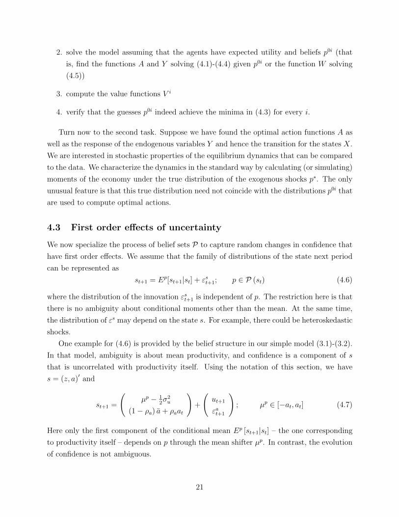
4.3 First order effects of uncertainty

We now specialize the process of belief sets P to capture random changes in confidence that

have first order effects. We assume that the family of distributions of the state next period

can be represented as

st+1 = Ep[st+1|st] + εst+1; p ∈ P (st) (4.6)

where the distribution of the innovation εst+1 is independent of p. The restriction here is that

there is no ambiguity about conditional moments other than the mean. At the same time,

the distribution of εs may depend on the state s. For example, there could be heteroskedastic

shocks.

One example for (4.6) is provided by the belief structure in our simple model (3.1)-(3.2).

In that model, ambiguity is about mean productivity, and confidence is a component of s

that is uncorrelated with productivity itself. Using the notation of this section, we have

s = (z, a)′ and

st+1 =

(µp − 1

2σ2u

(1− ρa) a+ ρaat

)+

(ut+1

εat+1

); µp ∈ [−at, at] (4.7)

Here only the first component of the conditional mean Ep [st+1|st] – the one corresponding

to productivity itself – depends on p through the mean shifter µp. In contrast, the evolution

of confidence is not ambiguous.

21

The example suggests a way to specify simple but rich families of beliefs that are

compatible with (4.6). Start from a vector u of fundamental shocks that people feel

ambiguous about. In addition to productivity, this set might contain policy shocks. Next,

define subvector a of s that has the same length as u to capture confidence about u. Finally,

parametrize the set of beliefs by an interval for each fundamental shock, centered at zero

and bounded by |a|. In principle confidence could be different for different fundamental

shocks. One could imagine, for example, that ambiguity about fiscal and monetary policy is

correlated, but quite different from ambiguity about technology. This is because the flow of

news that drives confidence is likely to be different for those shocks.

Risk shocks and ambiguity

While the simple model is homoskedastic, we emphasize that (4.6) also allows for

nonlinear specifications that link changes in ambiguity and changes in volatility. For example,

consider a variation on (4.7) with stochastic volatility in productivity that feeds back to

agents’ perception of ambiguity. Let s =(z, σ2

z,t

)st+1 =

(µp − 1

2σ2z,t

(1− ρσ) σ2z + ρσσ

2z,t

)+

(σz,tε

zt+1

εσt+1

); Rp

t =(µp)2

2σ2z,t

≤ η

where the parameters of the stochastic volatility process are chosen such that the variance

“almost never” becomes negative. With normal distributions, Rpt represents the entropy of a

belief with mean µp relative to a benchmark belief with mean zero. The inequality says that

in periods of high turbulence (high σ2z,t), there is also more ambiguity about the conditional

mean, reflected in a wider interval for that parameter.

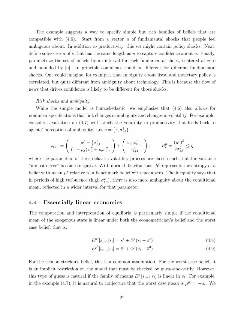
4.4 Essentially linear economies

The computation and interpretation of equilibria is particularly simple if the conditional

mean of the exogenous state is linear under both the econometrician’s belief and the worst

case belief, that is,

Ep∗ [st+1|st] = s∗ + Φ∗(st − s∗) (4.8)

Ep0

[st+1|st] = s0 + Φ0(st − s0) (4.9)

For the econometrician’s belief, this is a common assumption. For the worst case belief, it

is an implicit restriction on the model that must be checked by guess-and-verify. However,

this type of guess is natural if the family of means Ep [st+1|st] is linear in st. For example,

in the example (4.7), it is natural to conjecture that the worst case mean is µp0 = −at. We

22

now describe how the above guess-and-verify method works and how the equilibrium can be

analyzed if (4.9) holds.

Finding the equilibrium law of motion

For a given belief p0, step 2 of the procedure – finding the equilibrium law of motion –

amounts to finding a solution W (w, s) to (4.5). We look for an approximate solution by

linearization. Define the worst case steady state w by

H(w0, w0, w0, s0, s0

)= 0

Intuitively, this is where w would converge if the law of motion of the exogenous state were

(4.6) with the worst case conditional mean (4.9). The actual law of motion will typically

be different if the true conditional mean differs from the worst case. The worst case steady

state, just like the worst case belief, should be viewed only as a tool to describe agents’

responses to uncertainty.

Denote the deviation from the worst case steady state by w0t := wt− w0 and s0

t := st− s0

and perform a first order Taylor expansion of H in (4.5) around the worst case steady state

to obtain

Ep0 [α−1w

0t−1 + α0w

0t + α1w

0t+1 + δ0s

0t + δ1s

0t+1|st

]= 0 (4.10)

Together with the second equation in (4.9), this is a familiar system of expectational

difference equations. We use time subscripts to make the notation comparable to other

such equations in the literature (see for example Christiano (2002)). The timing is that

wt−1 contains endogenous variables determined one period before the exogenous state st is

realized and wt corresponds to W (wt−1, st), determined once st is known.

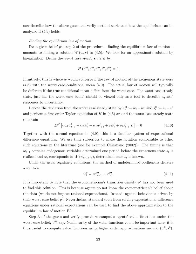
Under the usual regularity conditions, the method of undetermined coefficients delivers

a solution

w0t = ρw0

t−1 + νs0t . (4.11)

It is important to note that the econometrician’s transition density p∗ has not been used

to find this solution. This is because agents do not know the econometrician’s belief about

the data (we do not impose rational expectations). Instead, agents’ behavior is driven by

their worst case belief p0. Nevertheless, standard tools from solving expectational difference

equations under rational expectations can be used to find the above approximation to the

equilibrium law of motion W .

Step 3 of the guess-and-verify procedure computes agents’ value functions under the

worst case belief, V 0i say. Nonlinearity of the value functions could be important here; it is

thus useful to compute value functions using higher order approximations around (w0, s0).

23

Finally, step 4 verifies the guess by solving the minimization problem in (4.2) for the mean

Ep. In our applications, this amounts to checking monotonicity of a function. Indeed,

suppose beliefs are given by (4.7) and the guess is µp = Ep0 [zt+1|st] = −at. It is verified by

checking whether for any X,A, s = (z, a) and a′, the function

V (z′) := V 0(x′ (X,A, Y (X, s) , s, z′, a′) , z′, a′)

is strictly increasing.

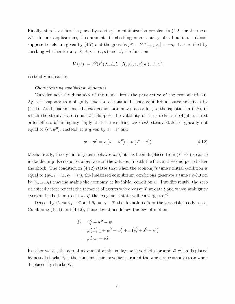
Characterizing equilibrium dynamics

Consider now the dynamics of the model from the perspective of the econometrician.

Agents’ response to ambiguity leads to actions and hence equilibrium outcomes given by

(4.11). At the same time, the exogenous state moves according to the equation in (4.8), in

which the steady state equals s∗. Suppose the volatility of the shocks is negligible. First

order effects of ambiguity imply that the resulting zero risk steady state is typically not

equal to (s0, w0). Instead, it is given by s = s∗ and

w − w0 = ρ(w − w0

)+ ν

(s∗ − s0

)(4.12)

Mechanically, the dynamic system behaves as if it has been displaced from (s0, w0) so as to

make the impulse response of wt take on the value w in both the first and second period after

the shock. The condition in (4.12) states that when the economy’s time t initial condition is

equal to (wt−1 = w, st = s∗), the linearized equilibrium conditions generate a time t solution

W (wt−1, st) that maintains the economy at its initial condition w. Put differently, the zero

risk steady state reflects the response of agents who observe s∗ at date t and whose ambiguity

aversion leads them to act as if the exogenous state will converge to s0.

Denote by wt := wt − w and st := st − s∗ the deviations from the zero risk steady state.

Combining (4.11) and (4.12), those deviations follow the law of motion

wt = w0t + w0 − w

= ρ(w0t−1 + w0 − w

)+ ν

(s0t + s0 − s∗

)= ρwt−1 + νst

In other words, the actual movement of the endogenous variables around w when displaced

by actual shocks st is the same as their movement around the worst case steady state when

displaced by shocks s0t .

24

5 An estimated model with ambiguity

This section describes the model that we use to describe the US business cycles. The model

is based on a standard medium scale DSGE model along the lines of Christiano et al. (2005)

and Smets and Wouters (2007).7 The key difference in our model is that decision makers

are ambiguity averse. We now describe the model structure and the shocks.

5.1 The model

5.1.1 The goods sector

The final output in this economy is produced by a representative final good firm that

combines a continuum of intermediate goods Yj,t in the unit interval by using the following

linear homogeneous technology:

Yt =

[∫ 1

0

Yj,t1

λf,t dj

]λf,t,

where λf,t is the markup of price over marginal cost for intermediate goods firms. The

markup shock evolves as:

log(λf,t/λf ) = ρλf log(λf,t−1/λf ) + λxf,t,

where λxf,t is i.i.d.N(0, σ2λf

). Profit maximization and the zero profit condition leads to to

the following demand function for good j:

Yj,t = Yt

(PtPj,t

) λf,tλf,t−1

(5.1)

The price of final goods is:

Pt =

[∫ 1

0

P1

1−λf,tj,t dj

](1−λf,t)

.

The intermediate good j is produced by a price-setting monopolist using the following

production function:

Yj,t = max{ZtKαj,t (εtHj,t)

1−α − Φε∗t , 0},

where Φ is a fixed cost and Kj,t and Hj,t denote the services of capital and homogeneous

7The elements characterizing the rational expectations version of our model are relatively standard inthe current literature on estimated medium-scale DSGE models (as for example in Del Negro et al. (2007),Christiano et al. (2008), Schmitt-Grohe and Uribe (2008) and Justiniano et al. (2011)).

25

labor employed by firm j. Φ is chosen so that steady state profits are equal to zero. The

intermediate goods firms are competive in factor markets, where they confront a rental rate,

Ptrkt , on capital services and a wage rate, Wt, on labor services.

The variable εt is a shock to technology, which has a covariance stationary growth rate.

The variable Zt is a stationary shock to technology. The fixed costs are modeled as growing

with the exogenous variable, ε∗t :

ε∗t = εtΥ( α

1−α t)

with Υ > 1. If fixed costs were not growing, then they would eventually become irrelevant.

We specify that they grow at the same rate as ε∗t , which is the rate at which equilibrium

output grows. Note that the growth of ε∗t , i.e. µ∗ε,t ≡ ∆ log(ε∗t ), exceeds that of εt, i.e.

µε,t ≡ ∆ log(εt) :

µ∗ε,t = µε,tΥα

1−α .

This is because we have another source of growth in this economy, in addition to the upward

drift in εt. In particular, we posit a trend increase in the efficiency of investment. We discuss

this process as well as the time series representation for the the transitory technology shock

further below. The process for the stochastic growth rate is:

log(µ∗ε,t) = (1− ρµ∗ε ) log µ∗ε + ρµ∗ε log µ∗ε,t−1 + µx∗ε,t,

where µx∗ε,t is i.i.d.N(0, σ2µ∗ε

).

We now describe the intermediate good firms pricing opportunities. Following Calvo

(1983), a fraction 1− ξp, randomly chosen, of these firms are permitted to reoptimize their

price every period. The other fraction ξp cannot reoptimize and set Pit = πPi,t−1, where π

is steady state inflation. The jth firm that has the opportunity to reoptimize its price does

so to maximize the expected present discounted value of the future profits:

Ep0

t

∞∑s=0

(βξp)s λt+sλt

[Pj,t+sYj,t+s −Wt+sHj,t+s − Pt+srkt+sKj,t+s

], (5.2)

subject to the demand function (5.1), where λt is the marginal utility of nominal income for

the representative household that owns the firm.

It should be noted that the expectation operator in these equations is, in the notation of

the general representation in section 4, the expectation under the worst case belief p0. This

is because state prices in the economy reflect ambiguity. We will describe the household’s

problem further below.

We now describe the problem of the perfectly competitive “employment agencies”. The

26

households specialized labor inputs hi,t are aggregated by these agencies into a homogeneous

labor service according to the following function:

Ht =

[∫ 1

0

(hi,t)1λw di

]λw,

where λw is the constant markup of wages over the household’s marginal rate of substitution.

These employment agencies rent the homogeneous labor service Ht to the intermediate goods

firms at the wage rate Wt. In turn, these agencies pay the wage Wi,t to the household

supplying labor of type i. Similarly as for the final goods producers, the profit maximization

and the zero profit condition leads to to the following demand function for labor input of

type i:

hi,t = Ht

(Wt

Wi,t

) λwλw−1

. (5.3)

We follow Erceg et al. (2000) and assume that the household is a monopolist in the supply

of labor by providing hi,t and it sets its nominal wage rate, Wi,t. It does so optimally with

probability 1 − ξw and with probability ξw is does not reoptimize its wage. In case it does

not reoptimize, it sets the wage as:

Wi,t = πµ∗εWi,t−1,

where µ∗ε is the steady state growth rate of the economy. When household i has the chance

to reoptimize, it does so by maximizing the expected present discounted value of future net

utility gains of working:

Ep0

t

∞∑s=0

(βξw)s[λt+sWi,t+shi,t+s −

ψL1 + σL

h1+σLi,t+s

]. (5.4)

subject to the demand function (5.3).

5.1.2 Households

The model described here is a special case of the general formulation of recursive multiple

priors of section 4. In particular, recall the recursive representation in (2.1), where preferences

are defined over uncertain streams of consumption−→C =

(−→C t

)∞t=0

, where−→C t : St → <n and

n is the number of goods. In the model described here, the consumption bundle−→C t includes

two goods: the consumption of the final good Yt and leisure. We then only have to define

27

the per-period felicity function, which for agent i is:

ui(−→C t

)= log(Ct − θCt−1)− ψL

1 + σLh1+σLi,t . (5.5)

Here Ct denotes individual consumption of the final good, hi,t denotes a specialized labor

service supplied by the household and θ is a parameter controlling internal habit formation

in consumption.8 Also, ψL > 0 is a parameter.

Utility follows a recursion similar to (2.1):

Ut

(−→C ; st

)= ui

(−→C t,−→C t−1

)+ β min

p∈Pt(st)Ep[Ut+1

(−→C ; st, st+1

)], (5.6)

Let the solution to the minimization problem in (5.6) be denoted by p0. This minimizing p0

is the same object that appears in the expectation operator of equations (5.4) and (5.2).

The type of Knightian uncertainty we consider in this model is over the transitory

technology level. In section 5.1.1, we described the production side of the economy and

showed where technology enters this economy. Ambiguity here is reflected by the set of one-

step ahead conditional beliefs Pt (st) about the future transitory technology. We follow the

description in section 4 to describe the stochastic process. Specifically, we will assume that

there is time-varying ambiguity about the future technology. This time-variation is captured

by an exogenous component at. The econometrician’s representation of the dynamics of the

transitory productivity shock Zt is the AR(1) process:

logZt = ρz logZt−1 + σzzxt . (5.7)

The set Pt of one step conditional beliefs about future technology can then be represented

by the family of processes:

logZt+1 = ρz logZt + σzzxt+1 + µt (5.8)

µt ∈ [−at,−at + 2|at|] (5.9)

at+1 = (1− ρa) a+ ρaat + σaaxt+1 (5.10)

where the shocks zx and ax are standard normal iid shocks. As in Section 4, we assume that

the agent knows the evolution of at, but that he is not sure whether the conditional mean of

logZt+1 is really ρz logZt. Instead, the agent allows for a range of intercepts. If at is higher,

then the agent is less confident about the mean of logZt+1 – his belief set is larger.

8Note that Ct is not indexed by i because we assume the existence of state contingent securities whichimplies that in equilibrium consumption and asset holdings are identical across households.

28

In this model, it is easy to see what is the worst case scenario, i.e. what is the belief

about µt that solves the minimization problem in (5.6). In section 4.4 we described a general

procedure to find the worst case belief. In the present model, the environment (given by

B, x′ u and G in the general formulation of section 4) is such that, under expected utility

and rational expectations, a first order solution provides a satisfactory approximation to

the equilibrium dynamics. In this environment, it is easy to check that the value function,

under expected utility, is increasing in Zt. This monotonicity implies that the worst case

scenario belief that solves the minimization problem in (5.6) is given by the lower bound of

the set [−at,−at + 2|at|]. Intuitively, it is natural that the agents take into account that the

worst case is always that the mean of productivity innovations is as low as possible. Thus,

according to the worst case belief p0 :

logZt+1 = ρz logZt + σzzxt+1 − at (5.11)

and the expectational operator Ep0

t denotes the expectation conditional on time t informa-

tion, which includes the belief about future Zt+1 given by (5.11).

The household accumulates capital subject to the following technology:

Kt+1 = (1− δ)Kt +

[1− S

(ζt

ItIt−1

)]It, (5.12)

where ζt is a disturbance to the marginal efficiency of investment with mean unity, Kt is the

beginning of period t physical stock of capital, and It is period t investment. The function S

reflects adjustment costs in investment. The function S is convex, with steady state values

of S = S ′ = 0, S ′′ > 0. The specific functional form for S(.) that we use is:

S

(ζt

ItIt−1

)= exp

[√S ′′

2

(ζt

ItIt−1

− 1

)]+ exp

[−√S ′′

2

(ζt

ItIt−1

− 1

)]− 2 (5.13)

The marginal efficiency of investment follows the process:

log(ζt) = ρζ log(ζt−1) + ζxt ,

where ζxt is i.i.d.N(0, σ2ζ ).

Households own the physical stock of capital and rent out capital services, Kt, to a

competitive capital market at the rate Ptrkt , by selecting the capital utilization rate ut:

Kt = utKt,

29

Increased utilization requires increased maintenance costs in terms of investment goods per

unit of physical capital measured by the function a (ut) . The function a(.) is increasing and

convex, a (1) = 0 and ut is unity in the nonstochastic steady state. We assume that a′′ (u) =

ϑrk, where rk is the steady state value of the rental rate of capital. Then, a′′ (u) /a′ (u) = ϑ

is a parameter that controls the degree of convexity of utilization costs. In the linearized

equilibrium, it is only the value ϑ that matters for dynamics. The specific functional form

for a (ut) that we use is

a(ut) =1

2rkϑu2

t + rk(1− ϑ)ut + rk(1

2ϑ− 1) (5.14)

The ith household’s budget constraint is:

PtCt + PtIt

µΥ,tΥt+Bt = Bt−1Rt−1 + PtKt[r

kt ut − a(ut)Υ

−t] +Wi,thi,t − TtPt (5.15)

where Bt are holdings of government bonds, Rt is the gross nominal interest rate and Tt is

net lump-sum taxes.

When we specify the budget constraint, we will assume that the cost, in consumption

units, of one unit of investment goods, is (ΥtµΥ,t)−1. Since the currency price of consumption

goods is Pt, the currency price of a unit of investment goods is therefore, Pt (ΥtµΥ,t)−1. The

stationary component of the relative price of investment follows the process:

log(µΥ,t/µΥ) = ρµΥlog(µΥ,t−1/µΥ) + µxΥ,t,

where µxΥ,t is i.i.d.N(0, σ2µΥ

).

5.1.3 The government

The market clearing condition for this economy is:

Ct +It

µΥ,tΥt+Gt = Y G

t (5.16)

where Gt denotes government expenditures and Y Gt is our definition of measured GDP, i.e.

Y Gt ≡ Yt − a(ut)Υ

−tKt. We model government expenditures as Gt = gtε∗t , where gt is a

stationary stochastic process. This way of modeling Gt helps to ensure that the model has a

balanced growth path. The fiscal policy is Ricardian. The government finances Gt by issuing

30

short term bonds Bt and adjusting lump sum taxes Tt. The law of motion for gt is:

log(gt/g) = ρg log(gt−1/g) + gxt

where gxt is.i.d.N(0, σ2g).

The nominal interest rate Rt is set by a monetary policy authority according to the

following feedback rule:

Rt

R=

(Rt−1

R

)ρR [(πtπ

)aπ (Y Gt

Y ∗t

)ay ( Y Gt

µ∗εYGt−1

)agy]1−ρR

exp(εR.t),

where εR.t is a monetary policy shock i.i.d.N(0, σ2εR

), π is the constant inflation target, R is

the steady state nominal interest rate target equal to πµ∗ε/β and Y ∗t is the level of output

along the deterministic growth path.

5.1.4 Parameterized ambiguity process

The laws of motion in (5.8) and (5.10) are linear. To maintain the interpretation that µt is

the worst case scenario solution to the minimization problem, at should be positive. Thus,

it is useful not to have at become negative very often. We are then guided to parameterize

the ambiguity process in the following way. We compute the unconditional variance of the

process in (5.10) and insist that the mean level of ambiguity is high enough so that even a

large negative shock to at of m unconditional standard deviations away from the mean will

remain in the positive domain. We can write this constraint as:

a ≥ mσa√

1− ρ2a

. (5.17)

The second constraint on the at process is given by the discipline argument that puts an

upper bound on the amount of ambiguity. In section 3.4 we argued that this upper bound

is equal to 2√ρσz, where ρ ∈ [0, 1] is the share of the variability in the data that agents

attribute to ambiguity. When ρ = 1 we obtain the largest upper bound, i.e. at ≤ 2σz. Then,

a similar argument as for the lower bound in (5.17) leads us to consider a process for at such

that a realization which is higher by m unconditional standard deviations than the mean is

still below this upper bound:

a+mσa√

1− ρ2a

≤ 2σz (5.18)

In preliminary estimations of the model, we find that the constraint in (5.17) between the

31

amount of unconditional volatility and mean ambiguity is binding.9 When that constraint

holds with equality it means that we can estimate two parameters out of the three: a, σa

and ρa. Notice also that in that case, the constraint in (5.18) implies that

a ≤ σz. (5.19)

For computational reasons, we choose to work with the following scaling between the mean

amount of ambiguity and the standard deviation of the technology shock:

a = nσz (5.20)

where (5.19) implies that n ∈ [0, 1]. Given this scaling, the binding constraint in (5.17)

implies that:

σa = nσz

√1− ρ2

a

m(5.21)

We fix m = 3 so that a negative shock of three unconditional standard deviations is still

in the positive domain and a positive shock of three unconditional standard deviations will

still be below the upper bound of ambiguity given by 2σz. So, the structural ambiguity

parameters to be estimated are n and ρa. Based on the estimated σz and n, we find a from

(5.20). Then using the estimated ρa we get the implied σa from (5.21).

Alternatively, instead of the scaling in (5.20), we could estimate directly the parameters

ρa and σa. The mean ambiguity would then be given by the binding constraint in (5.17). We

find that the results are very robust to this choice. An advantage of the scaling in (5.20) is

that it shows a direct link between how much ambiguity there is about the mean innovation

σzzxt and the standard deviation of that innovation. Another advantage is that the parameter

n belongs to the unit interval which is computationally convenient.

5.1.5 Model Solution

The model economy fluctuates along a stochastic growth path. Some variables are station-

ary: the nominal interest rates, the long-term interest rate, inflation and hours worked.

Consumption, real wages and output grow at the rate determined by ε∗t . The capital stock

and investment grow faster, due to increasing efficiency in the investment producing sector,

at a rate determined by ε∗tΥt, with Υ > 1.

9More precisely, if the three parameters characterizing ambiguity are separately estimated we find that theimplied unconditional volatility of the at process is so large that it implies very frequent negative realizationsto at. Additionally there are further issues of identification: if we do not fix other structural parameters, suchas β, we can easily run into identification problems of a. This is a further reason to impose a relationshipbetween the ambiguity parameters.

32

The solution of our model with ambiguity follows the general steps described in section

4.4. The solution builds on the standard approach to solve for a rational expectations

equilibrium. The difference here is that we need to take into account that the worst case

scenario expectations do not materialize on average ex-post. Therefore, the solution involves

the following procedure. First, we solve the model as a rational expectations model in

which the worst case scenario expectations are correct on average. The equations describing

the equilibrium conditions under these expectations are presented in the Appendix 6.1. To

solve for the equilibrium, we follow the standard approach in the literature: we rewrite the

model in terms of stationary variables by detrending each variable using its specific trend

growth rate. Then we find the non-stochastic steady state for this detrended system and

construct a log-linear approximation around it. We then solve the resulting linear system of

rational expectations equations. Second, we take the equilibrium decision rules formed under

ambiguity and then characterize the dynamics under the econometrician’s law of motion for

the productivity process described in equation (5.7). Details of the solution method are

available in Appendix 6.2.

5.1.6 Estimation and Data

The linearity of the state space representation of the model and the assumed normality of

the shocks allow us to estimate the model using standard Bayesian methods as discussed

for example in An and Schorfheide (2007) and Smets and Wouters (2007). We estimate the

posterior distribution of the structural parameters by combining the likelihood function with

prior information. The likelihood is based on the following vector of observable variables:

[∆ log Y G

t ,∆ log It,∆ logCt, logLt, log πt, logRt,∆ logPI,t]

where ∆ denotes the first difference operator. The vector of observables refers to data for

US on GDP growth rate, investment growth rate, consumption growth rate, log of hours per

capita, log of gross inflation rate, log of gross short term nominal interest rate and price of

investment growth rate. The sample period used in the estimation is 1984Q1-2010Q1. The

data sources are described in Appendix 6.3. In the state space representation we do not

allow for a measurement error on any of the observables.

We now discuss the priors on the structural parameters. The only parameter we calibrate

is the share of government expenditures in output which is set to match the observed

empirical ratio of 0.22. The rest of the structural parameters are estimated. The priors on

the parameters not related to ambiguity and thus already present in the standard medium

scale DSGE are broadly in line with those adopted in previous studies (e.g. Christiano et al.

33

(2010b) and Justiniano et al. (2011)). The prior for each of the autocorrelation parameter

of the shock processes is a Beta distribution with a mean of 0.5 and a standard deviation

of 0.15. The prior distribution for the standard deviation of the 7 fundamental shocks is an

Inverse Gamma with a mean of 0.01 and a standard deviation of 0.01.

Regarding the ambiguity parameters, we follow the argument in section 5.1.4 and estimate

the two parameters n and ρa. The prior on the scaling parameter n is a Beta distribution

with mean 0.5 and standard deviation equal to 0.25. The prior is loose and it allows a wide

range of plausible values. The prior on ρa follows the pattern of the other autocorrelation

coefficients and is a Beta distribution with a mean of 0.5 and a standard deviation of 0.15.

The prior and posterior distributions are described in Table 2. The posterior estimates

of our structural parameters that are unrelated to ambiguity are in line with previous

estimations of such medium scale DSGE models (Del Negro et al. (2007), Smets and Wouters

(2007), Justiniano et al. (2011), Christiano et al. (2010b)). These parameters imply that

there are significant ‘frictions’ in our model: price and wage stickiness, investment adjustment

costs and internal habit formation are all substantial. The estimated policy rule is inertial

and responds strongly to inflation but also to output gap and output growth. Given that

these parameters have been extensively analyzed in the literature, we now turn attention to

the role of ambiguity in our estimated model.

5.2 Results

We evaluate the importance of ambiguity in our model along two dimensions: the steady

state effect of ambiguity and its role in business cycle fluctuations. We will argue that

ambiguity plays an important part along both of these dimensions.

5.2.1 Steady state

The posterior mode of the structural parameters of ambiguity implies that the steady state

level of ambiguity is

a = nσz = 0.963× 0.0045 = 0.00435

which implies that the agent is on average concerned about a one-step ahead future technol-

ogy level that is 0.435% lower than the true technology, normalized to 1. In the long run,

the agent expects the technology level to be Z∗, which solves:

logZ∗ = ρz logZ∗ − a.

34

For the estimated ρz = 0.955, we get that Z∗ = 0.903. Thus, the ambiguity-averse agent

expects under his worst case scenario evaluation the long run mean technology to be

approximately 9% lower than the true mean. Based on these estimates and using (5.17) we

can directly find that the standard deviation of the innovations to ambiguity is σa = 0.000405.

Our interpretation of the reason why we find a relatively large a is the following: the

estimation prefers to have a large σa because the ambiguity shock provides a channel in the

model that delivers dynamics that seem to be favored by the data. Indeed, as detailed in

the next section, the ambiguity shocks generate comovement between variables that enter in

the observation equation. This is a feature that is strongly present in the data and is not

easily captured by other shocks. Given the large role that the fit of the data places on the

ambiguity shock, the implied estimated σa is relatively large. Because of the constraint on

the size of the mean ambiguity in (5.17), this results also in a large required steady state

ambiguity. Thus, given also the estimated σz, the posterior mode for n is relatively large.

The picture that comes out of these estimates is that ambiguity is large in the steady state,

it is volatile and persistent.

The estimated amount of ambiguity has substantial effects on the steady state of en-

dogenous variables.10 To describe these effects we perform the following calculations.11

We fix all the estimated parameters of the model at their posterior mode but change

the standard deviation of the transitory technology shock, σz, from its estimated value

of σz = 0.0045 to being equal to 0. When σz = 0, then the level of ambiguity a is also

equal to 0.12 By reporting the difference between the steady states with σz = σz > 0 and

with σz = 0 we calculate the steady state effect of fluctuations in transitory technology that

goes through the estimated amount of ambiguity. In Table 1 we present the net percent

difference of some variables of interest between the two cases, i.e. for a variable X we report

100[XSS, (σz = σz)/XSS, (σz = 0) − 1], where XSS, (σz = σz) and XSS, (σz = 0) are the

steady states of variable X under σz = σz and respectively σz = 0.13

As evident from Table 1, the effect of fluctuations in the transitory technology shock

that goes through ambiguity is very substantial. Output, capital, consumption, hours are all

significantly smaller, by about 15%, when σz = σz. The nominal interest rate is smaller by

10As described in Section 4.4, we refer to the steady state of our linearized model as a ‘zero risk steadystate’, in which the variances of the shocks only have an effect on the endogenous variables through ambiguity.

11The quantitative implications of the model are reported by evaluating the parameters at their posteriormode.

12As evident from equation (5.18) or from the discussion of Section 3.4, since 0 ≤ a ≤ σz, then σz = 0implies a = 0. Intuitively, when there is no observed variability in the zt process, then there cannot be anyperceived ambiguity about its one-step ahead mean.

13Note that for welfare, we report the difference between WelfSS,(σz=σz) and WelfSS,(σz=0) in terms ofsteady state consumption under σz = 0.

35

Table 1: Steady state percent difference from zero fluctuations

Variable Welfare Output Capital Consumption Hours Nom.Rate

-13.1 -15 -14 -16.4 -14.8 -42.5

42%, which corresponds to the quarterly steady state interest rate being lower by 73 basis

points. Importantly, the welfare cost of fluctuations in this economy is also very large, of

about 13% of steady state consumption.

The steady state effects of fluctuations in technology that go through ambiguity are much

larger than what it is implied by the standard analysis featuring only risk. By standard

analysis we mean the strategy of shutting down all the other shocks except the transitory

technology and computing a second order approximation of the model in which there is no

ambiguity but σz = σz. For such a calculation, we find that the welfare cost of business cycle

fluctuations is around 0.01% of steady state consumption. The effects on the steady state

values of the other variables reported in Table 1 is negligible. This latter result is consistent

with the conclusions of the literature on the effect of business cycle fluctuations and risk, as

in Lucas (1987).

5.2.2 Business cycle fluctuations

In this section we analyze the role of time-varying ambiguity in generating business cycles.

We highlight the role of ambiguity by discussing three main points: a theoretical variance

decomposition of variables; a historical variance decomposition based on the smoothed shocks

and impulse responses experiments.

Variance decomposition Table 3 reports the theoretical variance decomposition of sev-

eral variables of interest. For each structural shock we compute the share of the total

variation in the corresponding variable that is accounted by that shock at two horizons:

one is at the business cycle frequency which incorporates periodic components with cycles

between 6 and 32 quarters, as in Stock and Watson (1999). The second is at a long-run

horizon which is the theoretical variance decomposition obtained by solving the dynamic

Lyapunov equation characterizing the law of motion of the model. These two shares are

reported in the first two rows of Table 3. In the third row, we also report for comparison

the variance decomposition in an estimated model without ambiguity.

The main message of this exercise is that ambiguity shocks can be a very influential factor

in explaining the variance of key economic variables. At business cycle frequency this shock

36

accounts for about 27% of GDP variability and it simultaneously explains a large share of real

variables such as consumption (52%), investment (14%), hours (31%) and less for inflation

(2%) and the nominal interest rate (7%). The long-run theoretical decomposition implies

that the shock is even more important. It explains about 55% of GDP variability and it is

a very significant driver of the rest of the variables: consumption (62%), investment (51%),

hours (52%), inflation (29%) and the nominal interest rate (38%). Based on these two sets of

numbers we can conclude that the ambiguity shock is an important driver of business cycle

fluctuations while also having a low-frequency component that magnifies its role in the total

variance decomposition. The simultaneous large shares of variation explained by ambiguity

suggest that time-variation in the confidence of the agents about transitory technology shocks

can be a unified source of macroeconomic variability.

For comparison, we can analyze the estimated model without ambiguity. The business

cycle frequency variance decomposition for a model that sets the level of ambiguity to zero,

i.e. n = 0, is reported in the third row of Table 3. There the largest share of GDP variability

is explained by the marginal efficiency of investment shock, confirming the results of many

recent studies, such as Christiano et al. (2010b) and Justiniano et al. (2011). Introducing

time-varying ambiguity reduces the importance of the other shocks, except for the transitory

technology shock Zt, in explaining the decomposition of the level of observed variables. The

reduction in effects are especially strong for the marginal efficiency of investment and growth

rate shocks. With ambiguity, the shock Zt becomes more important. The reason is that

ambiguity enters in the model indirectly through the variance of σz. Thus, with ambiguity

the estimated variance of Zt affects the likelihood evaluation through two channels: one

direct, through the shock Zt, and one indirect through the variance of the shock at.

Impulse response We now turn to analyzing the impulse responses for the ambiguity

shock in the estimated model. As suggested already in the discussion, an increase in

ambiguity generates a recession, in which hours worked, consumption and investment fall.

It is also worth emphasizing that the impulse response is symmetric: a fall in ambiguity,

compared to steady state, generates an economic boom in which variables comove positively.

The fact that this shock predicts comovement between this variables is an important feature

that helps explain why the estimation prefers in the likelihood maximization such a shock.

Before we proceed further, let us define the excess return on capital. The return on

capital RKt is defined in equation (6.9) in Appendix. The ex-post excess return ext+1 is then

defined as the difference between the realized return on capital and the nominal interest rate,

i.e. ext+1 := RKt+1 − Rt. As detailed in Appendix, from the two intertemporal optimality

conditions with respect to capital and bonds, it follows that in the linearized equilibrium,

37

Rt equals Ep0

t RKt+1. Thus, under the worst case expectations, Ep0

t ext+1 = 0. However, the

average realized RKt+1 will be in general different than Ep0

t RKt+1. The reason is that the former

is obtained under the true data generating process in which the worst case mean at does not

materialize on average in the realization of zt+1, while Ep0

t RKt+1 represents the average RK

t+1

if at would materialize.

Figure 3 plots the responses to a one standard deviation increase in ambiguity for the

estimated model.14 On top of the mentioned comovement in macro aggregates, the model

also predicts a fall in the price of capital, a fall in the real interest rate and a countercyclical

ex-post excess return.15

We briefly explain these results. The main intuition in understanding the effect of the

ambiguity shock is to relate it to its interpretation of a news shock. An increase in ambiguity

makes the agent act under a more cautious forecast of the future technology. From an

outside observer that analyzes the agent’s behavior, it seems that this agent acts under

some negative news about future productivity. This negative news interpretation of the

increase in ambiguity helps explain the mechanics and economics of the impulse response.

As described in detail in Christiano et al. (2008), Christiano et al. (2010a), in a rational

expectations model, a negative news about future productivity can produce a significant

bust in real economy while simultaneously generating a fall in the price of capital. This

result is reflected in our impulse response. In our model, the negative news is on average not

materialized, because nothing changed in the true process for technology, as shown in the

first panel of Figure 3. However, because of the persistent effect of ambiguity, the economy

continues to go through a prolonged recession.

The ex-post excess return, defined above as ext+1 is positive following the period of the

initial increase in ambiguity and it is positive persistently along the path. The explanation for

the countercyclical excess returns is that the negative expectation about future productivity

does not materialize in the true data generating process, so ex-post, capital pays more. Thus

along this path of higher ambiguity, RKt+1 is systematically higher than Ep0

t RKt+1. The ex-post

excess return reflects a rational uncertainty premium that ambiguity averse agents require

to invest in the uncertain asset.

Historical shock decomposition We conclude the description of the role of ambiguity

shocks in business cycle fluctuations by discussing the historical variance decomposition and

the smoothed shocks that result from the estimated model. In Figure 1 we plot the Kalman

filter estimate of the ambiguity shock at, as a deviation from its steady state value. The figure

14The impulse response is plotted as percentage deviations from the ‘zero risk steady state’ of the model.15By price of capital we mean the Tobin’s marginal q. For the equation determining the evolution of qt in

the scaled version of our economy, see equation (6.11) in Appendix.

38

first shows that ambiguity is very persistent. After an initial increase around 1991, which

also corresponds to an economic downturn, the level of ambiguity was low and declining

during the 90’s, reaching its lowest values around 2000. It then increases back to levels close

to steady state until 2005. Following a few years of relatively small upward deviations from

its mean, ambiguity spikes starting in 2008. Ambiguity rapidly increases, so that throughout

2008 it doubles over each quarter. Ambiguity reaches its peak in 2008Q4 when it is 8 times

larger than its 2008Q1 value. The figure shows a dotted vertical line at 2008Q3, which

corresponds to the Lehman Brothers bankruptcy. Our model interprets the period following

2008Q1 as one in which ambiguity about future productivity has increased dramatically.

Based on these smoothed path of ambiguity shocks we can now calculate what the model

implies for the historical evolution of endogenous variables. In Figure 2 we compare, as

deviations from steady state, the observed data with the counterfactual historical evolution

for the growth rate of output, consumption, investment and the level of hours worked when

the ambiguity shock is the only shock active in the model economy. The ambiguity shock

implies a path for variables that comes close to matching the data, especially for output,

consumption and hours. The model implied path of investment is less volatile but the

correlation with the observed data is still significantly large. It is interesting that the

ambiguity shock helps explain some of the business cycle frequency of these variables but

also the low-frequency component as present in hours worked.16

The ambiguity shock generates the three large recessions observed in this sample. Indeed,

if we analyze the smoothed path of the shock in figure 2, the time-varying ambiguity helps

explain the recession of the 1991, the large growth of the 1990’s (as a period of low ambiguity),

and then the recession of 2001. Given that the estimated ambiguity still continues to rise

through 2005, the model misses by predicting a more prolonged recession than in the data,

where output picks up quickly. The rise in ambiguity in 2008 predicts in the model that

output, investment and consumption fall. The model matches the fall in consumption, but

fails to generate a large fall in investment. It is important to highlight that the ambiguity

shock implies that in the model consumption and investment comove. Indeed, in the

historical decomposition, recessions are times when both of these variables fall. This is an

important effect because standard shocks that have been recently found to be quantitatively

important (as for example in Christiano et al. (2010b) and Justiniano et al. (2011)), such as

the marginal efficiency of investment or intertemporal preference shocks imply a weak, and

most often a negative comovement between these two components.

Overall, we draw the conclusion that an increase in Knightian uncertainty (ambiguity)

16Usually the low-frequency movement in hours worked is attributed to exogenous labor supply shocks,corresponding to shocks to ψL in our model. See for example Justiniano et al. (2011).

39

generates in our estimated model a recession, in which consumption, investment and price of

capital fall, while producing countercyclical ex-post excess returns. Given these dynamics,

we believe that time-varying ambiguity can be an important source of observed business

cycle dynamics.

40

6 Appendix

6.1 Equilibrium conditions for the estimated model

Here we describe the equations that characterize the equilibrium of the model described in

Section 5.

To solve the model, we first scale the variables in order to induce stationarity. As

mentioned in section 5.1.1, the model has two sources of growth: a stochastic trend in

neutral technology and a deterministic trend in the price of investment goods. The real

variables are scaled as follows:

ε∗t = εtΥ( α

1−α t), ct =Ctε∗t, yt =

Ytε∗t, gt =

Gt

ε∗t

kt+1 =Kt+1

ε∗tΥt, it =

Itε∗tΥ

t, λz,t = λtPtε

∗t .

where λt is the Lagrange multiplier on the household budget constraint in (5.15). The scaling

here indicates that because of the deterministic trend in the price of investment goods, the

capital stock and investment grow at a faster rate than output and consumption.

Let µt be the Lagrange multiplier on the capital accumulation equation in (5.12) and

define the nominal price of capital expressed in units of consumption goods as

QK,t =µtλt

Price variables are then scaled as:

qt =QK,t

Υ−tPt, rkt =

rktΥ−t

, wt =Wt

ε∗tPt

We will also make use of other scaling conventions:

µ∗ε,t = µε,tΥα

1−α , p∗t = (Pt)−1

1∫0

P

λf,t1−λf,tj,t dj

1−λf,tλf,t

, w∗t = (Wt)−1

1∫0

Wλw

1−λwi,t di

1−λwλw

,

where the index i refers to households and the index j to monopolistically competitive firms.

We now present the nonlinear equilibrium conditions characterizing the model, in scaled

form. As noted in section 5, the expectation operator in these equations, Ep0

t , is the one-

step ahead conditional expectation under the worst case belief p0. The latter is described by

equation (5.11).

41

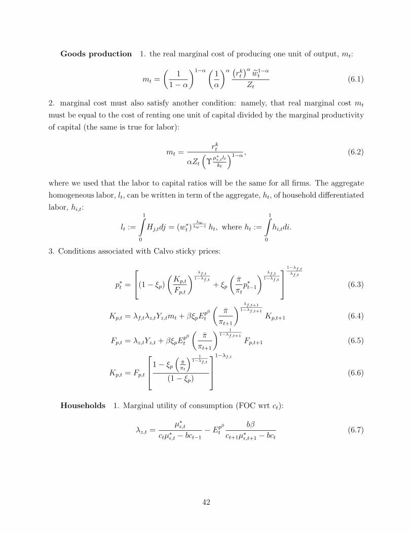
Goods production 1. the real marginal cost of producing one unit of output, mt:

mt =

(1

1− α

)1−α(1

α

)α (rkt )α w1−αt

Zt(6.1)

2. marginal cost must also satisfy another condition: namely, that real marginal cost mt

must be equal to the cost of renting one unit of capital divided by the marginal productivity

of capital (the same is true for labor):

mt =rkt

αZt

(Υµ∗ε,tlt

kt

)1−α , (6.2)

where we used that the labor to capital ratios will be the same for all firms. The aggregate

homogeneous labor, lt, can be written in term of the aggregate, ht, of household differentiated

labor, hi,t:

lt :=

1∫0

Hj,tdj = (w∗t )λwλw−1 ht, where ht :=

1∫0

hi,tdi.

3. Conditions associated with Calvo sticky prices:

p∗t =

(1− ξp)(Kp,t

Fp,t

) λf,t1−λf,t

+ ξp

(π

πtp∗t−1

) λf,t1−λf,t

1−λf,tλf,t

(6.3)

Kp,t = λf,tλz,tYz,tmt + βξpEp0

t

(π

πt+1

) λf,t+11−λf,t+1

Kp,t+1 (6.4)

Fp,t = λz,tYz,t + βξpEp0

t

(π

πt+1

) 11−λf,t+1

Fp,t+1 (6.5)

Kp,t = Fp,t

1− ξp(ππt

) 11−λf,t

(1− ξp)

1−λf,t

(6.6)

Households 1. Marginal utility of consumption (FOC wrt ct):

λz,t =µ∗ε,t

ctµ∗ε,t − bct−1

− Ep0

t

bβ

ct+1µ∗ε,t+1 − bct(6.7)

42

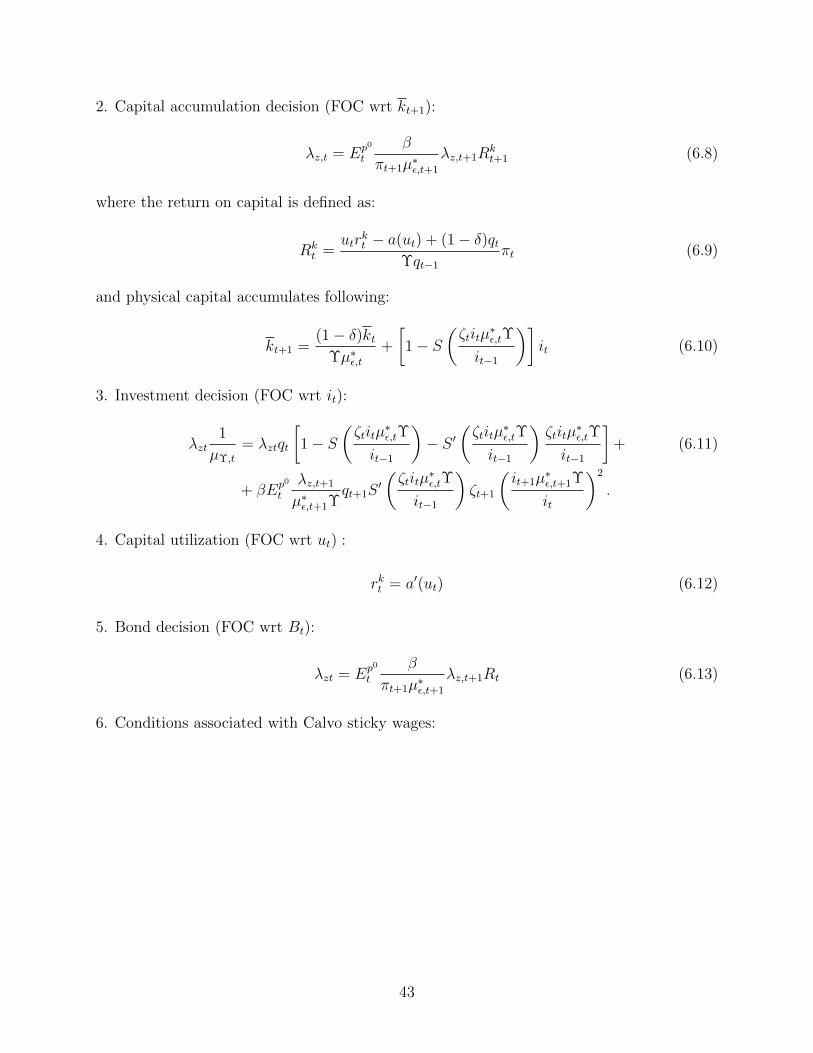
2. Capital accumulation decision (FOC wrt kt+1):

λz,t = Ep0

t

β

πt+1µ∗ε,t+1

λz,t+1Rkt+1 (6.8)

where the return on capital is defined as:

Rkt =

utrkt − a(ut) + (1− δ)qt

Υqt−1

πt (6.9)

and physical capital accumulates following:

kt+1 =(1− δ)kt

Υµ∗ε,t+

[1− S

(ζtitµ

∗ε,tΥ

it−1

)]it (6.10)

3. Investment decision (FOC wrt it):

λzt1

µΥ,t

= λztqt

[1− S

(ζtitµ

∗ε,tΥ

it−1

)− S ′

(ζtitµ

∗ε,tΥ

it−1

)ζtitµ

∗ε,tΥ

it−1

]+ (6.11)

+ βEp0

t

λz,t+1

µ∗ε,t+1Υqt+1S

′(ζtitµ

∗ε,tΥ

it−1

)ζt+1

(it+1µ

∗ε,t+1Υ

it

)2

.

4. Capital utilization (FOC wrt ut) :

rkt = a′(ut) (6.12)

5. Bond decision (FOC wrt Bt):

λzt = Ep0

t

β

πt+1µ∗ε,t+1

λz,t+1Rt (6.13)

6. Conditions associated with Calvo sticky wages:

43

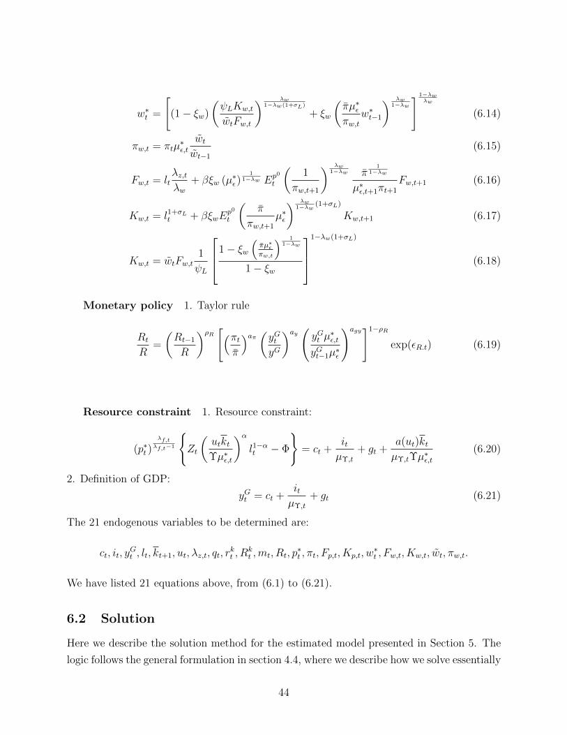
w∗t =

[(1− ξw)

(ψLKw,t

wtFw,t

) λw1−λw(1+σL)

+ ξw

(πµ∗επw,t

w∗t−1

) λw1−λw

] 1−λwλw

(6.14)

πw,t = πtµ∗ε,t

wtwt−1

(6.15)

Fw,t = ltλz,tλw

+ βξw (µ∗ε)1

1−λw Ep0

t

(1

πw,t+1

) λw1−λw π

11−λw

µ∗ε,t+1πt+1

Fw,t+1 (6.16)

Kw,t = l1+σLt + βξwE

p0

t

(π

πw,t+1

µ∗ε

) λw1−λw

(1+σL)

Kw,t+1 (6.17)

Kw,t = wtFw,t1

ψL

1− ξw(πµ∗επw,t

) 11−λw

1− ξw

1−λw(1+σL)

(6.18)

Monetary policy 1. Taylor rule

Rt

R=

(Rt−1

R

)ρR [(πtπ

)aπ (yGtyG

)ay ( yGt µ∗ε,tyGt−1µ

∗ε

)agy]1−ρR

exp(εR.t) (6.19)

Resource constraint 1. Resource constraint:

(p∗t )λf,tλf,t−1

{Zt

(utktΥµ∗ε,t

)αl1−αt − Φ

}= ct +

itµΥ,t

+ gt +a(ut)ktµΥ,tΥµ∗ε,t

(6.20)

2. Definition of GDP:

yGt = ct +itµΥ,t

+ gt (6.21)

The 21 endogenous variables to be determined are:

ct, it, yGt , lt, kt+1, ut, λz,t, qt, r

kt , R

kt ,mt, Rt, p

∗t , πt, Fp,t, Kp,t, w

∗t , Fw,t, Kw,t, wt, πw,t.

We have listed 21 equations above, from (6.1) to (6.21).

6.2 Solution

Here we describe the solution method for the estimated model presented in Section 5. The

logic follows the general formulation in section 4.4, where we describe how we solve essentially

44

linear economies with ambiguity aversion.

Let wt denote the endogenous variables and st the exogenous variables. For notational

purposes, split the vector st into the technology shock zt := logZt, the ambiguity variable

at and the rest of the exogenous variables, st, expressed in logs, of size n. In the case of our

estimated model n = 6. Under the worst case belief

zt+1 = ρzzt + zxt+1 − at (6.22)

We can then summarize our procedure for finding the equilibrium dynamics in the following

steps:

1. Find the deterministic ‘worst case steady state’. Here we take the steady state values

of exogenous variables s0. This vector includes setting at = a, st = s0n×1 and finding

the steady state technology level of the process in (6.22). The latter is

zo = − a

1− ρz

Using s0 := (s0n×1, z

o, a) one can compute the ‘worst case steady state’ of the endoge-

nous variables. This can be done by analytically solving the equilibrium conditions

presented in section 6.1 evaluated at a deterministic steady state s0. Denote these

steady state values of these endogenous variables as a vector w0m×1.

2. Linearize the model around the ‘worst case steady state’. Denote the deviation from

the worst case steady state by w0t := wt−w0 and s0

t := st−s0. Posit a linear equilibrium

law of motion:

w0t = Aw0

t−1 +Bs0t (6.23)

and specify the linear evolution of the exogenous variables:

s0t :=

stztat

= P

st−1

zt−1

at−1

+

εt

zxt

axt

where Ξt :=

[εt zxt axt

]′denotes the innovations to the exogenous variables st with

Ξt ∼ N (0,Σ). Importantly for us,

Ep0

s0t+1 = P s0

t + Ep0

Ξt+1, (6.24)

where Ep0Ξt+1 = 0. To reflect the time t worst case belief about zt+1, recall (6.22) so

45

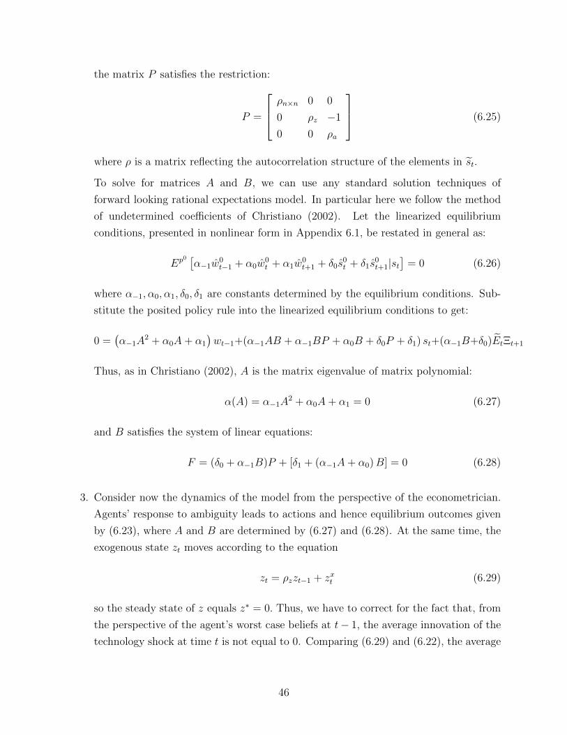
the matrix P satisfies the restriction:

P =

ρn×n 0 0

0 ρz −1

0 0 ρa

(6.25)

where ρ is a matrix reflecting the autocorrelation structure of the elements in st.

To solve for matrices A and B, we can use any standard solution techniques of

forward looking rational expectations model. In particular here we follow the method

of undetermined coefficients of Christiano (2002). Let the linearized equilibrium

conditions, presented in nonlinear form in Appendix 6.1, be restated in general as:

Ep0 [α−1w

0t−1 + α0w

0t + α1w

0t+1 + δ0s

0t + δ1s

0t+1|st

]= 0 (6.26)

where α−1, α0, α1, δ0, δ1 are constants determined by the equilibrium conditions. Sub-

stitute the posited policy rule into the linearized equilibrium conditions to get:

0 =(α−1A

2 + α0A+ α1

)wt−1+(α−1AB + α−1BP + α0B + δ0P + δ1) st+(α−1B+δ0)EtΞt+1

Thus, as in Christiano (2002), A is the matrix eigenvalue of matrix polynomial:

α(A) = α−1A2 + α0A+ α1 = 0 (6.27)

and B satisfies the system of linear equations:

F = (δ0 + α−1B)P + [δ1 + (α−1A+ α0)B] = 0 (6.28)

3. Consider now the dynamics of the model from the perspective of the econometrician.

Agents’ response to ambiguity leads to actions and hence equilibrium outcomes given

by (6.23), where A and B are determined by (6.27) and (6.28). At the same time, the

exogenous state zt moves according to the equation

zt = ρzzt−1 + zxt (6.29)

so the steady state of z equals z∗ = 0. Thus, we have to correct for the fact that, from

the perspective of the agent’s worst case beliefs at t− 1, the average innovation of the

technology shock at time t is not equal to 0. Comparing (6.29) and (6.22), the average

46

innovation is then equal to at−1 :

zt = Ep0

zt + at−1. (6.30)

(a) Find the ‘zero risk steady state’. Take the steady state of the exogenous variables

under the econometrician’s belief s∗ := (s0n×1, z

∗, a) which differs from s0 only in

the element corresponding to the steady state technology level z∗. Then, the zero

risk steady state is the fixed point w that solves

w − w0 = A(w − w0

)+B

(s∗ − s0

)(6.31)

where the difference s∗− s0 =[

0n×1 z∗ − zo 0]′. Thus, w can be analytically

found as:

w = w0 +B(s∗ − s0) (I − A)−1

(b) Dynamics around the ‘zero risk steady state’.

Denote by wt := wt− w and st := st− s∗ the deviations from the zero risk steady

state. Combining (6.23) and (6.31), those deviations follow the law of motion

wt = w0t + w0 − w

= A(w0t−1 + w0 − w

)+B

(s0t + s0 − s∗

)= Awt−1 +Bst (6.32)

We want to characterize the equilibrium dynamics under the econometrician’s

belief in which the worst case belief at−1 is not materialized in the zt realization.

That means that the law of motion for the exogenous states under the econome-

trician belief is

st =

ρn×n 0 0

0 ρz 0

0 0 ρa

st−1 + Ξt. (6.33)

As presented in equation (6.30), we can then describe this evolution by adding an

average innovation of at−1 to the expected value of zt formed under the time t− 1

worst case belief. The latter expectation is formed using the matrix P as defined

47

in (6.25), so we can write (6.33) as:

st = P st−1 +

0n×n 0 0

0 0 1

0 0 0

st−1 + Ξt (6.34)

6.3 Data sources

The data used to construct the observables are:

1. Real Gross Domestic Product, BEA, NIPA table 1.1.6, line 1, billions of USD, in 2005

chained dollars.

2. Gross Domestic Product, BEA, NIPA table 1.1.5, line 1, billions of USD, seasonally

adjusted at annual rates.

3. Personal consumption expenditures on nondurable goods, BEA, NIPA table 1.1.5, line

5, billions of USD, seasonally adjusted at annual rates

4. Personal consumption expenditures on services, BEA, NIPA table 1.1.5, line 6, billions

of USD, seasonally adjusted at annual rates

5. Gross private domestic investment, fixed investment, nonresidential and residential,

BEA, NIPA table 1.1.5, line 8, billions of USD, seasonally adjusted at annual rates

6. Personal consumption expenditures on durable goods, BEA, NIPA table 1.1.5, line 4,

billions of USD, seasonally adjusted at annual rates.

7. Nonfarm business hours worked, BLS, PRS85006033, seasonally adjusted, index 1992=100.

8. Civilian noninstitutional population over 16, BLS LNU00000000Q.

9. Effective Federal Funds Rate. Source: Board of Governors of the Federal Reserve

System.

We then perform the following transformations of the above data to get the observables:

10. GDP deflator: (2) / (1)

11. Real per capita GDP: (1) / (8)

12. Real per capita consumption: [(3)+(4)] / [(8)*(10)]

13. Real per capita investment: [(5)+(6)] / [(8)*(10)]

48

14. Per capital hours: (7) / (8)

15. Relative price of investment: We use the price index for consumption expenditures on

durable goods (BEA, NIPA table 1.1.4, line 4) and price index for fixed investment

(BEA, NIPA table 1.1.4, line 8). We follow the methodology proposed in Fisher (2006).

An appendix detailing the procedure used in the construction of this series is available

from the authors upon request.

49

References

An, S. and F. Schorfheide (2007): “Bayesian Analysis of DSGE Models,” Econometric

Reviews, 26, 113–172.

Angeletos, G. and J. La’O (2011): “Decentralization, Communication, and the Origins

of Fluctuations,” NBER Working Papers 17060.

Anscombe, F. and R. Aumann (1963): “A Definition of Subjective Probability,” Annals

of mathematical statistics, 199–205.

Arellano, C., Y. Bai, and P. Kehoe (2010): “Financial Markets and Fluctuations in

Uncertainty,” FRB of Minneapolis, Research Department Staff Report.

Bachmann, R., S. Elstner, and E. Sims (2010): “Uncertainty and Economic Activity:

Evidence from Business Survey Data,” NBER Working Papers 16143.

Barsky, R. and E. Sims (2011): “Information, Animal Spirits, and the Meaning of

Innovations in Consumer Confidence,” The American Economic Review, forthcoming.

Basu, S. and B. Bundick (2011): “Uncertainty Shocks in a Model of Effective Demand,”

Boston College Working Papers 774.

Beaudry, P. and F. Portier (2006): “Stock Prices, News, and Economic Fluctuations,”

American Economic Review, 96, 1293–1307.

Bidder, R. and M. Smith (2011): “Robust Control in a Nonlinear DSGE Model,”

Unpublished manuscript, San Francisco Fed.

Blanchard, O., J. L’Huillier, and G. Lorenzoni (2009): “News, Noise, and

Fluctuations: An Empirical Exploration,” NBER Working Papers 15015.

Bloom, N., M. Floetotto, and N. Jaimovich (2009): “Really Uncertain Business

Cycles,” Unpublished manuscript, Stanford University.

Cagetti, M., L. P. Hansen, T. Sargent, and N. Williams (2002): “Robustness and

Pricing with Uncertain Growth,” Review of Financial Studies, 15, 363–404.

Calvo, G. (1983): “Staggered Prices in a Utility-Maximizing Framework,” Journal of

monetary Economics, 12, 383–398.

Christiano, L. (2002): “Solving Dynamic Equilibrium Models by a Method of Undeter-

mined Coefficients,” Computational Economics, 20, 21–55.

50

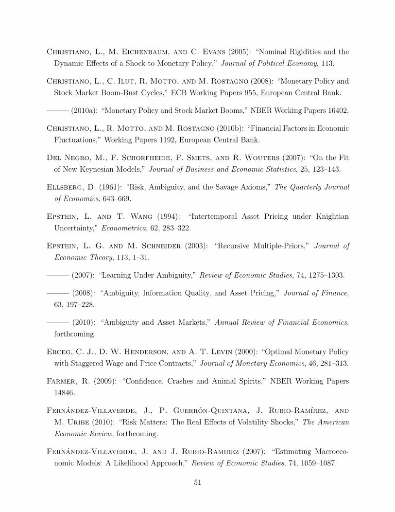
Christiano, L., M. Eichenbaum, and C. Evans (2005): “Nominal Rigidities and the

Dynamic Effects of a Shock to Monetary Policy,” Journal of Political Economy, 113.

Christiano, L., C. Ilut, R. Motto, and M. Rostagno (2008): “Monetary Policy and

Stock Market Boom-Bust Cycles,” ECB Working Papers 955, European Central Bank.

——— (2010a): “Monetary Policy and Stock Market Booms,” NBER Working Papers 16402.

Christiano, L., R. Motto, and M. Rostagno (2010b): “Financial Factors in Economic

Fluctuations,” Working Papers 1192, European Central Bank.

Del Negro, M., F. Schorfheide, F. Smets, and R. Wouters (2007): “On the Fit

of New Keynesian Models,” Journal of Business and Economic Statistics, 25, 123–143.

Ellsberg, D. (1961): “Risk, Ambiguity, and the Savage Axioms,” The Quarterly Journal

of Economics, 643–669.

Epstein, L. and T. Wang (1994): “Intertemporal Asset Pricing under Knightian

Uncertainty,” Econometrica, 62, 283–322.

Epstein, L. G. and M. Schneider (2003): “Recursive Multiple-Priors,” Journal of

Economic Theory, 113, 1–31.

——— (2007): “Learning Under Ambiguity,” Review of Economic Studies, 74, 1275–1303.

——— (2008): “Ambiguity, Information Quality, and Asset Pricing,” Journal of Finance,

63, 197–228.

——— (2010): “Ambiguity and Asset Markets,” Annual Review of Financial Economics,

forthcoming.

Erceg, C. J., D. W. Henderson, and A. T. Levin (2000): “Optimal Monetary Policy

with Staggered Wage and Price Contracts,” Journal of Monetary Economics, 46, 281–313.

Farmer, R. (2009): “Confidence, Crashes and Animal Spirits,” NBER Working Papers

14846.

Fernandez-Villaverde, J., P. Guerron-Quintana, J. Rubio-Ramırez, and

M. Uribe (2010): “Risk Matters: The Real Effects of Volatility Shocks,” The American

Economic Review, forthcoming.

Fernandez-Villaverde, J. and J. Rubio-Ramirez (2007): “Estimating Macroeco-

nomic Models: A Likelihood Approach,” Review of Economic Studies, 74, 1059–1087.

51

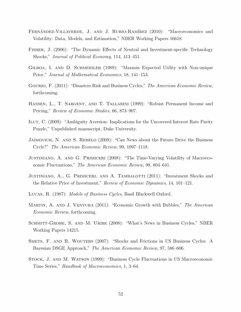
Fernandez-Villaverde, J. and J. Rubio-Ramırez (2010): “Macroeconomics and

Volatility: Data, Models, and Estimation,” NBER Working Papers 16618.

Fisher, J. (2006): “The Dynamic Effects of Neutral and Investment-specific Technology

Shocks,” Journal of Political Economy, 114, 413–451.

Gilboa, I. and D. Schmeidler (1989): “Maxmin Expected Utility with Non-unique

Prior,” Journal of Mathematical Economics, 18, 141–153.

Gourio, F. (2011): “Disasters Risk and Business Cycles,” The American Economic Review,

forthcoming.

Hansen, L., T. Sargent, and T. Tallarini (1999): “Robust Permanent Income and

Pricing,” Review of Economic Studies, 66, 873–907.

Ilut, C. (2009): “Ambiguity Aversion: Implications for the Uncovered Interest Rate Parity

Puzzle,” Unpublished manuscript, Duke University.

Jaimovich, N. and S. Rebelo (2009): “Can News about the Future Drive the Business

Cycle?” The American Economic Review, 99, 1097–1118.

Justiniano, A. and G. Primiceri (2008): “The Time-Varying Volatility of Macroeco-

nomic Fluctuations,” The American Economic Review, 98, 604–641.

Justiniano, A., G. Primiceri, and A. Tambalotti (2011): “Investment Shocks and

the Relative Price of Investment,” Review of Economic Dynamics, 14, 101–121.

Lucas, R. (1987): Models of Business Cycles, Basil Blackwell Oxford.

Martin, A. and J. Ventura (2011): “Economic Growth with Bubbles,” The American

Economic Review, forthcoming.

Schmitt-Grohe, S. and M. Uribe (2008): “What’s News in Business Cycles,” NBER

Working Papers 14215.

Smets, F. and R. Wouters (2007): “Shocks and Frictions in US Business Cycles: A

Bayesian DSGE Approach,” The American Economic Review, 97, 586–606.

Stock, J. and M. Watson (1999): “Business Cycle Fluctuations in US Macroeconomic

Time Series,” Handbook of Macroeconomics, 1, 3–64.

52

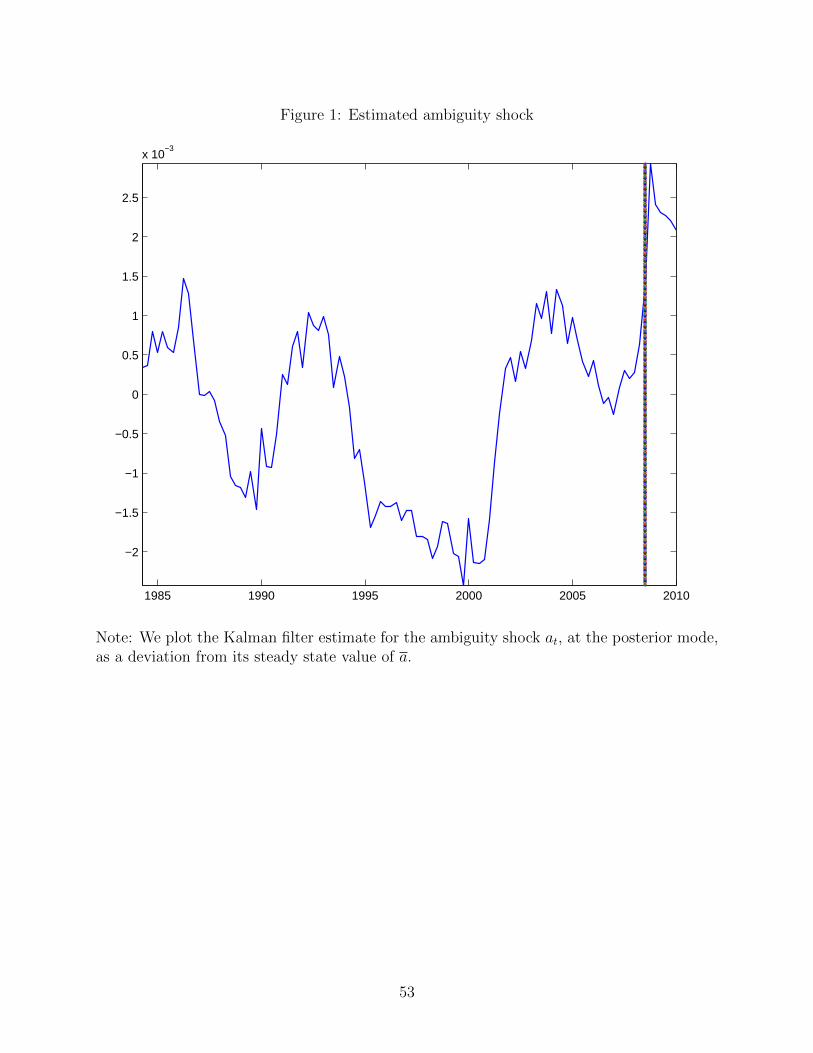
Figure 1: Estimated ambiguity shock

1985 1990 1995 2000 2005 2010

−2

−1.5

−1

−0.5

0

0.5

1

1.5

2

2.5

x 10−3

Note: We plot the Kalman filter estimate for the ambiguity shock at, at the posterior mode,as a deviation from its steady state value of a.

53

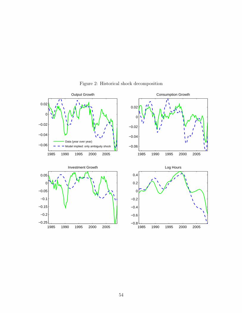
Figure 2: Historical shock decomposition

1985 1990 1995 2000 2005

−0.06

−0.04

−0.02

0

0.02

Output Growth

Data (year over year)

Model implied: only ambiguity shock

1985 1990 1995 2000 2005

−0.06

−0.04

−0.02

0

0.02

Consumption Growth

1985 1990 1995 2000 2005−0.25

−0.2

−0.15

−0.1

−0.05

0

0.05

Investment Growth

1985 1990 1995 2000 2005−0.8

−0.6

−0.4

−0.2

0

0.2

0.4

Log Hours

54

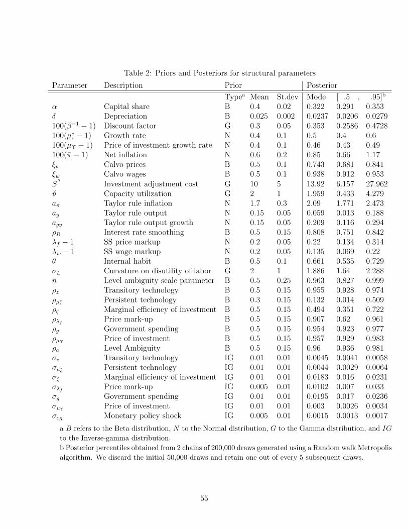
Table 2: Priors and Posteriors for structural parameters

Parameter Description Prior Posterior

Typea Mean St.dev Mode [ .5 , .95]b

α Capital share B 0.4 0.02 0.322 0.291 0.353δ Depreciation B 0.025 0.002 0.0237 0.0206 0.0279100(β−1 − 1) Discount factor G 0.3 0.05 0.353 0.2586 0.4728100(µ∗ε − 1) Growth rate N 0.4 0.1 0.5 0.4 0.6100(µΥ − 1) Price of investment growth rate N 0.4 0.1 0.46 0.43 0.49100(π − 1) Net inflation N 0.6 0.2 0.85 0.66 1.17ξp Calvo prices B 0.5 0.1 0.743 0.681 0.841ξw Calvo wages B 0.5 0.1 0.938 0.912 0.953S′′

Investment adjustment cost G 10 5 13.92 6.157 27.962ϑ Capacity utilization G 2 1 1.959 0.433 4.279aπ Taylor rule inflation N 1.7 0.3 2.09 1.771 2.473ay Taylor rule output N 0.15 0.05 0.059 0.013 0.188agy Taylor rule output growth N 0.15 0.05 0.209 0.116 0.294ρR Interest rate smoothing B 0.5 0.15 0.808 0.751 0.842λf − 1 SS price markup N 0.2 0.05 0.22 0.134 0.314λw − 1 SS wage markup N 0.2 0.05 0.135 0.069 0.22θ Internal habit B 0.5 0.1 0.661 0.535 0.729σL Curvature on disutility of labor G 2 1 1.886 1.64 2.288n Level ambiguity scale parameter B 0.5 0.25 0.963 0.827 0.999ρz Transitory technology B 0.5 0.15 0.955 0.928 0.974ρµ∗ε Persistent technology B 0.3 0.15 0.132 0.014 0.509ρζ Marginal efficiency of investment B 0.5 0.15 0.494 0.351 0.722ρλf Price mark-up B 0.5 0.15 0.907 0.62 0.961ρg Government spending B 0.5 0.15 0.954 0.923 0.977ρµΥ

Price of investment B 0.5 0.15 0.957 0.929 0.983ρa Level Ambiguity B 0.5 0.15 0.96 0.936 0.981σz Transitory technology IG 0.01 0.01 0.0045 0.0041 0.0058σµ∗ε Persistent technology IG 0.01 0.01 0.0044 0.0029 0.0064σζ Marginal efficiency of investment IG 0.01 0.01 0.0183 0.016 0.0231σλf Price mark-up IG 0.005 0.01 0.0102 0.007 0.033σg Government spending IG 0.01 0.01 0.0195 0.017 0.0236σµΥ

Price of investment IG 0.01 0.01 0.003 0.0026 0.0034σεR Monetary policy shock IG 0.005 0.01 0.0015 0.0013 0.0017

a B refers to the Beta distribution, N to the Normal distribution, G to the Gamma distribution, and IG

to the Inverse-gamma distribution.b Posterior percentiles obtained from 2 chains of 200,000 draws generated using a Random walk Metropolis

algorithm. We discard the initial 50,000 draws and retain one out of every 5 subsequent draws.

55

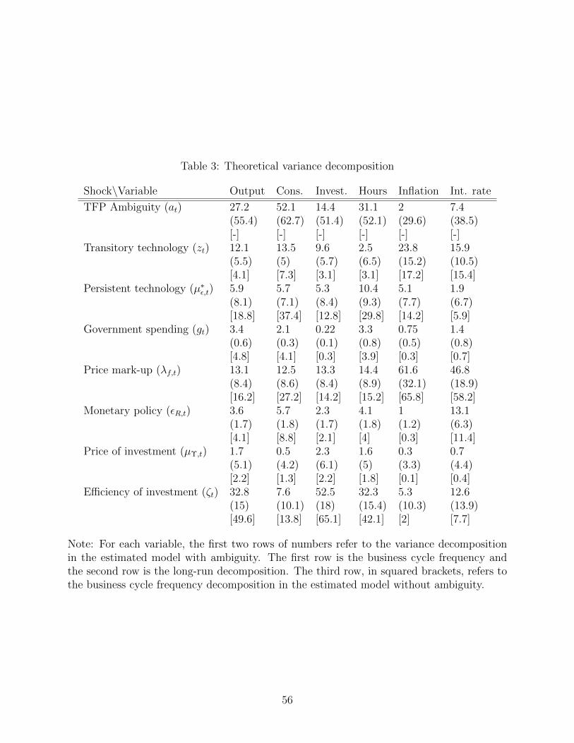
Table 3: Theoretical variance decomposition

Shock\Variable Output Cons. Invest. Hours Inflation Int. rate

TFP Ambiguity (at) 27.2 52.1 14.4 31.1 2 7.4(55.4) (62.7) (51.4) (52.1) (29.6) (38.5)[-] [-] [-] [-] [-] [-]

Transitory technology (zt) 12.1 13.5 9.6 2.5 23.8 15.9(5.5) (5) (5.7) (6.5) (15.2) (10.5)[4.1] [7.3] [3.1] [3.1] [17.2] [15.4]

Persistent technology (µ∗ε,t) 5.9 5.7 5.3 10.4 5.1 1.9(8.1) (7.1) (8.4) (9.3) (7.7) (6.7)[18.8] [37.4] [12.8] [29.8] [14.2] [5.9]

Government spending (gt) 3.4 2.1 0.22 3.3 0.75 1.4(0.6) (0.3) (0.1) (0.8) (0.5) (0.8)[4.8] [4.1] [0.3] [3.9] [0.3] [0.7]

Price mark-up (λf,t) 13.1 12.5 13.3 14.4 61.6 46.8(8.4) (8.6) (8.4) (8.9) (32.1) (18.9)[16.2] [27.2] [14.2] [15.2] [65.8] [58.2]

Monetary policy (εR,t) 3.6 5.7 2.3 4.1 1 13.1(1.7) (1.8) (1.7) (1.8) (1.2) (6.3)[4.1] [8.8] [2.1] [4] [0.3] [11.4]

Price of investment (µΥ,t) 1.7 0.5 2.3 1.6 0.3 0.7(5.1) (4.2) (6.1) (5) (3.3) (4.4)[2.2] [1.3] [2.2] [1.8] [0.1] [0.4]

Efficiency of investment (ζt) 32.8 7.6 52.5 32.3 5.3 12.6(15) (10.1) (18) (15.4) (10.3) (13.9)[49.6] [13.8] [65.1] [42.1] [2] [7.7]

Note: For each variable, the first two rows of numbers refer to the variance decompositionin the estimated model with ambiguity. The first row is the business cycle frequency andthe second row is the long-run decomposition. The third row, in squared brackets, refers tothe business cycle frequency decomposition in the estimated model without ambiguity.

56

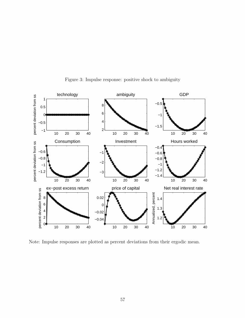
Figure 3: Impulse response: positive shock to ambiguity

10 20 30 40−1

−0.5

0

0.5

1technology

perc

ent d

evia

tion

from

ss

10 20 30 402

4

6

8

ambiguity

10 20 30 40

−1.5

−1

−0.5

GDP

10 20 30 40

−1.2

−1

−0.8

−0.6

Consumption

perc

ent d

evia

tion

from

ss

10 20 30 40

−3

−2

−1

Investment

10 20 30 40−1.4

−1.2

−1

−0.8

−0.6

−0.4

Hours worked

10 20 30 400

2

4

6

8

ex−post excess return

perc

ent d

evia

tion

from

ss

10 20 30 40

−0.04

−0.02

0

0.02

price of capital

10 20 30 40

1.2

1.3

1.4

Net real interest rate

Ann

ualiz

ed, p

erce

nt

Note: Impulse responses are plotted as percent deviations from their ergodic mean.

57