1

MINISTRY OF ENVIRONMENT

PROVINCE OF BRITISH COLUMBIA

Ambient Water Quality Guidelines For Sulphate

Technical Appendix

Update

April 2013

Prepared by:

Cindy Meays, Ph.D.

and

Rick Nordin, Ph.D.

Water Protection & Sustainability Branch

Environmental Sustainability and Strategic Policy Division

BC Ministry of Environment

2

Acknowledgements

We would like to thank Dr. Carl Schwarz for his statistical analysis and guidance on this

guideline. We would like to thank Graham Van Aggelen, Craig Buday, and Grant Schroeder at

the Pacific & Yukon Laboratory for Environmental Testing and Dr. Chris Kennedy from Simon

Fraser University for conducting toxicity tests to update this guideline. We would also like to

thank the Mining Association of BC and the Mining Association of Canada for providing their

toxicity data to update this guideline. Special thanks to Kevin Rieberger and George Butcher for

their technical and editorial contributions which substantially improved this guideline. We

would also like to thank Geneen Russo, Bruce Carmichael, Jody Fisher, James Jacklin, Craig

Stewart, Chris Stroich, John Deniseger, Deb Epps, Celine Davis, Kim Bellefontaine, Greg

Tamblyn, Carrie Morita, Julie Orban, Vic Jensen, Pat Shaw, Les McDonald, James Elphick,

Barry Zajdlik, John Chapman, Kevin Boon, Doug Spry, Susan Roe, Monica Nowierski, Kevin

Haines, Harvey McLeod, and Liam Mooney for their editorial contributions and review

comments.

3

Table of Contents

Summary..........................................................................................................................................6

PART A – Introduction.................................................................................................................8

PART B - General Review of Sulphate......................................................................................10

1.0 Physical and Chemical Properties............................................................................................10

1.1 Analytical Technique...................................................................................................12

2.0 Occurrence in the Environment...............................................................................................12

2.1 Natural Sources............................................................................................................12

2.2 Anthropogenic Sources................................................................................................12

2.3 Uses..............................................................................................................................13

2.4 Remediation.................................................................................................................14

2.5 Sulphate Concentrations in Receiving Waters.............................................................15

2.5.1 Freshwater.....................................................................................................15

2.5.2 Seawater........................................................................................................16

3.0 Sulphate Toxicity to Aquatic Organisms.................................................................................17

4.0 Water Hardness........................................................................................................................20

5.0 Indirect Effects of Sulphate.....................................................................................................21

5.1 Eutrophication Associated with Sulphate....................................................................21

5.2 Mercury Methylation Associated with Sulphate..........................................................22

PART C – Review of Sulphate Guidelines.................................................................................23

6.0 Current BC Sulphate Guideline...............................................................................................23

6.1 Criticisms of the Current BC Sulphate Guideline........................................................24

7.0 Sulphate Guidelines for Aquatic Life from other Jurisdictions...............................................25

8.0 Raw Drinking Water................................................................................................................26

8.1 Drinking Water Guidelines from the Literature...........................................................26

9.0 Effects of Sulphate on Livestock.............................................................................................27

PART D –Updated Sulphate Guidelines....................................................................................28

10.0 Recent Data Used to Update the Sulphate Water Quality Guidelines...................................28

10.1 Elphick et al. (2011) Published Data.........................................................................28

10.2 PESC and Kennedy Data...........................................................................................29

10.3 Toxicity Test Methods...............................................................................................30

11.0 Statistical Analysis.................................................................................................................32

11.1 Mortality Responses.......................................................................................34

11.2 Continuous Responses...................................................................................35

11.3 Model Ranking and Fitting............................................................................37

11.4 Model Averaging and Calculation of Benchmark Dose................................37

12.0 Results....................................................................................................................................41

13.0 Discussion and Application of a Sulphate Guideline............................................................42

14.0 Sulphate Water Quality Guidelines for the Protection of Aquatic Life.................................46

15.0 Literature Cited......................................................................................................................47

4

List of Tables

Table 1. Summary of ambient dissolved sulphate concentrations in BC freshwaters..................15

Table 2. A summary of protocols used by PESC, Kennedy and Elphick et al. (2011)................31

Table 3. Model averaged estimates (mg/L) for PESC sulphate toxicity data...............................39

Table 4. Model averaged estimates (mg/L) for Kennedy’s 21-d rainbow trout early life

stage sulphate toxicity data..............................................................................................40

Table 5. Model averaged estimates (mg/L) for Elphick et al. (2011) sulphate toxicity data

data...................................................................................................................................40

Table 6. Sulphate water quality guidelines (mg/L) based on water hardness (mg/L)

categories........................................................................................................................46

List of Figures

Figure 1. The sulfur cycle (taken from Fenchel et al. 2000). ........................................................11

Figure 2. Annual cycle of dissolved sulphate in the Bear River at Stewart BC

(1987-1995)....................................................................................................................16

Figure 3. Schematic of model types used to estimate sulphate toxicity at different

water hardness…………………………………………………………………………33

Figure 4. Schematic of probit regression models fitted for mortality responses of sulphate

using maximum likelihood methods………………………………………………….33

Figure 5. Schematic of isotonic regression models fitted for continuous responses

(e.g. weight, reproduction etc.) to sulphate using maximum likelihood methods……..34

Figure 6. Schematic of log-logistic models fitted for continuous responses (e.g. weight,

reproduction etc.) to sulphate using maximum likelihood methods…………………..34

Figure 7. Model averaged sulphate toxicity versus water hardness for 21-d rainbow

trout embryo to alevin life stage from 2011 Kennedy study…………………………44

Figure 8. All model averaged sulphate toxicity endpoints from Elphick et al. (2011),

PESC and Kennedy studies plotted against the water quality guideline……………..45

5

List of Appendices

APPENDIX A – Supporting information (water chemistry, control mortality) for toxicity

tests conducted by PESC

APPENDIX B – Report and data analysis for rainbow trout toxicity tests conducted by

Kennedy

APPENDIX C - Supporting information (water chemistry, control mortality) for toxicity

tests conducted by Elphick et al. (2011).

APPENDIX D - Statistical Analysis conducted by Dr. Carl Schwarz using Maximum

Likelihood Estimation.

APPENDIX E - Model Averaging Analysis conducted by Dr. Carl Schwarz

List of Abbreviations

AIC – Akaike Information Criterion

ARD – Acid rock drainage

BMD – Benchmark dose

CCME – Canadian Council of Ministers of the Environment

CETIS – Comprehensive Environmental Toxicity Information System

EC – effect concentration

IC – inhibition concentration

LC – lethal concentration (LC50, concentration of toxicant that kills 50% of the organisms

tested).

LOEC – lowest observed effects concentration

MLE – maximum likelihood estimation

NOEC – no observed effects concentration

PESC – Pacific Environmental Science Centre

6

Summary

Sulphate is a potentially harmful contaminant in freshwater environments. In 2000, Singleton

developed a maximum water quality guideline of 100 mg/L for British Columbia (BC) to protect

freshwater aquatic life. At that time, there were insufficient chronic toxicity data to develop a

30-day average guideline. Over the last 10 years, research has provided new information on the

aquatic toxicology of sulphate prompting a review and update of the 2000 water quality

guideline. This review includes the recent scientific literature and additional research

commissioned by the BC Ministry of Environment focussing on the chronic toxicity of sulphate.

The majority of sulphate toxicity studies reported in the literature have been acute exposures

conducted with aquatic invertebrates. Since very few chronic toxicity studies on sulphate have

been reported, the BC MOE contracted the Pacific Environmental Science Center (PESC) and

Dr. Chris Kennedy (at Simon Fraser University) to conduct and coordinate a series of sulphate

toxicity tests over a range of water hardnesses, using various freshwater species of aquatic

organisms. In 2011, Elphick et al. also published results of experiments testing the relationships

between sulphate toxicity and water hardness for several aquatic species. Data from all 3 studies

were used to update the sulphate water quality guideline.

Statistical analysis of the data from the recent studies found that while the dose-response curves

of many organisms were influenced by water hardness, a consistent relationship among the

species could not be established. The most sensitive species tested was rainbow trout (the 21-d

embryo to alevin life stage) which demonstrated some amelioration of sulphate toxicity with

increasing water hardness from 6 mg/L up to 250 mg/L. As a result sulphate water quality

guidelines for the protection of aquatic life were developed for different categories of water

hardness based on the rainbow trout LC20 data with the minimal uncertainty factor of 2 applied.

7

The approved 30-day average (minimum of 5 evenly-spaced samples collected in 30 days) water

quality guidelines to protect aquatic life in BC for sulphate are:

Water hardness* (mg/L) Sulphate guideline (mg/L) Very Soft (0-30) 128 Soft to moderately soft (31-75) 218 Moderately soft/hard to hard (76-180) 309 Very hard (181-250) 429 >250 Need to determine based on site water**

*Water hardness categories adapted from the CCME.

** Toxicity tests on the early stage rainbow trout were only conducted up to a water hardness of 250 mg/L. Natural

background concentrations of water hardness in BC are generally much lower than 250 mg/L. It is recommended

that additional toxicity testing on several species is required if natural background water hardness is greater than 250

mg/L. Organisms exposed to higher concentrations of water hardness in combination with sulphate may experience

osmotic stress.

The original data from the PESC 1996 studies was unavailable, therefore we were unable to

classify the studies or use them to develop a short-term maximum guideline. There is no short-

term maximum guideline to protect aquatic life proposed at this time.

The approved water quality guidelines to protect human health and livestock use are:

Water Use Sulphate guideline (mg/L) Drinking water 500 Agriculture (livestock use)* 1,000

*Note: CCME is in the process of updating the livestock use guideline for sulphate.

This report consists of 4 parts:

PART A – Introduction

PART B − General Review of Sulphate

PART C – Review of Current Sulphate Guidelines

PART D – Updated Sulphate Guidelines

8

PART A – Introduction

Sulphate concentrations in water are the result of natural weathering of minerals, atmospheric

deposition, and anthropogenic discharges. Sulphates are discharged into the aquatic environment

in wastes from industrial sources such as mining and smelting operations, kraft pulp and paper

mills, textile mills and tanneries. In British Columbia (BC), the toxicity to aquatic life from

dissolved sulphate discharged in the environment is of particular interest. In 2000, Singleton

proposed a maximum water quality guideline of 100 mg/L for sulphate in freshwater to protect

aquatic life. Since that time, new research and information on sulphate toxicity has been

reported in the scientific literature prompting the review of the current guideline. This document

focuses primarily on the protection of aquatic life from the long-term (chronic) effects of

sulphate toxicity, but also considers the effects of sulphate on other water uses including

drinking water and livestock watering.

The BC Ministry of Environment (MOE) develops province-wide ambient water quality

guidelines for substances or physical attributes that are important for managing both fresh and

marine surface waters of BC. This work has the following goals:

to provide protection of the most sensitive aquatic life form and most sensitive life stage

indefinitely;

to provide a basis for the evaluation of data on water, sediment, and biota for water

quality and environmental impact assessments;

to provide a basis for the establishment of site-specific ambient water quality objectives;

to identify areas with degraded conditions that need remediation;

to provide a basis for establishing wastewater discharge limits; and

to report to the public on the state of water quality and promote water stewardship.

BC water quality guidelines are science-based and intended for generic provincial application.

They do not account for site-specific conditions or socio-economic factors. All components of

the aquatic ecosystem (e.g. algae, macrophytes, invertebrates, amphibians, and fish) are

9

considered if the data are available. Where data are available but limited, interim guidelines may

be developed.

The approach to develop guidelines for aquatic life reflects the policy that all forms of aquatic

life and all aquatic stages of their life cycle are to be protected during indefinite exposure. For

some substances both a short-term maximum and a 30-day average (long-term) guideline are

recommended as provincial water quality guidelines, provided sufficient toxicological data are

available. Both conditions should be met to protect aquatic life.

The goal of freshwater aquatic life guidelines is the protection and maintenance of all forms of

aquatic life and all life stages in the freshwater environment. Therefore, it is essential that, at a

minimum, data for fish, invertebrates, and plants be included in the guidelines derivation

process. Data from amphibians are also highly desirable. Guidelines or interim guidelines may

also include studies involving species not required in the minimum data set (e.g. protozoa,

bacteria) when reasonable justification exists.

It should be noted that there are several sources of uncertainty when it comes to developing

water quality guidelines and therefore it is necessary to apply uncertainty factors. Sources of

uncertainty include:

laboratory to field differences;

single to multiple contaminants (additive, synergistic, antagonistic effects);

toxicity of metabolites;

intra and inter-species differences (limited species to conduct tests on, which may not

include the most sensitive species);

indirect effects (e.g. foodweb dynamics);

whole life-cycle vs. partial life-cycle (many toxicity studies are only conducted on partial

life-cycles and it can be difficult to determine the most sensitive life stage);

delayed effects;

impacts of climate change (species may be more vulnerable with additional stressors);

and

10

other stressors including cumulative effects.

The appropriate uncertainty factor to be applied is decided on a case-by-case basis and is based

on data quality and quantity, toxicity of the contaminant, severity of toxic effects, and

bioaccumulation potential (BC MoE 2012). Scientific judgement is used to maintain some

flexibility in the derivation process.

Presently, water quality guidelines do not have any direct legal standing. They are intended as a

tool to provide policy direction to those making decisions affecting water quality provided that

they do not allow legislated effluent standards to be exceeded. Water quality guidelines can be

used to establish the allowable limits in waste discharges. These limits are set out in waste

management permits, approvals, plans, or operating certificates which do have legal standing.

PART B – A General Review of Sulphate

1.0 Physical and Chemical Properties

In inorganic chemistry, sulphate (also sulfate: The International Union of Pure and Applied

Chemistry-recommended spelling) is a salt of sulphuric acid. The sulphate ion is a polyatomic

anion with the empirical formula SO42–

and a molecular mass of 96.06 daltons (96.06 g/mol). It

consists of a central sulphur atom surrounded by 4 equivalent oxygen atoms in a tetrahedral

arrangement. The sulphur atom is in the +6 oxidation state while the 4 oxygen atoms are each in

the –2 state, therefore the sulphate ion carries a –2 charge. Sulphur is an essential element for all

forms of life. In plants and animals the amino acids cysteine and methionine contain sulphur, as

do all polypeptides, proteins, and enzymes that contain these amino acids.

Sulphur moves through a number of forms (generally described as the sulphur cycle) depending

on environmental conditions. Sulphur is such a ubiquitous element and so involved in biological

processes that Monheimer (1975), who reported measures of sulphate uptake by microplankton

in Lake St. Clair, proposed the use of sulphate uptake as a general measure of microbial

production (phytoplankton and bacteria). A review of the sulphur cycle is described in Kellogg

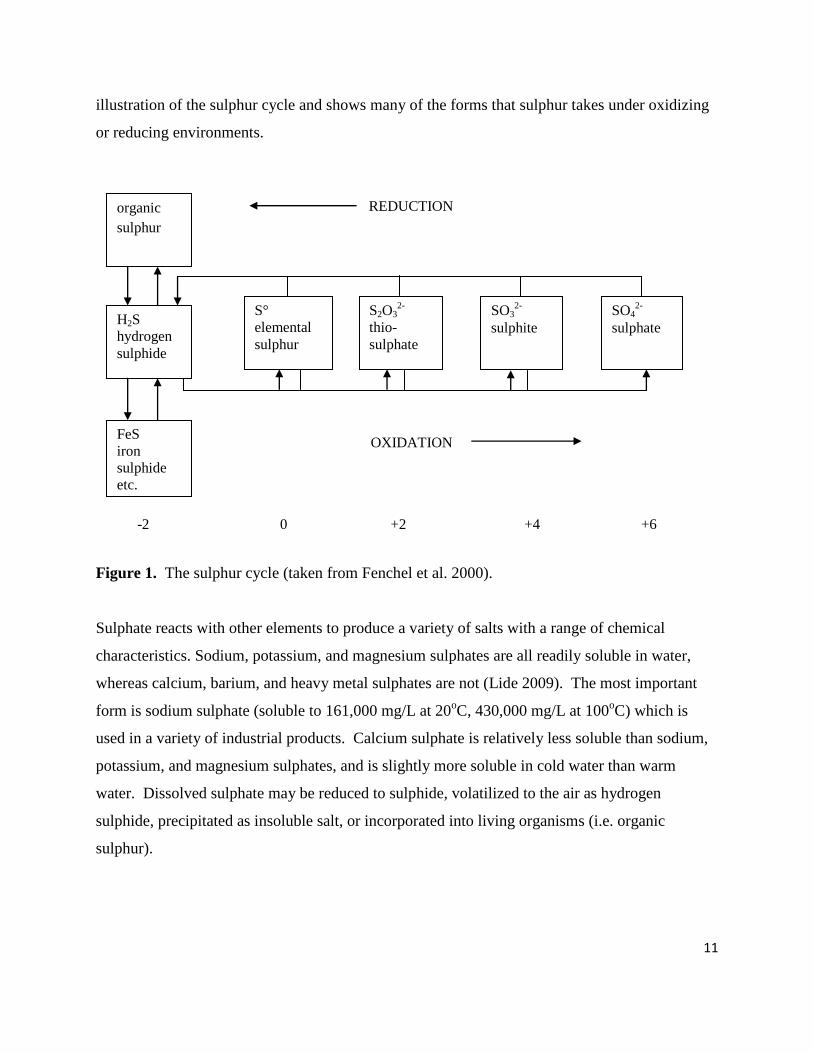
et al. (1972) and the bacterial interactions in Jørgensen (1982). Figure 1 is a generalized

11

illustration of the sulphur cycle and shows many of the forms that sulphur takes under oxidizing

or reducing environments.

Figure 1. The sulphur cycle (taken from Fenchel et al. 2000).

Sulphate reacts with other elements to produce a variety of salts with a range of chemical

characteristics. Sodium, potassium, and magnesium sulphates are all readily soluble in water,

whereas calcium, barium, and heavy metal sulphates are not (Lide 2009). The most important

form is sodium sulphate (soluble to 161,000 mg/L at 20oC, 430,000 mg/L at 100

oC) which is

used in a variety of industrial products. Calcium sulphate is relatively less soluble than sodium,

potassium, and magnesium sulphates, and is slightly more soluble in cold water than warm

water. Dissolved sulphate may be reduced to sulphide, volatilized to the air as hydrogen

sulphide, precipitated as insoluble salt, or incorporated into living organisms (i.e. organic

sulphur).

organic

sulphur

FeS

iron

sulphide

etc.

H2S

hydrogen

sulphide

S°

elemental

sulphur

S2O32-

thio-

sulphate

SO32-

sulphite

SO42-

sulphate

REDUCTION

OXIDATION

-2 +4 +6 +2 0

12

1.1 Analytical Techniques

While other methods are available, sulphate in aqueous solutions is often determined by ion

chromatography using a conductivity detector; the detection limit for this method is about 0.03

mg/L (APHA 1985).

2.0 Occurrence in the Environment

2.1 Natural Sources

Sulphur occurs naturally in its reduced form in both igneous and sedimentary rocks as metallic

sulphides (e.g. FeS). Sulphate occurs in numerous minerals, including barite (BaSO4), epsomite

(MgSO4∙7H2O), gypsum (CaSO4∙2H2O), and mirabilite (Na2SO4·10H2O). In some areas of BC,

sulphate and hydrogen sulphide levels can be naturally elevated in groundwater. When sulphide

minerals undergo weathering in the presence of water, the sulphide is oxidized to yield soluble

sulphate ions. Hexavalent sulphur combines with oxygen to form the divalent sulphate ion

(SO42–

). The reversible reaction between sulphide and sulphate in the natural environment is

governed by a number of biological, chemical, and physical factors. Natural sources of

dissolved sulphur in water include mineral weathering, input from volcanoes, decomposition,

combustion of organic matter, and sea salt.

Lewicka-Szczebak et al. (2008) discuss the application of sulphur stable isotope (34

S) data to

distinguish sources of sulphur. Stable isotopes provide a useful tool to discriminate between

various potential sources of sulphate ions in freshwater environments from either natural (e.g.

dissolution of sulphate minerals, oxidation of pyrite, oxidation of organic sulphur by

microorganisms) or anthropogenic origins (e.g. acid rain, industry, sewage and agrochemical

contamination).

2.2 Anthropogenic Sources

Sulphates are discharged into aquatic environments through wastes from industries that produce

and/or use sulphates and sulphuric acid, such as mining and smelting operations, kraft pulp and

paper mills, textile mills, tanneries, agricultural run-off and sewage. High sulphate

concentrations are of particular concern to the mining industry (Davies 2007). Mining

13

development in BC is rapidly expanding. BC is Canada’s largest exporter of coal, and largest

producer of copper and molybdenum (MEMPR 2009). A major concern in BC and the US is the

effect on the aquatic environment of coal mining activities – especially large-scale mountain top

mining with valley fills (Palmer et al. 2010) which increases the total dissolved solids (TDS),

conductivity, and sulphate of local surface waters. Base and precious metal mines (both

abandoned and active) may be significant sources of sulphate through non-biological and

biological oxidation of sulphide minerals (pyrites). Acid rock drainage (ARD) and acidophilic

bacteria can exacerbate sulphate release to the aquatic environment. Treatment of ARD to reduce

the high acidity and toxic metal concentrations (e.g. lime addition) can lower sulphate levels (via

reaction with calcium to produce gypsum, CaSO4); however, dissolved sulphate levels can

remain very high in the resulting effluent. Sulphates can also be released as a result of blasting

(increasing of particle surface areas) and the deposition of waste rock in dumps at metal mines.

Sulphate has been used as a potential indicator of ARD.

In the eastern US, acidification of receiving waters exposed to mine drainage is an issue (Herlihy

et al. 1990). In BC, coal mining occurs predominantly in carbonate lithologies, where surface

waters have naturally higher hardness and pH (McDonald personal communication 2011).

Sulphate release from waste rock at the coal mines is due to oxidation of pyrites associated with

the coal. Carbonates from the host rock immediately neutralize the resulting acid. Sulphate

produced from the coal mine waste dumps is accompanied by the dissolution of dolomite which

causes similar magnitude increases in Ca2+

, Mg2+

and HCO3–. Mining is the primary source of

sulphate generation in BC, with concentrations in water draining mining operations ranging from

10 to 2,000 (or more) mg/L (BC MOE Environmental Management System database).

The burning of fossil fuels, particularly high-sulphur coal and diesel, is a major source of sulphur

to the atmosphere.

2.3 Uses

The world-wide production of sodium sulphate was about 4.6 million tonnes in 1999, about 50%

of which was as a by-product of chemical industries and the remainder produced from mining

deposits in ancient lakes (OECD 2006). The largest exporter of sodium sulphate is China

14

(Suresh and Yokose 2006). Two major users of sodium sulphate are the detergent and glass

industries. The detergent industry uses about 1 Mt annually primarily as filler in powdered home

laundry detergents. This use is waning, especially in North America, as domestic consumers are

switching to compact or liquid detergents that do not include sodium sulphate. The average

concentration of sodium sulphate in commercial detergents from European manufacturers is 21%

with the range from 0 to 57%. The glass industry provides another significant industrial

application for sodium sulphate. Sodium sulphate is used as a fining agent to help remove small

air bubbles from molten glass and prevents scum formation of the melt during refining. The

glass industry in Europe has consumed approximately 110,000 t annually from 1970 to 2006

(Suresh and Yokose 2006).

Historically, a major use of sodium sulphate in the US and Canada was in the kraft process for

the manufacture of wood pulp. Organics present in the "black liquor" from this process were

burnt to produce heat needed to drive the reduction of sodium sulphate to sodium sulphide.

However, this process is gradually being replaced by newer techniques. The use of sodium

sulphate in the US and Canadian pulp industry declined from 1.4 Mt/year in 1970 to

approximately 0.15 Mt/year in 2006 (Suresh and Yokose 2006).

Other industrial uses of sodium sulphate include dye making, electrochemical metal treatment,

animal feeds, pharmaceuticals, textiles, semiconductors, and fertilizers (OECD 2006).

2.4 Remediation

A variety of efforts have been made to reduce the impacts of sulphate to the environment from

mining. Lindsay et al. (2009) describe an experiment to increase microbial sulphate reduction in

mine tailing deposits by adding organic carbon (brewing waste). The organic carbon additions

resulted in decreases in dissolved SO42–

and S2O3 and increased H2S and a general decrease in

mass transport of sulphide oxidation products. Jegadeesan et al. (2005) describe a 2-stage

process for removal of selenium and sulphate from water using barium chloride in the first stage

followed by a selenium remediation agent (bimetallic NiFe particles, alumina and activated

carbon) in the second. The International Network for Acid Prevention (2003) provides a review

15

of treatment of sulphate in mine effluents. Policy guidance for managing impacts from hardrock

mines, specifically those in sulphide mineral geology, is provided by Kempton et al. (2010).

2.5 Sulphate Concentrations in Receiving Waters

2.5.1 Freshwater

Natural background sulphate concentrations in Canadian lakes typically range from 3 to 30 mg/L

(Katz 1977). In a survey of river waters in the prairie provinces of Canada, sulphate

concentrations ranged from 1 to 3,040 mg/L; most concentrations were below 580 mg/L

(Environment Canada 1984).

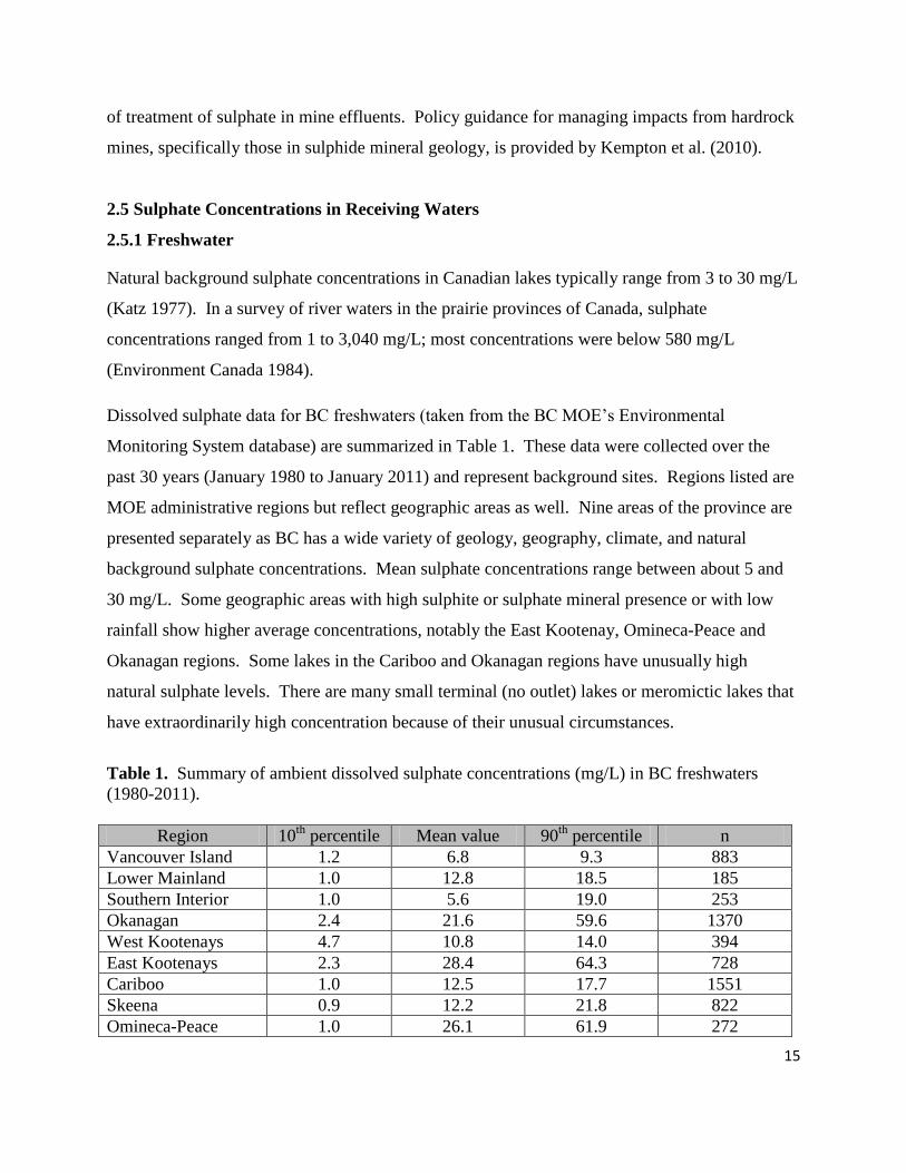
Dissolved sulphate data for BC freshwaters (taken from the BC MOE’s Environmental

Monitoring System database) are summarized in Table 1. These data were collected over the

past 30 years (January 1980 to January 2011) and represent background sites. Regions listed are

MOE administrative regions but reflect geographic areas as well. Nine areas of the province are

presented separately as BC has a wide variety of geology, geography, climate, and natural

background sulphate concentrations. Mean sulphate concentrations range between about 5 and

30 mg/L. Some geographic areas with high sulphite or sulphate mineral presence or with low

rainfall show higher average concentrations, notably the East Kootenay, Omineca-Peace and

Okanagan regions. Some lakes in the Cariboo and Okanagan regions have unusually high

natural sulphate levels. There are many small terminal (no outlet) lakes or meromictic lakes that

have extraordinarily high concentration because of their unusual circumstances.

Table 1. Summary of ambient dissolved sulphate concentrations (mg/L) in BC freshwaters

(1980-2011).

Region 10th

percentile Mean value 90th

percentile n

Vancouver Island 1.2 6.8 9.3 883

Lower Mainland 1.0 12.8 18.5 185

Southern Interior 1.0 5.6 19.0 253

Okanagan 2.4 21.6 59.6 1370

West Kootenays 4.7 10.8 14.0 394

East Kootenays 2.3 28.4 64.3 728

Cariboo 1.0 12.5 17.7 1551

Skeena 0.9 12.2 21.8 822

Omineca-Peace 1.0 26.1 61.9 272

16

Seasonal fluctuations in dissolved sulphate concentrations are apparent in most rivers, with low

concentrations during freshet and elevated concentrations during the low flow periods as shown

for the Bear River at Stewart, BC (Figure 2). Changes in sulphate concentrations can also be

event-driven. Rain-dominated coastal streams can be quite different from snow-dominated

northern or interior systems.

Figure 2. Annual cycle of dissolved sulphate in the Bear River at Stewart, BC (1987-1995).

2.5.2 Seawater

Seawater contains about 2,700 mg/L sulphate (Hitchcock 1975) and it has been estimated that

about 1.7 Mt of sulphate are added annually to the Canadian atmosphere from sea spray (Katz

1977). The largest biological source of sulphur to the atmosphere is from decay of planktonic

algae and bacteria and release in the form of dimethyl sulfide gas.

17

3.0 Sulphate Toxicity to Aquatic Organisms

Sulphate toxicity studies have focussed on 3 groups of organisms: algae and aquatic plants,

aquatic invertebrates, and fish. Until recently, the majority of studies have focussed on the acute

toxicity of sulphate to aquatic invertebrates. Mount et al. (1997) derived statistical models of

toxicity of major ions to Ceriodaphnia dubia (water flea), Daphnia magna (water flea) and

Pimephales promelas (fathead minnow). Of the relative toxicity reported, sulphate was the least

toxic (K+

> HCO3–

= Mg2+

> Cl– > SO4

2–). Borgmann (1996) examined the ion requirements of

Hyalella azteca (scud) and concluded that sulphate is not required for survival, growth or

reproduction.

Lasier and Hardin (2010) did an evaluation of chloride, sulphate and bicarbonate chronic toxicity

to C. dubia. Sulphate was noted as being less toxic than chloride or bicarbonate. Water hardness

significantly affected chloride and sulphate toxicity, but had little effect on bicarbonate toxicity.

Mean inhibitory concentrations (IC25 and IC50) and coefficients of variation (CV) were given

for different concentrations of hardness and alkalinity. At low hardness and alkalinity (44 mg/L

hardness, 45 mg/L alkalinity) they reported a 7-day IC25 of 625 mg/L (CV=14) and an IC50 of

766 mg/L (CV=13), at their intermediate hardness/alkalinity (93/66) the IC25 and IC50 were

1,060 (CV=4) and 1,252 mg/L (CV=5), respectively. At their low hardness and high alkalinity

(44/101) the IC25 and IC50 were 496 (CV=8) and 715 mg/L (CV=6) sulphate, respectively.

Soucek and Kennedy (2005) tested the effects of hardness, chloride, and acclimation on the acute

toxicity of sulphate to 4 species (C. dubia, Chironomus tentans (midge), H. azteca and

Sphaericum simile (grooved fingernail clam)). 48-hour LC50s for C. dubia and C. tentans and

96-hour LC50s for H. azteca and S. simile, expressed as mg/L SO42–

, in moderately hard

reconstituted water (MHRW) were as follows: 2,050 (1,869-2,270) mg/L for C. dubia; 14,134

(14,123-14,146) mg/L for C. tentans; 512 (431-607) mg/L for H. azteca; and 2,078 (1,901-2,319)

mg/L for S. simile. At a constant sulphate concentration (2,800 mg/L) and hardness (106 mg/L),

survival of H. azteca was positively correlated with chloride concentration. Hardness was also

found to ameliorate sodium sulphate toxicity to C. dubia and H. azteca, with LC50s for C. dubia

increasing from 2,050 (1,869-2,270) mg/L sulphate at hardness 90 mg/L to 3,516 (3,338-3,716)

18

mg/L sulphate at hardness 484 mg/L. Using a reformulated MHRW with a similar hardness but

higher chloride concentration and different calcium to magnesium ratio than that in standard

MHRW, the mean 96-hour LC50 for H. azteca increased to 2,855 (2,835-2,876) mg/L, and the

48-hour LC50 for C. dubia increased to 2,526 (2,436-2,607) mg/L. Acclimation of C. dubia to

500 and 1,000 mg/L SO42–

for several generations did not significantly increase the mean LC50

values compared with those cultured in standard MHRW.

Soucek (2007a) used an experimental approach to investigate the effect of sodium sulphate on C.

dubia toxicity using non-lethal indicators (fecundity or feeding rate) in experiments running 7

days and 5 generations. He noted decreased energy and fecundity over several generations.

Effects on fecundity were noted at concentrations of 899 mg/L SO42–

(lowest observed adverse

effect concentration (LOAEC) in moderately hard reconstituted water) which were less than half

the concentrations for survival (7-day LC50 of 2,049 mg/L SO42–

).

Soucek (2007b) quantified the influence of both chloride and water hardness on the acute

toxicity of sulphate to H. azteca and C. dubia. At 25 mg/L chloride, H. azteca sulphate toxicity

decreased with increasing water hardness up to 500 mg/L hardness, however the mean LC50

value decreased at 600 mg/L hardness as compared to the value at 500 mg/L. Increasing

chloride concentrations from 5 to 25 mg/L resulted in increased sulphate LC50s for H. azteca but

not C. dubia. However, a significantly negative trend in sulphate LC50s for both H. azteca and

C. dubia was observed over the range of chloride from 25 to 500 mg/L.

Soucek (2007c) demonstrated that sodium sulphate had no effect on basal metabolic rates of the

clam Corbicula fluminea (Asian clam), but significantly reduced feeding rates, post-feeding

metabolic rates, and growth rates in chronic (4-week, 1,500 mg/L SO42–

) exposures. Soucek

(2007c) suggested that in the field, these results could cause changes in whole stream respiration

rates and organic matter dynamics, including altering uptake rates of other food-associated

contaminants such as selenium in filter-feeding bivalves.

19

Elphick et al. (2011) reported long-term toxicity results for a number of invertebrate, fish, moss

and algae species for sulphate at various levels of water hardness. From their results, C. dubia

reproduction in soft (40 mg/L CaCO3) and very hard (320 mg/L CaCO3) water were the most

sensitive endpoints.

Sulphate is a large, bulky ion which is thought to be difficult for many insects to osmoregulate

(Conley et al. 2010). Some insect taxa such as Aedes (mosquito) are able to rapidly clear

sulphate from the haemolymph using an active transport mechanism allowing the aquatic life

stages to survive in water high in sulphates and other ions. Insect taxa which do not have this

active transport mechanism (e.g. Calliphora spp. (blow flies) and Rhodnius spp. (kissing bug))

are far less tolerant of high sulphate concentrations (Maddrell and Phillips 1975). In

ecotoxicological studies carried out in an experimental stream system, Goetsch and Palmer

(1997) found that Na2SO4 was considerably more toxic than NaCl to mayflies (Tricorythus sp.)

with 96-hour LC50s of 660 mg/L vs. 2,200-4,500 mg/L, respectively. They suggested that it is

necessary to investigate the physiology of these organisms to determine if mortality is caused by

osmoregulatory functioning through elevated TDS concentrations or chemical species (Na+,

SO42–

, or Cl–) disrupting essential enzymatic processes. Conley and Buchwalter (personal

communication 2011) conducted a pilot study investigating the toxicity of SO42–

on newly

hatched Centroptilum triangulifer (mayfly); the 10-day LC50 was 327 (200-534) mg/L, however

the exposure concentrations were not verified analytically. The results are considered

preliminary and further studies are needed.

Fewer sulphate toxicity data exist for fish. The early data of Trama (1954) using Lepomis

macrochirus (bluegill sunfish) gave a 96-hour LC50 concentration of 13,500 mg/L. Patrick et al.

(1968) also tested L. macrochirus and arrived at the same 96-hour LC50. Mount et al. (1997)

reported a 96-hour LC50 of 7,960 (6,800–10,000) mg/L for P. promelas. Elphick et al. (2011)

reported a 31-day EC10 and 10-day EC10 of 356 (256-433) and 941 (803-1,062) for O. mykiss

(rainbow trout) and Oncorhynchus kisutch (coho salmon) in soft (15 mg/L CaCO3) water,

respectively. They also reported a range of 7-day EC10/IC10 survival and growth data for P.

promelas depending on water hardness.

20

Even fewer sulphate toxicity studies exist for micro-organisms. Of the few studies found, Tokuz

and Eckenfelder (1979), Tokuz (1986), and Gilli and Comune (1980) looked at bacteria,

protozoa, and ciliates in activated sludge and found no apparent toxicity to at least 8,000 mg/L.

4.0 Water Hardness

Hard water can reduce the toxicity of some substances, particularly dissolved metals, to aquatic

organisms (see Section 3). Elphick et al. (2011) proposed sulphate water quality guidelines

based on water hardness. However, it is important to note that they also showed increased

sulphate toxicity in certain tests at water hardness levels above 160 mg/L CaCO3; they suggested

this could be the result of an osmotic challenge for some species. Elphick (personal

communication 2011) suggested that the effect at higher water hardness on C. dubia may not be

from sulphate, but instead might be from the ionic strength from the total dissolved solids (TDS).

Water hardness is a generic measure that does not reflect the specific composition and

concentration of different ions present in water. This is a concern for setting water quality

guidelines (Goodfellow et al. 2000) due to the potential differences in toxicity and toxicity

modifying effect among the different ions that contribute to hardness (primarily calcium and

magnesium), and different responses to contaminants in waters of similar hardness can be

expected depending on the specific ionic composition (Perschbacher and Wurts 1999; Welsh et

al. 2000a). Furthermore, the Ca2+

and Mg2+

concentrations in the recommended American

Society for Testing and Materials (ASTM) water (laboratory water) are different from those in

most natural surface waters. Welsh et al. (2000b) state that using the current US EPA water

effect ratio method can lead to water quality criteria that are under-protective of aquatic biota

because the method does not account for the differences in calcium and magnesium

concentrations (Ca:Mg ratios) found in natural waters. Davies and Hall (2007) also found that

the ratio of Ca:Mg can change toxicity of NaSO4 to H. azteca and D. magna.

The toxicity of MgSO4 has recently been assessed in Australia by van Dam et al. (2010). They

found that Mg2+

was much more toxic than sulphate to the species tested and that Mg2+

was

much more toxic than previously reported in the literature. They conclude that although Mg2+

21

and Ca2+

have historically been studied for their ameliorative properties on metal toxicity, Mg2+

can be toxic at very low concentrations to species that inhabit low ionic strength surface waters

in unusual cases where Ca2+

is substantially lower than Mg2+

.

Ketola et al. (1988) found that high concentrations of Ca2+

(> 520 mg/L) resulted in a marked

reduction in eye-up of Atlantic salmon (Salmo salar) eggs and significantly reduced survival of

Atlantic salmon, brook trout (Salvenlinus fontinalis), and rainbow trout. Ketola et al. (1988)

found that Atlantic salmon and trout eggs hardened (the swelling process of newly-shed eggs

caused by the absorption of water) in water with high Ca2+

concentrations had less turgor and

lower survival than those hardened within the first few hours in water with less Ca2+

. Stekoll et

al. (2009) conducted a study investigating the effects of major ions on the early developmental

stages of hatchery reared salmonids. They found the most sensitive life stage was fertilization

and that Ca2+

was a major contributor to decreases in fertilization success, although the

mechanism is not yet fully understood.

More research into the toxicity of Ca2+

and Mg2+

is needed since these are the major cations

released in alkaline mine runoff from coal mines with carbonate parent materials in BC

(McDonald personal communication 2011), and throughout much of the Central Appalachians

(Bernhardt and Palmer 2011).

5.0 Indirect Effects of Sulphate

Recent research suggests that elevated sulphate concentrations may have indirect effects on

aquatic ecosystems in terms of increasing phosphorus (P) availability and susceptibility to

eutrophication, and mercury mobilization. Further research in these areas is needed for better

understanding of these processes.

5.1 Eutrophication Associated with Sulphate

Increasing sulphate concentrations have the potential to lead to rising P mobilization rates in

riverine sediments (Zak et al. 2006), lake sediments (Curtis 1989), wetlands (Lamers et al. 1998;

Lamers et al. 2002; Smolders et al. 2003; Smolders et al. 2006; Van der Welle et al. 2007;

Smolders et al. 2010), marine sediments (Jørgensen 1982), and groundwater (Geurts et al. 2009).

22

Sulphate reduction can be a factor in increasing alkalinity of lakes (Schindler 1988). Curtis

(1989) found that the increased alkalinity from the reduction of sodium sulphate to sodium

sulphide increased P release in experimental enclosures placed in a small Precambrian Shield

lake.

Bacteria of the sulphur cycle are very important in P mobilization. Brouwer et al. (1999)

suggested that increased sulphate loading in sediments assists with P release by stimulating

mineralization by way of bacterial sulphate reduction. Sulphate additions at environmentally

relevant levels (192 and 384 mg/L) resulted in increased phosphate and alkalinity concentrations

in pore water. Sulphate reduction can also affect nutrient kinetics indirectly. Sulphide, produced

by bacterial sulphate reduction, interferes with iron-phosphate binding in soils and sediments due

to the formation of iron sulphides, which influences how phosphate is released in both marine

and freshwater sediments (Jørgensen 1982). The amount of phosphate released is dependent on

the availability of sulphate. Increasing sulphate results in increasing P mobilization; this can

potentially contribute to eutrophication in surface waters. Bernhardt and Palmer (2011) state that

sulphide is directly phototoxic to many aquatic plants.

5.2 Mercury Methylation Associated with Sulphate

Han et al. (2007) stated that one of the key factors that affect the rates of mercury methylation in

sediments is sulphate concentration and the rate of microbial sulphate reduction. Higher sulphate

concentrations result in higher rates of mercury methylation. Studies conducted with an

experimental wetland (Jeremiason et al. 2006) and a mesocosm (Harmon et al. 2004) also

reported that sulphate additions increase methyl mercury production. Methyl mercury is a bio-

available form of mercury which can biomagnify in the food web and can cause severe health

problems in humans (Kainz et al. 2008).

23

PART C – Review of Sulphate Guidelines

6.0 Previous BC Sulphate Guideline

The previous BC sulphate guideline for the protection of freshwater aquatic life was a maximum

of 100 mg/L (Singleton 2000). This guideline was based primarily on 4 pieces of evidence

demonstrating the toxic effects of sulphate on freshwater organisms. These were as follows:

i. Hughes (1973) reported 1-, 2-, 3-, and 4-day LC50's of 2,000, 1,000, 500, and 250 mg/L

for SO42–

, and LC0's (no effect) of 500, 100, 100, and 100 mg/L, respectively, for

Morone saxatilus (striped bass) larvae.

ii. Data from toxicity tests performed by the Pacific Environmental Science Centre (PESC)

for BC MOE in 1996 showed that the amphipod, H. azteca, was sensitive to sulphate in

soft water (25 mg/L as CaCO3), but not in medium (100 mg/L as CaCO3) to hard water

(250 mg/L as CaCO3). PESC reported 96-hour LC50s for H. azteca in soft, medium and

hard water of 205, 3,711 and 6,787 mg/L SO42–

, respectively. A water quality guideline

of 100 mg/L provided protection with a 2:1 uncertainty factor in soft water, and much

greater protection in harder water.

iii. Frahm (1975) reported that a concentration of 100 mg/L SO42–

was toxic to the aquatic

moss, Fontinalis antipyretica, a species widely distributed throughout BC. Toxicity of

SO42–

to 4 other species of aquatic moss ranged from 100 to >250 mg/L.

iv. Singleton (2000) stated that there is some evidence that elevated sulphate levels (average

of 71 mg/L sulphate; range of 27.7 to 189 mg/L) can stimulate large sulphur bacteria

growths which can cover creek beds and result in significant changes to the

macroinvertebrate community. Although anecdotal evidence is not used to derive water

quality guidelines, such information is worth noting to guide future research.

24

Singleton (2000) recommended that for waterbodies with dissolved sulphate concentrations

exceeding 50 mg/L, the health of aquatic moss populations and levels of sulphur bacterial growth

should be periodically monitored. Singleton (2000) also identified several areas of research

requiring attention. The first was to perform toxicity tests using a sensitive endpoint, such as a

change in photosynthetic activity, on indigenous BC aquatic moss species including F.

antipyretica to check their sensitivity to SO42–

, as reported in the study by Frahm (1975). The

second was to test for potential relationships between hardness and chronic sulphate toxicity.

The third area of research was to investigate anecdotal evidence that elevated sulphate can

stimulate large sulphur bacteria growths. While progress has been made in the first 2 areas, we

are not aware of any work done in the third.

At the time the previous sulphate guideline (Singleton 2000) was developed, relevant

toxicological data and information was limited, especially with respect to chronic toxicity. In the

past 10 years there have been a number of studies which now support the re-assessment of BC’s

sulphate guideline. This work is described in PART D of this document.

6.1 Criticisms of the Previous BC Sulphate Guideline

Davies (2002) suggested that the striped bass larvae data from Hughes (1973) were invalid and

not suitable for use in deriving BC’s sulphate water quality guideline for freshwater because

striped bass are anadromous and able to tolerate higher total dissolved solids (TDS) than

exposure concentrations. Also, striped bass is an Atlantic species, whereas toxicity tests using

native species are more desirable for developing water quality guidelines in BC.

Davies (2002, 2007) investigated the effects of increased sulphate concentrations on the growth

and chlorophyll levels of F. antipyretica in waters of different hardness levels over a 21-day

exposure period. In his study, Davies (2002) suggested that the toxicity found by Frahm (1975)

was likely associated with potassium versus the sulphate ion. He reported a lowest observed

effect concentration (LOEC) for reduction in mean chlorophyll levels at 400 mg/L sulphate in

soft water (19 mg/L as CaCO3), which was higher than what Frahm (1975) reported; however

different endpoints were measured in each experiment. Frahm (1975) measured plasmolysis as a

25

test of hardiness, whereas Davies (2007) measured shoot length, dry weight and chlorophyll a

and b concentrations. Additional studies, including the development of a standardized toxicity

testing procedure for moss species, are recommended.

Davies (2002) also reviewed the PESC (1996) data on H. azteca toxicity (96-hour LC50 of 205

mg/L in soft water). He stated that the test water used by PESC was deficient in chloride.

Repeating the experiment, Davies found a 96-hour LC50 of 491 mg/L as sodium sulphate in soft

water. In response to Davies’ (2002) critique, PESC conducted a second H. azteca study in 2007

using higher levels of chloride and results were very similar to those produced in 1996. In 2007,

the 96-hour LC50 was 193 mg/L, whereas in 1996, the 96-hour LC50 was 205 mg/L; chloride

levels were 8.5 mg/L and 0.6 mg/L respectively (unpublished data). It may be that the

combination of 25 mg/L water hardness (as CaCO3) with a low concentration of chloride could

be stressful for the survival of H. azteca (Buday personal communication 2010).

Davies (2002) recommended sulphate discharge limits of 200 mg/L (as SO42–

) with water

hardness less than 50 mg/L, 300 mg/L sulphate for 50 – 100 water hardness and 400 mg/L above

100 mg/L water hardness.

Davies and Hall (2007) tested the effects of Ca:Mg ratios and NaSO4 on H. azteca and D.

magna. LC50s for both species increased significantly in harder water and in water with higher

Ca:Mg ratios. As noted earlier (see Section 4), water hardness is a mixture of Ca2+

and Mg2+

and

the toxicity and/or ameliorating effect of these ions is species and life stage specific. Ca:Mg

ratios in freshwater varies across the province and it is important to consider the effects of these

cations independent of other contaminants.

7.0 Sulphate Guidelines for Aquatic Life from Other Jurisdictions

Outside of BC, water quality guidelines for the protection of aquatic life for sulphate are limited.

National water quality guidelines and/or criteria have not been developed in Canada or the US.

Illinois implemented water quality standards for sulphate based on levels of chloride and water

hardness (Illinois Pollution Control Board 2011). The state of Iowa (2009) adopted the standards

26

set by Illinois and they were approved in 2010 (McDaniel personal communication 2011).

Minnesota has a sulphate standard of 10 mg/L to protect wild rice (Minnesota Pollution Control

Agency 2013).

8.0 Raw Drinking Water

Sulphate occurs naturally in drinking water. The lethal dose for humans as potassium sulphate or

zinc sulphate is 45 g. The reported minimum lethal dose in mammals is 200 mg/kg (Arthur D.

Little Inc. 1971). Sulphate doses of 1,000 to 2,000 mg (14 – 29 mg/kg body weight) can have a

laxative effect on humans (McKee and Wolf 1963) causing diarrhoea, especially when switching

abruptly from drinking water with low sulphate concentrations to drinking water with high

sulphate concentrations (US EPA 1999). Dehydration has also been reported as a common side-

effect in humans following the ingestion of large amounts of MgSO4 or Na2SO4 (Fingl 1980).

Humans are apparently able to adapt to higher concentrations with time (US EPA 1985).

Taste threshold concentrations for the most prevalent salts are 250-500 mg/L (median 350 mg/L)

for Na2SO4, 250-900 mg/L (median 525 mg/L) for CaSO4, and 400-600 mg/L (median 525

mg/L) for MgSO4 (National Academy of Sciences 1977). In a different study (Zoeteman 1980),

the concentrations of sulphate salts at which 50% of panel members considered the water to have

an offensive taste were approximately 1,000 and 850 mg/L for CaSO4 and MgSO4.

8.1 Drinking Water Guidelines from the Literature

Of particular concern, in terms of human health, are individuals within the general population

that may be at greater risk from the laxative effects of sulphate when they experience abrupt

increases in sulphate concentrations in drinking water. Health Canada (2011) recommends an

aesthetic objective for sulphate in drinking water of no more than 500 mg/L, based on taste

considerations. Health Canada (1996) advises there may be a laxative effect in some individuals

when sulphate levels exceed 500 mg/L and recommend that health authorities be notified of

sources of drinking water exceeding this level.

In 2003, the US EPA released a drinking water advisory to deal with concerns about sulphate in

water supplies. In the US, sulphate in drinking water currently has a secondary maximum

27

contaminant level of 250 mg/L based on aesthetic effects (i.e. taste and odour). This value is

provided as a guideline for states and public water systems, and individual states may adopt it as

an enforceable standard. The US Environmental Protection Agency (EPA) estimates that about

3% of the public drinking water systems in the country may have sulphate levels of 250 mg/L or

greater (US EPA 2011).

The Australian drinking water guideline for sulphate is 250 mg/L. In their guideline, they note

that purgative effects may occur if the concentrations exceed 500 mg/L (Australian Government

2004).

For the protection of drinking water sources and human health, the BC Ministry of Environment

recommends adoption of Health Canada’s aesthetic drinking water quality guideline for sulphate

of 500 mg/L. This is consistent with policy developed by the BC Ministry of Health and regional

Health Authorities to use Health Canada’s Guidelines for Canadian Drinking Water Quality to

assess chemical contaminants in drinking water sources (Drinking Water Leadership Council

2007).

9.0 Effects of Sulphate on Livestock

The sensitivity of livestock to sulphate differs depending on the species. Pigs and poultry can

tolerate higher levels of sulphate than cattle or sheep (ruminants), which are the most sensitive

(Olkowski 2009). Sulphur is essential in the diet of ruminant livestock; however, exposure to

high levels of sulphate in water can be toxic and leads to necrotic lesions in the brain known as

polioencephalomalacia in affected cattle (Beke and Hironaka 1991). Loneragan et al. (2001)

examined the effects of elevated sulphur intake via water by cattle, and found that sulphate

concentrations greater than 583 mg/L led to decreased feedlot performance. Concentrations

greater than 800 mg/L can affect trace mineral metabolism in cattle and cause a deficiency of

copper, zinc, iron and manganese (AAFC 2012). Currently, the Canadian Council of Ministers

of the Environment (CCME) recommends a water quality guideline of 1,000 mg/L sulphate for

livestock; however, Olkowski (2009) stated that for ruminant livestock, this level may cause

serious health problems, especially when combined with dietary sources. High sulphate

concentrations in receiving waters may also be a concern for ruminant wildlife such as deer,

28

moose, and elk. Research on the toxicity of sulphate to ruminant wildlife is recommended. The

CCME water quality guideline for livestock is currently under review and will be adopted upon

review and acceptance by the BC Ministry of Environment.

PART D – Updated Sulphate Water Quality Guidelines

The majority of sulphate toxicity studies reported in the literature have been acute exposures

conducted with aquatic invertebrates. Since very few chronic toxicity studies on sulphate have

been reported, the BC MOE contracted PESC and Dr. Chris Kennedy (at Simon Fraser

University) to conduct and coordinate a series of sulphate toxicity tests over a range of water

hardnesses, using various freshwater species of aquatic organisms. In 2011, Elphick et al. also

published results of experiments testing the relationships between sulphate toxicity and water

hardness for several aquatic species. Data from all 3 studies were used to update the sulphate

water quality guideline. Part D describes the chronic toxicity studies conducted by PESC,

Kennedy, and Elphick et al. (2011), and the statistical analyses used to update the sulphate water

quality guidelines.

10.0 Recent Data Used to Update the Sulphate Water Quality Guidelines

10.1 Elphick et al. (2011) Published Data

Elphick et al. (2011) used 9 test organisms, including invertebrates, fish, algae, moss, and an

amphibian over a range of hardness (1 – 4 levels) to test for chronic sulphate toxicity (data

summarized in Appendix C). They proposed hardness-based sulphate water quality guidelines

using 2 approaches, a lowest value approach and a species sensitivity distribution (SSD)

approach (for more information on the SSD, see CCME (2007)). The lowest value approach

applies an uncertainty factor to the lowest toxicity test results to derive the final guideline to

account for unknowns (e.g. laboratory to field differences, differences in sensitivities between

life stages, limited number of organisms being tested, and synergistic effects of other parameters)

in the practical application of the guideline. The critical value approach is currently how

guidelines are developed in BC. The CCME is currently testing a SSD approach to develop

water quality guidelines. BC does not use the current CCME SSD approach as several statistical

29

and ecological issues have been identified which create an unacceptable level of uncertainty in

the results.

The lowest endpoint guidelines proposed by Elphick et al. (2011) using LOEC values from C.

dubia and a minimum uncertainty factor of 2 were: 75, 625, and 675 mg/L sulphate for soft (10 –

40 mg/L), moderately hard (80 – 100 mg/L) and hard water (160 – 250 mg/L), respectively.

However, the LOEC values used for their proposed guidelines for moderately hard (80 mg/L)

and hard (160 mg/L) water were higher than the IC50 values for the same species which is

problematic and would not be considered protective.

Elphick et al. (2011) were unable to develop a clear sulphate toxicity/water hardness relationship

that applied across species and endpoints. Of the species tested, only 3 of 9 (C. dubia, fathead

minnow, and B. calyciflorus (rotifer)) were tested under the full range of hardness (40, 80, 160,

320 mg/L). While the IC25 values for C. dubia and B. calyciflorus reproduction showed

decreased sulphate toxicity with increasing water hardness up to a water hardness of 160 mg/L,

sulphate toxicity increased when water hardness increased from 160 to 320 mg/L. The authors

suggest that increasing water hardness above 160 mg/L CaCO3 could present osmotic challenge

for some species (e.g. C. dubia) due to the total ionic strength of the water. Mining activities in

BC commonly result in increased sulphate and hardness concentrations in surface waters, and in

many cases, water hardness is well above 160 mg/L.

Finally, different models were used to calculate the endpoints for the same species at different

levels of hardness (e.g. probit models were used for some hardness levels and a non-linear

Gompertz model for other hardness levels).

10.2 PESC and Kennedy Data

In 2010, the BC Ministry of Environment contracted PESC to conduct and coordinate sulphate

toxicity tests on 7 test organisms including 3 species of fish, 1 invertebrate, 1 alga, 1 amphibian,

and 1 freshwater mussel to aid in the update of the BC water quality guidelines for sulphate

(Appendix A). Freshwater chronic toxicity tests were conducted at low (50 mg/L), medium (100

mg/L) and a high (250 mg/L) water hardness. Due to some concerns with the control mortality

30

in the soft water treatment (27% cumulative mortality) of the initial rainbow trout experiments

conducted by PESC, the BC Ministry of Environment contracted Dr. Chris Kennedy at Simon

Fraser University to repeat the rainbow trout toxicity testing in 2011, with increased sample size

and an additional hardness level of 6 mg/L (Appendix B).

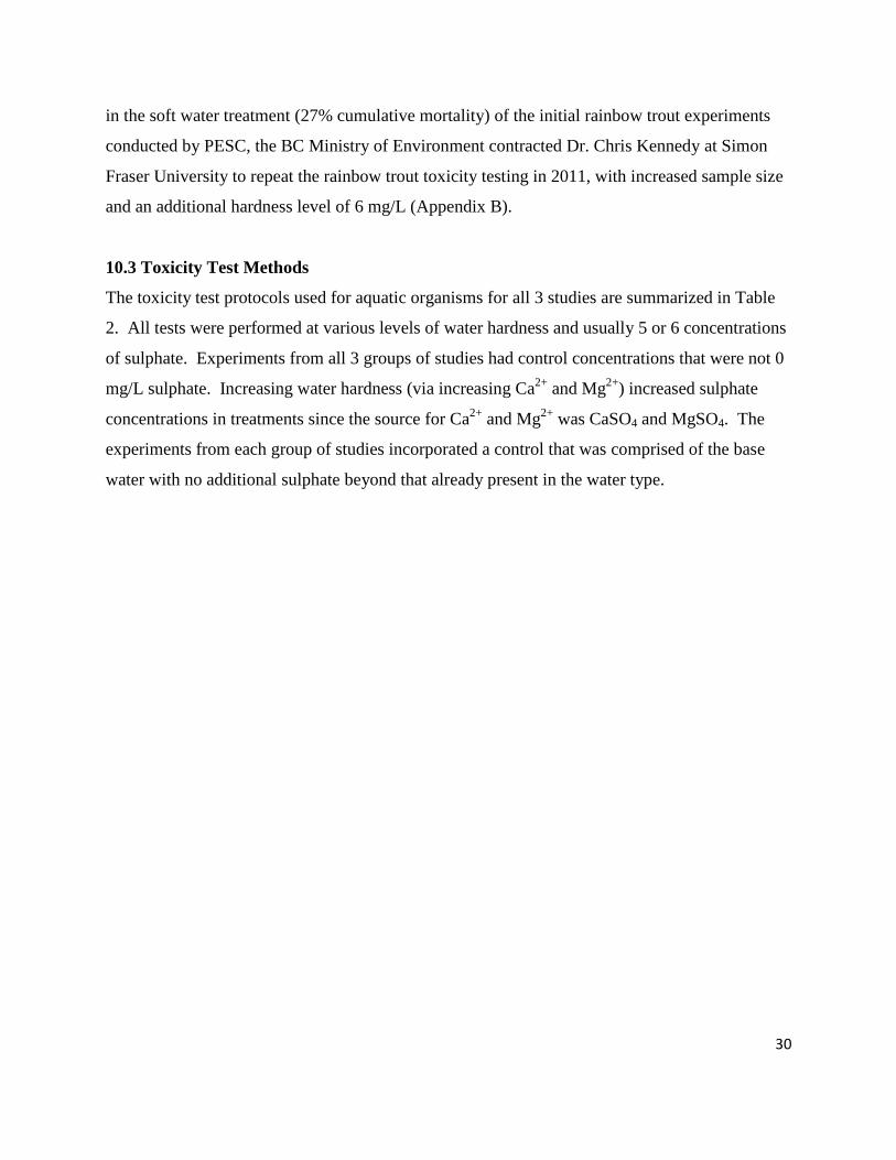
10.3 Toxicity Test Methods

The toxicity test protocols used for aquatic organisms for all 3 studies are summarized in Table

2. All tests were performed at various levels of water hardness and usually 5 or 6 concentrations

of sulphate. Experiments from all 3 groups of studies had control concentrations that were not 0

mg/L sulphate. Increasing water hardness (via increasing Ca2+

and Mg2+

) increased sulphate

concentrations in treatments since the source for Ca2+

and Mg2+

was CaSO4 and MgSO4. The

experiments from each group of studies incorporated a control that was comprised of the base

water with no additional sulphate beyond that already present in the water type.

31

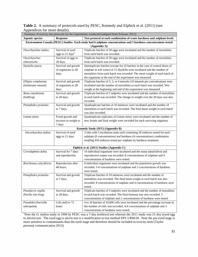
Table 2. A summary of protocols used by PESC, Kennedy and Elphick et al. (2011) (see

Appendices for more details). Summary of toxicity test protocols for the experiments conducted (adapted from Schwarz 2011).

Aquatic species Response Test protocol at each combination of water hardness and sulphate levels

Environment Canada (PESC) Studies- Each study had 6 sulphate concentrations and 3 hardness concentrations tested

(Appendix A)

Oncorhynchus mykiss Survival of eyed

eggs to 21 days1

Triplicate batches of 30 eggs were incubated and the number of mortalities

from each batch was recorded.

Oncorhynchus

tshawytscha

Survival of eggs to

28 days.

Triplicate batches of 30 eggs were incubated and the number of mortalities

from each batch was recorded.

Hyalella azteca Survival and growth

of organisms to 28

days.

Quintuplicate batches (except for 10 batches in the case of control doses of

sulphate in soft water) of 15 Hyalella were incubated and the number of

mortalities from each batch was recorded. The mean weight of each batch of

the organisms at the end of the experiment was measured.

Elliptio complanata

(freshwater mussel)

Survival and growth

of organisms to 28

days.

Triplicate batches of 3, 3, or 4 mussels (10 mussels per concentration) were

incubated and the number of mortalities in each batch was recorded. Wet

weight at the beginning and end of the experiment was measured.

Rana catesbeiana

(bullfrog)

Survival and growth

to 28 days.

Triplicate batches of 5 tadpoles were incubated and the number of mortalities

in each batch was recorded. The change in weight over the 28 days was also

recorded.

Pimephales promelas Survival and growth

to 7 days.

Quadruplicate batches of 10 minnows were incubated and the number of

mortalities in each batch was recorded. The final mean weight in each batch

was also recorded.

Lemna minor Frond growth and

increase in weight to

7 days

Quadruplicate replicates of Lemna minor were incubated and the number of

new fronds and final weight were recorded for each surviving organism.

Kennedy Study (SFU) (Appendix B)

Oncorhynchus mykiss Survival of eyed

eggs to 21 days

3 tubs with 5 incubation units each containing 30 embryos tested for each

sulphate (6 concentrations) and hardness (4 concentrations) combination

totalling 450 embryos tested per sulphate by hardness treatment.

Elphick et al. (2011) Studies (Appendix C)

Ceriodaphnia dubia Survival for 7 days

and reproduction

10 individual organisms were incubated and the status (dead/alive) and

reproductive output was recorded. 8 concentrations of sulphate and 4

concentrations of hardness were tested.

Brachionus calyciflorus Reproduction after

48 hours.

8 individual organisms were incubated and the population growth was

recorded. 5-6 concentrations of sulphate and 3 concentrations of hardness

were tested.

Pimephales promelas Survival and growth

to 7 days.

Triplicate batches of 10 minnows were incubated and the number of

mortalities was recorded. The final mean weight in each batch was also

recorded. 8 concentrations of sulphate and 4 concentrations of hardness were

tested.

Pseudacris regilla

(Pacific tree frog)

Survival and growth

to 28 days.

Triplicate batches of 5 tadpoles were incubated and the number of mortalities

in each batch was recorded. The final biomass was also recorded. 5

concentrations of sulphate and 2 concentrations of hardness were tested.

Pseudokirchneriella

subcapitata

Cell yield to 72

hours

4 to 10 batches of 10,000 cells were incubated and the percentage increase in

the number of cells was recorded. 4-8 concentrations of sulphate and 3

concentrations of hardness were tested. 1Note the O. mykiss study in 1996 by PESC was a 7-day (embryo) test whereas the 2011 study was 21-day (eyed egg

to alevin) test. The eyed egg to alevin test is a modification to test method EPS 1/RM/28. Note the pre-eyed stage is

more sensitive to contaminants than the eyed stage and therefore should be included in toxicity tests (Taylor

personal communication 2013).

32

11.0 Statistical Analysis

Statistical analyses were conducted by Dr. Carl Schwarz (Department of Statistics and Actuarial

Science, Simon Fraser University; Appendices D and E) on the data provided by PESC, Kennedy

and Elphick et al. (2011). Only organisms exposed to at least 2 levels of water hardness were

used for the statistical analysis. When available, effect endpoints were calculated using

measured concentrations.

Maximum likelihood estimation (MLE), a method of estimating the parameters of a statistical

model, was used to fit various models, and to determine if water hardness affected sulphate

toxicity for the species tested. MLE is a standard scientifically-defensible statistical approach for

analyzing toxicity test results (Environment Canada 2007; Appendix D). Due to its

mathematical elegance and ability to account for the control effect in toxicity experiments, MLE

is a preferred approach for statistically analyzing toxicity tests (Environment Canada 2007).

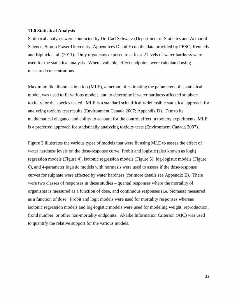
Figure 3 illustrates the various types of models that were fit using MLE to assess the effect of

water hardness levels on the dose-response curve. Probit and logistic (also known as logit)

regression models (Figure 4), isotonic regression models (Figure 5), log-logistic models (Figure

6), and 4-parameter logistic models with hormesis were used to assess if the dose-response

curves for sulphate were affected by water hardness (for more details see Appendix E). There

were two classes of responses in these studies – quantal responses where the mortality of

organisms is measured as a function of dose, and continuous responses (i.e. biomass) measured

as a function of dose. Probit and logit models were used for mortality responses whereas

isotonic regression models and log-logistic models were used for modeling weight, reproduction,

frond number, or other non-mortality endpoints. Akaike Information Criterion (AIC) was used

to quantify the relative support for the various models.

33

Figure 3. Schematic of model types used to estimate sulphate toxicity at different water

hardness. All of the models were fit using the maximum likelihood estimates approach.

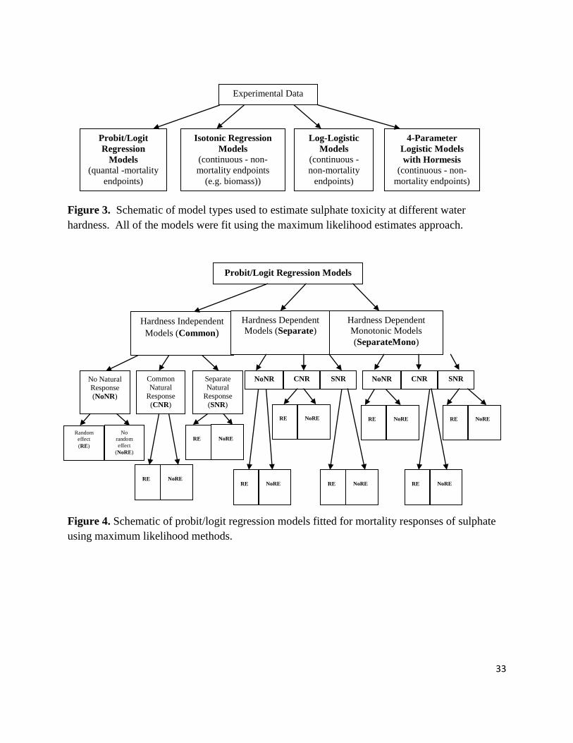
Figure 4. Schematic of probit/logit regression models fitted for mortality responses of sulphate

using maximum likelihood methods.

Probit/Logit

Regression

Models

(quantal -mortality

endpoints)

Experimental Data

Isotonic Regression

Models

(continuous - non-

mortality endpoints

(e.g. biomass))

Log-Logistic

Models

(continuous -

non-mortality

endpoints)

4-Parameter

Logistic Models

with Hormesis

(continuous - non-

mortality endpoints)

Probit/Logit Regression Models

Hardness Independent

Models (Common)

Hardness Dependent

Monotonic Models

(SeparateMono)

Hardness Dependent

Models (Separate)

No Natural Response

(NoNR)

Common

Natural Response

(CNR)

Separate

Natural Response

(SNR)

NoNR

CNR

SNR

NoNR

CNR

SNR

Random

effect

(RE)

No

random

effect

(NoRE)

RE

NoRE

RE

NoRE

RE

NoRE

RE

NoRE

RE

NoRE

RE

NoRE

RE

NoRE

RE

NoRE

34

Figure 5. Schematic of isotonic regression models fitted for continuous responses (e.g. weight,

reproduction etc.) to sulphate using maximum likelihood methods.

Figure 6. Schematic of log-logistic models fitted for continuous responses (e.g. weight,

reproduction etc.) to sulphate using maximum likelihood methods.

11.1 Mortality Responses

Probit and logistic regression models are often suitable for binary response data which assume

that the number of deaths in a toxicity experiment follows a binomial distribution where the

probability of mortality is ‘linked’ to a linear function through the normal distribution in a probit

model or directly on the logistic scale (see Appendix E for details). The probit/logit models were

modified to account for observed mortality at control doses (i.e. non-zero control responses).

This approach allows the control (natural) response rate to be included as another parameter

estimated in the model, rather than assumed to be known from the response observed at the

control doses. Because the control effect (i.e. natural response) estimate is incorporated into the

model, the estimated LCxx values should be interpreted carefully as they will be higher when

compared to the standard reporting of LC values which do not incorporate control mortality.

LCxx values refer to the dose which results in xx% mortality above natural (i.e. control)

mortality. For example, if the control mortality is 13%, 87% of organisms would survive in the

Common curve for all

hardness levels (IR.Common)

Isotonic Regression Models

Separate curve for each

hardness level (IR.Separate)

Common curve for all

hardness levels

(LL3p.Common)

Log-Logistic Models

Separate curve for each

hardness level

(LL3p.Separate)

Monotonic shift to the right in

curves with increasing

hardness levels (LL3p.Mono)

35

absence of sulphate. Therefore the LC25 refers to the additional 25% of 87% that survived (22%

mortality above the control mortality) for a total mortality of 13% + 22% = 35%. In cases where

overdispersion occurred (when data are more variable than expected from a binomial response),

a random-effect probit/logit model was fit to correct for it (see Appendix D for more details).

The effect of water hardness levels on the dose-response curve was tested by fitting 2 (or more)

models to the combined data from the 3 water hardness levels for PESC data, 4 water hardness

levels for Kennedy data, and the 2 to 4 water hardness levels for Elphick et al. (2011) data. The

separate response models used separate probit/logit curves to fit each water hardness level for

each species. The common response models pooled data over all water hardness levels and a

single probit/logit model per species was fit.

The suite of potential probit/logit models fit was described by a 3 part “code” (see Appendix E):

1) Modelling the effects of hardness as either a separate model for each hardness (Separate);

or a common model across all hardness (i.e. hardness independent) (Common); or a

model where increasing hardness is always protective with shifted-to-the-right

(monotonic) dose-response curves as hardness increases (SeparateMono).

2) The model assumes no natural response (NoNR) (i.e. no natural mortality in the control);

a common natural response over all hardness levels (CNR) (i.e. common natural

mortality at the control doses); or a separate natural response for each hardness level

(SNR) (i.e. different mortality at the control doses at each water hardness level tested).

3) The model includes a random effect (RE); or excludes random effects (NoRE) to account

for overdispersion (i.e. more variation than expected).

For example, a probit/logit model identified as Common, NoNR, NoRE corresponds to fitting the

model with a common curve across all hardness levels, no natural responses, and no random

effects.

11.2 Continuous Responses

There is no common model suitable for modeling weight, reproduction, frond number, or other

36

continuous endpoints. Although the CETIS software offers a suite of potential models, in the

majority of the cases, the program most often applies a linear interpolation method (ICPIN) also

known as isotonic regression (Barlow et al. 1972). The basic premise is that the response

variable (i.e. weight, reproduction etc.) should decline with increasing sulphate levels. Schwarz

(Appendices D and E) used the maximum likelihood approach under monotonicity for the non-

parametric isotonic regression. This method can be used with mortality data if there is evidence

of a structural lack of fit in the probit/logit model, however, the LCxx values from isotonic

regression are not directly comparable to those from the maximum likelihood probit/logit

approach with natural response (i.e. control mortality) incorporated. With the isotonic regression

method, no natural response is assumed (i.e. no control mortality), therefore, LCxx values based

on CETIS output sheets using ICPIN should not be directly compared.

Estimates of the ICxx values were estimated by linear interpolation on the log(dose) scale. ICxx

responses were measured from the mean response at the lowest observable dose rather than at

dose 0. For example, if a study used doses 100, 200, 400, 800, 1,600 for sulphate, the baseline

response is estimated from the dose 100 mean. Starting doses were not consistent for different

water hardness levels, therefore baseline response may differ among these studies solely because

of different initial doses and not because of water hardness effects. Standard errors (and

confidence limits) for the ICxx values are found using a bootstrap method. Several hundred

bootstrap samples were generated with replacement from the observed data. For each bootstrap

sample, the isotonic regression model was fit and the estimate of the ICxx value determined.

The 2.5th

and 97.5th

percentile of the bootstrap estimates were used as the 95% confidence

intervals for the parameter. Note that ICxx values that exceed the largest dose observed in the

experiment cannot be estimated because there is no information from the data on the shape of the

curve after the largest observed dose. In these cases, no estimate was reported. Similarly, in

some cases, the isotonic regression line was completely flat and no estimate of the ICxx values

could be computed.

Isotonic regression models were fit where a single curve was common for all hardness levels

(denoted as IR.Common) or a separate curve was fit for each hardness level (IR.Separate).

37

Three log-logistic models were also fit. The LL3p.Common model which assumed a common

curve over all hardness levels; the LL3p.Separate model which assumed a separate curve for

each hardness level; and the LL3p.Mono model which assumed a shift in the curves to the right

with increasing hardness levels.

Two other models (4-parameter logistic model with hormesis) were fit for some responses where

there was evidence of an increase in response at lower doses. The LH4p.Common model

assumed a common curve over all hardness levels; the LH4p.Separate model assumed a separate

curve for each hardness level.

11.3 Model Ranking and Fitting

Schwarz (see Appendix E) used Akaike Information Criterion (AIC) to compare and rank the

fitted models for the species and endpoints datasets. It is recognized that all models are only

approximations to reality and the relative support among the models is computed to rank the

models. The AIC corrected for small sample sizes (AICc) was used to rank the models. AICc

measures the tradeoff between model complexity (number of parameters) and model fit

(likelihood value). The difference in AICc (ΔAICc) between the best fitting model and the other

models is a measure of how similar 2 models are in the fit-complexity trade-off. AICc only

looks at the models in the set and does not assess whether the model adequately fits the data,

therefore a visual inspection of the results needs to be conducted and goodness-of-fit statistics

need to be assessed.

11.4 Model Averaging and Calculation of Benchmark Dose

Many different statistical models may fit toxicity data and the choice of model can influence the

value of the endpoint calculated from toxicity studies. In general, smaller endpoints are very

sensitive to the models used, and therefore one of the dangers of reporting only a single value

from a single “best fitting model” is that minor changes to the data and/or different models that

fit the data equally well, can lead to very different estimates (Schwarz, personal communication

2011). Model averaging is a method used to determine the relative support of various models

about the effect of water hardness on the dose-response curve and toxicity of different levels of

38

sulphate to aquatic organisms. Model averaging was used to calculate the benchmark dose

(BMD) such as the LCxx (dose at which xx% additional mortality occurs over control natural

mortality) or ICxx (dose at which the response (e.g. weight) is reduced from control).

The estimates of BMDs are model-based because direct estimation off a curve would require

using several hundreds or thousands of organisms at a wide range of doses (see Appendix E).

Typically BMD has been estimated by choosing one of many dose-response curves that fit the

toxicity data collected. Software such as CETIS provide a large number of dose-response curves

(models) that can be fit to the same dataset; however each curve can lead to a different estimate

of BMD. The analyst must choose which model should be used amongst the various models that

fit the data. They may choose the model that is the “best” fitting or they may decide to choose

the model that gives more conservative or liberal estimates. Choosing one model can be

problematic in that: 1) slight changes to the dataset could lead to different models fitting the data;

2) selecting the “best fitting” model depends on the criteria used to define the fit of the model

and different criteria could lead to different choices of the best model; 3) risk estimates derived

from similarly fitting models may be substantially different especially at the lower bound

estimates; and 4) choosing one model does not incorporate model uncertainty which can be an

important part in risk assessment (Bailer et al. 2005; Appendix E).

Model weights provide a way to combine estimates over competing models. Each model

provides an estimate of LCxx and a weighted average (based on the model weight) - the "best"

guess for this parameter. The standard errors from each model are also averaged. Additionally,

if the estimates of LCxx vary considerably among models, an extra component of variation to

account for this variation in estimates of LCxx is also included. Model averaging “averages” the

BMD based on the support each model provides in the data (see Appendices D and E). AICc,

ΔAICc and model weight were all used to calculate estimates and confidence intervals for

LCxx/ECxx/ICxx from the PESC, Kennedy and Elphick et al. (2011) data (Tables 3, 4 and 5,

respectively). Appendix E gives summaries of AIC model selection for each species and data

set. Support (model weight) for models ranged from 0.0 (no support) to 1.0 (strong support), and

varied across and within aquatic species, depending on the endpoint measured. Model averaging

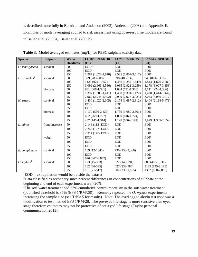
39

is described more fully in Burnham and Anderson (2002), Anderson (2008) and Appendix E.

Examples of model averaging applied to risk assessment using dose-response models are found

in Bailer et al. (2005a), Bailer et al. (2005b).

Table 3. Model-averaged estimates (mg/L) for PESC sulphate toxicity data.

Species Endpoint Water

Hardness

LC10/ EC10/IC10

(CI)

LC25/EC25/IC25

(CI)

LC50/EC50/IC50

(CI)

O. tshawytscha survival 50 EOD1 EOD EOD

100 EOD EOD EOD

250 1,287 (1,028-1,610) 2,521 (1,807-3,517) EOD

P. promelas2 survival 50 379 (283-506) 598 (489-732) 946 (801-1,116)

100 1120 (924-1,357) 1,436 (1,252-1,649) 1,843 (1,626-2,089)

250 3,092 (2,666-3,586) 3,085 (2,921-3,259) 3,178 (3,007-3,358)

biomass 50 931 (666-1,301) 1,004 (771-1,308) 1,111 (924-1,336)

100 1,397 (1,383-1,411) 1,408 (1,394-1,422) 1,428 (1,414-1,442)

250 2,969 (2,946-2,992) 2,999 (2,975-3,023) 3,053 (3,030-3,077)

H. azteca survival 50 1,430 (1,020-2,005) 2,178 (1,687-2,812) 3,404 (2,118-5,471)

100 EOD EOD EOD

250 EOD EOD EOD

biomass 50 1,170 (566-2,420) 1,739 (1,080-2,801) EOD

100 682 (269-1,727) 1,030 (616-1,724) EOD

250 437 (145-1,314) 1,198 (656-2,191) 1,929 (1,305-2,852)

L. minor2 frond increase 50 2,143 (112- EOD) EOD EOD

100 2,243 (127- EOD) EOD EOD

250 2,314 (147- EOD) EOD EOD

weight 50 EOD EOD EOD

100 EOD EOD EOD

250 EOD EOD EOD

E. complanata survival 50 139 (12-1640) 730 (158-3,360) EOD

100 EOD EOD EOD

250 676 (367-6,842) EOD EOD

O. mykiss3 survival 50 123 (45-333) 322 (149-694) 889 (408-1,936)

100 162 (66-395) 427 (233-780) 1189 (645-2,189)

250 191 (71-517) 502 (239-1,055) 1392 (668-2,898) 1EOD = extrapolation would be outside the dataset

2Data classified as secondary since percent differences in concentrations of sulphate at the

beginning and end of each experiment were >20%. 3The soft water treatment had 27% cumulative control mortality in the soft water treatment

(published threshold is 35% (EPS 1/RM/28)). Kennedy repeated the O. mykiss experiments

increasing the sample size (see Table 5 for results). Note: The eyed egg to alevin test used was a

modification to test method EPS 1/RM/28. The pre-eyed life stage is more sensitive than eyed

stage therefore estimates may not be protective of pre-eyed life stage (Taylor personal

communication 2013).

40

Table 4. Model averaged estimates (mg/L) for Kennedy’s 21-d rainbow trout early life stage1

sulphate toxicity data (see Appendix B for more information).

Species Endpoint Water

Hardness

LC10 (CI) LC20 (CI) LC50 (CI)

O. mykiss survival 6 176 (161 – 192) 255 (238 – 274) 484 (459 – 511)

50 315 (290 – 341) 435 (408 – 464) 761 (724 – 799)

100 444 (409 – 482) 618 (580 – 659) 1,093 (1,037 – 1,151)

250 654 (615 – 695) 857 (819 – 896) 1,379 (1,329 – 1,433) 1 Note: The eyed egg to alevin test used was a modification to test method EPS 1/RM/28. The

pre-eyed life stage is more sensitive than eyed stage therefore estimates may not be protective of

pre-eyed life stage (Taylor personal communication 2013).

Table 5. Model averaged estimates1 (mg/L) for Elphick et al. (2011) sulphate toxicity data.

Species Endpoint Water

Hardness

LC10/ EC10/IC10 (CI) LC25/EC25/IC25 (CI) LC50/EC50/IC50 (CI)

C. dubia survival 40 402 (279 – 581) 570 (419 – 775) 809 (612 – 1,071)

80 593 (382 – 920) 871 (628 – 1,208) 1,282 (962 – 1,708)

160 857 (594 – 1,237) 1,145 (872 – 1,504) 1,531 (1,189 – 1,972)

320 816 (609 – 1,095) 1,135 (884 – 1,456) 1,580 (1,236 – 2,019)

reproduction 40 158 (11 – 2,331) 272 (61 – 1,215) 468 (217 – 1009)

80 708 (356 – 1,409) 890 (578 – 1,369) 1,119 (911– 1,374)

160 1,184 (1,166 – 1,203) 1,223 (1,213 – 1,233) 1,263 (1,253 – 1,273)

320 253 (53 – 1210) 425 (144 – 1257) 717 (343 – 1,498)

B. calyciflorus reproduction 40 733 (41 – EOD2) 995 (597 – 1,660) 1,211 (759 – 1,933)

80 352 (63 – 1,969) 1,799 (933 – 3,469) 2,191 (840 – 5,717)

160 724 (341 – 1,536) 1,311 (209 – EOD) EOD

320 848 (177 – 4,059) 1,071 (299 – 3,837) EOD

P. promelas survival 40 352 (241 – 515) 743 (558 – 988) 1,565 (1,199 – 2,041)

80 464 (316 – 681) 1043 (786 – 1,384) 2,344 (1,751 – 3,137)

160 1,244 (853 – 1,815) 2,549 (1,898 – 3,423) 5,222 (3,649 – 7,472)

320 2,516 (1,548 – 4,089) 6376 (2,910 - EOD) EOD

biomass 40 600 (346 – 1,038) 869 (612 – 1,233) 1,260 (979 – 1,621)

80 1,330 (930 – 1,904) 1,845 (1,421 – 2,396) 2,559 (2,018 – 3,244)

160 2,102 (1,246 – 3,548) 2,809 (1,932 – 4,083) 3,752 (2,528 – 5,568)

320 EOD2 716 (EOD) 4,304 (1,584-EOD)

P. regilla survival 15 587 (256 – 1,346) 1,068 (645 – 1,769) 1,986 (1,212 – 3,255)

80 242 (90 – 646) 607 (328 – 1,124) 1,583 (845 – 2,964)

biomass 15 1,246 (138-EOD) 1,441 (191-EOD) 1,828 (1,744-1,917)

80 1,276 (671-2429) 1,385 (860-2231) 1,577 (1184-2100)

P. subcapitata cell yield 10 441 (196-988) 696 (415-1,168) 1,101 (821-1,477)

80 2,487 (2,300-2,690) 2,615 (2,500-2,736) 2,749 (2,701-2,798)

320 2,548 (2,464-2,634) 2,660 (2,618-2,702) 2,777 (2,744-2,810) 1Data classified as secondary since concentrations of sulphate were not measured for each

treatment at a minimum at the beginning and end of each experiment. 2EOD = extrapolation would be outside the dataset

41

12.0 Results

Models with separate dose-response curves for each water hardness level were given the

majority of model weight in the analyses in all but 3 cases (Appendices D and E). For L. minor

frond numbers and L. minor weight there was strong support (AICc weight of 0.62, and 0.66,

respectively) for models where the dose-response curve was invariant across water hardness;

however, many estimates for L. minor weight could not be determined as extrapolation would be

outside the dataset. The natural variation and limited response to sulphate made it difficult to

determine the effect of hardness on the dose-response curve. For the PESC rainbow trout

mortality data, support was very close between two models, with a model that was invariant to

water hardness being slightly more supported (AICc weight 0.49) than the model where the

dose-response curve was “protective” as water hardness increased from 50 to 250 mg/L (AICc

weight 0.40). While there was some support for water hardness to be protective to the rainbow

trout eyed embryo to alevin stage, the protection was minor (e.g. 21-day LC10 of 123, 162, and

191 mg/L SO42-

at 50, 100, and 250 mg/L water hardness; Table 4). In the second test conducted

on rainbow trout eyed embryo to alevin by Kennedy in 2011, support was very strong (AICc

weight 1.0) for the logit H*D model where the dose-response curve was “protective” as water

hardness increased. Fathead minnow had similar support for models where the dose-response

curves were different across water hardness levels (AICc weights of 0.36 and 0.45 for mortality

and weight, respectively) and models where the dose-response curve shifts monotonically (i.e.

always more protective) as hardness increases (AICc weights of 0.64 and 0.55 for mortality and

weight, respectively). The Pacific tree frog became more sensitive to sulphate by increasing

water hardness from 15 to 80 mg/L (28-day LC10 of 587 (256-1,346) mg/L to 28-day LC10 of

242 (90-646) mg/L, respectively). Other species (e.g. Ceriodaphnia and Brachionus) showed

decreases and increases in toxicity with increasing water hardness depending on the levels

compared.

Of the species tested, the most sensitive species and endpoints were: rainbow trout eyed embryo

to alevin survival at 6 mg/L water hardness with a 21-day LC10 of 176 (161 – 192) mg/L;

Pacific tree frog tadpoles survival at 80 mg/L water hardness with a 28-day LC10 of 242 (90 –

646) mg/L; Ceriodaphnia dubia reproduction at water hardness of 40 mg/L and 320 mg/L with

42

LC 10 of 158 (11-2,331) mg/L and 253 (53-1,210) mg/L, respectively; fathead minnow 7-day

survival in soft water 7-day LC10 of 352 (241-515) mg/L at 40 mg/L hardness (from Elphick et

al. 2011 data analysis) and 7-day LC10 of 379 (283-506) mg/L at 50 mg/L water hardness (from

PESC data); and E. complanata (freshwater mussel) survival 28-day LC10 of 139 (12 – 1640)

mg/L at 50 mg/L hardness.

The rainbow trout eyed embryo to alevin test (which measures multiple phases of development)

appears to be a sensitive endpoint and was much more sensitive than values reported for the

embryo stage of chinook or coho salmon (Elphick et al. 2011; PESC; Kennedy). The 21-day

eyed embryo to alevin test for rainbow trout was also more sensitive than the 7-day LC50

embryo test ((E) test), often used for routine monitoring) conducted by PESC in 1996 (Singleton

2000). However, the eyed egg to alevin test used was a modification to test method EPS

1/RM/28. Taylor (personal communication 2013) stated that the pre-eyed life stage would be a

more sensitive endpoint.

Observed mortality in chinook eggs from the PESC data was so low that no model was able to

provide sensible estimates of the LCxx values for lower hardness levels. Note that C. dubia

reproduction, Pacific treefrog survival and biomass, and E. complanata survival had large

confidence intervals associated with their estimates.

13.0 Discussion and Application of the Sulphate Guidelines

Many factors appear to affect sulphate toxicity. These include the test organism used; the test

duration, the endpoint (mortality, growth, behaviour, reproduction etc.), the test water chemistry,

and the statistical model chosen to analyse the data. It is difficult to distinguish quantitative

relationships that apply broadly with respect to these factors; therefore caution must be exercised

when developing generic water quality guidelines.

When setting an ambient water quality guideline it is important to determine whether to set a

single value or multiple values related to modifying factors such as water hardness or other

factors. Many studies in the literature concluded that water hardness (or TDS or conductivity)

43

has an effect on the toxicity of sulphate to aquatic organisms (Soucek and Kennedy 2005;

Soucek 2007a; Lewis et al. 2007; Davies 2007; Lasier and Hardin 2010; Elphick et al. 2011).

Although for most of the endpoints tested by PESC, Kennedy, and Elphick et al. (2011), the

majority of the model weights were given to models where the dose-response curve is different

at the different hardness levels tested; there was no consistent ameliorative effect between

sulphate toxicity and water hardness identified. Similarly to Elphick et al. (2011), Schwarz

(Appendices D and E) failed to find a consistent relationship between water hardness and

sulphate toxicity for aquatic species, or within aquatic species for different endpoints. For some

species and endpoints, the inability to distinguish between sulphate toxicity dose-response curves

for different water hardness levels may be due to the low power associated with a small number

of organisms tested or high variability in responses (i.e. large confidence intervals). In 2011,

Kennedy repeated the rainbow trout experiment conducted by PESC, increasing the sample size

which resulted in toxicity estimates that had much narrower confidence intervals. The Kennedy

study showed that the toxicity of sulphate to rainbow trout early life stages was ameliorated by

increased water hardness to 250 mg/L (highest hardness tested). Increased sample size in future

studies could help to decrease variability associated with estimates for other species, and trends

may become clearer for species that showed high variability. It would be useful in future studies

to conduct a power analysis to help determine the samples sizes needed to detect biological

differences in the endpoints.

The effect of water hardness may differ depending on the concentration, organism, and endpoint

investigated. Most of the organisms tested did not show strong support for the model with

monotonicity (i.e. always a progressively protective effect of increasing water hardness).

However, the most sensitive species tested was rainbow trout (the 21-d eyed embryo to alevin

life stage) which demonstrated some amelioration of sulphate toxicity with increasing water

hardness from 6 mg/L up to 250 mg/L. As a result the long-term average sulphate guideline was

developed for different categories of water hardness based on the rainbow trout LC20 data with

the minimum uncertainty factor of 2 applied. Figure 7 shows the 30-day average sulphate

guideline along with the model averaged rainbow trout toxicity data from the Kennedy study.

Figure 8 shows the sulphate guideline graphed with all the model averaged toxicity estimates for

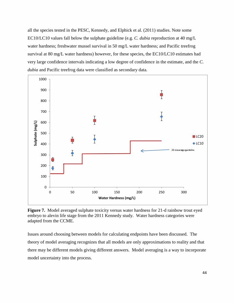
44

all the species tested in the PESC, Kennedy, and Elphick et al. (2011) studies. Note some

EC10/LC10 values fall below the sulphate guideline (e.g. C. dubia reproduction at 40 mg/L

water hardness; freshwater mussel survival in 50 mg/L water hardness; and Pacific treefrog

survival at 80 mg/L water hardness) however, for these species, the EC10/LC10 estimates had

very large confidence intervals indicating a low degree of confidence in the estimate, and the C.

dubia and Pacific treefrog data were classified as secondary data.

Figure 7. Model averaged sulphate toxicity versus water hardness for 21-d rainbow trout eyed

embryo to alevin life stage from the 2011 Kennedy study. Water hardness categories were

adapted from the CCME.

Issues around choosing between models for calculating endpoints have been discussed. The

theory of model averaging recognizes that all models are only approximations to reality and that

there may be different models giving different answers. Model averaging is a way to incorporate

model uncertainty into the process.

0

100

200

300

400

500

600

700

800

900

1000

0 50 100 150 200 250 300

Sulp

hat

e (

mg/

L)

Water Hardness (mg/L)

LC20

LC10

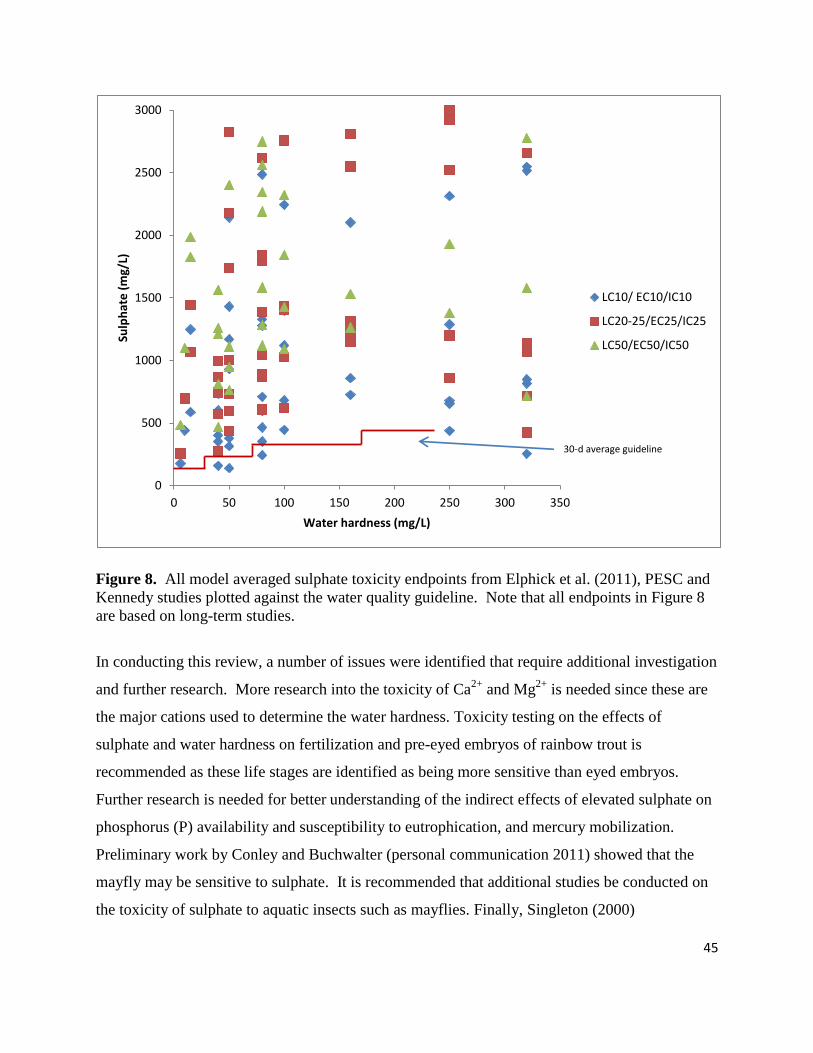
45

Figure 8. All model averaged sulphate toxicity endpoints from Elphick et al. (2011), PESC and

Kennedy studies plotted against the water quality guideline. Note that all endpoints in Figure 8

are based on long-term studies.

In conducting this review, a number of issues were identified that require additional investigation

and further research. More research into the toxicity of Ca2+

and Mg2+

is needed since these are

the major cations used to determine the water hardness. Toxicity testing on the effects of

sulphate and water hardness on fertilization and pre-eyed embryos of rainbow trout is

recommended as these life stages are identified as being more sensitive than eyed embryos.

Further research is needed for better understanding of the indirect effects of elevated sulphate on

phosphorus (P) availability and susceptibility to eutrophication, and mercury mobilization.

Preliminary work by Conley and Buchwalter (personal communication 2011) showed that the

mayfly may be sensitive to sulphate. It is recommended that additional studies be conducted on

the toxicity of sulphate to aquatic insects such as mayflies. Finally, Singleton (2000)

0

500

1000

1500

2000

2500

3000

0 50 100 150 200 250 300 350

Sulp

hat

e (

mg/

L)

Water hardness (mg/L)

LC10/ EC10/IC10

LC20-25/EC25/IC25

LC50/EC50/IC50

30-d average guideline

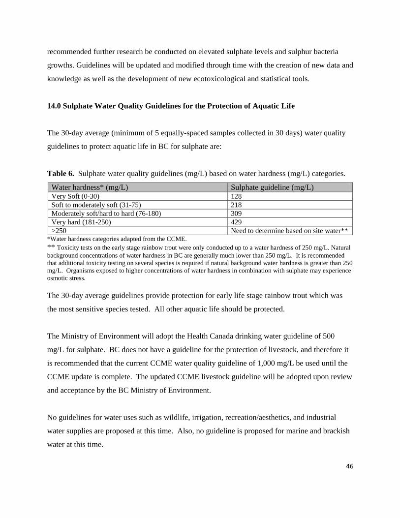
46

recommended further research be conducted on elevated sulphate levels and sulphur bacteria

growths. Guidelines will be updated and modified through time with the creation of new data and

knowledge as well as the development of new ecotoxicological and statistical tools.

14.0 Sulphate Water Quality Guidelines for the Protection of Aquatic Life

The 30-day average (minimum of 5 equally-spaced samples collected in 30 days) water quality

guidelines to protect aquatic life in BC for sulphate are:

Table 6. Sulphate water quality guidelines (mg/L) based on water hardness (mg/L) categories.

Water hardness* (mg/L) Sulphate guideline (mg/L) Very Soft (0-30) 128 Soft to moderately soft (31-75) 218 Moderately soft/hard to hard (76-180) 309 Very hard (181-250) 429 >250 Need to determine based on site water**

*Water hardness categories adapted from the CCME.

** Toxicity tests on the early stage rainbow trout were only conducted up to a water hardness of 250 mg/L. Natural

background concentrations of water hardness in BC are generally much lower than 250 mg/L. It is recommended

that additional toxicity testing on several species is required if natural background water hardness is greater than 250

mg/L. Organisms exposed to higher concentrations of water hardness in combination with sulphate may experience

osmotic stress.

The 30-day average guidelines provide protection for early life stage rainbow trout which was

the most sensitive species tested. All other aquatic life should be protected.

The Ministry of Environment will adopt the Health Canada drinking water guideline of 500

mg/L for sulphate. BC does not have a guideline for the protection of livestock, and therefore it

is recommended that the current CCME water quality guideline of 1,000 mg/L be used until the

CCME update is complete. The updated CCME livestock guideline will be adopted upon review

and acceptance by the BC Ministry of Environment.

No guidelines for water uses such as wildlife, irrigation, recreation/aesthetics, and industrial

water supplies are proposed at this time. Also, no guideline is proposed for marine and brackish

water at this time.

47

15.0 Literature Cited

Agriculture and Agri-Food Canada (AAFC). 2012. Water quality and Cattle.

http://www4.agr.gc.ca/AAFC-AAC/display-afficher.do?id=1187377614629&lang=eng

(accessed May 14, 2012).

American Public Health Association/American Water Works Association/Water Pollution

Control Federation (APHA). 1985. Standard Methods for the examination of water and

wastewater. 16th edition. APHA, Washington DC.

Anderson, D. 2008. Model Based Inference in the Life Sciences: A Primer on Evidence.

Springer: New York. 184 p.

Arthur D. Little Inc. 1971. Water Quality Criteria Data Book. Vol. 2. Inorganic chemical

pollution of freshwater. Water Pollut. Control Res. Ser. No. DPV 18010, US EPA,

Washington, DC. Cited from Health Canada, 1996.

Australian Government. 2004. Australian Drinking Water Guidelines.

http://www.nhmrc.gov.au/guidelines/publications/eh34 (accessed April 19, 2012).

Bailer, A.J., M. Wheeler, D. Dankovick, R. Noble, and J. Bena. 2005a. Incorporating

uncertainty and variability in the assessment of occupational hazards. Int. J Risk Assess.

Manage 5:344–357.

Bailer, A.J., R. Noble, and M. Wheeler. 2005b. Model uncertainty and risk estimation for

experimental studies of quantal responses. Risk Analysis 25: 291-299.

BC MoE 2012. Derivation of water quality guidelines to protect aquatic life in British

Columbia. Water Protection and Sustainability Branch. Environmental Sustainability and

Strategic Policy Division. Ministry of Environment. 34 p.

Borgmann, U. 1996. Systematic analysis of aqueous ion requirements of Hyalella azteca: a

standard artificial medium including the essential bromide ion. Arch. Environ. Contamin.

Toxicol. 30:356-363.

Brouwer, E. J. Soontiëns, R. Bobbink and J.G.M.Roelofs. 1999. Sulphate and bicarbonate as

key factors in sediment degradation and restoration of Lake Banen. Aquatic Conserv. Mar.

Freshw. Ecosyst. 9:121-132.

Buday, C. (personal communication). 2010. Environmental Toxicology Section, Pacific

Environmental Science Centre, Environment Canada 2645 Dollarton Highway North

Vancouver, BC

48

Burnham, K.P. and D. R. Anderson. 2002. Model selection and multi-model inference: a

practical information-theoretic approach. Springer, New York.

Canadian Council of Ministers of the Environment (CCME). 2007. A Protocol for the

Derivation of Water Quality Guidelines for the Protection of Aquatic Life. Canadian

Environmental Quality Guidelines. 37 p.

http://ceqg-rcqe.ccme.ca/?config=ccme&thesite=ceqg&words=&image.x=0&image.y=0

Conley, J, N. Cariello and D. Buchwalter. 2010. Preliminary investigations of TDS toxicity and

sulfate trafficking in mayflies. PowerPoint presentation. Presented at SETAC, November 7-

11, 2010. Portland, OR.

Conley and Buchwalter (personal communication) 2011. Department of Environmental and

Molecular Toxicology, North Carolina State University. Raleigh, NC. February 9, 2011.

Curtis, P.J. 1989. Effects of hydrogen ion and sulfate on the phosphorus cycle of a Precambrian

Shield lake. Nature 337:156-158.

Davies, T. D. 2002. Sulphate toxicity to freshwater organisms and molybdenum toxicity to

rainbow trout (Oncorhynchus mykiss). Master of Science Thesis, Resource Management and

Environmental Studies. University of British Columbia. 119p.

Davies, T. D., and K. J. Hall. 2007. Importance of calcium in modifying the acute toxicity of

sodium sulphate to Hyalella azteca and Daphnia magna. Environm. Toxicol. and Chem.

26:1243-1247.

Davies, T. D. 2007. Sulphate toxicity to the aquatic moss, Fontinalis antipyretica.

Chemosphere. 66: 444-451.

Dowden, B.F. and H.J. Bennett. 1965. Toxicity of selected chemicals to certain animals. J.

Water Pollut. Control Fed. 37(9):1308-1316.

Drinking Water Leadership Council. 2007. Drinking Water Officers’ Guide. Available online

at http://www.health.gov.bc.ca/protect/dwpublications.html

Elphick, J.R., M. Davies, G. Gilron, E. C Canaria, B. Lo and H. C Bailey. 2011. An aquatic

toxicological evaluation of sulfate: The case for considering hardness as a modifying factor in

setting water quality guidelines. Environ. Toxicol. Chem. 30(1):247-53.

Environment Canada. 1984. Detailed surface water quality data, Northwest Territories 1980-

1981, Alberta 1980-1981, Saskatchewan 1980-1981. Manitoba 1980-1981. Unpublished

results provided by Inland Waters Directorate, Ottawa. Cited from Health Canada, 1996.

Environment Canada. 1997. Biological Test Method: Test for Survival and Growth in

Sediment Using the Freshwater Amphipod Hyalella azteca, Report EPS 1/RM/33.

49

Environment Canada. 2007. Guidance Document on Statistical Methods for Environmental

Toxicity Tests. Report EPS 1/RM/46. Methods Development and Applications Section.

Environmental Toxicology Centre. Ottawa, ON. 241 p.

Fenchel, T., G.M. King, and T.H. Blackburn. 2000. Bacterial Biogeochemistry The

Ecophysiology of Mineral Cycling. Academic Press. London, UK. 307 p.

Fingl E. 1980. Laxatives and cathartics. In: Pharmacological basis of therapeutics. A.G. Gilman

and L. Gilman (eds.) McMillan Publishing Co. New York. Cited from Health Canada, 1996.

Frahm, J.P. 1975. Toxicity tolerance studies utilizing periphyton. (Toxitoleranzversuche an

Wassermoosen). Gewasser Und Abwasser 57/58:59-66.

Geurts J.J.M., J. M. Sarneel, B. J.C. Willers, J. G.M. Roelofs, J. T.A. Verhoeven, and L.P.M.

Lamers 2009. Interacting effects of sulphate pollution, sulphide toxicity and eutrophication

on vegetation development in fens: A mesocosm experiment. Environmental Pollution

157:2072–2081.

Gilli, G. and P. M. Comune. 1980. Effetti della salinità su sistemi biologici. Inquinamento

22(100):31-35.

Goetsch, P.A., and C. G. Palmer. 1997. Salinity Tolerances of Selected Macroinvertebrates of

the Sabie River, Kruger National Park, South Africa. Arch. Environ. Contam. Toxicol.

32:32–41.

Goodfellow, W.L., L.W. Ausley, D.T. Burton, D.L Denton, P.B Dorn, D.R Grothe, M.A., Heber,

T.J Norberg-King, and J.H Rodgers Jr. 2000. Major ion toxicity in effluents: a review with

permitting recommendations. Environ. Toxicol. Chem. 19:175–182.

Han, S., A. Obraztsova, P. Pretto, K-Y Choe, J. Gieskes, D. D. Deheyn, and B. M. Tebo. 2007.

Biogeochemical factors affecting mercury methylation in sediments of the Venice lagoon,

Italy. Environm. Toxicol. and Chem. 26, No. 4: 655– 663.

Harmon, S.M., J.K. King, J.B. Gladden, G.T. Chandler, and L.A. Newman. 2004.

Methylmercury formation in a wetland mesocosm amended with sulfate. Environm. Sci. and

Tech. 38:650-656.

Health Canada. 1996. Guidelines for Canadian Drinking Water Quality, Part II: Supporting

Documentation. Ottawa.

Health Canada. 2010. Guidelines for Canadian Drinking Water Quality Summary Table.

Federal-Provincial-Territorial Committee on Drinking Water. Federal-Provincial-Territorial

Committee on Health and the Environment. Ottawa, Canada. December 2010.

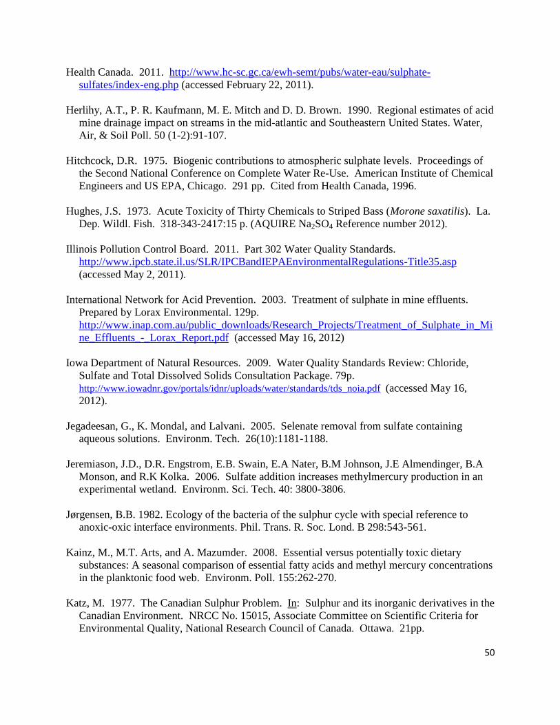
50

Health Canada. 2011. http://www.hc-sc.gc.ca/ewh-semt/pubs/water-eau/sulphate-

sulfates/index-eng.php (accessed February 22, 2011).

Herlihy, A.T., P. R. Kaufmann, M. E. Mitch and D. D. Brown. 1990. Regional estimates of acid

mine drainage impact on streams in the mid-atlantic and Southeastern United States. Water,

Air, & Soil Poll. 50 (1-2):91-107.

Hitchcock, D.R. 1975. Biogenic contributions to atmospheric sulphate levels. Proceedings of

the Second National Conference on Complete Water Re-Use. American Institute of Chemical

Engineers and US EPA, Chicago. 291 pp. Cited from Health Canada, 1996.

Hughes, J.S. 1973. Acute Toxicity of Thirty Chemicals to Striped Bass (Morone saxatilis). La.

Dep. Wildl. Fish. 318-343-2417:15 p. (AQUIRE Na2SO4 Reference number 2012).

Illinois Pollution Control Board. 2011. Part 302 Water Quality Standards.

http://www.ipcb.state.il.us/SLR/IPCBandIEPAEnvironmentalRegulations-Title35.asp

(accessed May 2, 2011).

International Network for Acid Prevention. 2003. Treatment of sulphate in mine effluents.

Prepared by Lorax Environmental. 129p.

http://www.inap.com.au/public_downloads/Research_Projects/Treatment_of_Sulphate_in_Mi

ne_Effluents_-_Lorax_Report.pdf (accessed May 16, 2012)

Iowa Department of Natural Resources. 2009. Water Quality Standards Review: Chloride,

Sulfate and Total Dissolved Solids Consultation Package. 79p.

http://www.iowadnr.gov/portals/idnr/uploads/water/standards/tds_noia.pdf (accessed May 16,

2012).

Jegadeesan, G., K. Mondal, and Lalvani. 2005. Selenate removal from sulfate containing

aqueous solutions. Environm. Tech. 26(10):1181-1188.

Jeremiason, J.D., D.R. Engstrom, E.B. Swain, E.A Nater, B.M Johnson, J.E Almendinger, B.A

Monson, and R.K Kolka. 2006. Sulfate addition increases methylmercury production in an

experimental wetland. Environm. Sci. Tech. 40: 3800-3806.

Jørgensen, B.B. 1982. Ecology of the bacteria of the sulphur cycle with special reference to

anoxic-oxic interface environments. Phil. Trans. R. Soc. Lond. B 298:543-561.

Kainz, M., M.T. Arts, and A. Mazumder. 2008. Essential versus potentially toxic dietary

substances: A seasonal comparison of essential fatty acids and methyl mercury concentrations

in the planktonic food web. Environm. Poll. 155:262-270.

Katz, M. 1977. The Canadian Sulphur Problem. In: Sulphur and its inorganic derivatives in the

Canadian Environment. NRCC No. 15015, Associate Committee on Scientific Criteria for

Environmental Quality, National Research Council of Canada. Ottawa. 21pp.

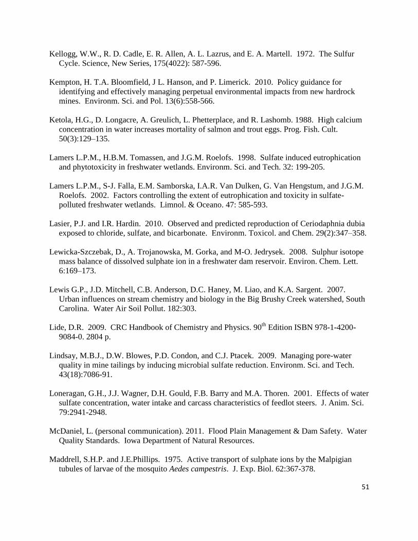
51

Kellogg, W.W., R. D. Cadle, E. R. Allen, A. L. Lazrus, and E. A. Martell. 1972. The Sulfur

Cycle. Science, New Series, 175(4022): 587-596.

Kempton, H. T.A. Bloomfield, J L. Hanson, and P. Limerick. 2010. Policy guidance for

identifying and effectively managing perpetual environmental impacts from new hardrock

mines. Environm. Sci. and Pol. 13(6):558-566.

Ketola, H.G., D. Longacre, A. Greulich, L. Phetterplace, and R. Lashomb. 1988. High calcium

concentration in water increases mortality of salmon and trout eggs. Prog. Fish. Cult.

50(3):129–135.

Lamers L.P.M., H.B.M. Tomassen, and J.G.M. Roelofs. 1998. Sulfate induced eutrophication

and phytotoxicity in freshwater wetlands. Environm. Sci. and Tech. 32: 199-205.

Lamers L.P.M., S-J. Falla, E.M. Samborska, I.A.R. Van Dulken, G. Van Hengstum, and J.G.M.

Roelofs. 2002. Factors controlling the extent of eutrophication and toxicity in sulfate-

polluted freshwater wetlands. Limnol. & Oceano. 47: 585-593.

Lasier, P.J. and I.R. Hardin. 2010. Observed and predicted reproduction of Ceriodaphnia dubia

exposed to chloride, sulfate, and bicarbonate. Environm. Toxicol. and Chem. 29(2):347–358.

Lewicka-Szczebak, D., A. Trojanowska, M. Gorka, and M-O. Jedrysek. 2008. Sulphur isotope

mass balance of dissolved sulphate ion in a freshwater dam reservoir. Environ. Chem. Lett.

6:169–173.

Lewis G.P., J.D. Mitchell, C.B. Anderson, D.C. Haney, M. Liao, and K.A. Sargent. 2007.

Urban influences on stream chemistry and biology in the Big Brushy Creek watershed, South

Carolina. Water Air Soil Pollut. 182:303.

Lide, D.R. 2009. CRC Handbook of Chemistry and Physics. 90th

Edition ISBN 978-1-4200-

9084-0. 2804 p.

Lindsay, M.B.J., D.W. Blowes, P.D. Condon, and C.J. Ptacek. 2009. Managing pore-water

quality in mine tailings by inducing microbial sulfate reduction. Environm. Sci. and Tech.

43(18):7086-91.

Loneragan, G.H., J.J. Wagner, D.H. Gould, F.B. Barry and M.A. Thoren. 2001. Effects of water

sulfate concentration, water intake and carcass characteristics of feedlot steers. J. Anim. Sci.

79:2941-2948.

McDaniel, L. (personal communication). 2011. Flood Plain Management & Dam Safety. Water

Quality Standards. Iowa Department of Natural Resources.

Maddrell, S.H.P. and J.E.Phillips. 1975. Active transport of sulphate ions by the Malpigian

tubules of larvae of the mosquito Aedes campestris. J. Exp. Biol. 62:367-378.

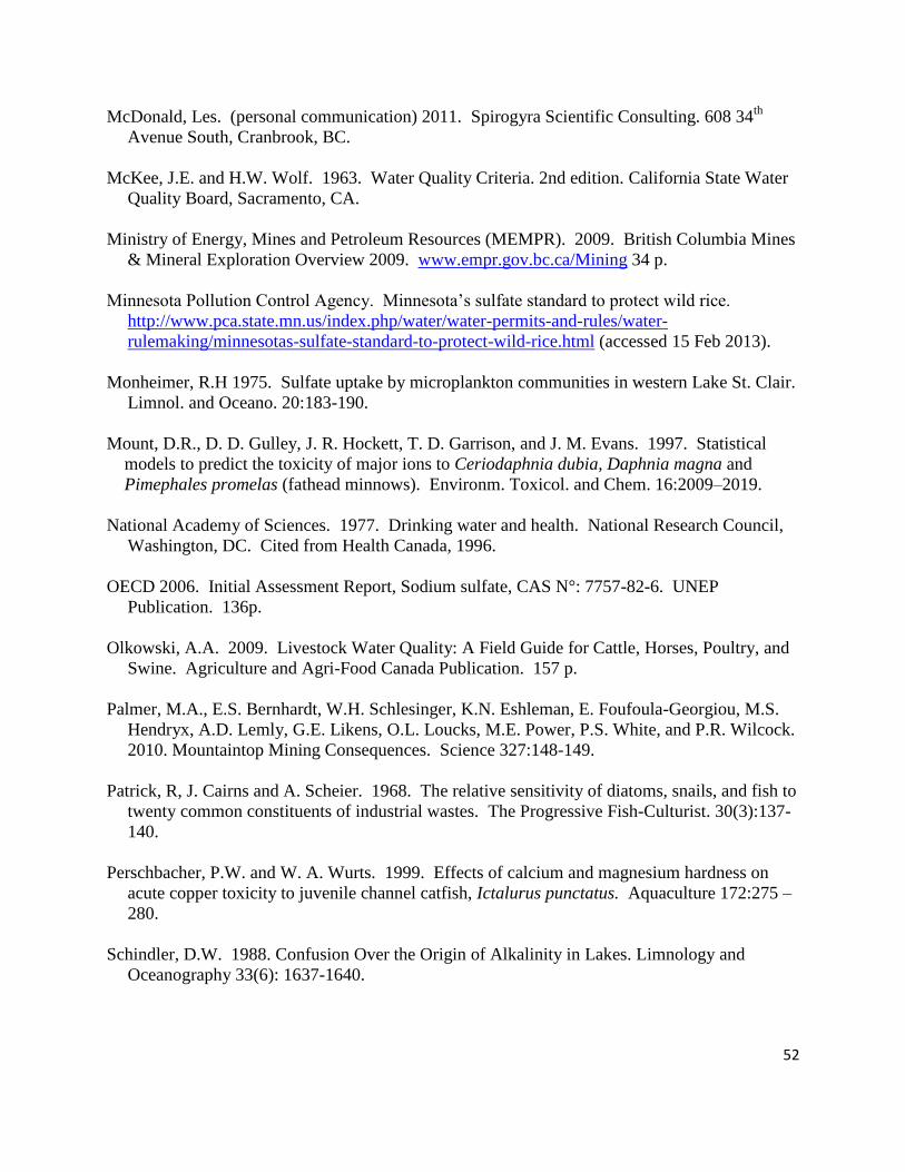
52

McDonald, Les. (personal communication) 2011. Spirogyra Scientific Consulting. 608 34th

Avenue South, Cranbrook, BC.

McKee, J.E. and H.W. Wolf. 1963. Water Quality Criteria. 2nd edition. California State Water

Quality Board, Sacramento, CA.

Ministry of Energy, Mines and Petroleum Resources (MEMPR). 2009. British Columbia Mines

& Mineral Exploration Overview 2009. www.empr.gov.bc.ca/Mining 34 p.

Minnesota Pollution Control Agency. Minnesota’s sulfate standard to protect wild rice.

http://www.pca.state.mn.us/index.php/water/water-permits-and-rules/water-

rulemaking/minnesotas-sulfate-standard-to-protect-wild-rice.html (accessed 15 Feb 2013).

Monheimer, R.H 1975. Sulfate uptake by microplankton communities in western Lake St. Clair.

Limnol. and Oceano. 20:183-190.

Mount, D.R., D. D. Gulley, J. R. Hockett, T. D. Garrison, and J. M. Evans. 1997. Statistical

models to predict the toxicity of major ions to Ceriodaphnia dubia, Daphnia magna and

Pimephales promelas (fathead minnows). Environm. Toxicol. and Chem. 16:2009–2019.

National Academy of Sciences. 1977. Drinking water and health. National Research Council,

Washington, DC. Cited from Health Canada, 1996.

OECD 2006. Initial Assessment Report, Sodium sulfate, CAS N°: 7757-82-6. UNEP

Publication. 136p.

Olkowski, A.A. 2009. Livestock Water Quality: A Field Guide for Cattle, Horses, Poultry, and

Swine. Agriculture and Agri-Food Canada Publication. 157 p.

Palmer, M.A., E.S. Bernhardt, W.H. Schlesinger, K.N. Eshleman, E. Foufoula-Georgiou, M.S.

Hendryx, A.D. Lemly, G.E. Likens, O.L. Loucks, M.E. Power, P.S. White, and P.R. Wilcock.

2010. Mountaintop Mining Consequences. Science 327:148-149.

Patrick, R, J. Cairns and A. Scheier. 1968. The relative sensitivity of diatoms, snails, and fish to

twenty common constituents of industrial wastes. The Progressive Fish-Culturist. 30(3):137-

140.

Perschbacher, P.W. and W. A. Wurts. 1999. Effects of calcium and magnesium hardness on

acute copper toxicity to juvenile channel catfish, Ictalurus punctatus. Aquaculture 172:275 –

280.

Schindler, D.W. 1988. Confusion Over the Origin of Alkalinity in Lakes. Limnology and

Oceanography 33(6): 1637-1640.

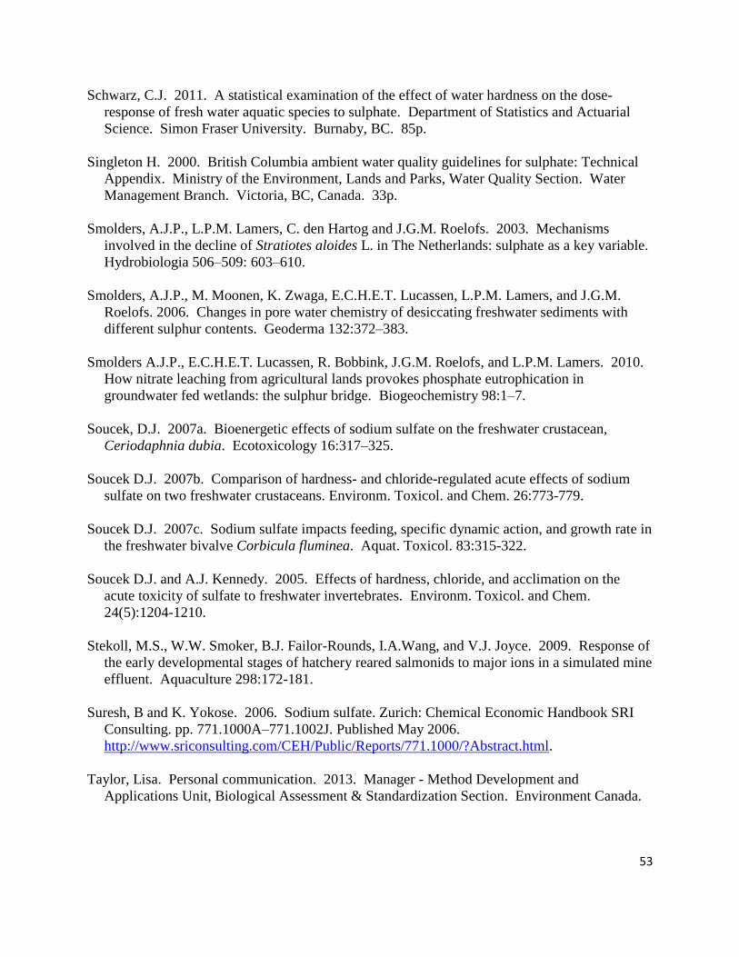
53

Schwarz, C.J. 2011. A statistical examination of the effect of water hardness on the dose-

response of fresh water aquatic species to sulphate. Department of Statistics and Actuarial

Science. Simon Fraser University. Burnaby, BC. 85p.

Singleton H. 2000. British Columbia ambient water quality guidelines for sulphate: Technical

Appendix. Ministry of the Environment, Lands and Parks, Water Quality Section. Water

Management Branch. Victoria, BC, Canada. 33p.

Smolders, A.J.P., L.P.M. Lamers, C. den Hartog and J.G.M. Roelofs. 2003. Mechanisms

involved in the decline of Stratiotes aloides L. in The Netherlands: sulphate as a key variable.

Hydrobiologia 506–509: 603–610.

Smolders, A.J.P., M. Moonen, K. Zwaga, E.C.H.E.T. Lucassen, L.P.M. Lamers, and J.G.M.

Roelofs. 2006. Changes in pore water chemistry of desiccating freshwater sediments with

different sulphur contents. Geoderma 132:372–383.

Smolders A.J.P., E.C.H.E.T. Lucassen, R. Bobbink, J.G.M. Roelofs, and L.P.M. Lamers. 2010.

How nitrate leaching from agricultural lands provokes phosphate eutrophication in

groundwater fed wetlands: the sulphur bridge. Biogeochemistry 98:1–7.

Soucek, D.J. 2007a. Bioenergetic effects of sodium sulfate on the freshwater crustacean,

Ceriodaphnia dubia. Ecotoxicology 16:317–325.

Soucek D.J. 2007b. Comparison of hardness- and chloride-regulated acute effects of sodium

sulfate on two freshwater crustaceans. Environm. Toxicol. and Chem. 26:773-779.

Soucek D.J. 2007c. Sodium sulfate impacts feeding, specific dynamic action, and growth rate in

the freshwater bivalve Corbicula fluminea. Aquat. Toxicol. 83:315-322.

Soucek D.J. and A.J. Kennedy. 2005. Effects of hardness, chloride, and acclimation on the

acute toxicity of sulfate to freshwater invertebrates. Environm. Toxicol. and Chem.

24(5):1204-1210.

Stekoll, M.S., W.W. Smoker, B.J. Failor-Rounds, I.A.Wang, and V.J. Joyce. 2009. Response of

the early developmental stages of hatchery reared salmonids to major ions in a simulated mine

effluent. Aquaculture 298:172-181.

Suresh, B and K. Yokose. 2006. Sodium sulfate. Zurich: Chemical Economic Handbook SRI

Consulting. pp. 771.1000A–771.1002J. Published May 2006.

http://www.sriconsulting.com/CEH/Public/Reports/771.1000/?Abstract.html.

Taylor, Lisa. Personal communication. 2013. Manager - Method Development and

Applications Unit, Biological Assessment & Standardization Section. Environment Canada.

54

Tokuz, R.Y. and W.W. Eckenfelder. 1979. The effect of inorganic salts on the activated sludge

process performance. Water Res. 13(1):99-104.

Tokuz, R.Y. 1986. The effect of high salinity on activated sludge effluent quality. Curr. Pract.

Environ. Sci. Eng. 2:143-154.

Trama, F.B. 1954. The acute toxicity of some common salts of sodium potassium and calcium

to the common Bluegill. (Lepomis macrochirus Rafinesque). Proc. Acad. Nat. Sci.

Philadelphia. 106: 185-205.

US EPA. 1985. National primary drinking water regulations: synthetic organic chemicals,

inorganic chemicals, and microorganisms; proposed rule. Fed. Regist. 50(219): 46936. Cited

from Health Canada, 1996.

US EPA. 1999. Health Effects from Exposure to High Levels of Sulfate in Drinking Water

Study. Office of Water. Center for Disease Control and Prevention. EPA 815-R-99-001, 25

pp.

US EPA. 2003. Drinking Water Advisory: Consumer acceptability advice and health effects

analysis on sulfate. Office of Water (4304T) Health and Ecological Criteria Division,

Washington DC 20460. EPA 822-R-03-007. 29p

US EPA. 2011. http://water.epa.gov/drink/contaminants/unregulated/sulfate.cfm (accessed 22

Feb 2011).

van Dam R.A., A.C. Hogan, C.D. McCullough, M.A. Houston, C.L. Humphrey, and A.J.

Harford. 2010. Aquatic toxicity of magnesium sulfate, and the influence of calcium, in very

low ionic concentration water. Environ. Toxicol. Chem. 29:410–421.

Van der Welle, M.E.W., A.J.P. Smolders, H.J.M. Op den Camp, J.G.M. Roelofs and L.P.M.

Lamers. 2007. Biogeochemical interactions between iron and sulphate in freshwater

wetlands and their implications for interspecific competition between aquatic macrophytes.

Freshwater Biol. 52:434–447.

Welsh, P.G., J. Lipton, G.A. Chapman, and T.L. Podrabsky. 2000a. Relative importance of

calcium and magnesium in hardness-based modification of copper toxicity. Environm.

Toxicol. and Chem. 19:1624–1631.

Welsh, P.G., J. Lipton, and G.A. Chapman. 2000b. Evaluation of water-effect ratio

methodology for establishing site-specific water quality criteria. Environm. Toxicol. and

Chem. 19:1616-1623.

Zak, D., A. Kleeberg and M. Hupfer. 2006. Sulphate-mediated phosphorus mobilization in

riverine sediments at increasing sulphate concentration, River Spree, NE Germany.

Biogeochem. 80:109–119.

55

Zoeteman, B.C.J. 1980. Sensory Assessment of Water Quality. Pergamon Press, New York.

Cited from Health Canada, 1996.