Altitudinal patterns of moth diversity in tropical and subtropical australian rainforests onlinelibr

Altitudinal patterns of moth diversity in tropical andsubtropical Australian rainforests

L. A. ASHTON,1,2* E. H. ODELL,1 C. J. BURWELL,3 S. C. MAUNSELL,1

A. NAKAMURA,4 W. J. F. MCDONALD5 AND R. L. KITCHING1

1Environmental Futures Research Institute and Griffith School of Environment, Griffith University,Nathan, Queensland 4111, Australia (Email: [email protected]), 2Life Sciences Department,Natural History Museum, London, UK, 3Natural Environments Program, Queensland Museum, SouthBrisbane, Australia, 4Key Laboratory of Tropical Forest Ecology, Xishuangbanna Tropical BotanicalGarden, Chinese Academy of Sciences, Yunnan, China; and 5Department of Environment and ResourceManagement, Queensland Herbarium, Biodiversity and Ecosystem Sciences, Toowong, Australia

Abstract Altitudinal gradients are an excellent study tool to help understand the mechanisms shaping commu-nity assembly. We established a series of altitudinal gradients along the east coast of Australia to describe how thedistribution of a hyper-diverse herbivore group (night-flying Lepidoptera) changes across an environmental gra-dient in subtropical and tropical rainforests.Two transects were in subtropical rainforest in the same bioregion, onein south-east Queensland (28.7°S) and one in north east New SouthWales (29.7°S).Two were in tropical rainforest,one in mid-east Queensland (21.1°S) and one in the Wet Tropics of northern Queensland (17.5°S). Replicate plotswere established in altitudinal bands separated by 200 m. Canopy and understorey moths were sampled at thebeginning and end of the wet season using automatic Pennsylvania light traps. We sorted a total of 93 400individuals, belonging to 3035 species.The two subtropical transects in the same region showed similar patterns ofturnover across altitude, with the most distinctive assemblage occurring at the highest altitude. Moth assemblagesin the tropical transects tended to show distinct ‘lowland’ and ‘upland’ communities. For species that were commonacross several of the transects, many were found at lower altitudes in the subtropics and higher altitudes in thetropics, suggesting they are sensitive to environmental conditions, and track their physiological envelopes acrosslatitudes.These results suggest ubiquitous altitudinal stratification in tropical and subtropical Australian rainforests.The marked response of species to latitude and altitude demonstrates they are sensitive to climatic variables and canbe used as indicators to understand future community responses to climate change.

Key words: altitude, beta diversity, climate change, elevation, latitude, tropical and subtropical rainforest.

INTRODUCTION

Altitudinal gradients are excellent study systems forecology, encompassing steep shifts in biotic and abioticfactors in a small geographic area (Hodkinson 2005).They have been used to study the driving forces andmechanisms that underlie patterns in diversity andcommunity structure (Gagne 1979; Hebert 1980;Bravo et al. 2008). Mountain ecosystems andaltitudinal gradients are notable for their high level ofdiversity (Körner 2000) and have become an impor-tant tool for investigating the factors that shape thedistributions of organisms, for observing shifts inaltitudinal ranges and for predicting future responsesto climate change (Shoo et al. 2006; Fischer et al.2011).

Organisms may exhibit altitudinal stratification, withsome species occupying very small altitudinal ranges,leading to a high turnover in assemblage structureacross altitudes. On the other hand, species that areable to cope with a wide range of environmental con-ditions may occur across an entire altitudinal gradient.Generally, studies have found altitudinal stratificationin assemblages, including in ants (Burwell &Nakamura 2011), moths (Brehm & Fiedler 2003;Ashton et al. 2011), beetles (Escobar et al. 2005),collembola (Maunsell et al. 2012), birds (Williamset al. 2010), mammals (Williams 1997) and vegetation(Hemp 2006). Different taxonomic groups mayrespond in distinctive ways to altitude (Stork &Brendell 1990). Many species may be restricted toonly high altitudes and are often associated withhigh levels of endemism (Kessler 2002; Szumik et al.2012).

The relationship between species richness and alti-tude can be variable. The two most commonly

*Corresponding author.Accepted for publication July 2015.

Austral Ecology (2015) ••, ••–••

bs_bs_banner

© 2015 Ecological Society of Australia doi:10.1111/aec.12309

observed patterns are linear declines in richness withincreasing altitude (Hebert 1980), or unimodal(humped) shaped patterns in species richness (Beck &Chey 2008). Several factors may influence observedspecies patterns, including the altitudinal range of thestudied gradient which often reflects the degree ofdisturbance in lowland areas due to human impact(these disturbed areas are usually avoided byresearchers). In such cases, it is not possible to incor-porate the full altitudinal range within an ecosystem,and sampling points have to be placed in locationswhere intact forest is available.The scale or resolutionat which altitudinal studies are conducted (i.e. thedistance between altitudinal bands) may also impactobserved patterns, and can, in fact, produce com-pletely different patterns of species richness (humpshaped or linear) (Rahbek 2005; Nogués-Bravo et al.2008).

Climate change is driving a range of responses inspecies, communities and ecosystems (Steffen et al.2009) and is predicted to lead to a variety of severeimpacts including species extinction, range contrac-tion and mismatched phenologies of interactingspecies (Hughes 2000; Williams et al. 2003). Distribu-tion shifts are predicted for terrestrial biota(Sekercioglu et al. 2008; Kreyling et al. 2010;Laurance et al. 2011). Such shifts may occur whenspecies climatic envelopes (the limits of individualspecies tolerances of environmental variables such asprecipitation and temperature) move as a result ofchanged environmental conditions (Kullman 2001;Walther et al. 2002; Battisti et al. 2006).

Tropical species may be particularity vulnerableto climate-driven distribution shifts, as they tend toexhibit low ranges of thermal tolerance, linked towarmer, more seasonally stable environments(Laurance et al. 2011; Cadena et al. 2012). High alti-tude species are also particularly at risk and may showearly signs of climate driven responses (Dirnbock et al.2011). Another sensitive area to monitor is the ecotonebetween cloud forest and lower altitude forest, asclimate change-driven drying may also produce earlyclimate change responses (Foster 2001). Althoughchanges to rainfall under future climate change sce-narios are hard to predict (Reisinger et al. 2014), theaverage level of the cloud base is predicted to rise,which is particularly important for rainforest in the dryseason where cloud stripping maintains high moisturelevels (Still et al. 1999). An average temperatureincrease of 4°C by 2100 (a scenario that is perceived asbeing increasingly likely (Sanford et al. 2014) wouldresult in an 800 m upward altitudinal shift in climaticconditions (Malhi & Phillips 2004). More optimisticclimate change scenarios still predict upwards shifts of450 m (Loope & Giambelluca 1998).

Australian biota are predicted to display significantrange shifts, population declines and contraction, and

extinctions, especially in areas with large numbers ofregionally endemic species such as the tropical rain-forests of the Wet Tropics. In Australia, there are fewdata on the impacts of climate change on the biota,especially invertebrates (but see Beaumont andHughes (2002)). In order to understand how speciesare responding to climate change, we need to generatebaseline data on the current distributions of species.By examining species distributed across tropical andsubtropical rainforests in Australia and investigatinghow their altitudinal ranges are driven by environmen-tal variables at different latitudes, we will be better ableto predict how these species may respond to furtherclimate warming.

We sampled moths along altitudinal transects inBorder Ranges (BR) and Lamington (LAM)National Parks, which are within the same bioregion,in order to compare assemblages essentially drawnfrom the same regional species pool but influencedby key environmental differences, principally, in thiscase, aspect. Aspect is an important factor determin-ing the structure of plant communities, and by exten-sion, their insect herbivores. It is particularlyimportant for the subtropical rainforests of NewSouth Wales (NSW) and south-east Queensland,especially in winter, where a south facing slope mayreceive less than 10 h of sunlight in a day (Laidlawet al. 2011). The importance of aspect is reduced intropical rainforests closer to the equator, where southand north facing slopes receive similar amounts ofdaily sunlight. Consequently, the comparison of thesesubtropical transects should provide insight into theinfluence of local environmental conditions on mothassemblages.

Tropical rainforest may present a different suite ofenvironmental drivers compared to subtropical forests.Accordingly, we established altitudinal transects at dif-ferent tropical latitudes in Queensland to assess pat-terns of altitudinal stratification in locations withdifferent climates, weather patterns and biogeographi-cal histories. Here, we investigate whether tropicalrainforest moths respond to changes in environmentalconditions across altitudes in a similar way to subtropi-cal assemblages. Tropical species may be less able tocope with a wide range of temperature fluctuations(Janzen 1967; Addo-Bediako et al. 2000; Tewksburyet al. 2008). We therefore hypothesize that thealtitudinal stratification of moth assemblages in tropi-cal areas will show strong turnover across altitudinalzones, as environmental factors that shift with altitudemay be a major constraining factor on the distributionsof individual species. This is the first study of a keyinsect herbivore group across multiple altitudinal gra-dients in Australia. It demonstrates the insights thatcan be gained from spatially replicated studies acrosssubstantial geographical distances using standardizedsampling methodologies.

2 L. A. ASHTON ET AL.

© 2015 Ecological Society of Australiadoi:10.1111/aec.12309

METHODS

At each of four locations (Fig. 1), we established analtitudinal transect, with four 20 × 20 m replicate plotswithin five or six altitudinal bands, separated by approxi-mately 200 m of altitude. Within-band plots were placed atleast 400 m apart and cool drainage areas associated withstream lines were avoided, however, at some locations thiswas not possible. At each plot, all woody stems with a diam-eter at breast height (dbh) greater than 5 cm were tagged andmeasured.

Lamington and Border Ranges National Parks

Lamington and BR National Parks are within the GondwanaRainforests of Australia World Heritage Area, which containsone of the largest remaining areas of undisturbed subtropicalrainforest in the world.The Investigating Biodiversity of Soiland Canopy Arthropods (IBISCA) Queensland Project,within which the moth data presented here were collected,was conducted in Lamington NP (latitude 28°1′S) between2006 and 2010 (Ashton et al. 2011; Kitching et al. 2011).Four replicate plots were located within each of fiveelevational bands at 300, 500, 700, 900 and 1100 m a.s.l.Weaimed to study assemblages across continuous rainforestgradients. The highest available altitude at Lamington is1100 m a.s.l. and below 300 m much of the forest has beencleared with only remnant patches remaining.The vegetationacross this transect is complex notophyll vine forest at the300 m–900 m a.s.l. plots, and simple notophyll fern forest atthe 1100 m a.s.l. plots, dominated Nothofagus moorei (Ant-arctic Beech) (Laidlaw et al. 2011). Where possible, plotswere located on soils derived from Cainozoic igneous rock,

with a north-easterly aspect (Strong et al. 2011).This regionis subject to strong seasonality, with pronounced wet and dryseasons (Morand 1996). The base of the cloud cap sitsbetween 800 m and 900 m a.s.l., which can provide 40% oftotal annual precipitation (Hutley et al. 1997).

Border Ranges National Park (latitude 28.2′°S), covers318 km2 and was logged between 1965 and 1975. Averageannual rainfall in the region is 2500–4000 mm, and soils arekraznozems or ferrosols (Isbell 2002). As at Lamington, thebase of the cloud cap sits between 800 m and 900 m a.s.l.,and regulates moisture above this level. There is approxi-mately 20 km of continuous subtropical rainforest betweenthe Border Ranges and Lamington transects. At BorderRanges, the altitudinal extent is lower than at Lamington,therefore, four replicate plots were located at 300, 500, 700,900 and 1010 m a.s.l. Border Ranges was slightly cooler thanLamington (see Appendix S1 for a description of tempera-ture data collected during this study).

Eungella National Park (EU)

Eungella (EU) National Park is located approximately halfway between the Wet Tropics of north Queensland and thesubtropical rainforests of south-east Queensland (latitude21°S). Some of the forest in this region has been subject tologging, mining and clearing for dairy farming. In 1941, theNational Park was established and now conserves 300 km2 ofrainforest on primarily granitic soils (Graham 2006). Fourreplicate plots were located at 200, 400, 600, 800, 1000 and1200 m a.s.l., encompassing the available altitudinal heightat Mt. Dalrymple, Mt. Henry and Mt. William, down to200 m a.s.l., below which most forest has been cleared. Wecollected soil samples and measured temperature usingi-Buttons between 01.12.14 and 01.03.15. Mean tempera-tures decreased by 0.6°C per 100 m increase in altitude.

Mt. Lewis National Park

The AustralianWetTropicsWorld Heritage Area is the largestarea of rainforest in Australia, covering 2 million hectares, ina series of fragmented patches. Mt. Lewis (ML) NationalPark (latitude 16.3°S) is located 80 km north-north-west ofCairns, and protects areas of both primary and loggedupland rainforest, encompassing a total area of 229 km2.Four replicate plots were located at 400, 600, 800, 1000 and1200 m a.s.l. (the highest altitudinal extent at ML). Rainfalland temperature data were collected by researchers at JamesCook University.Temperature data were collected at one plotper altitude between 01.01.2006 and 09.12.2008. Meantemperatures ranged between 21°C at 400 m a.s.l. to 16°C at1200 m a.s.l., an average decrease of 0.5°C per 100 m. Dailyrainfall data between 01.01.2006 and 01.01.2009 were col-lated from data from the Bureau of Meteorology’s AustralianWater Availability Project (http://www.bom.gov.au/jsp/awap/rain/index.jsp). Average annual rainfall ranged between2140 mm at 400 m a.s.l. and 2924 mm at 1200 m a.s.l.

Sampling and light traps

Each altitudinal transect was sampled at the beginning andend of the wet season. Lamington was sampled from 14–30

Fig. 1. Map of altitudinal gradient locations – BorderRanges National Park, northern Nsw, Lamington NationalPark, south-east Qld, Eungella National Park, Qld and Mt.Lewis National Park north Qld.

MOTH DIVERSITY ACROSS ALTITUDE AND LATITUDE 3


October 2006 and 10 March–2 April 2007, as part of theIBISCA–Queensland project. Due to time constraints, two300 m a.s.l. plots were not sampled in October 2006, andtwo 500 m a.s.l. plots were not sampled in March/April2008. Border Ranges was sampled from 4–22 April 2011 and27 October–12 November 2010, Mt. Lewis from 21November–13 December 2009 and 1–18 April 2011, andEungella from 4–30 November 2013 and 16 March–12 April2014.

Moths were sampled using Pennsylvania light traps (Frost1957), employing an 8-watt actinic UV bulb and run forthree nights from dusk to dawn.We sampled both the canopyand understorey fauna, to account for vertical stratification(Schulze et al. 2001; Brehm 2007) and, therefore, get a betterpicture of the overall forest moth fauna (Beck et al. 2002).Understorey traps were situated approximately 2 m abovethe ground while those in the canopy were suspended in theupper half of the canopy approximately 20 to 35 m above theground depending on the height of the forest. Canopy trapswere located where canopy lines could be shot using a com-pound bow, understorey traps were placed within 10 m of thecanopy lines. All moths with a forewing length greater than1 cm and, in addition, all Pyraloidea (i.e. Crambidae andPyralidae), were processed.

Analysis

Data from three nights of collection in the canopy and under-story at each plot were pooled, and data collected at thebeginning and end of the wet season were combined.We logtransformed the data prior to multivariate analysis to over-come the influence of dominant species (Southwood &Henderson 2000). We constructed plot-based similaritymatrices for each transect (LAM, BR, EU, ML) using theBray–Curtis similarity measure (Bray and Curtis 1957).From these matrices non-metric multidimensional scalingwas conducted, set to 1000 random starts, to produceordination plots illustrating the relationships among assem-blages of the plots. Using the same similarity matrices,we performed ‘permutation-based analysis of variance’(PERMANOVA) (Anderson et al. 2008) using 1000 permu-tations to test for differences between a priori groups (i.e.adjacent altitudinal zones). Another plot-based Bray–Curtissimilarity matrix for each transect (LAM, BR, EU, ML), wascreated, based on tree (dbh > 5 cm) assemblage data and aMantel Test of correlation between the moth and tree assem-blages performed using Spearman’s rank correlation and1000 permutations.

For each altitudinal transect, we used a distance-basedlinear model (DistLM) (Ardle & Anderson 2001) to identifyplot-based environmental variables (biotic and abiotic) thatwere significantly correlated with moth assemblage structure.Across all transects, analysis incorporated data on altitude,tree species richness, air temperature (average, minimum andmaximum). At Lamington, we also measured soil properties(moisture, pH, total organic content, potassium and carbon)and inferred fog events. At Eungella, we collected soil vari-ables (sodium, nitrogen, calcium, clay and total organiccontent). The Mt. Lewis analysis incorporated rainfall, soiltemperature, carbon, nitrogen and potassium. Many of thesevariables were highly correlated; the BEST procedure was

used to run sequential tests to determine the combination ofvariables that had the best explanatory power (r2). Significantvariables (P < 0.05) were superimposed onto moth assem-blage ordination plots.

As moth samples can be highly variable, and some siteswere under-sampled, estimated moth richness is a moreinformative metric than observed species richness.We there-fore present the total estimated species richness at each alti-tude which was estimated using sample-based rarefactioncurves in EstimateS (Colwell 2013). We used the non-parametric Chao1 estimator, as this has been suggested formobile organisms (Brose et al. 2003).We plotted the pairwiseBray–Curtis similarity of moth assemblages between plotsagainst the altitudinal distance between plots in order toillustrate how the relationship between beta-turnover shiftsacross altitude. We also set out to establish indicator specieswhich are altitudinally restricted in order to allow possiblere-sampling in the future to monitor any climate change-driven shifts in altitudinal distributions.The indicator speciespresented here are those that are indicative of a singlealtitudinal band or of two or three altitudinal bands (e.g.found at 700 m, 900 m and 1100 m a.s.l.). IndVal (version2.1; Dufrêne & Legendre 1997) analysis was conducted onall species represented by more than 35 individuals from atransect, as rare species are unlikely to be useful indicatorspecies.This analysis was conducted in the R statistical envi-ronment (R Development Core Team 2010), using theIndVal procedure in the labdsv package (Roberts 2010).Thismethod uses a randomization procedure to identify taxa thatare indicative of a priori groups (i.e. altitudes). Based on thespecificity (proportion of replicate plots, within groups, occu-pied by the species) and fidelity (proportion of the specieswithin a group, across all replicates) of the species within agroup, indicator values are calculated as a percentage. Weselected species with an indicator value greater than 70%.Once this analysis had established statistically significantindictor species, those which were hard to identify, or had notyet been assigned a scientific name were removed from thefinal set of indicator species.

For the purposes of this paper,we only present those speciesthat occurred across two or more of the four altitudinalgradients, as we were primarily interested in the altitudinaldistribution of species at different latitudes. We also collateddistributional data, which included altitude information, forthe indicator species from specimens in the collections of theQueensland Museum, Brisbane, the Australian NationalInsect Collection, Canberra and the Australian Museum,Sydney. Although these specimen data do not encompass theentire ranges of these species, they provide some indication ofthe wider latitudinal and altitudinal distributions of the indi-cator species.We also note that a detailed analysis of canopy/understorey contrasts in moth assemblage composition will bethe subject of a separate contribution.

RESULTS

Border Ranges National Park

Border Ranges sampling (November and April 2010)produced a total of 40 859 individuals belonging to



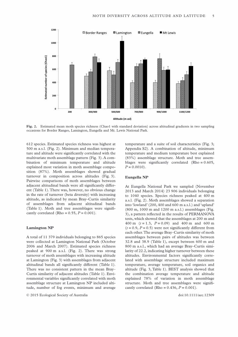
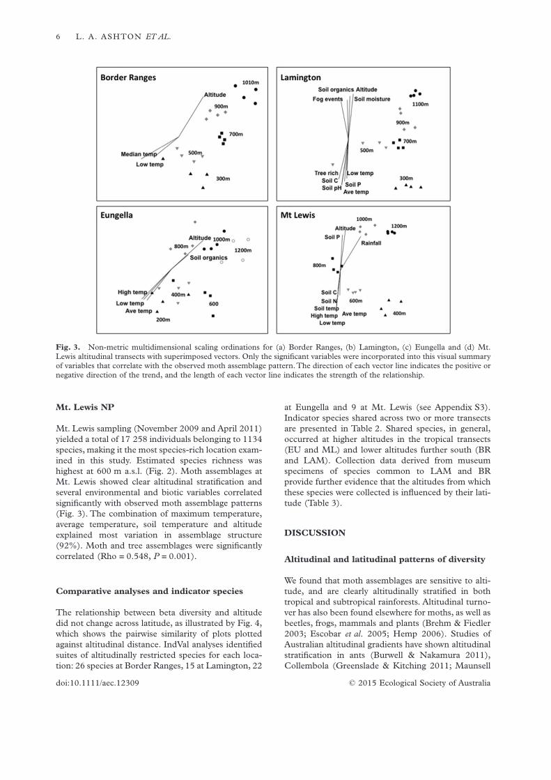
612 species. Estimated species richness was highest at500 m a.s.l. (Fig. 2). Minimum and median tempera-ture and altitude were significantly correlated with themultivariate moth assemblage pattern (Fig. 3). A com-bination of minimum temperature and altitudeexplained most variation in moth assemblage compo-sition (87%). Moth assemblages showed gradualturnover in composition across altitudes (Fig. 3).Pairwise comparisons of moth assemblages betweenadjacent altitudinal bands were all significantly differ-ent (Table 1). There was, however, no obvious changein the rate of turnover (beta diversity) with increasingaltitude, as indicated by mean Bray–Curtis similarityof assemblages from adjacent altitudinal bands(Table 1). Moth and tree assemblages were signifi-cantly correlated (Rho = 0.55, P = 0.001).

Lamington NP

A total of 11 379 individuals belonging to 865 specieswere collected at Lamington National Park (October2006 and March 2007). Estimated species richnesspeaked at 900 m a.s.l. (Fig. 2). There was strongturnover of moth assemblages with increasing altitudeat Lamington (Fig. 3) with assemblages from adjacentaltitudinal bands all significantly different (Table 1).There was no consistent pattern in the mean Bray–Curtis similarity of adjacent altitudes (Table 1). Envi-ronmental variables significantly correlated with mothassemblage structure at Lamington NP included alti-tude, number of fog events, minimum and average

temperature and a suite of soil characteristics (Fig. 3;Appendix S2). A combination of altitude, minimumtemperature and medium temperature best explained(83%) assemblage structure. Moth and tree assem-blages were significantly correlated (Rho = 0.605,P = 0.0010).

Eungella NP

At Eungella National Park we sampled (November2013 and March 2014) 23 906 individuals belongingto 1040 species. Species richness peaked at 400 ma.s.l. (Fig. 2). Moth assemblages showed a separationinto ‘lowland’ (200, 400 and 600 m a.s.l.) and ‘upland’(800 m, 1000 m and 1200 m a.s.l.) assemblages (Fig.3), a pattern reflected in the results of PERMANOVAtests, which showed that the assemblages at 200 m and400 m (t = 1.3, P = 0.09) and 400 m and 600 m(t = 0.9, P = 0.5) were not significantly different fromeach other.The average Bray–Curtis similarity of mothassemblages between pairs of altitudes was between32.8 and 38.9 (Table 1), except between 600 m and800 m a.s.l., which had an average Bray–Curtis simi-larity of 22.2, indicating higher turnover between thesealtitudes. Environmental factors significantly corre-lated with assemblage structure included maximumtemperature, average temperature, soil organics andaltitude (Fig. 3, Table 1). BEST analysis showed thatthe combination average temperature and altitudeexplained 78% of variation in moth assemblagestructure. Moth and tree assemblages were signifi-cantly correlated (Rho = 0.436, P = 0.001).

Fig. 2. Estimated mean moth species richness (Chao1 with standard deviation) across altitudinal gradients in two samplingoccasions for Border Ranges, Lamington, Eungella and Mt. Lewis National Park.



Mt. Lewis NP

Mt. Lewis sampling (November 2009 and April 2011)yielded a total of 17 258 individuals belonging to 1134species, making it the most species-rich location exam-ined in this study. Estimated species richness washighest at 600 m a.s.l. (Fig. 2). Moth assemblages atMt. Lewis showed clear altitudinal stratification andseveral environmental and biotic variables correlatedsignificantly with observed moth assemblage patterns(Fig. 3). The combination of maximum temperature,average temperature, soil temperature and altitudeexplained most variation in assemblage structure(92%). Moth and tree assemblages were significantlycorrelated (Rho = 0.548, P = 0.001).

Comparative analyses and indicator species

The relationship between beta diversity and altitudedid not change across latitude, as illustrated by Fig. 4,which shows the pairwise similarity of plots plottedagainst altitudinal distance. IndVal analyses identifiedsuites of altitudinally restricted species for each loca-tion: 26 species at Border Ranges, 15 at Lamington, 22

at Eungella and 9 at Mt. Lewis (see Appendix S3).Indicator species shared across two or more transectsare presented in Table 2. Shared species, in general,occurred at higher altitudes in the tropical transects(EU and ML) and lower altitudes further south (BRand LAM). Collection data derived from museumspecimens of species common to LAM and BRprovide further evidence that the altitudes from whichthese species were collected is influenced by their lati-tude (Table 3).

DISCUSSION

Altitudinal and latitudinal patterns of diversity

We found that moth assemblages are sensitive to alti-tude, and are clearly altitudinally stratified in bothtropical and subtropical rainforests. Altitudinal turno-ver has also been found elsewhere for moths, as well asbeetles, frogs, mammals and plants (Brehm & Fiedler2003; Escobar et al. 2005; Hemp 2006). Studies ofAustralian altitudinal gradients have shown altitudinalstratification in ants (Burwell & Nakamura 2011),Collembola (Greenslade & Kitching 2011; Maunsell

Fig. 3. Non-metric multidimensional scaling ordinations for (a) Border Ranges, (b) Lamington, (c) Eungella and (d) Mt.Lewis altitudinal transects with superimposed vectors. Only the significant variables were incorporated into this visual summaryof variables that correlate with the observed moth assemblage pattern.The direction of each vector line indicates the positive ornegative direction of the trend, and the length of each vector line indicates the strength of the relationship.



et al. 2012) and birds (E. Leach. pers. comm.). Thealtitudinally stratified moth assemblages at all fourlocations suggest that altitude (or some associated cor-relate) is important in structuring moth communities.As the vegetation assemblage structure also exhibitedaltitudinal turnover, and was significantly correlatedwith moth assemblages, it is difficult to untangle therelative importance of these abiotic and biotic drivers.We hypothesized that moth species in the tropicswould be more sensitive to altitude than those in thesubtropics; however, the rate of turnover did not shiftwith decreasing latitude. If tropical species were morealtitudinally restricted, we would expect the beta-diversity turnover across altitudinal distance to besteeper in the tropical locations, and perhaps, morealtitudinally restricted indicator species. What wefound was a uniform relationship between beta-turnover and altitude across tropical and subtropicalgradients and few altitudinally restricted indicatorspecies in the tropical locations.

There was strong altitudinal turnover in mothassemblages in both subtropical and tropical transects

but with some key differences. In the subtropical loca-tions, we found stepwise turnover in assemblage com-position and a unique moth assemblage at 1100 ma.s.l. associated with a change in the vegetation fromcomplex notophyll vine forest to simple microphyllfern forest with a monodominant canopy of Nothofagusmoorei. In the tropical transects, however, there wasgreater turnover at mid-altitudes separating mothassemblages into lowland and upland faunas. In theWet Tropics, within which our Mt. Lewis transect islocated, a similar division is found in vertebrate assem-blages, including mammals (Williams 1997) and birds(Williams et al. 2010). These observed differences inturnover between tropical and subtropical transectsare also apparent in the vegetation assemblages andmay be largely driven by the warmer, wetter conditionsin the tropics, influencing the height of the cloud capand the stability of moisture through time. The sub-tropical higher altitudinal sites may exhibit more fre-quent drying, producing a gradual turnover inassemblage structure across altitude, driven primarilyby the altitudinal shifting of environmental variablesrather than by the presence of the cloud cap.

Although fewer species were collected from BorderRanges (612 spp.) than Lamington (865 spp.), bothtransects displayed stepwise turnover in moth assem-blages with increasing altitude, thus their differingaspects did not dramatically influence the pattern ofaltitudinal stratification. We recorded a lower averagetemperature gradient at Border Ranges compared withLamington, which may be due to microhabitat effects,different aspects or to high rainfall levels that occurredduring the year temperature was recorded at BorderRanges. The temperature differences, between theselocations, which are only 20 km apart, may influencethe altitudinal ranges of species. Of the seven indicatorspecies found at both locations, six had a distributionextending one altitudinal band lower at Border RangesNational Park. This suggests that these species areparticularly sensitive to temperature. That the distri-butions of these shared indicator species are driven bytemperature is supported by museum specimen data,which indicate they are generally found at higher alti-tudes at lower latitudes and at lower altitudes at higherlatitudes. For example, Xylodryas leptoxantha, found at900 m and 1100 m a.s.l. at Lamington, and 700 m,900 m and 1100 m a.s.l. at Border Ranges, has beenrecorded as low as 245 m in Coffs Harbour, NSW(30°2 S). Three species collected at Lamington andBorder Ranges, Dyscheralcis crimnodes, Heterochastaconglobate (Geometridae, Larentiinae) and Eurychoriafictilis also occur in warmer tropical forests, but havebeen only recorded at or above 1500 m a.s.l., suggest-ing that these species altitudinal distributions arerestricted by temperature and/or other correlatedfactors that shift with altitude (all species mentionedabove belong to Geometridae, Ennominae unless

Table 1. Metrics of pairwise comparisons between adja-cent altitudinal bands, for Border Ranges, Lamington,Eungella and Mt. Lewis altitudinal gradients; permutationalANOVA results (t and P values), average Bray–Curtis simi-larity, and average distance among multivariate centroids. Allaltitudinal bands at Border Ranges, Lamington and Mt.Lewis are significantly different (P > 0.05). At Eungella,there was no significant difference between 200 and 400 mand 400 and 600 m at Eungella. There was no consistentpattern of increasing or decreasing similarity or distanceamong centroids across altitude

Location Permanova

AverageBray–Curtis

similarity

Border Ranges t P300 and 500 1.301 0.037 50.175500 and 700 2.106 0.031 46.803700 and 900 1.940 0.035 50.589900 and 1100 2.012 0.027 45.949Lamington t P300 and 500 1.801 0.036 25.976500 and 700 1.439 0.026 35.029700 and 900 1.577 0.028 38.236900 and 1100 1.816 0.031 38.31Eungella t P200 and 400 1.319 0.088 37.562400 and 600 0.989 0.512 36.919600 and 800 1.470 0.033 22.248800 and 1000 1.280 0.049 32.7461000 and 1200 1.284 0.032 38.957Mt. Lewis t P400 and 600 1.712 0.033 31.099600 and 800 1.664 0.025 34.075800 and 1000 1.717 0.036 29.3531000 and 1200 1.561 0.030 35.640



Fig. 4. Pairwise Bray–Curtis dissimilarity values of moth assemblages, plotted against the difference in actual altitude at BorderRanges, Lamington, Eungella and Mt. Lewis.

Table 2. Species of moth that are common across at least three of our four altitudinal gradients – Border Ranges, Lamington,Eungella and Mt. Lewis. Generally, species are found at higher altitudes in our tropical transects and lower altitudes furthersouth

Species BR LAM EU ML

Larophylla amimeta 700–1100 900–1100Lyelliana dryophylla 700–1100 900–1100Eurychoria fictilis 700–1100 900–1100Heterochasta conglobata 700–1100 900–1100Dyscheralcis crimnodes 900–1100 700–1100Xylodras leptoxantha 700–1100 900–1100Middletonia hemichroma 900–1100 1100Conogethes punctiferalis 300 400–800Pleuropyta bateata 300 400Orthaga thyrusalis 300 400–600Taxeotis sp. 500–900 600–1000Prorodes mimica 300 400–800 600–1200Taxeotis epigea 500–900 1000 1000Endrotricha mesenterialis 1100 500–1000 1200Agris convolvulii 1100 600–1000Prophanta caletoralis 400–600 400–600Paradromulia ambigua 800–1000 400–800Parotis atlitalis 400–800 600Maruca testulalis 400–600 600–1200Calamidia hirta 800 800Endrotricha dispergens 400 1200



otherwise noted). In addition, indicator species thatoccurred at two or more of our latitudinal locationsgenerally occurred at higher altitudes towards thetropics, likely tracking their physiological envelopes orthat of their host plants.

Altitudinal patterns of diversity

Species richness generally showed a mid-altitude peak,similar to a number of previous altitudinal mothstudies (Brehm et al. 2007; Choi & An 2010).Although there was variation in which particular alti-tude had the highest estimated richness at each loca-tion, it was generally between 400 and 600 m a.s.l.How do alternative explanations help interpretation ofour data from the subtropical and tropical transects?The ‘mid-domain effect’ in which mid-altitude peaksare produced by the random overlap of species occur-rences across altitudes which are postulated to repre-sent homogenous habitats (Colwell & Lees 2000) isfundamentally a neutral explanation. Accordingly,unless host plant distributions form a mid-altitudepeak, this explanation seems weak for mothdistributions. There is, generally, no such peak in theplant data (see Appendix S4). Another explanation isthat mid-altitude peaks are the result of overlapping

ecotones from adjacent ecosystems (e.g. the coinci-dence of the upper bounds of low altitude ecosystemswith the lower bounds of the upper altitudes ecosys-tems (Terborgh 1971)). Finally, species-area effectscould produce a mid-altitude peak when lower alti-tudes have been substantially modified by humanactivities (McCoy 1990), a likely contributor to thepatterns we observe simply because, for all of ourtransects, it was not possible to sample below around300 m a.s.l. as most of the lower forest had beencleared. Our results, based on Australian altitudinaltransects up to 1200 m a.s.l. (the highest availablealtitudinal extents) also may not reach high enoughaltitudes required in order to capture the high-altitudedecline in species richness observed elsewhere(monotonic declines) or the more clearly defined mid-altitudinal peaks observed in some tropical locations.

Altitudinal gradients – indicators ofclimate change

High altitude communities are isolated from othermountain tops and accordingly, have lower rates ofimmigration and higher rates of extinction (Lomolino2001). Mountain ecosystems today represent areas ofhigh conservation concern (Foster 2001), containing

Table 3. Indicator species common between Lamington (LAM)and Border Ranges (BR). In all but one case (Dyscheralciscrimnodes) the indicators at BR are present one altitudinal band below those at LAM. Museum records gathered for these speciesillustrate that indicators are found at higher altitudes in North Queensland and lower altitudes further south in NSW, supportingthe hypothesis that these species distributions are primarily driven by temperature

Name LAM (m a.s.l.) BR (m a.s.l.) Museum records location Lat Ca (S) Altitude (m a.s.l.)

Xylodryasleptoxantha

900, 1100 700, 900, 1100 Bunya Mountains, QLD 26°29 1065 mGibraltar Range, QLD 29°28 950 mAcacia Plateau, NSW 28°19 915 mClyde Mountain, NSW 35°24 730 mCambewarra Mountain NSW 34°46 620 mDorrigo NP, NSW 30°22 520 mMt. Warning, NSW 28°24 500 mUp Allyn R, NSW 32°10 455 mCoffs Harbor 30°15 245 m

Dyscheralciscrimnodes

700, 900, 1100 900, 1100 Bellenden-Ker, north QLD 17°15 1560 mPaluma, QLD 19°1.7 900 m

Heterochastaconglobata

900, 1100 700, 900, 1100 Bellenden-Ker, QLD 19°0.6 1560 m, 1500 mMt. Bartie Frere, QLD 17°23 1500 mClyde Mt., NSW 35°24 731 m

Eurychoria fictilis 900, 1100 700, 900, 1100 Bellenden-Ker, QLD 19°0.6 1560 mMt. Edith, QLD 17°4.5 1035 m

Lyelliana dryophylla 900, 1100 700, 900, 1100 Killarney, NSW 28°18 920 mLarophylla amimeta 900, 1100 700, 900, 1100 New England, NSW 30°29 1585 m

Coneac, NSW 31°51 900 mKillarney, NSW 28°18 920 mCambewarra Mountain, NSW 34°46 620 m

Middletoniahemichroma

1100 900, 1100 Barrington Tops, NSW 31°56 1545 mNew England, NSW 30°29 1615 mSpringbrook, NSW 28°11 700 m



high numbers of endemic, endangered and climatesensitive species, often with small altitudinal ranges(Loope & Giambelluca 1998; Williams et al. 2003).Mountain ecosystems are, by virtue of these features,also sensitive indicator systems, and may be used asearly warning tools for the monitoring of climatechange responses (Beniston et al. 1997). We haveestablished four suites of altitudinally restricted mothindicator species in Australia and demonstrated (forthe shared species) their altitudinal ranges shiftupslope towards the tropics.These insects are suitableclimate indicator species, as our analysis of theirgeneral distributions shows that they are highly sensi-tive to climate. They are easy to identify and readilycollected (Kitching & Ashton 2014). The utility ofthese indicators in the tropics, where there can be largeinter-annual fluctuations in insect populations, mayrequire additional testing. It is also important to notethat there are physical limits to further distributionshifts of species to higher altitudes and latitudes inAustralia, as, in many cases, there are simply no higheraltitudes or latitudes accessible with suitable habitat orhost plants.

Our results show that the altitudinal stratification ofmoths is ubiquitous across different latitudes, foresttypes and biogeographic areas.This research has estab-lished baseline data which can be used to assess futureimpacts of climate change. These data, however,have value beyond simply setting baselines: they haveadded to our knowledge of how a hyper-diverse insectgroup is distributed across environmental gradients –altitudinally and latitudinally. An intrinsic quality ofthis type of extensive baseline research is the novel andcomprehensive faunistic and biogeographical datasetsthat are generated concerning groups of organisms forwhich very little existing information has been avail-able in Australia.

ACKNOWLEDGEMENTS

The field work at Eungella which was conducted aspart of the Eungella Biodiversity Survey was funded bythe Mackay Regional Council and Griffith University.We thank the many community volunteers that madethis project a reality. Lamington National Park datawere collected during the IBISCA-Qld project fundedby the Queensland Department of State Development(a Smart State initiative), Griffith University, Queens-land Museum, Global Canopy Programme, NRM Qldand Queensland National Parks Association. Thisproject was assisted by over 50 volunteers, many ofwhom helped in the collection of moth samples whichwas coordinated by D. Putland. Border Ranges andMt. Lewis field work was assisted by John Gray whovolunteered several months of his time.Thank you alsoto Casey Hall, Christy Harvey and Conservation Vol-

unteers Australia for field work assistance. Botanicalidentification was carried out by Dr W.J.D. McDonald(all locations), Melinda Laidlaw (Lamington), JohnHunter and Stephanie Horton (Border Ranges) andDale Arvidsson (Eungella).

REFERENCES

Addo-Bediako A., Chown S. L. & Gaston K. J. (2000) Thermaltolerance, climatic variability and latitude. Proc. R. Soc.Lond. B 267, 739–45.

Anderson M. J., Gorley R. N. & Clarke K. R. (2008)PERMANOVA+ for PRIMER: Guide to Software and Statis-tical Methods. PRIMER-E, Plymouth.

Ardle B. H. M. & Anderson M. J. (2001) Fitting multivariatemodels to community data: A comment on distance-basedredundancy analysis. Ecology 82, 290–7.

Ashton L. A., Kitching R. L., Maunsell S., Bito D. & Putland D.(2011) Macrolepidopteran assemblages along an altitudinalgradient in subtropical rainforest - exploring indicators ofclimate change. Memoirs of the Queensland Museum 55, 375–89.

Battisti A., Stastny M., Buffo E. & Larsson S. (2006) A rapidaltitudinal range expansion in the pine processionary mothproduced by the 2003 climatic anomaly. Global ChangeBiology 12, 662–71.

Beaumont L. J. & Hughes L. (2002) Potential changes in thedistributions of latitudinally restricted Australian butterflyspecies in response to climate change. Global Change Biology8, 954–71.

Beck J. & Chey V. K. (2008) Explaining the elevational diversitypattern of geometrid moths from Borneo: a test of fivehypotheses. Journal of Biogeography 35, 1452–64.

Beck J., Schulze C. H., Linsenmair K. E. & Fiedler K. (2002)From forest to farmland: diversity of geometrid moths alongtwo habitat gradients on Borneo. Journal of Tropical Ecology18, 33–51.

Beniston M., Diaz H. F. & Bradley R. S. (1997) Climate changeat high elevation sites: an overview. Climatic Change 36,233–51.

Bravo D. N., Araujo M. B., Romdal T. & Rahbek C. (2008) Scaleeffects and human impacts on the elevational species rich-ness gradients. Nature 453, 216–20.

Brehm G. (2007) Contrasting patterns of vertical stratification intwo moth families in a Costa Rican lowland forest. Basic andApplied Ecology 8, 44–54.

Brehm G., Colwell R. K. & Kluge J. (2007) The role of environ-ment and mid-domain effect on moth species richness alonga tropical elevational gradient. Global Ecology and Biogeogra-phy 16, 205–19.

Brehm G. & Fiedler K. (2003) Faunal composition of geometridmoths changes with altitude in an Andean montane rainforest. Journal of Biogeography 30, 431–40.

Brose U., Martinez N. D. & Williams R. J. (2003) Estimatingspecies richness: sensitivity to sample coverage and insensi-tivity to spatial patterns. Ecology 84, 2364–77.

Burwell C. J. & Nakamura A. (2011) Distribution of ant speciesalong an altitudinal transect in continuous rainforest in sub-tropical Queensland, Australia. Memoirs of the QueenslandMuseum 55, 391–411.

Cadena C. D., Kozak K. H., Gómez J. P., et al. (2012) Latitude,elevational climatic zonation and speciation in New Worldvertebrates. Proc. R. Soc. Lond. B 279, 194–201.



Choi S. W. & An J. S. (2010) Altitudinal distribution of moths(Lepidoptera) in Mt. Jirisan National Park, South Korea.European Journal of Entomology 107, 229–45.

Colwell R. K. (2013) EstimateS: Statistical estimation of speciesrichness and shared species from samples. User guide andapplication published at http://viceroy.eeb.uconn.edu/EstimateS. 10 Nov 2014.

Colwell R. K. & Lees D. C. (2000) The mid-domain effect:geometric constraints on the geography of species richness.Trends in Ecology & Evolution 15, 70–6.

Dirnbock T., Essl F. & Rabitsch W. (2011) Disproportional riskfor habitat loss of high-altitude endemic species underclimate change. Global Change Biology 17, 990–6.

Dufrêne M. & Legendre P. (1997) Species assemblages andindicator species: the need for a flexible asymmetricalapproach. Ecological Monographs 67, 345–66.

Escobar F., Lobo J. M. & Halffter G. (2005) Altitudinal variationof dung beetle (Scarabaeidae: Scarabaeinae) assemblages inthe Colombian Andes. Global Ecology and Biogeography 14,327–37.

Fischer A., Blaschke M. & Bassler C. (2011) Altitudinal gradi-ents in biodiversity research: the state of the art and futureperspectives under climate change aspects. Forest ecology,landscape research and conservation 11, 5–17.

Foster P. (2001) The potential negative impacts of global climatechange on tropical montane cloud forests. Earth-ScienceReviews 55, 73–106.

Frost S.W. (1957) The Pennsylvania insect light trap. Journal ofEconomic Entomology 50, 287–92.

Gagne W. C. (1979) Canopy-associated arthropods in Acaciakoa and metrosideros tree communities along an altitudinaltransect on Hawaii island. Pacific Insects 21, 56–82.

Graham A.W. (2006) The CSIRO rainforest permanent plots ofNorth Queensland: site, structural, floristic and edaphicdescriptions. Cooperative Research Centre for TropicalRainforest Ecololgy and Management, Cairns.

Greenslade P. & Kitching R. L. (2011) Potential effects of cli-matic warming on the distribution of Collembola along analtitudinal transect in Lamington National Park, Queens-land, Australia. Memoirs of the Queensland Museum 55, 333–47.

Hebert P. D. N. (1980) Moth communities in montane PapuaNew Guinea. Journal of Animal Ecology 49, 593–602.

Hemp A. (2006) Continuum or zonation? Altitudinal gradientsin the forest vegetation of Mt. Kilimanjaro. Plant Ecology184, 27–42.

Hodkinson I. D. (2005) Terrestrial insects along elevation gra-dients: species and community responses to altitude. Bio-logical Reviews 80, 489–513.

Hughes L. (2000) Biological consequences of global warming: isthe signal already apparent? Trends in Ecology & Evolution15, 56–61.

Hutley L. B., Doley D., Yates D. J. & Boonsaner A. (1997) Waterbalance of an Australian subtropical rainforest ataltitude: the ecological and physiological significance ofintercepted cloud and fog. Australian Journal of Botany 45,311–29.

Isbell R. (2002) The Australian soil classification. CSIRO Publish-ing Australia, Collingwood, Victoria.

Janzen D. H. (1967) Why mountain passes are higher in thetropics. The American Naturalist 101, 233–49.

Kessler M. (2002) The elevational gradient of Andean plantendemism: varying influences of taxon-specific traits andtopography at different taxonomic levels. Journal of Biogeog-raphy 29, 1159–65.

Kitching R. L. & Ashton L. A. (2014) Predictor sets and biodi-versity assessments: the evolution and application of an idea.Pacific Conservation Biology 19, 418–26.

Kitching R. L., Putland D., Ashton L. A., et al. (2011) Detectingbiodiversity changes along climatic gradients: the IBISCAQueensland Project. Memoirs of the Queensland Museum 55,235–50.

Körner C. (2000) Why are there global gradients in speciesrichness? Mountains might hold the answer. Trends inEcology & Evolution 15, 513–4.

Kreyling J., Wana D. & Beierkuhnlein C. (2010) Potential con-sequences of climate warming for tropical plant species inhigh mountains of southern Ethiopia. Diversity and Distri-butions 16, 593–605.

Kullman L. (2001) 20th century climate warming and tree-limitrise in the southern Scandes of Sweden. AMBIO: A Journalof the Human Environment 30, 72–80.

Laidlaw M. J., McDonald W. J. F., Hunter R. J. & Kitching R. L.(2011) Subtropical rainforest turnover along analtitudinal gradient. Memoirs of the Queensland Museum 55,271–90.

Laurance W. F., Carolina Useche D., Shoo L. P., et al. (2011)Global warming, elevational ranges and the vulnerability oftropical biota. Biological Conservation 144, 548–57.

Lomolino M. V. (2001) Elevation gradients of species-density:historical and prospective views. Global Ecology and Biogeog-raphy 10, 3–13.

Loope L. L. & Giambelluca T. W. (1998) Vulnerability of islandtropical montane cloud forests to climate change, withspecial reference to East Maui, Hawaii. Climatic Change 39,503–17.

Malhi Y. & Phillips O. L. (2004) Tropical forests and globalatmospheric change: a synthesis. Philosophical Transactions ofthe Royal Society of London 359, 549–55.

Maunsell S. C., Kitching R. L., Greenslade P., Nakamura A. &Burwell C. J. (2012) Springtail (Collembola) assemblagesalong an elevational gradient in Australian subtropicalrainforest. Australian Journal of Entomology 52, 114–24.

McCoy E. D. (1990) The distribution of insects along elevationalgradients. Oikos 58, 313–22.

Morand D. T. (1996) Soil landscapes of the Murwillumbah-Tweed Heads: 1:100 000 sheet. Department of Land andWater Conservation, Sydney.

Nogués-Bravo D., Araújo M. B., Romdal T. & Rahbek C. (2008)Scale effects and human impact on the elevational speciesrichness gradients. Nature 453, 216–9.

R Development Core Team. (2010) R: A language andenvrionment for statistical computing. R Foundation forStatistical computing. Retrived from http://www.R-project.org, Vienna, Austria.

Rahbek C. (2005) The role of spatial scale and the perception oflarge-scale species-richness patterns. Ecology Letters 8, 224–39.

Reisinger A., Kitching R. L., Chiew F., et al. (2014) Chapter 25.Australasia, In: IPCC Working Group 2, 5th Assessment,Volume 2., 1371–1438, Cambridge University Press,Cambridge.

Roberts D.W. (2010) labdsv: Ordination and multivariate analy-sis for ecology version: 1.4-1. Accessed: 10.03.15. http://ecology.msu.montana.edu/labdsv/R.

Sanford T., Frumhoff P. C., Luers A. & Gulledge J. (2014) Theclimate policy narrative for a dangerously warming world.Nature Clim. Change 4, 164–6.

Schulze C. H., Linsenmair K. E. & Fielder K. (2001)Understorey versus canopy: patterns of vertical stratification



and diversity among Lepidoptera in a Bornean rain forest.Plant Ecology 153, 133–52.

Sekercioglu C. H., Schneider S. H., Fay J. P. & Loarie S. R.(2008) Climate change, elevational range shifts, and birdextinctions. Conservation Biology 22, 140–50.

Shoo L. P., Williams S. E. & Hero J.-M. (2006) Detectingclimate change induced range shifts: where and how shouldwe be looking? Austral Ecology 31, 22–9.

Southwood R. & Henderson P. A. (2000) Ecological methods.Blackwell Publishing, London.

Steffen W., Burbidge A., Hughes L., et al. (2009) Australia’sbiodiversity and climate change. CSIRO Publishing,Melbourne.

Still C. J., Foster P. N. & Schneider S. H. (1999) Simulating theeffects of climate change on tropical montane cloud forests.Nature 398, 608–10.

Stork N. & Brendell M. (1990) Variation in the insect fauna ofSulawesi trees with season, altitude and forest type.Insects and the rain forests of South East Asia (Wallacea) 7,173–90.

Strong C. L., Boulter S. L., Laidlaw M. J., Maunsell S. C.,Putland D. & Kitching R. L. (2011) The physicalenvrionment of an altitudinal gradient in the rainforest ofLamington National Park, southeast Queensland. Memoirsof the Queensland Museum 55, 251–70.

Szumik C., Aagesen L., Casagranda D., et al. (2012) Detectingareas of endemism with a taxonomically diverse data set:plants, mammals, reptiles, amphibians, birds, and insectsfrom Argentina. Cladistics 28, 317–29.

Terborgh J. (1971) Distribution on environmental gradients:theory and preliminary interpretation of distributional pat-terns in the avifauna of the Cordillera vilcabamba, Peru.Ecology 52, 23–40.

Tewksbury J. J., Huey R. B. & Deutsch C. A. (2008) Putting theheat on tropical animals. Science 320, 1296–7.

Walther G. R., Post E., Convey P., et al. (2002) Ecologicalresponses to recent climate change. Nature 416, 389–95.

Williams S. (1997) Patterns of mammalian species richness inthe Australian tropical rainforests: are extinctions duringhistorical contractions of the rainforest the primary deter-minants of current regional patterns in biodiversity? WildlifeResearch 24, 513–30.

Williams S. E., Bolitho E. E. & Fox S. (2003) Climate change inAustralian tropical rainforests: an impending environmentalcatastrophe. Proc. R. Soc. Lond. B 270, 1887–92.

Williams S. E., Shoo L. P., Henriod R. & Pearson R. G. (2010)Elevational gradients in species abundance, assemblagestructure and energy use of rainforest birds in the AustralianWet Tropics bioregion. Austral Ecology 35, 650–64.

SUPPORTING INFORMATION

Additional Supporting Information may be found inthe online version of this article at the publisher’swebsite:

Appendix S1.Temperature data from Lamington andBorder Ranges.Appendix S2. DISTLM analyses of correlationsbetween environmental variables and mothassemblages.Appendix S3. Moth species which met indicatorspecies criteria.Appendix S4. Tree species richness across altitude atfour locations.



Documents

Altitudinal patterns of moth diversity in tropical and subtropical australian rainforests onlinelibr