Altimeter Range Corrections - WordPress.com

Research Professor Robert R. LebenColorado Center for Astrodynamics Research University of Colorado at Boulder

APN Training: Satellite AltimetryLecture #2

Altimeter Range Corrections



Schematic Summary Corrections



Altimeters Range Corrections

Altimeter range corrections can be grouped as follows:Atmospheric Refraction CorrectionsSea-State Bias CorrectionsExternal Geophysical CorrectionsInstrument Corrections



Atmospheric Range Corrections

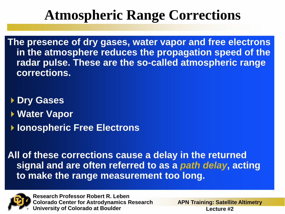
The presence of dry gases, water vapor and free electrons in the atmosphere reduces the propagation speed of the radar pulse. These are the so-called atmospheric range corrections.

Dry GasesWater VaporIonospheric Free Electrons

All of these corrections cause a delay in the returned signal and are often referred to as a path delay, acting to make the range measurement too long.



Atmospheric Range Corrections: Dry Gases

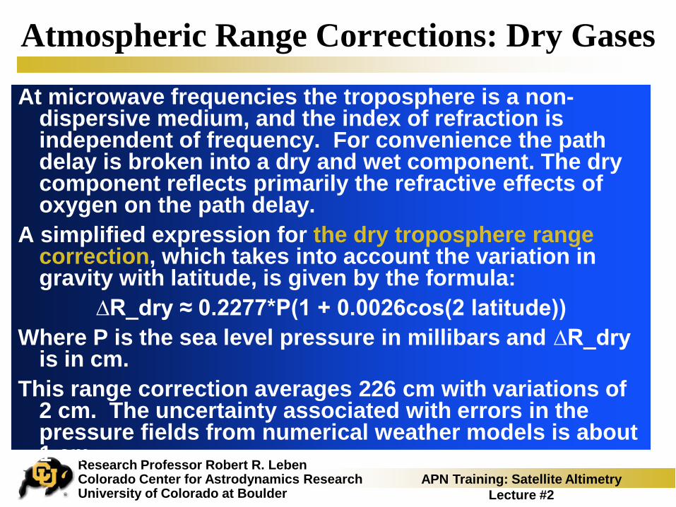
At microwave frequencies the troposphere is a non-dispersive medium, and the index of refraction is independent of frequency. For convenience the path delay is broken into a dry and wet component. The dry component reflects primarily the refractive effects of oxygen on the path delay.

A simplified expression for the dry troposphere range correction, which takes into account the variation in gravity with latitude, is given by the formula:

∆R_dry ≈ 0.2277*P(1 + 0.0026cos(2 latitude))Where P is the sea level pressure in millibars and ∆R_dry

is in cm.This range correction averages 226 cm with variations of

2 cm. The uncertainty associated with errors in the pressure fields from numerical weather models is about 1 cm.



Atmospheric Range Corrections: Water Vapor

The atmospheric range correction associated with columnar water vapor is called the wet troposphere correction and reflects water vapor and cloud liquid water droplet contributions to atmospheric refraction.

This effect is parameterized by empirical formula:∆R_wet ≈ 1.6 L

where L is the integrated columnar liquid water in gm/cm^2 and ∆R_wet has units of cm. �

This range correction averages 10 cm at high latitudes to 24 cm in tropical regions. Time variations are about 5 cm. The uncertainties is about 1 cm when corrected using a three-frequency microwave radiomenter.



TMR Water Vapor (g/cm2)



Microwave Radiometry

Modern altimeter rely on bore-sight radiometers to estimate the ∆R_wet.Algorithms using three frequency ( 18, 21 and 37 GHz)

brightness temperature trained on a large global database of radiosonde profiles to estimate ∆R_wet have accuracies of about 1 cm in rain free conditionsAlgorithms based on the two frequencies (23.8 and 36.5

GHz) used in the ERS radiometers have accuracies of about 2 cm rms.

Note: The ability to correct satellite altimeter data for water vapor attenuation requires coincident measurements from a passive microwave radiometer onboard the satellite because the columnar water vapor at any particular location varies with time.

This was an important lesson learned from GEOSAT.



Jason Microwave Radiometer (JMR)



Atmospheric Range Corrections: Ionospheric Free Electrons

Electrons liberated from atoms in the ionosphere by energetic solar radiation interact with microwaves to slow their propagation. Since the ionosphere is a dispersive medium, the refraction is a function of the frequency so that the free electron density can be calculated using the ranges measuremetns at different frequencies.

The ionosphere range correction is calculated from the total electron content unit (TECU) using the formula:

∆R_iono = 0.22 TECUwhere TECU is given in 10^16 electrons per meter^2 with

∆R_iono in cm.Like the wet troposphere correction, accurate

measurements of TECU are required for accurate altimetry given the time and space scales of ionospheric variability



Scales of the Ionospheric Delay

The ionosphere exhibits spatial and temporal variations that are difficult to reproduce with numerical models. Observations show:Mean values of the ionospheric delay range from 12 cm

near the equator to 6 cm at higher latitudes.Variations about the mean are as large as 5 cm near the

equator and 2 cm at higher latitudes. Meridional gradients as large as 2 cm per 100 km can

occur during mid to late afternoon at latitudes of 20° to 30°.Uncertainty in the measurements are about 1 cm after

smoothing the ionospheric correction at length scales less than 100 km.



Ionospheric Total Electron Content



Sea State Bias CorrectionsThe sea state bias is made up of two components Electromagnetic (EM) Bias - the difference between

mean sea level and the mean scattering surface.Skewness Bias - the difference between the mean

scattering surface and the median scattering surface.Recall that the returned signal measured by an altimeter is

the pulse reflected from the small wave facets within the antenna footprint that are oriented perpendicular to the incident wave fronts.

The shape of the returned waveform is thus determined from the distribution of these scatterers rather than the distribution of the actual sea surface height.

The half power point on the leading edge of the returned wave form corresponds to the median scattering surface.



External Geophysical Corrections

Geoid height - An accurate geoid is needed to calculate the total dynamic topography signal that includes both the mean ocean circulation and its variations. Early geoids have not been accurate enough for this application, however, by including gravity measurements form GRACE mission have reduced geoid errors at scales greater than 300 km so that scientifically useful information can be derived.Ocean and solid earth tidal height - Both ocean and

solid earth tides are measured by the altimeter and are considered noise on the non-tidal dynamical signal. Existing models derived from T/P data are accurate to better than 2 cm rms in the deep ocean.



Schematic of Ocean Circulation



Ocean Dynamic Topography



External Geophysical Corrections (cont.)

Atmospheric pressure loading - This is simply the depression of the sea surface by the atmosphere pressure force on the ocean surface. Spatial and temporal variations of this force are compensated partially by variations in the surface elevation. To first order, the ocean response as an “inverse barometer”, changing height by about one centimeter per milli bar of pressure change.

∆ IB (cm) ≈ 0.995 (P-1013)where P is the sea level pressure and 1013 is the mean sea level

pressure.In reality, the ocean responds both statically and dynamically

depending on the spatial and temporal scales of the forcing. Barotropic ocean signals, which are have significant power at

periods shorter than 20 days and are aliased by altimetric sampling, also an important external geophysical correction being studied. Barotropic ocean models forced with wind and pressure, however, are not sufficiently accurate reliable corrections for barotropic variability in routine altimeter data processing.



Instrument Corrections (some)Doppler shift - Doppler shifting of the transmitted chirp affects the

range calculation. This is corrected using the range rate, the rate of change of the range. Range rate is calculated in ground processing by least squares fitting of the range data over about 3 seconds of TOPEX data.

Range acceleration - The tracker algorithm is affected by the range acceleration. The range acceleration is calculated using the least squares employed for the range rate. Range rates can be as high as 10 meters per second^2 over ocean trenches.

Oscillator drift - any drift in the frequency of the oscillator direct affects the range calculated by counting cycles of the on board oscillator. This is calibrated by timing of telemetry signals at a ground receiving station. The distinction between frequency and counts per second resulted in an error in the ground based software for TOPEX causing a significant drift and bias in the altimeter measurement.

Pointing angle/sea state - the largest source of instrumental error is caused by of nadir pointing of the altimeter instrument. To varying degrees this affects the adaptive tracker unit (ATU) estimates of two-way travel time, the significant wave height and the sigma naught.



Some Jargon: Whatchu talkin’ ‘bout?

Dry tropo correctionWet tropo correction IB correction Iono correctionEM biasSkewness BiasSea State BiasOscillator driftPath delayGeoidDynamic topographyRange rateK.I.T.T. - Knight Industries 2000 (joke!)



Online References

CNES Radar Altimetry Toolboxhttp://www.altimetry.info/

WOCE/NASA Altimeter Algorithm Workshophttp://oceanesip.jpl.nasa.gov/sealevel/wocealt87.pdf

http://www.altimetry.info/�

http://oceanesip.jpl.nasa.gov/sealevel/wocealt87.pdf�

Documents

Altimeter Range Corrections - WordPress.com