ALTERNATIVE INDICES OF PERFORMANCE: AN …

AFRL-RH-WP-TR-2014-0095

ALTERNATIVE INDICES OF PERFORMANCE: AN EXPLORATION OF EYE GAZE METRICS IN A VISUAL PUZZLE TASK

Sheldon M. Russell, Gregory J. Funke, Brent T. Miller, Allen Dukes

Warfighter Interface Division

John M. Flach, Scott N.J. Watamaniuk Wright State University

Adam J. Strang

Consortium Research Fellows Program

Lauren Menke, Rebecca Brown Ball Aerospace & Technologies Corporation

July 2014 Interim Report

Distribution A: Approved for public release; distribution unlimited.

STINFO COPY

AIR FORCE RESEARCH LABORATORY 711 HUMAN PERFORMANCE WING,

HUMAN EFFECTIVENESS DIRECTORATE, WRIGHT-PATTERSON AIR FORCE BASE, OH 45433

AIR FORCE MATERIEL COMMAND UNITED STATES AIR FORCE

NOTICE AND SIGNATURE PAGE Using Government drawings, specifications, or other data included in this document for any purpose other than Government procurement does not in any way obligate the U.S. Government. The fact that the Government formulated or supplied the drawings, specifications, or other data does not license the holder or any other person or corporation; or convey any rights or permission to manufacture, use, or sell any patented invention that may relate to them. This report was cleared for public release by the 88th Air Base Wing Public Affairs Office and is available to the general public, including foreign nationals. Copies may be obtained from the Defense Technical Information Center (DTIC) (http://www.dtic.mil). AFRL-RH-WP-TR-2014-0095 HAS BEEN REVIEWED AND IS APPROVED FOR PUBLICATION IN ACCORDANCE WITH ASSIGNED DISTRIBUTION STATEMENT. //signed// //signed// KYLE L. TRAVER SCOTT M. GALSTER Work Unit Manager Chief, Applied Neuroscience Branch Applied Neuroscience Branch Warfighter Interface Division //signed// WILLIAM E. RUSSELL Chief, Warfighter Interface Division Human Effectiveness Directorate 711 Human Performance Wing Air Force Research Laboratory This report is published in the interest of scientific and technical information exchange, and its publication does not constitute the Government’s approval or disapproval of its ideas or findings.

http://www.dtic.mil/

REPORT DOCUMENTATION PAGE Form Approved OMB No. 0704-0188

The public reporting burden for this collection of information is estimated to average 1 hour per response, including the time for reviewing instructions, searching existing data sources, searching existing data sources, gathering and maintaining the data needed, and completing and reviewing the collection of information. Send comments regarding this burden estimate or any other aspect of this collection of information, including suggestions for reducing this burden, to Department of Defense, Washington Headquarters Services, Directorate for Information Operations and Reports (0704-0188), 1215 Jefferson Davis Highway, Suite 1204, Arlington, VA 22202-4302. Respondents should be aware that notwithstanding any other provision of law, no person shall be subject to any penalty for failing to comply with a collection of information if it does not display a currently valid OMB control number. PLEASE DO NOT RETURN YOUR FORM TO THE ABOVE ADDRESS. 1. REPORT DATE (DD-MM-YY) 2. REPORT TYPE 3. DATES COVERED (From - To)

01-07-2014 Interim 10 July 2013 – 30 April 2014

4. TITLE AND SUBTITLE ALTERNATIVE INDICES OF PERFORMANCE: AN EXPLORATION OF EYE GAZE METRICS IN A VISUAL PUZZLE TASK

5a. CONTRACT NUMBER In House

5b. GRANT NUMBER

5c. PROGRAM ELEMENT NUMBER 62202F

6. AUTHOR(S) Sheldon M. Russell1, Gregory J. Funke1, John M. Flach2, Scott N.J. Watamaniuk2, Adam J. Strang3, Brent T. Miller1,

Allen Dukes1, Lauren Menke4, and Rebecca Brown4

5d. PROJECT NUMBER 7184

5e. TASK NUMBER

5f. WORK UNIT NUMBER 71840877

7. PERFORMING ORGANIZATION NAME(S) AND ADDRESS(ES) 8. PERFORMING ORGANIZATION 2 Wright State University, Dept of Psychology, 3640 Col Glenn Highway, Dayton, OH 45435 3 Consortium Research Fellows Program, 4214 King St., Alexandria, VA 22302 4 Ball Aerospace & Technologies Corp., Systems Engineering Solutions; 2875 Presidential Drive, Suite 180; Fairborn, OH 45324-6269

REPORT NUMBER

9. SPONSORING/MONITORING AGENCY NAME(S) AND ADDRESS(ES) 10. SPONSORING/MONITORINGAir Force Materiel Command Air Force Research Laboratory 711 Human Performance Wing Human Effectiveness Directorate Warfighter Interface Division Applied Neuroscience Branch Wright-Patterson Air Force Base, OH 45433

AGENCY ACRONYM(S)AFRL/RHCP

11. SPONSORING/MONITORING AGENCY REPORT NUMBER(S)

AFRL-RH-WP-TR-2014-0095

12. DISTRIBUTION/AVAILABILITY STATEMENT Distribution A: Approved for public release; distribution unlimited.

13. SUPPLEMENTARY NOTES 88 ABW Cleared 09/08/2014; 88ABW-2014-4229. Report contains color.

14. ABSTRACT When an operator’s cognitive resources exceed demands, a ‘red line’ of performance may be crossed after which performance breaks down. Traditional approaches to

state assessment use secondary tasks (e.g., mental arithmetic) or secondary physiological measures (e.g., heart rate variability) for state assessment. The current work was motivated by dynamic systems theory which indicates that there are meaningful patterns of variability in ‘primary’ behaviors (e.g., required activities) which might provide a measure of operator state. The present work uses eye gaze as a primary measure in a visual puzzle task. The goal of Experiment 1 was to determine if performance changes in a visual puzzle task were reflected in eye gaze. The results of Experiment 1 suggest that there are impacts of task demands on gaze patterns, for both conventional and dynamic gaze metrics. There were also significant of practice that could be interpreted as learning or strategy shifts. The results of Experiment 2 show a significant improvement in performance in the task accompanied by change in gaze patterns; and that the dynamic measure of diagonal recurrence was systematically related to this performance change. This suggests that non-conventional measures of dynamic structure provide additional & complimentary information about operator state. 15. SUBJECT TERMS

Workload, Eye Tracking, Eye Movements, Nonlinear Dynamics

16. SECURITY CLASSIFICATION OF: 17. LIMITATION OF ABSTRACT:

SAR

18. NUMBER OFPAGES

55

19a. NAME OF RESPONSIBLE PERSON (Monitor) a. REPORT

Unclassified b. ABSTRACT Unclassified

c. THIS PAGE Unclassified

Kyle Traver 19b. TELEPHONE NUMBER (Include Area Code)

Standard Form 298 (Rev. 8-98) Prescribed by ANSI Std. Z39-18

i

TABLE OF CONTENTS

Section Page List of Figures .................................................................................................................... iii List of Tables ..................................................................................................................... iv 1.0 ABSTRACT ...............................................................................................................1 2.0 INTRODUCTION ……………………………………………………………… 2 2.1 Dynamic Approaches to Assessment .........................................................................5 2.1.1 Frequency Measures of Dynamic Structure ...............................................................5 2.1.2 Time Based Measures of Dynamic Structure ............................................................7 2.2 Eye Gaze: Dynamic Measures .................................................................................11 3.0 EXPERIMENT 1 .....................................................................................................15 3.1 Introduction ..............................................................................................................15 3.2 Methods....................................................................................................................17 3.2.1 Participants ...............................................................................................................17 3.2.2 Materials & Apparatus .............................................................................................17 3.2.3 Image Selection ........................................................................................................17 3.2.4 Procedure & Design .................................................................................................19 3.2.5 Dependent Variables ................................................................................................21 3.2.6 Calculation of Fixations ...........................................................................................22 3.2.7 Quantification of Dynamic Structure .......................................................................22 3.3 Results ......................................................................................................................23 3.3.1 Results for Trials 1 through 4 ..................................................................................23 3.3.2 Results for Trial 5 ....................................................................................................27 3.4 Discussion ................................................................................................................28 4.0 EXPERIMENT 2 .....................................................................................................30 4.1 Introduction ..............................................................................................................30 4.2 Methods....................................................................................................................30 4.2.1 Participants ...............................................................................................................30 4.2.2 Image Selection ........................................................................................................30 4.2.3 Apparatus .................................................................................................................31 4.2.4 Procedure and Design ..............................................................................................31 4.3 Results ......................................................................................................................32 5.0 GENERAL DISCUSSION ......................................................................................39 5.1 Task Demands & Gaze Patterns ..............................................................................39 5.2 Learning & Gaze Patterns ........................................................................................40 5.3 General Conclusions & Future Directions ...............................................................41 6.0 REFERENCES ........................................................................................................45

ii

LIST OF FIGURES

Figure Page

1. A conceptual diagram of the red line for workload and performance. ........................... 2 2. A randomly generated white noise time series (left) and Power Spectral Density Output (right). ................................................................................................................................. 6 3. A randomly generated pink noise time series (left) and Power Spectral Density Output (right).. ................................................................................................................................ 7 4. A randomly generated brown noise time series (left) and Power Spectral Density Output (right).. ................................................................................................................................ 7 5. a.) A random process plotted against itself.. ................................................................... 8 6. An example cross recurrence plot for two time series: Series 1 (Y-Axis) and Series 2 (X-Axis).. ................................................................................................................................ 10 7. An example cross recurrence plot for two time series: Series 1 (Y-Axis) and Series 2 (X-Axis).. ................................................................................................................................ 11 8. Eye gaze traces from Yarbus (1967).. ........................................................................... 13 9. Cross recurrence plot for one listener (Y-Axis) and speaker (X-Axis) dyad from the experiment conducted by Richardson & Dale, (2005).. .................................................... 15 10. Image pair 1 (Mountain Lake, Left; Sunflowers, Right).. .......................................... 18 11. Image pair 2 (Cleveland skyline, Left; Antique Printing Press, Right). ..................... 18 12. The image used for trial 5. .......................................................................................... 19 13. A diagram of the first four experimental trials, in one of two counterbalanced configurations. .................................................................................................................. 20 14. Average Fixation Length (Y-Axis) by Presentation (X-Axis) for two Counterbalanced Orders (dashed vs. solid lines). . ...................................................................................... 25 15. a.) β values (Y-Axis) by presentation (X-Axis) for Complex puzzles in two Counterbalanced Orders.................................................................................................... 26 16. The two images used between subjects in Experiment 2. ........................................... 31 17. Average Completion Time (Y-Axis) by Trial (X-Axis). ............................................ 33 18. Average Fixation Length (Y-Axis) by Trial (X-Axis).. .............................................. 35 19. Absolute β values (Y-Axis) by Trial (X-Axis). .......................................................... 36 20. Percent Diagonal Recurrence (Y-Axis) by Trial (X-Axis). ........................................ 37 21. Puzzle piece (Y-Axis) by position (X-Axis) Cross Recurrence matrix for one participant in the first learning trial. ................................................................................. 43 22. Puzzle piece (Y-Axis) by Position (X-Axis) Cross Recurrence matrix for one participant in the final learning trial.................................................................................. 44

iii

LIST OF TABLES

Table Page

1. An example of the experimental implementation for the first counterbalance type in Experiment 1. ....................................................................................................................... 20 2. Summary of dependent variables in Experiment 1. ......................................................... 21 3. Summary of significant main effects of Task Demands for trials 1-4. ............................ 24 4. Summary of significant main effects of Practice for trials 1-4. ....................................... 26 5. Summary of significant results for Trial 5. ...................................................................... 27 6. Summary of significant main effects for paired difficulty comparisons with and without the secondary task. ............................................................................................................... 28 7. Summary of dependent variables tested in Experiment 2. ............................................... 33 8. Summary of model fits for the hypothesized effects in Experiment 2. ........................... 34 9. Average correlation coefficients for the dependent variables tested in Experiment 2. ... 38 10. Summary of results for a subset of data from the first experiment, split by successful puzzle completion ................................................................................................................ 42

iv

1.0 ABSTRACT

Of interest to the U.S. Air Force is the ability to develop and characterize the level of workload that operators are under at any given point. When an operator’s cognitive resources exceed demands, a ‘red line’ of performance may be crossed after which performance breaks down. What is needed is an estimate of operator state; a ‘dipstick’ for the operator in order to assess the level of ‘resources’ available, in order to avoid performance problems. Traditional approaches use secondary tasks (e.g., mental arithmetic) or secondary physiological measures (e.g., heart rate variability) for state assessment. However, the current work was motivated by dynamic systems theory which indicates that there are meaningful patterns of variability in ‘primary’ behaviors (e.g., required activities) which might provide a measure of operator state. The present work uses eye gaze as a primary measure in a visual puzzle task. The link between eye gaze and attention is generally accepted as is the link between attention and performance outcomes. The goal of Experiment 1 was to determine if performance changes in a visual puzzle task were reflected in eye gaze, as measured in multiple ways: Conventional (e.g., average fixation length) & dynamic (e.g., β values, measures derived from a recurrence matrix). These relationships were explored in relation to task difficulty, time on task, as well as spare capacity. The results of Experiment 1 suggest that there are impacts of task demands on gaze patterns, for both conventional and dynamic gaze metrics. There were also significant of practice on eye gaze patterns in Experiment 1 that could be interpreted as learning or strategy shifts. The impact of learning on eye gaze was explored in a follow up experiment. The results of Experiment 2 show a significant improvement in performance in the task accompanied by change in gaze patterns when repeating the same puzzle; and that the dynamic measure of diagonal recurrence was systematically related to this performance change. This suggests that non-conventional measures of dynamic structure provide additional & complimentary information about operator state.

1 Distribution A: Approved for public release; distribution unlimited.

88 ABW Cleared 09/08/2014; 88ABW-2014-4229.

2.0 INTRODUCTION

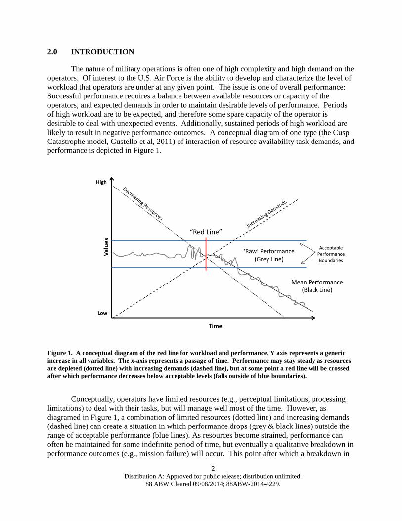
The nature of military operations is often one of high complexity and high demand on the operators. Of interest to the U.S. Air Force is the ability to develop and characterize the level of workload that operators are under at any given point. The issue is one of overall performance: Successful performance requires a balance between available resources or capacity of the operators, and expected demands in order to maintain desirable levels of performance. Periods of high workload are to be expected, and therefore some spare capacity of the operator is desirable to deal with unexpected events. Additionally, sustained periods of high workload are likely to result in negative performance outcomes. A conceptual diagram of one type (the Cusp Catastrophe model, Gustello et al, 2011) of interaction of resource availability task demands, and performance is depicted in Figure 1.

Figure 1. A conceptual diagram of the red line for workload and performance. Y axis represents a generic increase in all variables. The x-axis represents a passage of time. Performance may stay steady as resources are depleted (dotted line) with increasing demands (dashed line), but at some point a red line will be crossed after which performance decreases below acceptable levels (falls outside of blue boundaries).

Conceptually, operators have limited resources (e.g., perceptual limitations, processing limitations) to deal with their tasks, but will manage well most of the time. However, as diagramed in Figure 1, a combination of limited resources (dotted line) and increasing demands (dashed line) can create a situation in which performance drops (grey & black lines) outside the range of acceptable performance (blue lines). As resources become strained, performance can often be maintained for some indefinite period of time, but eventually a qualitative breakdown in performance outcomes (e.g., mission failure) will occur. This point after which a breakdown in

Acceptable Performance Boundaries

“Red Line”

Mean Performance (Black Line)

‘Raw’ Performance (Grey Line)

Time

Low

High

Valu

es


88 ABW Cleared 09/08/2014; 88ABW-2014-4229.

performance is inevitable can be characterized as a ‘red line’ (Grier et al., 2008). Avoiding the ‘red line’ is critical; typical military tasks are in domains in which performance failures are at a minimum undesired (e.g., transportation delays) and potentially catastrophic (e.g., air traffic control accident, loss of life or critical equipment). What is needed is a ‘dipstick’ for the operator; some way to gain information about the level of ‘resources’ available at any given point.

The issue is certainly multifaceted, and there has been a large body of work in this area

(e.g., Tsang & Vidulich, 2006). However, the focus of the present work is not to classify or model the source(s) of workload, but rather to approach the problem more generally in regards to how the state of the operator might be influenced by task demands in a way that is detectable by some parameter or measurement from the operator. This could provide an objective indication of operator state, as opposed to a subjective indicator derived via questionnaires (e.g., NASA Task Load Index; Hart and Staveland, 1988). At a minimum, a signal needs to be loosely coupled to performance outcomes. In order to be useful from an operational standpoint, it also needs to be relatively unobtrusive to collect. Ideally, this measurement would allow for a prediction of a future qualitative change in performance outcomes.

The research strategy adopted by the Applied Neuroscience Branch of the Air Force is

the Sense-Assess-Augment framework (Parasuraman & Galster, 2013). First, provide adequate sensor capability to measure the appropriate phenomena or parameters to detect the underlying state (Sense); analyze the data in such a way as to gain insight into the underlying state of the operator in relation to performance (Assess); and finally provide corrective action or intervention if needed (Augment). The general goal is to find a signal which is ‘loosely coupled’ to performance: For predictive purposes, quantitative changes in the signal should be evident even if overall performance is remaining constant. Prior to the red line, a critical value in the signal should readily identify an upcoming qualitative performance change. For the present work, the term operator state assessment will be used to represent this idea; to measure a parameter or signal from the operator which relates the availability of ‘resources’ in order to predict performance.

A common approach to assessment is the addition of a secondary task (e.g., mental

arithmetic, tracking tasks, etc.) to the primary task of interest. A dual-task paradigm allows for measurement of performance for both primary & secondary tasks and by manipulating the difficulty of one of the tasks, changes in the other can be used to estimate levels of spare capacity. While this method has been shown to be effective in laboratory settings, (e.g., Ogden et al, 1979; O’Donnell & Eggemeier, 1986) the ability to make assessments of operator state comes at the cost of adding more work for the operator, which is undesirable in typical operational settings.

Physiological signals represent another type of measurement that has been hypothesized

to reflect to the state of the operator, and multiple physiological signals have been studied. A short list, certainly not all inclusive, includes heart rate variability (HRV; reviewed by Jorna, 1992), brain activity as measured by electro encephalogram (EEG; Wilson, 2002), and cerebral blood flow velocity (reviewed by Warm, Parasuraman, & Matthews, 2008). Each has been


88 ABW Cleared 09/08/2014; 88ABW-2014-4229.

shown to be related with performance outcomes in some way (e.g., vigilance decrement and blood flow velocity), but these relationships are not definitive. Drawbacks in regards to lack of sensitivity to workload changes (HRV), signal/noise problems (EEG), and intrusiveness or feasibility of implementation (cerebral blood flow) have limited the overall success in both laboratory and operational settings. With additional research and technological innovation these limitations may be overcome; however at present research in the field of complexity and nonlinear dynamics may provide an alternative way to assess the state of the operator from primary measures of behavior, rather than ‘secondary’ physiological measures or tasks.

Consider ‘raw performance’ diagrammed in Figure 1 (grey line). Mean performance

(black line) may be stable, but there will be variability in performance. Assumptions of central tendency consider this variability as error (i.e. variability carries little information about the source). However, measures of variability in a wide variety of natural and manmade phenomena (e.g., forest fires, avalanches, water levels in lakes, traffic patterns on the road, traffic on telephone lines; Jensen, 1998; Newman, 2005) indicate that there are specific patterns of variability in ‘primary’ measures of phenomena that represent underlying states of the overall system (e.g., day to day variability in water levels provides insight into the overall properties of the lake, such as drought conditions). Research in dynamic systems suggests that variability is not necessarily random; in the examples mentioned above there are meaningful, complex patterns in behavior which are often revealed by time series analyses (a time series is the time ordered series of repeated measurements for an entire data collection epoch). Key to the issue of state assessment is that variability patterns measured in a primary signal (e.g., a primary task performance activity) can reflect the qualitative state of the system as a whole (such as approaching the red line).

From a dynamical systems perspective, the assumption is that any type of complex

system will have interactions between underlying components and processes that will influence the measured outcome (e.g., Takens 1981). The effects of these interactions only become apparent when data is observed across time (rather than collapsed in time as with an average). In general terms from complexity theory, dynamic systems exhibit a variable, yet globally stable ‘macrostructure’ (e.g., performance or behavior) coupled to a highly variable ‘microstructure’ (e.g., components or processes) (Kelso, 2005, Kloos and Van Orden, 2010). Note that complexity theory is somewhat agnostic to what the components are; analyzing data across time often reveals properties of the coupling and interactions between components and processes without identification of the components themselves.

Motivated by these broader patterns in nature (e.g., self-organization and spontaneous

order; Kugler, Kelso & Turvey, 1982), Kelso demonstrated that qualitative ‘phase shifts’ in performance can be measured by quantitative analysis of variability patterns over time. Kelso demonstrated these complex phase-shift relationships with a model system: finger tapping. Participants were asked to move both their left and right index fingers with a metronome. Participants tended to exhibit one of two stable tapping states between their fingers: Either in-phase (both index fingers ‘up’ then both ‘down’) or anti-phase (one finger up, the other down). Participants were allowed to move their fingers in whichever orientation was ‘comfortable’. As the metronome speed was increased, fluctuations, or phase shifts, between the two patterns began


88 ABW Cleared 09/08/2014; 88ABW-2014-4229.

to occur. Each phase shift was preceded by spikes in variability (critical fluctuations), or a regularity or periodicity (critical slowing down) in the variability patterns of the primary time series (Kelso, 1995).

Kelso’s body of work on phase transitions has motivated and informed other areas of

human performance. For example, qualitative shifts in movement (e.g., from walking to running), can be measured by the variability patterns in the coordination of limbs (Harrison & Richardson, 2009). When two individuals are “harnessed” together, a qualitative shift into organized quadrupedal movement between the two individuals is established, as quantified by a change in variability in the limb movements between the two individuals (Harrison & Richardson, 2009). Crites and Gorman (2013) report different patterns of variability in novel vs. existing skill acquisition. In addition to motor control research, Van Orden et al (2005) show that primary measures of reaction time exhibit specific patterns of variability, which is thought to be inherent to normal cognitive performance. Taken together, there is evidence suggesting that critical patterns of variability in primary measures can describe qualitative shifts in behavior, and furthermore that changes in variability patterns may precede these shifts. If future qualitative shifts in operator state can quantified by patterns of variability exhibited in the behavior itself it may provide an alternative approach for state assessment.

2.1 Dynamic Approaches to Assessment

Regardless of the choice of signal, an important analytical question is how to quantify the signal in a way that represents the state of the operator in a meaningful way. As previously mentioned, conventional approaches to this problem quantify signals in some type of average value (e.g., average HRV in a frequency band (Jorna, 1992); average EEG activity (Wilson, 2002)). Certainly measuring average values will be important information for state assessment (or any type of data analysis), but given the potential benefit of time series analyses it makes sense to also measure patterns over time.

The following examples are methods for analyzing data via time series analysis, and are

presented as demonstrations of their respective types of variability, or dynamic structure. It is generally expected that patterns of behavior emerge and change over the course of learning and experience (Warren, 2006; Davids et al, 2008) and are constrained by both intrinsic (internal) and extrinsic (task) dynamics (Holden, Choi, Amazeen, & Van Orden, 2011; Kloos and Van Orden, 2010; Kelso, 1995). In other words, by manipulating external constraints in an experimental context, changes to internal constraints are likely to result, and these changes are likely to be measured by time series analyses of the signal. For the present work, analyses in both the frequency and time domains were used in order to leverage multiple measures of dynamic structure.

2.1.1 Frequency Measures of Dynamic Structure

Frequency analyses assess the level of dynamic structure based on the amount of randomness vs. dependence that is present in the data. Frequency analyses, specifically power spectral density (PSD) correlations of frequency to absolute power, as computed through the Fast Fourier Transform (FFT), make distinctions about the level of randomness and structure in a


88 ABW Cleared 09/08/2014; 88ABW-2014-4229.

time series. When the PSD output is converted to logarithmic scales, a regression fit is computed. The slope of the regression equation is a measure of the relationship between the frequency and power exhibited by the time series, which indicates the level of persistence observed in the time series. Persistence can be thought of as the degree to which values depend on previous values (i.e. dependence). For complex systems, the regression relationship is a power law fit. The slope values reported are referred to as scaling exponents, or β values (Eke et al., 2002).

Slopes (β values) calculated at or near zero are indicative of random processes, or white

noise processes, in which all observed frequencies have equal power, as shown in Figure 2. As the frequency to power relationship inverts, such that lower frequencies show proportionally higher power, negative slope values are observed. Negativeβ values between -.5 to -1.5, are indicative of a specific type of persistence called pink noise or 1/f noise, shown in Figure 3. Rather than all frequencies exhibiting equal power, for 1/f noise power and frequency are inversely related such that lower frequencies show greater power and vice versa. Figure 4 depicts a time series with even greater dependence, as indicated by β values between -1.5 to -2.5 which are often referred to as brown noise. Most time series of human phenomena exhibit β values which can be described as fitting one of these three categories (white noise, 1/f noise, brown noise). Note that in all cases presented here, the mean value for the time series is zero: The obvious qualitative differences between the examples are revealed by time series analysis, as opposed to averages.

Figure 2. A randomly generated white noise time series (left) and Power Spectral Density Output (right). β = 0 indicates no correlation among frequency (y axis) and power (x axis). Note that the time series has a mean of zero and a standard deviation of 1.

-4

-3

-2

-1

0

1

2

3

4

β = -0.0601x

-3

-2

-1

0

1

2

3

-3 -2.5 -2 -1.5 -1 -0.5 0

White Noise


88 ABW Cleared 09/08/2014; 88ABW-2014-4229.

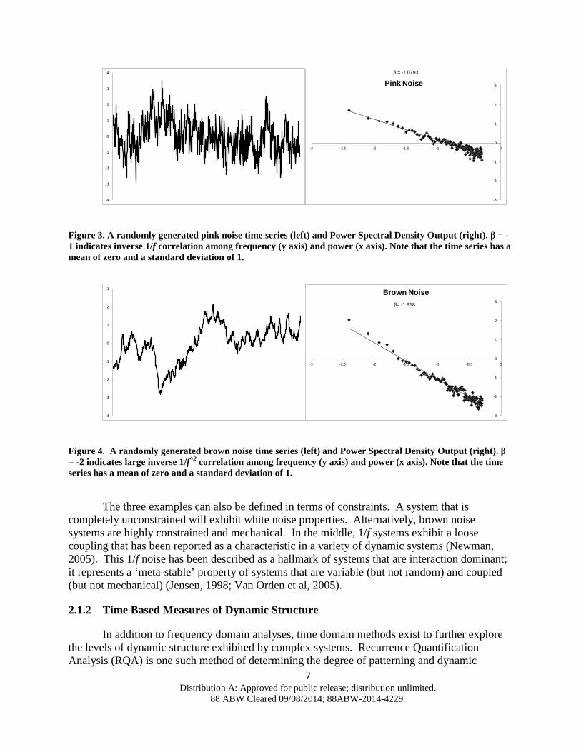
Figure 3. A randomly generated pink noise time series (left) and Power Spectral Density Output (right). β = -1 indicates inverse 1/f correlation among frequency (y axis) and power (x axis). Note that the time series has a mean of zero and a standard deviation of 1.

Figure 4. A randomly generated brown noise time series (left) and Power Spectral Density Output (right). β = -2 indicates large inverse 1/f^2 correlation among frequency (y axis) and power (x axis). Note that the time series has a mean of zero and a standard deviation of 1.

The three examples can also be defined in terms of constraints. A system that is completely unconstrained will exhibit white noise properties. Alternatively, brown noise systems are highly constrained and mechanical. In the middle, 1/f systems exhibit a loose coupling that has been reported as a characteristic in a variety of dynamic systems (Newman, 2005). This 1/f noise has been described as a hallmark of systems that are interaction dominant; it represents a ‘meta-stable’ property of systems that are variable (but not random) and coupled (but not mechanical) (Jensen, 1998; Van Orden et al, 2005).

2.1.2 Time Based Measures of Dynamic Structure

In addition to frequency domain analyses, time domain methods exist to further explore the levels of dynamic structure exhibited by complex systems. Recurrence Quantification Analysis (RQA) is one such method of determining the degree of patterning and dynamic

-4

-3

-2

-1

0

1

2

3

4 β = -1.0793

-3

-2

-1

0

1

2

3

-3 -2.5 -2 -1.5 -1 -0.5 0

Pink Noise

-4

-3

-2

-1

0

1

2

3

β= -1.918

-3

-2

-1

0

1

2

3

-3 -2.5 -2 -1.5 -1 -0.5 0

Brown Noise


88 ABW Cleared 09/08/2014; 88ABW-2014-4229.

structure in a time series. Essentially, an N × N matrix plot (where N is the time series length; the simplest method plots a time series against itself) is generated. As depicted in Figure 5a and b, any shaded area represents a “match” or recurrent point. The ratio and locations of these recurrent points provide the basic units of analysis in this method. The first of these metrics is percent recurrence (%REC) which is the ratio of recurrent points, to all possible points. Percent recurrence represents the proportion of “states” that repeat or recur across the time series. A second measure, percent determinism (%DET), is the percentage of recurrent states that repeat in the same order each time; deterministic points appear as diagonal line structures in the matrix. Note the large diagonal in the center which splits the plot into two identical halves. For, RQA the plot is one to one on the time series to itself (i.e., the diagonal is not meaningful; a time series will always be identical with itself along the center diagonal) and only half of the plot is used for computation.

Similar to the previous frequency analysis examples, RQA can describe the

characteristics of the system that produced the time series. Webber and Zbilut (2005) note that an unconstrained or white noise (e.g., random process; Figure 5a) system will show random levels of recurrence & determinism that are at chance levels. Highly constrained systems (e.g., a sine wave; Figure 5b) will produce very high values for %REC and %DET as the system repeats the same patterns in the same order. Between these two extremes, loosely constrained systems will show moderate patterning; they exhibit greater than chance levels of recurrence and determinism, but not at extreme levels that would be seen in highly mechanical systems.

Figure 5. a.) A random process plotted against itself. Shaded areas represent recurrent points; which occur as a matter of chance, as do diagonal line structures. b.) A sine wave plotted against itself. Shaded areas represent recurrent points, which always occur in the same period as the sine wave itself; nearly all points fall on a diagonal line structure.

N-Rand

N-Ra

nd

N-Sine

N-Si

ne

a.) b.)


88 ABW Cleared 09/08/2014; 88ABW-2014-4229.

A standard RQA provides an estimate of dynamic structure in a system using a single variable; however the mathematics are equally able to provide estimates of structure and coupling between two variables (or systems). In this method, Cross Recurrence Quantification Analysis (CRQA; Weber & Zbilut, 2005), the same metrics from a standard RQA are computed, but for a matrix that compares two different time series (e.g., an N1 × N2 matrix), as shown in Figure 6 and Figure 7. Rather than define self-similar patterns of dynamic structure (RQA), higher levels of cross recurrence (%CREC) indicate similarity between the two time series (e.g., when there is a dot in the matrix the two time series shared the same value) and %CDET is a general indicator of coupling between the two time series (still visible as diagonal lines in the matrix).

CRQA provides a third way to further quantify the level of coupling between two time

series. Whereas a standard RQA has a diagonal that is not meaningful at a time lag of zero, a diagonal line at lag zero in a CRQA is a further indication of the level of synchronized coupling of the two time series (Dale, 2011). Analysis of the Diagonal Recurrence Profile (DRP) is similar to an autocorrelation function. The diagonal recurrence profile computes the percentage of values that recur along different levels of “lag”. Lag 0 is computed along the diagonal (e.g., do the two time series have the same value at the same time). A lag of 1 would compute the proportion at +/- 1 measurement in the time series from time zero and so on (e.g., a state that occurs at time x in N1 recurs at time x + 1 in N2). As shown in Figure 6, higher levels of diagonal recurrence (%DREC) along a lag of zero indicate a high level of synchronicity between the two time series. Figure 7 shows a cross recurrence matrix for two times series that exhibit low levels of similarity and coupling. Time series that are not strongly coupled will show low levels of %DREC at all lag values. Although the present work will focus on a %DREC at a lag of zero, it should be noted that high %DREC at lag values other than zero could be indicators of coupling between the time series in a leader/follower relationship (Richardson & Dale, 2005).


88 ABW Cleared 09/08/2014; 88ABW-2014-4229.

Figure 6. An example cross recurrence plot for two time series: Series 1 (Y-Axis) and Series 2 (X-Axis). Shaded grey areas represent matching values between the two series (recurrence). Line structures (an example is circled in red) represent matching values in an order (determinism). Diagonal Recurrence appears as a line structure along the diagonal. The high level of diagonal recurrence presented in this figure indicates high (but not total) coupling between the two time series.

Serie

s 1

Series 2


88 ABW Cleared 09/08/2014; 88ABW-2014-4229.

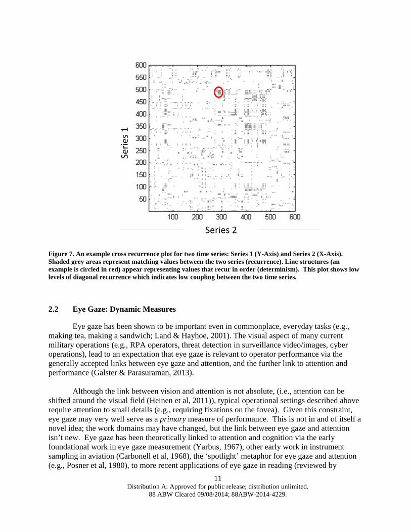
Figure 7. An example cross recurrence plot for two time series: Series 1 (Y-Axis) and Series 2 (X-Axis). Shaded grey areas represent matching values between the two series (recurrence). Line structures (an example is circled in red) appear representing values that recur in order (determinism). This plot shows low levels of diagonal recurrence which indicates low coupling between the two time series.

2.2 Eye Gaze: Dynamic Measures

Eye gaze has been shown to be important even in commonplace, everyday tasks (e.g., making tea, making a sandwich; Land & Hayhoe, 2001). The visual aspect of many current military operations (e.g., RPA operators, threat detection in surveillance video/images, cyber operations), lead to an expectation that eye gaze is relevant to operator performance via the generally accepted links between eye gaze and attention, and the further link to attention and performance (Galster & Parasuraman, 2013).

Although the link between vision and attention is not absolute, (i.e., attention can be

shifted around the visual field (Heinen et al, 2011)), typical operational settings described above require attention to small details (e.g., requiring fixations on the fovea). Given this constraint, eye gaze may very well serve as a primary measure of performance. This is not in and of itself a novel idea; the work domains may have changed, but the link between eye gaze and attention isn’t new. Eye gaze has been theoretically linked to attention and cognition via the early foundational work in eye gaze measurement (Yarbus, 1967), other early work in instrument sampling in aviation (Carbonell et al, 1968), the ‘spotlight’ metaphor for eye gaze and attention (e.g., Posner et al, 1980), to more recent applications of eye gaze in reading (reviewed by

Serie

s 1

Series 2


88 ABW Cleared 09/08/2014; 88ABW-2014-4229.

Rayner, 1998), and general work regarding eye movements (Kowler, 2011). While the interest in eye gaze and the links to attention are not new topics, the capability to readily measure and record eye movements unobtrusively and in operation settings is a more recent capability that could be implemented for purposes of state assessment (Duchowski, 2002).

In addition to the previous examples linking eye gaze to performance, eye gaze measures

have been linked to operator workload. May et al (1990) report a decrease in the number and range of eye movements during free view when participants performed a secondary counting task. The range showed further reduction as secondary task difficulty was increased. In a more applied setting, driving, a narrowing of visual attention, or “tunnel vision”, has been observed under high workload (e.g., Reimer, 2009). Tunnel vision is often accompanied by an increase in the number of fixations, and a corresponding decrease in the length of fixation. It would then be expected that by manipulating task difficulty in an experiment, that changes in gaze patterns will likely result.

Yarbus’ (1967) work on eye gaze patterns in complex scene viewing provides further

foundation for the expectation that simple changes in experimental context can produce vast differences in gaze patterns. Yarbus was one of, if not the first, to measure gaze patterns using an eye tracking apparatus. Yarbus showed participants a series of images, while tracking eye gaze. Yarbus provided different questions about the image for participants to ‘keep in mind’ while viewing the images. A sample image, “The Unexpected Visitor”, is depicted in Figure 8 illustration adapted from Yarbus, 1967; figure from Land & Tatler, 2009).


88 ABW Cleared 09/08/2014; 88ABW-2014-4229.

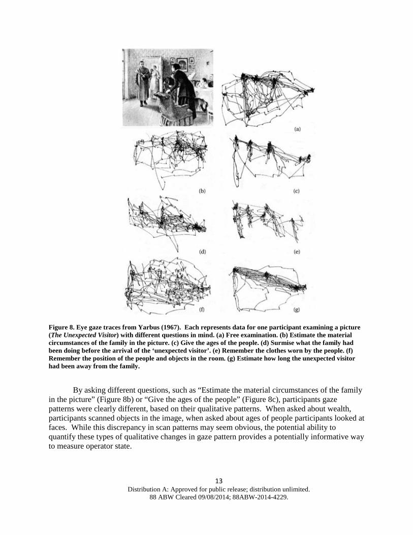
Figure 8. Eye gaze traces from Yarbus (1967). Each represents data for one participant examining a picture (The Unexpected Visitor) with different questions in mind. (a) Free examination. (b) Estimate the material circumstances of the family in the picture. (c) Give the ages of the people. (d) Surmise what the family had been doing before the arrival of the ‘unexpected visitor’. (e) Remember the clothes worn by the people. (f) Remember the position of the people and objects in the room. (g) Estimate how long the unexpected visitor had been away from the family.

By asking different questions, such as “Estimate the material circumstances of the family in the picture” (Figure 8b) or “Give the ages of the people” (Figure 8c), participants gaze patterns were clearly different, based on their qualitative patterns. When asked about wealth, participants scanned objects in the image, when asked about ages of people participants looked at faces. While this discrepancy in scan patterns may seem obvious, the potential ability to quantify these types of qualitative changes in gaze pattern provides a potentially informative way to measure operator state.


88 ABW Cleared 09/08/2014; 88ABW-2014-4229.

Again, conventional approaches to quantifying eye movements in tasks that involve active participation of the participant (e.g., active tasks) include average fixation length or average movement velocity (e.g., May et al, 1990; Hayhoe et al, 1998; Kowler, 2011). As has been stated, this type of approach likely misses potentially informative information from variability patterns in eye gaze time series.

Initial research using time history analyses (utilizing measures of dynamic structure) has

been conducted by Aks et al. (2002). Similar to other complex systems, visual search involves many interacting processes and components, including the influences of the experimental task, leading Aks et al. to hypothesize that eye gaze time series would exhibit dynamic structure in a visual search task. The task used was searching for a target (uppercase T) among distracters (upper case E). The results indicate that Euclidian distance between subsequent measurements (X1-X2 and Y1-Y2 pixel position) recorded in visual search tasks exhibit temporal structure in the range of brown noise (β ≈ -2). This initially suggested a high level of dependence between fixations. There was some concern that position data alone could produce spurious brown noise, due to constraints that the screen size imposed on the gaze time series. This led the researchers to further analyze an additional metric, angular change between eye movements. Angular change measures the difference between subsequently tracked positions in angular units rather than distance units. When the raw gaze time series were converted to angular changes between positions, the analysis revealed a 1/f (β ≈ -1) correlation.

Stephen and Anastas (2011) re-analyzed data from an earlier publication (Stephen and

Mirman, 2010) and confirmed findings of Aks et al. (2002), in regards to dynamic structure observed in eye movement time series. However, Stephen and Anastas (2011) went a bit further, by analyzing the relationship between dynamic structure and reaction time using growth curve modeling. The data suggests that dynamic structure for angular-change time series that exhibit patterns of 1/f noise are related to decreases in reaction time; an improvement in the performance measure for the task.

Frequency analyses provide a general classification of eye gaze (e.g., random vs.

structured), but this general classification is likely complimented by more explicit measures of coupling and similarity from time domain measures of cross recurrence. Richardson and Dale (2005) used cross recurrence of eye gaze time series as a way to understand the coupling between speakers and listeners when telling a story. Two participants had separate screens with identical depictions of characters from a popular television show. One participant told a predetermined story about an episode of the television show (speaker). The listener had to respond to a series of questions about this story. Both participants’ gaze was tracked while the story was told, and was analyzed via cross recurrence. Listeners whose gaze patterns showed higher coupling with gaze patterns of speakers (as measured through % Diagonal Recurrence) also exhibited better retention when asked questions about the story. Figure 9 depicts a sample cross recurrence plot for a listener/speaker dyad as presented in Richardson and Dale (2005) with relatively strong coupling in their eye gaze patterns.


88 ABW Cleared 09/08/2014; 88ABW-2014-4229.

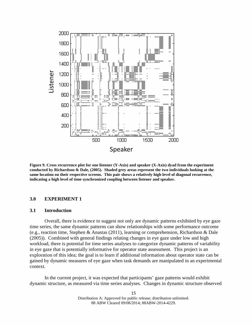
Figure 9. Cross recurrence plot for one listener (Y-Axis) and speaker (X-Axis) dyad from the experiment conducted by Richardson & Dale, (2005). Shaded grey areas represent the two individuals looking at the same location on their respective screens. This pair shows a relatively high level of diagonal recurrence, indicating a high level of time synchronized coupling between listener and speaker.

3.0 EXPERIMENT 1

3.1 Introduction

Overall, there is evidence to suggest not only are dynamic patterns exhibited by eye gaze time series, the same dynamic patterns can show relationships with some performance outcome (e.g., reaction time, Stephen & Anastas (2011), learning or comprehension, Richardson & Dale (2005)). Combined with general findings relating changes in eye gaze under low and high workload, there is potential for time series analyses to categorize dynamic patterns of variability in eye gaze that is potentially informative for operator state assessment. This project is an exploration of this idea; the goal is to learn if additional information about operator state can be gained by dynamic measures of eye gaze when task demands are manipulated in an experimental context.

In the current project, it was expected that participants’ gaze patterns would exhibit

dynamic structure, as measured via time series analyses. Changes in dynamic structure observed

List

ener

Speaker


88 ABW Cleared 09/08/2014; 88ABW-2014-4229.

in eye movement time series are likely indicative of the underlying organizational and structural changes within the cognitive and visual systems. Both frequency and time based measures of dynamic structure were tested. These alternative indices were expected to provide additional information when compared to conventional (average based) measures of eye gaze behavior (e.g., average fixation time). As task demands shift, and participants adapt, qualitative gaze behavior is likely to shift (e.g., Kelso, 2005, Kloos & Van Orden, 2012). This is likely to be reflected in the properties of dynamic patterns; resulting in different, but stable patterns of variability (e.g., β & Cross Recurrence values change).

The current study measured eye gaze in a visual task with a cognitive component.

Specifically, the task was a visual puzzle task in which participants were asked to unscramble an image. Given the nature of the task, eye gaze is considered a primary measure of performance. This type of task provided a way to manipulate task demands by changing the constraints of task difficulty, practice, and the addition of a secondary task. Task difficulty was manipulated by changing the way in which the image can be scrambled; in one condition puzzle pieces had the potential for rotation. This manipulation provided a way to control for any potential difficulty effects of any individual image, while still manipulating task difficulty (i.e. the information content of each piece of the puzzle) in a significant way. Multiple trials of the same difficulty level allowed for potential changes in dynamic structure due to learning or strategy (i.e., practice effects) to be observed. Finally, aside from general task difficulty, a secondary task was implemented to further tax participants’ attention and capacity.

As a first step in using eye gaze for state assessment, the current project tested discrete

levels of task difficulty (as opposed to a continuous increase in difficulty), as a way to determine if differences in eye gaze exist that could be representative of a ‘pre’ and ‘post’ red line situation. Rather than stipulate explicit directional hypotheses, the current questions are explicitly two tailed. It is difficult to specify a direction of the changes in dynamic structure at the outset of this project. Changes in task demands could create disruptions (i.e. critical fluctuations add noise to the system) and as a result randomness (e.g., a ‘whitening’ of the time series) could be observed. Alternatively, changes in task demands could further constrain the possibilities for action; this would result in higher levels of dynamic structure in eye movements (i.e. critical fluctuations; system becomes more periodic). Either direction provides insight into underlying processes, and potential classification of the operator.

Practice effects may also further influence dynamic patterns observed, however it is also

difficult to specify a specific direction of change in dynamic structure. A serial or other highly structured scan path could be implemented early in learning, and with learning participants could shift to a less constrained scan path. Alternatively, scan paths could initially exhibit more randomness, and show an increase in structure. Again, either direction could provide insight into the underlying state of the operator.


88 ABW Cleared 09/08/2014; 88ABW-2014-4229.

3.2 Methods

3.2.1 Participants

Thirty-two total participants with ages ranging from 18-30 years from a Midwestern university population were recruited to participate and were compensated with course credit or were paid $30. One participant was dropped due to a calibration error with the eye tracking equipment. Thirty-one total participants are included in the subsequent analysis. Biographic information was collected via self-report questionnaire. There were 14 male and 17 female participants with a median age of 23. All reported normal or corrected to normal vision. Highest education level completed was as follows: High School (15), associate’s degree (3), bachelor’s degree (7), and graduate degree (6). Experience with video games was assessed, with a range of 0 to 16 hours per week reported, with an average of 3.16 (SD = 3.2) hours of video game play per week.

3.2.2 Materials & Apparatus

Eye gaze was measured via a Facelab4 “off the head” eye tracker, hosted on a Dell Latitude D830 laptop computer (2.2 GHz processor, 2 GB RAM). This combination allowed for +/- 1 degree of visual angle eye tracking capability at a collection rate of 60Hz. Facelab API v4.6 (reference) was integrated with custom software written to display images for this experiment. The output of the tracking software was the X and Y pixel location of participants’ gaze every 16.7 ms. The participant station was an HP Compaq DC80 desktop computer (2.3 GHz processor, 3.5 GB RAM) & a LCD monitor (Samsung 940BX) with a screen area of 30cm by 37.5cm (48cm diagonal), and a resolution of 1280 x 1024 pixels.

Images were sized at 1020 x 1020 pixels, which at a viewing distance of approximately

60cm, is approximately 27 degrees of visual angle. When subdivided into 36 equal sized square pieces for the puzzle each piece was 170 pixels square. At a 60cm viewing distance, each puzzle piece subtended approximately 4.5 degrees of visual angle.

3.2.3 Image Selection

Initial images were selected from public domain sources (e.g., Wikipedia). Images containing human faces were excluded. In addition, all images were selected to contain a “natural” correct orientation. Early pilot testing of “non-oriented” still life images suggested that a participant in the rotated condition could solve the puzzle such that the pieces appeared to be correctly matching yet the entire puzzle was rotated (i.e. the puzzle was put together in a way that all the pieces ‘matched’, but were all upside down). Twelve images meeting these criteria were initially selected.

In order to select the five images needed for Experiment 1, the 12 images were pilot

tested by 4 participants meeting the recruitment requirements described above. Participants unscrambled all 12 images in a randomized order for the standard puzzle condition (see below). Images were then ranked based on average time to completion. Time series analyses require a minimum number of samples for a valid analysis, therefore the five images that had the longest


88 ABW Cleared 09/08/2014; 88ABW-2014-4229.

completion times were chosen, provided they were solved by all pilot participants. To determine if there were any rank differences between participants, these five images were subjected to a nonparametric Friedman rank order test. No significant differences were observed.

To minimize order effects and properties of a specific image images were

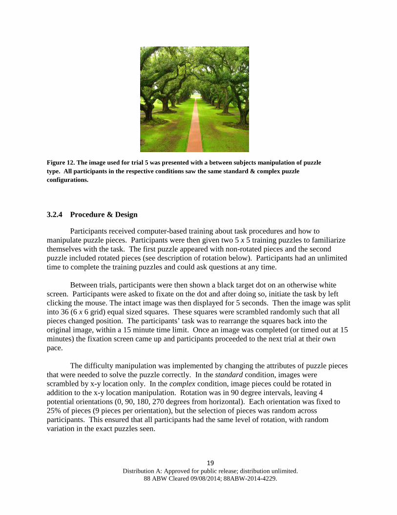
counterbalanced in pairs (see below). Figure 10 depicts image pair 1; an image of a mountain lake (left) and an image of sunflowers (right). Figure 11 depicts image pair 2; an image of the skyline of the city of Cleveland (left) and an image of an antique printing press (right). Figure 12 is the image used for the fifth trial (see below) which is an image of trees along a walkway.

Figure 10. Image pair 1 (Mountain Lake, Left; Sunflowers, Right) was always presented in trials 1 & 2 and was counterbalanced such that across participants both images were seen in standard and complex configurations and in different presentation orders.

Figure 11. Image pair 2 (Cleveland skyline, Left; Antique Printing Press, Right) was always presented in trials 3 & 4 and was counterbalanced such that across participants both images were seen in standard and complex configurations and in different presentation orders.


88 ABW Cleared 09/08/2014; 88ABW-2014-4229.

3.2.4 Procedure & Design

Participants received computer-based training about task procedures and how to manipulate puzzle pieces. Participants were then given two 5 x 5 training puzzles to familiarize themselves with the task. The first puzzle appeared with non-rotated pieces and the second puzzle included rotated pieces (see description of rotation below). Participants had an unlimited time to complete the training puzzles and could ask questions at any time.

Between trials, participants were then shown a black target dot on an otherwise white

screen. Participants were asked to fixate on the dot and after doing so, initiate the task by left clicking the mouse. The intact image was then displayed for 5 seconds. Then the image was split into 36 (6 x 6 grid) equal sized squares. These squares were scrambled randomly such that all pieces changed position. The participants’ task was to rearrange the squares back into the original image, within a 15 minute time limit. Once an image was completed (or timed out at 15 minutes) the fixation screen came up and participants proceeded to the next trial at their own pace.

The difficulty manipulation was implemented by changing the attributes of puzzle pieces

that were needed to solve the puzzle correctly. In the standard condition, images were scrambled by x-y location only. In the complex condition, image pieces could be rotated in addition to the x-y location manipulation. Rotation was in 90 degree intervals, leaving 4 potential orientations (0, 90, 180, 270 degrees from horizontal). Each orientation was fixed to 25% of pieces (9 pieces per orientation), but the selection of pieces was random across participants. This ensured that all participants had the same level of rotation, with random variation in the exact puzzles seen.

Figure 12. The image used for trial 5 was presented with a between subjects manipulation of puzzle type. All participants in the respective conditions saw the same standard & complex puzzle configurations.


88 ABW Cleared 09/08/2014; 88ABW-2014-4229.

Images were counterbalanced in pairs in which the first two trials had the same two images and the last two trials used the same images. Images were counterbalanced such that each image was seen in both standard and complex versions across participants. In all cases participants used the mouse to interact with the image, with a left click for location manipulation and a right click for rotation manipulation (when implemented).

Figure 13. A diagram of the first four experimental trials, in one of two counterbalanced configurations. Specific comparisons are annotated. The design allows for multiple comparisons of task demands, as well as practice effects.

An overview of the experimental procedure for one counterbalanced configuration, with descriptions of the task parameters is presented in

Table 1. A subset for trials 1 through 4 is diagrammed in Figure 13. The design was a

mixed design, with a within subjects manipulation of task demands. The first four trials were counterbalanced in an A-B-B-A / B-A-A-B blocked design across participants. Each A-B block was further counterbalanced across two images. This facilitated both a task demand comparison (standard to complex; trials 1 to 2 and 3 to 4) as well as multiple tests of practice in trials 1 & 4, as well as a repeated difficulty comparison in trials 2 & 3.

Table 1. An example of the experimental implementation for the first counterbalance type in Experiment 1.

Trial Number

Puzzle Type (A-B-B-A (+1) counterbalance)

Task Description

Instructions & Training (unlimited time to complete training puzzles)

Sample Standard & Complex Image

5 x 5 Randomized

Trial 1 (15 minute time limit) Standard Puzzle, Image Pair 1 6 x 6 Randomized, x-y position change

Trial 2 (15 minute time limit) Complex Puzzle Image Pair 1 6 x 6 Randomized, x-y position change + rotated pieces

Trial 3 (15 minute time limit) Complex Puzzle Image Pair 2 6 x 6 Randomized, x-y position change + rotated pieces

Trial 4 (15 minute time limit) Standard Puzzle Image Pair 2 6 x 6 Randomized, x-y position change

Standard Complex Complex Standard

Standard to Complex Comparison 1

(Task Demands)

First to Fourth Trial Comparison(Practice 2)

Standard to Complex Comparison 2(Task Demands)

Second to Third Trial Comparison (Practice 1)


88 ABW Cleared 09/08/2014; 88ABW-2014-4229.

Trial 5 (15 minute time limit) Standard or Complex Image (Between Subjects)

6 x 6 Fixed Scramble + Secondary Audio Task

The fifth trial consisted of a between subjects manipulation of standard or complex

puzzle, with the addition of a secondary audio task. There were 16 participants in the standard puzzle condition and 15 participants in the complex puzzle condition. Unlike the previous randomized puzzles, the specific order of the scramble was fixed for the final trial. One puzzle was used for both conditions (fitting with randomization parameters described above).

The secondary audio task was a radio monitoring task, in which participants were required to listen to a series of messages containing a “call sign” and a specific color/number code (e.g., Ready Tiger go to Red 7 Now). Participants responded to messages containing a specific call sign by pressing the space bar on a keyboard to activate the microphone and repeating the entire critical message. There were five distracter call signs: Arrow, Charlie, Eagle, Ringo, & Tiger. The critical call sign was Barron. There were four color coordinates (Blue, Red, White, and Green) and seven number coordinates (1 through 7), creating a pool of 28 potential critical signals among 140 possible distracter messages. All messages were 2 seconds in duration. All messages were male speakers, randomly selected from a pool of 6 possible speakers (recordings were available for all 168 possible combinations for all 6 speakers).

All participants received the same message order which was randomized according to the following parameters. Messages were presented in pairs that were programmed to overlap each other by 1 second. Beginning at 10 seconds from the start of the trial, message pairs occurred approximately every 5-6 seconds thereafter. A critical message was programmed to occur once for every 30 second time period. For the 15 minute trial, half of the critical signals were “cut ins” (the signal began in the middle of a distracter) and half were “interrupted” (the signal was interrupted by a distracter).

3.2.5 Dependent Variables

Multiple DV’s will be explored for their potential utility in distinguishing between task difficulty and time on task manipulations. Table 2 summarizes the dependent variable, description of calculation, and it’s classification of “conventional” or “dynamic” in regards to variability over time.

Table 2. Summary of dependent variables in Experiment 1. Variable Name

Description Classification

Average Fixation Time Average length of all fixations in a trial

Conventional

Fixations per Minute Number of fixations divided by Trial Time

Conventional

β Value Frequency response of Scan Path Dynamic Cross Recurrence (Piece vs. Position)

Percentage of Recurring States Dynamic

Cross Determinism (Piece vs. Position)

Percentage of Recurring States that Recur in an order

Dynamic

Diagonal Recurrence (Piece vs. Position)

Percentage of recurring states that recur at the same point in time

Dynamic


88 ABW Cleared 09/08/2014; 88ABW-2014-4229.

3.2.6 Calculation of Fixations

Fixation duration and location was determined using dispersion based techniques from Salvucci and Goldberg (2000). At a collection rate of 60 Hz, a minimum of 6 consecutively tracked points with a maximum dispersion of 1 degree (for all 6 points) was considered the minimum criterion for a fixation. The calculated centroid of the fixation points was considered the location of the fixation. The resulting location of fixation was used in conjunction with the location of the puzzle pieces to create a time series of which pieces were fixated upon, and which position on the grid that piece was in (see below). This method also yields duration for each fixation, which is then used for calculations of average fixation time.

3.2.7 Quantification of Dynamic Structure

As previously mentioned, dynamic structure in a time series can be assessed using multiple analytical tools. The present analysis will utilize two different mathematical techniques to analyze dynamic structure in eye gaze time series. The first is β values observed from angular change time series as used by Aks et al, (2002) and Stephen and Anastas (2011). The angular difference between each measured X-Y position was computed and the subsequent “gaze step” time series was then submitted to a Fast Fourier Transform variant optimized for characterizing the noise category of a time series (Eke et al, 2002).

Specifically, the Power Spectral Density Low (PSDlow) method (Eke et al, 2002) was

used to calculate the spectral slope. The first 8192 angular change values calculated for each trial were normalized to a mean of zero and a standard deviation of 1. Normalized values were then bridge detrended (a line connecting the first point and the endpoint is subtracted from the time series). The Fast Fourier Transform (FFT) was conducted on 7 data windows of 2048 data points. Four of these windows were adjoining and therefore unique (i.e. the 8192 points are divided into four adjoining sets of 2048 points), three windows overlapped the ‘borders’ of the sequential windows. The FFT values for all windows were then averaged, yielding the power spectral density profile (e.g., relative frequency to absolute power). Finally the slope was calculated on only the center of the frequency ranges (excluding the lowest 1/8 and highest 1/8 of the frequency range); this eliminates whitening of the frequency response often seen at the lowest and highest frequencies of the data (Eke et al, 2002). The resulting (log10) spectral density plot was then fit with a standard regression in which the slope is the β value.

A second technique was used to evaluate dynamic structure in the order alignment of

piece and position fixations. As previously mentioned, Cross Recurrence Quantification Analysis (CRQA) provides multiple dependent variables which quantify the level and types of dynamic structure seen between two time series (Webber and Zilbut, 2005; Dale et al, 2011). This type of analysis was instantiated for nominal or categorical time series in accordance with practices from Richardson & Dale (2005). In the present analysis, two categorical time series of fixations were generated: A time series of the positions of the board and a time series of the pieces of the puzzle that were the focus of the fixation. Each time series was windowed in increments of 400 fixations; for CREC and CDET the average values across windows were used


88 ABW Cleared 09/08/2014; 88ABW-2014-4229.

for subsequent inferential analysis. Subsequent to the initial CRQA analysis, diagonal recurrence profiles were calculated across the entire time series in accordance with Richardson and Dale (2005) to determine the coupling observed between position and piece of fixation.

In order to determine whether or not any dynamic structure observed is a product of

chance, all dynamic structure analyses were subjected to surrogation tests. Time series were randomly shuffled and re-analyzed. In the surrogated analyses, any significant temporal structure present in the original time series should be lost, e.g., β values should approach zero, %CREC & %CDET should approach chance levels. In all cases for all dynamic variables, the surrogated measures’ values were statistically different from measures calculated from the original time series, as measured by paired samples t-tests (p >. 05).

3.3 Results

3.3.1 Results for Trials 1 through 4

For trials 1 to 4, all dependent variables were subjected to a 2 x 2 x 2 mixed ANOVA with 2 levels of task demands (within subjects factor of standard or complex puzzle), 2 levels of practice (within subjects factor of first presentation or second presentation) and 2 levels of counterbalance (between subjects presentation order of Standard-Complex-Complex-Standard (SCCS) or Complex-Standard-Standard-Complex (CSSC)). Aside from completion time, which had a directional expectation, the statistical tests for Experiment 1 were explicitly two tailed.

Completion time had a significant main effect of task demands such that complex puzzles

took longer to complete than standard puzzles as shown in

Table 3. There was no indication of a performance difference with practice (i.e. no difference between presentations 1 & 2), nor were any other main effects or interactions significant for completion time. The differences in completion time were also reflected in the ability of participants to solve the puzzles in the allotted time. For standard puzzles, 57 of 62 puzzles were successfully solved (92%), with 5 of 62 (8%) puzzles unsolved. For complex puzzles 29 of 62 puzzles (47%) were successfully solved, and 33 of 62 puzzles (53%) unsolved. Separate 2 x 4 chi squared analyses (one for each difficulty) were performed to address any potential differences in solve rates between the four images used. In both cases there were no significant differences in solve rates between images: Standard puzzles χ2(3) = .58, p > .05.; Complex puzzles χ2(3) = 6.94, p > .05. Taken together, these results confirm the expectation that complex puzzles were more difficult when compared to standard puzzles, and that difficulty differences were driven by the puzzle type manipulation and not aspects any individual image.

Conventional gaze metrics included in the present analysis were fixations per minute and

average fixation length. There was a main effect of task demands for fixations per minute, as shown in

Table 3. The number of fixations per minute was lower for complex puzzles than for standard puzzles. Average fixation length exhibited a significant main effect of task demands, as shown in


88 ABW Cleared 09/08/2014; 88ABW-2014-4229.

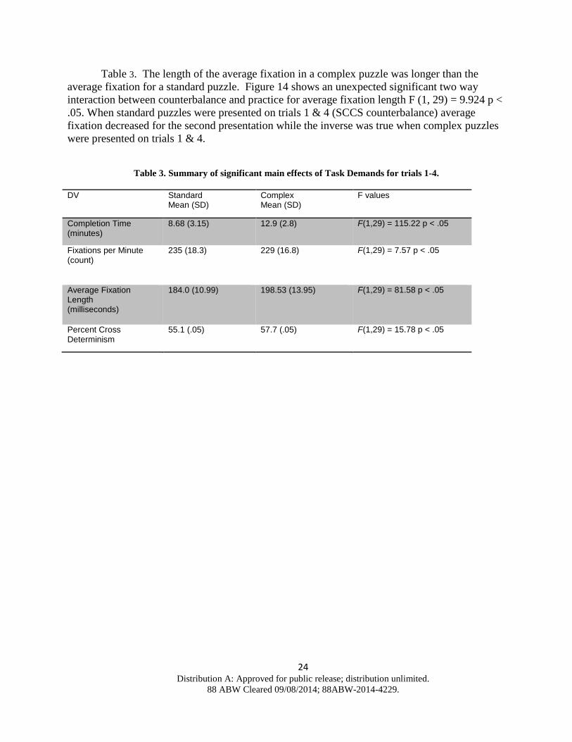
Table 3. The length of the average fixation in a complex puzzle was longer than the average fixation for a standard puzzle. Figure 14 shows an unexpected significant two way interaction between counterbalance and practice for average fixation length F (1, 29) = 9.924 p < .05. When standard puzzles were presented on trials 1 & 4 (SCCS counterbalance) average fixation decreased for the second presentation while the inverse was true when complex puzzles were presented on trials 1 & 4.

Table 3. Summary of significant main effects of Task Demands for trials 1-4.

DV Standard Mean (SD)

Complex Mean (SD)

F values

Completion Time (minutes)

8.68 (3.15) 12.9 (2.8) F(1,29) = 115.22 p < .05

Fixations per Minute (count)

235 (18.3) 229 (16.8) F(1,29) = 7.57 p < .05

Average Fixation Length (milliseconds)

184.0 (10.99) 198.53 (13.95) F(1,29) = 81.58 p < .05

Percent Cross Determinism

55.1 (.05) 57.7 (.05) F(1,29) = 15.78 p < .05


88 ABW Cleared 09/08/2014; 88ABW-2014-4229.

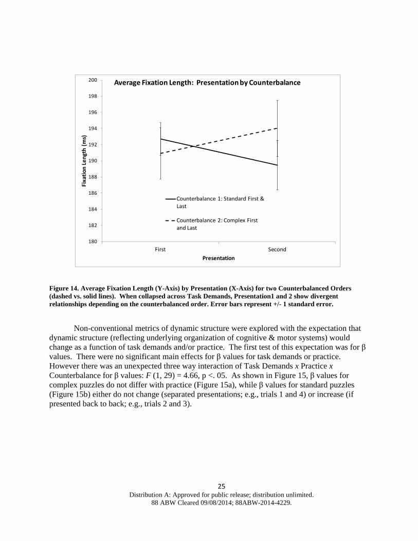
Figure 14. Average Fixation Length (Y-Axis) by Presentation (X-Axis) for two Counterbalanced Orders (dashed vs. solid lines). When collapsed across Task Demands, Presentation1 and 2 show divergent relationships depending on the counterbalanced order. Error bars represent +/- 1 standard error.

Non-conventional metrics of dynamic structure were explored with the expectation that dynamic structure (reflecting underlying organization of cognitive & motor systems) would change as a function of task demands and/or practice. The first test of this expectation was for β values. There were no significant main effects for β values for task demands or practice. However there was an unexpected three way interaction of Task Demands x Practice x Counterbalance for β values: F (1, 29) = 4.66, p <. 05. As shown in Figure 15, β values for complex puzzles do not differ with practice (Figure 15a), while β values for standard puzzles (Figure 15b) either do not change (separated presentations; e.g., trials 1 and 4) or increase (if presented back to back; e.g., trials 2 and 3).

180

182

184

186

188

190

192

194

196

198

200

First Second

Fixa

tion

Leng

th (m

s)

Presentation

Average Fixation Length: Presentation by Counterbalance

Counterbalance 1: Standard First & Last

Counterbalance 2: Complex First and Last


88 ABW Cleared 09/08/2014; 88ABW-2014-4229.

a.) b.)

Figure 15. a.) β values (Y-Axis) by presentation (X-Axis) for Complex puzzles in two Counterbalanced Orders (dotted vs. solid lines). β values did not change across presentations or differ based on the order of the counterbalance. Error bars represent +/- 1 standard error. b.) β values (Y-Axis) by Presentation (X-Axis) for Standard puzzles in two Counterbalanced Orders (dashed vs. solid lines). When the two presentations were separated (solid line) β values were unchanged, however when the two presentation occurred back to back β values increase from Presentation 1 to Presentation 2. Error bars represent +/- 1 standard error.

In addition to frequency-based measures, metrics of dynamic structure derived from a cross recurrence matrix of piece and position of fixation were tested. For the most basic of these, cross recurrence, there were no significant main effects or interactions. However, cross determinism had a significant main effect of task demands (

Table 3) and practice (Table 4). Cross determinism increases by around 2% for both Complex Puzzles (vs. Standard) and the Second Presentation (vs. First).

There was a significant effect of practice for diagonal recurrence as shown in Table 4.

Diagonal recurrence increases by around 4% from the first to the second presentation. In this context, diagonal recurrence represents an increase in fixations upon pieces that are in the correct positions. Note that this explicit relationship between piece and position is due to the measurement of diagonal recurrence at zero lag.

Table 4. Summary of significant main effects of Practice for trials 1-4.

DV First Presentation Mean (SD)

Second Presentation Mean (SD)

F values

Diagonal Recurrence Profile

18.9 (10.4) 23.2 (11.9) F(1,29) = 4.66 p < .05


55.6 (.05) 57.2 (.04) F(1,29) = 5.99 p < .05

-1.4

-1.35

-1.3

-1.25

-1.2

-1.15

-1.1

First Presentation Second Presentation

B Values: Counterbalance by Trial for Complex Puzzles

Complex Trials 2 & 3

Complex Trials 1 & 4

-1.4

-1.35

-1.3

-1.25

-1.2

-1.15

-1.1

First Presentation Second Presentation

B Values: Counterbalance by Trial for Standard Puzzles

Standard Trials 1 & 4

Standard Trials 2 & 3


88 ABW Cleared 09/08/2014; 88ABW-2014-4229.

3.3.2 Results for Trial 5

For the inferential analysis of the final trial, which included a secondary audio task, the dependent variables were subjected to a one-way between-subjects ANOVA for Task Demands (Standard vs. Complex). The significant results can be seen in Table 5. The general expectation for Trial 5 was that secondary task performance would not change, but the addition of a secondary task could alter puzzle performance and/or gaze behavior by reducing spare capacity of the participants.

For the primary task of solving the puzzle, there was a main effect of Completion Time,

as shown in Table 5. As expected, the Complex puzzle took longer to complete than the Standard puzzle. This was consistent with the results for trials 1-4.

The secondary audio task was scored for accuracy of responses to critical signals. The

values were percentages, since the number of critical signals heard by the participant was determined by their performance time. As expected, there were no significant differences in the percentage of correct signals between levels of Task Demands. The mean percentage for Standard puzzles was 85.6% correct with a standard deviation of 27%. For Complex puzzles the mean was 82.5% correct with a standard deviation of 29.9%.

Average Fixation Length had a significant relationship with Task Demands, with

Complex puzzles exhibiting an average length approximately 14 ms longer than Standard puzzles. This was the same direction as was seen in trials 1-4.

β values did not differ for different Task Demands. The average β for Standard puzzles

was -1.29 (SD = .13) and was -1.31 (SD = .13) for Complex puzzles. This did not support the expectation that β values would be sensitive to changes in task demands.

Recurrence-based metrics show a significant increase in Percent Cross Recurrence as

well as Percent Cross Determinism. Cross Recurrence was 1.1% higher for Complex Puzzles as compared to standard puzzles, and Cross Determinism was 8% higher for Complex Puzzles. Diagonal Recurrence was not different across Task Demands. These results support the expectation of a change in dynamic structure under different Task Demands. Cross Recurrence and Cross Determinism both indicate increasing structure with higher task demands, similar to what was observed for trials 1-4.

Table 5. Summary of significant results for Trial 5. DV Standard

Mean (SD) Complex Mean (SD)

F values

Completion Time (minutes)

6.89 (2.88) 11.19 (2.89) F(1,29) = 115.22 p < .05


192.69 (12.05) 206.66 (10.77) F(1,29) = 11.52 p < .05


88 ABW Cleared 09/08/2014; 88ABW-2014-4229.

Percent Cross Recurrence

4.2 (.64) 5.3 (1.2) F(1,29) = 9.6 p < .05


55.16 (6.3) 63.0 (3.7) F(1,29) = 17.35 p < .05

In order to determine the impact of the secondary audio task completion time, an analysis

was conducted which compared completion time for Trial 5 to the second presentation (i.e., Trial 3 or 4) of the corresponding difficulty condition to that presented in Trial 5. The main effects of this analysis are presented in Table 6. Overall, the secondary task shows very little impact; there was no difference in completion time between the paired trials. The only significant differences point to effects of Practice, similar to what was observed for trials 1-4.

Table 6. Summary of significant main effects for paired difficulty comparisons with and without the secondary task.

DV Presentation 2 Mean (SD)

Trial 5 Mean (SD)

F values

Diagonal Recurrence (percent)

22.04 (12.5) 35.09 (13.07) F(1,27) = 15.976 p < .05


191.6 (11.77) 199.4 (13.31) F(1,27) = 39.714 p < .05

3.4 Discussion

At the outset of Experiment 1, it was hypothesized that the manipulation of Task Demands would cause a change in Completion Time; the primary question was if eye gaze measures would be sensitive to the changes, and furthermore if a distinction occurred between the types of eye gaze measures (conventional and dynamic). This question was also presented in regards to Time on Task, as well as spare capacity (Trial 5). The manipulation of Task Demands had the expected effect on Completion Time, which was an important manipulation check. The findings of Experiment 1 supported the expectation that eye gaze would reflect differences in Completion Time.

Previous work suggested that the addition of secondary task might change gaze behavior

(e.g., May et al, 1990), however the data from Trial 5 seems to suggest that there were no significant impacts of spare capacity on gaze behavior. When the eye gaze measures from Trial 5 were compared to the corresponding puzzle type from the second presentation (i.e. Trial 3 or Trial 4 depending on the counterbalance) the trends observed in trials 1-4 are unchanged when participants completed a radio monitoring task while completing the puzzle. This may be due to different resources required for both tasks, (i.e., visual vs. auditory; Wickens, 2002). This would create a situation in which the two types of tasks used here would be least likely to impact one


88 ABW Cleared 09/08/2014; 88ABW-2014-4229.

another. However, two different task types were required so that the visual display would be unchanged with the addition of the secondary task.

Generally, measures of eye gaze were sensitive to the different puzzle types. However

there was no clear distinction between conventional and dynamic measures of gaze; measures of averaged fixation activity and recurrence measures both showed significant effects of Task Demands. Average Fixation Length (with a corresponding decrease in Fixations per Minute) and Cross Determinism were both higher in Complex puzzles. In the present context, Cross Determinism represents a relationship between piece and position of fixation that is consistent in time, although not necessarily the correct piece/position placement. Taken together, there was a tendency to fixate for longer periods of time (and a fewer number of times) in a more structured sequence in Complex Puzzles. Longer fixations are likely due to the time it takes to orient pieces when rotated. Deterministic sequences of fixations suggest there is an increase in repeated fixations for pieces in the same piece/position configuration for complex puzzles. This likely reflects looking from one piece to another and then back in order to determine where/if the piece should be moved.

In regards to practice or learning effects, it was expected that learning or strategy shifts

could be seen in Completion Time and also reflected in gaze patterns at different presentations. While there were no changes in Completion Time, there were main effects of Practice for the recurrence-based metrics of Percent Cross Determinism and Diagonal Recurrence. In this case, it’s likely that the increase in Percent Determinism is directly related to the increase in Diagonal Recurrence; Determinism quantifies all sequential fixations, and Diagonal Recurrence quantifies a subset of those sequential fixations, specifically those in which piece and position are exact matches in time. As previously mentioned, the increase in Diagonal Recurrence suggests that participants are learning about the task; they are increasing the number of fixations on pieces in the correct positions. In terms of looking at the images, it could be the case that participants were using pieces that had been correctly placed as references or anchors from which to select and place other pieces. However, there was no effect of Completion Time for Practice, so this change in gaze patterns did not result in a faster performance outcome.

While only dynamic measures showed significant main effects, Average Fixation Length

had an interaction with Time on Task and Counterbalance, suggesting that the order of the puzzle presentations had an effect on the length of fixation. Specifically, the two counterbalance types show a divergent relationship. Participants in the SCCS counterbalance show an increase in fixation lengths from the first to the second presentation, whereas those in the CSSC counterbalance shows decreasing fixation lengths on the second presentation. It would only be speculative to interpret this finding, other than to interpret some form of transfer in gaze strategy that is different between the two presentation orders.

It was expected that the frequency patterns in the scan path, as measured by β values,

would be classified as 1/f patterns, as has been reported in previous work (Aks et al, 2002 and Stephen & Anastas, 2011), and this was the case. It was further expected that β values would be sensitive to changes in task demands, based partially on the results from Stephen and Anastas (2011) which link increases in β values to faster reaction times. However, β values did not


88 ABW Cleared 09/08/2014; 88ABW-2014-4229.

change with Task Demands, or at least not in a straightforward manner. Rather than respond to Task Demands alone, β values for Experiment 1 suggest some type of transfer of gaze patterns between the two presentations that is dependent on which type of puzzle was seen first. At this point there is not an explanation for this pattern and it would be extremely speculative to interpret further.

4.0 EXPERIMENT 2

4.1 Introduction

Overall, the results from Experiment 1 provide mixed answers for the research questions of interest at the outset. On one hand, eye gaze metrics were sensitive to the manipulation of task demands, a demonstration of the link between gaze behavior and performance outcomes. On the other hand, this was the case for both types of eye gaze metrics (conventional and dynamic). Expanding the view to the Practice measures, there is an indication that the dynamic measures may be sensitive to a shift in gaze strategy in ways that conventional measures of eye gaze are not, but this distinction should be given further study since there was an interaction with counterbalance type. It was unexpected that the counterbalance type would show significance in the inferential tests; the counterbalancing of an experimental design is undertaken to nullify interactions between manipulations. The interactions suggest that the changes over time that may be due to practice or learning may have been interrupted by the manipulation of task demands in some way that is unclear at this time.

In an attempt to better understand changes of gaze strategy with Practice, a short (e.g.,

pilot), follow-up experiment was conducted which did not include manipulations of Task Demands. Experiment 2 was a test of repeated presentations of the same image and puzzle type. The expectation was that Completion Time would improve with repeated presentations of the same puzzle/image combination. The goal of the Experiment 2 was to initiate systematic learning improvements in participants’ completion times, and to determine the degree to which these changes are reflected in different measures of eye gaze (e.g., Average Fixation Length, β values, and Diagonal Recurrence).

4.2 Methods

4.2.1 Participants

All participants in Experiment 2 had successfully completed Experiment 1 (see above for requirements). Although 6 participants were initially tested, one participant’s data was excluded due to a calibration error, resulting in data from 5 participants being included in the analysis for Experiment 2.

4.2.2 Image Selection

Two images were selected for Experiment 2; both images had previously been included in either the image selection process or in data collection for Experiment 1. One image, a sport utility vehicle (Figure 16, left) was used from the pilot image selection process in Experiment 1.


88 ABW Cleared 09/08/2014; 88ABW-2014-4229.

Another image (Figure 16, right) was re-used from Experiment 1, the image of sunflowers. Images were randomly assigned to participants.

Figure 16. The two images used between subjects in Experiment 2. The Vehicle (left image) was used in the pilot testing of Experiment 1; the Sunflowers (right image) image was used for data collection in Experiment 1.

4.2.3 Apparatus

Workstation and eye tracking apparatus were the same as those used for Experiment 1. Eye tracking was conducted via a Facelab4 “off the head” eye tracker, hosted on a Dell Latitude D830 laptop computer (2.2 GHz processor, 2 GB RAM). This combination allows for +/- 1 degree of visual angle eye tracking capability at a collection rate of 60Hz. Facelab API version 4.6 was integrated with custom software written to display images for this experiment. The output of the tracking software was the X and Y pixel location of participants’ gaze.

The participant station was an HP Compaq DC80 desktop computer (2.3 GHz processor, 3.5 GB RAM) & a LCD monitor (Samsung 940BX) with a height of 30 cm and a width of 37.5cm (48cm diagonal), at 1280 x 1024 resolution.

Images were sized at 1020 x 1020 pixels, and at a viewing distance of approximately 60cm, which is approximately 27 x 27 degrees of visual angle. When subdivided for the puzzle into 36 equal sized square pieces (170 pixels width/height), each piece was approximately 4.75 x 4.75 degrees of visual angle.

4.2.4 Procedure and Design

Participants were given verbal instructions about the task procedures and how to manipulate the puzzle pieces. Following instructions, participants completed one 5 x 5 practice image to familiarize themselves with the task. Once participants solved the practice image, participants were presented a series of 9 trials of the same test image in the rotated condition.


88 ABW Cleared 09/08/2014; 88ABW-2014-4229.

Rotation was in 90 degree intervals, leaving 4 potential orientations (0, 90, 180, 270 degrees from horizontal). Each orientation was fixed to 25% of pieces (9 pieces per orientation). Between trials, participants were shown a black target dot on an otherwise white screen. Participants were asked to fixate on the dot and after doing so, initiate the task by clicking the left mouse button. The intact image was then displayed for 5 seconds. Then the image was split into 36 (6 x 6 grid) equal sized squares. The puzzles were generated in a randomized way such that all pieces changed position. Each trial lasted until the participant completed the puzzle; there were no time limits in Experiment 2.

4.3 Results

In Experiment 2 all dependent variables were subjected to a one-way ANOVA for trial to explore potential relations to experience or learning. It was expected that overall performance would improve over trials (i.e., Completion Time would decrease). A primary question was the degree to which conventional measures of eye gaze (Average Fixation Length or Fixations per Minute) and/or alternative measures derived from dynamical systems theory (β, Cross Recurrence, Cross Determinism, and Diagonal Recurrence) would provide additional insights into the performance changes.

As shown in Figure 17, the expectation that Completion Time would decrease was supported; there was an overall effect of trial on Completion Time, as reported in Table 7. This change was in the expected direction: Average Completion Time was reduced from 10.19 min on Trial 1 to 2.87 min on Trial 9. Completion time sharply decreased after Trial 1, asymptoting around Trial 5.

For all hypothesized effects, regression models were fit to the data to determine the type

of trend observed. Three model fits were chosen based on research in the domain of nonlinear dynamics and learning (Crites and Gorman, 2013): linear, exponential, and power law. As a first step, linear should be tested at it is the simplest model fit. Both exponential and power were fit in order to discriminate between two; different types or categories of learning (Crites and Gorman, 2013). Exponential models are associated with learning novel skills, while power law fits are associated with persistent learning (e.g., tuning or refining existing skills) (Stratton et al., 2007). The R squared values for the model fits are summarized in Table 8. The trajectory for Completion Time was best fit by a power law, which had a better fit than the exponential & linear models (Table 8). Taken together, there is strong evidence that learning was taking place with repeated exposure to puzzles of the same image.


88 ABW Cleared 09/08/2014; 88ABW-2014-4229.

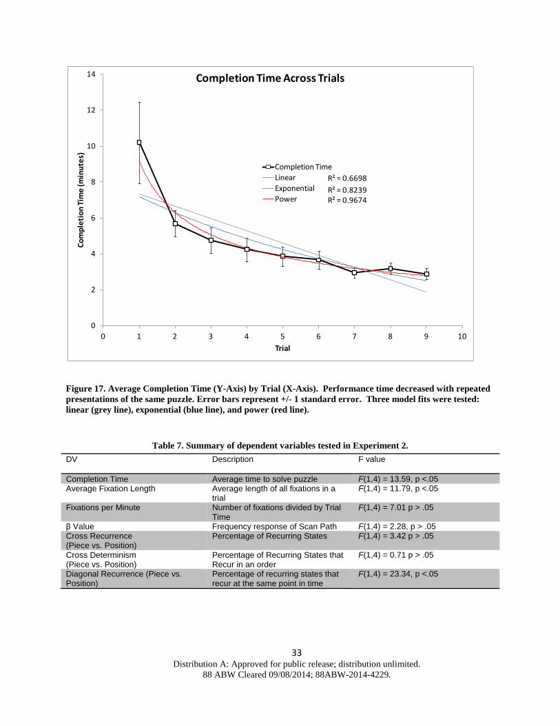
Figure 17. Average Completion Time (Y-Axis) by Trial (X-Axis). Performance time decreased with repeated presentations of the same puzzle. Error bars represent +/- 1 standard error. Three model fits were tested: linear (grey line), exponential (blue line), and power (red line).

Table 7. Summary of dependent variables tested in Experiment 2. DV

Description F value

Completion Time Average time to solve puzzle F(1,4) = 13.59, p <.05 Average Fixation Length Average length of all fixations in a

trial F(1,4) = 11.79, p <.05

Fixations per Minute Number of fixations divided by Trial Time

F(1,4) = 7.01 p > .05

β Value Frequency response of Scan Path F(1,4) = 2.28, p > .05 Cross Recurrence (Piece vs. Position)

Percentage of Recurring States F(1,4) = 3.42 p > .05

Cross Determinism (Piece vs. Position)

Percentage of Recurring States that Recur in an order

F(1,4) = 0.71 p > .05

Diagonal Recurrence (Piece vs. Position)

Percentage of recurring states that recur at the same point in time

F(1,4) = 23.34, p <.05

R² = 0.6698R² = 0.8239R² = 0.9674

0

2

4

6

8

10

12

14

0 1 2 3 4 5 6 7 8 9 10

Com

plet

ion

Tim

e (m

inut

es)

Trial

Completion Time Across Trials

Completion TimeLinearExponentialPower


88 ABW Cleared 09/08/2014; 88ABW-2014-4229.

Table 8. Summary of model fits for the hypothesized effects in Experiment 2. DV Linear R2 Exponential R2 Power R2 Completion time .67 .82 .97 Average fixation length

.25 .26 .51

Diagonal recurrence

.67 .59 .81

β Value .57 .58 .59 For conventional eye gaze metrics, it was expected that there would be a significant

relationship between Trial and Average Fixation Length in Experiment 2. This expectation was based on the significant two way interaction (Practice x Counterbalance) for Average Fixation Length that was observed in Experiment 1. This expectation was supported: Average Fixation Length increased over the first 5 trials and then seemed to level off at about 200 ms in the final 4 trials as shown in Figure 18. There was a significant effect of Trial for Average Fixation Length, as shown in Table 7. When compared to Completion Time, as trial length decreased the length of the fixations increased. When fit with regression models, Average Fixation Length (Figure 18; Table 8) shows a moderate power law relationship. Taken together, this indicates that while Average Fixation Length changes over the course of 9 trials, it is not necessarily changing systematically with Completion Time.


88 ABW Cleared 09/08/2014; 88ABW-2014-4229.

Figure 18. Average Fixation Length (Y-Axis) by Trial (X-Axis). Average fixation length increased as a function of trial. Error bars represent +/- 1 standard error. Three model fits were tested: linear (grey line), exponential (blue line), and power (red line).

β values were tested for change as a function of Trial, in an attempt to clarify relationships observed in Experiment 1. There was not a significant change in β values with learning, as shown in Table 7. Figure 19 depicts the absolute value of β values across 9 trials. Absolute values are plotted (rather than the original negative slope values) in order to model the data (power law fit cannot be computed for negative values). As shown in Figure 19, β values are generally flat with an absolute mean value across trials of 1.14 (signed value is -1.14). β values in this range are representative of 1/f noise, suggesting that ‘optimum’ dynamic structure is present in the scan path, but this measure of structure does not change as a function of learning in this task. Regression fits for β values (Figure 19; Table 8) show that all models fit the data moderately well (e.g., ~ .57 R2 with no distinctions among the three). Overall, this suggests that β Values are not diagnostic in terms of learning or strategy for this task.

R² = 0.2548

R² = 0.2625

R² = 0.5039

150

160

170

180

190

200

210

220

230

0 1 2 3 4 5 6 7 8 9 10

Fixa

tion

Leng

th (m

s)

Trial

Average Fixation Length Across Trials

Avg. Fix. Length

Linear

Exponential

Power


88 ABW Cleared 09/08/2014; 88ABW-2014-4229.

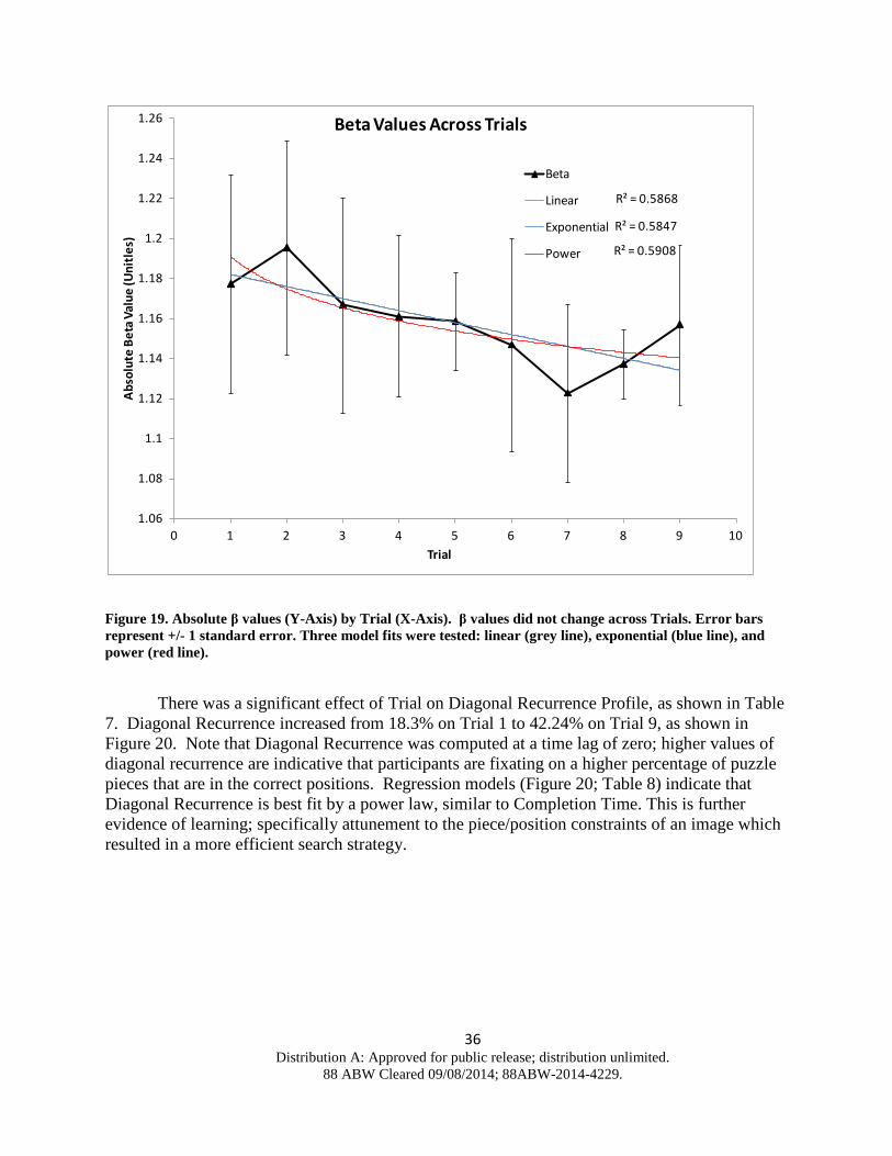
Figure 19. Absolute β values (Y-Axis) by Trial (X-Axis). β values did not change across Trials. Error bars represent +/- 1 standard error. Three model fits were tested: linear (grey line), exponential (blue line), and power (red line).

There was a significant effect of Trial on Diagonal Recurrence Profile, as shown in Table 7. Diagonal Recurrence increased from 18.3% on Trial 1 to 42.24% on Trial 9, as shown in Figure 20. Note that Diagonal Recurrence was computed at a time lag of zero; higher values of diagonal recurrence are indicative that participants are fixating on a higher percentage of puzzle pieces that are in the correct positions. Regression models (Figure 20; Table 8) indicate that Diagonal Recurrence is best fit by a power law, similar to Completion Time. This is further evidence of learning; specifically attunement to the piece/position constraints of an image which resulted in a more efficient search strategy.

R² = 0.5868

R² = 0.5847

R² = 0.5908

1.06

1.08

1.1

1.12

1.14

1.16

1.18

1.2

1.22

1.24

1.26

0 1 2 3 4 5 6 7 8 9 10

Abso

lute

Bet

a Val

ue (U

nitle

s)

Trial

Beta Values Across Trials

Beta

Linear

Exponential

Power


88 ABW Cleared 09/08/2014; 88ABW-2014-4229.

Figure 20. Percent Diagonal Recurrence (Y-Axis) by Trial (X-Axis). Diagonal Recurrence increases with repeated puzzle presentations. Error bars represent +/- 1 standard error. Three model fits were tested: linear (grey line), exponential (blue line), and power (red line).

The results for the analyses of variance in Experiment 2 indicate that there was a significant drop in Completion Time, and that there were significant effects of Trial for two of the eye gaze metrics (Average Fixation Length, Diagonal Recurrence). The model fits give some insight to relationships between the gaze measures and Completion Time. However, to further quantify the relationships between eye gaze metrics and Completion Time, a correlation analysis was performed.

The repeated measures design means that an omnibus correlation analysis (all

participants and all trials in the same test) would be inappropriate. To estimate the correlation across participants, correlations were computed for each participant and averaged in accordance with the procedures provided in Silver and Dunlap (1987). Briefly, for each participant, a Pearson’s correlation between all eye gaze metrics and completion time was computed across trials. The computed r values were converted to Fisher’s z values and averaged across participants. The averaged z scores were then re-converted to Pearson r values and tested for significance. This procedure is necessary due to the low sample size for Experiment 2, and bias

R² = 0.67

R² = 0.5888

R² = 0.8106

0

10

20

30

40

50

60

0 1 2 3 4 5 6 7 8 9 10

Diag

onal

Rec

urre

nce

(Per

cent

)

Trial

Diagonal Recurrence Across Trials

Diagonal RecurrenceLinear

Exponential

Power


88 ABW Cleared 09/08/2014; 88ABW-2014-4229.

in the r statistic present at higher values that make it unsuitable to average the raw scores (Silver & Dunlap, 1987). The average r values can be seen in Table 9.

Given the low number of subjects for Experiment 2, an alpha of .1 was used for significance testing of correlations. At the .1 level, Diagonal Recurrence had a strong negative correlation with performance time, r (3) = -.85, p < .10. The correlation results (Table 9) along with the model fits (e.g., Figure 20, Table 8) indicate that Diagonal Recurrence had the strongest relationship with Completion Time. Furthermore, Diagonal Recurrence provides complimentary information above and beyond other metrics: Specifically, better puzzle performance (lower Completion Time) is seen when search behavior is more efficient (higher Diagonal Recurrence).

Table 9. Average correlation coefficients for the dependent variables tested in Experiment 2.

DV Completion time

β value

Diagonal recurrence

Cross recurrence

Cross determinism

Average fixation length

Fixations per minute

Completion time --- -0.27 -0.85* 0.31 -0.07 -0.66 0.45

β value --- 0.26 0.0 -0.05 0.2 -0.2

Diagonal recurrence --- -0.08 0.12 0.62 -0.46

Cross recurrence --- 0.4 -0.07 0.14

Cross determinism --- 0.15 0.33

Average fixation length --- -0.61

Fixations per minute ---

Note: *p<.1, critical r = .805

No other correlations between eye gaze metrics or completion time were significant at the .1 level. Although there was a significant result in the ANOVA, the moderate correlation between Average Fixation Length and Completion Time was not significant. These results should include the caveat that because of the small sample size in Experiment 2, this correlation might reach statistical significance with a larger sample. At the outset of Experiment 2, β was hypothesized to be related to Completion Time. However, based on the outcome of the ANOVA as well as the regression model fits, it is not surprising that β values are uncorrelated with Completion Time. This suggests that while there are 1/f dynamics exhibited in the scan path for this task, those dynamics are relatively stable and do not change, even as structure increases for fixations, specifically Diagonal Recurrence. This could be interpreted as anchoring and


88 ABW Cleared 09/08/2014; 88ABW-2014-4229.

efficiency; much like a traditional puzzle in which one seeks out the important pieces for the puzzle (in a typical puzzle the “edge” pieces), in this task participants were likely seeking distinctive pieces of the puzzle. For early trials, these pieces are not in the correct positions, but still provide an anchor from which to seek other matching pieces (e.g., structure in the scan path). With multiple iterations of the puzzle, learning takes place. The overall strategy is the same (seeking anchors) but with learning more of the pieces are placed in the correct positions earlier in the trial.

5.0 GENERAL DISCUSSION

The present work was undertaken to explore the possibility of eye gaze as a primary measure for state assessment by using alternative indices of dynamic structure. It was expected that eye gaze would be related to performance, but at the outset, it was not known the direction of the corresponding shift that might be seen in the dynamic patterns of eye gaze. Also of interest was the degree to which measures of dynamic structure would correspond to more conventional measures of eye gaze. Although the general expectations were addressed previously, further interpretation of the results will be organized around the general effects of Task Demands and Learning, along with general conclusions and future directions.

5.1 Task Demands & Gaze Patterns

At the outset of Experiment 1, a primary question of interest was the degree to which changes in the difficulty of the task, (standard vs. rotated puzzles) would influence performance outcomes, and if corresponding changes would also be reflected in gaze patterns. The expectation for performance changes was supported by the data as complex puzzles took longer to complete than standard puzzles. Essentially, the information (degrees of freedom) for each piece was increased when some of the pieces were rotated in the complex puzzle condition and this is reflected in the increased performance time. This result was not surprising; however it was an important manipulation check.

It was expected that changes in puzzle type would influence eye gaze metrics; and the expectation that eye gaze would be sensitive to difficulty changes in this task was supported. A second question concerned any potential differences between conventional and dynamic measures. There was no distinction between conventional and dynamic measures in regards to task difficulty; both types showed significant effects. Average fixation length was higher in complex puzzles, likely due to the need to fixate longer while pieces are rotated to their correct orientations. Higher levels of determinism in complex puzzles could indicate an anchoring strategy, as previously mentioned.

The expectation that spare capacity of the participants would alter gaze patterns was not supported. When completing the secondary audio task, participants’ task performance and gaze patterns did not change in a measureable way. There was a generally detectable difference between levels of Task Demands for Completion Time and Average Fixation Length, but no interactions or differences when compared to puzzles of the same type from trials 1-4. Comparison of matched puzzle conditions with and without the secondary task showed no difference in performance; and gaze patterns showed similar effects to trials 1-4.


88 ABW Cleared 09/08/2014; 88ABW-2014-4229.

It may be the case that the type of task, as well as the manipulation of task demands implemented in Experiment 1 were not robust enough to alter gaze patterns in a way that dynamic measures would be differentially sensitive. The literature regards 1/f as a relatively stable phenomenon; deviations occur when systems are in a state of pathology or other significant duress that deviations are seen (Bassingthwaighte, 1994). Although there was not an expected distinction between conventional and dynamic measures of gaze, there was support for the idea that gaze patterns reflect changes in Task Demands. The current results lend support to the use of eye gaze as a measure of task difficulty for the purposes of state assessment in the task used. However, eye gaze also appeared to be related to a different aspect of performance, specifically learning and strategy.

5.2 Learning & Gaze Patterns

There was support for the idea that gaze patterns would change as a result of learning. Learning effects were more nuanced than the results for Task Demands. In Experiment 1, there were significant interactions of Average Fixation Length and β values involving the counterbalance in the first experiment that are difficult to interpret, other than suggesting that there was a transfer of gaze strategy that was different depending on the order of puzzle type; and that trials 2 & 3 (repeating puzzle types) show different relationships than trials 1 & 4 (separated presentations of the same puzzle type). Addressing this issue was a primary motivation for Experiment 2, which showed a clear performance improvement as participants learned the particular aspects of each image. Experiment 2 also provided insight into which gaze measures were sensitive to learning effects.

Average Fixation Length had significant relationships with trial in both experiments; however the data from Experiment 2 suggest that over time an increase in the average fixation length occurs. There are multiple reasons why this could be the case; it is difficult to discriminate with the present results. In Experiment 2 all trials included complex puzzles; the increase in fixation time could be the result of more time spent studying individual pieces. It could also be the result of learning the general features of individual pieces and making one fixation that allowed participants to “see” multiple pieces (i.e. attend to different areas within the visual field; Heinen et al., 2011).

Data from Experiment 2 suggest that β values did not change significantly with learning; however they were in the range of 1/f phenomena. This suggests that the scan path within each trial is characterized by a relatively stable power law (as stated previously 1/f frequency responses are indicative of power law relationships). As previously stated, power law relationships are representative of tuning or refining existing learning, rather than learning new skills (Crites and Gorman, 2013). It’s easy to see why visual search would fit these criteria; from early ages we are searching for objects in the environment, and the present task is a different spin on visual search. The power law finding is consistent with research from Aks (2011), who determined 1/f patterns were present in visual search. Both Aks et al. (2011) and Stephen and Anastas (2011) interpret 1/f patterns as efficient search. The current data supports this idea; but provides further evidence via the cross recurrence based measure of diagonal recurrence.


88 ABW Cleared 09/08/2014; 88ABW-2014-4229.

http://olc1.ohiolink.edu/search%7ES0*eng?/aBassingthwaighte%2C+James+B./abassingthwaighte+james+b/-3,-1,0,B/browse

In Experiment 1, a main effect of trial was observed for Diagonal Recurrence, which was higher for the second presentation of a puzzle. This was interpreted as learning a more efficient search strategy. This is because Diagonal Recurrence represents a specific type of structure in the pattern of fixations, specifically more fixations upon puzzle pieces in their correct positions. Note that for Experiment 1, the images seen in presentations 1 and 2 were counterbalanced; suggesting that participants’ strategy shift is not due to properties of a particular image. This suggests that gaze strategy as measured by diagonal recurrence may precede performance changes in some cases.

When repeating puzzles containing the same image, as in Experiment 2, the learning effect becomes more pronounced in gaze patterns, specifically those patterns measured by Diagonal Recurrence. As properties of a specific image become apparent, a more efficient gaze strategy in which participants anchor their search on pieces in the correct positions results. Although there were significant effects for both conventional and dynamic measures of eye gaze, Experiment 2 has limited support for the idea that dynamic measures are more sensitive to changes in performance due to learning or strategy, since Diagonal Recurrence had the highest correlation with performance.

5.3 General Conclusions & Future Directions

Diagonal Recurrence was likely related to better task performance by learning a more efficient search strategy. If this is the case, then differences in Diagonal Recurrence should be seen between participants who did and did not solve a puzzle. A subset of the data from Experiment 1, specifically the 2nd presentation of the complex puzzle, was selected as a test of this idea. From this subset, 13 participants solved the puzzle, 18 did not. Three eye gaze metrics were tested: Diagonal Recurrence, β values, and Average Fixation Length. The results of this analysis are presented in. In this instance, there is a distinction between conventional and dynamic measures. Diagonal Recurrence is lower for the group that did not solve the puzzle, and higher for the group that was successful. β values are closer to 1 for the group that solved the puzzle and slightly higher for the group that did not solve the puzzle. However, Average Fixation Length is unchanged between the two groups.


88 ABW Cleared 09/08/2014; 88ABW-2014-4229.

Table 10. Summary of results for a subset of data from the first experiment, split by successful puzzle completion

Stephen and Anastas (2011) suggested that 1/f structure in eye gaze would be indicative

of better performance in visual search tasks. There is some support for this idea, based on the performance split; participants that solved the puzzle exhibited patterns in their scan paths that are closer to 1/f, whereas participants who didn’t solve the puzzle show a slightly more structured scan path. However, the overall results suggest that 1/f was a general property of the scan path in this experiment, rather than diagnostic to performance.

1/f structure was generally present in the scan path; and is thought to be ‘meta stable’

because it represents flexible or adaptable organization in the underlying systems, without exhibiting too much randomness (e.g., Holden et al, 2009). Note that the methodology used here performs the frequency analysis on the angular displacement within the measured scan path (i.e. the macrostructure of eye gaze), and the recurrence analysis represents a subset of that scan path, fixations (e.g., part of the microstructure of eye gaze). This discrepancy may account for the results here. The macrostructure shows dynamic stability (e.g., 1/f), aspects of the microstructure were “re-organized” (e.g., fixation patterns change). Only by using both types of dynamic measures was the distinction observed.

The distinction can be seen when looking at two cross recurrence matrices for the same

participant in Experiment 2. Figure 21 shows the cross recurrence matrix for a subset of data from the initial stages of trial 1 (the first 600 fixations). Figure 22 shows the cross recurrence matrix for all of the data from trial 9 (approximately 600 fixations). However, there is a clear distinction in the two based on the levels of Diagonal Recurrence. Diagonal recurrence is around 1% early in trial 1 and around 45% for trial 9. Note that for both of these trials, the overall scan path was classified as 1/f; suggesting that there is a great deal of flexibility in how 1/f variability can appear in the scan path.

Dependent Variable Mean (SD) for Completed Puzzles [n = 13]

Mean (SD) for Incomplete Puzzles [n = 18]

F values

Diagonal Recurrence (Percent) 29.2 (11.2) 19.2 (14.2) F(1,29) = 4.512 p < .05

β Value (unit less) -1.25 (.12) -1.34 (.08) F(1,29) = 5.887 p < .05

Average Fixation Length (milliseconds) 196.5 (14.3) 196.2 (12.8) F(1,29) = .003 p > .05


88 ABW Cleared 09/08/2014; 88ABW-2014-4229.

Figure 21. Puzzle piece (Y-Axis) by position (X-Axis) Cross Recurrence matrix for one participant in the first learning trial. Shaded grey areas represent matching values between the two series (Recurrence). Line structures, represent matching values in an order (Determinism). Diagonal Recurrence would appear as a line structure along the diagonal. This plot shows low levels of determinism and diagonal recurrence which indicates low coupling between puzzle piece and position, indicating that the participant has not learned about the piece/position relationships yet.

Piec

e

Position


88 ABW Cleared 09/08/2014; 88ABW-2014-4229.

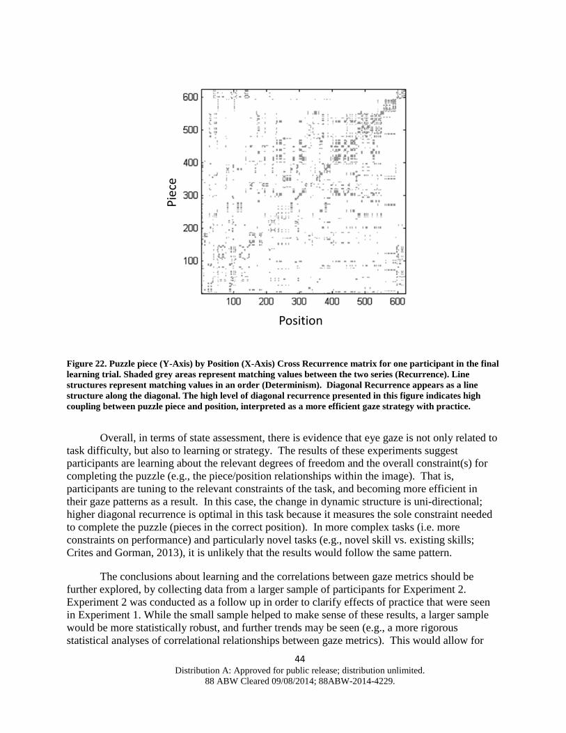
Figure 22. Puzzle piece (Y-Axis) by Position (X-Axis) Cross Recurrence matrix for one participant in the final learning trial. Shaded grey areas represent matching values between the two series (Recurrence). Line structures represent matching values in an order (Determinism). Diagonal Recurrence appears as a line structure along the diagonal. The high level of diagonal recurrence presented in this figure indicates high coupling between puzzle piece and position, interpreted as a more efficient gaze strategy with practice.

Overall, in terms of state assessment, there is evidence that eye gaze is not only related to task difficulty, but also to learning or strategy. The results of these experiments suggest participants are learning about the relevant degrees of freedom and the overall constraint(s) for completing the puzzle (e.g., the piece/position relationships within the image). That is, participants are tuning to the relevant constraints of the task, and becoming more efficient in their gaze patterns as a result. In this case, the change in dynamic structure is uni-directional; higher diagonal recurrence is optimal in this task because it measures the sole constraint needed to complete the puzzle (pieces in the correct position). In more complex tasks (i.e. more constraints on performance) and particularly novel tasks (e.g., novel skill vs. existing skills; Crites and Gorman, 2013), it is unlikely that the results would follow the same pattern.

The conclusions about learning and the correlations between gaze metrics should be further explored, by collecting data from a larger sample of participants for Experiment 2. Experiment 2 was conducted as a follow up in order to clarify effects of practice that were seen in Experiment 1. While the small sample helped to make sense of these results, a larger sample would be more statistically robust, and further trends may be seen (e.g., a more rigorous statistical analyses of correlational relationships between gaze metrics). This would allow for

Piec

e

Position


88 ABW Cleared 09/08/2014; 88ABW-2014-4229.

inferences about shared relationships between variables used in the present work that show correlations with each other. For example, Average Fixation Length and Diagonal Recurrence show a moderate correlation (r = .62) that might approach significance with a larger sample. These relationships could also be further explored via a hierarchical regression analyses to determine the overall contribution of each gaze metric to performance outcomes.

The present studies limited the analyses to the performance outcome of completion time and the different eye gaze metrics. From these analyses, interpretations about strategy were made. The addition of puzzle piece selection and manipulation actions of the participant could provide further insights into operator state. With this data determinations of the specific movement sequences could be assessed. Furthermore, the series of actions could be crossed with eye gaze data, via a cross recurrence analysis, in a similar way as the piece/position cross was implemented here. This could give insight into the coordination of a gaze and action, specifically the degree of coupling between participants’ eye gaze and puzzle manipulation strategies. For example, one potential outcome of these analyses would be the lead/lag relationships between eye gaze and action.

Although eye gaze was singled out in the present study, eye gaze is only one of the potential primary task measures that could be available in an operational setting. Future work could utilize dynamic methods for additional primary measures. For example, communication patterns are one area which has been shown to reveal dynamics of team coordination (Russell et al., 2012). Holden et al.’s (2009; 2011) work on reaction time intervals could also be applied to more general aspect of operational activities (intervals between required actions). Furthermore, variability in control mechanisms (e.g., button presses, flight stick movement) may provide another signal from which to assess operator state using dynamic measures (Strang et al., 2013).

The current project was undertaken with the goal of determining if dynamic patterns of variability in eye gaze reflect underlying properties of an operator. Initially the focus was on workload of the operator, and this project demonstrated the general sensitivity of eye gaze to workload effects. Also demonstrated here was the relationship of dynamic structure to learning or strategy shifts. Support for this idea was confirmed for effects of learning across trials, with some limited support for the idea that dynamic measures were more sensitive than conventional measures in regards to these learning effects. This is not meant to be an indictment of average based measures, rather to stress that not all variability is error; dynamic analyses may provide a richer understanding of underlying states of the operator, but are not necessarily superior to conventional measures. While measures of dynamic structure may be conceptually different from conventional averages, computationally they require little extra effort to compute. Moving forward, both should be applied (where appropriate) to utilize the complimentary explanatory powers in making sense of human performance data in complex tasks.

6.0 REFERENCES

Aks, D.J., Zelinksky, G.J., & Sprott, J.C. (2002). Memory Across Eye-Movements: 1/f Dynamic in Visual Search. Nonlinear Dynamics, Psychology, and Life Sciences, 6(1), 25.

Bassingthwaighte, J.B. (1994). Fractal Physiology: Springer-Verlag.


88 ABW Cleared 09/08/2014; 88ABW-2014-4229.

Carbonell, J.R., Ward, J.L., & Senders, J.W. (1968). A queueing model ofvisual sampling

experimental validation. IEEE transactions on man-machine systems, 9(3), 82-87. Crites, M. J., & Gorman, J. C. (2013). Learning to Tie Well with Others: Bimanual vs.

Intermanual Coordination during Shoe-tying. Paper presented at the Human Factors And Ergonomics Society 57th Annual Meeting, Las Vegas, Nevada.

Davids, K., Button, C., & Bennett, S. (2008). Dynamics of Skill Acquisition: A Constraints-Led

Approach. Champaign, IL: Human Kinetics. Duchowski, A.T. (2002). A Breadth-First Survey of Eye Tracking Applications. Behavior

Research Methods, Instruments, and Computers, 1, 1-16. Eke, A., Herman, P., Kocsis, L., & Kozak, L.R. (2002). Fractal characterization of complexity in

temporal physiological signals. Physiological Measurement, 23, R1-R38. Grier, R., Wickens, C., Kaber, D., Strayer, D., Boehm-Davis, D., Trafton, J.G., & St. John, M.

(2008). The Red-Line of Workload: Theory, Research, and Design. Paper presented at the Human Factors and Ergonomics Society 52nd Annual Meeting, New York, New York.

Guastello, S. J., Boeh, H., Shumaker, C., & Schimmels, M. (2012). Catastrophe models for

cognitive workload and fatigue. Theoretical Issues in Ergonomics Science, 13(5), 586-602.

Harrison, S.J., & Richardson, M.J. (2009). Horsing around: spontaneous four-legged

coordination. Journal of Motor Behavior, 41(6), 519-524. Hayhoe, M., Bensinger, D.G., & Ballard, D.H. (1998). Task constraints in visual working

memory. Vision Research, 38(1), 124-137. Heinen, S.J., Jin, Z., & Watamaniuk, S.N.J. (2011). Flexibility of foveal attention during ocular

pursuit. Journal of Vision, 11, 1-12. Holden, J.G., Van Orden, G.C., & Turvey, M. T. (2009). Dispersion of Response Times Reveals

Cognitive Dynamics. Psychological Review, 116(2), 318-342.


88 ABW Cleared 09/08/2014; 88ABW-2014-4229.

Holden, J. G., Choi, I., Amazeen, P.G., & Van Orden, G.C. (2011). Fractal 1/ƒ Dynamics Suggest Entanglement of Measurement and Human Performance. Journal of experimental psychology: Human Perception and Performance, 37(3), 935-948.

Jensen, H.J. (1998). Self-organized Criticality. Cambridge: Cambridge Univ. Press. Jorna, P.G.A.M. (1992). Spectral analysis of heart rate and psychological state: A review of its

validity as a workload index. Biological psychology, 34, 237-257. Kelso, J.A.S. (1995). Dynamic Patterns. Cambridge, MA: MIT Press. Kloos, H., & Van Orden, G.C. (2010). Voluntary behavior in cognitive and motor tasks. Mind &

Matter, 8(1), 19-43. Kowler, E. (2011). Eye movements: The past 25 years. Vision Research, 51, 1457-1483. Kugler, P.N., Kelso, J.A.S., & Turvey, M. T. (1982). On the control and co-ordination of

naturally developing systems. In J. A. S. Kelso & J. E. Clark (Eds.), The Development of Movement Control and Co-Ordination: Wiley & Sons.

Land, M.F., & Hayhoe, M. (2001). In what ways do eye movments contribute to everyday

activities? Vision Research, 41(25-26), 3559-3565. Newman, M.E.J. (2005). Power laws, Pareto distributions and Zipf's law. Contemporary Physics,

46(5), 323-351. O'Donnell, R., & Eggemeier, F.T. (1986). Workload assessment methodology. In K. R. Boff, L.

Kaufman & J. P. Thomas (Eds.), Handbook of perception and human performance: Vol.2. Cognitive processes and performance (Vol. Wiley). New York.

Ogden, G. D., Levine, J. M., & Eisner, E. J. (1979). Measurement of workload by secondary

tasks. Human Factors: The Journal of the Human Factors and Ergonomics Society, 21, 529-548.

Parasuraman, R., & Galster, S. (2013). Sensing, assessing, and augmenting threat detection:

behavioral, neuroimaging, and brain stimulation evidence for the critical role of attention. Frontiers in Human Neuroscience, 7, 1-10.

Posner, M., Snyder, C., & Davidson, B. (1980). Attention and the detection of signals. Journal of

Experimental Psychology: General, 109(2), 160-174. 47

Distribution A: Approved for public release; distribution unlimited. 88 ABW Cleared 09/08/2014; 88ABW-2014-4229.

Rayner, K. (1998). Eye movments in reading and information processing. Psychological

Bulletin, 124(3), 372-422. Richardson, D.C., & Dale, R. (2005). Looking To Understand: The Coupling Between Speakers’

and Listeners’ Eye Movements and its Relationship to Discourse Comprehension. Cognitive Science, 29, 35-54.

Russell, S.M., Funke, G.J., Knott, B.A., & Strang, A.J. (2012). Recurrence quantification

analysis used to assess team communication in simulated air battle management. Paper presented at the Human Factors and Ergonomics Society 56th Annual Meeting, Boston, MA.

Salvucci, D. D., & Goldberg, J. H. (2000). Identifying fixations and saccades in eye-tracking

protocols. Paper presented at the Eye Tracking Research and Applications Symposium, New York.

Silver, N.C., & Dunlap, W.P. (1987). Averaging correlation coefficients: should Fisher's z

transformation be used? Journal of Applied Psychology, 72(1), 146-148. Stephen, D.G., & Anastas, J. (2011). Fractal fluctuations in gaze speed visual search. Attention,

Perception, & Psychophysics, 73, 666-677. Stephen, D.G., & Mirman, D. (2010). Interactions dominate the dynamics of visual cognition.

Cognition, 115, 154-165. Strang, A.J., Epling, S., Funke, G.J., & Russell, S.M. (2013). Temporal Complexity in team

coordination associated with increased performance in a fast-paced puzzle task. Paper presented at the Human Factors and Ergonomics society 57th Annual Meeting, Las Vegas, NV.

Stratton, S.M., Liu, Y.T., Hong, S.L., mayer-Kress, G., & Newell, K.M. (2007). Snoddy (1926)

revisited: time scales of motor learning. Journal of Motor Behavior, 39, 503-515. Takens, F. (1981). Detecting strange attractors in turbulence. Lecture Notes in Mathematics, 898,

366-381. Tatler, B.W., Wade, N.J., Kwan, H., Findlay, J.M., & Velichkovsky, B.M. (2010). Yarbus, eye

movements, and vision. i-Perception, 1(1), 7-27.


88 ABW Cleared 09/08/2014; 88ABW-2014-4229.

Tsang, P. S., & Vidulich, M. A. (2006). Mental workload and situation awareness. Handbook of Human Factors and Ergonomics, Third Edition, 243-268.

Van Orden, G.C., Holden, J. G., & Turvey, M. T. (2005). Human Cognition and 1/f Scaling.

Journal of Experimental Psychology: General, 134(1), 117-123. Warm, J. S., Parasuraman, R., & Matthews, G. (2008). Vigilance Requires Hard Mental Work

and Is Stressful. Human Factors: The Journal of the Human Factors and Ergonomics Society, 50(3), 433-441.

Warren, W.H. (2006). The dynamics of perception and action. Psychological Review, 113(2),

358-389. Webber, C.L., & Zbilut, J.P. (2005). Recurrence quantification analysis of nonlinear dynamical

systems. In M. A. Riley & G. C. Van Orden (Eds.), Tutorials in contemporary nonlinear mehtods for the behaviorl sciences (pp. 26-94).

Wickens, C. D. (2002). Multiple resources and performance prediction.Theoretical issues in

ergonomics science, 3(2), 159-177. Wilson, G.F. (2002). An Analysis of Mental Workload in Pilots During Flight Using Multiple

Psychophysiological Measures. The International Version of Aviation Psychology, 12(1), 3-18.

Yarbus. (1967). Eye Movements and Vision: Plenum.


88 ABW Cleared 09/08/2014; 88ABW-2014-4229.

Documents

ALTERNATIVE INDICES OF PERFORMANCE: AN …