Embed Size (px)
Citation preview
1/18/2009 (C) 2009 Best-Fit Computing, Inc. 1
ALTA
Relative Positional
Accuracy
Instructor
Scott Wallace
1/18/2009 (C) 2009 Best-Fit Computing, Inc. 2
Agenda
1. Relative Positional Accuracy
2. The Mathematical Test
3. Statistical Review
4. Computing The Error Ellipse
5. Sample Network Projects
6. Network Design
7. Tips For Success
1/18/2009 (C) 2009 Best-Fit Computing, Inc. 3
1. Relative Positional Accuracy
“Relative Positional Accuracy (RPA) is the value expressed in feet or meters that represents the uncertainty due to random errors in measurements in the location of any point on a survey to any other point on the same survey, at the 95 percent confidence level.” Rule 12, 865 IAC, 1-12-2.
The ALTA (American Land Title Association) test is based on the relative error ellipse and the horizontal distance between each station pair. The relative error ellipse represents the relative precision of each station pair. This test was jointly developed by ALTA and the American Congress on Surveying and Mapping (ACSM).
RPA may be tested by:
1. Comparing the relative location of points in a survey as measured by an independent survey of higher accuracy.
2. Testing the results from a minimally-constrained, correctly weighted, least squares adjustment of the survey.
1/18/2009 (C) 2009 Best-Fit Computing, Inc. 4
1. Relative Positional Accuracy
WHY Least Squares
1. Distributes the error following laws of random probability.
2. Only way to handle complex networks.
3. Minimizes the sum of squared residuals.
4. The best any other method can do is to equal the results of a least squares adjustment.
REQUIREMENTS for valid results
1. Instruments properly tuned.
2. Proper field procedures used.
3. Blunders and systematic errors removed or minimized.
4. Remaining inaccuracy is due to random errors.
PROCEDURE
1. Minimally-constrained adjustment tied to one station + a direction (azimuth, bearing or a vector).
2. Proper weighting employed by assigning expected errors (standard deviations) to observations.
1/18/2009 (C) 2009 Best-Fit Computing, Inc. 5
2. The Mathematical Test
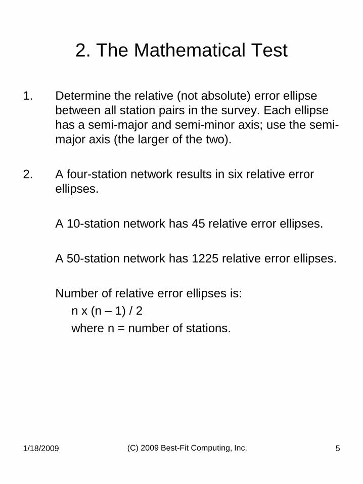
1. Determine the relative (not absolute) error ellipse
between all station pairs in the survey. Each ellipse
has a semi-major and semi-minor axis; use the semi-
major axis (the larger of the two).
2. A four-station network results in six relative error
ellipses.
A 10-station network has 45 relative error ellipses.
A 50-station network has 1225 relative error ellipses.
Number of relative error ellipses is:
n x (n – 1) / 2
where n = number of stations.
1/18/2009 (C) 2009 Best-Fit Computing, Inc. 6
2. The Mathematical Test
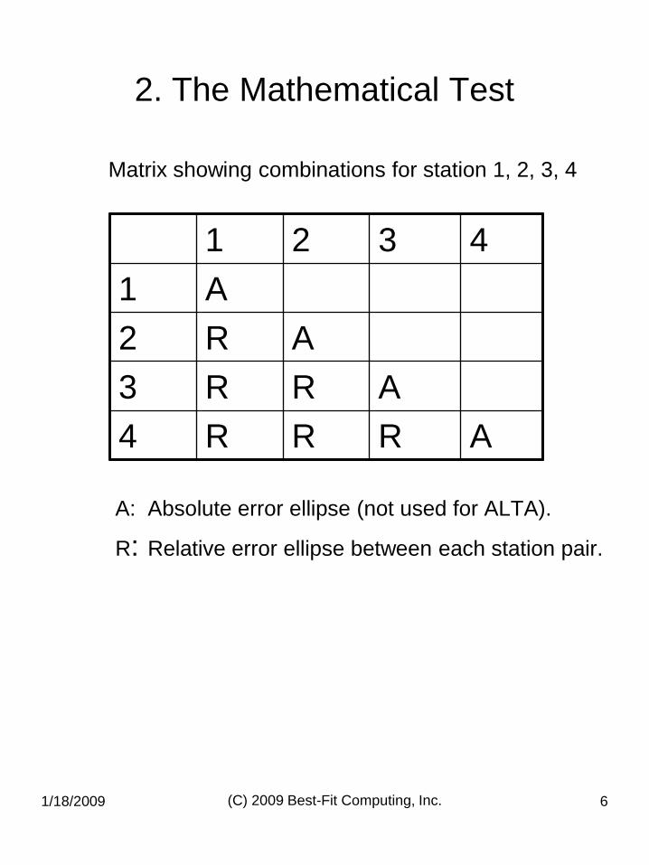
A: Absolute error ellipse (not used for ALTA).
R: Relative error ellipse between each station pair.
1 2 3 4
1 A
2 R A
3 R R A
4 R R R A
Matrix showing combinations for station 1, 2, 3, 4
1/18/2009 (C) 2009 Best-Fit Computing, Inc. 7
2. The Mathematical Test
3. Scale the semi-major ellipse to the 95% confidence level using the K value of 2.448.
4. Compute the total allowable uncertainty for each station pair using the fixed tolerance and the variable PPM (Parts Per Million).
Total Tolerance Allowed
0.07 feet + 50 PPM
The PPM contribution increases with increasing horizontal distance between any two station pairs.
5. The ratio of the scaled relative error ellipse to the Total Tolerance Allowed must be <= 1.0.
1/18/2009 (C) 2009 Best-Fit Computing, Inc. 8
2. The Mathematical Test
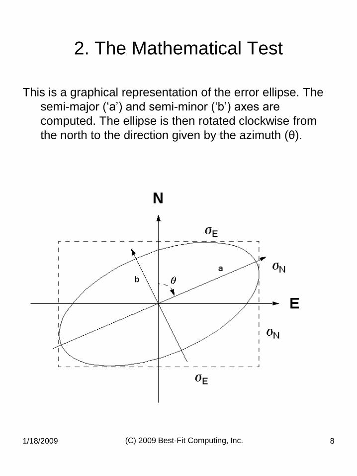
This is a graphical representation of the error ellipse. The
semi-major („a‟) and semi-minor („b‟) axes are
computed. The ellipse is then rotated clockwise from
the north to the direction given by the azimuth (θ).
1/18/2009 (C) 2009 Best-Fit Computing, Inc. 9
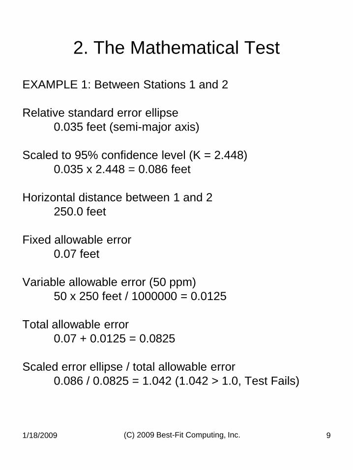
2. The Mathematical Test
EXAMPLE 1: Between Stations 1 and 2
Relative standard error ellipse
0.035 feet (semi-major axis)
Scaled to 95% confidence level (K = 2.448)
0.035 x 2.448 = 0.086 feet
Horizontal distance between 1 and 2
250.0 feet
Fixed allowable error
0.07 feet
Variable allowable error (50 ppm)
50 x 250 feet / 1000000 = 0.0125
Total allowable error
0.07 + 0.0125 = 0.0825
Scaled error ellipse / total allowable error
0.086 / 0.0825 = 1.042 (1.042 > 1.0, Test Fails)
1/18/2009 (C) 2009 Best-Fit Computing, Inc. 10
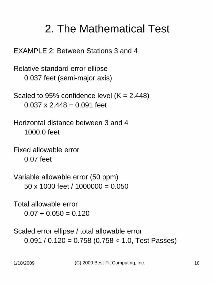
2. The Mathematical Test
EXAMPLE 2: Between Stations 3 and 4
Relative standard error ellipse
0.037 feet (semi-major axis)
Scaled to 95% confidence level (K = 2.448)
0.037 x 2.448 = 0.091 feet
Horizontal distance between 3 and 4
1000.0 feet
Fixed allowable error
0.07 feet
Variable allowable error (50 ppm)
50 x 1000 feet / 1000000 = 0.050
Total allowable error
0.07 + 0.050 = 0.120
Scaled error ellipse / total allowable error
0.091 / 0.120 = 0.758 (0.758 < 1.0, Test Passes)
1/18/2009 (C) 2009 Best-Fit Computing, Inc. 11
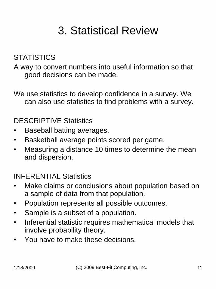
3. Statistical Review
STATISTICS
A way to convert numbers into useful information so that good decisions can be made.
We use statistics to develop confidence in a survey. We can also use statistics to find problems with a survey.
DESCRIPTIVE Statistics
• Baseball batting averages.
• Basketball average points scored per game.
• Measuring a distance 10 times to determine the mean and dispersion.
INFERENTIAL Statistics
• Make claims or conclusions about population based on a sample of data from that population.
• Population represents all possible outcomes.
• Sample is a subset of a population.
• Inferential statistic requires mathematical models that involve probability theory.
• You have to make these decisions.
1/18/2009 (C) 2009 Best-Fit Computing, Inc. 12
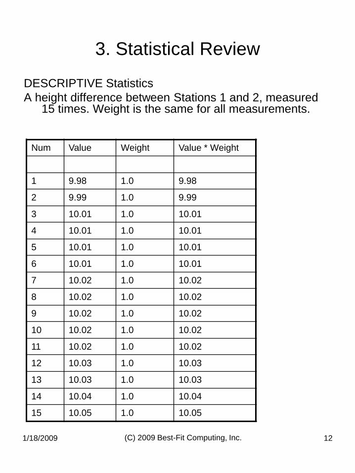
3. Statistical Review
DESCRIPTIVE Statistics
A height difference between Stations 1 and 2, measured 15 times. Weight is the same for all measurements.
Num Value Weight Value * Weight
1 9.98 1.0 9.98
2 9.99 1.0 9.99
3 10.01 1.0 10.01
4 10.01 1.0 10.01
5 10.01 1.0 10.01
6 10.01 1.0 10.01
7 10.02 1.0 10.02
8 10.02 1.0 10.02
9 10.02 1.0 10.02
10 10.02 1.0 10.02
11 10.02 1.0 10.02
12 10.03 1.0 10.03
13 10.03 1.0 10.03
14 10.04 1.0 10.04
15 10.05 1.0 10.05
1/18/2009 (C) 2009 Best-Fit Computing, Inc. 13
3. Statistical Review
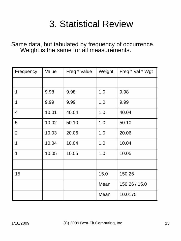
Same data, but tabulated by frequency of occurrence. Weight is the same for all measurements.
Frequency Value Freq * Value Weight Freq * Val * Wgt
1 9.98 9.98 1.0 9.98
1 9.99 9.99 1.0 9.99
4 10.01 40.04 1.0 40.04
5 10.02 50.10 1.0 50.10
2 10.03 20.06 1.0 20.06
1 10.04 10.04 1.0 10.04
1 10.05 10.05 1.0 10.05
15 15.0 150.26
Mean 150.26 / 15.0
Mean 10.0175
1/18/2009 (C) 2009 Best-Fit Computing, Inc. 14
3. Statistical Review
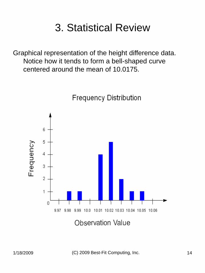
Graphical representation of the height difference data.
Notice how it tends to form a bell-shaped curve
centered around the mean of 10.0175.
1/18/2009 (C) 2009 Best-Fit Computing, Inc. 15
3. Statistical Review
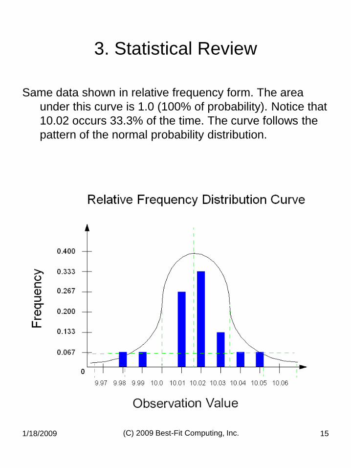
Same data shown in relative frequency form. The area
under this curve is 1.0 (100% of probability). Notice that
10.02 occurs 33.3% of the time. The curve follows the
pattern of the normal probability distribution.
1/18/2009 (C) 2009 Best-Fit Computing, Inc. 16
3. Statistical Review
CALCULATING Descriptive Statistics
Measures of Central Tendency (center point of data set):
Mean - Arithmetic mean
Median - Mid Point Value (half below, half above)
Mode - Most common value
Xi - i‟th observation value
Wi - i‟th observation weight (all 1.0 in this example)
Mean - (summation all Xi * Wi) / (summation all Wi)
- 150.26 / 15.0
- 10.017
Median - 10.02
Mode - 10.02
The Mean is the least squares solution. In this example,
10.017 results in the minimization of the sum of
squared weighted residuals, where the weight for each
observation is 1.0.
1/18/2009 (C) 2009 Best-Fit Computing, Inc. 17
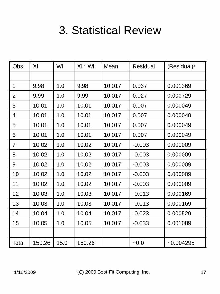
3. Statistical Review
Obs Xi Wi Xi * Wi Mean Residual (Residual)2
1 9.98 1.0 9.98 10.017 0.037 0.001369
2 9.99 1.0 9.99 10.017 0.027 0.000729
3 10.01 1.0 10.01 10.017 0.007 0.000049
4 10.01 1.0 10.01 10.017 0.007 0.000049
5 10.01 1.0 10.01 10.017 0.007 0.000049
6 10.01 1.0 10.01 10.017 0.007 0.000049
7 10.02 1.0 10.02 10.017 -0.003 0.000009
8 10.02 1.0 10.02 10.017 -0.003 0.000009
9 10.02 1.0 10.02 10.017 -0.003 0.000009
10 10.02 1.0 10.02 10.017 -0.003 0.000009
11 10.02 1.0 10.02 10.017 -0.003 0.000009
12 10.03 1.0 10.03 10.017 -0.013 0.000169
13 10.03 1.0 10.03 10.017 -0.013 0.000169
14 10.04 1.0 10.04 10.017 -0.023 0.000529
15 10.05 1.0 10.05 10.017 -0.033 0.001089
Total 150.26 15.0 150.26 ~0.0 ~0.004295
1/18/2009 (C) 2009 Best-Fit Computing, Inc. 18
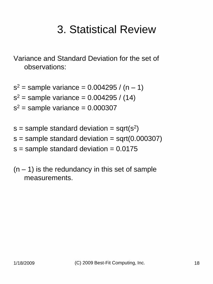
3. Statistical Review
Variance and Standard Deviation for the set of
observations:
s2 = sample variance = 0.004295 / (n – 1)
s2 = sample variance = 0.004295 / (14)
s2 = sample variance = 0.000307
s = sample standard deviation = sqrt(s2)
s = sample standard deviation = sqrt(0.000307)
s = sample standard deviation = 0.0175
(n – 1) is the redundancy in this set of sample
measurements.
1/18/2009 (C) 2009 Best-Fit Computing, Inc. 19
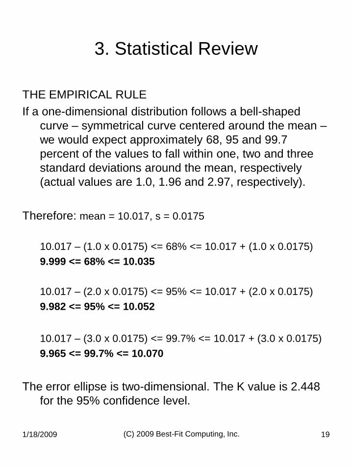
3. Statistical Review
THE EMPIRICAL RULE
If a one-dimensional distribution follows a bell-shaped
curve – symmetrical curve centered around the mean –
we would expect approximately 68, 95 and 99.7
percent of the values to fall within one, two and three
standard deviations around the mean, respectively
(actual values are 1.0, 1.96 and 2.97, respectively).
Therefore: mean = 10.017, s = 0.0175
10.017 – (1.0 x 0.0175) <= 68% <= 10.017 + (1.0 x 0.0175)
9.999 <= 68% <= 10.035
10.017 – (2.0 x 0.0175) <= 95% <= 10.017 + (2.0 x 0.0175)
9.982 <= 95% <= 10.052
10.017 – (3.0 x 0.0175) <= 99.7% <= 10.017 + (3.0 x 0.0175)
9.965 <= 99.7% <= 10.070
The error ellipse is two-dimensional. The K value is 2.448
for the 95% confidence level.
1/18/2009 (C) 2009 Best-Fit Computing, Inc. 20
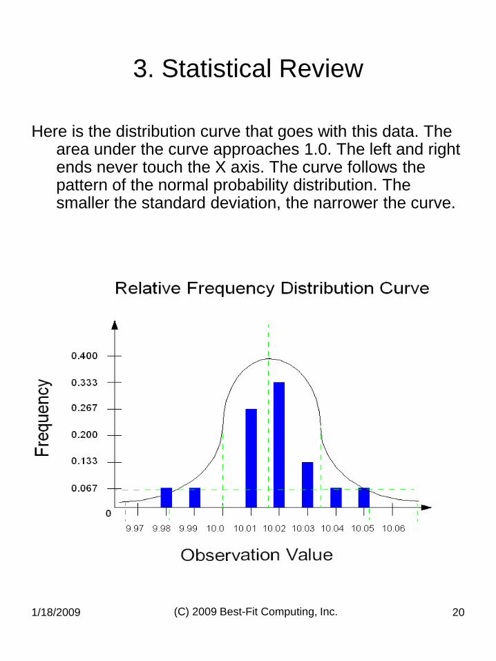
3. Statistical Review
Here is the distribution curve that goes with this data. The area under the curve approaches 1.0. The left and right ends never touch the X axis. The curve follows the pattern of the normal probability distribution. The smaller the standard deviation, the narrower the curve.
1/18/2009 (C) 2009 Best-Fit Computing, Inc. 21
3. Statistical Review
The mean of all sample observations is the best-fit, least squares solution.
STANDARD deviation of the mean
s mean = s / sqrt(num observations)
s mean = 0.0175 / sqrt(15.0)
s mean = 0.004518
VARIANCE of the mean
s2 mean = s mean * s mean
s2 mean = ~0.000020417
This is what you would expect if you measured the same height difference 15 times, each day, for 10 or 20 days. The mean of each day‟s work would follow a normal distribution. The standard deviation and variance of these means would be much smaller than that for an individual set of observations.
If we load this data into an adjustment, we will see this result for the adjusted height standard deviation (LevelNet.txt).
1/18/2009 (C) 2009 Best-Fit Computing, Inc. 22
3. Statistical Review
ABSOLUTE Error Ellipse
The absolute standard error ellipse is a representation of a probability. We really do not know in absolute terms where the point we measured really is; we only have a probability of where the point is.
A standard error ellipse (un-scaled) represents a 60.6% chance that the actual point is outside the computed position and the area bounded by the standard error ellipse. To ensure a smaller probability that the point is outside this region, the size of the standard error ellipse must be increased.
By expanding the standard error ellipse by the K value of 2.448, we create a 5% probability that the point may fall outside the computed position and the area bounded by the standard error ellipse. Put another way, the point has a 95% probability of falling within this region, the standard error ellipse is scaled by 2.448.
1/18/2009 (C) 2009 Best-Fit Computing, Inc. 23
3. Statistical Review
RELATIVE Error Ellipse
The standard relative error ellipse is a representation of the relative precision of each station pair coordinate difference. This ellipse is created by differencing the coordinate errors for each station pair. Errors common to both stations are eliminated.
The standard relative error ellipse can be smaller than the absolute (station) error ellipse on each end. The coordinates for each station could be completely wrong (e.g., based on incorrectly used fixed coordinates), but the relative errors between stations give the best estimate of the precision of the survey – regardless of the coordinates.
Think in terms of GPS measurements. The station coordinates determined using GPS may be off by meters, but the vector (the difference between these coordinates) can be accurate to the centimeter level or better. The error in this vector is the best indicator as to the quality of the measurement.
To scale the standard relative error ellipse to the 95% confidence level, use a K value of 2.448.
1/18/2009 (C) 2009 Best-Fit Computing, Inc. 24
3. Statistical Review
TYPE I Error
In the previous discussion, we implied that we have a 5% probability that the actual point falls outside the computed coordinate value and the bounding error ellipse. There is a 95% chance that the value falls inside this region.
Ho is the Null Hypothesis (the hypothesis that the true position of the coordinate falls within the computed coordinate value and the bounding error ellipse).
A Type I error is committed when Ho is rejected based on a statistical test of sample data when, in fact, Ho is true. The probability of committing this type of error is 5% (or alpha), when the confidence level is set to 95%.
Suppose the computer-generated statistics tell us to reject Ho. We would reject the result, even though it is correct. Fortunately, this only has a 5% chance of occurring. If we reject Ho when it was really true, we may need additional field work to confirm that the original data, is in fact, acceptable data.
1/18/2009 (C) 2009 Best-Fit Computing, Inc. 25
3. Statistical Review
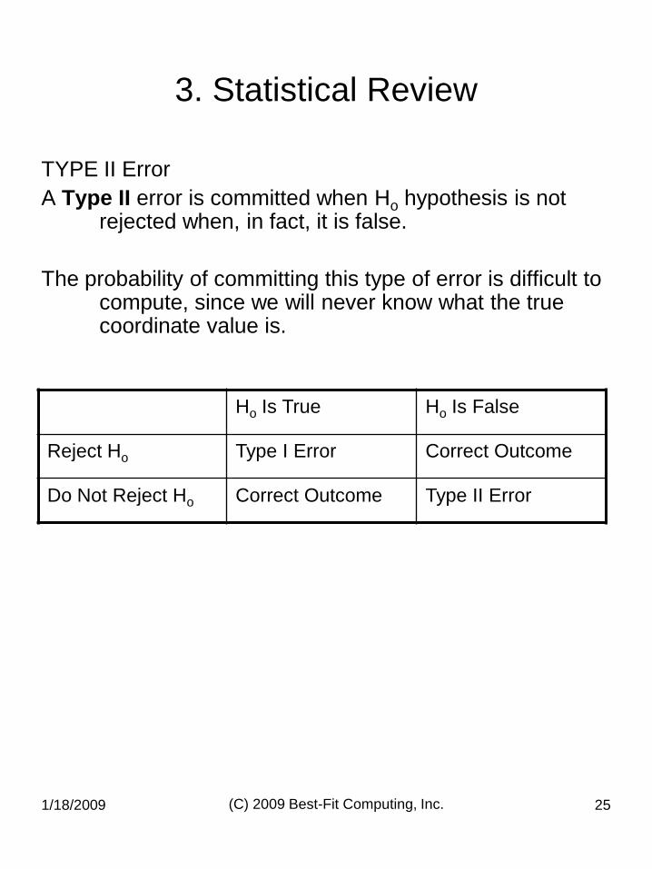
TYPE II Error
A Type II error is committed when Ho hypothesis is not rejected when, in fact, it is false.
The probability of committing this type of error is difficult to compute, since we will never know what the true coordinate value is.
Ho Is True Ho Is False
Reject Ho Type I Error Correct Outcome
Do Not Reject Ho Correct Outcome Type II Error
1/18/2009 (C) 2009 Best-Fit Computing, Inc. 26
4. Computing The Error Ellipse
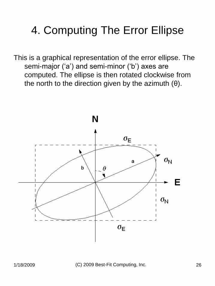
This is a graphical representation of the error ellipse. The
semi-major („a‟) and semi-minor („b‟) axes are
computed. The ellipse is then rotated clockwise from
the north to the direction given by the azimuth (θ).
1/18/2009 (C) 2009 Best-Fit Computing, Inc. 27
4. Computing The Error Ellipse
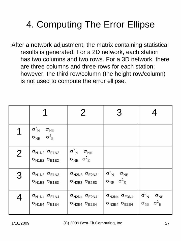
After a network adjustment, the matrix containing statistical
results is generated. For a 2D network, each station
has two columns and two rows. For a 3D network, there
are three columns and three rows for each station;
however, the third row/column (the height row/column)
is not used to compute the error ellipse.
1 2 3 4
1 s2N sNE
sNE s2
E
2 sN1N2 sE1N2
sN1E2 sE1E2
s2N sNE
sNE s2
E
3 sN1N3 sE1N3
sN1E3 sE1E3
sN2N3 sE2N3
sN2E3 sE2E3
s2N sNE
sNE s2
E
4 sN1N4 sE1N4
sN1E4 sE1E4
sN2N4 sE2N4
sN2E4 sE2E4
sN3N4 sE3N4
sN3E4 sE3E4
s2N sNE
sNE s2
E
1/18/2009 (C) 2009 Best-Fit Computing, Inc. 28
4. Computing The Error Ellipse
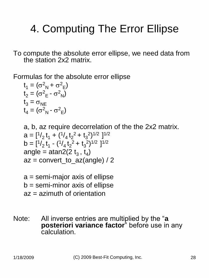
To compute the absolute error ellipse, we need data from the station 2x2 matrix.
Formulas for the absolute error ellipse
t1 = (s2N + s2
E)
t2 = (s2E - s2
N)
t3 = sNE
t4 = (s2N - s2
E)
a, b, az require decorrelation of the the 2x2 matrix.
a = [1/2 t1 + (1/4 t22 + t3
2)1/2 ]1/2
b = [1/2 t1 - (1/4 t22 + t3
2)1/2 ]1/2
angle = atan2(2 t3 , t4)
az = convert_to_az(angle) / 2
a = semi-major axis of ellipse
b = semi-minor axis of ellipse
az = azimuth of orientation
Note: All inverse entries are multiplied by the “a posteriori variance factor” before use in any calculation.
1/18/2009 (C) 2009 Best-Fit Computing, Inc. 29
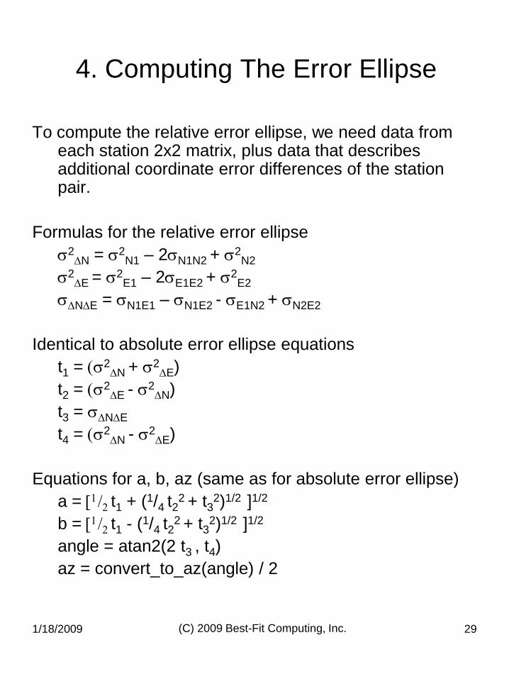
4. Computing The Error Ellipse
To compute the relative error ellipse, we need data from each station 2x2 matrix, plus data that describes additional coordinate error differences of the station pair.
Formulas for the relative error ellipse
s2DN = s2
N1 – 2sN1N2 + s2N2
s2DE = s2
E1 – 2sE1E2 + s2E2
sDNDE = sN1E1 – sN1E2 - sE1N2 + sN2E2
Identical to absolute error ellipse equations
t1 = (s2DN + s2
DE)
t2 = (s2DE - s2
DN)
t3 = sDNDE
t4 = (s2DN - s2
DE)
Equations for a, b, az (same as for absolute error ellipse)
a = [1/2 t1 + (1/4 t22 + t3
2)1/2 ]1/2
b = [1/2 t1 - (1/4 t22 + t3
2)1/2 ]1/2
angle = atan2(2 t3 , t4)
az = convert_to_az(angle) / 2
1/18/2009 (C) 2009 Best-Fit Computing, Inc. 30
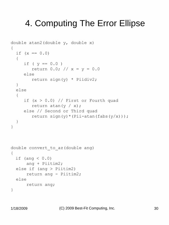
4. Computing The Error Ellipse
double atan2(double y, double x)
{
if (x == 0.0)
{
if ( y == 0.0 )
return 0.0; // x = y = 0.0
else
return sign(y) * Piidiv2;
}
else
{
if (x > 0.0) // First or Fourth quad
return atan(y / x);
else // Second or Third quad
return sign(y)*(Pii-atan(fabs(y/x)));
}
}
double convert_to_az(double ang)
{
if (ang < 0.0)
ang + Piitim2;
else if (ang > Piitim2)
return ang - Piitim2;
else
return ang;
}
1/18/2009 (C) 2009 Best-Fit Computing, Inc. 31
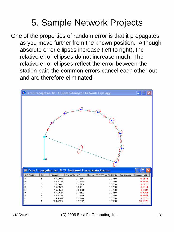
5. Sample Network Projects
One of the properties of random error is that it propagates
as you move further from the known position. Although
absolute error ellipses increase (left to right), the
relative error ellipses do not increase much. The
relative error ellipses reflect the error between the
station pair; the common errors cancel each other out
and are therefore eliminated.
1/18/2009 (C) 2009 Best-Fit Computing, Inc. 32
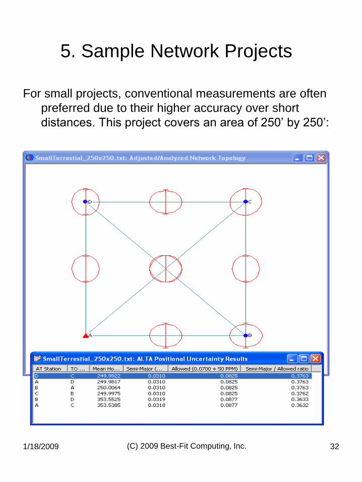
5. Sample Network Projects
For small projects, conventional measurements are often
preferred due to their higher accuracy over short
distances. This project covers an area of 250‟ by 250‟:
1/18/2009 (C) 2009 Best-Fit Computing, Inc. 33
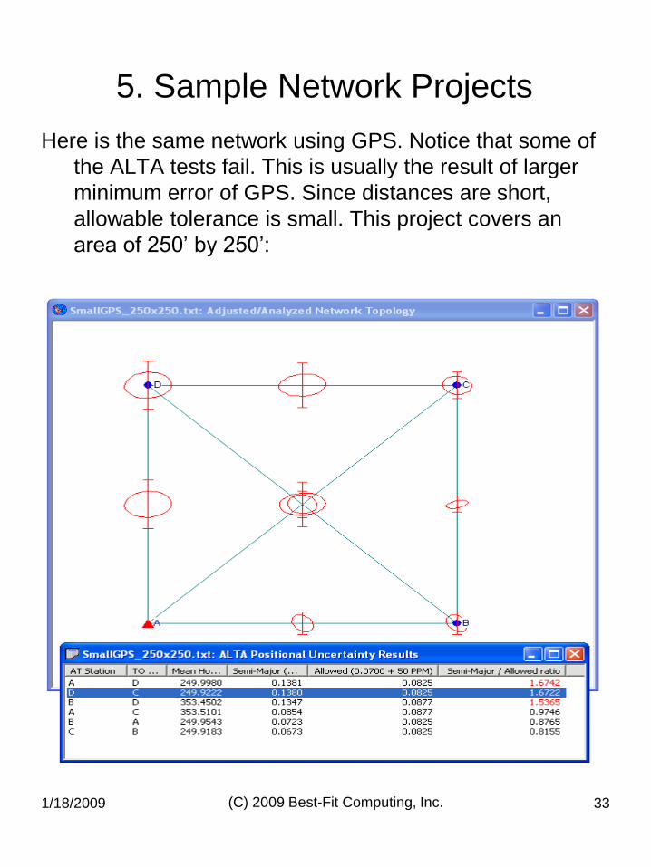
5. Sample Network Projects
Here is the same network using GPS. Notice that some of
the ALTA tests fail. This is usually the result of larger
minimum error of GPS. Since distances are short,
allowable tolerance is small. This project covers an
area of 250‟ by 250‟:
1/18/2009 (C) 2009 Best-Fit Computing, Inc. 34
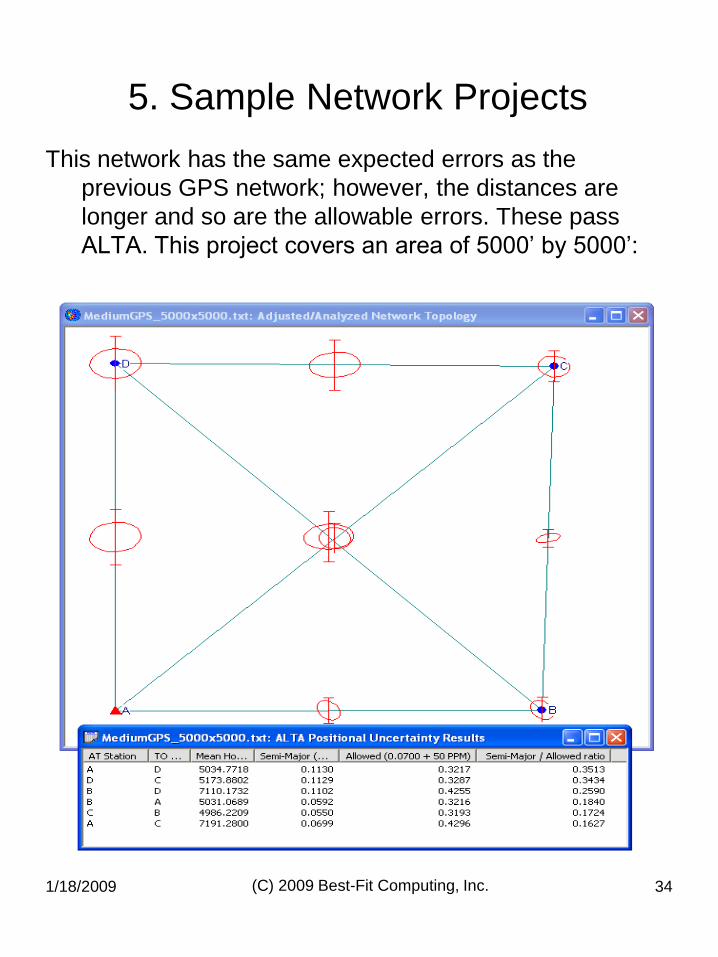
5. Sample Network Projects
This network has the same expected errors as the
previous GPS network; however, the distances are
longer and so are the allowable errors. These pass
ALTA. This project covers an area of 5000‟ by 5000‟:
1/18/2009 (C) 2009 Best-Fit Computing, Inc. 35
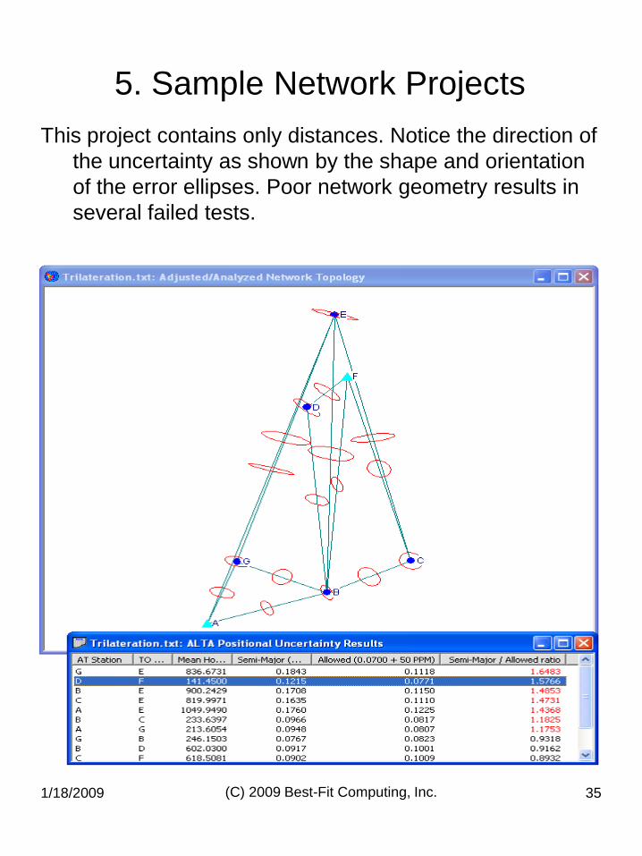
5. Sample Network Projects
This project contains only distances. Notice the direction of
the uncertainty as shown by the shape and orientation
of the error ellipses. Poor network geometry results in
several failed tests.
1/18/2009 (C) 2009 Best-Fit Computing, Inc. 36
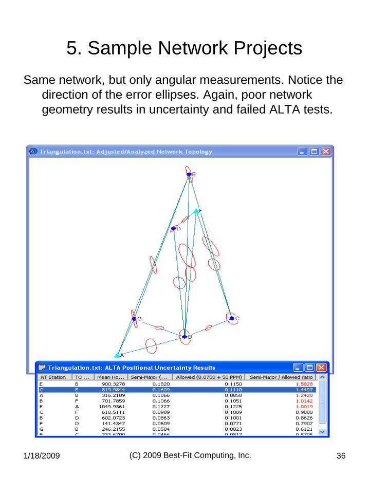
5. Sample Network Projects
Same network, but only angular measurements. Notice the
direction of the error ellipses. Again, poor network
geometry results in uncertainty and failed ALTA tests.
1/18/2009 (C) 2009 Best-Fit Computing, Inc. 37
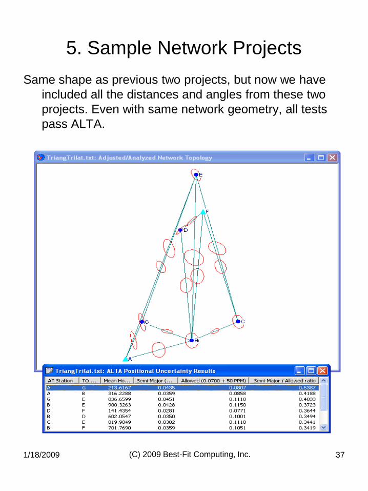
5. Sample Network Projects
Same shape as previous two projects, but now we have
included all the distances and angles from these two
projects. Even with same network geometry, all tests
pass ALTA.
1/18/2009 (C) 2009 Best-Fit Computing, Inc. 38
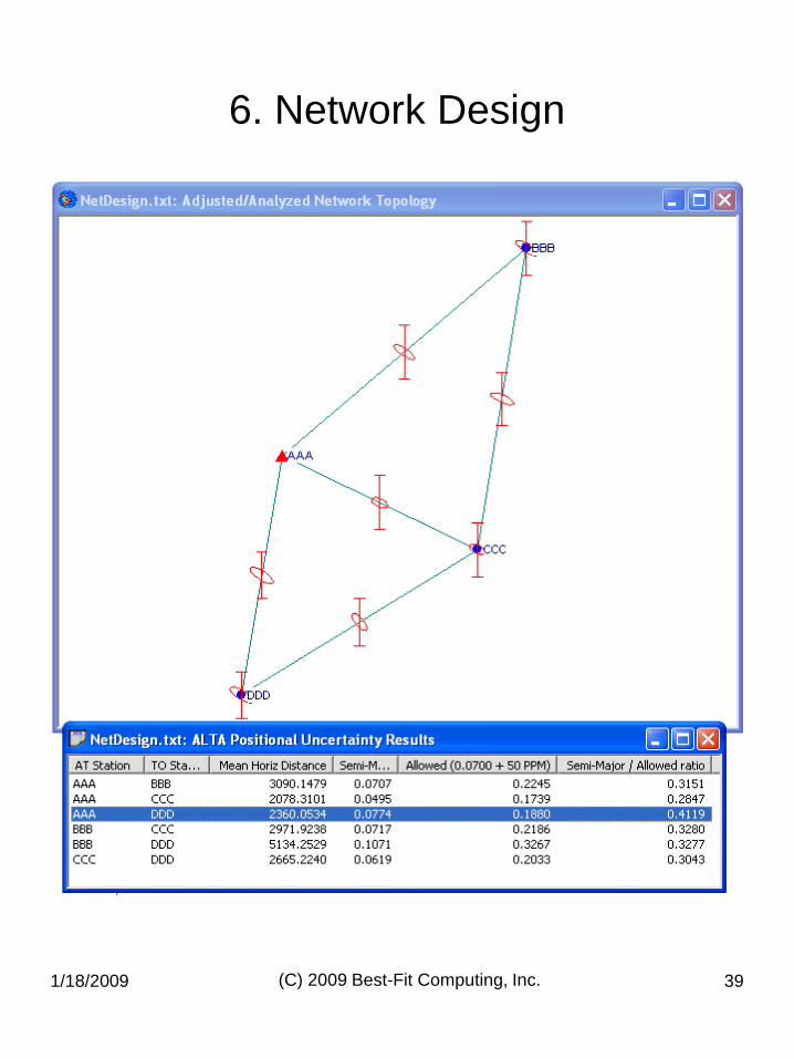
6. Network Design
Network design allows you to determine, in advance, if
your survey will meet ALTA requirements. For
network design, you need the following:
1. Approximate coordinates of surveyed locations.
2. The type of observations used between each station
pair.
3. The expected error in your measurements (as
expressed by the standard deviation of each
observation).
If your design is adequate and you meet or exceed the
expected error (in the field), the survey should pass
ALTA testing.
SAMPLE Project
Stations: AAA, BBB, CCC, DDD.
Hor Ang, Zen Ang, Slope Dist between each station.
SD‟s are 4.0, 7.0 sec and 0.01‟ respectively
Az from AAA to CCC for orientation (SD=1.0 sec).
Slope Dist from CCC to AAA (SD=0.01‟).
1/18/2009 (C) 2009 Best-Fit Computing, Inc. 39
6. Network Design
1/18/2009 (C) 2009 Best-Fit Computing, Inc. 40
7. Tips For Success
1. Equipment and crew must be well-functioning.
2. Utilize good network geometry: equilateral triangles for terrestrial observations and sky geometry for satellites.
3. Check field data daily, if possible. This makes it much easier to find blunders.
4. Use realistic standard deviations.
5. Eliminate systematic errors and blunders; use statistical tests to help identify outliers.
6. For large scale projects, use ellipsoidal height when adjusting in 3D. Using elevation can introduce a onePPM error for every six meters in height difference between the elevation value and the ellipsoidal height value.
7. Utilize Network Design as often as possible.