1

ALMA MATER STUDIORUM - UNIVERSITÀ DI BOLOGNA

SCUOLA DI INGEGNERIA E ARCHITETTURA

CORSO DI LAUREA MAGISTRALE IN INGEGNERIA PER L'AMBIENTE E IL TERRITORIO

DICAM

Dipartimento di Ingegneria Civile, Chimica, Ambientale e dei Materiali

RESEARCH B

In:

Laboratory On Alternative And Renewable Raw Materials

Biogas and bio-hydrogen: production and uses. A review

Candidato: Relatore: Lorenzo APPRESSI Prof. Ing. Lorenzo BERTIN

Anno Accademico 2014-15

Sessione I

2

TABLE OF CONTENTS

ABSTRACT ...................................................................................................................................................... 4

1. INTRODUCTION ......................................................................................................................................... 6

1.1. Bio-refineries ..................................................................................................................................... 7

2. ANAEROBIC DIGESTION ........................................................................................................................... 10

2.1. Recalls on the metabolism of living organisms ............................................................................... 11

2.2. Methanogens ................................................................................................................................... 13

2.2.1. Substrate specificity ................................................................................................................. 13

2.2.2. pH............................................................................................................................................. 14

2.2.3. Temperature ............................................................................................................................ 14

2.2.4. Toxic elements ......................................................................................................................... 15

2.2.5. Habitats .................................................................................................................................... 16

2.3. Stages of the anaerobic digestion ................................................................................................... 16

2.3.1. Hydrolysis ................................................................................................................................ 18

2.3.2. Acidogenesis ............................................................................................................................ 18

2.3.3. Acetogenesis ............................................................................................................................ 19

2.3.4. Methanogenesis ...................................................................................................................... 19

3. INDUSTRIAL PROCESS .............................................................................................................................. 21

3.1. Substrate characterisation .............................................................................................................. 21

3.1.1. Co-digestion ............................................................................................................................. 22

3.1.2. Energy crops ............................................................................................................................ 23

3.1.3. Animal by-products ................................................................................................................. 24

3.2. Reactor parameters ......................................................................................................................... 24

3.3. Continuity in single-stage processes ............................................................................................... 27

3.3.1. Continuous processes .............................................................................................................. 27

3.3.2. Batch processes ....................................................................................................................... 30

3.3.3. Fed-batch processes ................................................................................................................ 31

3.4. Moisture .......................................................................................................................................... 32

3.4.1. Wet processes ......................................................................................................................... 32

3.4.2. Dry processes ........................................................................................................................... 34

3.4.3. Semi-dry processes .................................................................................................................. 36

3.5. Biomass preservation systems in two-stage processes................................................................... 36

3.6. Rate of feeding ................................................................................................................................ 38

3

3.6.1. Low-rate digesters ................................................................................................................... 38

3.6.2. High-rate digesters .................................................................................................................. 40

3.7. Feedstock pre-treatment................................................................................................................. 42

3.8. Biogas purification ........................................................................................................................... 43

3.8.1. Dehumidification ..................................................................................................................... 44

3.8.2. Desulphurisation ...................................................................................................................... 45

3.8.3. Trace elements removal .......................................................................................................... 46

3.8.4. Carbon dioxide removal .......................................................................................................... 47

3.9. Liquid and solid digestates management ........................................................................................ 48

3.10. Bio-hydrogen production ............................................................................................................ 50

4. BIOGAS AND BIO-HYDROGEN APPLICATIONS ......................................................................................... 55

4.1. Biofuels ............................................................................................................................................ 56

4.1.1. Syngas ...................................................................................................................................... 57

4.1.2. Bio-hydrogen ........................................................................................................................... 61

4.2. Electricity generation ....................................................................................................................... 67

4.2.1. Internal combustion gas engines in CHP units ........................................................................ 67

4.2.2. Fuel cells .................................................................................................................................. 69

4.2.3. Minor applications ................................................................................................................... 71

4.3. Heat conversion ............................................................................................................................... 71

4.4. The transport sector ........................................................................................................................ 72

4.5. Injection into the gas mains ............................................................................................................ 75

4.6. Chief issues of the bio-hydrogen management .............................................................................. 79

4.7. Lifecycle assessment as key tool for environmental evaluations.................................................... 81

4.8. Case studies: Germany and China ................................................................................................... 84

5. NEW HYBRID POWER PLANT PROPOSAL ................................................................................................. 86

5.1. Need to integrate renewable and conventional energy resources ................................................. 86

5.2. System layout .................................................................................................................................. 88

5.3. Energy analysis ................................................................................................................................ 90

5.4. Economic analysis ............................................................................................................................ 98

6. CONCLUSIONS ....................................................................................................................................... 105

ADDENDUM: Biochemistry recalls................................................................................................................. 107

REFERENCES................................................................................................................................................... 110

Web references ......................................................................................................................................... 118

4

ABSTRACT

The first part of this essay aims at investigating the already available and promising technologies for the biogas and bio-hydrogen production from anaerobic digestion of different organic substrates. One strives to show all the peculiarities of this complicate process, such as continuity, number of stages, moisture, biomass preservation and rate of feeding. The main outcome of this part is the awareness of the huge amount of reactor configurations, each of which suitable for a few types of substrate and circumstance. Among the most remarkable results, one may consider first of all the wet continuous stirred tank reactors (CSTR), right to face the high waste production rate in urbanised and industrialised areas. Then, there is the up-flow anaerobic sludge blanket reactor (UASB), aimed at the biomass preservation in case of highly heterogeneous feedstock, which can also be treated in a wise co-digestion scheme. On the other hand, smaller and scattered rural realities can be served by either wet low-rate digesters for homogeneous agricultural by-products (e.g. fixed-dome) or the cheap dry batch reactors for lignocellulose waste and energy crops (e.g. hybrid batch-UASB).

The biological and technical aspects raised during the first chapters are later supported with bibliographic research on the important and multifarious large-scale applications the products of the anaerobic digestion may have. After the upgrading techniques, particular care was devoted to their importance as biofuels, highlighting a further and more flexible solution consisting in the reforming to syngas. Then, one shows the electricity generation and the associated heat conversion, stressing on the high potential of fuel cells (FC) as electricity converters. Last but not least, both the use as vehicle fuel and the injection into the gas pipes are considered as promising applications. The consideration of the still important issues of the bio-hydrogen management (e.g. storage and delivery) may lead to the conclusion that it would be far more challenging to implement than bio-methane, which can potentially “inherit” the assets of the similar fossil natural gas.

Thanks to the gathered knowledge, one devotes a chapter to the energetic and financial study of a hybrid power system supplied by biogas and made of different pieces of equipment (natural gas thermocatalitic unit, molten carbonate fuel cell and combined-cycle gas turbine structure). A parallel analysis on a bio-methane-fed CCGT system is carried out in order to compare the two solutions. Both studies show that the apparent inconvenience of the hybrid system actually emphasises the importance of extending the computations to a broader reality, i.e. the upstream processes for the biofuel production and the environmental/social drawbacks due to fossil-derived emissions. Thanks to this “boundary widening”, one can realise the hidden benefits of the hybrid over the CCGT system.

5

6

1. INTRODUCTION

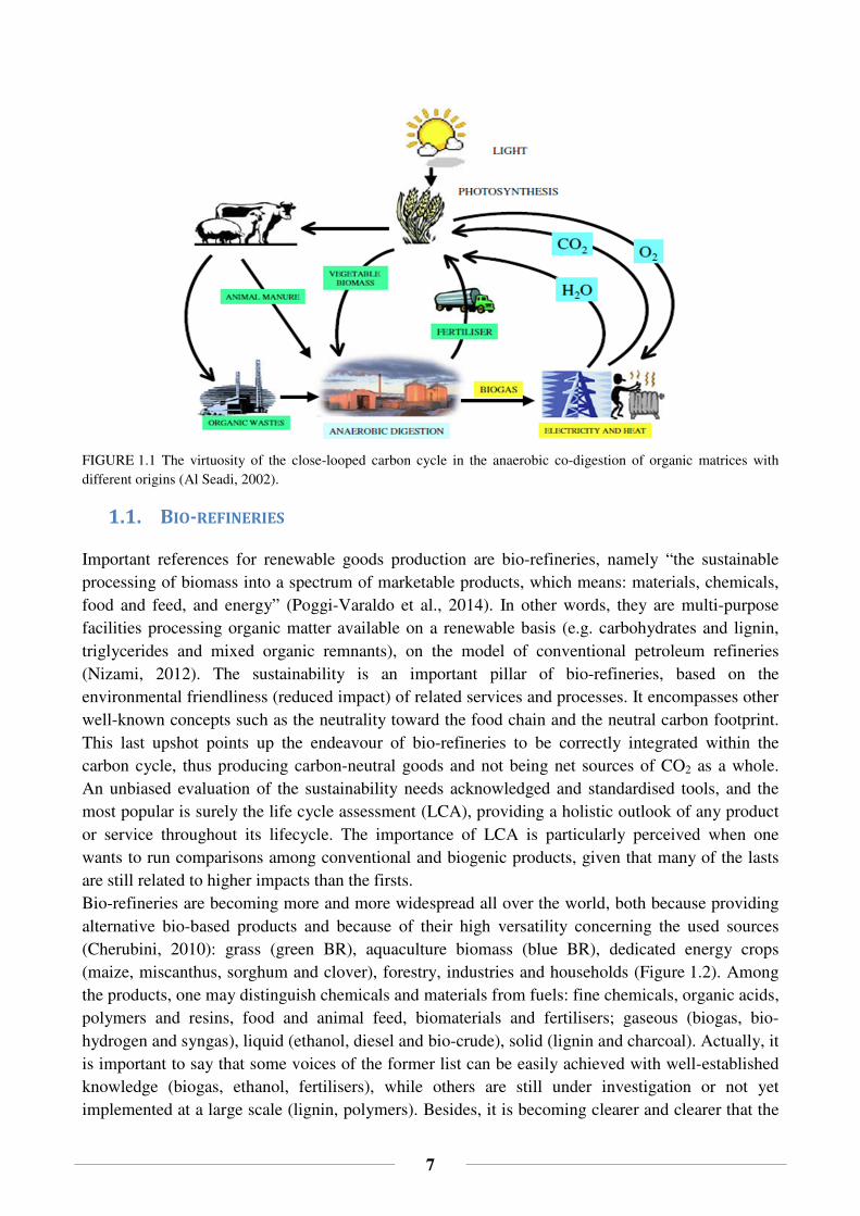
Anaerobic digestion (AD) is a biological process (bio-gasification) whereby consortia of microbes break the substrates down, generating a blend of gas (chiefly made of methane and carbon dioxide) from the organic load and a residual and stabilised solid fraction. It is a natural process occurring in many animals’ bowels (such as ruminants), as well as in the neighbourhoods of wet sites like swamps, wherein the appearance of flammable gas vents or bubbles was an early hint for the discovery and the study of the phenomenon from scientists like Lavoisier, Franklin, Priestley and Volta. The first and large-scale exploitation of AD was the sanitation of wastewater sludge at the beginning of the 20th century; then, thanks to progressive technologic adjustments, many potentialities of the process have been enforced, leading to the production of bio-methane and bio-hydrogen for heating, transport and energy purposes (combined cycle power plants), and digested matter as fertilisers for farming purposes (Figure 1.1). A noteworthy push to the development of AD technologies was the need of “green” and alternative destinations of organic waste both to landfills, severely limited by the European policies (i.e. Landfill Directive 1999/31/EC), and to thermal treatment (like direct combustion), unfeasible because of the high water content of some substrates. Biological treatment appears as the best solution, even if anaerobic digestion is considered more fruitful than aerobic composting, since the following reasons: higher recoverable energy (100-150 vs 30-35 kWh/Mg of waste); faster degradation rate, so smaller occupied areas; greater converted organic fraction, so more stable outcomes; limited quantity of process sludge and emissions of smells and greenhouse gasses, due to the fulfilment of the process inside reactors (Grosser et al. 2013). It is clear that it represents an easy and fruitful way to convert waste or biomass into green energy, even in comparison to other biofuels, like in terms of less water requirement (Al Seadi et al., 2008). AD was not much widespread till 1990, when the majority of organic waste was composted and disposed: a more and more growing environmental sensitivity has switched the scenario since then, and it is forecast that the 80% of waste will be anaerobically treated before 2020 (BMU 2005). Anaerobic digestion for the production of biogas may be carried out according to three fashions (Baromètre Biogaz, Eurobserv’er, 2012): landfills (passive), not advised, owing to the outdoor location and the ensuing low percentage of recoverable biogas (30-40%); urban wastewater and industrial effluents treatment plants; suitably designed energy conversion plants, dealing with a huge variety of waste (animal dung, agriculture products, food-processing, household organic fraction…). The main benefits coming from a massive employment of AD are: the avoidance of chemical and microbial contamination due to landfilled waste; the reduction of sludge volumes, organic content and dewatering difficulty; the cheap production of a useful high-energy bio-fuel which may replace the conventional fossil methane; the consequent ones; the possibility to sterilise digested substrates thanks to high temperature digestions; added value agricultural waste.

7

FIGURE 1.1 The virtuosity of the close-looped carbon cycle in the anaerobic co-digestion of organic matrices with different origins (Al Seadi, 2002).

1.1. BIO-REFINERIES

Important references for renewable goods production are bio-refineries, namely “the sustainable processing of biomass into a spectrum of marketable products, which means: materials, chemicals, food and feed, and energy” (Poggi-Varaldo et al., 2014). In other words, they are multi-purpose facilities processing organic matter available on a renewable basis (e.g. carbohydrates and lignin, triglycerides and mixed organic remnants), on the model of conventional petroleum refineries (Nizami, 2012). The sustainability is an important pillar of bio-refineries, based on the environmental friendliness (reduced impact) of related services and processes. It encompasses other well-known concepts such as the neutrality toward the food chain and the neutral carbon footprint. This last upshot points up the endeavour of bio-refineries to be correctly integrated within the carbon cycle, thus producing carbon-neutral goods and not being net sources of CO2 as a whole. An unbiased evaluation of the sustainability needs acknowledged and standardised tools, and the most popular is surely the life cycle assessment (LCA), providing a holistic outlook of any product or service throughout its lifecycle. The importance of LCA is particularly perceived when one wants to run comparisons among conventional and biogenic products, given that many of the lasts are still related to higher impacts than the firsts. Bio-refineries are becoming more and more widespread all over the world, both because providing alternative bio-based products and because of their high versatility concerning the used sources (Cherubini, 2010): grass (green BR), aquaculture biomass (blue BR), dedicated energy crops (maize, miscanthus, sorghum and clover), forestry, industries and households (Figure 1.2). Among the products, one may distinguish chemicals and materials from fuels: fine chemicals, organic acids, polymers and resins, food and animal feed, biomaterials and fertilisers; gaseous (biogas, bio-hydrogen and syngas), liquid (ethanol, diesel and bio-crude), solid (lignin and charcoal). Actually, it is important to say that some voices of the former list can be easily achieved with well-established knowledge (biogas, ethanol, fertilisers), while others are still under investigation or not yet implemented at a large scale (lignin, polymers). Besides, it is becoming clearer and clearer that the

8

enormous potential of microorganisms and their enzymes may be exploited by humans everywhere, rescuing, although partially, the national economy from oil price fluctuations. Despite the evocative potentialities, large-scale bio-refineries implementation is quite difficult, since it involves a radical change in people’s minds. For example, as the biomass transportation is a relevant cost, the way to optimise it is to increase the nutrients concentration of it. The second principle of bio-refineries is the cascading, whereby the improvement of sequencing processes dealing with an original amount of resource, allows a correct and full use of it. The direct cascading is a two-stage scheme where bio-products are stemmed before the bio-energy, whilst the inverse scheme adds an upstream bio-energy stage: the choice of the approach depends on the priorities of each Country, e.g. the inverse might be interesting for fossil fuels importers. An advanced development of the cascading is the industrial symbiosis, a virtuous framework able to fully valorise the inputs and to reduce emissions and waste streams: it involves the realisation of satellite industries processing the streams previously separated within the bio-refinery. As implicitly mentioned before, AD processes are run within bio-refineries, but it is even very important to highlight that high-quality and homogeneous substrates, like by-products of food industries, are not usually subjected to AD, because addressed to the withdrawal of components for noble and expensive bio-products with high market opportunities (food, cosmetics and pharmaceuticals). What is ordinarily sent to anaerobic digesters embraces any type of organic waste, like sludge from wastewater treatment plants, municipal solid waste (OFMSW), animal manure… Lignocellulose substrates cannot be yet correctly processed, owing to the high lignin content: yet, the EU renewable energy Directive ascribes twofold credits to the biofuels produced from them and from remnants. That huge variety of substrates allowed many Countries to produce biogas with different fashions: from advanced biogas plants, widespread all over Europe and United States, to small and local digesters fed with farming waste in developing Countries (India and China), where biogas mainly makes up to lighting and cooking. In the last years, the capacity of biogas plants rose from 25000 t/y in 1985 to the actual > 500000 t/y (Arsova et al., 2010), along with their rapid diffusion: for instance, over 120 new installations at European level were set in the decade 2001-2010 (Weiland, 2005). As shown in Figure 1.3, more than a half of the world’s biogas production comes from Germany and United States, thanks the setup of large-scale plants as well: one of them, “Klarsee” at Penkun, boasts an installed capacity > 20 MW, split up in 40 standard modules of 500 kW each one (EnviTec Biogas, 2006).

FIGURE 1.2 Scheme of a generic bio-refinery (Poggi-Varaldo et al., 2014).

9

FIGURE 1.3 Shares of biogas from the main producing Countries in 2008 (UNDP, 2012).

10

2. ANAEROBIC DIGESTION

By a biochemical point of view, anaerobic digestion is a type of microbial metabolism occurring in an oxygen-free environment. Many families of bacteria get the nutrients and the energy sources they need from a heterogeneous blend of substrates, producing a gaseous discharge, called biogas, whose likely composition is reported in the Table 2.1 and compared to the similar landfill and natural gases. The best stoichiometric model used for the forecast of the theoretic biogas and bio-methane production is the Buswell’s equation (formula 2.1), needing a first description of the substrate composition:

C�H�O�N� + 4a − b − 2c + 3d4 �H�O → 4a + b − 2c − 3d

8 �CH� + 4a − b − 2c + 3d8 � CO� + dNH� (2.1)

Along with it, the ultimate methane potential of a given solid substrate, described as a kind of thermodynamic limit (Shah, 2014), is an important quantity for the design of biogas plants. The really yielded biogas is indeed less, because of the use of a portion of substrate for the biomass growth and for the impossibility to degrade the whole input (15-20%). Average achievable results of the biogas production are reported in the Table 2.2 (48). It is important to state that biogas production is not constant over the time: it reaches a peak in the central stage of the process, being the upstream and the downstream ones remarkably scarcer. The extension of the process duration or retention time (RT) often favours a bulkier result achievement, which may compensate for the cost and the use of larger digesters and the process attendance.

TABLE 2.1 Composition of natural gas, biogas and landfill gas (Monnet, 2003 modified).

11

TABLE 2.2 Average yields of anaerobic digestion (Chaudhari et al., 2012).

Parameter Unit of measurement Average yield BOD removal % 80-90 COD removal mg/l 1.5 BOD Biogas production m3/kgCODremoval 0.5 Sludge production kg/kgCODremoval 0.05-0.1 Biogas production rate m3/kgVSdegraded 24-32 Heat value of biogas kWh/m3 6

The bio-methane fraction may have different applications, ranging from the early use as fuel in combined heat and power units (CHP) for the electricity independence of the plant, to the ensuing sale of the extra electricity or even the gas to suppliers. Before carrying the previous operations out, the biogas has to be purified, that is, deprived of those chemicals that unwanted side reactions of the AD process gave rise to and which may damage the working equipment (H2S, volatile siloxanes). Bio-methane is easily recoverable from the blend of digester matter, thanks to its negligible solubility in water; on the contrary, CO2 reaches a steadiness between the gaseous and the liquid phases.

2.1. RECALLS ON THE METABOLISM OF LIVING ORGANISMS

Each living organism is made of complicated structures of polymers, arranged together according to a well-defined fashion. The support of those very interesting configurations is possible only thanks to an external acquisition of energy and chemicals, whose transformations, favoured by organic catalysts (enzymes), are grouped in the metabolism. This various and multipurpose mechanism, allowing the growth and the reproduction of the organism, is the main topic studied by the biochemistry. Metabolism of chemotrophs, that is, those organisms whose energy sources are chemical compounds, inversely plants (phototrophs), is made of two complementary pathways. The catabolism is a convergent process that, starting from a huge variety of substrates, oxidises them back to easy compounds (often inorganic), with the production of energy, stored as high-energy bonds of devoted chemicals (like Adenosine-Tri/Di/Mono-Phosphate). On the contrary, the anabolism is divergent, since it takes and arranges simple external chemical structures up to the needed complicated ones, consuming a part of the formerly attained energy. The energy source may be either an organic (chemoorganotrophy) or an inorganic compound (chemolithotrophy), and in the same way the chemical source, mainly represented by carbon (heterotrophy and autotrophy). The energy that is rescued during the catabolism is embodied by an electrons flow moving from the oxidised source to the reduced final electron acceptor (FEA), which is another compound either external or internal (like in the fermentation) the cell. Therefore, it is clear that the amount of

yieldable energy (∆G0) is defined through a staged pathway of redox reactions. More in detail, each oxidation and reduction process is characterised by an electric potential, named redox potential E, whose negative difference between the reagents allows a thermodynamically feasible electrons movement. It is an indicator of the keenness of one substance to be reduced: the greater it, the better the compound as FEA, and the lesser it, the better the compound as electron donor. The relationship

between the produced energy and the variation of redox potential ∆E is linear:

∆�� = −��∆ (2.2)

12

Where n is the number of transferred moles and F = 9.648 × 104 C/mol is the Faraday constant. According to the identity of the FEA, one may have different types of respiration, like aerobic (oxygen), nitrate, sulphate or carbon dioxide, which are, of course, more or less energetic. That is very important, because the lower the rescued energy, the slower the cells activities (growth, reproduction) and therefore, the less competitive and “aggressive”. This is the context where the fermentation takes place: it is a particular type of anaerobic respiration where both the electron donor and the acceptor are products of the partial organic matter oxidation, chiefly the pyruvate. The oxidation of the substrates is carried out thanks to the massive intervention of coenzymes like NAD+ and NADP+: initially, they reduce by receiving electrons and couples of hydrogen atoms, and later they are regenerated by releasing the previous load to partially oxidised organic substrates. Fermentation involves each kind of substrate and it generally gives rise to acid and alcoholic yields, besides gaseous hydrogen; the most important fermentative process of the anaerobic digestion is the acidogenesis. The most used microorganisms are bacteria, the only class displaying a prokaryotic cell, which is smaller than the more developed eukaryotic one. The smaller size and the greater free surface/volume ratio are intuitive reasons why bacteria grow up faster than other microbes, since external nutrients are better caught and quicker metabolised inside the cell. Another key parameter is the diffusion, that is, the natural movement of substances from higher concentrations to lower ones; whence, the importance of fully dissolved substances within the liquid environment where cells live. Gaseous particles can easily spread in an out the cell across the membrane, while more complicated and larger ones (monomers) need the intervention of carriers for a driven (active) penetration; it needs energy in the form of ATP.

For a practical employment of the microbial communities, an apt mathematical description of their kinetics has to be shown. A short piece of the large literature written about that is reported in the follow-up. It is important to say that the reality may sensitivity divert from the available models although refined and proven; that is the reason why it is better to operate with a suitable confidence threshold. The first proposed kinetics concerns the cells (biomass) growth rate on a particular substrate, which is proportional to its consumption and it is rightly lessened by the natural cells death (or endogenous decay):

!"!# = $ !%!# − &'"

(2.3)

Where dX/dt and dS/dt are the biomass growth and the substrate consumption rates [M L-3 T-1], Y the growth yield [M generated biomass M used substrate

-1], kd the coefficient of microbial decay [T-1], and X the concentration of microorganisms [M L-3]. The second kinetics is the substrate consumption, which may be described with the theoretical model known as Michaelis-Menten equation:

!%!# = ()*+" %

(, + % (2.4)

Where Kmax the highest substrate consumption rate per unit mass of microorganisms [T-1], S the concentration of substrate [M L-3] and KS the coefficient of half-saturation [M L-3], which is the substrate concentration wherein the substrate consumption rate is the half of the maximum. Such formula explains that the highest consumption rate can be reached at an infinite substrate concentration, with a decreasing velocity of raise: that parameter is embodied by the slope of the

13

curve, which depends on the affinity between the biomass and the substrate and which is quantified by the coefficient KS (the greater it, the lower the affinity). By merging the former formulas, one may get a synthetic model, experimentally known as Monod equation, which can be further fit different circumstances, provided that the substrate is dissolved. In particular, when the substrate is plentiful (S >> KS), it can be traced back to a zero-order kinetic, while when the substrate is limited and KS significant, to a first-order one:

- = -)*+ %(, + % − &'

(2.5)

Where (µmax) µ is the (maximum) specific biomass growth rate [T-1]. Microbes working within anaerobic digesters may be liable to a poisoning due to an exceeding substrate concentration, and thus to an inhibition. The Monod equation can be modified so that to take this topic into account, with the introduction of coefficients of the inhibiting species:

- = -)*+ %(,(1 + 0/(2) + %

(2.6)

Where I is the concentration of the inhibiting substance [M L-3] and KI the related coefficient of half-saturation [M L-3]. An alternative approach is the first-order model, describing the substrate consumption over the time.

2.2. METHANOGENS

Methanogens may be fairly considered as the “engine” of the whole process, and that is the reason why in the follow-up a more careful characterisation of them is provided. They prefer living in low oxidation-reduction potential (ORP) environments, ranging between -0.4 and -0.2 V, where the presence of other final electron acceptors like O2, NO3

-, Fe3+ and SO4-- is limited: that is the reason

why they grow up more slowly than facultative and aerobic microbes. Nevertheless, they are usually found in mixed cultures, since other microbes can hydrolyse complicated polymeric chains otherwise unreachable by methanogens. Those cultures are easily traceable within many types of sludge, many animals’ bowels, anoxic sediments of deep water habitats, flooded soils for farming purposes (paddies), dump sites, geothermal and volcanic vents. Methanogens can be ranked in families according many factors, like morphology (shape and size), substrate specificity, optimal pH, optimal T, activator requirements.

2.2.1. Substrate specificity

Methanogens may be either facultative or obligate anaerobes, as well as either organotrophs or chemotrophs, according to the type of substrate where they pick nutrients up from. It has been assessed (Chaudhari et al., 2012) that in many ecosystems the 70-74% of methane stems from acetic acid thanks to the work of acetotrophic methanogens (acetoclasts), which cleave it into CO2 and CH4. Nevertheless, they are very sensitive to NH4

+ and H2 concentration rise, which is paid in terms of reproduction slowing. The strategy to keep them active is the support of hydrogenotropic activity, able to consume H2 and to establish a good (low) partial hydrogen pressure within the digester (10-3-10-5 atm); in the meanwhile, acetogens work and therefore acetate production is favoured as well. According to the previous reference, a 30-33% of methane is produced by

14

hydrogenotropic methanogens from the joint oxidation of H2 and reduction of CO2, which plays the role of carbon source and which can be retrieved from the cleavage of acetate as well. Some of them reach the target with the use carbon monoxide and water. For each produced mole of CH4, one ATP is generated too. The last and very widespread family of methanogens are the methylotrophs, which use the methyl group (–CH3) held within many compounds like methanol and methylamines.

As mentioned at the beginning of the paragraph, a correct AD process is based on delicate steadiness among microbial communities and that is maybe more evident after the analysis of methanogens. As a matter of fact, they live off and remove the products of the acetogenesis, whose accumulation would poison and inhibit the same ones (H2). Besides, methanogens could not be fed by the VFAs and alcohols directly. This peculiar biological circumstance is referred to as syntrophy, meaning “nourishment together”: a malfunction of methanogens triggers the failure of the whole digestion, which ends with an uncontrollable accumulation of acid yields. It was proven that the remarkable drawbacks of the previous result are the generation of stressing conditions for methanogens, which brings to their activity inhibition (deterioration), with difficulty restored. Syntrophic acetogens process is known as β-oxidation and it consists in the oxidation of both even and odd carbon number VFAs into H2, propionic and acetic acid; later, propionic acid undergoes a decarboxylation which gives rise to CO2, H2 and acetate.

2.2.2. pH

The pH is an important parameter which sets the correct development of the process. The best conditions are granted within a very narrow pH range (7.2-8.2), but half degree of tolerance can be stood. The pH is often affected by countless reactions producing acid and basic compounds, as well as by the buffer effect of some chemicals (e.g. ammonium bicarbonate NH4HCO3); some knowledge about reactions dynamics is important for the identification of those substances responsible of inhibition effects. Therefore, if VFAs, the most harmful of which are propionate and butyrate, are often neutralised by ammonia, excessive concentrations of the last one could not be aptly offset, with the ensuing pH rise. By a biological point of view, during the methanogenesis, a pH range (6-8) allows a fair trans-membrane movement and consequent absorption of not-dissociated acetate (CH3COOH) by methanogens, because of presence of a suitable concentration gradient. Besides being lethal for methanogens, lower values generate a huge availability of not-dissociated acetate, whose uncontrolled ingress within the cell becomes no more sustainable for it, leading to a substrate inhibition. Inversely, higher values provoke a widespread dissociation of acetate and the concentration of the non-dissociated form is no more enough to run the previous catabolism.

2.2.3. Temperature

Each kind of microorganism (methanogens too) displays its best growth performances within a usually narrow range of temperature. Since a fair variation of it leads to a sharp change of the microbial community diversity, it is particularly easy to rank microbes according to their favoured temperature conditions: psychrophilic (< 20°C), with the optimal conditions in the interval 15-20°C; mesophilic (20-45°C), with the peak in the interval 30-38°C; thermophilic (up to 70°C), with the peak in the interval 47-57°C. Temperature affects the generation time as well: from 3 days at 35°C up to 50 days at 10°C. Up to now, the majority of anaerobic digesters were planned for

15

mesophilic conditions, because more naturally plentiful in the digested substrates, thus not needing a further “sowing” or “bio-augmentation” (Schanbacher, 2009). Notwithstanding, thermophilic microbes are becoming more and more widespread, as higher temperatures allow a complete death of pathogens and a quicker methanogens growth, getting the overall process more efficient and faster (lower HRT), and therefore more fruitful. On the other hand, thermophilic microorganisms dreadfully suffer from small temperature variations, needing a long restoration period, as well as the temperature preservation could become a relevant cost. Their employment in the production of bio-hydrogen was proved particularly satisfactory (Schröder et al., 1994), reaching the theoretical stoichiometric yield of 4 mol/mol of glucose. Mesophilic microbes can bear fluctuations till ±3°C, without sharp reduction in the methane yield, hence allowing a more flexible reactor management. Despite the methane yield form psychrophilic microbes’ activity is comparable and more stable than the one from mesophilic ones, the large size of the fermenters due to the slowness of the process imposes notably expensive and unprofitable investments. As a matter of fact, low temperatures involve the slowing down of many enzymatic and biological activities (transcription, translation, cell division), the formation of ice within the cell, the protein impairment and the decrease of the membrane fluidity. The most popular way to assess the speed variation of a generic reaction kinetic due to the temperature is the Arrhenius equation:

45 = 4�67(5859) (2.7)

Where vT and v0 are the reaction rates at a given temperature T and at a reference T0, while φ is an experimental coefficient, normally constant within the temperature ranges of the reactors.

2.2.4. Toxic elements

It is important to remember that methanogens are the weakest microbial community of the whole AD process and particularly prone to substrate inhibitions. The chief inhibiting substrates are the VFAs (propionate) and acetate, whose uncontrolled accumulation provokes additional damage for the consequent pH lowering. Oxygen cannot be minimally stood by methanogens (conc?), although it can by the other microbes of the consortium, which are facultative. The skill of a microorganism to bear oxygen concentrations hinges on the synthesis of enzymes (i.e. superoxide dismutase and catalase) able to trace reactive oxygen species (ROS) back to harmless compounds. For example, H2O2 and O2

- are ordinary and very reactive by-products of the aerobic respiration, which could be generated by anaerobes using O2, but without being later cancelled. As far as external chemicals are concerned, they may induce different answers from methanogens. Sulphuric acid is an indicator of SRBs activity which, on one hand compete with methanogens for the substrate, on the other hand increase H2S concentration, that cannot be stood beyond 1000 mg/kgTS even if stern damage is perceived at 200 (optimal 8-22). Ammonia concentration is ordinarily borne up to 1500 mg/kgTS and inhibitory beyond 3000: for intermediate values, it depends on the adaptation skill of the methanogens, but generally those concentrations are bearable when pH > 7.4. In addition, ammonia toxicity grows with the temperature, and that might make thermophilic microbes more liable to this type of inhibition than mesophilic ones. Notwithstanding, ammonia concentration raise is along with VFAs one (Weiland, 2010), which partially neutralise each other. Even salty environments are harmful (the limit is 500 mM) and they favour the accumulation of fatty acids with the consequent drawback of pH decrease. On the contrary, some organic substances, like phenol and formaldehyde, can be degraded to methane when their concentration does not exceed a stated threshold (2000 and

16

400 mg/l). Although detergents (soaps), antibiotics and organic solvents inhibit microbial activities, sometimes methanogens may be enhanced after an utter early contamination operated by them (e.g. chloroform), becoming able to withstand higher concentration of polluting substances. It is possible to contain these types of poisoning by dilution below the toxicity threshold with water or process effluents (Shah, 2014). Finally, high heavy metals concentrations are dangerous for many bacterial activities since they can suddenly react with the sulphide group of many enzymes, destroying them and generating an insoluble compound. Once retrieved its respective solubility, it is clear that knowledge about S anions concentration lets one infer the metal cations ones. Therefore, one may assess the excess or not of the bearable threshold concentration (Table 2.3), which provokes several problems like the sensitive fall of fatty acids production and, thus, methane.

TABLE 2.3 Toxicity thresholds of some occurring metals (Cecchi et al., 2005).

Element Toxicity threshold (mg/l) Zinc 160 Copper 170 Chromium and cadmium 180

2.2.5. Habitats

Moving toward a chemical characterisation of methanogens habitats, anoxia is the most important condition to be respected. Sediments of deep aquatic environments are a good place, since their stillness prevents oxygen from recirculating. In the same way the saturated zone, which is the portion of soil beneath the water table, while the unsaturated one above may seldom be the seat of anaerobic habitats (named anoxic pockets). It is even possible to have methanogens activities in aerobic environments: it is the case of particular conditions where aerobic microbes induce anoxia by picking oxygen up or where the arrival of a small quantity of pollutant quickly pulls the available oxygen down. As aforesaid, a right concentration of final electron acceptors related to high ORP conditions inhibits methanogens work: that is due to several advantages the in charge microbes have got with respect to methanogens. As far as the chemolithotrophic metabolism is concerned, nutrients concentrations (like H2) for methanogens should be greater than 5, while lower for the other (e.g. 1-4 for sulphate reducing bacteria, SRBs). Besides, chemoorganotrophic non-methanogens produce much energy, with the consequent faster growth rate and substrate depletion, penalising methanogens. In particular, plentiful SRBs prevent each type of methanogenic conversions, but the ones based on methylated compounds, like tri-methylamine and di-methyl sulphide, frequently occurring within marine sediments. A scarce sulphidogens presence may allow methanogens activity and the best indicator thereof is the study of the fate of the methyl group belonging to acetate: if it is converted into CH4 rather than CO2, methanogens start prevailing. Nitrogen containing compounds are essential for the cells life, but many Archaea can even dwell in nitrate-rich habitats, especially the most extreme ones, where they actually contribute to the nitrogen cycle by reducing nitrate to N2 thanks to organic substrates.

2.3. STAGES OF THE ANAEROBIC DIGESTION

Anaerobic digestion is a process which may be accomplished only thanks to a mutual and serial collaboration of many microbial families (microbial web or chain) with deeply different earmarks and growth parameters among them (Table 2.4). The products of the chemical conversion by one

17

community become the starting point for the next one, up to the last step which is carried out by methanogens. Generally, one may argue the existence of four chief and simultaneous microbial/enzymatic stages, explained in the follow-up and summarised in the Figure 2.1. It is important to say that each process has got its own optimal operative parameters and thereby an overall appraisal is not feasible.

TABLE 2.4 Staple microbes involved in the anaerobic digestion (Abbasi et al., 2012).

FIGURE 2.1 Scheme of the four phases of the AD and involved substances (modified from Cecchi et al., 2005).

18

2.3.1. Hydrolysis

Hydrolysis is a biologic lytic process whereby the polymers (lipids, polysaccharides and proteins) which the substrate is made of are degraded back to the original and water-soluble “building blocks”, that is, oligomers and monomers: long-chain fatty acids, monosaccharides and amino-acids. Each of them, as reported in Table 2.5, has a different yield of biogas and methane: in particular, fats are the most fruitful, due to already available VFAs, while proteins can return the most methane-rich biogas. That operation is performed by aerobic and anaerobic hydrolytic microbes yielding extracellular enzymes. Anyhow, that enzymatic activity may be deeply impaired by an uncontrollable accumulation of amino acids and saccharides. Quantities of H2 can be produced, e.g. from the cleavage of the adipic acid, like shown below:

C:H;�O� + 2H�O → C:H;�O: + 2H� (2.8)

lipids @AB�CDEFFG fattyacids, glycerol proteins BQRSD�CDEFFFFFGaminoacids

polysaccharides �D@@V@�CD,�D@@R�A�CD,WX@�Y�CD,�ZX@�CDEFFFFFFFFFFFFFFFFFFFFFFFFFFFGmonosaccharides TABLE 2.5 The potentialities of biogas and methane production from different elementary monomers (Weiland, 2010; Baserga, 1998).

Substrate Biogas (Nm3/MgTS) CH4/CO2 Raw fats 1200-1250 ≈67/33 Raw proteins 700 ≈70/33 Carbohydrates (but inulins and single hexoses) 790-800 1/1 Lignin 0 Both zero

Hydrolysis is the limiting stage of the whole AD, because of the huge variety and complexity of organic matrices to be degraded (e.g. cellulose), as well as pH, temperature and particles size: that makes the process modelling quite uncertain. The reliable model proposed by Eastman and Ferguson (1981), based on a careful choice of coefficients and on a first-order kinetic, independent of the concentration of hydrolysing microbes, is reported beneath:

[\, = −(% (2.9)

Where RXS is the specific hydrolysis rate [M L-3 T-1] and K the maximum specific hydrolysis rate [T-

1]. The values of K hinge on the type of substrate: lipids (0.1.0.7 d-1), proteins (0.25-0.8 d-1) and carbohydrates (0.5-2 d-1).

2.3.2. Acidogenesis

Acidogenesis is the main fermentative stage where the blend of mono and oligomers is converted into hydrogen, CO2, acetate, alcohols, ketones and low molecular weight volatile fatty acids VFAs (lactate, propionate and butyrate chiefly) by extracellular enzymes producing bacteria, some of which ran the previous step as well. Side fermentations of amino acids give rise to other by-products as well, like CO2, NH3 and H2S, whose permanence within the digestates constrains some apt treatment (oxidation) before their sale as soil enricher.

19

C:H;�O: + 2H� → 2CH�CH�COOH + 2H�O(butyricacidfermentation) (2.10)

C:H;�O: → 2CH�CH�OH + 2CO�(alcoholicfermentation) (2.11)

CH�COOH + SO��8 → 2HCO�8 + H�S (2.12)

CH�COOH + H�O + NO8 → 2HCO�8 + NH�_ (2.13)

The acidogenesis is properly defined as a dark fermentation, opposed to the photo-fermentation, since it does not need natural or artificial light. It can be finally described by the Monod equation (Formula 2.5), being careful in the choice of the substrate concentration, changing with the considered monomer. Suggests values from the literature are (Eastman and Ferguson, 1981): µmax=3-9 d-1; Kmax=24-120 gCOD/gCOD/d; KS=300-1400 mgCOD/l; Y=0.01-0.06 gVS/gCOD; kd=0.02-0.3 d-1.

2.3.3. Acetogenesis

Acetogenesis is run by facultative and obligate hydrogen-producing acetogens, which oxidise fatty acids into mainly acetate (51%), H2 + CO2 (19%) and formic acid (Formulas 2.14-2.16). That operation, by a theoretical point of view, is thermodynamically disfavoured, as well as inhibited by a high H2 partial pressure; it becomes really feasible thanks to the presence of H2 oxidising microbes (methanogens). It can be studied with a Monod model similar to the precedent, with a significant distinction between LCFAs and VFAs during the choice of the coefficients (Table 2.6).

CH�CH�COOH + 3H�O → CH�COOH + H�CO� + 2H� (2.14)

CH�CH�OH + 2H�O → CH�COOH + 2H� (2.15)

2H�CO� + 4H� → CH�COOH + 4H�O (2.16)

TABLE 2.6 Coefficients for the different types of fatty acids (Cecchi et al., 2005).

µmax (d-1) Kmax (gCOD/gCOD/d) KS (mgCOD/l) Y (gVS/gCOD) kd (d

-1) VFA 0.3-1.3 5-20 100-4000 0.02-0.07 0.01-0.04 LCFA 0.1-0.5 2-20 100-4000 0.04-0.1 0.01

2.3.4. Methanogenesis

Methanogenesis is a broad family of reactions carried out by methanogens (Archaea bacteria), giving rise to methane from the three main products of the former stage (Formulas 2.17-2.19). A correct AD progress involves the equivalence between the degradation rate of the methanation and of the upstream processes: it is evident that a too much rapid development of the last ones lowers the pH below 7.0, inhibiting the methanation.

CH�COOH → CH� + CO� (2.17)

CH�OH + H� → CH� + H�O (2.18)

CO� + 4H� → CH� + 2H�O (2.19)

20

Kinetics is usually represented with the Monod equation with the substrate inhibition. The formula 2.6 can be applied for methylotrops and acetothrops, while hydrogenotrops need a model with two inhibiting substrates S1 (hydrogen) and S2 (carbon dioxide):

- = -)*+ %;(,; + %;

%�(,� + %�

(2.20)

Methane is rightly assumed as the last outcome of the whole AD, because of its lack of reactivity and its low solubility in the water phase, which contributes to its removal from the system and to the difficulty to take part to further biologic processes. It is important to state that, regardless of the whole process is referred to as anaerobic, the only strictly anaerobic stage is the methanogenesis: the upstream ones can be run by both anaerobic and facultative bacteria. Some author (Davis and Cornwell, 1998) argues that it is the limiting stage of the chain, thus conflicting with the former statement. Generally, one may say that the most relevant constraint of hydrolysis is represented by cellulose and large particles size, therefore by substrate and pre-treatment issues. By a design viewpoint, since the kinetics of the slowest route is crucial for the whole process, one might advise single-stage fermentations when hydrolysis is not constrained and two-stage ones otherwise.

21

3. INDUSTRIAL PROCESS

The purpose of this chapter is to explain the staple standards for the large-scale implementation of anaerobic digestion, besides to show the most optimised types of process which are presently on the market, along with several pilot-scale applications.

Industrial-scale anaerobic digestion is usually carried out within suitable vessels (or digesters), sometimes belonging to more complicated facilities named biogas plants. Their shape, the number of needed steps (single or multi-stage systems), the presence of pre-treatment, as well as careful controls over operational parameters can tightly affect the biogas production yield. The design of anaerobic digesters must take into account not only the achievement of stable thermodynamic equilibria of the reactions, but the operating costs as well, which might not be offset by a consequent greater yield. This is why the design approach is usually based on the reaction speeds (kinetic). According to that strategy, one has to consider two types of complementary microbiological kinetics, explained in the former paragraph: the biomass growth speed on a substrate and the substrate consumption, described with both the Michaelis-Menten and the Monod equation (formulas 2.4 and 2.5).

3.1. SUBSTRATE CHARACTERISATION

As well as the design parameters, the biogas production is severely affected by the substrate type and composition (Zaher et al., 2007); Table 3.1 reports the methane yield of some AD experiences carried out with different substrates. Macronutrients such as carbon, nitrogen, phosphorous and sulphur are needed in short amounts indeed, since the limited development to biomass, but according to a well-established proportion (C:N:P:S = 600:15:5:1). It is important to point up that higher carbon concentrations provoke a short cellular synthesis of basic polymers, whilst lesser ones could give rise to inhibition issues (e.g. ammonia and hydrogen sulphide). Micronutrients are embodied by metals like iron, nickel, cobalt, selenium, molybdenum and wolfram which build some important enzymes and which have to be added to those substrates short in them (e.g. energy crops). As aforesaid, micronutrients might inhibit microbes, and that is the reason why a strict control over their concentration is needed: 0.05-0.06 mg/l, but the iron, which has to reach 1-10 mg/l. The substrate characterisation is an as essential as difficult topic, owing to the previously hinted heterogeneity; that is the reason why global parameters are preferred to thorough and diverting chemical analyses. Total solids (TS) are the mass of substrate after drying treatment at 105°C for 24 h; it may be considered as the sum of organic and inorganic matter. That parameter can remarkably vary, defining the type of digestion (wet, semi-dry or dry); generally, it does not get 40% in mass over, so that to allow an easy agitation and biogas stripping. Total volatile solids (TVS) represent the mass of TS rescued for oxidation at 550°C and which roughly embodies the organic fraction of the TS; similarly, the residue, called total fixed solids (TFS), embodies the inorganic

22

fraction. Finally, the chemical and the biological oxygen demand (COD and BOD) are two very popular characterisations in health engineering. They represent the overall need of O2 for the oxidation of an organic substrate, in the first case, chemically (with K2Cr2O7) and within an acid environment, while in the second case biologically and after five (BOD5) or twenty days (BOD0).

TABLE 3.1 Methane yields of several raw substrates (Grosser et al., 2013).

Substrate Methane yield (m3/kgVS) Fruit and vegetable waste 0.42 Grease trap sludge 0.85-0.93 Household waste 0.35 MSW 0.36 OFMSW 0.38 Pig manure 0.20-0.30 Raw glycerol (biodiesel production) 0.69-0.72 Sewage sludge 0.26-0.46 Source-sorted OFMSF 0.28-0.41 Swine manure 0.34

3.1.1. Co-digestion

It is important to say that some families of substrates may result inadequate on their own for a successful AD, since the low amount or an incorrect partition of essential nutrients. Key examples are the carbon-to-nitrogen ratio, the amount of biodegradable matter, the pH, the presence of inhibiting substances and the quantity of microbes, micro and macronutrients. An interesting way to improve the biogas production by working on the substrate is the co-digestion, properly “the simultaneous anaerobic digestion of a homogeneous mixture of at least two components” (Del Borghi et al., 1999). Co-digestion is realised simply by merging different waste streams among them, like: industrial waste streams (e.g. slaughterhouse waste, food remnants), sewage sludge, animal manure (rich in bacteria, water and nitrogen…); OFMSW, agriculture leftovers, crude glycerol (rich in carbohydrates, fats…). It is clear that this strategy offers the noteworthy opportunity to solve many waste management problems at once, giving rise to broader and more optimised chances otherwise inaccessible by the single streams separately. The most popular co-digestion strategy blends a main stream with smaller ones having quite opposite earmarks, so reaching the desired nutrients and microbes balance. That has been proven by plentiful experiences carried out with OFMSW and WWTP sludge: as benefits one may claim the increased biogas yield and the methane content, the higher conversion of the organic fraction, the buffer capacity of some damaging earmarks (pH, toxic substances) and the adjustment of some lacks like nutrients and moisture. Other notable examples are the use of uneatable oilcakes for the C/N ratio adjustment (Lingaiah and Rajasekaran, 1986), and the combined use of chicken dung and fruit leftovers, able to fight the ammonia inhibition triggered by the previous one and to raise the bio-methane conversion (Callaghan et al., 2002). Co-digestion is also related to drawbacks such as the difficulty of conveying many streams toward a central treatment plant, the low quality of the reactors effluents and the need of advanced pre-treatment (Nayono, 2009; Bien et al., 2010). The last aspect is compulsory for industrial waste streams, so much so that the higher biogas yield (12.7 GJ/MgDM from food remnants against 5.9 GJ/MgDM from cattle manure, according to Pöeschl et al., 2010a) is often not preferred to the higher costs of sterilisation.

23

3.1.2. Energy crops

The name energy crops points out a broad family of vegetable biomass which are purposely grown and harvested for the conversion into renewable energy sources. They, and in particular corn, occupy a relevant share in the world’s biogas production, so much so that the whole yearly European feedstock from agriculture (1500 millions of tonnes) is in half made of them. Moreover, it is important to highlight that they may valorise wide surrendered fields, generating job opportunities and economic growth for the export of the technology (Pöeschl et al., 2010b). Energy crops can be harvested up to eight times per year, distinguished according to the season: for instance, maize in the summertime and rye in the wintertime (Jury et al., 2010). Perennial and spontaneous grass (e.g. rye grass in Ireland) is often associated to energy crops, regardless of the cheapness. Along with their more and more rapid diffusion, these crops arouse ethical discussions about the subtraction of resources and land to the food stream (e.g. 21560 km2 of German soil in 2012). Other negative aspects concern the expensiveness of the intensive cultivation process, (1.87 €/Mg according to Pöeschl et al., 2010b), the dependence of market swinging (price, availability and logistics) and to government subsidies, as well as the soil detriment due to the deployment of monocultures (mainly corn and grass). Table 3.2 reports the most common types of plants used within energy crops and their average efficiency of production.

TABLE 3.2 Methane yields per unit of cultivated surface and per kg of VS (Appels et al., 2011; Shah, 2014).

Name Methane yield (m3/ha) Methane yield (m3/kgVS) Grass 3100-5000 0.42 Maize 8100-14000 0.36 Sorghum 6300-14000 0.37 Sugar beet 3600-6600 0.34 Sunflower 2100-3800 0.30 Triticale 7000-9000 0.49 Wheat (grain) 1900-3400 0.45

They may be digested alone, but careful controls have to be carried out over mostly the micronutrients availability. The main advantage of the alone digestion is the high nitrate content within the solid digestate, up to threefold the average one (Shah, 2014). Otherwise, they are co-digested along with manure, where high energy content meets the wanted moisture and bacterial load: in particular, Browne et al. (2011) suggest a ratio 3:2 for grass and animal slurry. Once harvested, energy crops undergo a kind of pre-treatment consisting in shredding (till d = 10-20 mm) and storage inside silos, where it is covered with a protecting plastic wrap and watered up to an optimal solid content between 25% and 35%. There, the carbohydrates oxidise to lactic, propionic, butyric and acetic acids, with the ensuing pH fall (3-4); the digestion often becomes more difficult owing to the matter prone to float. The partial loss of the energy content (8-20%) is offset by the successful killing of harmful microbes. Then, the slurry should have the right earmarks to be pumped within the fermenters, where the AD takes place; usually, the wet is the most used process, with low solid concentration (2-4%) and high retention times (weeks to months). Sometimes, two-stage and dry batch processes are preferred (up to 70% of solids): the first ones with the aforesaid peculiar configuration, while the second one with durations comparable to the wet processes.

24

3.1.3. Animal by-products

Animal manure is another type of feedstock, known as a mixture of slurry urine, faeces, water and bedding material coming from the breeding of cattle (chiefly bovine and pig). The management of such materials is becoming more and more important worldwide, since it is a proven cause of chemical and microbial contamination, but even a stabiliser of the AD process and a source of minerals for the ensuing use of the digestate as fertiliser in the farming sector (65% in Europe, according to Menzi, 2002). For instance, outdoor manure heaps not only generate nuisance from smells and bugs, but they release widespread vents of dangerous GHGs such as ammonia and methane, whose global warming potential (GWP) is up to 21 times the one of CO2. According to Steinfeld et al. (2006), the breeding sector is responsible of the 18% of the global GHGs emissions (in terms of CO2-equivalent) and of the 37%, 64% and 65% of anthropogenic pollution of CH4, N2O and NH3. In this contest, the AD in a co-digestion scheme, besides without any need of pre-treatment, can play a significant role in the reduction of pollution and in the valorisation of what is generally regarded to as troubling waste; furthermore, it may become an economical benefit for farmers. Møller et al. (2009) appraised that the GWP of a biogas plant ranges between -95 and -4 kgCO2eq/Mgwet waste, thus an evident benefit, though with large uncertainties due to fugitive CH4 vents and CO2 sequestration (e.g. the solid bio-char as soil amendment). Slaughterhouse waste (SHW) is attracting much interest as biogas substrate, since the huge production and problems in the management: bowels, offal and wastewaters can be easily addressed to AD processes, while animal proteins and fats arouse the interest from biodiesel producers.

3.2. REACTOR PARAMETERS

The reactor structural design is a complicated procedure which has to match up physical and biological aspects and which can return different process and plant configurations. In the follow-up, the two families of parameters used for that fulfilment are explained.

Reactor management parameters describe the more physical aspects of the process, related to hydraulics, composition and dimensions (Cecchi et al., 2005). The hydraulic retention time (HRT) is the ratio between the vessel volume V and the incoming feed rate Q and it represents the duration of the stay of any type of fluid particle within the vessel. It is an average value, because it may be greater or lower, according to the type and the shape of the reactor. It is also referred to as volumetric loading, opposed to the mass (or digester) loading, which is related to the organic concentration of the influent. Similarly, the sludge (or solid) retention time (SRT) is a mean quantity defined as the ratio between the mass of the volatile fraction within the reactor and its removal rate from it or, in other words, it is the period the microbial biomass spends inside the vessel.

%[` = a"b

(3.1)

Where X is the concentration of VS inside the reactor [M L-3] and W the outgoing flow of VS from the reactor [M T-1]. Steady-state conditions can be reached when the amount of biomass within the basin is constant, that is, the removed levels the generated one. The ratio between the previous times is the controlling factor of any biological treatment: it is also referred to as “food to microorganism ratio” (F/M) and it should be kept as lower as possible, e.g. increasing HRT and decreasing SRT by preserving the biomass. The organic loading rate (OLR) is the flow of organic

25

matter entering the system per unit of useful vessel volume. It can be considered as the threshold volatile matter quantity that the system can stand: an excess of it rapidly causes VFAs accumulation and pH lessening:

cd[ = e%a

(3.2)

Where S is the substrate concentration in the incoming flow [M L-3]; the numerator can be replaced with other estimates such as TS or COD. The charge factor (CF) is a similar concept, but it is referred to (divided by) the unit of volatile solids within the vessel X: the main weakness of that parameter is the difficult distinction between substrate and biomass over the total organic fraction. The former list of parameters crucially defines an important distinction among digesters, the low-rate and the high-rate ones: a more detailed study will be reported later. The specific gas production (SGP) is the volume of produced biogas per unit of entering volatile mass. Although it is mainly used for the process yield assessment, instead it crucially depends on the substrate properties:

%�f = eghij*ke%

(3.3)

The methane yield is a quantity that can be inferred from the SGP by knowing the percentage of CH4 over the total biogas, which is broadly changeable (40-70%), but normally in the range 55-65%. An acceptable estimate of the highest theoretical methane yield is roughly 0.5 m3/kgVS (Browne et al., 2011), based on the assumption that the energy content of one tonne of VS (HHV = 19 GJ) is utterly converted into methane (HHV = 38 MJ). The gas production rate (GPR) is the ratio between the generated biogas flow Qbiogas and the vessel volume. The substrate removal efficiency η represents the bounty of the process in the mineralisation of the organic fraction:

l = e% − e%me% = 1 − %m

% (3.4)

Where Se is the concentration of VS in the outgoing flow [M L-3], which can be inferred as difference between the incoming mass and the amount of produced biogas, or computed with some knowledge about the volatile content of the influents and effluents.

Design models based on the Michaelis-Menten equation rely on the variable S and the constant Kmax (or k in first-order kinetics), stemming from a global characterisation of the substrate (lipids, proteins and polysaccharides); despite the easiness, it is quite difficult to assess S reasonably, unless with rough estimates (COD). That is the reason why it is preferred to shift the analysis on the biogas yield at infinite time (also called maximum biogas conversion potential) of a given substrate, B0, appraised with the Chen and Hashimoto’s formula:

n� − nn� = %

%� (3.5)

Where the subscript 0 refers to the quantities at an “infinite” time. It is a general indicative equation that cannot be solved as it is, but it has to be fit the different circumstances, for example the continuous stirred-tank reactor (CSTR) through the mass balance:

26

e%� − e% − &a% = 0 → %%� =

ee + &a = 1

1 + &p[` (3.6)

Then, the values of k and B0 can be achieved by drawing a regression among couples (HRT, B). This model may avail when the complexity of the treated organic substrates does not allow a stoichiometric biogas forecast with the aforementioned Buswell’s equation.

On the contrary, process stability parameters explain those topics whose incorrect handling could sternly impair the microbial activities and chiefly the methanogenesis. It is important to mention that the correct preservation of these quantities needs a thorough monitoring system and only through a simultaneous comparison among freakish data it is possible to identify malfunctions. The alkalinity (or total inorganic carbonate) is the buffer ability of the system, that is, to take protons up. It is usually measured in terms of CaCO3 concentration through titration with HCl, and ordinary values range between 3000-5000 mg/l. The alkalinity plays a relevant role in the whole AD when a massive entrance of substrate prods an uncontrollable development of hydrolytic and acidogenic activities and growth, with the consequent pH fall. The combined work of bicarbonate and ammonium, respectively stemming from the CO2 solubilisation and the amino acids degradation, gives rise to the salt NH4HCO3, able to buffer acid imbalances according to the reactions:

CO� + H�O → HCO�8 + H_ (3.7)

R − NH� → NH�_ + HCO�8 + xCO� + yH�O (3.8)

HCO�8 + NH�_ → NH�HCO� (3.9)

Factors which the pH hinges on are represented by the concentration of some chemicals in the liquid phase, like fatty acids, ammonium and CO2, as well as by the partial pressure in the biogas of the last one. It is then clear that the stability of the process, met when the pH is close to the basicity (6.5-7.5), can be granted through the efficiency of a buffer system. When this one is no more efficient and pH carries on decreasing, it is possible to neutralise the environment with the addition of lime (CaCO3). The control over the pH is a relevant example of the aforesaid integrated monitoring of different quantities: as a matter of fact, it cannot return reliable information about process imbalances occurrence in and of itself (e.g. acidification), since the buffer system restrains its variations (Figure 3.1).

FIGURE 3.1 Buffer effect of the system and delay of the pH drop with respect to the alkalinity (Cecchi et al., 2005).

27

This is the reason why more important hints can be achieved from VFAs concentration and biogas composition trends. Optimal VFAs concentration in the digester, reckoned as acetate or more seldom as COD, should drop between 200 and 2000 mg/l, but actually more interesting information are provided by sudden variations of it. A good approximation of this parameter is reachable through the liquid mean titration with HCl: in particular, through the difference between the alkalinity at pH=6, corresponding to the depletion of the buffering skills, and at pH=4. Several authors (Nielsen et al., 2007) propose sterner controls over the propionate so that to identify reliable incoming process failures. In particular, not only the concentration on its own, but also a ratio with the acetic acid greater than 1 is an indicator of instability; furthermore, butyrate and iso-butyrate concentrations become reliable gauges when the one of propionate gets 1000 mg/l over. It is even possible to merge VFAs concentration and alkalinity in a unique ratio which represents stable conditions around 0.3. Three proposed sceneries over the time (Cecchi et al., 2005) on biogas composition and quantity can be reliable indicators of the progress development as well. Stability is embodied by a constant and plentiful biogas production and low CO2 percentages (25-33); inversely, VFAs concentration raise may be ascribed either to inhibitions and poisonings, when the biogas production decreases, or to a gradual prevalence of acidogenesis, when CO2 concentration rises (up to 67%). Hydrogen presence control within the biogas is another significant tool at a laboratory scale, but not yet applied to industrial realities, since the low amount of it. The sensitive affinity of each microbial community with a narrow temperature range induces a careful control over the heating system of the plant. One may work under mesophilic (30-38°C) as well as thermophilic conditions (47-57°C), being aware that the greater the temperature, the less stable but the smaller the reactor (and conversely), as aforementioned. Actually, as the biogas production (but not the methane yield) increases with the temperature inside the range, one is interested in working with threshold values and that can become a demanding requirement.

3.3. CONTINUITY IN SINGLE-STAGE PROCESSES

As mentioned at the beginning of the section, a key role in the correct progress of the digestion is played by the configuration of the reactors and the number of stages. In single-stage fermentations, the digestion as a whole takes place in one vessel, therefore the structural design will be carried out according to the times of the methanogenesis, the slowest phase. On the contrary, in multi-stage configurations, the process is split in several smaller vessels (at most 700 m3) each of which aimed at few functions. For example, in three-stage fermentation, the first two vessels are devoted to the hydrolysis/acidogenesis and the acetogenesis, and the produced leachate becomes the substrate of the following methanogenesis, often in high-rate digesters. Single-stage processes are ranked according to the continuity, an important feature explained in the next paragraphs.

3.3.1. Continuous processes

Continuous systems are provided with a continuous feed and average residence times like HRT and SRT. They correctly work when the microbial communities’ growth inside the reactors levels the dilution rate, which is the ratio between the vessel capacity and the coming in (out) flow. That ideal functioning, which would not involve any biomass preservation care, is actually seldom verified in real applications, because of the reasons later explained. Besides, potential poisoning effects due to an uncontrolled accumulation of toxic metabolites are similarly prevented, because of their continuous replacement with new fresh substrate. Continuous stirred-tank reactors (CSTR) are

28

characterised by the equivalence of HRT and SRT, since no recirculating piping is implemented. The most relevant feature is a strong mixer/agitator which, generating material flows and pressures, reaches the desired process stability by making the vessel content quite uniform, producing the right intimacy between substrate and biomass, and finally avoiding froth and consistent temperature gradients formation (Figure 3.2). That tool can be hydraulic, mechanical or pneumatic and works either continuously or intermittently. On the other hand, the stirring system, mainly mechanical, is a cause of trouble as well, like shear stresses in the liquid, which break up molecular structures and catalysts. That drawback can be suitably restrained with an enzymatic immobilisation within the vessel, later explained. Another problem concerns the substrate diffusion, that is, the natural displacement of a substance toward a less concentrated area, whose shortage in these reactors is paid like reaction speed decline. New technologies (e.g. airlift and hollow-fibre fermenters) present biomass immobilisation equipment and a small pressure application improving the substrate diffusion. CSTR reactors are widely used in the mineralisation of wastewater sludge and in the digestion of organic solid waste. Assuming the substrate is utterly dissolved in the water phase, the Monod equation can be used for the assessment of substrate and biomass balances and for their concentration within the effluents:

ea = 1

p[` =1%[` = -)*+ %

(, + % − &' (3.10)

FIGURE 3.2 Model of a continuous stirred-tank reactor (CSTR) (Evans et al., 2015).

Continuous recirculation reactors are endowed with a pipe system aimed at picking up a fraction of the active biomass (inoculum) from the digestate and at introducing it again within the reactor, increasing its availability. The discharged share of sludge may leave the system either from the reactor or from the recirculation pipe, and this is an important design choice affecting the SRT. Separation liquid-solid techniques can vary from advanced to elementary: for example, membrane separation units, for the biomass withdrawal from the liquid effluent, or the sedimentation, involving the setup of a suitable additional vessel (clarifier) downstream the reactor. The reasons why recirculation is sometimes an essential design parameter are mainly related to the attempt of preservation of a high and working biomass within the reactor, feature which is sternly threatened

29

by a progressive and relentless loss due to a sludge removal rate (and feed) greater than the biomass growth. This phenomenon, known as wash-out effect, can be avoided with a thorough control only at a laboratory scale, dealing with pure microbial cultures and substrates, far away from the real operative conditions. Another strategy for the biomass preservation is the immobilisation within the reactor, involving the setup of inner supports made of inert material (plastics, tissue) which the biomass may stick upon: the oldest and most famous device is the anaerobic filter (1969). On one hand, that reduces the biomass concentration inside the effluents, on the other hand it lets microbes working under optimal conditions, since attached biomass is more performing than scattered one. The most stringent requirement of this technique is the removal of suspended particles which might cover the stuck microbes, preventing a correct reception of nutrients. Of course, both preservation systems are never applied in the same reactor. Sometimes, recirculation is implemented for a partial compensation to the lack of a suitable stirring system, and it may involve not only the biomass, but even the biogas. Every mathematical representation of these types of reactor is based on the assumption that no reaction occurs inside the clarifier. Oppositely to the CSTR, it is clear that the HRT and the SRT are not equal. More in detail, HRT may be referred both to the system and the reactor, in turn distinguished between nominal and effective, according to the omission of the recirculation flow or not. As aforesaid, the SRT depends on the location of the sludge outlet. With the same Monod model, it is eventually possible to run mass balances for the assessment of the microbial concentration inside the vessel and the substrate inside the effluents:

" = %[`p[`

$(% − %m)(1 + &' %[`)

(3.11)

%m = (,%[`

(1 + &' %[`)($()*+ − &' − 1)

(3.12)

Another interesting geometry is the continuous plug-flow reactor, with a dimension being perceptibly greater than the others. As the name clearly explains, the feed goes in the digester at one extreme of it and it moves along the main axis until it reaches the opposite one; they may take a broad variety of shapes indeed, from curved to rectilinear. In the vertical shape, the most popular one, the feed inlet is in the top and it moves downward because of the gravity only. On the other hand, horizontal reactors are the most preferred configuration in two-stage fermentations. The main weakness of plug-flow systems is the lack of an acceptable stirring structure (often limited to a low-rotating paddle mixer), whose drawback is the presence of overloaded areas which, if not fairly offset by suitable already present biomass, generates acidification issues and incomplete digestion. Anyhow, the HRT and SRT are equal and it is quite easy to describe the substrate degradation or the biomass growth as functions of the run distance. It is even possible to implement a recirculation framework, actually without any separation device. In many cases, the substrate is directly processed after an early separation, whereas in CSTR digesters it is even crushed and blended with the necessary quantity of water. For an acceptable mathematical description, one has to assume a SRT greater than HRT (fivefold at least) and a substrate consumption speed consistent with the (Michaelis-Menten). The final expression differs from the CSTR one, owing to the dependence of the influent substrate concentration, whence the need of having a non-zero S:

30

1%[` =

$()*+(%� − %)(%� − %) + ln(%h/%) (1 + s)(, − &'

(3.13)

Where α is the recirculation ratio.

3.3.2. Batch processes

Opposed to the continuity, there is the batch process, where substrate (and inoculum) is introduced inside a reactor which is let work till the expected feed depletion. Then, the digestate is poured out, the vessel sterilised and the operation repeated. Therefore, within this closed system the four AD stages take place, and the only external prod is a mixing, usually more robust than in continuous processes. Batch configuration is simple, cheap and not much demanding in terms of maintenance and control, but unfortunately the yield is quite scarce. As a matter of fact, microorganisms have to enable and develop their metabolism each time, according to a well-defined scheme (Figure 3.3). The lag phase, needed for the activation of the microbial metabolism; the log (or growth) phase, where substrate consumption and cells growth rapidly move together; the slowing-down phase, where the system starts showing faintness symptoms up, owing to the substrate shortage and the metabolites accumulation; a stationary phase, where microbial growth and death level each other; a decreasing phase, where the persistence of the previous adverse conditions brings the system to the failure. Aware of that, one realises that in the continuous methods, microbes work under steady-state conditions, reached after a non-mentioned early transient state. By an economic viewpoint, it is evident that it is not expedient to let the batch develop all its stages, since fruitless. That is the reason why it is broken up at the end of the log phase, which, anyhow, remains the only productive stage of the whole process, including the maintenance of the vessel.

FIGURE 3.3 The four phases of the microbial development in a batch process.

The chief design quantity is the HRT, depending on the time. The substrate introduced within batch vessels is normally lignocellulose waste and energy crops, provided or not with an inoculum, quite solid (30-40% TS) or even strictly solid (70% TS), and with an OLR close to 3-5 kgVS/m

3d. The process is often carried out under thermophilic conditions and with the recirculation of the generated by-products. Solid digestate does not increase the water content, but it makes the new batch bulkier, therefore needing broader capacities; inversely, leachate (percolation systems) sternly reduces the right solid content, but it is very plentiful in microbial biomass (Evans et al., 2015). When both are employed, the extra cost is partially offset by better operative conditions due to a

31

lessened variability of the substrate (Li et al., 2011). It is evident that a reasonable recirculation system is based on the compromise among the previous benefits and disadvantages. One may have different configurations, including the peculiar hybrid batch-UASB (Figure 3.4). One of the most famous batch models is Biocell, realised by the Dutch company Arcadis, where one vessel works under mesophilic conditions and with leachate sprinklings from the top. Serial batch frameworks, already implemented, are characterised by three vessels (fresh, mature and aged) with an exchange of the leachate between the first and the last ones.

FIGURE 3.4 The most widespread batch configurations (modified from Cecchi et al., 2005).

3.3.3. Fed-batch processes

A halfway geometry between continuous and batch reactors is the fed-batch, which is more and more spreading out in many industrial realities. In particular, anaerobic sequence batch reactors (ASBR) consist in a normal batch vessel subjected to several (up to four) daily cycles for an overall HRT of 5 days roughly (Figure 3.5). Each cycle is made of four phases: filling with fresh substrate, reacting, settling of the solid matrix and decanting of the clarified effluents. The settled sludge, which has to be intermittently removed, serves as suspended biomass growth system, as it is stirred by the arrival of new fresh substrate. Not only fed-batch management is easier than continuous systems one (Hakalehto et al., 2012), but even more respectful of some microbial dynamics. It is the case of secondary fermentative metabolisms, treating more difficult substrates which are not much involved in upstream processes, whose valorisation needs the setup of multi-phase schemes. Hence, the residual active biomass at the end of each batch becomes the inoculum for the ensuing one.

FIGURE 3.5 Anaerobic sequencing batch reactor (Evans et al., 2015).

32

A novel and robust configuration for the digestion of food leftovers is the multi-step sequential batch two-phase anaerobic composting (MUSTAC), able to reduce the organic content of 82.4% and to satisfy till the 84.4% of the bio-methane potential. In addition, this very fast process (10 days) returns a residual matter which is later composted and used as soil fertiliser. Another novel fermenter, developed by the University of California at Davis, is the anaerobic-phased solids (APS), already implemented inside some United States realities (Shah, 2014). It is made of four hydrolysis batch vessels aimed at breaking the solid substrates down and the produced acid leachate is sent to a fifth bio-gasification reactor, where immobilised and concentrated methanogenic biomass accomplishes the operation. The bio-gasification digester works continuously, since the discontinuity of the hydrolysis production is offset by the respect of a careful time schedule. In addition, the liquid digestate is intermittently recirculated between the two families of reactors. Kymäläinen et al. (2012) carried out an interesting pioneering experience aimed at verifying the performances of the mesophilic anaerobes team under a progressive rise of OLR, which could be a stern cause of impairment as aforesaid. During four months and a half, the OLR within a fed-batch reactor was increased from 1 to 10 kgVS/m

3/d, along with a decline of the HRT from 58 to 8 days; the substrates were organic waste and sewage sludge in a co-digestion fashion. The results proved an overall high stability of the process, with strong performances up to ORL=5 kgVS/m

3/d, followed by a steady growth of the biogas yield up to ORL = 8 kgVS/m

3/d. Those outcomes were further enhanced by the steadiness of parameters such as alkalinity, pH, NH3 and H2S concentrations, as well as by high CH4 content, biogas yield and removal efficiency of VS. Thus, the process has remarkable potentialities and trace components within biogas do not change notably, but the sharp rise of ethanol after the increase of the OLR.

3.4. MOISTURE

Another clear discriminant feature in one-stage processes is the solid content over the total mass. In the following paragraphs, the term “solid” properly refers to the TS and not the TVS. As a matter of fact, the majority of the reactors works with a quite restrained volatile content (< 15%), since higher loads may bring about troubles such as: need of batch processes, longer retention times (up to months under mesophilia), and lower gas production owing to the absence of mixing devices. Yet, the potentialities of high-solids anaerobic digestion (> 15% of TVS) are being examined, inasmuch as a denser influent may reduce the volumes and the costs of the vessels. Till now, the lessening of the unit treatment costs has been achieved with the implementation of large plants for massive (and highly dilute) influents (Abbasi et al., 2012).

3.4.1. Wet processes

Wet processes (Figure 3.6) are the most well-established ones, as advanced knowledge has been gained starting from the earlier wastewater sludge stabilisation techniques. Solid substrates are stirred along with water coming from the network and from the recirculation till the achievement of a kind of sludge – as much homogeneous as possible – where it does not get the 10% over. Actually, the just attained homogeneity is gradually lost within the digester, since the occurrence of density-based separations (settlement and flotation), giving rise to three sectors: the froths and the solid fraction are intermittently removed, whereas the middle phase is the most biogas fruitful. When the reactor works under continuous conditions, the influent normally mixes with the processed slurry correctly, since the high water content. When it does not happen, the effluents have

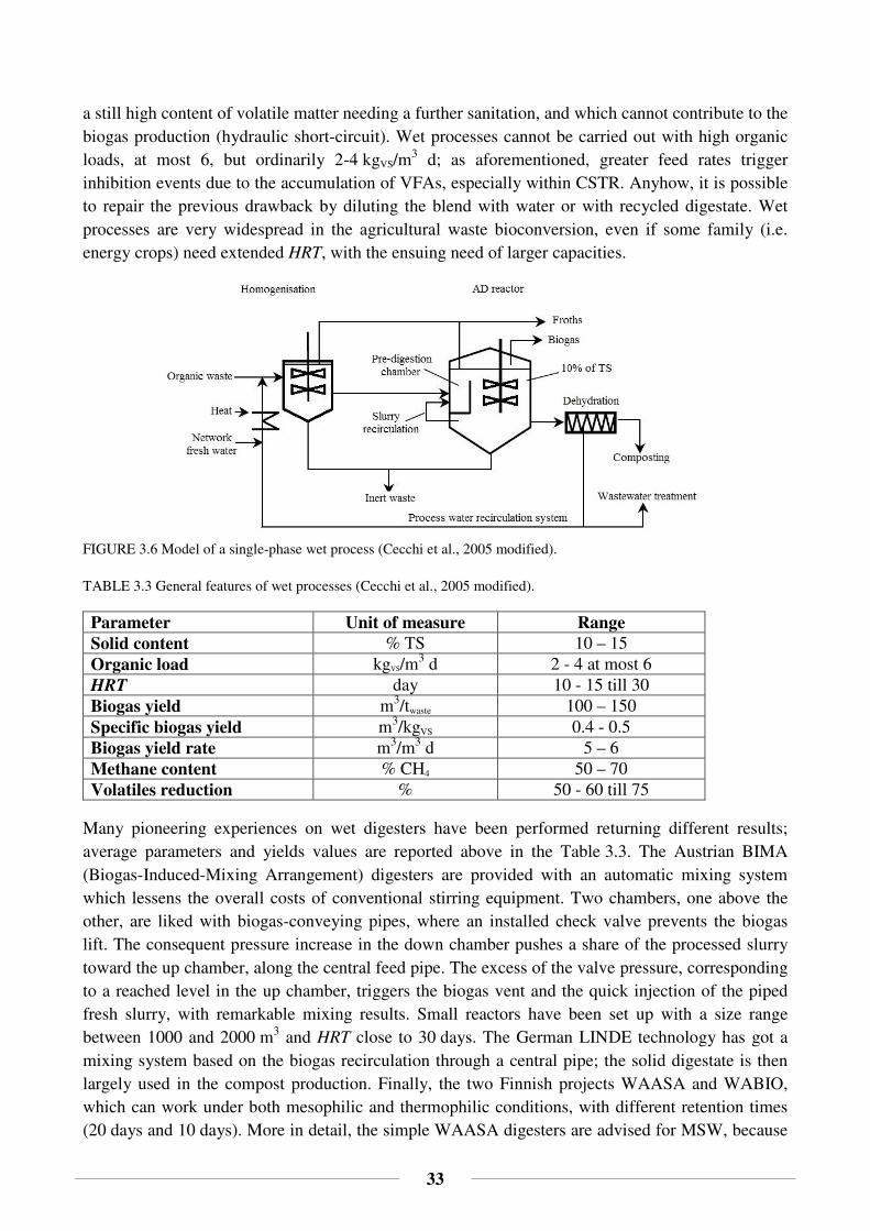
33

a still high content of volatile matter needing a further sanitation, and which cannot contribute to the biogas production (hydraulic short-circuit). Wet processes cannot be carried out with high organic loads, at most 6, but ordinarily 2-4 kgVS/m

3 d; as aforementioned, greater feed rates trigger inhibition events due to the accumulation of VFAs, especially within CSTR. Anyhow, it is possible to repair the previous drawback by diluting the blend with water or with recycled digestate. Wet processes are very widespread in the agricultural waste bioconversion, even if some family (i.e. energy crops) need extended HRT, with the ensuing need of larger capacities.

FIGURE 3.6 Model of a single-phase wet process (Cecchi et al., 2005 modified).

TABLE 3.3 General features of wet processes (Cecchi et al., 2005 modified).

Parameter Unit of measure Range Solid content % TS 10 – 15 Organic load kgVS/m3 d 2 - 4 at most 6 HRT day 10 - 15 till 30 Biogas yield m3/twaste 100 – 150 Specific biogas yield m3/kgVS 0.4 - 0.5 Biogas yield rate m3/m3 d 5 – 6 Methane content % CH4 50 – 70 Volatiles reduction % 50 - 60 till 75

Many pioneering experiences on wet digesters have been performed returning different results; average parameters and yields values are reported above in the Table 3.3. The Austrian BIMA (Biogas-Induced-Mixing Arrangement) digesters are provided with an automatic mixing system which lessens the overall costs of conventional stirring equipment. Two chambers, one above the other, are liked with biogas-conveying pipes, where an installed check valve prevents the biogas lift. The consequent pressure increase in the down chamber pushes a share of the processed slurry toward the up chamber, along the central feed pipe. The excess of the valve pressure, corresponding to a reached level in the up chamber, triggers the biogas vent and the quick injection of the piped fresh slurry, with remarkable mixing results. Small reactors have been set up with a size range between 1000 and 2000 m3 and HRT close to 30 days. The German LINDE technology has got a mixing system based on the biogas recirculation through a central pipe; the solid digestate is then largely used in the compost production. Finally, the two Finnish projects WAASA and WABIO, which can work under both mesophilic and thermophilic conditions, with different retention times (20 days and 10 days). More in detail, the simple WAASA digesters are advised for MSW, because

34

endowed with a vertical pulper, which makes the blend uniform and removes floating froths and sunken solids. The slurry is then set to a CSTR where the digestion successfully takes place, with yields in the interval 100-150 m3 biogas/Mg of slurry. Yet, the need of low solid content raises the water demand and thus the volume of the vessels, with remarkable costs.

3.4.2. Dry processes

Dry processes have developed since the Eighty’s and in the last years they are being preferred than wet ones. They are aimed at treating the organic substrate as it is, or better, avoiding plentiful dilutions and then limiting the wastewater amount. The solid content usually drops in the range 25-40%, therefore watering is needed for few samples with a lesser moisture (less than 50%), while air-drying for wet feeds. The biogas production may be very relevant if food waste is treated, but it undergoes a harsh decline when the amount of cellulosic waste (grass, trimmings) increases; that mostly occurs during the summertime, whence the seasonality of the yield. Earmarks of the process are summarised in Table 3.4. Microbial aspects are not perceptibly impaired by the water reduction, but on the other hand the mechanical components have to be utterly restyled: that implies a large initial investment for advanced equipment, but also ensuing construction (smaller volumes) and operative (heating, maintenance and stirring) savings. For instance, the matter has to be conveyed with belts, screws or pistons and pumped with expensive pumps for high-viscosity and high-concentrated fluids, therefore resistant to those external items that in wet processes could seriously damage the components (glass, sands, wood…). The short number of pre-treatment allows limited substrate losses: the only one is a screening able to remove particles greater than 40 mm. Chopping is often implemented, although sometimes limited to coarse sizes, with a fair energy saving. A way to limit the larger retention times (Li et al., 2011) is to speed up the start-up periods by implementing thermophilic conditions, with lightly higher costs in the heating system. CSTR configurations are quite expensive and thus seldom applied, because of the peculiar fluid properties; besides, plug-flow reactors are more widespread, in spite of mixing problems, but also the advantage of missing density separations. Generally, one may say that local events of extraordinary acidogenesis and ammonia accumulation are the main flaws of dry processes, whose recognised causes lead to an impairment of the methanogenesis.

TABLE 3.4 General features of dry processes (Cecchi et al., 2005 modified).

Parameter Unit of measure Range Solid content % TS 25 – 40 Organic load kgVS/m3 d 8 – 10 HRT day 25 – 30 Biogas yield m3/twaste 90 – 150 Specific biogas yield m3/kgVS 0.2 - 0.3 Biogas yield rate m3/m3 d 2 – 3 Methane content % CH4 50 – 60 Volatiles reduction % 50 – 70

The easiest geometry of dry reactors is depicted by two types of solid feed anaerobic digesters (SFADs), which are cylindrical vessels endowed with a recirculation system of the settled digestate and with stable performances (Abbasi et al., 2012). The difference between the two families is the seat where the liquid/solid separation occurs: in the SFAD-1 it is carried out within the digester,

35

whereas in the SFAD-2 in a separate unit. The digester produces little biogas on its own, and that is the reason why it is coupled with another reactor for the digestion of the produced leachate, with a high concentration of VFAs. That second reactor is often a UAF (up-flow anaerobic filter), later explained better, which is particularly suggested for liquid substrates with well-dissolved organic loads. This coupling allows a more fruitful biogas yield, up to 2 m3 per unit of reactor volume. The Belgian DRANCO technology (Figure 3.7) is considered the most performing anaerobic digester on the market, since low greenhouse gas emissions and operating costs along with high energy recovery and recovered material (Erkut et al., 2008). It consists in a vertical cylindrical chamber with the feed entry in the top and a conical-shaped bottom where an auger initiates the recirculation system usually having a somewhat relevant recirculation ratio α (6/7). Substrate types may be food waste, dewatered and pressed wastewater sludge, processed with a remarkably wide TS range (20-50%). The process is thermophilic (50–58°C), with roughly 20 days of retention and a productivity of 100-200 Nm3/Mg of substrate (Arsova et al., 2010). On the contrary, the Swiss KOMPOGAS (Figure 3.7) involves a horizontal reactor with internal slow-rotation axial paddle mixers aimed at the mass homogenisation, the gas rescue and the coarsest inert fraction flotation. The optimal solid content range is quite narrow (23-28%), since on one hand greater TS make the matter movement more energy-demanding, on the other hand lower TS reduce the flotation performances. The recirculation piping mostly conveys process wastewater, in order to keep the suitable solid content. This reactor was chiefly designed for OFMSW thermophilic digestion and for an integrated production of solid (fresh) compost and a liquid fraction that, once further processed, might avail as soil amendment. The whole cycle lasts more or less one month, where three days for the substrate preparation, twenty of HRT and ten for the aerobic composting. Sometimes, the smallness of the reactors involves the implementation of parallel configurations for large scale applications. The last configuration is the French VALORGA (Figure 3.7), very peculiar, since the mixing necessities are made up with the recirculation of the only biogas from the bottom of the vessel, with vents each 15 min roughly. It is clear that the goal is fulfilled by using normal compressors instead of the aforesaid advanced hydraulic pumps. It can be considered as the sample of the biogas-sparging reactors, usually characterised by large sizes. Nevertheless, the system is extremely sensitive to coarse matter settlement, whence the need of regular cleanings for obstructions prevention and of wastewater recirculation (like KOMPOGAS) for the preservation of TS near to 30%. Even this system was planned for OFMSW and for the organic fraction from not separated collection (needing pre-treatment), but under mesophilic conditions mostly. Retention times range between 18 and 25 days, with a productivity of 80-160 Nm3/Mg of feed.

FIGURE 3.7 The three most common configurations of dry reactors. Rightwards: DRANCO, COMPOGAS and VALORGA (modified from Cecchi et al., 2005).

36

3.4.3. Semi-dry processes

Semi-dry processes are a half way between the previously shown wet and dry ones, thought and adjusted by Italian boards. They handle pre-treated feedstock with a solid content of 15-20% which CSTR reactors can fit, under both mesophilic and thermophilic conditions. It is quite difficult to characterise semi-dry reactors individually, because the majority of their earmarks are proper of the two original processes. The vessel bottom cleaning is a compulsory cost, due both to faint density separation phenomena and to the efficiency of the outlets for biogas recirculation. The contained solid content allows money savings on the use of normal stirrers and hydraulic pumps, but on the other hand significant costs of pre-treatment and large vessels realisation have to be often faced. Anyhow, the energetic operative outgoings are often amply offset by the produced bio-methane combustion. It is not yet easy to try to enumerate the potentialities of the system, since the shortage of applications; average work intervals of the Italian experimental SNAM reactor are described in the Table 3.5. Surely, a proven evidence (Cecchi et al., 2005) are the higher performances in terms of SGP (0.4 vs 0.2 m3/kgVS d) and removed VS (50 vs 20%) of thermophilic treatment than mesophilic one, with the same HRT and OLR.

TABLE 3.5 General features of dry processes (Cecchi et al., 2005 modified).

Parameter Unit of measure Range Solid content % TS 15 - 20 till 25 Organic load kgVS/m3 d 8 - 12 till 18 (thermophilic cond.) HRT day 10 - 15 Biogas yield m3/twaste 100 - 150 Specific biogas yield m3/kgVS 0.3 - 0.5 Biogas yield rate m3/m3 d 3 - 6 Methane content % CH4 55 - 60 Volatiles reduction % 40 - 50 till 60

3.5. BIOMASS PRESERVATION SYSTEMS IN TWO-STAGE PROCESSES

The potentialities of two-stage systems have not yet been exhaustively found out and valorised, as higher bio-methane yields due to an optimal serial process subdivision, a more correct management of the microbial growth needs (e.g. pH) and of the residence times, cannot offset the costs of larger initial investments and management (more vessels) than the more technologically advanced single-stage processes (Weiland, 2005). In this configuration, only the methanogenesis is separate from the others, but it is even possible to have both vessels devoted to the four stages of the digestion: a high-loaded main digester ensued by a low-loaded secondary one. This last scheme is particularly recommended for energy crops and high concentrated sludge. The first group of digesters, devoted to the hydrolysis, acidogenesis and acetogenesis, is designed according to a type of first-order kinetics; unfortunately, the hydrolysis is often adversely affected by high cellulose concentrations. A short quantity of methane is yielded during that procedure as well. Then, the second group hosts the methanogens activities, where again the slow growth speed of the last ones sets the structural design rules. In some configurations, the acetogenesis belongs to the second group, but that choice does not involve essential changes in the structural design, since that is not a limiting stage. Usually, the reactors plan is constrained neither by the geometry nor by water content, and even the design mathematical models are the same ones, despite the outcomes may be dramatically different,

37

like low HRT and sizes in two-stage scheme. Notwithstanding, the configuration of the two vessels is the same, since it is often set by the choice of the water content. Inversely, a parameter having remarkable effects on the process is the presence of a biomass preservation system, whose peculiarities are explained in the follow-up. As aforesaid, reactors with biomass preservation may be provided with either recirculation piping or inner immobilisation frames. This type of equipment is especially needed in the second vessels, for the methanogenesis fostering. As far as biomass immobilisation strategy is concerned, a thorough removal of suspended particles is carried out on the effluents of the first reactor, with the drawback of nutrients loss and TSV removal lessening. Nevertheless, the technique allows the development of advanced resistance skills of the biomass, both over inhibiting substances (ammonia) and on bearable OLR (up to 8 kgVS/m

3d). The geometries later presented were developed by different German companies. Firstly, BTA reactors work under wet (10% of TS) and mesophilic conditions and may be easily implemented in single-stage processes. It involves ordinary pre-treatment plus a substrate preparation stage inside a hydro-pulper and an additional pasteurisation, where two streams are later generated. The liquid is sent to the anaerobic digester, whereas the solid to the hydrolysis vessel: in turn, here it produces a liquid flow that is merged with the previous one, and a solid flow which may be recirculated and later composted with other solid effluents. BTA technology is quite complicated, since it involves setup and management of four reactors, but satisfactory yields as well (Table 3.6). Retention time is between 12 and 17 days and average biogas production from 85 to 95 Nm3/Mg of feed.

TABLE 3.6 Standard operative conditions and yields of the BTA process (Bozano Gandolfi and Wiljan, 1999 modified).

Parameter Unit of measure

Single-phase Double-phase Hydrolysis Methanogenesis

Reactor temperature °C 37 37 HRT day 14-16 2-4 3 Biogas yield Nm3/twaste 80-90 110-120

0.5-0.55 Specific biogas yield m3/kgVS 0.38-0.42 Methane content % CH4 60-65 30-50 65-75 Heat yield kWh/t 305 415

225 Energy yield kWh/t 165

In the Biopercolat, hydrolysis and acidogenesis are undertaken under dry micro-aerophilic conditions and within a plug-flow vessel; that reduces the retention times (globally 7 days), but the biogas yield as well. The process is further speeded up thanks to the recirculation of the leachate, collected from the mesh-like (1 mm) bottom of the reactor. Finally, STRABAG is a long chamber with a rectangular cross section and stirrers along the main dimension. It is considered as a plug-flow reactor, as the feed (15-45% of TS) is carried throughout it thanks to an apt conveying system. It can work under either thermophilic or mesophilic conditions bringing about biogas yields close to 100 m3/Mg of feed (Ostrem and Themelis, 2004).

Reactors without microbial biomass preservation work very well with many types of organic waste, but cellulose, and with high OLR (close to 7 kgVS/m

3/d). Maybe, the most important aspect is the “buffer effect” played by the upstream reactors, because less sensitive to strong substrate increases and pH lowering. An example of this system is the German BRV, working with plug-flow reactors and under dry conditions. The hydrolysis is exceptionally carried out under micro-aerobic

38

conditions, which allows quicker results despite the loss of the substrate share needed for aerobic biomass growth. The Schwarting-Uhde, of the same Country, works under thermophilic conditions, with wet sludge that is impulsively pumped from the bottom of two digesters; a corresponding quantity of biogas vents from the vessel top, together with liquid effluent. The substrate is carefully cleaned, crushed and then diluted, so that to limit obstruction problems of the bottom openings during the pumping. Great performances of this technology are proven by short retention times (11-18 days), high SGP (0.83-0.88 m3/kgVS) and TVS removal (80-85%).

3.6. RATE OF FEEDING

As formerly hinted, the “work rhythms” of the anaerobic digester are key structural design factors; the parameters which they depend on are the HRT and the SRT. The goal of this section is to go thoroughly in the structural and technical properties of some reactors geometries previously explained, as well as to introduce some of the most common configurations applied at a small scale in developing Countries (like China and India). There, they avail many countryside realities and offer a cheap and green fuel, mainly used for cooking. The technical simplicity and economic feasibility allowed a rapid and worldwide diffusion of these plants, even inside unexpected places like the Indian Nisarga-Runa biogas plant, within the jail courtyard. Conversely, large scale plants are mostly widespread in developed Countries, where sometimes the biogas production is not the main target, but the cheap and efficient stabilisation of bulky organic loads; therefore, some plants have a negative energy balance.

3.6.1. Low-rate digesters

Low-rate fermenters are characterised by the equivalence between HRT and SRT, which may be close to 40-50 days. Even anaerobic-activated sludge vessels, planned for being part of high-rate processes, are nowadays still considered as low-rate one (HRT = 10-15 days). Feedstock is chiefly represented by dilute animal dung, thus very elementary and not much fruitful. According to Evans et al. (2015), the 70-80% of the operative costs is ascribed to the fermenter, while the residue to the maintenance. Regardless of the advantages, the system suffers from intuitive and already explained reasons, like the lack of an agitator, the enduring loss of active biomass with the clarified effluents and the establishment of average growth conditions which should satisfy every microbial community. At a small scale, it is possible to have three configurations of plants: fixed-dome, floating-drum and balloon (Sasse, 1984). Fixed-dome plants (Figure 3.8A) are underground containers (at most 20 m3 bulky) receiving quite liquid substrates (4-8% TS) from a superficial sink. The material inside the vessel undergoes a slow anaerobic digestion (HRT = 50-66 days), and the stripped biogas occupies the upper volume (gas holder), where a sealed and weighted entry hatch prevents its escape (whence “fixed”). Therefore, the biogas pressure increases and it pushes against the water (scum) level, in turn moving the slurry along a pipe and out of the reactor, into a superficial overflow tank. The overflowing pipe inlet is placed near the surface, so that to convey the digested slurry only, which, being lighter than the fresh one, floats and then it is pushed downward. Since the absence of moving devices and rusting steel, the life of the plant may be quite long (20 years) and with low maintenance costs. If the underground location is weatherproof and not much impacting on one hand, on the other hand does not permit high digestion temperatures. Despite the construction easiness and cheapness, trained

39

experts presence is strongly recommended, even because the stern safety problems deriving from high biogas pressures, which could crack the vessel walls as well. Floating-drum plants (Figure 3.8B) are similar to the previous ones, but the gas holder is not joined with the reactor, hence it is free to float according to the biogas quantity, either on the slurry or on a water jacket. In addition, it is supported with a guide frame able to prevent it from going out the planned track. The biogas pressure can be easily inferred from the gas holder lifting; it usually does not bring safety issues about, hence no safety seal is present. In addition, where the diameter is greater than 1.5 m, a central vertical wall is set up, in order to improve the process conversion and thus avoid hydraulic short-circuits. Typical operative parameters are the HRT in the interval 40-55 days, the solid content close to 9% and the fermenter volume from 1-8 up to 100 m3. This system is surely easier, safer and more extensively applicable than the former one, although there are great maintenance costs and issues of short life (at most 15 years) and corrosion. This last aspect can be lightly confined with the replacement of steel with nonrusting plastic materials, like HDPE, but not PVC, because not lightproof. Nevertheless, the pressure constancy of the gas allows its direct combustion within engines, opposed to the fixed-dome plants; actually, that is only a potentiality, because engines need huge quantities of biogas and therefore very large gas holders. The last and quite curious configuration is the balloon plant, a large rubber or plastic bag provided with a feed and a discharge pipe like the previous ones. It works more or less like the fixed-dome vessel, since the biogas accumulates in the top and then it vents out under controlled conditions. The “limpness” of the material, often inelastic and resistant to UV beams (Red Mud Plastic, Trevira or butyl, not PVC), makes the vessel more liable to agitations, therefore favouring the process. In larger scale plants, the inflatable balloon only covers the vessel; anyhow, the useful volume for the biogas accumulation is somewhat limited. Advantages concern the broad variety of treatable substrates (water hyacinths too), the overall low costs (hauling and installation), the high operative temperatures and the easy maintenance and cleaning. Conversely, the system is very prone to impairments which cannot be aptly refurbished, as well as to low temperatures and sharp variations of it, and hence to a short lifetime (5 years).

FIGURE 3.8 A: Fixed-dome and B: Floating-drum plants (Evans et al., 2015).

Among the large scale configurations, covered lagoon digesters are the most elementary ones (Figure 3.9A). It is a system of two serial ponds, where the upstream and covered one is devoted to the anaerobic digestion accomplishment, while the downstream and smaller one to the collection of the liquid effluents; usually, the solid content does not exceed the 2%. The produced biogas swells the impermeable wrap like in the balloon digesters. The production trend is extremely changeable, hinging on the environmental temperature: that is the reason why large volumes are needed for high HRT when the biogas production grazes minimal values (cold weather). On the other hand, the lack

40

of temperature and process controls is a technical and economical saving. Plug-flow and ASBR reactors are often ranked in the low-rate and large scale plants but, as they have already been explained in the previous paragraphs, only some additional operative hints are quoted here. Surely, they are more advanced than lagoon ones, since the vessels are made of concrete and provided with a careful temperature control, so much so that one may decide the working conditions. In plug-flow fermenters, thermophilia is the most fruitful one, processing slurries with a solid content of 11-14% and with a HRT of 15-20 days. Instead, ASBR fermenters are often employed in the digestion of highly dilute manure (1% TS), even if they could work in broader solid ranges. Fixed-film fermenters (Figure 3.9B) rely on a peculiar biomass immobilisation technique, that is, a motionless bed of packed media, such as wood chips, which is continuously crossed upward by the substrate. In turn, its solid content has to be quite small, since obstruction problems could arise. That is the reason why a solid/liquid separation unit is needed upstream the treatment, so that to reach a short solid content (at most 5%): this operation potentially reduces the total biogas yield. The system is even provided with a recirculation circuit which grants a HRT close to 5 days. Opposed to fixed-film reactors, suspended media ones are based on the mobility of the support where the biomass was anchored. It is represented by the particles of the digested matrices which settle and are stirred by the fresh influent arrival. Since this family of reactors are implemented in high-rate processes as well, they will be better explained later.

FIGURE 3.9 A: Covered lagoon and B: Fixed-film plants (Evans et al., 2015).

3.6.2. High-rate digesters

The passage toward high-rate fermenters was reachable in many fashions, such as: the rise of the SRT through the implementation of attached or suspended biomass growth equipment; the drastic reduction of the HRT and the vessel capacities; the increase of the organic matrix within the influents (digester loading). The aforementioned CSTR and its version with biomass immobilisation, called anaerobic contact reactor (ACR), belong to the so named first generation high-rate fermenters. CSTRs, mainly used for animal waste treatment, were the first endeavour toward high-rate digestion modes, but the HRT remains still high (15-20 days). Thanks to the stirrer, the volumes can be remarkable, up to 500 m3. ACRs improved the performances of the previous ones thanks to the setup of a settling tank downstream, where the active biomass, settled by gravity, was recycled and mixed with the fresh influents carefully. Performances can be negatively affected by an incorrect sedimentation, as well as by large volumes, where the blending is likely to lose its benefits. ACRs are chiefly used for dairy and sugar beet waste.

41

The variety of geometries ranked as second generation high-rate fermenters is characterised by the increase of the SRT without any recirculation tool, thus only with biomass immobilisation systems. Up-flow anaerobic filter (UAF) is a cylindrical vessel crossed by an upward stream of feed and where it is possible to distinguish three sections (Figure 3.10). Firstly, a chamber in the bottom, where the entered feed meets a horizontal barrier with regularly placed dispersion rings through which it gets distributed in the upper volume. This second capacity is randomly filled with inert support fragments (stone, plastic, ceramic or fired clay), which the biomass can attach upon and degrade the organic load. It is evident that the more soluble and dilute the suspended substrate, the more successful the result, so much so that coarse and plentiful solid particles bring about clogging issues. The last part is a domed sector aimed at the collection of the treated effluent and biogas. The stern and inflexible controls over the influent induced the adjustment of another configuration named Down-flow stationary fixed film (DFSFF), able to process up to fairly concentrated sludge. Here, the fresh influent, often merged with recycled effluent, is sprinkled in the headspace onto a support of inert particles like the previous one, where it moves downward, up to be collected in the bottom. The dispersion of the feed is enhanced by the biogas stripping as well. Fluidised and expanded bed reactors (FB/EB) display a tripartite structure similarly to the UAF (Figure 3.10), but they are based on the suspended biomass growth strategy, carried out with a bed of fine and inert media (e.g. sand or alumina). These systems are suitable for soluble and easily degradable substrates like whey and black liquor condensate, but even raw sewages. The difference between the two reactors is the bulkiness of the bed expansion, related to the influent rate: 10-15% of expansion is considered expanded, whereas 15-25% fluidised. The most popular high-rate digester geometry in the word, very used in wastewater treatment plants since the high performances with high COD, is the up-flow anaerobic sludge blanket (UASB). It shares with the UAF many structural and operative earmarks (Figure 3.10), but here the arising problems of obstruction are worked out by replacing the solid support with a self-sufficient “biomass support”. In other words, UASB relies on the formation of heavy and bacterial lumps (blanket) which are only lightly suspended when they are crossed by an upward influent. The biogas is gathered inside superficial gas/liquid/solid separators, which let the collection of the liquid phase as well. The ability of microbes to group in more or less heavy lumps hinges on the type of substrate: in particular, the keenest ones are sugar and highly volatile acid waste. It is the chief hindrance to the performances of UASB reactors, which is partially overcome with the addition of active biomass from other UASB.

FIGURE 3.10 The most common second generation high-rate fermenters. Rightward: up-flow anaerobic filter (UAF), fluidised and expanded bed reactors (FB/EB), up-flow anaerobic sludge blanket (UASB) (Evans et al., 2015).

42

The so named third generation high-rate fermenters is a still developing family aimed at enhancing the earmarks of the former group (e.g. biomass immobilisation) and at striving to broaden the variety of substrate which can be processed. The most successful achieved outcomes are hybrid and modified geometries. UASB-UAF hybrids, like the up-flow sludge-bed filters (UBF), fulfil degradation performances otherwise inaccessible by the two systems separately. The reaction column is split up in two parts: the upper and thinner (1/3) one acts as both biomass preservation and solid/liquid/gas separation unit (UAF), while the lower one is the sludge blanket where the contact between biomass and substrate is optimised. Finally, valid modified UASB technologies have been adjusted for treating different waste, such as multi-plate anaerobic reactor (MPAR) and the Biopaq UASB reactor.

3.7. FEEDSTOCK PRE-TREATMENT

Substrate pre-treatment is an upstream procedure aimed at the removal of those fractions which could hamper the digestion stages. The choice of pre-treatment stages should consider not only the type of organic matrix and the planned digestion process, but even the fate of the effluents. For example, the solid digestate may be valorised within suitable incinerators or treated for the achievement of high-purity fuels; that is the reason why high quality controls are required before the digestion. Once received within the plant, the substrate is deprived of the metals, which could scrape the facility and which generate a “free of charge” flow of raw materials. Ferrous metals are collected with magnetic separators, while non-ferrous ones with eddy currents separators (Cecchi et al., 2005). The second stage is the removal of non-biodegradable plastics and inert materials (sands, gravels…) which could provoke obstruction and abrasion issues. The goal is achieved with serial treatment including sieves, ballistic and density separators: wet processes with decanters and floaters are carried out only if the digestion is planned under wet conditions. Then, a suitable particles size for a correct digestion (d < 50 mm) is reached with crushing operations: as a matter of fact, the smaller the size, the greater the free surface of the substrate which can be break down by microorganisms. Unfortunately, although the biogas production rate rises, the methane content is not sensitively affected. Moreover, it is important to mention some pre-treatment related to particular realities. When OFMSW is the chief feedstock, the bags laceration is the first stage, which should be actually quite “slight”, in order to avoid mixing the organic fraction with the undesired one that has to be later removed. Novel physical (thermal, mechanical), chemical (oxidation) and biological (enzymatic) pre-treatment was proposed for improving the hydrolysis of tough and stable matrices (i.e. grass, wood). In particular, the very strong and fast thermal pressure hydrolysis (T = 230°C and p = 20-30 atm) increases the biogas production and it may lower the overall substrate retention time. On the contrary, the effectiveness of enzymatic pre-treatment is rather controversial. On one hand, it lessens the substrate viscosity and it prevents the formation of a floating film, with the ensuing quicker degradation of polysaccharides the biogas yield rise till 20% roughly. Conversely, not only the final methane content does not undergo noteworthy improvements, but actually the enzyme may become a good substrate for anaerobic microbes, attacking it with their own proteases. Even the killing of pathogenic bacteria and viruses, hazardous for workers’ safety, might be considered as a type of pre-treatment, since it is carried out before the digestive procedures. It consists in a one-hour pasteurisation at T = 70°C (Evans et al., 2015) and a sterilisation at T = 130°C of the substrate, where the difference is not only the higher temperature,

43

but the higher treatment duration as well; it is quite obvious that the slightness of the first one involves less properties losses. In conclusion, what is important to highlight is that any pre-treatment is unavoidably related to more or less sharp volatile solids losses (up to 15-25%): their containment is the challenge for the new technologies. Once pre-treated, the substrate has to be prepared for the AD. The planned solid content may be reached with the dilution with different streams like sludge, leachate, wastewater or even network water. The homogenisation devices depend on the substrate moisture: hydro-pulpers for semi-dry and wet processes and cochlea mixers for semi-dry and dry ones. The last step is the temperature control, achievable with two fashions. External controls involve the use of heat exchangers inside the vessels or the heating of the diluting streams. Internal controls may be based again on heat exchangers, but even on the injection of hot steams; the prevention of bacterial thermic inhibition is possible thanks to a robust simultaneous stirring.

3.8. BIOGAS PURIFICATION

Biogas is not the only interesting product of the AD, but surely the most beneficial. It is usually described with two quantities, the flow and the methane content, which could have notable variations with respect to the average values (60-140% and 45-65%). Besides, they have got an opposite behaviour: the greater the flow, the lower the CH4 content (beginning of the process) and conversely (end of the process). As said before, there may be a significant share of organic matter in the effluents, because of both the non-biodegradability of the substrate and the incompleteness of the process; obviously, one is interested in minimising it, since it is not converted into biogas. The recovery is another important stage which needs an upstream study, because of the presence of three substances with different solubility. As a matter of fact, CO2 partially combines with water, giving rise to carbonic acid which contributes, together with ammonium, to the buffer effect of the system. Despite insoluble, H2 usually does not leave the water phase, because of its rapid consumption by hydrogenotrophs (Cecchi et al., 2005). On the contrary, methane suddenly moves from the water to the gaseous phase above; that phenomenon, known as stripping, may be generally explained with the following relationship for the transfer velocity v:

4 = !t!# = (uv wt − xj

py (3.14)

Where C is the concentration of dissolved gas in the liquid phase (M V-1 T-1), KL is the global coefficient of mass transfer (V A-1 T-1), a is the specific surface of the gas bubble (A V-1), pg is the gas partial pressure, and H is the Henry’s constant (p V M-1). More detailed analysis for air bubble displayed that the stripping time is directly proportional to v and inversely to the diameter. Besides, in more soluble gasses the stripping time often implies a partial entrance to the liquid phase.

In spite of the various handlings the biogas may have, it cannot be used as it is, since dirty. Adjustment treatment (cleaning and upgrading) depends on the earmarks and on the planned uses of the biogas, but one may generally argue that it is aimed at the preservation of the transport and burning devices and the compliance with the emissions policies. Table 3.7 briefly enumerates the chief impurities, their drawbacks and likely ranges of concentration, depending on the type of digested substrates. Just out of the digester, the biogas is filtered, with the removal of the conveyed drops and dusts (d < 10 µm) which could impair pipes and devices.

44

TABLE 3.7 Biogas impurities (Ryckebosch et al., 2011; Naja et al., 2011).

Substance Concentration Possible impacts Dust traces Settlement and obstructions of equipment Water 10-15% Reaction with H2S, NH3 and CO2 with the

formation of corrosive compounds Accumulation in pipes

Hydrogen sulphide 0.005-2% Corrosion of equipment Toxicity (> 5 cm3/m3) Combustion with O2 and formation of dangerous SO2 and SO3 forerunners of acid rains

Carbon dioxide 15-60% Lessening of the heating value Siloxanes 0-0.02% Combustion with O2 and formation of abrasive

SiO2 crystals Hydrocarbons (benzene) 0.17-2.1 mg/m3 Corrosion in engines due to combustion Ammonia < 1% Corrosive when dissolved in water O2 and air 0-3% Rise of the explosiveness of the biogas Chlorine 5-40 mg/m3 Corrosion in combustion engines Fluorine 20-23 mg/m3 Corrosion in combustion engines

3.8.1. Dehumidification

The first type of treatment is the dehumidification, not only because water lessens the heating value of biogas, but even because the water condensation might give rise to system failures. Generally, the amount of water vapour saturating the biogas is proportional to the temperature and advanced applications of biogas need strict controls over it. For instance, water in pipeline gas must be lower

than 10 mg/m3 and the ∆T between the 99% of the winter design temperature of an area and the dew point of compressed natural gas (CNG) for vehicle fuel must be at least 10 K (Rutledge, 2005). Condensation within refrigerators and collection of the water is maybe the most intuitive fashion of moisture abatement: the condensate often holds other soluble hazardous substances. There are different devices used for that purpose, but the greatest limit is the impossibility to reach dew-points lower than 0.5°C, owing to the formation of ice on the surfaces of the heat exchanger. Lower values can be reached with a preliminary compression: the higher the pressure, the lower the dew-point. Some of the most widespread configurations with the related water separation fashion: demisters (wired mesh with a d = 0.5-2 nm), cyclone separators (centrifugal forces), moisture traps (gas expansion) and water taps in the biogas pipe. An advanced dehumidification (dew-point up to -20°C at patm) can be performed with chemical methods which usually need high-pressure conditions. Adsorption, that is the superficial retention of gaseous molecules due to an electrochemical interaction with a surface, employs silica, activated carbon, aluminium or magnesium oxide. Two columns are used, one for the adsorption and the other for the regeneration of the materials at low pressures (desorption) and the collection of the water. On the contrary, the absorption, that is the physicochemical uptake of any kind of molecule within a medium, uses liquefying chemicals like tri-ethylene glycol (regenerated at a T = 200°C) or hygroscopic salts (not regenerated).

45

3.8.2. Desulphurisation

Even if present in imperceptible quantities (100-3000 ppm), hydrogen sulphide is a strong and poisonous corrosive; it is evident that frameworks upstream the desulphurisation stage have to bear its effects. Its control is important not only for the preservation of the equipment, but for the compliance with the emissions limits as well, since its combustion gives rise to sulphurous acid, a forerunner of acid rains. It may be removed together with the water, but high concentrations need suitable procedures, wet or dry and during or after the digestion, until the concentration drops below 250 ppm. An easy external wet configuration is the combined absorption with water of H2S and CO2, which are more soluble than CH4. Pressurised biogas (1-2 MPa) is injected in the bottom of a suitable vertical chamber (scrubber), where it meets a water flow in counter current. The increased solubility of CH4 due to higher pressures suggests the setup of a depressurising flash tank for the wastewaters, whence the rescued methane is recycled with the incoming biogas. High yields (95%) are accompanied by huge quantities of water needed for an acceptable decline of the H2S, with the ensuing high costs of pumping, storing and regeneration of the wastewaters. It can be partially worked out with the cheap use of sewage wastewaters, but more “correct” techniques lessen the amount of water by employing absorbing chemicals and the regeneration of the wastewaters, although not always done. The use of strong bases (e.g. NaOH) brings about insoluble salts (Na2S and NaHS) and may imply a later adjustment so that to avoid pH far away from the basicity. This method proves particularly efficient when a fair amount of H2S meets a valid quantity of solvent/reagent: therefore, careful controls are always needed. Similarly, the chemical scrubbing with organic solvents, like polyethylene glycol, can absorb the two gasses and water too better than water, whence smaller volume of solvent to be circulated and renewed. Less widespread processes involve the forced solution of H2S inside high-pressure water with CO2, later released with the pressure drop (stripping). It is clear that wet processes have to be carried out before the dehumidification. On the contrary, dry processes involve the use of a re-generable adsorbing substance able to react selectively with H2S in the main stream. Therefore, it is important have some thermodynamic and physic knowledge about the H2S, like pressure, temperature, concentration, biogas flow speed and contact times, as well as the adsorbent cycle. Iron III oxide (Fe2O3) and hydroxide (Fe(OH)3), kept inside wood pellets so that to broad the active surface, give rise to iron sulphides and they can be easily regenerated in a separate chamber with air (or, more seldom, water), followed by a filtration of the solid sulphur lumps (formulas 3.15-3.17). The exothermicity of the regenerating reaction might raise issues of pellet self-ignition if air flow and temperature are not controlled.

Fe�O� + 3H�S → Fe�S� + 3H�O (3.15)

2Fe(OH)� + 3H�S → Fe�S� + 6H�O (3.16)

2Fe�S� + 3O� → 2Fe�O� + 6S (3.17)

A similar type of treatment during the biogas production involves iron chlorides (FeCl2 or FeCl3), giving rise to the precipitating iron sulphide (formulas 3.18 and 3.19):

2Fe�_ + 3S�8 → 2FeS ↓ +2S (3.18)

46

Fe�_ + S�8 → FeS ↓ (3.19)

Adsorption with active carbons need more frequent, expensive and solvent-based regeneration techniques, which can be afforded only when the H2S content is very limited; anyhow, in many cases the exhaust active carbon bed is not regenerated. This treatment is optimised under particular thermodynamic conditions (p = 700-800 kPa and T = 50-70°C), easily achievable with a compression, and the reaction rate can be enhanced with the addition of KI and H2SO4. A novel dry technology, quite cheap in terms of management costs, is the biological desulphurisation, performed either outside or inside the fermenter. It consists in a panel of mesophilic (35°C) and autotrophic sulphur-containing compounds degrading microbes (like Sulfobacter oxydans and Thiobacillus) able to oxidise H2S to elemental sulphur and sulphurous acid, according to the reaction:

2H�S + O� → 2S + 2H�O (3.20)

It is clear that a small amount of air has to be granted (2-6% of O2), being careful that a higher concentration of oxygen (6-12%) brings about an explosive blend with biogas. The external process involves a bio-filter filled with plastic frames where microbes dwell: it is arranged within a column where it is crossed upward by a stream of biogas and air. The filter is sometimes cleaned up so that to prevent the metabolites accumulation, as well as continuously crossed with a recirculated liquid solution of nutrients needed by the organisms. Moreover, even ammonia can be at once removed. In internal treatment, the panel is directly arranged upon woody or fabric frames within the digester, usually in the headspace; the efficiency is in the range 80-99%.

3.8.3. Trace elements removal

Further purifications concern peculiar rare elements being usually more widespread in landfill gas than in AD biogas. Halogenated carbons hydrates are mostly chlorine/fluorine-containing organic compounds which are corrosive for gas engines. The most efficient removal technique employs pressurised tube exchangers, where they, being larger than CH4, CO2, N2 and O2, are trapped in the frame of activated carbons, later regenerated at 473 K. Air is surely liable to be inhaled with landfill gas, since often collected with vacuum permeable pipes: as hinted in the desulphurisation, O2 concentrations till 4% are not hazardous, oppositely in the range 6-12%. Besides, N2 raises the concentration of inert substances within biogas. Preventing their entrance with meticulous controls is better than treating the contaminated gas. Siloxanes are linear or cyclic silicon-containing organic molecules, often with radical groups (e.g. methyl, ethyl). The main problem they cause is the settlement of small abrasive quartz crystals after their combustion, even though the bearable siloxanes limit in biogas is widely changeable and dependent of the claims of the manufacturers (0.03-28 mg/m3). The removal of siloxanes is not an easy operation, since their loathness in being chemically and biologically degraded (Ryckebosch et al., 2011). The less advisable techniques are chemical treatment with strong bases, since it brings about many settling carbonates, and physical absorption with long carbon-chain organic solvents (i.e. hydrocarbons), which is compromised by the high volatility of the solute. On the other hand, more efficient removals were proved with strong acids and chemical absorption. The cryogenic separation, based on the liquefaction at different temperature and pressure ranges of the substances, showed good results at low temperatures (203 K). Finally, adsorption techniques proved more

47

efficient with silica gel than with activated charcoal, although sternly damaged by the presence of water, whence the need of carry a previous dehumidification out; in both cases, the desorption is performed at 523 K.

3.8.4. Carbon dioxide removal

Treatment processes may finish with the CO2 abatement, aimed at increasing the CH4 concentration and the heating value, getting the so called enriched biogas. As CO2 can be efficiently removed along with other chemicals with one of the aforesaid procedures, in the follow-up only additional techniques are proposed. A type of chemical scrubbing that was inaccessible to the H2S removal employs di-glycol or alcanol (mono/di-ethanol) amines, which are poisoned by H2S traces: their regeneration involves steam or heat. The adsorption and desorption reactions, involving the same chemicals, are reported beneath and may have 99.5% of efficiency:

R NH� H�O CO� ↔ R NH�_ HCO�8 (3.21)

Pressure and vacuum swing adsorption (PSA and VSA) are operations whereby compressed molecules of CO2 (p = 800 kPa) temporarily stick upon the hollows of a catalytic adsorbing sieve (e.g. zeolite, activated carbon, alumina and silica gel) which is later re-generated by declining the pressure. H2S is forbidden to be removed with these processes, since the poisoning to the catalysts; conversely, O2 and N2 can be removed by changing the pressure and the size of the sieve. As formerly hinted in the dehumidification, each PSA configuration is provided with more chambers (adsorbers), each of which hosts one operation at a time (Figure 3.11): adsorption, where CO2 is trapped along with a fraction of CH4; depressurisation, where a small drop of pressure allows the rescue of the trapped CH4; desorption, where a more advanced pressure decline regenerates the catalysts; pressurisation. Relevant energy savings can be achieved by coupling compression and release stages. In the VSA scheme, the depressurisation stage is replaced by the use of a vacuum, discharging CO2 into the atmosphere; this is the main weakness of it, since small quantities of CH4 could be already present, and everyone is aware of the higher GWP of CH4 than CO2.

FIGURE 3.11 Scheme of a PSA system (Persson, 2003).

48

The cryogenic separation is a somewhat insightful way to purify biogas, even if, since the high costs for reaching low temperatures, it is chiefly recommended when one wants to get liquid bio-methane (LBM), equivalent to the liquid natural gas (LNG): otherwise, once purified, it has to be warmed up again. The process consists in a gradual compression and cooling of the carefully dried biogas up to p = 8 MPa and T = 218 K. Then, it is expanded inside a chamber till 0.8-1.0 MPa, with the ensuing cooling down to 163 K: here, the methane-rich (97%) gaseous phase and the solid CO2 are stable, thus the separation may be successful. The layer of liquid CO2 formed at the intermediate stage (228 K) dissolves further impurities and traces of CH4, which are later recovered. The last family of CO2 removal methods are embodied by elongated chambers hosting a separation membrane, whose working principle is the selective permeability of the membrane towards gaseous molecules. Whatever the type is, high efficiencies cannot be reached directly, therefore it is expedient both arranging a series of membranes and recycling the still CH4-rich gaseous discharge. High-pressure (or gas-gas) separation membranes, made of acetate-cellulose, work with compressed gas (p = 2.0-3.6 MPa) crossing them. Small polar molecules of water, CO2 and residual H2S go out the system from a side outlet, while CH4 and N2 carry on their transit and reach the opposite side of the membrane. Despite the quite high second-stage yield (96%), a fraction of methane is relentlessly lost in the waste gas (10-25% of it), getting environmentally harmful the direct discharge into the atmosphere: possible solutions are the flaring or, more cleverly, the heat recovery in a steam boiler (Ryckebosch et al., 2011). Conversely, the more recent low-pressure (or gas-liquid) separation membranes are crossed along one direction by the gas stream, easily diffusing through the micro porous hydrophobic frames, and by a liquid stream (usually an amine or NaOH solution) in counter current which absorbs the trapped particles. The system reaches noteworthy efficiencies (98%) working with gas at atmospheric pressures roughly (0.1 MPa): that slight pressure on one hand prevents the liquid phase from occupying the gaseous side; on the other hand it lets relevant energy and construction savings. When amines solution is used, it needs regeneration with heat. A noteworthy CO2 removal fashion, described by Strevett et al. (1995), is the so called biological methane enrichment. It relies on the consumption of CO2, H2 and even H2S by chemoorganotrophic methanogens dwelling in hollows fibres supplied by biogas. By providing a CO2-to-H2 ratio close to 0.79:0.21 and suitable thermophilic conditions (65-70°C), massive replacements of undesired substances with CH4 can be attained. Advanced treatment is strictly compulsory when biogas is going to have “impressive” and noble uses, like introduction within the grid and as fuel for vehicles. As a matter of fact, it has to comply with standard level of pureness, therefore additional and expensive goals, like moulds, bacteria and ammonia removal and a methane percentage >95% have to be reached; once upgraded, it may have the same uses of natural gas, such as the combustion in the same gas engines. According to Browne et al. (2011), the costs of upgrading (on average 0.11-0.25 €/m3

bioCH4) are inversely proportional to the size of the plant, with noteworthy reductions in the range 250-1000 m3/h: they are chiefly ascribed to electricity consumptions due to compression, cooling and pumping. The most widespread and promising uses that purified biogas might have are gone thoroughly in the next section.

3.9. LIQUID AND SOLID DIGESTATES MANAGEMENT

A final comment is about the digestion sludge fate, mainly made of the substrate fractions which could not undergo the digestion (lignin, fibres and a residual organic share). It is important to take it into account, since its huge production; as a matter of fact, 3.3 t of digestate are produced per tonne

49

of treated MSW under wet conditions (Pöeschl et al., 2010b). Their valorisation is preferable, but the production exceeds the farming needs, thus they have to be partially disposed; it is anyhow possible to collect a residual share of biogas from a closed stock wherein it is stored, raising the biogas energy yield of roughly 10%. The share of solid effluent that is not recirculated is valorised through suitable treatment, like the water removal, since it is perceptibly wetter than the influent, owing to the conversion into biogas of a share of the original organic load. There are different water removal systems, sometimes combined among them, whose choice depends on the solid content. Screw presses are mostly performing with sludge from dry processes (20-25% TS) and with particles size greater than 30 mm. Centrifuges and belt filters can work with a lower solid content (5-10%), therefore they are suggested for sludge from wet processes, as well as for the liquid fraction from screw presses. It is even possible to introduce the generated wastewater within the recirculation piping, as long as the solid content is lower than 5%, otherwise too many solid particles might unbalance the process. The achieved solid panel with a 45% of moisture is hence apt for an aerobic stabilisation and hygiene, whose duration is shorter (30-45 days) than the standard one, because of the upstream processes; anyhow, the retention time depends upon the desired maturation degree for the planned future use. The threat of potential toxic elements (PTEs) is hence transformed by oxidation into useful nutrients, like ammonia and hydrogen sulphide into nitrates and sulphates. The achieved solid and almost mineralised digestate may eventually be sold as a valid soil granular fertiliser, or incinerated for heat recovery. A novel application concerns the pyrolysis of it, with the attainment of a fuel gas, pyro-oil and bio-char. While the first two fluid products are usually burnt or refined for chemical industries, the solid bio-char, with a carbon content higher than the one of the biomass it stems from, is used as soil amendment. Actually, it is not appreciated for its nutrients content, but because it improves the soil properties like porosity, moisture, permeability and aeration, particularly useful in farming. At once, it is a valid way to store dense carbon matrices in the ground, preventing their combustion and the release of CO2 (carbon sequestration). Additionally, it can be even applied in contaminant remediation or in wastewater treatment, where it showed good skills in the absorption of heavy metals (Inyang et al., 2012). Pioneering experiences carried out with the sugarcane bagasse strengthen the bounty of the digestate-based bio-char over the non digestate-based one (Inyang et al., 2010). Solid digestate may finally suffer from the presence of hazardous items like pathogens, inorganic chemicals and residual impurities (glass, plastic, metals, wood…), which must be carefully taken off.

The residual liquid digestate which neither damped the solid digestate nor was reused as water supply of the process, is largely used as fertiliser, sometimes actually within the same farms it comes from. The liquid form is an advantage over the solid effluents, as it can be spread more easily through the conventional irrigation systems. In order to enhance the earmarks of the liquor, it may be composted like the solid panel, with the oxidation of the high and no longer removable BOD and COD into useful nutrients (N, P, K). However, given that the high content of nutrients may pollute the groundwater, farmers have to spread it carefully and during suitable periods, thus decoupling the production from the use and needing large storages. When no valorisation is possible, it is expedient to treat it up to getting drinkable water (Pöeschl et al., 2010b).

All the processes described in the previous sections have a cost which impinges on the final price of the sold biofuels. In order to give a more thorough overview of the production chain as a whole, one reports some general financial data in the following Table 3.8.

50

TABLE 3.8 Investments and operative costs of a biogas plant (Börjesson and Ahlgren, 2012). For other more substrate-specific values, consider Browne et al., 2011.

Activity Parameter Unit of measure Value Biogas substrate supply Cost (including delivery) €/MWhbiogas 0-22

Biogas production Electricity input MWh/MWhbiogas 0.039 Heat input MWh/MWhbiogas 0.12 Specific investment cost €/(MWhbiogas/year) 250-540 Operat. and maint. (fixed) % of investment cost/year 2.5 Operat. and maint. (variable) €/MWhbiogas 4.0

Biogas upgrading Electricity input MWh/MWhbiogas 0.05 Investment cost €/(MWhbiogas/year) 40-50 Operation and maintenance €/MWhbiogas 1.7

Local biogas distribution Cost MWh/MWhbiogas 6.7 Transport sector (filling

station) Investment cost €/(MWhbiogas/year) 26-39

Electricity input MWh/MWhbiogas 0.01-0.03 Back-up cost €/MWhbiogas 0-3.3 Operation and maintenance €/MWhbiogas 5.0

District heating sector (gas combined cycle CHP)

Conv. efficiency (electricity/total)

% 45-49/90

Investment cost M€/MWel 0.8-1.2 Operat. and maint. (variable) €/MWhgas input 2.5 Operat. and maint. (fixed) % of investment cost/year 1.0

District heating sector (gas engine CHP)

Conv. efficiency (electricity/total)

% 38/86

Investment cost €/MWel 750000 Operat. and maint. (variable) €/MWhgas input 4.3

District heating sector (gas hob)

Total efficiency % 90

Investment cost €/MWel 50000-100000 Operat. and maint. (variable) €/MWhgas input 0.7 Operat. and maint. (fixed) % of investment cost/year 2.5

Regional distribution (truck) Diesel input MWh/(MWhbiogas*km) 0.00027 Electricity input MWh/MWhbiogas 0.02 Cost (non-energy) €/(MWhbiogas*km) 0.12

Regional distribution (biogas grid)

Investment cost €/kmpipeline 70000

Regional distribution (natural gas grid)

Electricity input MWh/MWhbiogas 0.01

Transmission cost (non-energy)

€/MWhbiogas 1.0

3.10. BIO-HYDROGEN PRODUCTION

Along the previous analyses, biogas production was often associated to the bio-hydrogen generation, which was considered both as an essential nutrient for hydrogenotropic methanogens, and as an inhibitory substance for acetogens. It naturally occurs during the AD of organic substrates, although separate strategies have already been found (green algae); that is the reason why in the follow-up, integrative information about hydrogen along with biogas production will be provided. Bio-hydrogen production is sometimes an essential survival strategy for microbes undergoing stressing conditions: for instance, under anaerobic environments, the preservation of the cellular redox balance is granted through the reception of the electrons flow by protons. As shown

51

before, an early appearance of H2 is during the acidogenesis and then during the acetogenesis, but it is rapidly consumed by methanogens. Therefore, a careful control over the operative conditions might address the whole digestive process toward an intensification of the H2 presence rather than methane. That goal can be achieved in many fashions: heat treatment or aeration of sludge, low operative pH and, when continuous fermentation is present, rise of the dilution rate (HRT = 2-10 h), with the wash-out of methanogens and the preservation of acidogens, growing faster. Oppositely to methanogens, hydrogen-producing microbes can be anaerobes, aerobes and facultative: that allows their survival within those environments where oxygen contamination took place. Studies on the biological or photo-biological production of bio-hydrogen have carried out since the Twenties’, with progressive technological widening and improvement. The following paragraphs explain the three chief strategies of production. The modelling of the bio-hydrogen yield from a huge variety of substrates (cellulose, wastewater, molasses, curds, vegetables…) was the subject of detailed analyses, both with pure and mixed cultures: the results proved that pure strains cannot be as fruitful as consortia (Ghosh et al., 2010). A remarkable example is the bipartite co-culture made of strictly anaerobes, with a high H2 yield, and facultative aerobes, lessening the drawbacks of small oxygen contaminations. Concerning the substrates, literature points out the absolute importance of carbohydrates over other nutrients: for instance, Pan et al. (2008) suggest that the optimal production of H2 can be achieved with suitable quantities of glucose (23.75 g/l), phosphate buffer (0.159 M) and vitamins (13.3 ml/l). Huang and Chang (2013) proposed a sophisticate study based on the multivariate statistics for understanding the influence of independent reactor parameters over the hydrogen production rate (HPR), rated as dependent variable. Such approach, endorsed when the number of studied variables is greater than three, remarkably helps designers to realise how much changes on the HPR are due to quantities such as OLR, pH, COD, VFA, VSS (volatile suspended solids) and SMP (soluble microbial products). In other words, it is a way to keep the system under control, that is, to identify the reliable causes of variations. The authors employed the multiple-regression scheme for the identification of the assumed correlation in the form:

~ = v � vh�h������h�;

(3.22)

The degree of correlation between the HPR and the previous quantities, dependent of the HRT, is computed with the multiple-correlation coefficient R, defined as:

[ = �1 ∑ (�h �)���h�;2∑ (�h �+)���h�;

(3.23)

Where x are the true values and mx is the mean; the closer R to 1, the higher the correlation. The resulted R = 0.77 for a HRT = 8 d, showed that the 77% of the HPR variations are due to those parameters, while the residual share to unknown causes: among them, the most important were the VFA, OLR and SMP. At a HRT = 4 d, the HPR is higher than before, but R drops to 0.32. Therefore, what this study reveals is that it is not worth trying to improve the HPR if the drawback is a lessened control over the process, that is, a larger uncertainty on the causes of instability.

52

Dark fermentation (DF), operated by fermentative bacteria (e.g. Clostridia and Enterobacter species), not needing light, involves the cleavage of the pyruvate, a product of the glycolysis of complex organic matrices. It gives rise to acetyl-CoA and a catalysing enzyme for the production of hydrogen. In this case, the produced H2 has to be carefully preserved from being fully depleted by methanogens, whose activity is anyhow strictly necessary, otherwise the process could not be thermodynamically feasible. A thorough classification of these strains of hydrogen-producers is based on the end products of the fermentation:

• mixed acid (Escherichia): formic and acetic acids are further converted in CO2 and H2

hexoses → ethanol + 2,3-butanediol + succinate2- + lactate- + acetate- + formate- + CO2 + H2 (3.24)

• butyric acid (Clostridium butyricum):

hexoses → butyrate- + acetate- + CO2 + H2 (3.25)

• butanol-acetone (Clostridium acetobutylicum):

hexoses → butanol + acetate- + acetone + ethanol + CO2 + H2 (3.26)

• caproic acid (Clostridium kluyveri):

acetate- + ethanol + CO2 → caproate- + butyrate- + H2 (3.27)

However, not every type of fermentation occurring during the acidogenesis brings about gaseous H2 (e.g. lactic, butanol): actually, some acid and alcoholic yield competes with the H2 production, like propionate, lactate and solvents (ethanol and butanol). The advantage of this process is possibility to use cheap biomass, like waste, and the same technology for the biogas production, with the double goal of clean fuel production and sanitation. At once, waste biomass is the weakness of the process as well, since the pre-treatment it often needs (e.g. lignocellulose) could raise the costs significantly. Besides, the dark fermentation suffers from the usual incompleteness of the process, which reduces the overall yield of conversion. The assessment of the gaseous energy recovery of the process can be carried out with the energetic yield equation proposed by Nath et al. (2006). Assuming acetate as the only forerunner of H2, the quantity is rather low (32%) if compared to the one of ethanol and methanol (80-90%): the rise of the H2 stoichiometric yield is one of the most prominent challenges of the dark fermentation.

Photoautotrophic production (or direct bio-photolysis, formula 3.27) involves cyanobacteria or microalgae cleaving water molecules thanks to the sunlight and an enzyme (respectively, nitrogenase and hydrogenase) under anaerobic conditions. Cyanobacteria are a broad family of photoautotrophs and oxygenic prokaryotes which can survive easily since the poor nutritional requirements: CO2, N2, light and water, where they take the electrons from. The thermodynamically feasible production of oxygen and hydrogen are separate both temporally and physically (compartmentalisation). Algae noteworthy differ from cyanobacteria, as they are eukaryotes and therefore less metabolically flexible: that does not prevent them from producing gaseous H2, mainly as a consequence of anaerobic conditions and nutrients shortage. The combined production of O2

53

and H2 conceals a great safety problem, because of the explosiveness of the blend: besides suitable safety care, one should implement expensive gas separation units. The indirect mechanism (or converse bio-photolysis, formulas 3.28-3.30) does not use the electrons from the water partition, but from the dark fermentation of the endogenous carbohydrates (e.g. starch in microalgae and glycogen in cyanobacteria) formerly fixed by the organism. Photo-biological fashion does not appear as the most emergent one, since the low light conversion efficiency forces the realisation of complicated and extremely capable photo-bioreactors. They have to respect some design earmarks, such as the enclosure, for an efficient collection of the H2, the easiness of sterilisation and the lighting optimisation. This is the most demanding restraint, which can be respected with a high surface-to-volume ratio, a right outer or inner light reception system and an expensive artificial illumination throughout the dark periods, otherwise microbes might work only during the day. The negligence of such aspect triggers the so called “light saturation effect”, whereby only the closest microbes to the container walls take the available sunlight up.

Direct bio-photolysis 2H�O + hv → 2H� + O� (3.27)

Converse bio-photolysis nH�O + nCO� + hv → CY(H�O)Y + nO� ∆G0 = 1498 kJ (3.28)

C:H;�O: + 2H�O → 2CH�COOH + 2CO� + 4H� (3.29)

2CH�COOH + 4H�O + hv → 8H� + 4CO� (3.30)

Photoheterotrophic fermentation, where photosynthetic (purple and green) and photo-fermentative bacteria (e.g. Rhodobacter sp.), powerless to sever the water, transform external reduced organic substrates (lactate, acetate, ethanol, but even CO) without dealing with oxygen. Purple and green bacteria may use sulphide or organic substrates as electron donors, whereas they are strongly inhibited by oxygen traces. The majority of these microbes owns the nitrogenase enzyme (N-ase), which normally catalyses the fixation of nitrogen into ammonia, using N2 as FEA in presence of reducing agents like ferredoxins (fd); conversely, in a nitrogen-free environment, it uses protons as FEA, reducing them (formulas 3.31-3.33). Their activity is reversibly inhibited by high salt and nitrogen concentrations (mostly ammonia and organic N), besides O2 and low C-to-N ratios.

8fd(red) + N� + 8H_ + 8e8 + 16ATP + 16H�O�8�CDEFFFG 8fd(ox) + 2NH� + 2H� + 16ADP + 16PA (3.31)

8H_ + 8e8 + 16ATP �8�CDEFFFG 4H� + 16ADP + 16PA (3.32)

CH�COOH + 2H�O + hv → 4H� + 2CO� ∆G0 = 75.2 kJ (3.33)

The only bacteria owning the hydrogenase are the green-gliding, a subclass of green bacteria. There are some features whereby the use of photoheterotrophic bacteria is more beneficial than photoautotrophs, such as the possibility to work with a larger, while less intense, light spectrum and the use of broader families of substrates. The issues are, anyhow, akin to the photoautotrophs: even the absence of a water-splitting stage was proved insufficient to raise the sunlight-to-hydrogen efficiency. The ability to deal with organic compounds stemming from the DF pushed the development of efficient two-stage hybrid strategies, with dark fermentation firstly and photoheterotrophic one in the second stage (formulas 3.34-3.35). Some authors (Nath and Das, 2008) proved that this smart configuration may return the highest hydrogen-to-glucose

54

stoichiometric ratio (12); furthermore, it enables a high conversion of lactate to H2, otherwise inaccessible, but actually competitive with it.

glucose 6H�O ��EG 2acetate + 4H� + 2CO� + 4H�O ��EG12H� + 6CO� (3.34)

glucose + 6H�O ��EG 2lactate + 6H�O ��EG12H� + 6CO� (3.35)

Finally, the energetic performance of any hydrogen-producing process in terms of energy recovery (ER) can be appraised comparing the LHV and the number of moles n of both the produced hydrogen and the original substrate (Das et al., 2014):

ER = (LHV × n)��(LHV × n)�@V�RCD%

(3.36)

55

4. BIOGAS AND BIO-HYDROGEN

APPLICATIONS

The worldwide energy demand has dramatically increased since the Fifties, pushed by the economic recovery of many Countries; since there, a paramount effort has been made in order to meet supply with demand. The most important electric energy suppliers till then were the hydroelectric power plants, renewable, but which could not supply further burdens, because of the reached limit of development imposed by the environment. Therefore, the increasing electricity production was gradually satisfied by the so called thermoelectricity, that is, the use of turbines working with steam generated from the combustion of fossil fuels, mainly coal, oil and then natural gas. If on one hand thermoelectricity was one of the most important players of the rapid industrial and economic richness, on the other hand it negatively contributed to environmental and then human wealth, since the large emissions of greenhouse gases (GHGs) like carbon dioxide and lower volatile hydrocarbons. In addition, the dramatic drawbacks of this awful carelessness (e.g. pollution, climate change) were perceived with a more or less great delay and they were not paid by the in charge people. By an economic viewpoint, these unaccounted-for costs and benefits were named externalities, and they of represent one the most important market failures of the last century, since based on the idea that only the buyer and seller of a good or service are affected by the production, sale, or consumption of a good or service (European Commission, 2003). Growing care about the environment pushed the research over alternative energy sources – confirmed by the virtuous growth of the world’s biogas production portrayed in Figure 4.1 – strictly necessary for the future, as energy demand is expected to rise ever more, chiefly from developing countries such as Russia, India, China, Brazil and Mexico. In addition, sterner and sterner measures of environmental care were levied to many industrialised Countries and related industries, along with the price rise of conventional energy sources due to their relentless depletion. For instance, after the expiration of the Kyoto protocol, a virtuous intercontinental agreement on the climate change, the European Commission imposed new directives with severe targets before 2020 (e.g. 2009/28/EC on the Promotion of Renewable Energy Sources), not only concerning the bare emissions, but also nitrates, animal by-products and landfills. Briefly, the European target concerns the reduction of GHGs emissions of 20% with respect to 1990 ones, 20% of energy production from renewables and a rise of 20% in the energy efficiency. Large power plants (> 20 MWth) were capped with a yearly maximum of CO2 emissions which could have been exceeded anyhow, provided that emission allowance were purchased from more virtuous industries (European Union-Emission trading system). This is a summarised background where renewables may play a notable role in the compliance with those constraints, since, despite the weaker energetic intensity than the conventional ones, they are carbon-neutral and so they do not contribute to environmental imbalances. If on one hand renewable power plants cannot surely compete with conventional ones

56

in terms of individual productivity, on the other hand their great strength is the possibility to be broadly realised at small-scale, valorising the local resources and knowledge and leading to the decentralisation of the energy production. In other words, there is not a unique global strategy for the right energy production: each Country is asked to develop its own economically and environmentally sustainable policy, able to work out the increasing demand from many sectors (industrial, household, transport, services…). The so called three “A” criteria were proposed as guideline for understanding the appropriateness of a strategy: accessibility to affordable energy, environmental acceptability of the energy sources, and reliable and safe availability (De Rogatis and Fornasiero, 2011). In this context, it is clear that biomass occupies a key role, because plentiful and with a short lifecycle that is fully included in the carbon cycle: furthermore, it supplies the 15% of the global energy demand and it is the fourth largest primary energy source, after oil, coal and NG (Saxena et al., 2008). Differently, those fossil resources, while stemming from old biomass trapped underground, are not renewable, since out of the carbon cycle for thousands of millennia.

FIGURE 4.1 The world’s production of biogas from 1988 to 2008 (UNDP, 2012).

In the next paragraphs, the plentiful potentialities of purified biogas and bio-hydrogen are investigated: mostly, the energy production (electricity and heat), but also the promising introduction in the distribution network, the use as fuel for cars and industrial kilns. That allows not only the aforesaid better valorisation of the local resources and the clever conversion of waste into fuel, but even a drop in the NG importations and in the energetic dependence of many Countries of few resource-rich ones: for instance, according to Thamsiriroj et al. (2011), the actual biogas potentialities in Ireland might reduce the importations of 8.4%. Anyhow, in view of the high costs of compression, storage, piping into the national grid and haulage, one generally prefers producing energy on site for close costumers.

4.1. BIOFUELS

In the previous analyses the concealed and final goal of each large scale biogas production was the attainment of renewable methane able to compete with the fossil natural gas economically. Biogas from the fermentation of waste is maybe the most important player in the gradual replacement of fossil fuels with renewable ones, as many other biofuels cannot yet compete with the cheaper oil derivatives and actually they arouse controversial issues about the competition with the food chain, the occupation and poisoning of arable lands (e.g. fertilisers and pesticides for energy crops) and importations from distant Countries (Pintar et al., 2013; Poggi-Varaldo et al., 2014). Yet, despite it

57

is the most prone to replace the corresponding fossil fuel, bio-methane production is averagely more expensive than other biofuels (Table 4.1), and competitive pump prices with compressed natural gas (CNG) can be reached by only large-scale biogas plants.

TABLE 4.1 Comparison of vehicle biofuels: the units of bio-methane (produced from corn silage) are kg and not litres (Pöeschl et al., 2010b).

Name Fuel equivalent (l) (petrol and diesel=1)

Distance (km/haresource)

CO2 savings (kg/lbiofuel) Production costs in average (€/l)

Bio-methane 1.40 67600 1.15 1.04 Biodiesel 0.91 23300-40900 2.20 0.63 Bioethanol 0.65 22400-36800 1.15-2.40 0.22-0.64 Rape oil 0.96 23300-40900 2.20 0.49 Biomass-to-liquid 0.97 64000 2.53 1.00

It is important to mention that there are noteworthy advantages related to the use of different types of biofuels too. Liquid ones have a high LHV (biodiesel 37.1 MJ/kg, bioethanol 26.7 MJ/kg, vegetable oil 37.6 MJ/kg) and an ensuing high energy density, which allow them to be easily stored in small capacities. They can be successfully used as vehicle fuels, even though well-established technologies let them be converted in electricity and heat with high load flexibility. Even the less energetic bio-crude (or pyro-oil, LHV = 17 MJ/kg), can be employed in internal combustion engines (Kaltschmitt et al., 2009). Solid biofuels (e.g. wood and charcoal) are less demanding to store than liquids, although they are often pelletized and chipped so that to contain volume losses. The simplicity of such fuels and a LHV close to the one of gaseous fuels (11-25 MJ/kg), do not prevent them from having interesting, although not advanced, uses as heat or electricity. A novel gaseous biofuel is the synthetic biogas, a blend of flammable gasses similar to the well-known syngas, but coming from the gasification of dry biomass in the presence of an oxygen carrier (e.g. air, O2, H2O CO2); the needed high temperatures (till 4700°C) can be reached by either the partial combustion of the feedstock or the produced gas. Such technology, probably on the market by 2020, has to be integrated with a later adjustment to methane and purified before being used. The gasification process has already been studied for different types of feedstock, mostly lignocellulose, but even rice straw (Datta et al., 2014), and it can be generally described with the formula:

CH�O� + 1φ1 +

Q4 −

R2� �O� + 1

y�  − 1�N�¡ → aH� + bCO + cCO� + dH�O+ eCH� + fN� (4.1)

Where yO7 is the oxygen mole fraction of air flow downstream the air separation unit (ASU), while the subscripts Q and R the results of an ultimate analysis of the biomass. The parameter φ is the ratio between the actual fuel-air ratio (AFRact) and the stoichiometric fuel-air ratio (AFRstoich), which in turn is the theoretical mass of air needed to burn a unit mass of fuel.

4.1.1. Syngas

The catalytic transformation of (bio) methane is a partial oxidation or a reforming process aimed at the achievement of an artificial blend of fuel gasses, called synthesis gas (syngas), mainly made of CO, CO2 and H2, with traces of CH4 and higher hydrocarbons (tar). It is quite similar to the gasification of biomass or coal, a well-established technique for the production of the famous “town gas”, which it shares the composition with. The production has been extended to other types of feedstock like waste and renewable liquid fuels (e.g. ethanol and bio-crude). Syngas boasted a

58

worldwide capacity of 70817 MWth in 2010, coming from gasification processes of biomass, waste and fossil hydrocarbons of 412 gasifiers; the most important producers are Asia/Australia and Africa/Middle East (U.S. Department of energy, 2010). Table 4.2 reports the average concentrations of the chemicals building the syngas up; the composition affects the heating value dramatically, even though acceptable values are around 12 MJ/Nm3.

TABLE 4.2 Composition of syngas produced by the Wabash River IGCC Power Plant (U.S. Department of energy, 2010).

Hydrogen % 37.31-34.40 Carbon dioxide % 14.89-17.13 Carbon monoxide % 42.34-46.73 Methane % 1.04-2.17 Hydrogen sulphide ppmv 17.28-106.50 Carbonyl sulphide ppmv 9.03-162.13

Syngas may have different applications, like as source of H2 for fuel cells, but the most widespread one is as primary feedstock of synthesis processes, such as alkenes, alcohols (e.g. methanol, ethanol and propanol) and dimethyl ether (DME), as well as more specific oxo-syntheses and syntheses of olefins. The use of catalysts is not mandatory, but they establish the temperature of activation of the reaction between CH4 and H2O under 900°C, otherwise exceeding 1000°C, with the ensuing design problems. The most used catalysts belong to the transition (Ni, Fe, Co) or to the noble metals family (Rh, Ru, Pt, Re, and Pd): the last ones proved a better resistance to the problem of carbon particles (coke) accumulation, later explained (Pintar et al., 2013). Catalysts are often spread over inert oxide supports like Al2O3, TiO2, ZrO2 and CeO2, because the firsts activate CH4 and the seconds the CO2 molecules. The process is generally carried out under atmospheric or, anyhow, low pressure, and within cylindrical fixed or fluidised-bed reactors. A parameter that is usually considered in the yield assessment of the catalytic transformation is the H2-to-CO ratio: the higher it, the more interesting the process for the insulation of pure hydrogen. What it is important to point up is the reversibility and the energy of the later explained reactions. When a reaction is exothermic, its inverse one is endothermic; but when the reaction is reversible too, the inverse, which is often undesired, is thus favoured. That is the reason why it is important to carefully control the temperature, otherwise continuous swinging between the reagents and the products might establish. The steam reforming (SR) of biogas is an endothermic reaction (T ≈ 650-850°C) favoured by low pressures and with the highest H2-to-CO ratio (3), owing to the use of hot water vapours (formula

4.2, with the molar enthalpy of reaction at 298 K, ∆H298). It is a variation of the ordinary petrochemical process of reforming, where long-chain alkanes are converted in cycloalkanes or aromatic hydrocarbons with the release of hydrogen, with the beneficial rise of the octane number of petrol. The reactor design must be very advanced, in order to overcome steam corrosion and high energy needs. As water is already used, the SR can be coupled with the exothermic water-gas shift reaction (also shift reaction or Dussan reaction), able to wipe CO out, returning an additional H2 molecule and decreasing the total energy demand (formula 4.3).

CH� + H�O ↔ CO + 3H� ∆H298 = 206 kJ/mol (4.2)

CO + H�O ↔ CO� + H� ∆H298 = -41.2 kJ/mol (4.3)

59

The most widespread catalytic partial oxidation (POX) technique employs as oxidant pure oxygen O2, and it is the only exothermic thus thermodynamically favoured reaction (formula 4.4). Rises of temperature (up to 900°C) are, therefore, very frequent, involving a strictly necessary control over the reactor, since the efficiency of the catalysts may be impaired. Besides, the use of air would produce too much dilution inside the chamber, thus an ASU is usually implemented: the expensiveness of that tool is often a prohibitive cost for the application of this method. Among them, low-pressure cryogenic ASUs are preferred to PSA or membrane separation units, since returning higher levels of pureness: an interesting alternative is offered by high-pressure ASUs installed in CHPs plants. The quantity of introduced oxygen must be carefully controlled; otherwise, it could energetically react with methane to form CO2 and cancelling the reforming.

It is even possible to get interesting outcomes from the combination of POX and SR, since the heat of the first can make up for the energy needs of the second (formula 4.5): this scheme is called auto-thermal reforming (ATR) and it needs high temperatures (950-1100°C) and pressures (up to 100 bar). ATR has interesting applications in the synthesis of fuels like oil and diesel, according to the well-known Fischer-Tropsch process, briefly summarised in the formulas 4.6-4.7. The advantage over the conventional extraction is the possibility to generate widely used fuels with a higher quality (no impurity) and without having natural reserves.

Alkanes synthesis nCO + (2n + 1)H� → CYH�Y_� + nH�O (4.6)

Alkenes synthesis nCO + 2nH� → CYH�Y + nH�O (4.7)

Innovative experiments have proved the great potentialities of CO2 as oxidant, though the H2-to-CO ratio is the lowest one. This technique, known as methane dry reforming (DR), is particularly suitable for biogas, because of the naturally high CO2 content, which can be therefore employed (formula 4.8). One may deceive oneself that DR can transform two GHGs into useful fuels, since the high endothermicity of the reaction (T ≈ 700-900°C) needs meaningful energy of activation which could stem from combustion processes (Alves et al., 2013). The H2-to-CO ratio can be increased up to 1.5 by adding a small amount of water as steam (already present in biogas), which wipes out the residual CH4, since the CO2 is the well-known limiting reagent. Despite the attractiveness, the DR conceals many drawbacks, chiefly related to the instability of the products under particular conditions and the ensuing trigger of undesired side reactions: the CO disproportionation or Boudouard reaction (formula 4.9), the methane cracking (formula 4.10) and the hydrogen-consuming RWGS (formula 4.3 reversed). Yet, the last one is dramatically inhibited when the temperature in the reactor gets over 750°C and when the CH4-to-CO2 ratio is greater than the unity. That implies high costs of heating and an advanced heatproof design (materials, catalysts), as well as the realisation of recirculation piping of flue gasses for the conversion of the residue methane. At once, the higher the CH4-to-CO2 ratio, the more likely the accumulation of filamentous coke onto the catalysts yielded by the methane dehydrogenation, provoking both obstruction and deactivation: as hinted before, transition metal catalysts are more liable to it than

CH� + ;�O� ↔ CO + 2H� ∆H298 = -35.6 kJ/mol (4.4)

CH� + ;�xO� + yCO� + (1 − x − y)H�O↔ (y + 1)CO + (3 − x − y)H� ∆H298 ≈ 0 kJ/mol (4.5)

60

noble metal ones. This occurrence is more frequent in DR processes, owing to the employment of many carbon-containing compounds. Additional deactivation issues may be caused by sulphur and other impurities that untreated biogas usually holds. A final positive note is that the preservation of high temperatures hampers the CO disproportionation occurrence.

A kind of “hybrid” configuration between the POX and the DR is the dry oxidation reforming (DOR): it is quite performing, because on one hand it couples two thermodynamically opposed reactions, with ensuing lesser energy needs, on the other hand it limits the settlement of coke:

Where β (0-1) is the stoichiometric fraction of CO2 fed with the standard DR (Alves et al., 2013).

The most common device for the syngas purification is the membrane reactor with H2: its use is beneficial not only because it allows a direct coupling between reactor and fuel cell, but even because it sharply decreases the availability of H2 within it, preventing the development of hydrogen-consuming reactions. Moreover, it lets the SR happen at more contained temperatures (< 500°C), without impairing the CH4 conversion yield. An accurate comparison among the different catalytic transformation processes (but the DR) was carried out by Galvagno et al. (2013): they objectively represented the results of the experiences in terms of thermal efficiency of the reforming process ηr (formula 4.12), considering the energy of the output substances (H2, CO and CH4), the energy of the input CH4, the heat of the input substances (H2O, CO2, CH4 and O2) and the thermal energy supplied to the reactor (from numerical simulations). It was proved that this efficiency was lightly inversely proportional to the temperature, in the range where no carbon particle settles, because the benefits of a more energetic syngas cannot offset the extra spent heat.

l¢ = ∑ (dpa ×�£ )i¤¥,hh(dpa × �£ )h�,¦§� ∑ (e ×�£ )h�,¨¨ e¢ (4.12)

A final remark of this subset is the accessibility and the environmental friendliness of the production of non-biogenic syngas from fossil hydrocarbons with the aforesaid processes. About that, Winter (2011) claims that, like electricity and steel industries have been keeping the coal production alive, hydrogen might play a similar role in the future by means of e.g. gasification. As endorsement of that, several petroleum industries have already started committing themselves to hydrogen energy. This strategy not only allows a gradual transition toward the hydrogen economy, but also supports the forthcoming “lightening” of the raw energy sources, also known as “dematerialisation” of the energy system, where carbon is definitely replaced with hydrogen. Obviously, the exploitation of patently not renewable fossil resources can be turned into a sustainable approach as long as one finds a suitable way to discard the more or less large amount of carbon. The briefly aforementioned concept of carbon capture and sequestration (CCS) acquires a

CH� + CO� ↔ 2CO + 2H� ∆H298 ≈ 247.4 kJ/mol (4.8)

2CO ↔ C + CO� ∆H298 ≈ -172.4 kJ/mol (4.9)

CH� ↔ C+ 2H� ∆H298 ≈ 74.9 kJ/mol (4.10)

CH� + ;�(1 − β)O� + βCO� ↔ (1 + β)CO + 2H� ∆H298 ≈ (285β-38) kJ/mol (4.11)

61

higher and higher relevance in that background, although that would involve large extra costs for those plants (e.g. coal-fired and coal-to-syngas power plants) providing with such equipment, as well as a detriment of their net efficiency (Gibbins and Chalmers, 2008). Thus, given the rising need to enhance the ways to cancel the carbon from the world’s energy systems, one may eventually conclude that hydrocarbon-derived syngas might play a marginal role in the future as fuel, unless within a whatsoever production process of the cleanest hydrogen.

4.1.2. Bio-hydrogen

Hydrogen is for sure the most plentiful chemical in the Earth, but at the same time it is particularly difficult to isolate (Thamsiriroj et al., 2011): that is because it is not a primary energy source, but an energy carrier properly (like electricity), even regarded to as a secondary energy. Bio-hydrogen is being valorised more and more, since it may have ambitious uses in fuel or in microbial electrolytic cells, as well as more ordinary applications. For instance, the well-known town gas, outcome of the pyrolysis and gasification of coal, largely used in many European towns and still used in other Countries for heating and lighting, is a blend mainly made of H2 (50%), CH4, CO and CO2. Thus, hydrogen is a fuel that everyone is more or less familiar with, although the hoped “Hydrogen economy” implementation is still rather difficult. It is not so much a concern of large-scale production and conversion, as a problem of delivery and storage: for example, the previously quoted hydrogen pipelines instead of electricity wires are sternly liable to brittleness issues due to the reactivity of the pure H2 with e.g. steel. The main accessible possibility for hydrogen is the combustion for the combined production of heat and electricity, but also the large-scale employment as vehicular propellant within fuel cells. In that case, they can be rightly installed on vehicles and (temporarily) consuming H2 coming from an on-board reformer of the still used (fossil) fuel. It fully wipes the problem of H2 infrastructures realisation out, besides the generation of polluting species (no combustion) and noise proper of H2. Nonetheless, it involves the expensive setup of an unwieldy and heavy device, along with a tank for extra consumptions (e.g. during the start-up or accelerations), and it does not vary the reliance on fossil fuels.

By an environmental standpoint, one may rightly argue that it is a carbon-zero fuel, since no carbon-holding compounds can be generated from its combustion, but only harmless water; at once, it is a valid green alternative to the intermittent renewables (i.e. wind and sun). Additional studies over its low viscosity (Bockris, 2002) proved that it is cheaper and more convenient to carry energy sources in the form of hydrogen along dedicated pipes rather than electricity along the grid. This may lead to a complete revolution in the energy production, since renewables do not have to be used anymore for electricity, but for hydrogen generation (e.g. via electrolysis of water). Actually, by an energetic viewpoint, this is not a breakthrough, owing to the aforementioned nature of both as energy carriers. As H2 is the lightest chemical with the smallest atom too, weight-based storage costs can be more limited than for other fuels. Surely, the main disadvantage is the gaseous state at atmospheric pressure than liquid or solid fuels, which requires expensive and sometimes less safe storage techniques, such as compression or cryogenic state, problems shared with methane besides. The harder storage of H2 than CH4 is due to leakages rather difficult to restrain, since its ability to cross airtight surfaces. When drops of liquid H2 are released, they rapidly evaporate and occupy broad volumes, as the expansion ratio is 1:848. Hydrogen has the highest specific energy of any other chemical fuel (energy from uranium and thorium is by nuclear fission), being flammable and explosive in a wide air concentration range (Table 4.3). The combustion with O2 needs a low

62

amount of activation energy (e.g. spark) and, as aforesaid, it energetically brings about heat and water (as superheated vapour). The low density is the reason why it also has got the lowest energy density (Table 4.3), and that is a non-negligible issue, especially if one considers that the attainment of H2 from CH4 is an expensive procedure lessening that quantity threefold (from 37.8 to 12.1 MJ/Nm3). As a consequence, a hydrogen-fuelled vehicle runs a threefold shorter distance than a methane-fuelled one with the same volume, and the same performances can be reached by only increasing the pressure of the cylinder (Thamsiriroj et al., 2011).

TABLE 4.3 Specific energy, energy density and flammability range of some fuel.

Substance Specific energy (MJ/kg)

Energy density (MJ/dm3)

Flammability range (% by volume of air)

Coal (bituminous) 24 20 -

Crude oil (toe) 46.3 37 - Diesel fuel 45.6 38.6 0.6 - 7.5 Ethanol 30 24 3/3.3 - 19 Hydrogen (gas) 141.9 0.01005 4/18.3 - 75/59 Natural gas 53.6 0.0364 4.4 – 15/17 Petrol 46.4 34.2 1.4 - 7.6 Vegetable oil 42.2 33 -

The global production of hydrogen (45-50 Mt/year) is fulfilled in many fashions, but the most common ones nowadays have a chemical and a thermic origin (Figure 4.2), already been explained in the previous section, where H2 resulted as the main component of syngas: ethylene production; petrochemical processes like catalytic reforming of crude oil; catalytic partial oxidation (CPOX) of oil (30%) and coal (18%, formula 4.13); chemical synthesis of chlorine (formula 4.14), acetylene, (formula 4.15) styrene or cyanide; steam reforming of natural gas (48%). Other industrial applications include the aforesaid electrolysis of water (4%) and the thermochemical conversion of biomass (gasification more than pyrolysis), which anyhow is still largely accomplished with the combustion of fossil fuels.

FIGURE 4.2 The main uses and sources of hydrogen (De Rogatis and Fornasiero, 2011).

C��H;� + 12O� → 24CO + 6H� (4.13)

2NaCl + 2H�O → Cl� +H� + 2NaOH (4.14)

2CH� → C�H� + 3H� (4.15)

63

Conversely, bio-hydrogen production does not require any significant change in the environmental conditions (p, T), therefore no external energy sources. Besides, the biochemical conversion is limited by lesser yields (20 g/kgbiomass) and by the requirement of larger volumes than the thermochemical counterpart, which is also assessed to be fivefold more fruitful (Orecchini and Bocci, 2007). It is noteworthy to mention that great research is being done on the possibility to get H2 from glycerol (C3H8O3), the main by-product of biodiesel industries (1 kgglycerol/10 kgbiodiesel). Chang et al. (2013) scrutinised the auto-thermal reforming (ATR) of this oily substance with Ni/CeO2/Al2O3 catalyst in packed-bed reactors, so that to decline the energy costs. The process, summarised in the formula 4.16, proved high conversion yields (99.56%) and H2 yields (85.26%), but at different temperature values. The same glycerol, along with biomasses and organic by-products, was successfully employed in the H2 production from the catalytic aqueous phase reforming (APR). The peculiarity of this process is the occurrence in the liquid phase, whence the lesser energy requirement (T = 150-270°C and p = 15-50 bar) which favours the WGSR to the detriment of CO formation.

Electrolytic processes (4%) display great potentialities owing to the ability to be carried out roughly anywhere and so much at a small as at a large scale. Simply, water molecules are split thanks to an electric current into gaseous H2 and O2, formed at the cathode (negative) and anode (positive) respectively. The process takes place within suitable cells provided with an electrolytic solution, usually potassium hydroxide at 30-40% in weight. The system has to be controlled in terms of feed rate, so that to keep the level of water constant and concentration of the electrolyte. The ground-breaking use of solid electrolytes cancels this last aspect, since the steadiness of the concentration, as well as less corrosion issues. Water as raw material can be successfully replaced with an alkaline solution of alcohols, where the achievement of pure H2 is accompanied with added-value chemicals (e.g. carboxyl and poly-carboxyl compounds of alkaline metals), according to the reaction:

The missed involvement of O2 implies a design change of the cell, wherein the anode is devoted to the collection of e.g. potassium acetate: it may have many applications among which sustainable de-icer, fire extinguisher and food additive (preservative and acidity regulator). The less electric energy demand than water-supplied cells allows the self-maintenance thereof with the produced H2, besides getting the hydrogen price more accessible (2 €/kg vs 5-6 €/kg); anyhow, each kind of electrolytic process returns more expensive hydrogen than the thermo-catalysis of fossil HC. Other industrial applications concern the ethylene production and the chemical synthesis (production of chlorine, acetylene, styrene or cyanide). Such hydrogen, however, is seldom delivered to external customers, but directly to the requesting facilities in the neighbourhoods, for the following applications: the synthesis of polymers and chemicals like ammonia (as fertiliser) and the aforesaid methanol, the well-known hydrogenation of edible plant oils and fats (margarine), and the minor production of metals, glass and electric power (De Rogatis and Fornasiero, 2011). The residual share of H2 is usually compressed in cylinders and used as rocket propellant. The last scheme is the already explained photolytic process for the production of bio-hydrogen.

4C�HªO� + 6H�O + 3O� ↔ 12CO� + 22H� ∆HT ≈ -240 kJ/mol (4.16)

CH�CH�OH +MOH ↔ CH�COOM + 2H� (4.17)

64

Owing to the still unripe technology to be applied at a large scale, the more forthcoming prospect for any bio-H2 production is as additional part of the waste management system. Then, it will be possible to include it within more specific and articulated reality of the bio-refineries, up to the development and the refinement of self-sufficient facilities addressed to the bio-H2 production. These starting words can be explained with the need a co-production strategy so that to compete with the aforesaid conventional methods of production (Poggi-Varaldo et al., 2014). An appreciable example was proposed by Escamilla-Alvarado et al. (2011), according to an inverse cascading scheme inside a bio-refinery: bio-hydrogen, biogas, marketable enzymes able to run the hydrolyse cellulose, waste and digestate as well, whence finally biodiesel and bioethanol. The early two stages trace the most feasible co-production strategy DF + AD, wherein the acid substrates and the metabolites of the DF are converted to biogas by methanogens. This integrated way can raise the amount of recoverable energy from OFMSW till 46% (mesophilia) and 72% (thermophilia) than one-stage biogas processes. The mentioned coupling of DF with PF within a serial, sequential or concurrent digestion is an efficient way to raise the bio-H2 yield, up to 50% more than one-stage processes. Similarly, an overall yield growth of about 41% can be achieved by coupling DF with a microbial electrolysis cell (MEC); it is an electric system made of two compartments hosting an anode and a cathode respectively, and separated by a membrane. The acid and alcoholic products of the DF are biologically oxidised in the anode sector, producing an electric potential ∆E; then, the released electrons move across the electrodes thanks to an additional external voltage (> 0.3 V) which, summed to the ∆E, is able to reduce to gaseous H2 the released protons, meanwhile passed through the membrane. A careful energy balance has to be fulfilled, given that a further voltage is provided, which is however lesser than the one needed for the hydrolysis of water thanks to the microbial work. The opposite process, but actually the original one, involves microbial fuel cells (MFC), where the microbial activity is exploited to produce bioelectricity. The principle is the same, but in this case the only driving force is a film of microbes which, oxidising some substrate, bring about an electrons flow suddenly captured by the anode they lie upon. Then, this flow passes across an external electric circuit and it expires on the cathode, where it returns water by meeting external O2 and those protons rescued from the microbial activity and passed through the membrane. Electrodes are usually made of carbon (paper, cloth, mesh or felt), graphite (plate, fibre brush or granular), reticulated vitrified carbon, granular AC and stainless-steel mesh (Cheng and Liu, 2014). The most important parameter to consider is the faradaic efficiency CE, defined as the useful share of the substrate electrons recovered as current; the lost ones usually take part to undesired side reactions (e.g. generation of H2O2) which have to be contained. For MFCs processing a continuous stream of effluents, CE can be formulated as:

Where I is the electric current generated under steady conditions, Q is the volumetric flow rate of

the influent and ∆COD is the variation of COD (goxygen/l) between the influent and the effluent. CE sharply depends on the microbial activity at the anode and can sometimes get 90% over with pure cultures processing non-fermentable substrates such as acetate. Recognised causes of CE decline are the use of different FEAs, very plentiful in the substrate, from the film of microbes instead of H2O, as well as competitive biological activities (e.g. fermentation and methanogenesis)

t¬ = 80�e∆tc­ (4.18)

65

taking nutrients off the film (Cheng and Liu, 2014). An affine quantity is the energy efficiency of a MFC ηt, comparing the net electric power with the thermic power of the substrate:

Where Ecell is the maximum cell voltage, ms are the moles of depleted substrate and ∆H the related molar combustion heat. Typical values for easily degradable substances broadly range between 2 and 50%. It is clear that a thorough quantification of the enthalpy is somewhat difficult when heterogeneous influents are processed: thus, it is worth using the formula 4.18 with substrates having a known composition. It is important to recall that both CE and ηt are always superiorly limited by the growth of the microbial film, which diverts a part of energy. This relentless loss is carefully considered in the definition of the net cell yield YX/C ratio, between the new biomass X generated over the time (e.g. HRT) and the COD variation (goxygen/l) considered before:

Some study reported that the DF+MFC process can be successfully optimised by adding sugary substrates (e.g. sucrose and glucose) to manure and achieving up to three/six-fold higher electric yields than the DF alone. Noteworthy examples of cellulosic and sugary waste streams are the Mexican agro-industrial remnants, such as sugarcane bagasse (4 × 109 kg/y) and pineapple waste peels (0.21 × 109 kg/y). When those types of substrates are not cheaply available, their attainment is quite expensive and it is at the detriment of the system: this is the reason why the main stream of bio-hydrogen production is addressed to the management of ordinary organic waste (e.g. OFMSW, wastewater sludge), wherein it may play the role of added value branch of the biogas production. Anyhow, new research is being done about the possibility to devote such waste streams to the sole bio-hydrogen production, not as a self-dependent activity, but as one of the engines of a more developed framework, namely a bio-hydrogen integrated renewable energy system BHIRES (Hsu et al., 2013). Such scheme shares the same spirit of the older hybrid renewable energy systems (HRES), but it strives to compensate for their flaws, like their intermittent weather-dependence. More openly, the HRESs are virtuous energy supply systems wherein the potentialities of several renewable energy sources (e.g. solar, wind, water electrolysis) are joined so that to get efficiency levels otherwise unreachable by the single sources in and of themselves. Those plants are particularly suggested for isolated loads, often lacking electric grids but plenty of sun and wind energy; therefore, they can play a noteworthy role in the energy production decentralisation. BHIRESs work similarly, but with the addition of the aforesaid bio-hydrogen-producing stage from waste, which can lower the total cost of energy. A complete example of BHIRES is made of renewable energy generators (PV or wind turbine) which primarily supply the users, and then they power the electrolysis of water when the energy supply exceeds the demand. In parallel, waste biomass, sometimes pre-treated (e.g. solid), is gathered into fermenters where it is gasified to bio-H2 according to many fashions (DF, LF or both). Once purified, the bio-hydrogen flow merges with the electrolytic one in a storage facility, like compressed H2, liquid H2 and metal hydrides. Other essential components are fuel cells belonging to CHP units, converting the stored H2 when the electricity from renewable engines cannot meet the demand. Finally, the electric apparatus is

l¥ = ® ¯m°°¥� 0!#∆p�k (4.19)

$\/¦ = "∆tc­ (4.20)

66

equipped with an inverter for the conversion of the current (DC/AC), and other power output and control devices, aimed at stabilising the electric power output and granting its security. Additionally, the system produces many important foreseeable spinoffs, among which: waste heat, satisfying internal heating needs; surplus H2, to be directly delivered as fuel or for fuel cell vehicles (e.g. cars and scooters); biogas and waste management from the fermentation. According to the economic analysis carried out by the authors, BHIRESs are cheaper than HRESs, both in terms of power generation (0.908 vs 1.005 $/kWh) and energy supplied costs (0.656 vs 0.793 $/kWh): this diversion can become sharper with the valorisation of the produced CO2 as primary feedstock for beverage and food industries (e.g. soft drinks and decaffeination). However, as the majority of the innovative technologies, even BHIRES still suffers from high uncertainties in the design and setup of the apt facilities.

New research is being developed on the production of bio-hydrogen from microalgae, which is a comprehensive name encompassing photosynthetic microorganisms like cyanobacteria, diatoms, green and red algae. The recent rising interest about them is due to their higher flexibility than other microbes, which is explained as the simplicity of the cultivation environments (e.g. swallow ponds, photo-bioreactors, fermenters, sea-based systems, up to wastewaters), the cheapness of the conversion processes and the wide range of derivable “third generation” biofuels (e.g. biodiesel, bioethanol, biogas and bio-hydrogen). At once, one does not have to forget that they do not compete with the food stream, do not occupy farmlands and do not need freshwater (Zhu et al., 2014). Parameters affecting the microalgae cultivation are the same of methanogens roughly, including the need of CO2 as primary carbon source and the light, natural or artificial. However, some strains of microalgae are properly heterotrophic, thus able to be included in fermentative processes of organic substrates, where the helpful use of well-established technologies is partially offset by the relentless drop of O2, a key nutrient. Owing to the high lipid content (7-23%), microalgae are often grown for the production of biodiesel, but a clever valorisation of the residual carbohydrates (5-23%) and proteins (6-52%) can make the whole process more sustainable. If on one hand bioethanol production is not affected by the removal of fats, on the other hand biogas production it is: in both cases, the absence of lignin allows savings on pre-treatment with respect to lignocellulose substrates. Biogas conversion can be a good answer for the ecosystem restoration, when the exceeding growth of algae in aquatic environments might produce dangerous substances. Anyhow, despite the good yield (0.5 m3/kgVS) and the possibility to use existing devices, this solution has to be still seen as a branch of the biodiesel production, since the higher costs of heating and the wider occupied lands. Similarly, it is still difficult to set up large-scale facilities for the production of bio-hydrogen from algae, due to the lack of a suitable control system over the stability of the hydrogenase which, as aforesaid, is inhibited from the photolysis by O2 at concentrations above 0.1%. Algae are moreover feedstock for novel biofuels such as bio-butanol (replacing petrol better than ethanol), jet fuel, pyro-oil and syngas. Up to now, one may conclude that the diffusion of these promising biotechnologies is (not surprisingly) hampered by the still high costs of the equipment, and chiefly the biomass drying with NG, supposed to absorb the 69% of the whole input energy (Sander and Murthy, 2010).

67

4.2. ELECTRICITY GENERATION

The purpose of this section is to show the variety of applications that bio-methane and bio-hydrogen might have in the conversion of their highly energetic chemical bonds into electricity, the most ubiquitous energy carrier in the world. On one hand, the technologies already developed for fossil fuels; on the other hand, the powerful and promising use of fuel cells for a more straightforward conversion of the original chemicals. For the sake of example, Table 4.4 shows some biogas-to-energy transformation pathway, with a particular stress on the electricity field.

TABLE 4.4 Variety of conversion pathways that co-digestion–derived biogas might have (Pöeschl et al., 2010b).

4.2.1. Internal combustion gas engines in CHP units

Internal combustion gas engines (Otto or Diesel cycle) are still recommended for the conversion of biogas into electricity, since fuel cells and micro-gas turbines cannot yet bear notable variations on the quantity and quality of the fuel (Cecchi et al., 2005). Gas engines need pre-treated biogas, with a H2S content grazing the zero. Combustion by-products like unburnt species (e.g. CO) are not a stern problem, since they quickly oxidise to CO2: similarly, NOx formation is aptly prevented because the temperature within the firebox is restrained by the CO2. The most widespread technology is the cogeneration or combined heat and power units (CHP), working with either gas or steam turbines, and producing firstly electricity, put into the grid, while the waste heat is distributed along district heating networks; thus, it makes sense to set up those plants in the neighbourhoods of great customers. Table 4.5 reports the yields of CHP and the related scale of application: it is important to recall that the greater the power of the plant, the lesser the specific price (Szarka et al., 2013), whence the interest in large-scale plants. Owing to their flexibility, a novel but not yet applied opportunity for bio-methane CHPs is the optimised satisfaction of the only electricity peaks which regularly occur in the grid, and whose management needs further tools (e.g. control reserves for heat storage): by inference, the price will be higher than in other times. A second strategy concerns small-scale CHP units in smart grids, driven by the electricity demand of single houses or small buildings, and able to deliver a part of the produced heat and to send the residue to a huge amount of heat storages (Szarka et al., 2013).

TABLE 4.5 Efficiency and electricity inputs (MWh/MWhCHP-biogas) for CHP generation from biogas (Pöeschl et al., 2010a).

68

Kang et al. (2012) compared the performances of NG and biogas-fuelled gas turbines in simple and recuperative cycle engine CHP configurations; the simulations were carried out with a CH4 content varying in the range 45-75%, as well as its related LHV (11.6-26.3 MJ/kg). The difference between the two systems was the setup of a recuperator, that is, a counter-flow heat exchanger which uses the captured waste heat for heating the air, hence reducing the share of LHV of the fuel which is wasted for heating it within the firebox: the main advantage it introduces is the need of less fuel, so a higher efficiency. The chief considered quantities were the power output and the efficiency of the gas turbines, both without and with the extra costs of fuel compression, which are inversely proportional to the LHV (thus, greater for biogas than for NG). The results proved the absolute higher power outputs and efficiencies for biogas than for NG in the simple scheme, and even growing with the CH4 content (and LHV) decline. The reason why this odd behaviour is because the design turbine inlet temperature is assumed to be the same, therefore one has to flare more low methane-containing fuel than NG, rising the flow rate. The same effect is not so perceived by the recuperative cycle, actually detrimental for the efficiency, even without the compression penalty: it is due to the intrinsic lower use of fuel, therefore less methane in biogas does not change perceptibly the performance. Anyhow, the lesser the CH4 content, the more severe the blade overheating and the surge margin reduction, which further got worse with the ambient temperature rise. The first drawback may reduce dramatically the lifetime of any gas turbine engine, whilst the second makes the complete stalling of the steady flow in the compressor (surge) more likely; of course, each problem can be worked out with its apt remedy. Under-firing, that is, the decline of the design turbine inlet temperature diminishes the blade temperature, while the surge margin can be raised with the diversion of a share of air from the compressor delivery before it reaches the firebox (compressor air bleeding). The flexibility of gas turbines lets the use of a wide family of gaseous fuels, like syngas too: anyhow, thanks to the previous analysis, one is alerted of both the advantages and the drawbacks arising from the use of fuels with a small LHV. Despite the high potentialities of CHP systems, a consequent problem to be worked out is the aforementioned variability of the electricity demand. In the previous section, one described how a high and steady biogas stream were possible thanks to continuous fermenters; now it is clear that, in order to match the swinging of first with the constancy of the second, stocks are needed. A new and promising alternative concerns the thorough adjustment of the digestion processes, in order to fit the biogas production the energy demand and thus to limit the costs of gas storage: the goal is fulfilled by storing the yields of the hydrolysis and by completing the digestion, already begun, once the biogas is required (Szarka et al., 2013). Examples of large scale biogas plants feeding the national electricity grid are Fangel (DK) and Holsworthy (UK). The structural design of the energy ensemble has to be based on the total expected biogas production addressed to external costumers, including the peaks. The theoretical result of that computation may be split in several work units which have to tailor for the engine sizes available on the market. For a greater reliability and flexibility, it is recommended to implement two units at least; the main drawback is the yield lessening (from 0.45 to 0.36 roughly), because of the smaller unit size. Assuming an acceptable efficiency of the alternator, coupled with the engine, close to 0.95, a realistic overall conversion yield ranges between 0.30 and 0.34. It is important to mention the presence of an emergency gas flare, able to burn both the standard and the extraordinary biogas flows, like those coming from the storages emptying. The combustion has to be easily controllable and comply with the in force emissions policies (mainly PAHs, CO and NOx). Although the ideal scheme would be both a biogas production and conversion as much continuous as possible, it is evident that stagnation periods

69

(maintenance) are present and cannot be neglected. That is the reason why each biogas plant must be provided with a suitable storage system, able to make up for the lack of synchrony between the two serial processes. Volume and pressure are the main design quantities, which have to be chosen wisely, in order to stand the biogas production peaks, avoiding undue costs.

4.2.2. Fuel cells

These broadly discussed devices, rather expensive, directly convert the fuel – with the oxygen in the air – into direct-current electricity, without any intermediate heat and mechanical stage. They are not ground-breaking inventions, since the first scientific paper dealing with them was published in

1839 by William Grove (1811–1896) and Christian Friedrich Schonbein (1799 –1868). The basic

process is simply the oxidation of the hydrogen molecules of the fuel in protons and electrons thanks to a catalytic anode. Starting from here, protons are transferred to the cathode, thanks to an interposed electrolyte layer, while the electrons, unable to pass, feed an electric circuit. Finally, the two streams meet each other on the cathode, where their reaction with oxygen brings about water and CO2. Bio-methane can directly supply fuel cells, though the research is more addressed toward its conversion into high-pureness H2 blends, otherwise attained from fossil fuels. As a matter of fact, the use of H2 allows the achievement of peaks of conversion efficiency up to 60%, whereas other carbon-holding fuels could trigger intolerance issues, such as for Pt in low-temperature fuel cells (Galvagno et al., 2013). For instance, CO in syngas is an extremely reactive substance with the catalysts, and its removal, up to concentrations < 10 ppm, implies further expensive treatment. Fuel cells arouse the interest of many researchers, owing to their great potentialities of energy optimisation. As a matter of fact, if one introduces the concept of exergy as the maximum work that can be withdrawn from an equilibrate system (or sum of energy and anergy, the not retrievable share), it is clear that the produced electricity corresponds to pure exergy, given the quite absent operative losses. At the same time, the share of generated anergy is the needed amount of heat meeting the demand of industries or houses (Winter, 2011).

Fuel cells usually rate according to the type of electrolyte, but even to the operative temperature. High-temperature fuel cells (HTFC), able exceed 600°C, can supply the heating needs in the neighbourhoods of the plant: examples are the solid oxide (SOFC) and the promising molten carbonate (MCFC, Figure 4.3), using carbonate groups, with high electric and thermal yields (50% and 40%) stemming from the high process temperatures. Low-temperature fuel cells (LTFC), usually working below 200°C, can be of the type alkaline (AFC), polymer electrolyte (PEFC), direct alcohol (DAFC), biological (BFC) and phosphoric acid (PAFC): the last ones are the most widespread and accessible, with a quite high overall electric yield (50%), even if in many practical applications it is lesser (41%). Research is being carried out in the use of pre-treated biogas in high-temperature SOFC and MCFC: the process, known as internal reforming, is a type of DR (thus endothermic) based on the profitable presence of CO2. Of course, the main arising issue is the formation of CO and coke, as well as the high temperatures damaging the electrolyte. An acceptable solution to these drawbacks is the addition of a controlled quantity of air, getting a configuration similar to the previous DOR.

70

FIGURE 4.3 Working principle of a MCFC, also valid for proton-exchange membrane (PEM) fuel cells [1].

Fuel cells are used in many fields, wherein their competitiveness with conventional electric equipment is often astonishing: for instance, H2-fuelled cells as auxiliary power source in vehicles are two or three times more efficient than the normal electric units. Other important applications range from large-scale power plants to small energy supplier for microelectronic appliances, and to household power distribution generators. An astonishing and original integrated attempt of coupling biogas production with electricity conversion and heat recovery was carried out by the University of California, Davis (Schoenung et al., 2013), and named combined hydrogen, heat and power system (CHHP). Briefly, it is a strategy aimed at purifying the flue gasses of a MCFC biogas fuel cell up to getting H2, which later supplies the electricity and heat needs of some costumer through other fuel cells. The biogas is produced within the campus boundaries by using different types of substrates in a thorough co-digestion fashion. Once purified and burnt, it goes out the anode as exhaust gas holding a small percentage of hydrogen (11.2%) and many other impurities to be removed (37.1% H2O, 45.9% CO2 and 5.7% CO). The first stage is a catalysed water-gas shift (WGS) reaction (formula 4.3), aimed at dwindling the CO content chiefly; it is important to restrain the temperature both of the reagents, normally high (600°C), and of the reaction (Topt = 50°C), otherwise the well-known RWGS would be favoured. Secondly, a vapour-liquid separation unit fully dries the shifted gas: it is a simple cooling down operation, with the condensation of the vapour which did not previously combine with the CO. High pureness goals of H2 can be finally reached with an efficient PSA unit working within the pressure range 689-2068 kPa. The produced H2 needs to be stored within suitable tanks after a second compression up to 34574 kPa. Stainless vessels are not recommended, owing to the issues of hydrogen embrittlement and corrosion, besides the high weight and costs of setup: composite materials are preferred, since more resistant and lighter. The weekly delivery of hydrogen in a cylinder format to the customers (51 apartments) is planned with fitting dispensing algorithms. Finally, the waste heat of the first fuel cell is recovered within a unit, where the generated steam and hot water flows supply users inside the campus, such as a greenhouse and an educational centre.

71

4.2.3. Minor applications

Micro-gas turbines are power groups with a small capacity (20-300 kW) and low thermal and electric yields (28% and 54%). They need great investments and high pureness of biogas, costs which are partially offset by a good loading efficiency, less frequent maintenance interventions and the standard possibility of generating the needed process heat (Weiland, 2010). Moreover, as far as the emissions are concerned, the low burning temperatures strongly prevent the formation of NOx. The well-known Stirling engines are being re-implemented, since able to valorise waste heat or low-quality fuels otherwise useless, like wood, waste and untreated biogas: that is because the combustion takes place out of the engine, avoiding the impairment of the mechanical parts. Stirling engines are closed systems working thanks to the preservation of a temperature gradient between two zones (compression and expansion) where the operating fluid (e.g. air) moves: that implies the setup of a regeneration system (heat exchanger) linked to a heat sink. For small installations (up to 100 kWel), the electric and thermal yields are 24% and 72%, offering the opportunity to generate a huge quantity of heat with contained costs of maintenance and fuel pre-treatment.

4.3. HEAT CONVERSION

During the previous analysis, heat appeared as the chief by-product of the electricity conversion, whose primary use concerns the satisfaction of the energetic needs of the plant. Along with the electricity needs, heating for vessels and sterilisation may take up more or less the 20-25% and 10-15% respectively of the produced heat via cogeneration, although more thorough analyses should consider sharp variations of it over the day and the year. A reliable energy balance proposed by Pöeschl et al. (2010a) returns that external heating uses can rely on the half of the overall heat production, which has to be further diminished of the significant losses, strongly affected by the transmission distance (Table 4.6). That quantity is often efficiently introduced within district heating networks, though which it is consumed by houses, services (e.g. sportive centres), animal stalls, greenhouses... According to the same authors, these customers may absorb averagely up to the 30% of the overall produced heat. Hot water streams can be even captured by symbiotic satellite industries (e.g. drying processes), with a conversion yield of 80-85%.

TABLE 4.6 Appraisal of the heat losses in district heating network (Pöeschl et al., 2010a).

Many studies have been undertaken for the valorisation of the produced heat, given that the plants are often isolated from the customers and that their needs are changeable over the seasons as well: latest legislations and incentives are fostering the recovery of this resource, aiming at raising the plant efficiency. Actually, the residual heat can be still used for the generation of electricity, according to a very interesting technology called organic Rankine cycle (ORC), which can work with low temperature ranges (70-340°C), often deriving from solid fuels, waste heat, solar and geothermal energy. The main diversity with conventional Rankine cycles is the use of high-molecular-mass organic fluids, such as refrigerants and hydrocarbons, with different critical

72

parameters: for instance, the possibility to run supercritical cycles, with already gaseous fluids, at low temperatures. It represents a valid solution where the heat distribution in the neighbourhoods is not possible, since the retrieved power is rather small (3-500 kWel) and the conversion yield varies between 5 and 17% (Angelino et al., 1984). Another efficient way to valorise the extra heat is the implementation of combined cooling, heat and power (CCHP or tri-generation) schemes, where the co-generation is integrated with absorption chillers for the production of cold. This strategy is suggested for improving the plant efficiency when remarkable seasonal variations in the heat demand occur: the enhancement with respect to co-generation schemes is 15% more, with a quite high efficiency of conversion (≈ 70%). Finally, although biogas conversion into bare heat is often needless, it can be carried out with boilers, which are not very demanding in terms of biogas quality: the only pieces of care are about the control over the H2S concentration and the water vapour, which could impair the gas nozzles.

4.4. THE TRANSPORT SECTOR

One of the most important energy-demanding sectors is the transportation, accounting on its own for the 50% of the global consumption of liquid fuels and the 20% of the delivered energy. As evident consequence, it also accounts for a remarkable contribution to the air pollution (GHGs, CO, NOx, PAHs, particulate…). Therefore, it is a topic which has been studied long ago, but the expansion of vehicles supplied with emerging substitute biofuels (e.g. bioethanol, biodiesel and bio-hydrogen) is still restricted, owing to the lack of a suitable regulation as well. Anyhow, it is surely a promising sector, given that, along with the previously presented European targets for the year 2020, another often silenced one concerns biofuels accounting for the 10% of vehicle fuels. The preference of polluting liquid fuels such as diesel or petrol, easier to carry and store than gaseous ones, thrust the Governments to apply virtuous policies surely, aimed at limiting the use of vehicles, raising the fuel conversion and treating the emissions (“end-of-pipe” treatment). For instance, as far as the last one is concerned, it is worth quoting the broad application of the three-way catalytic converter (TWC) and the particulate filter for petrol and diesel engines respectively. The use of enriched biogas as vehicle fuel is a diffusively studied topic, partially pushed by the willingness of many countries (California, Japan, France and Brazil) to implement CO2 emission rules for those types of source, whence the interest on their carbon footprint, evaluable with a carbon balance. Rutledge (2005) argues the upgrading in this case must lessen the combined CO2 and N2 content beneath 4.5%; then, bio-methane is compressed in cylinders up to 200-250 bar and moved to refuelling stations. The chief hindrance to a broad diffusion of the system is not the lack of knowledge or technology, since widely developed by many companies (e.g. Volkswagen, Volvo, Fiat, Ford), but economic reasons. A particular interest concerns the distance and the environmental performances with respect to CNG vehicles; as a matter of fact, although bio-methane is a carbon-zero fuel, it burns like conventional methane, giving rise to the same well-known emissions (NOx, CO, HC and CO2). Till now, the most flexible configuration, apt for the gradual abandon of fossil fuels, is represented by bi-fuel (or dual fuel) vehicles (CNG and petrol).

It is not possible to run engines with raw biogas yet, but only mixed with CNG, owing to two limits on the composition (Bordelanne et al., 2011), namely:

• mass (molar) fraction of inert gases like CO2 and N2 lesser than 61% (≈ 42%);

• mass (molar) fraction of hydrocarbons greater than 45% (≈ 68%).

73

Some technological improvement is addressed to that less impacting and costly purpose as well: a promising halfway solution is the lean CNG combustion inside suitable engines, working with up to 70% of raw biogas and 30% of CNG by volume, hence overcoming the second limit. A player in the gradual transition toward the renewables in the transport sector is the bio-CNG, a blend of NG and bio-methane. It represents one of the several developments of the CNG technology, along with the hybridisation and Hythane®, able to further dwindle the already lower CO2 of the bare CNG engines than petrol ones (20-30% less, according to the International Gas Union, 2009). It is the result of a synergic cooperation between two parts, that is, the biogas plants, where bio-methane is produced, refined and injected in the pipelines, and a CNG plant, where it is addressed to the transport sector (Thamsiriroj et al., 2011). Broad research is being done on this strategy in Ireland, where the expected price of bio-CNG (80% fossil and 20% biogenic) is 0.82 €/m3, thus having a price-to-energy ratio less than diesel (138.5 c€/l) and petrol (144.5 c€/l); as matter of fact, 1 Nm3 of CH4 levels 1 l of diesel. If on one hand the setup of a virtuous framework, where waste is converted into useful products (energy, amendments...), resources are valorised, and many potential players are involved, on the other hand it needs a remarkable effort for the activation of such “heavy” machine. It is evident that the large-scale launch of the fledgling biogas industries is not an immediate procedure: it needs a legal compliance, which is explained in terms of authorisation to construction, to waste management (Environmental protection agency) and to spreading of digestate (Department of agriculture). The plant cannot be located in natural reserves or in water protection areas, besides it has to be close to the gas mains for the injection and to key arteries for the haulage of feedstock and digestate, better if available in the neighbourhoods. At once, smells, noises, landscape disfiguration and risen traffic could be negative earmarks for the as much important social acceptance. Then, one has to consider that it is nearly impossible that the whole new machine can autonomously build itself up, given that the price of the electricity from fossil fuels is also far cheaper than from renewables: thereafter, different economic contributions are needed, like capital grants (e.g. in Sweden), low-interest loans (e.g. in Germany and Austria) and subsidies. This last aspect is more lasting than other “engineering” parameters regarded in the design of a biogas plant (e.g. feedstock, capacity, location, transport, valorisation of the digestate and the energy). As a matter of fact, economic aids are something which could grant a bankability of the starting enterprise, therefore reliability toward the lenders, like the banks. In other words, unavoidable uncertainties, mainly related to the financial and political trends, which could not bring profit and success, rate as investment risks (Zglobisz et al., 2010), which finally impair the payback period. This is why it is important to have incomes as much stable as possible in the start-up time. For instance, one the most crucial issue of biogas industries is the uncertain sales of the digestate, which needs a long period of acknowledgment as a green and high-quality market good. Similarly, the technological improvement toward higher yields with fewer expenses and impact, which need research and investments; usually, small-scale biogas plants are financed through low-interest loans, whilst large-scale ones by power utility and biogas production systems companies (Pöeschl et al., 2010b). As far as the transportation sector is concerned, one may argue that the circumstances and the problems to overcome are somewhat akin. The slight steadiness among government supports, NG suppliers, CNG refuelling stations and CNG vehicles is liable to dramatic collapses if one of the rings of the chain fails: hence, it is very hazardous being the forerunner of the system. Yeh (2007) argued that a gainful large-scale implementation of NG vehicles requires a CNG vehicles-to-gas filling stations ratio close to 1000, but anyhow greater than 200: according to this quantity, Italy is astonishingly the most virtuous Country in Europe, favoured by a large number of CNG vehicles

74

which allows it to occupy the 7th position in the world (2013). The aforementioned pilot-scale application of hydrogen-fuelled busses can be applied even for bio-CNG and extended to taxis and municipal vehicles: this strategy, known as “captive fleet”, is particularly strong, because it involves the setup of two synergic “rings” at once, making people more and more familiar with those new vehicles as well.

The study carried out by Subramanian et al. (2013) on a four-stroke spark-ignition vehicle running with a modified Indian driving cycle (MIDC), fuelled with enriched biogas (93% of CH4) and without any suitable modification, proved the comparability between it and equivalent CNG-fuelled vehicles reported on the literature. More into the details, transient emissions of CO and HC are particularly relevant in the early engine warm-up stage, owing to the low temperature within the cylinder and the ensuing dwindled oxidation rate of unburnt species into CO2. Table 4.7 compares average emission values of the two vehicles and the compliance or infringement with the limits stated in the Indian Bharat Stage (BS) IV Emission Norms (similar to the Euro IV Norms). There are mainly two ways to restrain CO and HC emissions: one is the use of a hydrogen-blended fuel, for the aforesaid reasons, the other one, able to reduce them of a 64% and 15% respectively, is the use of the thermal energy storage device (NaSO4 10H2O) which releases heat when needed. Emissions of CO2 and NOx are again comparable, but they can be reduced with difficulty, since the use of carbon-based fuels and air imply their generation.

TABLE 4.7 Emissions of CNG-fuelled vehicles and enriched biogas-fuelled ones compared to the Euro IV Emission Norms (Subramanian et al., 2013).

Substance Unit CNG Enriched biogas BS IV EN Nitrogen oxides g/km 0.3 0.6 0.08 Hydrocarbons g/km 401 524 0.1 Carbon monoxide g/km 0.45 0.52 1 Carbon dioxide g/km 113.72 113.98 -

The potentialities of H2 in the transportation sector are represented by a wide AFR and a fast flame speed, which is a measure of the progress of the flame front. An emergent idea is the blending of natural gas with hydrogen (e.g. Hythane®), which on one hand reduces the emissions and makes up for the flaws of the gas engines, on the other hand it triggers a hoped transition toward the hydrogen economy. A promising strategy in this field is the proton exchange membrane (PEM, Figure 4.3) fuel cell, even studied in stationary (micro-scale production of electricity and heat) applications (De Rogatis and Fornasiero, 2011). Those devices work as normal fuel cells, but the presence of a special membrane prevents the dangerous short-circuit of electrons and movement of gas molecules. Such membrane must be highly protonic and slightly electronic conductive, as well as gas (H2 and O2) impermeable: Nafion® products are nowadays the best options on the market. The membrane works well with the low temperatures usually occurring during the process (50-100°C), which, in turn, get the valorisation of the amount of low-energetic waste heat rather difficult. Pioneering hydrogen-fed engines were developed by De Rivaz in 1806 (Eckermann, 2001), but their massive use was started by the NASA in the Seventies’ as rocket propellant. Hydrogen-supplied vehicles running with internal combustion engines (ICE) have not yet been realised at large scale, but interesting pilot experiences (with busses, tractors, bicycles, cars, scooters, but even boats and trucks) have already been applied worldwide, mainly for evaluating their potentialities

75

and for making people more and more familiar with them. Along with HICEs, the hybrid version was developed: the only difference is that the combustion of the fuel does not run the wheels directly, but it supplies an electric generator which, in turn, drives the wheels. Environmental benefits are represented by the full absence of particulate and GHGs in the flue gasses, while the way to lessen NOx is still under investigation. As it may appear as obvious, the hurdle to the diffusion of HICEs is the realisation of suitable and close refuelling stations supplied by large centralised plants. This solution implies relevant problems of transportation of the cylinders with trucks, given the low volumetric density of H2, but on the other hand the possibility to get H2 from different types of feedstock (e.g. biogenic, thermo-catalytic). At the same time, the residual carbon-rich waste flows can be collected and sequestrated with a suitable technology, whose high cost gets it inaccessible for small-scale methane or alcohols-reforming refuelling stations. Then, the installation of refuelling stations has to clearly conform to the diffusion of customers, and that is the reason why an outward roadmap is advised for such purpose: in other words, from the urban stations supplying bus fleets to the chief traffic arteries among cities. Going beyond the problem of setup, such facilities have to also provide a viable service able to meet high pressure, fast filling, composite cylinder use and safety (De Rogatis and Fornasiero 2011), thus enhancing the quite similar well-established technology for CNG. Finally, it is clear that the presence of two different types of vehicle power generators (fuel cells and ICE) and available form (liquid or gaseous) are additional issues to be worked out.

4.5. INJECTION INTO THE GAS MAINS

The injection of the upgraded biogas inside the gas pipelines appears a good strategy not only because of the reduction of CO2 emissions, but even because of the broader possibilities of use, which thus become demand-based (decentralised valorisation). This operation is not as demanding as the electricity and heat conversion, since pipelines may be regarded to as enormous stocks where gas is put waiting for being freely consumed; the lack of conversions (and related losses) allows a full use of the upgraded biogas energy. The injection is the best solution when biogas is produced in rural areas rich in biomass, where the electricity conversion would produce an extra amount of waste heat (Szarka et al., 2013). The greatest limitation concern the possibility to reach the breakeven point by only large-scale plants (Pöeschl et al., 2010b), able to inject a bio-methane flow rate between at least 250 m3/h (at 1 MW) and 500 m3/h (at more than 2 MW). However, larger injecting plants than the ones running nowadays (500-1000 Nm3/h) have already been designed. Although European Directive 2003/55 allowed to bring the bio-methane in the grid there is not yet a general European guideline concerning the ways it can be done. Countries like France, Germany, Sweden, Switzerland, Austria and the Netherlands have already drawn up own rules about the quality standard to comply with, which will be enhanced with the more severe requirements (health risk analyses too) with the new European decrees. Again, the European leader in the sector is Germany, with a feed-in capacity of 30000 Nm3/h, even if the forerunners of the method were the Netherlands and the USA, with plants operational since the Eighty’s (Bordelanne et al., 2011). The general obligations aim at resembling biogas to the natural gas, as much as possible: the enrichment up to a methane content > 95%, the advanced purification for the removal of noxious and corrosive substances and the odorisation, that is, the addition of a smelling chemical (tetra-hydrothiophene THT) for a quicker identification of the leakages. Other guidelines for pipelines push the CO2 content below 3% (Rutledge, 2005). Finally, since the pressure inside the mains is roughly 1.6 MPa,

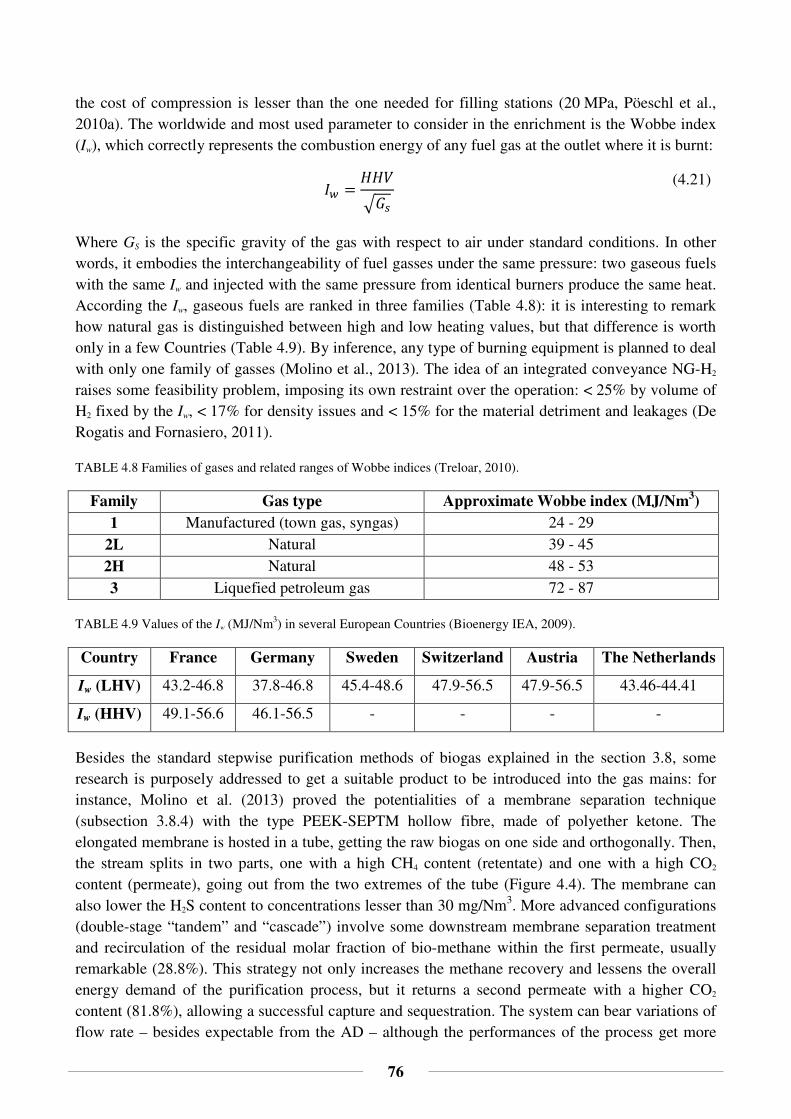
76

the cost of compression is lesser than the one needed for filling stations (20 MPa, Pöeschl et al., 2010a). The worldwide and most used parameter to consider in the enrichment is the Wobbe index (Iw), which correctly represents the combustion energy of any fuel gas at the outlet where it is burnt:

0± = ppa²�k (4.21)

Where GS is the specific gravity of the gas with respect to air under standard conditions. In other words, it embodies the interchangeability of fuel gasses under the same pressure: two gaseous fuels with the same Iw and injected with the same pressure from identical burners produce the same heat. According the Iw, gaseous fuels are ranked in three families (Table 4.8): it is interesting to remark how natural gas is distinguished between high and low heating values, but that difference is worth only in a few Countries (Table 4.9). By inference, any type of burning equipment is planned to deal with only one family of gasses (Molino et al., 2013). The idea of an integrated conveyance NG-H2 raises some feasibility problem, imposing its own restraint over the operation: < 25% by volume of H2 fixed by the Iw, < 17% for density issues and < 15% for the material detriment and leakages (De Rogatis and Fornasiero, 2011).

TABLE 4.8 Families of gases and related ranges of Wobbe indices (Treloar, 2010).

Family Gas type Approximate Wobbe index (MJ/Nm3) 1 Manufactured (town gas, syngas) 24 - 29

2L Natural 39 - 45 2H Natural 48 - 53

3 Liquefied petroleum gas 72 - 87

TABLE 4.9 Values of the Iw (MJ/Nm3) in several European Countries (Bioenergy IEA, 2009).

Country France Germany Sweden Switzerland Austria The Netherlands

Iw (LHV) 43.2-46.8 37.8-46.8 45.4-48.6 47.9-56.5 47.9-56.5 43.46-44.41

Iw (HHV) 49.1-56.6 46.1-56.5 - - - -

Besides the standard stepwise purification methods of biogas explained in the section 3.8, some research is purposely addressed to get a suitable product to be introduced into the gas mains: for instance, Molino et al. (2013) proved the potentialities of a membrane separation technique (subsection 3.8.4) with the type PEEK-SEPTM hollow fibre, made of polyether ketone. The elongated membrane is hosted in a tube, getting the raw biogas on one side and orthogonally. Then, the stream splits in two parts, one with a high CH4 content (retentate) and one with a high CO2 content (permeate), going out from the two extremes of the tube (Figure 4.4). The membrane can also lower the H2S content to concentrations lesser than 30 mg/Nm3. More advanced configurations (double-stage “tandem” and “cascade”) involve some downstream membrane separation treatment and recirculation of the residual molar fraction of bio-methane within the first permeate, usually remarkable (28.8%). This strategy not only increases the methane recovery and lessens the overall energy demand of the purification process, but it returns a second permeate with a higher CO2 content (81.8%), allowing a successful capture and sequestration. The system can bear variations of flow rate – besides expectable from the AD – although the performances of the process get more

77

affected by the inlet pressure: the higher it, the lesser the recovery efficiency, as the rise of the pureness of the retentate is not enough to offset the methane loss in the permeate stream. The need of a moderate inlet pressure in the purification stage implies the setup of an additional compression stage for the injection into the gas mains (1.6 MPa).

FIGURE 4.4 Simple sketch of the membrane separation type PEEK-SEPTM hollow fibre for pipeline-addressed biogas purification (Molino et al., 2013).

The injection of any gaseous stream inside the pipelines needs adequate knowledge about fluid dynamics, since not only the physical feature of the grid (roughness, diameter, length) affect its movement, but even its intrinsic properties such as density, pressure and viscosity. Since the high pressure of the gas, what is generally verified within the pipeline is the turbulence of the flow, represented by a Reynolds number Re > 4000. The assessment of the dimensionless friction factor f, an empirical quantity determining the pressure (energy) drops of the fluid along the pipelines, is the most important concern of many analyses, inasmuch as it affects the cost of the whole gas distribution system; as a matter of fact, the greater it, the greater the needed pipe diameter and thus the cost. There is a broad bibliography about the ways to compute f, although valid up to values of Re between 104 and 106: for higher values, normally verified within gas pipelines (Re = 106-107), those models expire. Morini et al. (2010) proposed the use of computational fluid dynamics (CDF) commercial codes so that to make up for the previous lacks and to run simulations with different gases. The thermodynamic properties of the gaseous mass are related each other thanks to an equation of state (EOS), which the literature is plentiful of. The easiest EOS considers the constancy of some properties like density and viscosity, and it can be successfully applied to a homogeneous blend of gases. Conversely, the well-known ideal gas EOS can be more broadly referred to a stated blend of low-density ideal gases, provided that one of the two following conditions are respected: low pressure (≈ 1 bar) and no matter the temperature or high pressure (>> 1 bar) and supercritical temperature. Anyhow, the most reliable EOS is the empirical one proposed by Redlich and Kwong in 1948, which considers the molecular size and the interactions among them, being valid up to the critical point and in the liquid-vapour condition. The aforesaid authors used this last model to compare the f of NG with the one of a promising team of fuels, such as two types of biogas (40% CH4 + 60% CO2 and conversely) and a blend of CH4 (90%) and H2 (10%). The imposed absolute roughness of the pipes and the boundary conditions (mass flow rate, temperature and turbulence intensity) were clearly constant for the four gases. In biogas, the presence of CO2 increased both the density and the viscosity, with an overall effect of increasing Re and lowering the pressure losses with respect to NG; the opposite behaviour is verified for the blend CH4/H2. Yet, f proved quite the same (0.019), making the economic evaluation of the pipeline impossible; this is the reason why the authors proposed an indicator, named energy specific toll (EST, formula 4.22), accounting for the most relevant parameters of the gas delivery (pressure drop and density). EST, properly the specific energy needed to transport gases, provides some indicative information about the economic benefits of the conveyed fuel: the lesser it, the more convenient its

78

transport. Although the most energetic blend CH4/H2 resulted as the least profitable one (ETSCH4/H2 = 2.86 × 10-6 m-1 vs ETSNG = 1.47 × 10-6 m-1), it is important to point out that EST depends on the length of the pipe (in the simulation L = 4 m), hence in the real cases the differences may become negligible.

%` = ∆x³ � 1d × dpa (4.22)

The health risk associated to the direct management of biogas by people (e.g. cooking) is another issue worth examining: it concerns not only the chemical, but even the microbial aspect, which is mostly suggested since the origin of the fuel. Naja et al. (2011) assembled a detailed bibliographic study and they finally proved that there are no risks arising from acute or chronic exposures to biogas vents while cooking, stemming from the lighting phase and from a failed combustion. It is no more valid when biogas derives from suspicious dangerous substrates (e.g. wastewater sludge and industrial waste), wherein extraordinary compounds might be present and a more detailed study must be done. The same authors provided a reasonable guideline for the assessment of the risks which is briefly reported in the follow-up. When a chemical substance does not own a recognised estimate of the concentration causing evident effects, expressed by the toxicity reference value (TRV), one has to make a qualitative analysis based on data from the literature. Otherwise, it is needed to compare the TRV with the expected concentration of the pollutant C(t) in a close environment with an emitting source (e.g. a stove in a kitchen), retrievable from the literature. The proposed formula (4.23) is worth assuming a perfect mixture of the substance in the air:

t(#) = ́a µ1 68¶¥· t�68¶¥ (4.23)

Where C0 is the initial concentration of the substance in the room [M L-3], V is the volume of the room [L3], λ is the renewal rate of the air [T-1], E is the constant substance emission rate [M T-1], t is the time when the source is switched off [T]. On the contrary, the microbial contamination is assessed from the amount of breathed in colony-forming units (cfu) during the exposure, which according to Vinneras et al. (2006) is highly diluted (10-100 cfu/m3

biogas). This is a pointless reckoning as far as cooking is concerned, since the volume of inhaled biogas is small (0.417 l), thus the possibility to receive even a pathogen is extremely rare.

Some final remark about the three most straightforward uses of upgraded biogas, explained in the previous sections, concerns the concealed weaknesses of the biogas implementation, such as the width of the distribution scale, the subsidies to the renewables and the social acceptance. According to Börjesson and Ahlgren (2012), the small-scale use of biogas, within the municipality where it is produced, suffers from stern restrictions, therefore no growth in the use is perceived with subsidies lesser than 60 €/MWhbiogas. A regional (middle-scale) use implies the construction of short distribution piping bringing to a rise in the biogas use when subsidies exceed 40 €/MWh. The third option is represented by the large-scale (national) transport of biogas cylinders with trucks: it is not as demanding as the former, since a large preliminary investment for the construction of the grid is not needed. Anyhow, the biogas utilisation shifts from the DH to the vehicle sector. The last possibility is the large-scale realisation of an expanded natural gas grid, which can be used by each municipality directly (pumping out or injecting), provided that a connection is available. The

79

successful and broad provision of gas for heating purposes implies high costs of setup, which become affordable if high subsidies are provided (60 €/MWh). The grid as a whole, sometimes incorporating already present NG grids, may thus provide NG along with biogas (co-distribution). The weakness of the system is that it is not properly planned for the biogas distribution, but for the natural gas, more plentiful till now: that is why it might enhance the dependence of the fossil fuels rather than promoting the diffusion of biogas, oppositely to the more suggested regional and truck distributions. What is important to understand is that the exploitation of the full biogas potentialities are often sternly restrained by the high costs of incentive from the Government: affordable outgoings can cover up to the 75% of the biogas potential at most. Furthermore, the greater the incentives, the more expensive the biomass which the biogas stems from: if cheap organic waste can be used when no financial supports are provided, energy crops can be processed too when the fuel demand and the incentives rise.

4.6. CHIEF ISSUES OF THE BIO-HYDROGEN MANAGEMENT

Like biogas, H2 has to be upgraded before the use as well, in particular when it is required in PEM fuel cells. When hydrogen is purified from syngas, the main hurdle is the content of CO which, even in small quantities, can sternly impair the Pt layer, which catalyses the H2 cleavage: this reduced activity, called poisoning, is stood up to concentrations below 1 ppm. Thus, a first coarse removal of CO (till 1%) with the water-gas shift reaction (formula 4.3) – increasing the H2 content too – has to be integrated with a further oxidation. A successful, but still under refinement technology for the attainment of the same goal is embodied by different kinds of membranes, employed either for the generation of a pure O2 stream for the oxidation stage, or for the selective withdrawal of CO and CO2. A widely discussed barrier to the large-scale implementation of the “hydrogen economy” concerns the storage, in particular in the transportation sector. The aforesaid easiness in storage H2 has to deceive no expectation, since it is true when considering an energy content on a weight basis (threefold petrol), but not on a volume basis, so much so that acceptable haulage performances can be achieved with unfeasible equipment. Furthermore, correct equipment must store and deliver the fuel in any weather condition, both icy and hot, and aptly, that is, complying with the operative functioning conditions (pressure and temperature). Nowadays, the state-of-art is still on incomplete solutions, unviable in terms of energy density and release rate (De Rogatis and Fornasiero, 2011). The most widespread strategy to increase the energy density of gaseous H2 employs high-pressure steel cylinders (till 300 bar), whose integrity and cost of compression are the two greatest barriers to overcome. Research on that topic and good pioneering tests with fibre-reinforced composites compressed tanks proved performing up to 700 bar in transport applications. In such devices, normally cylindrical, it is possible to identify three shells, inwardly: an anti-impact reinforcement, a light (carbon fibre) gas pressure load-bearing layer, and finally a H2-impermeable coat. Despite the amount of endeavours on this topic, there are still unsolved safety and freezing issues concerning the compression, besides the expensiveness. Already on place H2 storages were realised underground, either in buried tanks (as compressed gas or liquid) or in geological frames such as depleted gas field, aquifers and salt domes. Once the geological features were proven suitable, this system offers the possibility to keep huge quantities of fuel, so that to meet irregular demands for a long time. A more insightful way to increase the energy density per unit of volume, which would enhance the haulage, is the liquefaction up to 20 K

80

and at patm. At once, it grants longer ranges than gaseous H2 to vehicles burning it, so much so that it has already been applied for busses in Germany. Actually, the liquefaction not only takes the 30-40% of the H2 energy up, but it arises several safety issues, forcing the avoidance of some devices (electrical equipment, static electricity, flames, hot items) where liquid H2 is handled (fuelling stations, transport vehicles…). Furthermore, relentless high-pressure losses of gaseous H2 (boil-off) during the vessel loading have to be either released into the atmosphere through safety valves or somehow valorised. The last studied option concerns the solid form, that is, H2 molecules stored inside a support material or chemically bound to it, but eventually released. Research is addressed to find an economically viable way to accomplish this function, concerning not only the support itself (e.g. regeneration, resistance to impurities), but even the amount of storable H2 and the quickness of release. Taking into account its properties, atomic H2 may form alloys (metallic or interstitial hydrides) when it is absorbed within the crystalline frame of a metal (e.g. Pd); the heating of the material triggers a sudden rescue of gaseous H2. Similarly, it may electrically interact with a solid surface (adsorption) and, according to the energetics of the operation, it can be either a physisorption or a chemisorption. The first grants faster adsorption/desorption cycles, while the second, characterised by the formation of chemical bonds, can take more gas up, but irreversibly impairing the support. Experiments on the coupling of the two adsorptive ways proved a higher efficiency (as weight percentage) than single processes. Being a superficial phenomenon, it is clear that the adsorbing medium must have large free surfaces, i.e. being highly porous or nanoporosus, like zeolites, metal-organic frameworks (synthetic structures made of stiff organic molecules and metal ions) and carbon-based materials (grains, AC and AC fibres). Eventually, it is possible to exploit some compounds able to chemically react with and release gaseous H2 reversibly. The main hurdle in the transportation sector is the unfeasibility to regenerate the original storing material on-board the vehicle owing to insufficient temperature and/or pressure variations. At once, the possibility to deal with regenerative cycles, far less energy demanding than compressed hydrogen, is a greater and safer advantage. Liquid hydrides rescue the H2 content at lower pressure and temperature conditions than solids and that is the reason why they are often more preferred. The most widespread compounds for this purpose are magnesium hydride (MgH2), displaying good storage efficiencies (up to 7.7%), sodium aluminium hydride (NaAlH4) and sodium borohydride (NaBH4), reacting as stated in formulas 4.24-4.26. Alternative and maybe more immediate approaches are based on the use of highly hydrogen-containing compounds, like hydrocarbons, ammonia, methanol and glycerol (subsection 4.1.2). Finally, more advanced research is focused on the storage skills of doped polymers (e.g. titanium-decorated ethane-1,2-diol), capillary arrays and micro-balloons, also called hollow glass microspheres (d = 10-300 µm).

The delivery cost from the production site to the end users affects hydrogen as well, maybe more than bio-methane owing to the aforementioned storage issues. Generally, the need of a branched and differentiated distribution network pushes the reliance on more than one delivery fashion, able to equally ensure a safe and unpolluted storage (De Rogatis and Fornasiero, 2011). Even in this case pipelines look like the best candidates for that purpose, since accomplishing both the functions of

MgH� + 2H�O → 2H� +Mg(OH)� ∆H < 0 (4.24)

3NaAlH� → Na�AlH: + Al + H� ∆H > 0 (4.25)

NaBH� + 2H�O → NaBO� + 4H� ∆H < 0 (4.26)

81

storage and delivery, as already explained. Despite some kilometres of H2 mains have already been realised (720 in USA and 1500 in Europe), one has to recognise that as a long-term strategy, suitable when the transition toward the “hydrogen economy” is already mostly developed. As a matter of fact, it is unconceivable to face in a short time span the cost of a new hydrogen pipeline, also depending on the location, from the cheaper countryside to the more expensive urban areas. So, a first push toward the virtuous “hydrogen economy” is surely the conveyance via trucks, ships and trains: if on one hand it offers the possibility to use solid H2 carriers, unviable in pipelines, on the other hand it involves the aforesaid great energy consumptions and losses problems. A successful and quite cheap strategy is offered by the conveyance of a blend of NG and H2 (up to 20%) along the already existing gas mains, which have to be modified surely, but not as much as in the case of greater H2 shares. This strategy, already discussed in the previous subsection and however more expensive in terms of specific energy spent to transport the gas, can be particularly convenient for hydrogen refuelling stations provided with gas separation equipment. A CH4 reformer may be another good idea as well, unless it becomes an intense source of not-catchable CO2 emissions. Similarly, it is the transportation of ethanol as liquid H2 carrier, thus with less problems of transport, but needing a later conversion into H2, e.g. within suitable refuelling stations.

4.7. LIFECYCLE ASSESSMENT AS KEY TOOL FOR ENVIRONMENTAL EVALUATIONS

The knotty opening on market of any biofuel is sometimes accompanied by issues raised by the difference, often remarkable, between their costs of production and implementation, and the actual environmental benefit they can provide. The most ubiquitous tool for the appraisal of the environmental burdens of any marketable good throughout its lifetime is the lifecycle assessment (LCA). It is important to specify that the outcomes of any LCA crucially hinge upon the available data and the (reasonable) assumptions, including the boundaries of the system: therefore, one does not have to consider them as the truth, but as reliable inferences. Normally, those results are summarised with more or less direct indicators, whose achievement is stated by different methods (e.g. Ecoindicator 99). Midpoint indicators (MPI) correspond to well-known problems, such as rains acidification and global warming, while endpoint ones (EPI) try to extend the effects of those physical quantities so that to represent the final drawbacks on the human health, the resources and the ecosystem quality. Eligible procedures of normalisation of the EPIs and aggregation of the lasts are often carried out, with the ascription of weights chosen according to the earmarks of the contest; the goal is the achievement of a unique score roughly displaying which is the most impacting solution. In the follow-up, some noteworthy LCA from the literature are presented and discussed; when dealing with the environmental impact of transport fossil fuels, LCAs are properly named “well to wheels”. The different environmental friendliness of 1 MJ of grid-injected natural gas and biogas from the mono-fermentation of energy crops was compared by Jury et al. (2010). The study raises not only the well-known problem of food grown for energy purposes, but even the strong impacts of farming activities. The general results stated that the biogas scheme is more damaging than NG in terms of human health and ecosystem quality, whereas (quite obviously) less in terms of resources consumption and climate change. That fact is not so astonishing, since the huge quantities of mineral fertilisers (e.g. NO3NH4 and P2O5), the use of diesel-fuelled machines for sowing, tilling and harvesting and the occupation of areas otherwise addressed to the food production, with the ensuing necessity of importations. Therefore, it is evident that the chief issue of biogas production is

82

farming, more than the assumed upgrading, compression at 0.8 MPa, injection with a small percentage of LPG (3.705% Nm3/Nm3) and distribution along a pipe being 5 km long. Milder impacts could be considered if the fertilisers were partially replaced by the liquid and the solid digestates, which in the analyses were regarded as neutral-impacting matters (neither troubling waste nor profitable nourishment). The final balance, with the one-score method, proved to the detriment of biogas with respect to NG: of course, it was remarkably affected by the choice of the weights, suggested by the Ecoindicator 99 (human health: 40%; ecosystem quality: 40%; resources: 20%). The figures of this LCA are surely questionable but reasonable, hence they have to be used as indicative tools of the weaknesses of the biogas production from energy crops, which have to be improved, and where it is more expedient to focus research and economic resources on. Moving to the transport sector, Patterson et al. (2013) carried out a LCA on 1 km of run distance (functional unit, FU) by vehicles fuelled with fossil diesel and with two types of biogas. One is CH4 from a single-stage (AD) and the other is CH4/H2 from two-stage (DF + AD) process, attained both from food waste (FW) and from wheat feed (WF), and both refined within a PSA unit. Those classes of substrates coarsely summarise the main source for AD processes, that is, MSW and energy crops/food waste: moreover, WF proved to be particularly hydrogen-fruitful (Hawkes et al., 2008). As far as the results are concerned, fossil diesel is more environmentally impacting than the FW-derived bio-fuels, owing to the cheapness of the feedstock and the avoidance of a landfill disposal. On the contrary, WF-derived bio-fuels are more harmful than diesel, although the consumption of fossil fuels and the impacts on the climate are comparable. Single-stage biogas is more energetic than two-stage one when FW is used, oppositely to the WF setting, where blend CH4/H2 prevails over the CH4 despite the lesser H2 content than with FW (2% against 20%). As it seemed as obvious, remarkable differences were present according to the type of feedstock; anyhow, it is likely that more suitable technologies and digestion fashions (e.g. co-digestion with manure) improve the overall CH4/H2 yield. A similar study performed by Browne et al. (2011) compared the costs and the potentialities of bio-methane as vehicle fuel from different sources in Ireland: all the quantities were referred to as litres of diesel equivalent (lde). Despite the all three solutions resulted competitive against conventional petrol and diesel (1.38-1.45 €/l), the cheapest one was the digestion of OFMSW (0.36 €/lde), mostly because fostered by high gate fees on waste (70 €/t) which are, however, changeable. Then, the digestion of SHW (0.65 €/lde) and the co-digestion of grass and dung (1.40 €/lde): this last one must not be neglected, albeit expensive, as a plentiful local resource and even able to exceed in and of itself (15.5%) the compliance with the national renewable energy share in transport (RES-T) before 2020, imposed to 10%. Yet, the respect of that target would increase the price of bio-methane up to 1.28 €/lde, not only greater than CNG (0.71 €/lde), but also than petrol and diesel. Therefore, the best strategy for the joint respect of the RES-T and the valorisation of bio-methane might be the bio-CNG (0.82 €/lde), a blend made of CNG (80%) and bio-methane (20%). Another lesser opportunity, studied by Lacour et al. (2012) in France, is provided by the farming sector, where the aforesaid environmental problems can be partially worked out by implementing bi-fuel tractors (diesel + bio-methane) instead of only conventional diesel: moreover, if the fermenters are located near to the farm, a very short fuel path can be achieved as well. The authors assembled a thorough survey of all the complications related to the actual impact of bio-methane, by merging a standard LCA with a carbon balance, so that to assess the GHG emissions in terms of CO2 equivalent from each giving off source. It is consistent with the LCA guideline, but more addressed to the climate change and the energy dependence, as well as consistent with the

83

ISO14064 standard, the GHG Protocol and the 2003/87/EC Directive for GHGs emission allowance trading. They proved that both the pollutants emissions and the average efficiency of both types of engines are comparable, therefore complying with the emissions standards for the chosen type of tractor. Savings of CO2 at the end-use stage may reach 80% if the biogenic nature of bio-methane is considered. At once, they point up the radical differences arising according to the done assumptions: for instance, each assessment (carbon and energy balance, environmental impacts) is to the detriment of biogas than diesel, when the impacts from fossil fuel depletion (FFD), the biogenic nature of biogas, the control over CH4 vents and the recovery of flares were neglected. The results, expressed as the quantity of mechanical energy needed for agricultural operations (equivalent of run distance for cars) are 531 gCO2eq/MJ (bio-methane) vs 324 gCO2eq/MJ (diesel). Considering the biogenic nature of biofuels (according to the aforesaid Directive), bio-methane drops at 215 gCO2eq/MJ, getting null considering the further amount of avoided methane as GHG from uncontrolled AD in landfills. Nevertheless, all the costs and the emissions related to the biogas production (e.g. purification and compression) are significant, as well as the potentialities thus, stemming from the optimisation of the whole process (e.g. avoiding the CH4 losses of the process and storing the flaring-addressed biogas). A more specific well-to-wheels study was undertaken by Bordelanne et al. (2011), considering hybrid and not methane-fuelled cars compared to hybrid petrol-fuelled ones; in this case, the lifecycle of each fuel was throughout studied (production, transport and use) and the impacts of infrastructures and cars neglected. The resulted higher environmental performances of bio-methane from OFMSW were consistent with Browne et al. (2011), followed by energy crops, whose lifecycle “emits” more GHGs; moreover, the GHG emissions were far lesser than the limits of the Directive 2009/28/EC. Patently, the impacts dropped more or less remarkably in the hybridised versions. Yet, the remarkable environmental benefits stemming from the use of bio-methane-fuelled engines in an end-use analysis (-80% GHG emissions with respect to a petrol engine) dramatically decline if the upstream (or well-to-tank, WTT) branch of the process is considered. Anyhow, the likely implementation of particular gas engines (burning a lean CNG blend) may endorse the diffusion of natural gas blended with 70% volume of not upgraded biogas, abating the costs and the emissions of advanced treatment.

Once shown the different solutions for a right use of biogas, one may wonder which the most beneficial one is absolutely, under economic and environmental terms. A reasonable answer to this tricky issue was given by Uusitalo et al. (2013), who employed the LCA again, but rightly limited to the end use and distribution of the upgraded biogas in Finland. They considered three circumstances, each of which introducing a renewable aspect in the baseline scenario, made of a large-scale NG-fed CHP plant, fully petrol and diesel-fuelled vehicles and a local heating plant processing a blend of substances (40% NG, 20% biomass, 20% peat and 20% oil). The results were discussed in terms of produced energy, incomes (without costs), payback period, quantity and cost of reduced CO2 emissions. Without taking subsidies into account, the most convenient strategy is the utter replacement of fossil fuels with biogas in the transportation sector. However, the presence of a feed-in tariff makes the previous scenario economically comparable to the one wherein the CHP plant is supplied with only biogas, and a share of the generated power feeds a few vehicles; it is a clear example of the importance of political decisions, which may favour less environmentally friendly strategies. The last situation, where biogas supplies the heating plant and the electric energy partially supplies the vehicles, results as the least convenient, due to the choice of conservative

84

assumptions about the use of the generated heat (only three months per year). Anyhow, the potentialities of the biogas in the transportation sector are clear, also favoured by the next introduction of a sterner class of EURO 6 diesel vehicles, which have to be endowed with expensive reduction measures over NOx emissions, lesser when biogas is burnt. Oppositely, Patterson et al. (2011) proved that CHP plants able to recover at least the 80% of the generated heat are the most environmentally friendly solution for biogas. The LCA they undertook used as functional unit a stated amount of OFMSW produced in Wales able to return biogas, while the ranks of damage assessment were the three suggested by the Ecoindicator 99 (displacement of conventional resources, human health and ecosystem quality). The different scenarios were additionally considered in the centralised and distributed infrastructure, according to the reality they have to been applied in. The diversity between these two configurations, actually not so remarkable, suggests that the design of biogas plant distribution should be done apart from the reduction of transport needs, chiefly considering economic and practical aspects. The best solution previously explained is furthermore compared with a CHP plant without heat recovery which, in turn, proved the worst alternative. The strength of this system is not only the huge amount of recovered heat, but even the more thorough operative and emission controls than any end-use. For instance, despite the flexibility of use, biogas for domestic heating is not so positive globally, since having the same emissions of the baseline scenario where NG was burnt: the only benefit concerns the preservation of the fossil resource. On the contrary, in the transportation sector the replacement of petrol and diesel with the greener bio-methane is more beneficial, even considering the impacts of the vehicles themselves, differently from Bordelanne et al. (2011). Nonetheless, in both cases one has to consider the impacts due to gas vents during the upgrading and further costs (e.g. compression) which lessen the convenience.

4.8. CASE STUDIES: GERMANY AND CHINA

As far as biogas is concerned, Germany represents the most technologically skilled Country in the European Union, with more than 4000 plants and 500 manufacturers, employing up to 10000 workers. It is maybe the most important example of Country where the radical shift from conventional energy sources (e.g. fossil and nuclear) to renewables is taking place: the gradual transition begun not long ago (2010) aims at granting an electricity supply from renewables close to 80% before 2050 (Szarka et al. 2013). Electricity is a ticklish subject, because on one hand it is the most flexible and easiest way to convey energy, but on the other hand its nature prevents it from being stored in large quantities. This is a heavy limitation, since the energy demand is never constant over the time (both at daily and at seasonal scale) and it is particularly difficult to foresee its sharp swinging. The most widespread way to face this problem is to define a “base load”, namely a steady share of power, which to sum extra peak loads to. Unfortunately, given the well-known changeability of the renewables (e.g. wind and sun), it is difficult to apply this scheme, whose extreme consequences are represented by both the lack of enough energy or the sale of the surplus with a negative price. The overall improvement of the electricity supply is a demanding challenge which can be faced both with an advancement in the forecast of the energy demand and with control reserves, which are fluctuation-controlling power stocks with a capacity (MW) and a time at which they start up after the deviation demand-supply (30 s, 5 min and 15 min). This somewhat ambitious goal, needing advanced technological developments, is strongly fostered by a favourable legislation. For instance, the Renewable Energy Sources Act (EEG), issued in 2000,

85

subsidises renewable plants, granting incentives to biomass-fed ones (but wood fuel) feeding the electricity grid for 20 years; actually, the subsidy yearly drops (1%), so that to prod the plants to become more and more self-sufficient. The amendment of 2009 kept plants greater than 20 MWel out of the mechanism, in order to promote the setup of small-scale decentralised plants upon large-scale ones. The amendment in 2012 prodded biogas-CHP-units to join the “flexibility premium”, a type of extra funding for demand-based power suppliers; moreover, since 2014, each biogas plant with a capacity exceeding 750 kW is forced to take part to this mechanism. Further incentives were given to technologically innovative plants, with CHP and processing only renewable raw materials (RRM): plants using non-renewable feedstock are prevented from requiring this bonus. Additionally, the control reserve market, previously covered by fossil-based power plants, has been opened to bio-methane-based ones too. Along with renewables, Germany is pursuing another ambitious goal aimed at nullifying MSW within 2020: it cannot, obviously, be reached with only AD facilities, whence the need of a careful integrated strategy. Gate fees for waste disposal via AD processes are the lowest compared to composting and incineration: these three options compete among them for the feedstock, even if the last two are more levied than AD, as the higher amount of CO2 they give off.

As the most populated and important developing Country, China’s contribution to the conversion of organic substrates to biogas is remarkable, besides the consequent reduction of fossil fuels for cooking, lighting, heating and chemical fertilisers. The background wherein the setup of medium and large-scale biogas plants should take place is somewhat complicated. On one hand, both farming and animal husbandry sectors are managed by individual holders after the economic reform of the early Eighties, with an increased fruitfulness. On the other hand, the incorrect handling and collection of the organic remnants from those sources and from the growing urban areas, partially due to people’s lack of knowledge and awareness of their potentials, leads to stern environmental problems of land occupation (landfills), air, water and soil pollution. Furthermore, the vastness of the Country is related to deeply different climates, therefore types of crops and efficiency of conversion (Jiang et al., 2011). The total replacement of high-carbon-containing fossil fuels with slighter ones, up to actually renewables, is to be hoped and partially already established in many household services (e.g. LPG or NG instead of coal). Owing to the willingness of the Government in terms of favourable energy, economic and environmental policies, some reparation measure is being taken, mainly related to the recovery of landfill gas and the setup of the aforesaid suitable fermenters for the production of biogas from many sources, such as crop straw (rice, corn and wheat) and animal dung (pig, cattle and poultry). In the past years, the strong subsidies given for the construction of anaerobic digesters were not supported by further ones for their maintenance. That fact, along with a widespread disinterest of single farmers in investing money in biogas recovery, is the reason of the recklessness of the already implemented small-scale plants. The concrete vessels, often underground, are devoid of almost any type of control system (e.g. temperature, stirring), thus dependent of the weather conditions, very changeable throughout China. The future perspectives about that, pushed by sterner and sterner environmental policies, concern the installation of modern large-scale plants, where the broad capacities, along with more advanced technological equipment, might increase the overall biogas production. At once, those plants need skilled workforce, thus job opportunities, regardless of the more advanced mechanisation, which, instead, provides more safety; unfortunately, it might also become a costly barrier for the diffusion of such plants.

86

5. NEW HYBRID POWER PLANT

PROPOSAL

This chapter tries to summarise a few aspects tackled during the previous dissertation, inquiring into the potentialities of a possible application that the biogas might have. It briefly concerns the exploitation of its heating value for the natural gas catalytic thermal decomposition, a process needing a rather important amount of thermal power to happen. That helps the fossil resources decarbonisation and the involvement of the renewables as the chief hinge of the energy supply chain. The proposed hybrid power system is compared with a conventional combined cycle gas turbine system (CCGT), fed by bio-methane, by energetic and economic standpoints. All the computational details are reported at the end of the chapter.

5.1. NEED TO INTEGRATE RENEWABLE AND CONVENTIONAL ENERGY RESOURCES

One of the problems concerning the AD implementation appeared in the former treatise, is the difficult access to the market due to the still powerful fossil fuels. If on one hand some study proved the economic competitiveness of bio-methane on petrol and diesel, on the other hand it cannot prevail over CNG yet. Then, this situation gets worse if incentives to the renewables are removed and if stringent renewable-implementing targets (e.g. the European RES-T) are respected. The only successful way to overcome these economic hurdles is blending bio-methane with CNG (bio-CNG), thus looking for cooperation and not conflict between the conventional and the renewable sectors. Of course, bio-methane may rightly inherit all the already available large technological assets of the natural gas (e.g. CHP engines and vehicles), while bio-hydrogen can growingly assist it with some more advanced equipment (e.g. fuel cells and hydrogen gas turbines). Along with the difficulty to devise performing ways for the quick and virtuous diffusion of bio-methane and hydrogen worldwide, one considered the gasification and the catalytic reforming, not only for the treatment of biogas (DR proved the most suitable strategy), but also for the aimed management of the traditional fossil energy sources. For the sake of example, it is maybe worth comparing the costs of production of H2 and the related net emissions of CO2 shown in Figure 5.1, which more straightforwardly gives an idea about a likely short-term solution. It is clear how the concept of carbon capture and sequestration, sparsely hinted along the dissertation, appears as the main CO2-abating technique, able to turn a heavily emitting GHGs source (coal industry) into a “green” manufacture. Thus, one may soundly believe that, given the present impossibility to implement both cheap and environmentally friendly technologies, the short-term energetic future is likely to be ruled by the compromise consisting in the advanced integration of renewables and more wisely used fossil resources. A similar idea was caught by Hirsch et al. (2001), who stated the importance of solar energy with those words:

87

“There is a pressing need to develop greenhouse gas mitigation options that can be applied to fossil

fuels in the mid-term. Endothermic processes that use fossil fuels exclusively as chemical reactants

and solar energy as process heat yield cleaner fuels with a solar-upgraded calorific value. Thus,

the mixing of solar and fossil energies could substantially reduce greenhouse gas emissions and

become an important intermediate solution towards a sustainable energy supply system.”

FIGURE 5.1 Hydrogen production costs (left) and related CO2 emissions (right) (Winter, 2011).

The underground storage of CO2 is sometimes regarded to as unsafe for the environment and for people, due to some unexpected leakage and migration polluting the atmosphere and acidifying both aquifers and oceans (Damen et al., 2006), as well as really unable to compensate for the global emissions: 8200 TgCO2/y is the CCS target for 2050 [2] against the world’s production of 30000 TgCO2/y [3]. That is the reason why, before considering the sequestration, it is reasonable to valorise the amount of available carbon. At once, as gaseous CO2 is even difficult to manage, one may also consider the attainment of solid graphite from the pre-treatment (cracking) of fossil hydrocarbons (formula 4.10 for methane). That allows the production of gaseous H2, which can be fruitfully associated with electricity generation (Gibbins and Chalmers, 2008), e.g. feeding high-temperature molten carbonate fuel cells (MCFC), for the combined generation of power and heat (De Rogatis and Fornasiero, 2011). This highly efficient strategy, thanks to its straightforwardness, might make up for the unavoidably lesser net available energy of the process (lesser LHV of the treated fuel and energy spent for the cracking) with respect to the widespread post-combustion capture technique. Yet, regardless of this loss, the pre-combustion cracking not only does not suffer from additional costs of storage – and the difficulty to find a suitable place for the purpose – but in fact it benefits of earnings from the sale of the generated graphite. Among the multifarious market opportunities this by-product may have (after some refinement of course) one considers: carbon nanotubes and carbon blacks, with remarkable electrical conductivity, sorption and antistatic skills (use as sorbent material, soil conditioner, filler in rubber, fibre feedstock, addictive in steel, catalyst support for methane cracking), besides the conversion to graphene in order to get electronic, sensing, energy equipment (Zheng et al., 2010). Extra quantities of solid carbon can be quite easily stored as energy reserve for the future as well. Despite the hydrocarbon cracking is a quite evocative process, it is highly energy-consuming and, as already highlighted by some author (Hirsch et al., 2001; Assabumrungrat et al., 2012), one had better employ renewable energy sources to give it the needed “green” heat power. As a matter of

88

fact, the complete process takes places at very high temperatures (up to 1800 K for methane), which can be remarkably lessened (to 1150 K) when metal catalysts are used (Croiset et al., 2011). Unfortunately, the simplest regeneration of such catalysts implies the oxidation of the settled solid carbon particles, being the mechanical removal generally hard and not fully successful, at least at high temperatures (Abánades et al., 2011). Nevertheless, fluidised-bed reactors with carbon-based catalysts do not show that setback and they can efficiently work with relatively low temperatures (up to 1123 K, according to Muradov, 2000). The following paragraphs describe the hinted carbon-free energy chain, comparing it with a traditional CCGT cycle by an energetic standpoint. On the other hand, some economic analysis is carried out in the final section.

5.2. SYSTEM LAYOUT

The general plant layout (Figure 5.2) is organised according to already existing parts which were studied by different authors separately; by referring to their work, it is possible to consider reasonable technologies and features explained in the follow-up and enlisted in Table 5.1.

Thermo-catalytic decomposition unit, TCD (Muradov, 2000). It is a fluidised-bed reactor with catalytically active carbon particulates where the natural gas cracking takes places at atmospheric pressure and a temperature in the range 800-900°C. The preheated NG (400-500°C) enters the bottom of this unit and it moves upward, meeting a finely-ground blanket of active carbons (AC, d < 20 µm) fostering the conversion at relatively low temperatures and in a quite short time (1-3 s). It is clear that this scheme resembles the fluid coking (FC) process, but for the higher operative temperatures (850 vs 550°C) and the lighter hydrocarbon feedstock. Being this residence time not enough for the full conversion (50%v), the blend of exhausted gasses is filtered with a gas separation membrane (M), returning high-grade hydrogen (99%v) and flue hydrocarbons to be recycled. The presence of unburnt species (unsaturated and aromatic hydrocarbons) in these gasses or sulphur-containing compounds in the fuel does not impair the process; in fact, the AC catalytic properties are improved (internal regeneration of the catalyst). That is a very positive and robust feature of the system, allowing the management of rather raw hydrocarbons (crude oil) and saving money in their pre-treatment. Moreover, the thermal decomposition is more energy-demanding and less hydrogen-efficient for NG than for other heavier hydrocarbons (propane, butane, petrol); this is why the extension of this process is straightforward. The settlement of NG-derived carbon particles on the active carbons not only increases their volume (up to d ≈ 100 μm), but it also lessens their surface and it worsens the catalytic skills. This is why an active carbon recycling circuit is needed, which externally accomplishes their regeneration after 6 h of direct exposure to NG. However, it is important to point up that 20-30% of the carbon is recycled, while the chief part can be further treated or directly sold as marketable commodity. The catalyst flow is gathered from the bottom of the TCD unit and, after the partition, sent to a grinder (G) where the original size is retrieved. Then, it is moved to a heater (H) where it is treated with gasses at 900-1000°C (mainly CO2, O2 and H2O) thanks to which it recovers the catalytic properties (surface gasification). The heater is often fed with NG combustion products, but it can be successfully replaced by biogas, annulling the GHG emissions of the process and providing suitable oxidising agents (CO2). Moreover, that allows some money and energy saving in the biogas upgrading process.

89

Molten carbonate fuel cell, MCFC (De Rogatis and Fornasiero, 2011). This unit (F) receives the upgraded H2 from the TCD unit, returning electricity with a high efficiency (0.45-0.60). Although this equipment is not the most efficient – Direct Carbon or Magnesium-Air fuel cells can reach 0.8-0.9 of efficiency – it is well-established, broadly available on the market and object of much research. Moreover, it offers several advantages, among which the resistance to poisoning from impurities (PAH, CO, sulphurous compounds) and large-scale capacities (> 1 MW). The feasibility of coupling TCD with MCFC units has already been proved by Muradov (2003a). The cell often operates at environmental pressure and high temperatures (up to 700°C). High-purity H2 enters the anode side of the cell and it is split in two protons and electrons. The latter ones are caught by an electrical circuit ending in the cathode, where they meet atmospheric O2 and recycled CO2, forming carbonate ions. This compound migrates to the anode where it reacts with the said protons, giving rise to flue water and CO2:

Cathode side tc� ;�c� → tc��8 268 (5.1a)

Anode side p� tc��8 → 2p_ 268(tothecircuit) tc��8 → p�c tc� (5.1b)

Overall p� ;�c� → p�c (5.1c)

Gas turbine, GT (Massardo and Bosio, 2002). A few studies have already been done about the exploitation of the hot MCFC flue gasses (H2O, N2, O2) in thermodynamic cycles. In particular, the quoted authors claim that a bottoming combined cycle gas turbine (CCGT) can increase the overall plant electrical yield up to 69%. A GT unit (A) downstream the MCFC can lower the flue gasses enthalpy with noteworthy electricity production. Of course, such gasses are supposed to be at a sufficiently high pressure level (≈ 350 kPa) so that to expand; this not only requires additional compression energy inputs, but also could disrupt the kinetics of the upstream process. However, the NG TCD efficiency is perceptibly impaired only at high pressure levels (170 kPa, Croset et al., 2011), while no criticality is recorded for MCFC. It is therefore reasonable to use pressurised NG without accounting for further efficiency losses. Heat recovery steam generators, HRSG (Massardo and Bosio, 2002). It is a multistage device, made of three counter-flow heat exchangers (economiser E, vaporiser V and superheater S), where both the GT and the biogas flue gasses transfer their high enthalpy to looped water circuits. The produced steams are then sent to two steam turbines, whereas the flue gasses at T = 108°C (197°C in the second case) may leave the system definitively (stack gasses). It is clear that their relatively small residual enthalpy can be still successfully employed in organic Rankine cycles (ORC) for the further electricity production, or in a cogeneration system for the waste heat recovery. Those solutions, not applied here but strongly hoped indeed, would optimise the use of resources, as well as increase the overall plant efficiency. Steam turbine(s), ST (Massardo and Bosio, 2002). This one pressure level unit (B) yields electricity from the waste heat of both the GT and the TCD. Being the flue gasses enthalpies different, the thermodynamic coordinates of the ready-to-expand steam are different each other accordingly. Yet, one tried to be as consistent as possible with the reference work, thus the temperature and the molar rate are the only changed parameters. In particular, the second turbine works with a less molar rate but a higher expansion temperature than the first one, because of the small amount of high-temperature biogas flue gasses.

90

Last but not least, there are auxiliary pieces of equipment adjusting and completing the previous plant layout. It is worth quoting a gas membrane separation unit (M), where high-temperature TCD gasses are split in the two chief streams: high-purity H2, sent to the MCFC, and unconverted hydrocarbons (mainly CH4, but also PAH), recycled to the TCD inlet pipe. Due to the high temperature of the inlet gasses (≈ 850°C), this unit is made of ceramic material. Prior to enter the MCFC, the H2 stream crosses a heat exchanger (D) aimed at the joint temperature lessening thereof (up to 700°C) – which could damage the MCFC otherwise – and NG preheating. The plant is also given input energy by a few compressors (C, for air and biogas) and pumps (P, for water). Such energy, to be subtracted from the gross plant electricity production, must be enough to let the fluid overcome energy losses due to friction or disruptions.

5.3. ENERGY ANALYSIS

Prior to considering the studied energy system, one inquires into the energy needs of the bio-methane production by means of a simple energy balance (Table 5.2). This amount of energy is later accounted for the assessment of the energy efficiency of the whole process. Considering a middle-scale MSW-fed biogas plant (10000 - 20000 t/y of waste), one assumes reasonable collection and transportation distances of 12 and 4 km (20% less than the reference author’s proposal), a biogas energy content of 6.6 GJ/tDM, and a biogas yield equal to 308 m3/tDM (Pöeschl et al., 2010a). The assumed operative costs concern the feedstock pre-treatment, the electricity and heat consumption and the biogas upgrading (through membrane technology). As far as the digestate management is concerned, it is reasonable to limit the costs to a few operations (screw press separation, loading, transportation for 15 km and field spreading of the liquid and solid fractions), so not taking into account the far more expensive drying and composting. As a matter of fact, the amount of digestate from large-scale biogas plants cannot be withstood by the soil, since the exceedance of its nutrient uptake capacity (Pöeschl et al., 2010a). According to the done premises, the bio-methane production energy consumption is equal to 18.30 MJ/m3

BIOCH4, being more than half of its LHV worth (33 MJ/m3 or equivalently 780 kJ/mol). On the other hand, the biogas one is far less than the former (9.78 MJ/m3

BG over a LHV = 19.8 MJ/m3BG), basically owing

to the savings on the upgrading process and the noteworthy presence of CO2 (40%v). The second part of the energy study deals with the performances of the already described hybrid energy system. It is important to state that this work is based on literature data not only in terms of equipment, but also in terms of energy yields. This is why it is judicious to carry out a preliminary backward analysis, where the equipment yields are retrieved, and then a forward analysis, where the energy production and overall efficiency are assessed reliably. All the following computations are expressed with an integral formulation rather than a linear one, due to the wide temperature ranges. As quoted before, the final tables report all the assumptions and computational details.

Heat recovery efficiency: T1 is the really reached temperature of the hot stream, T2 is its early temperature and T3 the early cold stream temperature.

l¹¢ = ∆p¥¢*�kºm¢¢m'∆p¥¢*�kºm¢*g°m =® �¹5»5¼ ½¾,¹(`)!`® �¹5»5¿ ½¾,¹(`)!` =

® µ∑ �h(vh Àh` ½h`� !h`�)¹h ·5»5¼ !`® µ∑ �¨µv̈ À̈ ` ½̈ `� !̈ `�·¹̈ ·5»5¿ !` = 0.84

(5.1)

91

Compressor isentropic efficiency: pf and pi are the downstream and the upstream pressures, while cv and cp the gas specific heat at constant volume and pressure respectively.

l¯ = º̀,hkm h̀º̀,¢m*° h̀ = h̀ÂwÃ8;Ã y h̀

º̀,¢m*° h̀ = h̀ Äwxºxh y;8¯Å¯�� 1Æ

º̀,¢m*° h̀ = 0.81

(5.2)

Gas turbine isentropic efficiency:

lj¥ = h̀ º̀,¢m*°h̀ º̀,hkm = h̀ º̀,¢m*°

h̀ h̀ÂwÃ8;Ã y = h̀ º̀,¢m*°h̀ Ä1 wxºxh y

;8¯Å¯��Æ= 0.89

(5.3)

Steam turbine electric efficiency: ηp and ηal are the pump and alternator efficiency (from literature data), while ∆Hexp is the steam expansion enthalpy drop.

lk¥ = fm°,k¥ fm°,¾¤)¾l*° ∆pm+¾ = fm°,k¥ �k£l¾ w∆x³ yl*° �k£ (ℎh ℎº) = 0.92

(5.4)

As explained before, biogas is used as primary thermal energy source. Once known the biogas plant capacity, it is possible to translate all the following quantities from specific energy per unit of biogas mole to total delivered electrical power. Nevertheless, this lack of a well-defined biogas stream does not impinge on the overall electric yield of the system. The fictional reference “mole” of biogas is made of bio-methane (60%) and CO2 (40%), with an equivalent LHV equal to:

dpaÉÊ = 0.6dpaghi¦§� = 0.6 × 779.64 = 467.8 kJmol (5.5)

Without going into thermodynamic details of the TCD unit, one computes how many moles of NG can undergo the thermal decomposition with the energy rid by one mole of burnt biogas. This is done with an easy energy balance, considering that the needed energy to drive the endothermic process is estimated to 10%v of the NG feedstock approximately:

�ÎÏÊ�ÏÊ dpaÏÊ = �ÎÉÊ�ÏÊ dpaÉÊ → �ÏÊ�ÎÉÊ = ÐÏÊ = dpaÉÊ�ÎÏÊ�ÏÊ dpaÏÊ= 467.80.1 × 802 = 5.83mol�ÒmolÓÒ

(5.6)

This quantity defines the input NG flow, but the amount of processed NG in the TCD is twice it, owing to a halved conversion yield. It is clear that the amount of produced hydrogen is two times the previous result (NH = 11.67 molH2/molBG), while the carbon is equal to it. Furthermore, the regenerated active carbon is NC,R = 1.46 molAC/molBG, i.e. 25% of it. A noteworthy remark should be done about the excess combustion air e in any oxidation process. Although plants often work with values of e > 5%, in this case this is not expedient, since the presence of free oxygen in the heater could trigger the AC combustion, with the ensuing uncontrollable production of CO2 and heat. The likely unburnt compounds are largely taken up by

92

the AC and they benefit the NG conversion. On the contrary, the fuel cell does not need air excesses inasmuch there is no carbon-containing fuel that can undergo a partial combustion. The produced hydrogen flow, after having been upgraded, gives the input NG flow a part of its enthalpy, so that to reach the MCFC at a suitable temperature. The heat exchange equation, reported in the general formula below, is widely used in this analysis, mainly in the HRSG. Yet, the target might be different: it is normally used for the steam flow assessment, while in this particular case it is solved numerically in order to find the final temperature for the NG stream (T4).

Ô �¹5»5¼ ½¾,¹(`)!` = l¹¢Ô �¹5»

5¿ ½¾,¹(`)!` = Ô �¯5Õ5Ö ½¾,¯(`)!`

(5.7)

Where in this case: nc = NNG, nh = NH, T1 = 973 K, T2 = 1123 K, T3 = 493.7 K (the gas temperature after the compression to 400 kPa), T5 = 493.7 K and ηhr is the heat recovery efficiency, very low indeed purposely (0.17). All the details about the cp coefficients are enumerated in the Table 5.3. The final NG temperature results equal to 671.2 K, barely below the recommended range: this value can be increased by reducing the H2 stream temperature lightly, without any remarkable drawback.

From this point on, it is possible to identify two different energy-delivering routes, the hydrogen and the biogas flue gasses. The first one traces the work done by Massardo and Bosio (2002) basically, where the hydrogen stream feeds a MCFC having an electrical efficiency ηMCFC = 0.55; by inference, the produced electric power is:

fm°,צئ = lצئ Ч�dpa§� = 0.55 × 11.67 × 244 = 1566 kJmolÓÒ

(5.8)

The produced high-enthalpy flue gasses run a gas turbine delivering a gross electric power equal to:

fm°,j¥ = Ô ÐØÊ5»5¼ ½¾,j(`)!` = Ô � Ðh(vh Àh` ½h`� !h`�)j

h �Ùª: Ú: !` = 252 kJmolÓÒ

(5.9)

Where Ni are the molar fractions of water and nitrogen in the stream. Before leaving the system at a stack temperature of 380 K, the same gasses enter a HRSG and give a water flow a part of their enthalpy, according to the formula below, valid for a single pressure level steam turbine:

�¯Ô (½¾,¯(`)!` ∆ℎ§�ÛÜ*¾ (x))5»5¼ = l¹¢Ô �¹½¾,¹(`)!`5¿

5¼

(5.10)

In this case: nc = NST (the unknown), nh = NFG, T1 = 305 K, T2 = 735 K, T3 = 755 K and ∆hvap is the specific heat of vaporisation, depending on the pressure which the water vaporisation occurs (2070 kPa). The final stack gas temperature results 380 K roughly. Once assessed NST = 8.21 mol/molBG, one can compute the theoretical gross electricity production through the steam turbine by reversing the formula 5.4:

fm°,k¥ = lk¥∆pm+¾ = lk¥ Ð,5ݧ��� ∆ℎm+¾,¾��¾ = 143.7 kJmolÓÒ

(5.11)

Where MH2O = 18 kg/kmol is the molar mass of the water, and the enthalpy drop is: ∆hexp = 3370 – 2310 = 1060 kJ/kg.

93

The second route deals with the biogas combustion flue gasses, a blend of high-enthalpy H2O, N2 and CO2 (T ≈ 1223 K). After a first attempt to apply a combined cycle like in the previous route, one definitively chose to employ a more powerful steam turbine, owing to the final higher electric yield. Therefore, the formula 5.10 is applied once again in order to assess the operative steam flow. One tries to be as consistent as possible with the previous work, but some condition is changed reasonably, for the sake of improving the electric yield; in particular, nh = NFG,BG, T2 = 973 K, T3 = 1223 K. The resulting steam flow is NST2 = 3.11 mol/molBG, while the stack temperature 470 K. Finally, the energy delivered by the second ST is computed with the formula 5.11 and the following enthalpy drop: ∆hexp = 3910 – 2520 = 1390 kJ/kg, Thus, the produced gross theoretical energy is 71.5 kJ/molBG.

Before passing to the final electric efficiency, it is very important to compute the amount of energy spent to run the whole system. In particular, energy-consuming equipment is represented by pumps (for water), compressors (for NG, biogas and air) and TCD auxiliary units. The power input to run a pump is the least contribution of this analysis, so much so that it is often neglected. Yet, it can be computed as follows (all the details in the Table 5.1):

fm°,¾ = bl¾ = Ð,5ݧ�Ûl¾ ∆x³ �

(5.12)

Conversely, the power needs of the compressors are remarkable, and computed as:

fm°,¯ = Ô �j5»,�Þ�ß5¼ ½¾,j(`)!` = Ô � �h(vh Àh` ½h`� !h`�)h �5»

5¼ !`

(5.13)

Where T1 and T2,real are the gas temperatures upstream and downstream the machine. This last term can be easily computed by reversing the formula 5.2, i.e.:

º̀,¢m*° = h̀ º̀,hkm h̀l¯ = h̀ h̀ÂwÃ8;Ã y h̀l¯

(5.14)

Finally, the power required by the TCD auxiliary units is retrieved indirectly, i.e. considering the power costs (0.3 M$/y) of a large-scale plant with a capacity of 106 m3

H2/d (Muradov, 2000), and assuming that such consumption is reasonably proportional to the production.

fm°,5¦à = 0.3M$y × 3.6MJ0.125$ × y365.25d × Ð§�[`x m���molÓÒ × dMm��� = 6.52 kJmolÓÒ

(5.15)

The eventual step of this energy study is the assessment of the overall plant electric efficiency, which can be defined as:

l¾° = fm°,�m¥f̄ ¹m),º¤m° =l*¤l*° ∑ fm°,¾¢i'�h ∑ fm°,¯i�k)̈

dpaÉÊ Ð§dpa§� = 0.52

(5.16)

Where ηau and ηal are the efficiencies of the auxiliary equipment and alternator, retrieved on

literature data. The combustion efficiency ηc, even though not explicit in the previous formula, is taken into account in the net electrical energy production from the biogas-driven route. Although

94

still affected by some uncertainty, this result approaches the overall electric yield of an ordinary CCGT power plant fed by bio-methane (0.60 at most). This value would show the apparent unsuccessfulness of the hybrid system if the upstream biofuel-producing chain is neglected. As aforementioned, producing bio-methane is far more energy-consuming than biogas and that impinges on the previous outcomes dramatically. Generally, both efficiencies are penalised, but the CCGT one more: basically, that is due to the lack of a hydrogen-fed circuit (with an efficiency of 0.58 singularly), higher costs of production and higher LHV. Equations 5.17 and 5.18 show that consideration, where the general energetic production costs are likened to electricity costs directly, though it is a questionable choice. Therefore, one may conclude that the hybrid system is more robust and flexible than the CCGT.

Hybrid l′¾° = fm°,�m¥ fm°,¾¢i'f̄ ¹m),º¤m° = l¾° fm°,¾¢i'dpaÉÊ Ð§dpa§� = 0.52 231.33319 = 0.45

(5.17)

CCGT l′¾° = fm°,�m¥ fm°,¾¢i'f̄ ¹m),º¤m° = l¾° fm°,¾¢i'f̄ ¹m),º¤m° = 0.60 432.8779.6 = 0.05

(5.18)

The explained study is aimed at belittling neither the ordinary CCGT power system nor the hydrogen-producing chain through hydrocarbon thermal decomposition, but at showing the good features of their “green” synthesis, where the renewable biogas occupies a central position. It is crystal clear that a lot of research and physical application must be done in order to get a thorough overview of the technology and to improve it, although its parts have already been studied separately and they are more or less well-established. Furthermore, being the biogas production process highly expensive, it is not right to compare a NG-driven process with an alike biogas-driven one properly. In other words, the shown study might have some development opportunity within the whole of those biogas-driven technologies (e.g. CCGT, gas mains injection, vehicles fuel) having its same “initial detriment”. It can offer one opportunity to bridge the gap between the fossil and the renewable worlds, rather than showing itself as a “green counterpart” totally. Thus, if on one hand this hybrid system still needs several enquiries, on the other hand it is possible to enlist its potential positive aspects with respect to the aforesaid technologies as follows:

Hybrid system vs TCD

Hybrid system vs CCGT

• Fossil CO2 emission annulment

• No need to burn inner H2

• No need of outer oxidising agents for the activated carbon regeneration

• Possibility of strong cooperation between fossil and renewable resources

• Biogas upgrading costs saving

• Higher fruitfulness of a mole of biogas (both TCD and ST driver) and electric production

• Fewer problems of blades overheating due to the endotherm TCD process

• Production of high-value solid carbon

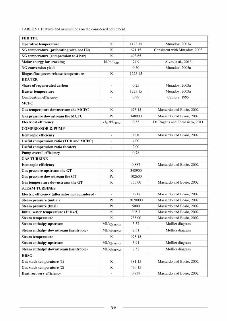
95

TABLE 5.1 Features and assumptions on the considered equipment.

FBR TDC

Operative temperature K 1123.15 Muradov, 2003a

NG temperature (preheating with hot H2) K 671.15 Consistent with Muradov, 2003

NG temperature (compression to 4 bar) K 493.65

Molar energy for cracking kJ/molCH4 74.9 Alves et al., 2013

NG conversion yield - 0.50 Muradov, 2003a

Biogas flue gasses release temperature K 1223.15

HEATER

Share of regenerated carbon - 0.25 Muradov, 2003a

Heater temperature K 1223.15 Muradov, 2003a

Combustion efficiency - 0.99 Cantore, 1995

MCFC

Gas temperature downstream the MCFC K 973.15 Massardo and Bosio, 2002

Gas pressure downstream the MCFC Pa 348900 Massardo and Bosio, 2002

Electrical efficiency kJEL/kJCHEM 0.55 De Rogatis and Fornasiero, 2011

COMPRESSOR & PUMP

Isentropic efficiency - 0.810 Massardo and Bosio, 2002

Useful compression ratio (TCD and MCFC) - 4.00

Useful compression ratio (heater) - 2.00

Pump overall efficiency - 0.78

GAS TURBINE

Isentropic efficiency - 0.887 Massardo and Bosio, 2002

Gas pressure upstream the GT K 348900

Gas pressure downstream the GT Pa 102600

Gas temperature downstream the GT K 755.00 Massardo and Bosio, 2002

STEAM TURBINES

Electric efficiency (alternator not considered) - 0.918 Massardo and Bosio, 2002

Steam pressure (initial) Pa 2070000 Massardo and Bosio, 2002

Steam pressure (final) Pa 5000 Massardo and Bosio, 2002

Initial water temperature (1° level) K 305.7 Massardo and Bosio, 2002

Steam temperature K 735.00 Massardo and Bosio, 2002

Steam enthalpy upstream MJ/kgSTEAM 3.37 Mollier diagram

Steam enthalpy downstream (isentropic) MJ/kgSTEAM 2.31 Mollier diagram

Steam temperature K 973.15

Steam enthalpy upstream MJ/kgSTEAM 3.91 Mollier diagram

Steam enthalpy downstream (isentropic) MJ/kgSTEAM 2.52 Mollier diagram

HRSG

Gas stack temperature (1) K 381.15 Massardo and Bosio, 2002

Gas stack temperature (2) K 470.15

Heat recovery efficiency - 0.839 Massardo and Bosio, 2002

96

TABLE 5.2 Energy balance on the production of biogas/bio-methane from a middle-scale MSW-processing plant.

Parameter Unit of m. Value Reference

Feedstock collection (distance of 12 km) MJ/tDM 540 Pöeschl et al., 2010a

Feedstock transportation (distance of 4 km) MJ/tDM 15.6 Pöeschl et al., 2010a

Feedstock pre-treatment MJel/tDM 216 Pöeschl et al., 2010a

Electricity consumption MJ/MJbiogas 0.039 Börjesson and Ahlgren, 2012

Heat consumption MJ/MJbiogas 0.12 Börjesson and Ahlgren, 2012

Digestate management MJpe/tdigestate 144.55 Pöeschl et al., 2010a

Digestate production tdigestate/tDM 3.3 Pöeschl et al., 2010a

Municipal solid waste solid content tDM/tMSW 0.4 Pöeschl et al., 2010a

Upgrading (membrane) MJ/m3bioCH4 2.00 Molino et al., 2013

Biogas energy content MJ/tDM 6600 Pöeschl et al., 2010a

Biogas yield m3biogas/tDM 308 Pöeschl et al., 2010a

Total production energy consumption MJ/m3bioCH4 18.30

Low heating value MJ/m3bioCH4 32.97 Browne et al., 2011 (modif.)

Net energy available MJ/m3bioCH4 14.67

Molar volume (normal conditions) m3bioCH4/molbioCH

4 0.024

Net molar energy available kJ/molbioCH4 346.8

Total production energy cons. (bioCH4) kJ/molbioCH4 432.8

Total production energy cons. (biogas) kJ/molBIOGAS 231.3

TABLE 5.3 Boundary conditions of the hybrid system and chemical properties of the substances.

Unit CH4 CO2 H2O N2 O2 H2 cp coefficient a J/mol/K 19.89 22.26 32.24 28.9 25.48 29.11

cp coefficient b J/mol/K2 0.05024 0.05981 0.001923 -0.001571 0.0152 -0.001916

cp coefficient c J/mol/K3 12.69 E-06 -35.01 E-06 10.55 E-06 8.081E-06 -7.155 E-06 4.003 E-06

cp coefficient d J/mol/K4 -11 E-09 7.469E-09 -3.595E-09 -2.87E-09 1.312E-09 -8.704E-10

cp (coke) J/mol/K 10.2

Perfect gasses universal constant J/mol/K 8.3145

Environmental temperature K 288.15

Environmental pressure Pa 101325

Alternator efficiency - 0.98 Cantore, 1995

Auxiliary equipment efficiency - 0.95 Cantore, 1995

97

FIGURE 5.2 Hybrid TCD-CCGT system layout.

TABLE 5.4 Plant stream analysis (see FIGURE 5.2 for the different sections): pressure, temperature, specific molar flow and composition.

1 2 3 4 5 6 7 8 9 p (kPa) 101.3 400.0 400.0 ≈ 400.0 ≈ 400.0 ≈ 400.0 ≈ 400.0 ≈ 350.0 ≈ 350.0

T (K) 288.2 493.7 671.2 897.2 1123.2 1123.2 1123.2 973.2 973.2

N (mol/molBG) 5.83 5.83 5.83 11.67 17.5 11.67 5.83 11.67 33.62

Composition NG NG NG NG NG, H2 H2 NG H2 N2, H2O

10 11 12 13 14 15 16 17 18 p (kPa) 102.6 ≈ 101.3 5.0 2070.0 2070.0 101.3 350.0 101.3 ≈ 200.0

T (K) 755.0 381.2 306.0 306.0 735.0 288.2 441.2 1123.2 1123.2

N (mol/molBG) 33.62 33.62 8.34 8.34 8.34 27.79 27.79 5.83 1.46

Composition N2, H2O N2, H2O H2O H2O H2O Air Air C C

19 20 21 22 23 24 25 26 27 p (kPa) ≈ 200.0 101.3 101.3 200.0 ≈ 200.0 101.3 5.0 2070.0 2070.0

T (K) 1223.2 288.2 288.2 363.7 1223.2 470.0 306.0 306.0 973.1

N (mol/molBG) 1.46 1.00 5.71 6.71 6.71 6.71 3.11 3.11 3.11

Composition C Biogas Air Biogas, air

N2, CO2, H2O

N2, CO2, H2O

H2O H2O H2O

98

5.4. ECONOMIC ANALYSIS

This last part strives to complete the former by drawing some financial consideration about the aforesaid technologies. It is important to point up that the available literature data are not specific for the case study totally, because of both the different system layout and the different scale of application. Thus, the attempt to merge and extrapolate such information might end up with approximate conclusions, which can offer some benchmark for more detailed analyses yet.

The economic study is carried out according to as the same scheme as the energy analysis, i.e. a preliminary biogas plant-addressed part followed by a specific technology-addressed counterpart. Once again, one considered the two different biogas-utilisation routes described earlier, both developing from the same middle-scale biogas plant previously hinted. In order to better assess the costs, it is necessary to fix a plant capacity of processed MSW (18000 t/y), which impinges on the overall biofuel production according to the formula:

Plantcapacity × solidcontent × biogasyield = 18000 tãäåy × 0.4 t�ãtãäå × 308mÓÒ�t�ã = 2217600mÓÒ�y

(5.19)

All the accounted for costs are referred to the plant capacity (t or t/y): when no direct data are available, one divided the literature information by the related capacity (Table 5.5). On the other hand, when they are country-specific, they are turned to the Italian standards (e.g. cost of electricity, diesel fuel, see Table 5.6). An important source of earning for the plant is the gate fee on waste which, instead of being paid to the landfill owners, it is intercepted by the plant. Remark: the parameter “Depreciation fund for mechanical and electric equipment” accounts for the element wearing over the depreciation period (10 y), and it is fixed to half the biogas plant capital cost.

TABLE 5.5 Summary of a middle-scale biogas plant costs (the site purchase is not accounted for). Remark: all the costs related to the biogas upgrading are not considered in the second scenario (hybrid power generation system).

Group Parameter Unit of m. Value Reference

Capital costs Biogas plant (dry batch) €/(tMSW/y) 280 Browne et al., 2011

Biogas upgrading plant €/(tMSW/y) 34 Browne et al., 2011

Gas grid connection €/(tMSW/y) 6.0 Browne et al., 2011

Feedstock costs Collection (distance of 12 km) €/tMSW 9.0 Pöeschl et al., 2010a

Transportation (distance of 4 km) €/tMSW 0.3 Pöeschl et al., 2010a

Pre-treatment €/tMSW 22.1 Pöeschl et al., 2010a

Operating costs Maintenance and overheads €/tMSW 25 Browne et al., 2011

Electrical demand of biogas plant €/tMSW 0.9 Browne et al., 2011

Thermal demand of biogas plant €/tMSW 2.0 Browne et al., 2011

Biogas upgrading €/tMSW 10.5 Molino et al., 2013

Digestate disposal €/tMSW 4.0 Browne et al., 2011

Depreciation fund for mechanical and electric equipment

€/tMSW 14.0 Browne et al., 2011

Plant construction period y 1.5 [4]

Incomes Gate fee on waste €/tMSW 70.0 Browne et al., 2011

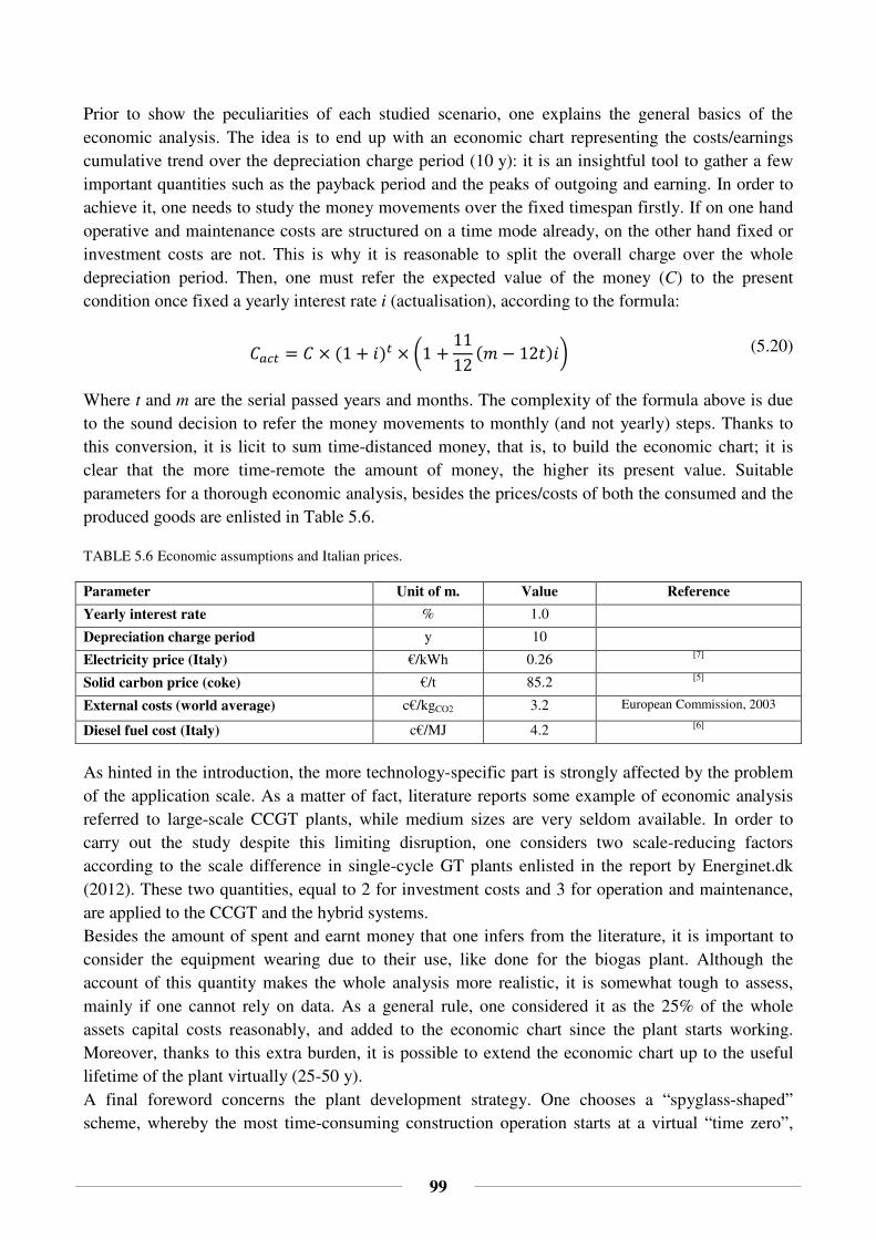
99

Prior to show the peculiarities of each studied scenario, one explains the general basics of the economic analysis. The idea is to end up with an economic chart representing the costs/earnings cumulative trend over the depreciation charge period (10 y): it is an insightful tool to gather a few important quantities such as the payback period and the peaks of outgoing and earning. In order to achieve it, one needs to study the money movements over the fixed timespan firstly. If on one hand operative and maintenance costs are structured on a time mode already, on the other hand fixed or investment costs are not. This is why it is reasonable to split the overall charge over the whole depreciation period. Then, one must refer the expected value of the money (C) to the present condition once fixed a yearly interest rate i (actualisation), according to the formula:

t*¯¥ = t × (1 æ)¥ × 1 1112 (� 12#)æ�

(5.20)

Where t and m are the serial passed years and months. The complexity of the formula above is due to the sound decision to refer the money movements to monthly (and not yearly) steps. Thanks to this conversion, it is licit to sum time-distanced money, that is, to build the economic chart; it is clear that the more time-remote the amount of money, the higher its present value. Suitable parameters for a thorough economic analysis, besides the prices/costs of both the consumed and the produced goods are enlisted in Table 5.6.

TABLE 5.6 Economic assumptions and Italian prices.

Parameter Unit of m. Value Reference

Yearly interest rate % 1.0

Depreciation charge period y 10

Electricity price (Italy) €/kWh 0.26 [7]

Solid carbon price (coke) €/t 85.2 [5]

External costs (world average) c€/kgCO2 3.2 European Commission, 2003

Diesel fuel cost (Italy) c€/MJ 4.2 [6]

As hinted in the introduction, the more technology-specific part is strongly affected by the problem of the application scale. As a matter of fact, literature reports some example of economic analysis referred to large-scale CCGT plants, while medium sizes are very seldom available. In order to carry out the study despite this limiting disruption, one considers two scale-reducing factors according to the scale difference in single-cycle GT plants enlisted in the report by Energinet.dk (2012). These two quantities, equal to 2 for investment costs and 3 for operation and maintenance, are applied to the CCGT and the hybrid systems. Besides the amount of spent and earnt money that one infers from the literature, it is important to consider the equipment wearing due to their use, like done for the biogas plant. Although the account of this quantity makes the whole analysis more realistic, it is somewhat tough to assess, mainly if one cannot rely on data. As a general rule, one considered it as the 25% of the whole assets capital costs reasonably, and added to the economic chart since the plant starts working. Moreover, thanks to this extra burden, it is possible to extend the economic chart up to the useful lifetime of the plant virtually (25-50 y). A final foreword concerns the plant development strategy. One chooses a “spyglass-shaped” scheme, whereby the most time-consuming construction operation starts at a virtual “time zero”,

100

then all the other plants follow it, so that to be finished nearly simultaneously. This is a questionable choice implying high initial investments and a high level of coordination, but given the relatively small scale of the system it might be worth considering that.

The first scenario is the bio-methane-fed CCGT, whose features are summarised in the Table 5.7. The costs of the biogas plant are consistent with the Table 5.5 totally, since the gas turbine works with clean bio-methane only. Similarly, the CCGT plant traces its reference, but in the construction time, where 7 months (0.6 y) is chosen by applying the proportion between large and medium scale in single-cycle GT plants. More detailed information about the costs is reported at the end of the chapter (Table 5.9).

TABLE 5.7 Summary of the bio-methane-fed CCGT power system scenario.

Biogas plant Molar energy available (LHV) MJ/m3bioCH4 33.0

Biogas methane content m3bioCH4/m

3BG 0.60

Biogas flow m3BG/y 2217600

Delivered chemical power GJCHEM/y 43872

Capital costs €/month 48000

Operative and feedstock costs €/month 131759

Gate fee on waste €/month 105000

CCGT plant Electricity efficiency GJEL/GJCHEM 0.60

Delivered electric power kW 834

Construction time y 0.6

Total specific capital costs €/kW 1132

Total specific operative costs €/kW/y 59

Total capital costs €/month 15738

Total operative costs €/month 12343

Total depreciation fund for equipment (25%) €/month 3934

Incomes Total electricity sale €/month 156066

The hybrid power system scenario is more complex than the former obviously, and that makes the assemblage of different items more difficult and uncertain. Yet, the initial biogas plant is the same basically, but all the costs of upgrading are neglected; this assumption is reasonable according to what stated in the previous section, although it is more likely that the raw biogas undergoes some small upgrading. Conversely, the CCGT unit costs are increased with respect to the first scenario lightly, owing to the presence of a second steam turbine. Being data on steam cycles not available directly, one chooses to increase some size-reliant entry of the list of 20%. A final difference concerns the construction time, in this case assumed equal to 2 y, because of the higher amount of produced power (5 MW vs < 1 MW). Data on the TCD unit are retrieved directly from the study of Muradov (2000), where they are likened to the costs of a fluid coking plant. Although the scale of the reference case is very large (production of 106 m3

H2 per day), one does not apply any scale reduction factor, since the most relevant outgoing is represented by the feedstock cost (NG), which is scale-reliant patently. The construction time of a similar FC unit spans from 3 to 5 y, and it is reasonably fixed to 2 y for this medium scale application; therefore, the construction of both the CCGT and the TCD units could

101

start together. The last item of the system is the MCFC, whose assumed costs stem from a trade-off between two references. Energinet.dk (2012) reports investment and operative costs of 5000 €/kW and 25 €/MWh respectively for solid oxide fuel cells (SOFC), while McPhail et al. (2015) states that investment costs for a MCFC are in the range 4000-6000 $/kW. Thus, the chosen values are equal to the first reference, but in US dollars. The construction period is reasonably fixed to 2 months (0.17 y), being the fuel cell a precast item. If on one hand it is worth explaining the higher costs of this second scenario than the first, on the other one expects also higher incomes. They are represented not only by a higher electrical power (5 MW), but also by the sale of solid carbon. Although this is an interesting source of incomes, a more important consideration may be done about its nature. In other words, this combustible and solid carbon stems from natural gas which, with high probability, would have been burnt to water and CO2 otherwise. The already hinted concept of externality (or external cost) should be associated to those anthropic activities giving fossil fuel-derived products off rightly, but it might make sense to consider them within this frame. The assumed carbon cost is estimated according to the price the global warming is given, i.e. 18-46 €/tCO2 (3.2 c€/kgCO2 on average). The following Table 5.8 summarises the costs and the earnings of the hybrid system; once again, more detailed information is given in Table 5.10.

TABLE 5.8 Summary of the biogas-fed hybrid power system scenario.

Biogas plant Biogas flow m3BG/y 2217600

Biogas plant capital costs €/month 42900

Biogas plant operative and feedstock costs €/month 116001

Biogas plant gate fee on waste €/month 105000

TCD unit Delivered hydrogen flow m3H2/y 25869312

Construction time y 2

Total capital costs €/month 10649

Total operative and feedstock costs €/month 352746

MCFC unit Construction time y 0.17

Total investments €/month 192740

Total operative costs €/month 84478

Hybrid plant Net electric energy production MJEL/m3BG 73

Delivered electric power kW 5127

Solid carbon production kg/m3BG 2.96

Avoided CO2 emissions m3NG/m3

BG 5.83

Construction time y 2

Total specific capital costs €/kW 1354

Total specific operative costs €/kW/y 61

Total capital costs €/month 115704

Total operative costs €/month 77980

Total depreciation fund for equipment (25%) €/month 79773

Incomes Total electricity sale €/month 959334

Total carbon sale €/month 46588

Total avoided carbon costs €/month 64186

102

The aim of this economic analysis is the achievement of the economic charts of the two solutions, portrayed in Figure 5.3. Generally, one can claim that the actual and the expected money trends are consistent each other, with an early descending negative phase, corresponding to the construction period, followed by a rising counterpart where the investments are retrieved by means of the incomes. The different slopes that can be gazed in the first phase (much evident in the hybrid system line) are due to the gradual construction beginnings of each component. Although both analyses strove to account for the equipment wearing, the linearly indefinite growth of the earnings is too much unrealistic. One needs to carry out more thorough economic reckonings on such outgoings, besides giving the lines a more meaningful globally swinging trend, being more consistent with the market evolution. This aspect, considered in the biogas plant construction more carefully than elsewhere (because of available references), becomes more and more important the longer the studied timespan and the larger the plant assets. Thus, it is clear that this problem impinges upon the second scenario more than upon the first.

The first scenario (blue line) displays a rather flattened development, with a maximum debt of 1 M€ recorded at the end of the biogas construction (18 months). Then, thanks to the earnings, the system reaches the breakeven point (BEP) after 38 months and then the net income at the end of the decade results 4.4 M€. This solution appears as fruitful and rather safe by a financial standpoint, being the maximum debt relatively low and the payback period short. The second scenario (red line) shows a sharper trend than the former, reaching a maximum debt of 4.24 M€ rapidly at the end of the whole system construction (24 months). Yet, this dramatic early loss is offset by a rise slower than the descent, leading the system to the BEP after 64 months. Approximately 2 y after the BEP achievement, this scenario prevails over the first, enlarging the joint diversion up to a final maximum income of 6.2 M€. It is clear that this is the most fruitful and interesting scenario eventually, in spite of the initial discouraging losses. However, it is necessary to highlight the higher financial uncertainty with respect to the former, due to the fourfold higher debt and the more delayed BEP. These flaws make this solution definitively weaker and more prone to market fluctuations than the previous one. Nonetheless, once identified the start up as the crucial phase of the project, the presence of suitable incentives can favour the overcoming of the early economic effort hopefully. For the sake of presentation, an additional “spinoff” scenario of the hybrid system is considered (green line), being deprived of the carbon externalities. The noteworthy diversion between this scenario and the former is crystal clear, highlighting how much expensive the fossil CO2 emissions are. By extrapolating the line, it is possible to locate the BEP after 129 months (≈ 11 y) and to understand that it will prevail over the CCGT scenario never. Although these two scenarios result highly expensive, it is expedient to point up the large uncertainty impinging on them; a more detailed study, maybe with updated figures, might also reveal lesser outgoings than the modelled one. Moreover, if on one hand the complexity of the system can be regarded to as negative (expensiveness of its parts, market prices fluctuations), on the other hand it is judiciously expected to benefit from the relentless forthcoming technology improvement, increasing the yields and decreasing the prices of its different parts simultaneously.

103

FIGURE 5.3 Economic charts of the three case studies.

Concluding, one may say that the CCGT configuration is the most fruitful scenario, both in terms of electric yield and financial safety. Yet, its carbon neutrality is far less worth than the joint renewability and fossil fuel decarbonisation of the hybrid system. In other words, if on one hand the first solution does not produce any carbon-derived emission, on the other hand the hybrid not only benefits from the carbon sale incomes, but it also reduces the economic drawbacks of fossil fuel emissions thanks to a suitable capture technique. Therefore, it is clear how much profitable the fossil carbon interception is, due to the “twice” nature of the related earnings. However, one may claim that the third scenario represents the real economic chart of the hybrid plant, since the incomes from the CO2 emission saving is virtual only. In order to realise them, one would need to be part of an efficient carbon market, like the emissions trading system (ETS) – endorsed by the Kyoto Protocol – was before the present economic recession. Within this frame, the “red line” would become the real benchmark for the plant, since it encompasses also indirect environmental and social consequences, often neglected, by enlarging the boundaries of the analysis.

TABLE 9 Details of the CCGT plant costs. The adopted currency conversion is 1 £ = 1.4071 €.

Group Parameter Unit of m. Value Reference

Capital costs Pre-licencing costs, technical and design €/kW 18.29 Griffiths, 2011

Regulatory, licencing and public enquiry €/kW 4.08 Griffiths, 2011

Engineering, procurement and construction cost €/kW 1080.65 Griffiths, 2011

Infrastructure cost €/kW 28.99 Griffiths, 2011

Operating costs Operative and maintenance fixed fee €/kW/y 38.38 Griffiths, 2011

Operative and maintenance variable fee €/MWh 0.28 Griffiths, 2011

Insurance €/kW/y 5.76 Griffiths, 2011

Connection and Use of System charges €/kW/y 12.59 Griffiths, 2011

104

TABLE 10 Details of the hybrid plant costs. The adopted currency conversion is 1 $ = 0.9022 €. The star (*) points out those entries increased by the factor 1.2.

Group Parameter Unit of m. Value Reference

Capital costs Reactor, heater and grinder (from FC plant) c€/(m3H2/y) 4.45 Muradov, 2000

Membrane hydrogen separator c€/(m3H2/y) 0.49 Muradov, 2000

Pre-licencing costs, technical and design €/kW 18.29 Griffiths, 2011

Regulatory, licencing and public enquiry €/kW 4.08 Griffiths, 2011

Engineering, procurement and construction cost* €/kW 1296.8 Griffiths, 2011

Infrastructure cost* €/kW 34.78 Griffiths, 2011

MCFC investment €/kW 4510.8 Energinet.dk, 2012; McPhail et al., 2015

Operating costs Feedstock (NG) c€/m3H2 16.02 Muradov, 2000

Catalyst/reagents/desulfurization c€/m3H2 0.25 Muradov, 2000

Power USA electricity price c€/m3H2 0.07 Muradov, 2000

Labour c€/m3H2 0.02 Muradov, 2000

Operative and maintenance fixed fee €/kW/y 38.38 Griffiths, 2011

Operative and maintenance variable fee* €/MWh 0.34 Griffiths, 2011

Insurance* €/kW/y 6.91 Griffiths, 2011

Connection and Use of System charge €/kW/y 12.59 Griffiths, 2011

MCFC operative costs €/MWh 22.6 Energinet.dk, 2012; McPhail et al., 2015

105

6. CONCLUSIONS

In the early chapters, one strove to show the chief biological ways to produce methane and hydrogen, quoting other equally important strategies based on the use of both biomasses and fossil fuels. For sure, the anaerobic digestion showed noteworthy potentialities, among which:

• the “preservation” of the intrinsic chemical energy of the organic substrates, processed by teams of microbes up to the attainment of biogas and bio-hydrogen;

• the consequent sharp decline of greenhouse gasses coming from both the oxidation (composting) and the disposal (landfill gas) of such matter;

• the setup of a virtuous network of people, boards and facilities devoted to an aware and wise management of the natural resources; the production of high-value bio-products (biofuels, bio-fertilisers) able to partially but successfully replace, in the long-term, the fossil and mineral counterparts, with clear environmental benefits (heat and power generation, gas mains injection, vehicle fuels, bio-syngas);

• job opportunities, since the need of trained and entitled staff for the management of the delicate AD stages, as well as the massive employment in the energy crops development.

By a technical standpoint, there is not a best or most fruitful reactor configuration, given the dependence of the type of processed substrate. For a strong and large-scale implementation of AD, feasible in wide urbanised and industrialised areas, high-rate are the most performing digesters, with a continuous feeding (e.g. CSTR) and working under wet conditions. Alternatively, more advanced equipment with attached or suspended biomass (e.g. UASB) offers a higher reliability against the heterogeneity of the substrates. Besides, this availability of plentiful and assorted sources (OFMSW, food process waste, WWTP sludge…) allows the process optimisation by means of a wise co-digestion. Wet but low-rate configurations can successfully serve rural communities, dealing with homogeneous agricultural waste (e.g. fixed-dome plants). On the other hand, the quite simple and cheap batch configurations (e.g. hybrid batch-UASB) proved the best in treating dry matter such as lignocellulose waste and energy crops, thus particularly suitable for small-scale applications like scattered large farms or groups of lesser farms.

The following chapter was focused on the study of the broad and impressive opportunities that bio-methane and bio-hydrogen may have in the forthcoming world’s energetic needs, as well as the difficulties in their application. As a matter of fact, in spite of AD has already become a touchable reality in many Countries (Germany is the leader in Europe), one cannot neglect the paramount endeavours and high financial risks related to its establishment. First of all, the intrinsic complexity and slightness of the process require thorough respect of all the microbial communities, controls over the temperature, the presence of hazardous substances, and the verification of the process stability in the long-term. Secondly, the remarkable initial investments, which might have a

106

somewhat long payback period (3-7 years), so less economically reliable; along with them, the not less important energy inputs (e.g. electricity, heat) and operative costs spread over the lifetime of the plant. It is moreover important to highlight that the costs of production hinge upon the type of processed substrate and the presence of incentives (e.g. gate fee for waste). Browne et al. (2011) report the following VAT-free costs: 1.16 €/m3

bioCH4 for co-digestion of grass and dung, 0.54 for SHW and 0.30 for OFMSW. These strong economic hindrances are detrimental for the “autonomous” implementation of the AD fuels: commingling them with fossil NG (or fossil-derived H2) is the most viable way to enter the market in almost all the utilisation fields nowadays.

Starting from this last remark, one ran energy and economic analyses on two applications associated to the same middle-scale AD plant: a bio-methane-fed CCGT cycle and a biogas-fed hybrid power station, made of a NG-cracking unit, a MCFC and a CCGT cycle. The energetic analysis showed a small difference in the total electric yield between the two cases (0.55 vs 0.52 respectively). However, if the upstream biofuel production chain is considered, the first yield dwindles radically (5%), while the second less (45%), because of the higher electricity yield by the fuel cell. It is reasonable to claim that the hybrid system is more fruitful than the first if the plant “boundaries” are extended to the whole production process. That idea is strengthened in the economic study, where the hybrid can prevail over the CCGT system in a decade-lasting scenario if the environmental benefits from the NG decarbonisation are taken into account. They can be represented by carbon allowances, like the ones suggested by the Kyoto Protocol within the emissions trading system. The absence of such incomes “overturns” the situation completely, highlighting the high economic value of the fossil fuel emissions. Concluding, it is reasonable to claim that, if contextualised suitably, the hybrid scheme does not sanction the failure of the renewables, but in fact it prepares their large-scale access in the energy market. If on one hand the paramount and ground-breaking effort needed to implement the renewables can be agreeably thought as the well-known “chicken or the egg” causality dilemma, on the other hand it can be virtuously worked out through a wisely handled transition period, where all the equipment and the infrastructures are replaced or restyled gradually (and the social acceptance is gained), followed by the simplified – and perhaps definitive – application of the renewables.

107

ADDENDUM: BIOCHEMISTRY RECALLS

In this summarising section, one wants to introduce the basics of organic chemistry which will make the next topics easier to understand. This subject studies the organic compounds that the carbon forms when it is covalently bound to hydrogen, oxygen, nitrogen, phosphorus, sulphur, as well as with up to three covalent bonds with other carbon atoms (an extremely rare property shared with the silicon only). This broad versatility of the carbon atom is chiefly due to the possession of four shareable electrons in the outer shell. Organic compounds like proteins, carbohydrates, nucleic acids and lipids are the essential constituents of every living organism: they are ordinarily assembled by the organisms on their own, although it is possible to get them synthetically. On the contrary, when the bond is ionic (e.g. carbon dioxide and carbonates), the compounds are inorganic. Organic compounds deeply differ from inorganic ones, for instance, being usually burnable, weakly water-soluble, energy sources for many organisms, melting and boiling at lower temperatures. Besides, they can be chemically represented with several formulas: empirical, useful to understand the ratios among the different chemicals (e.g. ethane CH3); molecular, representing the exact quantity of atoms (e.g. C2H6); structural, showing the spatial arrangement of the atoms and the earmarks of the bonds; and semi-structural (or condensed), where the main groups are highlighted (e.g. CH3CH3). Although in many analyses the condensed formula is enough, the structure plays a notable role, since it may change the properties of compounds sharing the same molecular formula; this peculiarity, known as isomerism, affects e.g. the hydrocarbons.

There are many ways to split organic compounds up, but one of the most popular is in aromatic, heterocyclic and aliphatic. The first family display a ring structure with six carbon atoms linked among them with three single and three double bonds. The seconds are ring-shaped too, but with one carbon atom replaced by another chemical, usually nitrogen, oxygen and sulphur. Aliphatic compounds are linear, branched or cyclic frames of C atoms joined with single bonds only, thus called saturated; as they are the most studied in the continuation, a more detailed description of the different groups is reported. Alkanes (or paraffins) are the simplest hydrocarbons, with C atoms both joined among them and with hydrogen atoms (Table A.1). They are summarised with the general formula CnH2(n+1), which patently shows that the main distinction among them is the number of C atoms. Alkanes are rather stable odourless and colourless compounds, soluble in organic solvents, but not in water. The removal of a H atom from the chain gives rise to a very reactive radical alkyl group (e.g. methyl, ethyl...). The chain of the linear alkanes grows by adding a methylene group (CH2) and the different compounds thus produced are said to form a homologous series. Actually, there are other more complicated configurations, like the branched alkanes, where H atoms are replaced by methyl groups, or the cycloalkanes, where the linear chain is closed by replacing the two external H atoms with a C–C bond. The functional group C–C is more robust than

108

the C–H bond, but both can be thermally broken into shorter compounds: the process, named cracking, is widely applied to long-chain alkanes.

TABLE A.1 Physical properties of the first ten alkanes.

Name Formula Melting point (K) Boiling point (K) Density at 293.1 K (kg/m3) LHV (MJ/kg) Methane CH4 90.6 111.4 555 (at 273.1 K) 50.01 Ethane C2H6 89.8 184.5 509 (at 213.1 K) 47.80 Propane C3H8 85.4 231.0 500 46.36 Butane C4H10 134.8 272.6 579 45.75 Pentane C5H12 143.3 309.2 557 45.36 Hexane C6H14 177.8 341.8 660 44.75 Heptane C7H16 182.5 371.5 684 44.57 Octane C8H18 216.3 398.8 703 44.43 Nonane C9H20 219.6 423.9 718 44.31 Decane C10H22 243.4 447.1 730 44.24

Similar to alkanes, there are the unsaturated alkenes or olefins (CnH2n) and the alkynes (CnH2(n-1)), respectively characterised by one double and one triple bond between two C atoms. They are not approached in the follow-up, but it is noteworthy to quote that alkenes burn with O2 like the alkanes and that, under particular thermodynamic conditions (high p and T) and thanks to a catalyst, they undergo a polymerisation process, whereby they combine each other bringing about widely used polymers, like polyethene and polyvinyl chloride (PVC). Alcohols are derivatives of alkanes, usually after a partial biological oxidation (formula A.1). The structure is quite similar, with only a H atom replaced with a hydroxyl group (-OH); therefore, the generic molecular formula is CnH(2n+1)OH, despite they are commonly represented as R-OH, where R stands for the alkyl group. Alcohols are usually numerated according to the position of the C atom which the -OH group is stuck to; similarly, the presence of one, two and three R groups attached to the first carbon distinguishes primary, secondary and tertiary alcohols, which may be branched methylated versions too. The presence of the hydroxyl group makes the alcohols more reactive than alkanes, and that is the reason why they are water-soluble and many H bonds form among alcohol molecules. Although the weakness of those bonds, the huge amount of them gives an overall effect of robustness, so much so that they have higher boiling temperatures than alkanes. Alcohols are well-known for their high volatility and flammability, which allows them to be used as biofuels (e.g. bioethanol and bio-butanol instead of petrol): the reaction is an exothermic oxidation (formula A.2). Yet, they may even undergo reversible oxidation processes whereby aldehydes and ketones are brought about, respectively from primary and secondary alcohols.

2CYH�(Y_;) + O� DYçXZDEFFFFG 2CYH(�Y_;)OH (A.1)

2CYH(�Y_;)OH + 3nO� → 2nCO� + 2(n + 1)H�O + ∆H�R (A.2)

Carboxylic acids are aliphatic compounds stemming from the oxidation of primary alcohols, aldehydes or alkanes, where in his case the methyl group -CH3 is replaced by a carboxylic one -COOH: thus, the general formula is R-COOH. Again, carboxylic acids can be liable to replacements of H with other atoms according to the aforesaid mechanisms. They play a remarkable role in many biologic systems, since many microorganisms consume them as energy sources, with an oxidation process. Like alcohols, their ability to form H bonds raises their melting and boiling points, as well as their water-solubility: anyhow, this last aspect gradually diminishes with the rise

109

of the chain of carbon atoms and its hydrophobia. As a matter of fact, hexanoic acid almost no more soluble and since the nonanoic acid, they take a greasy aspect at room temperature. As it may be easily inferred from the low solubility, those acids are weak, and that is confirmed by the logarithm of the acid dissociation constant pKa, which is always greater than -2. Hence, it is clear that the properties of those compound are sharply affected by the length of the chain, and it is particularly evident concerning the well-known fatty acids, which are the building blocks of fats: short-chain SCFA (or volatile VFA < 6 carbons), medium-chain MCFA (6-12 carbons) and long-chain fatty acids LCFA (> 12 carbons). In carboxylic acids, it is particularly important to compare the IUPAC name with the common one, since the last one points out the first substrate which the acid was isolated from the first time (Table A.2). That is easily understandable when one consider their peculiar smell, which moves from the acid everyone is familiar with (ethanoic acid) to the disgusting one of rancid milk-derivatives (butanoic acid).

TABLE A.2 Physical properties of the first ten organic acids. The star (*) refers to a temperature of 293.1 K.

IUPAC name Common name Formula TMELTING (K) TBOILING (K) Density* (kg/m3)

Methanoic acid Formic acid HCOOH 281.5 373.8 1220.0

Ethanoic acid Acetic acid CH3COOH 289.7 391.0 1042.2

Propanoic acid Propionic acid CH3CH2COOH 252.3 414.1 993.0

Butanoic acid Butyric acid CH3(CH2)2COOH 268.8 436.6 957.7

Pentanoic acid Valeric acid CH3(CH2)3COOH 239.3 459.2 939.1

Hexanoic acid Caproic acid CH3(CH2)4COOH 271.1 478.1 927.4

Heptanoic acid Enanthic acid CH3(CH2)5COOH 265.6 496.1 920.0

Octanoic acid Caprylic acid CH3(CH2)6COOH 289.6 512.4 908.8

Nonanoic acid Pelargonic acid CH3(CH2)7COOH 285.3 528.1 905.7

Decanoic acid Capric acid CH3(CH2)8COOH 304.6 543.1 885.8

The last family of organic compounds presented in this recall are nitrogen-containing organic compounds (Figure A.1). Amines (primary, secondary or tertiary) stem from ammonia (NH3), wherein one, two or three H molecules were replaced by a generic organic group R. When R is embodied by an alkyl group, they are referred to as alkanamines. They are the most important nitrogen sources in many biologic systems, as well as the building blocks of amino acids and, then, proteins. Conversely, amides are derivatives of carboxylic acids, characterised by the replacement of the hydroxyl group with –NH2. The remaining hydrogen atoms can be even replaced like in the amines, giving rise to the secondary and the tertiary structures.

Figure A.1 Several types of amines (left) and amides (right).

110

REFERENCES

ABÁNADES A., RUIZ E., FERRUELO E. M., HERNÁNDEZ F., CABANILLAS A., MARTÍNEZ-VAL J. M., RUBIO J. A., LÓPEZ C., GAVELA R., BARRERA G., RUBBIA C., SALMIERI D., RODILLA E., GUTIÉRREZ D.,

2011. Experimental analysis of direct thermal methane cracking. International Journal of Hydrogen Energy 36, 12877 – 12886.

ABBASI T., TAUSEEF S. M., ABBASI S. A., 2012. Biogas Energy. Springer-Engineering, New York.

AL SEADI T., 2002. Quality management of AD residues from biogas production. IEA Bioenergy, Task

24 – Energy from Biological Conversion of Organic Waste.

AL SEADI T., RUTZ D., PRASSL H., KÖTTNER M., FINSTERWALDER T., VOLK S., JANSSEN R., 2008. Biogas Handbook. Ed. T. A. Seadi. University of Southern Denmark Esbjerg, Niels Bohrs.

ALVES H. J., BLEY C. JR., NIKLEVICZ R. R., PIRES FRIGO E., SATO FRIGO M., COIMBRA-ARAÙJO C. H., 2013.

Overview of hydrogen production technologies from biogas and the applications in fuel cells. International journal of hydrogen energy 38, 5215-5225.

ANGELINO G., GAIA M., MACCHI E., 1984. A review of Italian activity in the field of Organic Rankine Cycles. Proceedings of the International VDI-Seminar held in Zürich.

APPELS L., LAUWERS J., DEGRÈVE J., HELSEN L., LIEVENS B., WILLEMS K., VAN IMPE J., DEWIL R., 2011.

Anaerobic digestion in global bio-energy production: Potential and research challenges. Renewable

and Sustainable Energy Reviews 15, 4295-4301.

ARSOVA L., THEMELIS N. J., CHANDRAN K., 2010. Anaerobic digestion of food waste: Current status, problems and an alternative product, M.S. Degree in Earth Resources Engineering, New York.

ASSABUMRUNGRAT S., PHROMPRASIT J., BOONKRUE S., KIATKITTIPONG W., WIYARATN W., SOOTTITANTAWAT

A., ARPORNWICHANOP A., LAOSIRIPOJANA N., POWEL J., 2012. Energy Efficiency Evaluation for a ‘‘Green’’ Power Generation Process with Minimum Effort on Carbon Dioxide Capture and Storage. Chemical Engineering Communications 199, 1642-1651.

BASERGA U., 1998. Landwirtschaftliche Co-vergarungs-Biogasanlagen, FAT-Berichte No. 512, Tanikon.

BAROMÈTRE BIOGAZ, EUROBSERV’ER, 2012. Systèmes solaires. Le journal des énergies renouvelables n°212.

BHATTACHARYA A., DAS A., DATTA A., 2014. Exergy based performance analysis of hydrogen production from rice straw using oxygen blown gasification. Energy 69, 525-533.

111

BIEŃ J. B., MILCZAREK M., NECZAJ E., GAŁWA-WIDERA M., 2010. Co-composting of industrial sewage sludge from mineral water production plant “Jurajska” in Postep and municipal sewage sludge. Polish Journal of Environmental Studies 2, 7-11.

BIOENERGY IEA, 2009. Biogas upgrading technologies - developments and innovations. Available from: www.iea-biogas.net.

BOCKRIS J. O’ M., 2002. The origin of ideas on a Hydrogen Economy and its solution to the decay of the environment. International Journal of Hydrogen Energy 27, 731-740.

BORDELANNE O., MONTERO M., BRAVIN F., PRIEUR-VERNAT A., OLIVETI-SELMI O., PIERRE H., PAPADOPOULO M.,

MULLER T., 2011. Biomethane CNG hybrid: A reduction by more than 80% of the greenhouse gases emissions compared to gasoline. Journal of Natural Gas Science and Engineering 3, 617-624.

BÖRJESSON M., AHLGREN E. O., 2012. Cost-effective biogas utilisation - A modelling assessment of gas infrastructural options in a regional energy system. Energy 48, 212-226.

BOZANO GANDOLFI P., WILJAN H., 1999. Digestione anaerobica di biomasse da rifiuti solidi urbani, industriali e liquami zootecnici con la tecnologia BTA.

BROWNE J., NIZAMI A.-S., THAMSIRIROJ T., MURPHY J. D., 2011. Assessing the cost of biofuel production with increasing penetration of the transport fuel market: A case study of gaseous biomethane in Ireland. Renewable and Sustainable Energy Reviews 15, 4537-4547.

CALLAGHAN F. J., WASE D. A. J., THAYANITHY K., FORSTER C. F., 2002. Continuous co-digestion of cattle slurry with fruit and vegetable wastes and chicken manure. Biomass and Bioenergy 27, 71-77.

CANTORE G., 1995. Macchine. Appunti tratti dalle lezioni del Prof. Giuseppe Cantore. Terza edizione. Società editrice Esculapio, Bologna.

CECCHI F., BATTISTONI P., PAVAN P., BOLZONELLA D., INNOCENTI L., 2005. Digestione anaerobica della frazione organica dei rifiuti solidi. Manuali e linee guida. APAT.

CHANG A. C.-C., CHANG H.-F., LIN K.-H., LIN W.-H., CHEN S.-H., CHANG C.-Y., 2013. Autothermal steam reforming of glycerol for hydrogen production over packed-bed and Pd/Ag alloy membrane reactors. International journal of hydrogen energy 38, 12946-12952.

CHAUDHARI A.B, SURYAWANSHI P.C, KOTHARI R.M, 2012. Microbial Aspects of Anaerobic Digestion for Biogas Production. In: Anaerobic Digestions. Nova Science Publishers, Inc., 149-174.

CHENG S., LIU W., 2014. Microbial Fuel Cells and Other Bio-Electrochemical Conversion Devices. Electrochemically Enabled Sustainability, CRC Press, 80-91.

CHERUBINI F., 2010. The biorefinery concept: Using biomass instead of oil for producing energy and chemicals. Energy Conversion and Management 51, 1412-1421.

CROISET E., AMIN A. M., EPLING W., 2011. Review of methane catalytic cracking for hydrogen production. International Journal of Hydrogen Energy 36, 2904 – 2935.

112

DATTA A., BHATTACHARYA AT., BHATTACHARYA AB., 2012. Modeling of hydrogen production process from biomass using oxygen blown gasification. International journal of hydrogen energy 37, 18782-18790.

DAS D., KHANNA N., DASGUPTA C. N., 2014. Biohydrogen Production: Fundamentals and Technology Advances. CRC Press, 37-76.

DAMEN K., FAAIJ A., TURKENBURG W., 2006. Health, Safety and Environmental Risks of Underground CO2 Storage Overview of Mechanisms and Current Knowledge. Climatic Change V74(1), 289-318.

DAVIS M., CORNWELL D., 1998. Introduction to Environmental Engineering. WCB/McGraw-Hill, New York.

DEL BORGHI A., CONVERTI A., PALAZZI E., DEL BORGHI M., 1999. Hydrolysis and thermophilic anaerobic digestion of sewage sludge and organic fraction of municipal solid waste. Bioprocess Engineering 20, 553-560.

DE ROGATIS L., FORNASIERO P., 2011. Future Perspectives for Hydrogen as Fuel in Transportation. Renewable Resources and Renewable Energy: A Global Challenge. Taylor & Francis Group LLC, 243-288.

EASTMAN J. A., FERGUSON J. F., 1981. Solubilization of particulate organic carbon during the acid phase of anaerobic digestion. Journal Water Pollution Control Federation 53(3), 352-366.

ECKERMANN E., 2001. World History of the Automobile. Society of Automotive Engineers.

ENERGINET.DK, ENERGI SYRELSEN, 2012. Technology Data for Energy Plants. Generation of Electricity and District Heating, Energy Storage and Energy Carrier Generation and Conversion. ISBNwww: 978-87-7844-931-3.

ENVITECH BIOGAS, 2006. The World’s Largest Biogas Park in Pekun, EnviTec Biogas, Ed. NAWARO BioEnergie AG, Lohne, Germany.

ERKUT E., KARAGIANNIDIS A., PERKOULIDIS G., TJANDRA S. A., 2008. A Multi-Criteria Facility Location Model for Municipal Solid Waste Management in North Greece. European Journal of Operational Research 187, 1402-1421.

ESCAMILLA-ALVARADO C., VAZQUEZ-BARRAGAN J. A., PONCE-NOYOLA M. T. ET AL., 2011. A novel biorefinery approach for biofuels and holocelullolytic enzymes production from organic wastes. In: Bioremediation and Sustainable Environmental Technologies-2011. Battelle first international symposium on bioremediation and sustainable environmental technologies (eds Wickramanayake GB and Rectanus H) Reno, NV, USA. Battelle, Columbus, OH, USA.

EUROPEAN COMMISSION, 2003. External Costs. Research results on socio-environmental damages due to electricity and transport.

EVANS A., STREZOV V., EVANS T. J., 2015. Anaerobic Digestion. In: Biomass Processing Technologies. CRC Press. 177-212.

113

GALVAGNO A., CHIODO V., URBANI F., FRENI F., 2013. Biogas as hydrogen source for fuel cell applications. International journal of hydrogen energy 38, 3913-3920.

GHOSH S., JOY S., DAS D., 2010. Multiple parameters optimization for maximization of hydrogen production using defined microbial consortia. Indian Journal of Biotechnology 10, 196-201.

GIBBINS J., CHALMERS H., 2008. Carbon capture and storage. Energy Policy 36, 4317-4322.

GRIFFITHS B., 2011. Electricity Generation Cost Model - 2011 Update Revision 1.Department for Energy and Climate Change.

GROSSER A., WORWĄG M., NECZAJ E., KAMIZELA T., 2013. Co-digestion of Organic Fraction of Municipal Solid Waste with different organic wastes: A review. Environmental Engineering IV - Pawłowski, Dudzińska & Pawłowski (eds). Taylor & Francis Group, London.

HAKALEHTO E., JÄÄSKELÄINEN A., HUMPPI T., HEITTO L., 2012. Biorefineries using waste – production of energy and chemicals from biomasses by micro-organisms. In: Biomass as Energy Source. Resources, Systems and Applications. CRC Press.

HAWKES F. R., FORSEY H., PREMIER G. C., DINSDALE R. M., HAWKES D. L., GUWY A. J., MADDY J., CHERRYMAN S.,

SHINE J., AUTY D., 2008. Fermentative production of hydrogen from wheat flour industry co-product. Bioresource Technology 99, 5020-5029.

HIRSCH D., EPSTEIN M., STEINFELD A., 2001. The solar thermal decarbonization of natural gas. International Journal of Hydrogen Energy 26, 1023–1033

HOLM-NIELSEN J. B., AL SEADI T., OLESKOWICZ-POPIEL P., 2009. The future of anaerobic digestion and biogas utilization. Bioresource Technology 100, 5478-5484.

HSU C.-W., CHANG P.-L., HSIUNG C.-M., LIN C.-Y., 2013. Constructing an innovative Bio-Hydrogen. Integrated Renewable Energy System. International journal of hydrogen energy 38, 15660-15669.

HUANG S.-T., CHANG A. C.-C., 2013. Multivariate statistics to evaluate factors affecting hydrogen production in a pilot-scale operation system. International journal of hydrogen energy 38, 15843-15848.

INYANG M., GAO B., PULLAMMANAPPALLIL P., DING W., ZIMMERMAN A. R., 2010. Biochar from anaerobically digested sugarcane bagasse. Bioresource Technology 101, 8868-8872.

INYANG M., GAO B., YAO Y., XUE Y., ZIMMERMAN A. R., PULLAMMANAPPALLIL P., CAO X., 2012. Removal of heavy metals from aqueous solution by biochars derived from anaerobically digested biomass. Bioresource Technology 110, 50-56.

JIANG X., SOMMER S. G., CHRISTENSEN K. V., 2011. A review of the biogas industry in China. Energy Policy 39, 6073-6081.

114

JURY C., BENETTO E., KOSTER D., SCHMITT B., WELFRING J., 2010. Life Cycle Assessment of biogas production by monofermentation of energy crops and injection into the natural gas grid. Biomass and bioenergy 34, 54-66.

KALTSCHMITT M., HARTMANN H., HOFBAUER H., EDITORS, 2009. Energie aus Biomasse: Grundlagen, Techniken und Verfahren (2nd edition). Dordrecht, Heidelberg, London, New York: Springer, ISBN 9783540850946.

KANG D. W., KIM T. S., HUR K. W., PARK J. K., 2012. The effect of firing biogas on the performance and operating characteristics of simple and recuperative cycle gas turbine combined heat and power systems. Applied Energy 93, 215-228.

KYMÄLÄINEN M., LÄHDE K., ARNOLD M., KUROLA J. M., ROMANTSCHUK M., KAUTOLA H., 2012. Biogasification of biowaste and sewage sludge e Measurement of biogas quality. Journal of Environmental Management 95, S122-S127.

LACOURA S., CHINESEA T., ALKADEEB D., PERILHONB C., DESCOMBES G., 2012. Energy and environmental balance of biogas for dual-fuel mobile applications. Renewable and Sustainable Energy Reviews 16, 1745-1753.

LI Y., PARK S. Y., ZHU J., 2011. Solid-state anaerobic digestion for methane production from organic waste. Renewable and Sustainable Energy Reviews 15, 821-826.

LINGAIAH V., RAJASEKARAN P., 1986. Biodigestion of cow dung and organic wastes mixed with oil cake in relation to energy. Agricultural Wastes 17, 161-173.

MASSARDO A. F., BOSIO B., 2002. Assessment of Molten Carbonate Fuel Cell models and integration with Gas and Steam Cycles. Journal of Engineering for Gas Turbines and Power, Vol. 124, 103 – 109.

MENZI H., 2002. Manure management in Europe: results of a recent survey. In: Proceedings of the 10th Conference of the FAO/ESCORENA Network on Recycling Agricultural, Municipal and Industrial Residues in Agriculture (RAMIRAN), 14-18 May, Strbske Pleso, Slovak Republic, 93-102.

MCPHAIL S. J., LETO L., DELLA PIETRA M., CIGOLOTTI V., MORENO A., 2015. International status of molten carbonate fuel cells technology (dossier). Advanced Fuel Cells Implementing Agreement, Annex 23 – MCFC.

MILLET P., 2006. GenHyPEM: an EC-supported STREP program on high pressure PEM water electrolysis. World Hydrogen Energy Conference, Lyon France.

MOLINO A., MIGLIORI M., DING Y., BIKSON B., GIORDANO G., BRACCIO G., 2013. Biogas upgrading via membrane process: Modelling of pilot plant scale and the end uses for the grid injection. Fuel 107, 585-592.

MØLLER J., BOLDRIN A., CHRISTENSEN T., 2009. Anaerobic digestion and digestate use: accounting of greenhouse gases and global warming contributions. Waste Management & Research 27, 813-824.

115

MONNET F., 2003. An Introduction to Anaerobic Digestion of Organic Wastes. Final Report. Remade Scotland.

MORINI M., CADORIN M., PINELLI M., 2010. Numerical analyses of high Reynolds number flow of high pressure fuel gas through rough pipes. International journal of hydrogen energy 35, 7568-7579.

MURADOV N., 2000. Thermocatalytic CO2-free production of hydrogen from hydrocarbon fuels. Proceedings of the 2000 Hydrogen Program Review, NREL/CP-570-28890.

MURADOV N., 2003a. Thermocatalytic process for CO2-free production of hydrogen and carbon from hydrocarbons. United States Patent n°US006670058B2.

MURADOV N. Z., 2003b. On-site production of hydrogen from hydrocarbon fuels with minimal greenhouse gas emissions. Fuel Chemistry Division Preprints 48(1), 332.

NATH K., KUMAR A., DAS D., 2006. Effect of some environmental parameters on fermentative hydrogen production by Enterobacter cloacae DM11. Canadian Journal of Microbiology Research 532, 525-532.

NATH K., DAS D., 2008. Effect of light intensity and initial pH during hydrogen production by an integrated dark and photofermentation process. International Journal of Hydrogen Energy 34, 7497-7501.

NAYONO S. E., 2009. Anaerobic digestion of organic solid waste for energy production. Karlsruhe KIT Scientific Publication

NAJA G. M., ALARY R., BAJEAT P., BELLENFANT G., GODON J.-J., JAEG J.-P., KECK G., LATTES A., LEROUX C., MODELON H., MOLETTA-DENAT M., RAMALHO J O., ROUSSELLE C., WENISCH S., ZDANEVITCH I., 2011.

Assessment of biogas potential hazards. Renewable Energy 36, 3445-3451.

NIELSEN H., UELLENDAHL H., AHRING B., 2007. Regulation and optimization of biogas process: Propionate as a key factor. Biomass & Bioenergy 31, 820-830.

NIZAMI A.-S, 2012. Anaerobic Digestion: Processes, Products and Applications. In: Anaerobic Digestions. Nova Science Publishers, Inc., 133-147.

ORECCHINI F., BOCCI E., 2007. Biomass to hydrogen for the realization of closed cycles of energy resources. Energy 32, 1006-1011.

OSTREM K., THEMELIS N. J., 2004. Greening Waste: Anaerobic Digestion for Treating the Organic Fraction of Municipal Solid Wastes. Columbia University, New York, p. 59.

PAN C. M., FAN Y. T., XING Y., HOU H. W., ZHANG M. L., 2008. Statistical optimization of process parameters on biohydrogen production from glucose by Clostridium sp. Fanp2. Bioresource Technology 99, 3146-3154.

PATTERSON T., ESTEVES S., DINSDALE R., GUWY A., 2011. Life cycle assessment of biogas infrastructure options on a regional scale. Bioresource Technology 102, 7313-7323.

116

PATTERSON T., ESTEVES S., DINSDALE R., GUWY A., MADDY J., 2013. Life cycle assessment of biohydrogen and biomethane production and utilisation as a vehicle fuel. Bioresource Technology 131, 235-245.

PERSSON M., 2003. Evaluation of upgrading techniques for biogas [Internet] Lund. School of Environmental Engineering. Available from http://www.sgc.se/dokument/Evaluation.pdf.

PINTAR A., DJINOVIĆ P., ERJAVEC B., GASAN OSOJNIK ČRNIVEC I., 2013. Catalytic Reforming of Biogas into Syngas Using Supported Noble-Metal and Transition-Metal Catalysts . Producing Fuels and Fine Chemicals from Biomass Using Nanomaterials, CRC Press, 121-136.

POGGI-VARALDO H. M., MUNOZ-PAEZ K. M., ESCAMILLA-ALVARADO C., ROBLEDO-NARVÁEZ P. N., PONCE-NOYOLA M. T., CALVA-CALVA G., RÍOS-LEAL E., GALÍNDEZ-MAYER J., ESTRADA-VÁZQUEZ C., ORTEGA-

CLEMENTE A., RINDERKNECHT-SEIJAS N. F., 2014. Biohydrogen, biomethane and bioelectricity as crucial components of biorefinery of organic wastes: A review. Waste Management & Research 32(5), 353-365.

PÖESCHL M., WARD S., OWENDE P., 2010a. Evaluation of energy efficiency of various biogas production and utilization pathways. Applied Energy 87, 3305-3321.

PÖESCHL M., WARD S., OWENDE P., 2010b. Prospects for expanded utilization of biogas in Germany. Renewable and Sustainable Energy Reviews 14, 1782-1797.

RUTLEDGE B., 2005. California biogas industry assessment white paper. Pasadena, USA: WestStart-Calstart; p. Report.

RYCKEBOSCH E., DROUILLON M., VERVAEREN H., 2011. Techniques for transformation of biogas to biomethane. Biomass and bioenergy 35, 1633-1645.

SANDER K., MURTHY G. S., 2010. Life cycle analysis of algae biodiesel. International journal of Life Cycle Assessment, 15704-15714.

SASSE L., 1984. Biogas plants: design and detail of simple biogas plants. Vieweg.

SAXENA R. C., SEAL D., KUMAR S., GOYAL H. B., 2008. Thermo-chemical routes for hydrogen rich gas from biomass: a review. Renewable & Sustainable Energy Reviews 12, 1909-1927.

SCHOENUNG J. M., YU M., MUY S., QUADER F., BONIFACIO A., VARGHESE R., CLERIGO E., BIERY M., MEI M.,

CUTLER D., 2013. Combined Hydrogen, Heat and Power (CHHP) pilot plant design. International journal of hydrogen energy 38, 4881-4888.

SCHANBACHER F., 2009. Anaerobic Digestion: Overview & Opportunities. Ohio State University, Wooster, OH.

SCHRÖDER C., SELIG M., SCHÖNHEIT P., 1994. Glucose fermentation to acetate, CO2 and H2 in the anaerobic hyperthermophilic eubacterium Thermotoga maritima: Involvement of the Embden-Meyerhof pathway. Archives of Microbiology, 161(6), 460-470.

SHAH Y. T., 2014. Anaerobic Digestion of Aqueous Waste for Methane and Hydrogen. In: Water for Energy and Fuel Production. CRC Press, 205-232.

117

STEINBERG M., 1999. Fossil fuel decarbonization technology for mitigating global warming. International Journal of Hydrogen Energy 13, 771-777.

STEINFELD H., GERBER P., WASENAAR T., CASTEL V., ROSALES M., DE HAAN C., 2006. Livestock’s long shadow. Environmental Issues and Options. Food and Agriculture Organisation (FAO) of United Nations.

STREVETT K. A., VIETH R. F., GRASSO D., 2005. Chemo-autotrophic biogas purification for methane enrichment: mechanism and kinetics. Chemical Engineering Journal and the Biochemical Engineering Journal 58, 71-79.

SUBRAMANIAN K. A., MATHAD V. C., VIJAY V. K., SUBBARAO P. M. V., 2013. Comparative evaluation of emission and fuel economy of an automotive spark ignition vehicle fuelled with methane enriched biogas and CNG using chassis dynamometer. Applied Energy 105, 17-29.

SZARKA N., SCHOLWIN F., TROMMLER M., FABIAN JACOBI H., EICHHORN M., ORTWEIN A., THRÄN D., 2013. A novel role for bioenergy: A flexible, demand-oriented power supply. Energy 61, 18-26.

THAMSIRIROJ T., SMYTH H., MURPHY J. D., 2011. A roadmap for the introduction of gaseous transport fuel: A case study for renewable natural gas in Ireland. Renewable and Sustainable Energy Reviews 15, 4642-4651.

TRELOAR R. D., 2010. Gas Installation Technology. 2nd edition. John Wiley & Sons.

UNdata, Energy statistics database. United Nations Statistical Division, 2012.

U.S. DEPARTMENT OF ENERGY, 2010. http://www.netl.doe.gov/research/coal/energy-systems/gasification/gasification-plant-databases/current-world-region

UUSITALO V., SOUKKA R., HORTTANAINEN M., NISKANEN A., HAVUKAINEN J., 2013. Economics and greenhouse gas balance of biogas use systems in the Finnish transportation sector. Renewable Energy 51, 132-140.

VINNERAS B., SCHONNING C., NORDIN A., 2006. Identification of the microbiological community in biogas systems and evaluation of microbial risks from gas usage. Science of the Total Environment 367, 606-615.

WEILAND, P., 2005. Results and Bottle Necks of Energy Crop Digestion Plants-Required Process Technology Innovations, Workshop: Energy Crops and Biogas, Ed. Federal Agricultural Research Centre (FAL). Utrecht, The Netherlands.

WEILAND P., 2010. Biogas production: Current state and perspectives. In: Applied Microbiology and Biotechnology 85, 849-860.

WINSLEY P., 2007. Biochar and bioenergy production for climate change mitigation. New Zealand Science Review Vol. 64 (1), 5-10.

118

WINTER C.-J., 2011. Hydrogen Energy-Abundant, Efficient, Clean: A Debate over the Energy-System-of-Change. In: Carbon-Neutral Fuels and Energy Carriers. CRC Press, 115-130.

YEH S., 2007. An empirical analysis on the adoption of alternative fuel vehicles: the case of natural gas vehicles. Energy Policy 35, 5865-5875.

ZAHER U., CHEONG D., WU B., CHEN S., 2007. Producing Energy and Fertilizer From Organic Municipal Solid Waste. Department of Biological Systems Engineering, Washington State University. Ecology Publication No. 07-07-024.

ZGLOBISZ N., CASTILLO-CASTILLO A., GRIMES S., JONES P., 2010. Influence of UK energy policy on the deployment of anaerobic digestion. Energy Policy 38, 5988-5999.

ZHENG M., TAKEI K., HSIA B., FANG H., ZHANG B., FERRALIS N., KO H., CHUEH Y.-L., ZHANG Y., MABOUDIAN R.,

JAVEY A., 2010. Metal-catalyzed crystallization of amorphous carbon to graphene. Applied Physics Letters 96, 063110.

ZHU L. D., HILTUNEN E., ANTILA E., ZHONG J. J.,.YUAN Z. H., WANG Z. M., 2014. Microalgal biofuels: Flexible bioenergies for sustainable development. Renewable and Sustainable Energy Reviews 30, 1035-1046.

WEB REFERENCES

[1] http://www.ogniwa-paliwowe.info/mcfc.php

[2] http://www.iea.org/publications/freepublications/publication/CCS_roadmap_foldout.pdf

[3] http://www.epa.gov/climatechange/ghgemissions/global.html

[4] http://www.aat-biogas.at/en/news/news-detail/article/villa-di-tirano-it/

[5] http://www.steelonthenet.com/files/metallurgical-coal.html

[6] http://autotraveler.ru/en/spravka/fuel-price-in-europe.html#.VZ-dWyww-P8

[7] https://www.energy.eu/#domestic