Embed Size (px)
Citation preview
Economic Modelling 43 (2014) 305–320
Contents lists available at ScienceDirect
Economic Modelling
j ourna l homepage: www.e lsev ie r .com/ locate /ecmod
Allocative inefficiency and sectoral allocation of labor: Evidence fromU.S. agriculture☆
Talan B. İşcan ⁎Department of Economics, Dalhousie University, 6214 University Avenue, Halifax, P.O. Box 15000, NS, B3H 4R2, Canada
☆ I thank an anonymous reviewer, Andrea Giusto, DozOsberg, Richard Rogerson, and Kuan Xu for detailed coShimmin at NASS for data and answering my questions abDíaz-Insensé for editorial suggestions. This research wasthe author declares no competing financial interest.⁎ Tel.: +1 902 494 6994.
E-mail address: [email protected]: http://myweb.dal.ca/tiscan/.
1 In particular, there is a growing literature on allocativefrom U.S. manufacturing industries. See, for instance, Olleyand Doms (2000), Foster et al. (2008), Petrin et al. (2011),Hsieh and Klenow (2009) for a study of inefficient amanufacturing plants in China and India relative to that in
http://dx.doi.org/10.1016/j.econmod.2014.08.0060264-9993/© 2014 Elsevier B.V. All rights reserved.
a b s t r a c t
a r t i c l e i n f oArticle history:Accepted 22 August 2014Available online xxxx
Keywords:Inefficient allocation of resourcesReallocation of laborAgricultureFactor-augmenting technologyUnited States
Are productivity differences across producers in an industry a good indicator of allocative inefficiency? If so,whatare the welfare consequences of reallocating labor from lesser to more productive producers? This paperaddresses these questions in the context of factor specificity, which generates endogenous distribution of totalfactor productivity across producers, and reallocation of labor across sectors, as well as within a sector. Thepaper builds a multi-sector, multi-region general equilibrium model with land as a region-specific factor, andcalibrates it using state-level U.S. data from 1960 to 2004, a period with considerable reallocation of labor outof agriculture. The results show that large and persistent differences in agricultural productivity across U.S.states are consistent with factor specificity due to geoclimatic conditions and do not correspond to economicallysignificant allocative inefficiencies.
© 2014 Elsevier B.V. All rights reserved.
1. Introduction
Are total factor productivity (TFP) differences across producers inan industry a good indicator of allocative inefficiency? If so, what arethe welfare consequences of reallocating labor from lesser to moreproductive producers? In recent years, there has been a renewed interestamong economists on allocative efficiency, and especially toward under-standing the implications of inefficient allocation of resources acrossplants for aggregate productivity.1 This literature typically starts fromthe well-documented observation that there are large TFP differencesacross plants in the manufacturing industry. Using these TFP differencesas an indicator of allocative inefficiency, this literature measures theconsequences of reallocation of resources for productivity within thecorresponding manufacturing industry.
However, there are two issues that this literature has not so farsatisfactorily addressed. First, reallocation of resources from lesser tomore productive producers within a given industry is not the only alter-native available to the economy. In an economy consisting of several
ie Okeye, Madhu Khanna, Larmments and criticisms, Scotout land rent data, and Natàlianot funded by any grant, and
efficiency using plant level dataand Pakes (1996), Bartelsmanand Basu et al. (2010). See alsollocation of resources acrosthe United States.
2 One form of distinctiveness is to classify sectors in accordancewith the income elastic-ity of demand for the products of each sector. Schultz (1945, p. 113), for instance, advo-
st
s
distinct sectors, reallocation can also take place between sectors.2
Accounting for such sectoral factor flows is important because, asresources relocate, there would be endogenous changes in prices anddemand, and it would be necessary to account for these general equilib-rium effects before one can be definitive about the destination of thoseresources released by less efficient plants. Existing literature has so farsidestepped this possibility and simply viewed allocative efficiencywithin the narrow confines of manufacturing industries alone and in apartial equilibrium setting.
Of course, one could argue that at least some of the resources used inmanufacturing industries are sector-specific and may not have alterna-tive uses outside that industry. While this argument is probably correctfor specialized machinery and equipment, it is less persuasive for labor.Moreover, reallocation of labor across sectors may have non-negligiblegeneral equilibrium effects. Thus, given the possibilities that existoutside manufacturing, the focus on allocative inefficiency withinmanufacturing industries appears unduly restrictive.
The second issue that arises in the allocative efficiency literature isthe source of total factor productivity differences across plants. Thereis widespread agreement that plants are not homogenous in termsof their productivity levels due to a variety of reasons, includingplant-specific factor endowments (Bartelsman and Doms, 2000).Ignoring these plant-specific factors may distort the true magnitude ofproductivity differences across plants and the economic significance ofallocative inefficiency. In fact, one may be even tempted to rationalize
cates this view.
306 T.B. İşcan / Economic Modelling 43 (2014) 305–320
all productivity differences across plants by appealing to plant-levelfactor specificity.
Of course, others would argue that if there is indeed such anextensive factor specificity, thenwe should be able to observe its conse-quences in factor prices. So, to make a convincing case about the impactof factor specificity on productivity, one should observe physical quan-tities of factors of production and output, as well as prices of thesespecific factors. Since most studies on allocative efficiency do not havefactor price data, they inevitably treat their factor inputs as homogenousacross plants, with largely unexplored implications of factor specificityfor resource allocation and efficiency.
It appears then that, to understand the welfare implications ofallocative inefficiency, it might be important to allow for sectoral reallo-cation of labor in the presence of producer-level factor specificity. In thispaper, I conduct a quantitative analysis of allocative inefficiency byadopting a framework with two core ingredients. First, I consider amulti-sector framework inwhich labor can be reallocated across sectors.This general equilibrium approach allows me to take into account laborreallocation across sectors in response to allocative inefficiency. Second,I consider a multi-region framework which allows for productivitydifferences in agriculture across regions due to factor-specificity.Agriculture is a natural context to think about specific factors: landis an immobile factor, and the quality of agricultural land and the corre-sponding climate (geoclimatic conditions) vary substantially evenacross short distances.3
Starting from such a framework, I develop a general equilibriummodel with land as a region-specific factor, and calibrate it using state-level U.S. data. Themodel captures factor specificity through differencesin land-specific (or land-augmenting) productivity across farm regions.These differences in land productivity across regions in turn manifestthemselves as differences in farmland rents and in TFP. The data neces-sary to calibrate this model are total factor productivity estimates andfactor prices for farm regions. For productivity, I use agricultural TFPestimates of Ball et al. (2010) on 48 contiguous U.S. states from 1960to 2004. For factor prices, I construct a novel database on farmlandrents and farm wages by state covering the same period. In the data,there are substantial differences in farmland rents across regions, andthere is substantial reallocation of labor out of U.S. agriculture.
Even after factoring in land-specificity into TFP differentials, thecalibrated model points to significant deviations from allocativeefficiency in U.S. agriculture, and that some states employ “too much”agricultural labor, while others employ “too little” labor. Althoughboth of these cases correspond to inefficient allocation of labor, theresults indicate that in terms of quantities, the net benefit of movingto an efficient allocation of labor in agriculture would have amountedto less than 1% of total agricultural output per year.4 Even after oneallows for alternative uses of labor outside agriculture, the welfarecosts of inefficient allocation of labor remain low: over the sampleperiod, the welfare costs amount to less than 0.25% permanent reduc-tion in non-farm consumption. These findings suggest that seeminglylarge within-sector productivity differences across producers may notnecessarily have large aggregate welfare implications, and the U.S.structural transformation of the last 50 years was essentially driven byfactors other than responses to inefficient allocation of resources.
Within the recent literature on the economic consequences ofproductivity differences across plants, the paper by Basu et al. (2010)is the closest to the approach taken here. They also study the welfare
3 I think of a specific factor as one with limited or no mobility and with inherent char-acteristics. This definition is consistent with the use of factor specificity inmodels of inter-national trade (e.g., Dixit and Norman, 1980, chp. 3). It is distinct from factor specificitythat arises from relationship-specific investment in an asset with limited outside options.
4 In the model, there is separate demand for amenities provided by land and the corre-sponding climate, and there is a distinction between farmland productivity and landscapeamenities, which jointly determine the allocation of land between farm and non-farmuses. In any case, if there is “too much” agricultural labor due to landscape amenities notaccounted for by the model, true economic inefficiency would be even lower,not higher.
implications of resource reallocation using equilibriummodeling. How-ever, their data are from the manufacturing industry, and they do notconsider factor specificity. This paper is also related to the literatureon the conventional accounts of structural change in the United Statesthat has exclusively focused on between-sector labor reallocation.These accounts emphasize labor reallocation from inefficient to efficientsectors, and sectoral differences in productivity growth and incomeelasticity of demand. For instance, in a highly influential accountof U.S. agriculture, Schultz (1945) defines the “farm problem” as aninefficient allocation of labor between agriculture and the rest of theeconomy.5 To allow for these effects, this paper studies the allocationof labor both within-agriculture and across sectors.
The rest of the paper is organized as follows. Section 2 documentsthe distribution of agricultural TFP across U.S. states from 1960 to2004. Section 3 presents a multi-sector general equilibrium modelwhich frames the question of allocative inefficiency relative to abenchmark. Section 4 quantifies the degree of allocative inefficiencyboth across farm regions and across sectors. Section 5 discusses theinteraction between allocative inefficiency and policy distortionstoward agriculture. Section 6 concludes. Discussion of data sourcesand several technical issues are contained in three separate appendices.The online supplementary material contains detailed information ondataset construction and derivations.
2. The dispersion of farm productivity
Existing productivity dynamics at the plant level has carefullydocumented the dispersion of productivity across manufacturingplants.6 Recent research has used these differences to understandtheir implications for allocative efficiency. The objective of this sectionis to document the considerable dispersion of agricultural productivityacross 48 contiguous U.S. states from 1960 to 2004.
The agricultural productivity data I use in this study come from the Ballet al. (2010) dataset and are in turn based on amulti-factor productivity es-timation method discussed extensively in Ball et al. (1997). In the originaldataset, all variables are reported as index numbers, and in each case indi-ces are relative to Alabama in 1996 normalized to 1. I document the disper-sion of agricultural productivity across states in two ways.
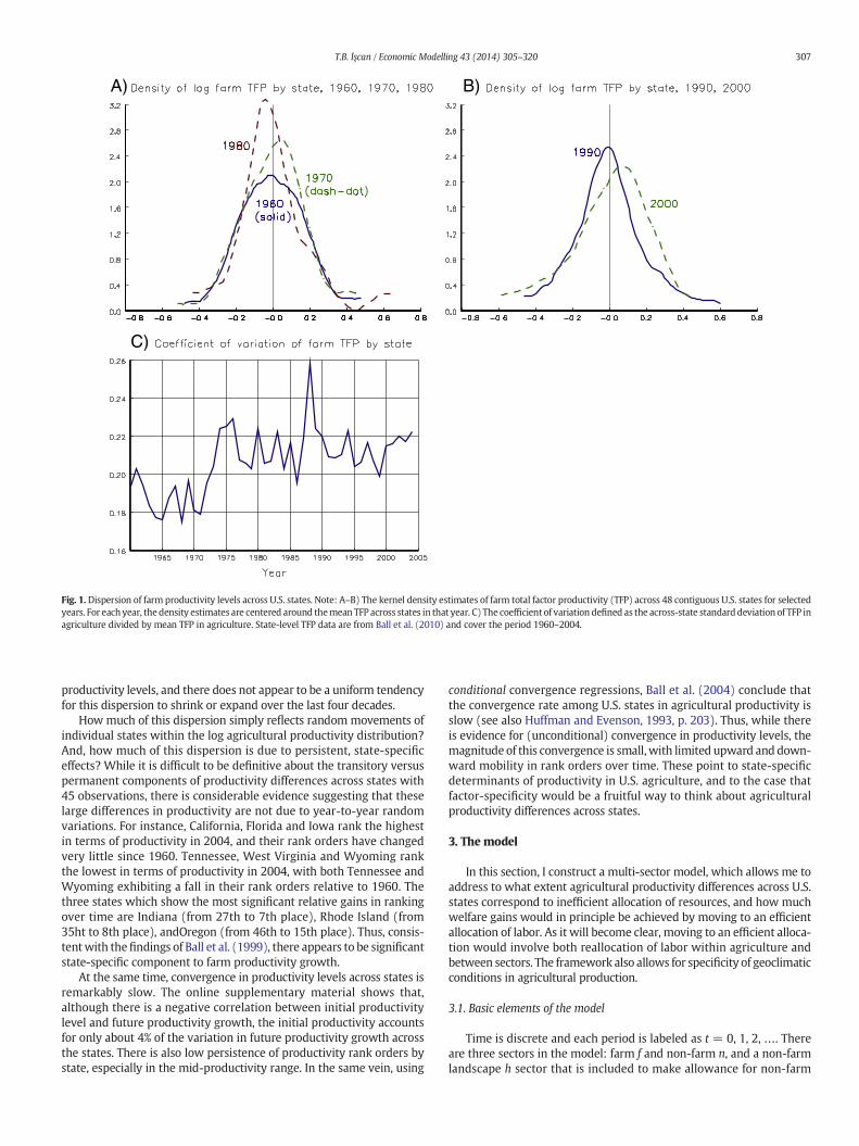
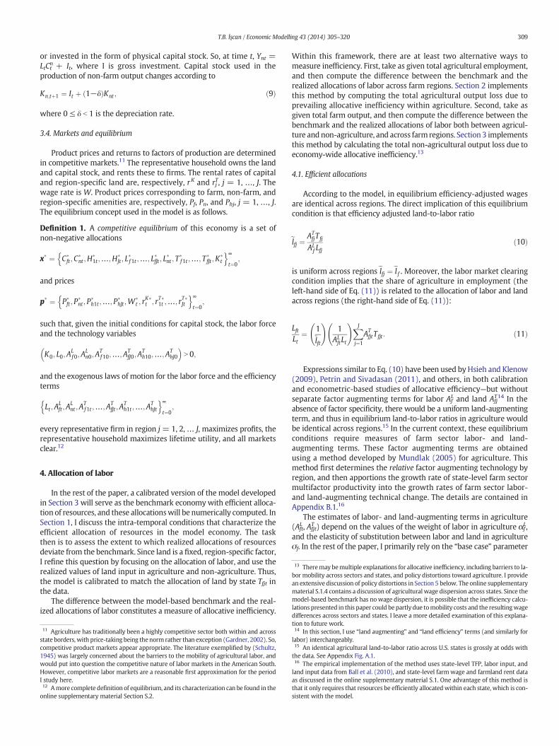
Fig. 1 plots the density estimates of log farm productivity levelsacross 48 contiguous U.S. states for five reference years: 1960, 1970,1980 (Fig. 1A), 1990, and 2000 (Fig. 1B). For ease of comparison, thedensity estimates in each year are centered around that year's meanproductivity across states (shown by the vertical line at zero). Theestimates indicate considerable dispersion in productivity levels acrossstates, with the ratio of farm productivity in the highest productivitystates to the lowest productivity states consistently exceeding 2. Forinstance, in 2004, farm productivity in California (highest ranked) washigher than in Wyoming (lowest ranked) by a factor of 3. Also, thedensity estimates suggest that the dispersion of productivity has variedover these reference years, but not in a direction that points to anysecular decrease or increase in dispersion.
I document the changes in dispersion of agricultural productivityover time by the coefficient of variation in log productivity acrossstates. Fig. 1C shows that the coefficient of variation of log agriculturalproductivity jumped noticeably in the early 1970s, but since then thismeasure of dispersion has fluctuated in a narrow band. Overall, boththe density estimates and coefficient of variation indicate that therehas been considerable dispersion across U.S. states in agricultural
5 Schultz (1945, pp. 47–49, chp. 4) argued that despite persistent differences betweenagriculture and non-agriculture in their value marginal products of labor, labor realloca-tion toward non-agriculture was slow due to “barriers” to labor mobility. See Caselli andColeman (2001) and Dennis and İşcan (2007) for quantitative assessments of the contri-bution of such channels to agricultural out-migration in the United States. Lee andWolpin(2006) investigate the contribution of labor mobility across sectors to the growth of ser-vice sector employment.
6 Unless otherwise stated, henceforth productivity refers to total factor productivity.
A) B)
C)
Fig. 1.Dispersion of farm productivity levels across U.S. states. Note: A–B) The kernel density estimates of farm total factor productivity (TFP) across 48 contiguous U.S. states for selectedyears. For each year, the density estimates are centered around themean TFP across states in that year. C) The coefficient of variation defined as the across-state standarddeviation of TFP inagriculture divided by mean TFP in agriculture. State-level TFP data are from Ball et al. (2010) and cover the period 1960–2004.
307T.B. İşcan / Economic Modelling 43 (2014) 305–320
productivity levels, and there does not appear to be a uniform tendencyfor this dispersion to shrink or expand over the last four decades.
How much of this dispersion simply reflects random movements ofindividual states within the log agricultural productivity distribution?And, how much of this dispersion is due to persistent, state-specificeffects? While it is difficult to be definitive about the transitory versuspermanent components of productivity differences across states with45 observations, there is considerable evidence suggesting that theselarge differences in productivity are not due to year-to-year randomvariations. For instance, California, Florida and Iowa rank the highestin terms of productivity in 2004, and their rank orders have changedvery little since 1960. Tennessee, West Virginia and Wyoming rankthe lowest in terms of productivity in 2004, with both Tennessee andWyoming exhibiting a fall in their rank orders relative to 1960. Thethree states which show the most significant relative gains in rankingover time are Indiana (from 27th to 7th place), Rhode Island (from35ht to 8th place), andOregon (from 46th to 15th place). Thus, consis-tentwith thefindings of Ball et al. (1999), there appears to be significantstate-specific component to farm productivity growth.
At the same time, convergence in productivity levels across states isremarkably slow. The online supplementary material shows that,although there is a negative correlation between initial productivitylevel and future productivity growth, the initial productivity accountsfor only about 4% of the variation in future productivity growth acrossthe states. There is also low persistence of productivity rank orders bystate, especially in the mid-productivity range. In the same vein, using
conditional convergence regressions, Ball et al. (2004) conclude thatthe convergence rate among U.S. states in agricultural productivity isslow (see also Huffman and Evenson, 1993, p. 203). Thus, while thereis evidence for (unconditional) convergence in productivity levels, themagnitude of this convergence is small,with limited upward and down-ward mobility in rank orders over time. These point to state-specificdeterminants of productivity in U.S. agriculture, and to the case thatfactor-specificity would be a fruitful way to think about agriculturalproductivity differences across states.
3. The model
In this section, I construct a multi-sector model, which allows me toaddress to what extent agricultural productivity differences across U.S.states correspond to inefficient allocation of resources, and how muchwelfare gains would in principle be achieved by moving to an efficientallocation of labor. As it will become clear, moving to an efficient alloca-tion would involve both reallocation of labor within agriculture andbetween sectors. The framework also allows for specificity of geoclimaticconditions in agricultural production.
3.1. Basic elements of the model
Time is discrete and each period is labeled as t = 0, 1, 2, …. Thereare three sectors in the model: farm f and non-farm n, and a non-farmlandscape h sector that is included to make allowance for non-farm
8 For non-farm landscape, the specification allows for different weights in the sub-utility function on different region-specific landscape amenities, and thus allows for pref-erences for landscape amenities that vary across regions. The elasticity of substitution inamenities across any two pairs of regions, however, is constant.
9 Non-farm intermediate inputs are a relatively small fraction of total costs in agricul-ture. In fact, from1960 to 1994, feed, seed, and livestockpurchases, all originating fromag-riculture, stand out as the most significant intermediate input into agriculture (23%), andthe cost shares of physical capital and agricultural chemicals in total agricultural costswere small at 9.4 and 6.3%, respectively (Ball et al., 1997). Thus, for modeling purposes,it is reasonable to specify a farm production function net of all intermediate inputs, and
308 T.B. İşcan / Economic Modelling 43 (2014) 305–320
land use. Let s ∈ { f, n, h} index these sectors. There are three factors ofproduction: labor L, land T, and capital K. Geographically, the economyconsists of regions,which are labeled by j∈ {1, 2,…, J}. Demographically,the economy features an infinitely-lived representative householdwhose labor force grows exogenously:
LtLt−1
¼ nt : ð1Þ
Labor is mobile across sectors and regions. Land is region specific,but otherwise can be used for producing food and non-farm amenities.Production in each sector uses a combination of labor, land, and capital.These factors are linked to value added (output net of intermediateinputs) through sectoral production functions. The farm sector uses Land region-specific T to produce food, non-farm sector uses L and K toproduce a non-food consumption good, and non-farm landscape sectoruses region-specific T to produce region-specific non-farm landscapeamenities. The representative household has preferences over theconsumption of food, the non-food good, and non-farm landscapeamenities.7
Production in each sector also depends on factor-augmentingefficiency. Let Asjt
K , AsjL , and AsjtT be the efficiency terms corresponding to
capital, labor, and land at time t in sector s and region j. These efficiencyterms change over time exogenously. Define G as the growth factor(gross growth rate):
G AXsjt
� �¼ AX
sjt
AXsj;t−1
; X ∈ K; L; Tf g: ð2Þ
Finally, define the growth rate as g(AsjtX ) = ln (G(AsjtX )).In what follows, I describe the demand and supply sides of the
economy in detail, and suppress the time variable when this causes noconfusion.
3.2. Preferences
The per person instantaneous utility function is Cobb–Douglas
u Ct ;Htð Þ ¼ ln Cηct H1−ηc
t
� �, where 0 b ηc b 1, the composite consump-
tion good C is constant elasticity of substitution (CES) across food andnon-food consumption
1−ηn� �1
ν C f−γ� �ν−1
ν þ ηn� �1
νCν−1ν
n
� � νν−1
; 0 b ηn b 1; γ ≥ 0; 0 b ν b 1;
ð3Þ
and the consumption of composite non-farm landscape H is CES acrossregion-specific landscape amenities
XJ
j¼1
ηhj� �1
μHμ−1μ
j
24 35 μμ−1
;XJ
j
ηhj ¼ 1; 0 b ηhj b 1; μ N 0: ð4Þ
The instantaneous utility function has unitary elasticity of substitu-tion between C and H, with fixed expenditure shares given by theweight parameters ηc and 1− ηc, respectively. The composite consump-tion good is non-homothetic because of subsistence (determined bythe parameter γ) nature of food consumption. Food and non-foodconsumption are gross complements and the degree of complementarydepends on the elasticity parameter ν. Expenditure shares of food (netof subsistence food consumption) and non-food depend on the weightparameters 1 − ηn and ηn, respectively. Preferences for region-specific
7 The model links sectors only through factor markets, and does not incorporate inter-mediate inputs. Thus, in themodel, food and non-food consumption originating from farmand non-farm sectors, respectively, do not directly map into their counterparts in the na-tional income and product accounts.
landscape amenities have a CES structure with weight parametersgiven by η j
h, and elasticity parameter given by μ.8
The lifetime utility function of the representative household U isadditively separable over time
X∞t¼0
βtLtu Ct ;Htð Þ; 0 b β b 1; ð5Þ
with a subjective time discount factor β.
3.3. Production
Production in each sector is characterized by a constant returns toscale production function. Production in each sector and each region isundertaken by a representative firm. Farm output in region j, Yfj, is CESbetween labor and region-specific land:9
αLf AL
f Lfj� �σ f −1
σ f þ αTf AT
fjTfj
� �σ f −1
σ f
" # σ fσ f −1
; αLf þ αT
f ¼ 1; σ f N 0: ð6Þ
The weights of labor and land in farm production depend on theparameters αf
L and αfT, respectively. The elasticity of substitution
between land and labor in farm production is σf.This specification captures two empirically relevant issues. There is
a sector-specific component to efficiency of labor in the farm sector(Af
L), but this labor efficiency term is not region specific; agriculturalknowledge and skills are mobile across farm regions. By contrast, landefficiency in agriculture (AfjT) is not only sector-specific, but is also regionspecific due to geoclimatic conditions. This is themain factor-specificitycaptured by the model.10
Non-farm output Yn is Cobb–Douglas in labor and physical capital,and does not depend on region-specific inputs:
KαKn
n ALnLn
� �αLn; αL
n þ αKn ¼ 1: ð7Þ
In non-farm production, the elasticity of substitution betweencapital and labor is unitary, and the corresponding factor weights areαnK and αn
L , respectively. Non-farm labor-efficiency term AnL can be
expressed as a function of total-factor-augmenting technology, ALn ≡
A1=αLn
n .The provision of non-farm landscape amenities in region j, Yhj, is
linear in region-specific land:
AThjThj: ð8Þ
The land-efficiency term in non-farm landscape sector AhjT is regionspecific; regions offer their idiosyncratic landscape amenities.
The outputs of farm and non-farm landscape sectors are non-durable. Only the output of the non-farm sector can be either consumed
one which only uses land and labor.10 While individual product characteristics in agriculture vary little across state borders(like different wheat and corn varieties), agriculture does not produce a homogenousproduct. In the data, the limiting factor is availability of TFP estimates at the state-product level. I will return to this issue below.
13 Theremay bemultiple explanations for allocative inefficiency, including barriers to la-bor mobility across sectors and states, and policy distortions toward agriculture. I providean extensive discussion of policy distortions in Section 5 below. The online supplementarymaterial S.1.4 contains a discussion of agricultural wage dispersion across states. Since themodel-based benchmark has no wage dispersion, it is possible that the inefficiency calcu-lations presented in this paper could be partly due tomobility costs and the resultingwagedifferences across sectors and states. I leave a more detailed examination of this explana-
309T.B. İşcan / Economic Modelling 43 (2014) 305–320
or invested in the form of physical capital stock. So, at time t, Ynt =LtCt
n + It, where I is gross investment. Capital stock used in theproduction of non-farm output changes according to
Kn;tþ1 ¼ It þ 1−δð ÞKnt ; ð9Þ
where 0 ≤ δ b 1 is the depreciation rate.
3.4. Markets and equilibrium
Product prices and returns to factors of production are determinedin competitive markets.11 The representative household owns the landand capital stock, and rents these to firms. The rental rates of capitaland region-specific land are, respectively, r K and rj
T, j = 1, …, J. Thewage rate is W. Product prices corresponding to farm, non-farm, andregion-specific amenities are, respectively, Pf, Pn, and Phj, j = 1, …, J.The equilibrium concept used in the model is as follows.
Definition 1. A competitive equilibrium of this economy is a set ofnon-negative allocations
x� ¼ C�ft ;C
�nt ;H
�1t ;…;H�
Jt ; L�f1t ;…; L�fJt ; L
�nt ; T
�f1t ;…; T�
fJt ;K�t
n o∞
t¼0;
and prices
p� ¼ P�ft ; P
�nt; P
�h1t ;…; P�
hJt ;W�t ; r
K�t ; rT�1t ;…; rT�Jt
n o∞
t¼0;
such that, given the initial conditions for capital stock, the labor forceand the technology variables
K0; L0;ALf0;A
Ln0;A
Tf10;…;AT
fJ0;ATh10;…;AT
hJ0
� �N 0;
and the exogenous laws of motion for the labor force and the efficiencyterms
Lt ;ALft ;A
Lnt ;A
Tf1t ;…;AT
fJt ;ATh1t ;…;AT
hJt
n o∞
t¼0;
every representative firm in region j = 1, 2,… J, maximizes profits, therepresentative household maximizes lifetime utility, and all marketsclear.12
4. Allocation of labor
In the rest of the paper, a calibrated version of the model developedin Section 3 will serve as the benchmark economywith efficient alloca-tion of resources, and these allocationswill be numerically computed. InSection 1, I discuss the intra-temporal conditions that characterize theefficient allocation of resources in the model economy. The taskthen is to assess the extent to which realized allocations of resourcesdeviate from the benchmark. Since land is a fixed, region-specific factor,I refine this question by focusing on the allocation of labor, and use therealized values of land input in agriculture and non-agriculture. Thus,the model is calibrated to match the allocation of land by state Tfjt inthe data.
The difference between the model-based benchmark and the real-ized allocations of labor constitutes a measure of allocative inefficiency.
11 Agriculture has traditionally been a highly competitive sector both within and acrossstate borders, with price-taking being thenorm rather than exception (Gardner, 2002). So,competitive product markets appear appropriate. The literature exemplified by (Schultz,1945) was largely concerned about the barriers to the mobility of agricultural labor, andwould put into question the competitive nature of labor markets in the American South.However, competitive labor markets are a reasonable first approximation for the periodI study here.12 Amore complete definition of equilibrium, and its characterization can be found in theonline supplementary material Section S.2.
Within this framework, there are at least two alternative ways tomeasure inefficiency. First, take as given total agricultural employment,and then compute the difference between the benchmark and therealized allocations of labor across farm regions. Section 2 implementsthis method by computing the total agricultural output loss due toprevailing allocative inefficiency within agriculture. Second, take asgiven total farm output, and then compute the difference between thebenchmark and the realized allocations of labor both between agricul-ture andnon-agriculture, and across farm regions. Section 3 implementsthis method by calculating the total non-agricultural output loss due toeconomy-wide allocative inefficiency.13
4.1. Efficient allocations
According to the model, in equilibrium efficiency-adjusted wagesare identical across regions. The direct implication of this equilibriumcondition is that efficiency adjusted land-to-labor ratio
elfj ¼ ATfjTfj
ALf Lfj
ð10Þ
is uniform across regionselfj ¼el f . Moreover, the labor market clearingcondition implies that the share of agriculture in employment (theleft-hand side of Eq. (11)) is related to the allocation of labor and landacross regions (the right-hand side of Eq. (11)):
LftLt
¼ 1~lft
!1
ALftLt
!XJ
j¼1
ATfjtTfjt : ð11Þ
Expressions similar to Eq. (10) have been used by Hsieh and Klenow(2009), Petrin and Sivadasan (2011), and others, in both calibrationand econometric-based studies of allocative efficiency—but withoutseparate factor augmenting terms for labor Af
L and land AfjT14 In the
absence of factor specificity, there would be a uniform land-augmentingterm, and thus in equilibrium land-to-labor ratios in agriculture wouldbe identical across regions.15 In the current context, these equilibriumconditions require measures of farm sector labor- and land-augmenting terms. These factor augmenting terms are obtainedusing a method developed by Mundlak (2005) for agriculture. Thismethod first determines the relative factor augmenting technology byregion, and then apportions the growth rate of state-level farm sectormultifactor productivity into the growth rates of farm sector labor-and land-augmenting technical change. The details are contained inAppendix B.1.16
The estimates of labor- and land-augmenting terms in agriculture(AftL , Afjt
T ) depend on the values of the weight of labor in agriculture αfL,
and the elasticity of substitution between labor and land in agricultureσf. In the rest of the paper, I primarily rely on the “base case” parameter
tion to future work.14 In this section, I use “land augmenting” and “land efficiency” terms (and similarly forlabor) interchangeably.15 An identical agricultural land-to-labor ratio across U.S. states is grossly at odds withthe data. See Appendix Fig. A.1.16 The empirical implementation of the method uses state-level TFP, labor input, andland input data from Ball et al. (2010), and state-level farm wage and farmland rent dataas discussed in the online supplementary material S.1. One advantage of this method isthat it only requires that resources be efficiently allocatedwithin each state, which is con-sistent with the model.
310 T.B. İşcan / Economic Modelling 43 (2014) 305–320
values that are the most common estimates available in the empiricalliterature, but I also check the robustness of the results to alternativeparameter values. These base case parameter values are: σf = 0.2 andαfL = 0.654 (see Appendix A.2 for data sources).17
The estimates of factor-augmenting efficiency also have implicationsfor the distribution of non-farm landscape amenities across U.S. states—a dimension of the data that is not targeted by the calibration. (In theonline supplementary material S.3, I derive and demonstrate theseimplications.) Overall, I find that the calibrated model implies thatNortheastern states exhibit the highest non-farm landscapeproductivityAhjT , congruent with relatively higher population density in these states
and intensive agricultural activity. By contrast, the calibrated modelimplies that Plains andMountain states have the lowest non-farm land-scape productivity, also congruent with their low population densitiesand relatively extensive agriculture.18
Another distinguishing feature of the present framework is Eq. (11),which accounts for the labor market-clearing condition. Partial equilib-rium models typically do not consider such restrictions. Incorporatingthis condition allows me to discipline the analysis by taking resourceconstraints into consideration.
4.2. Allocation of labor across U.S. states
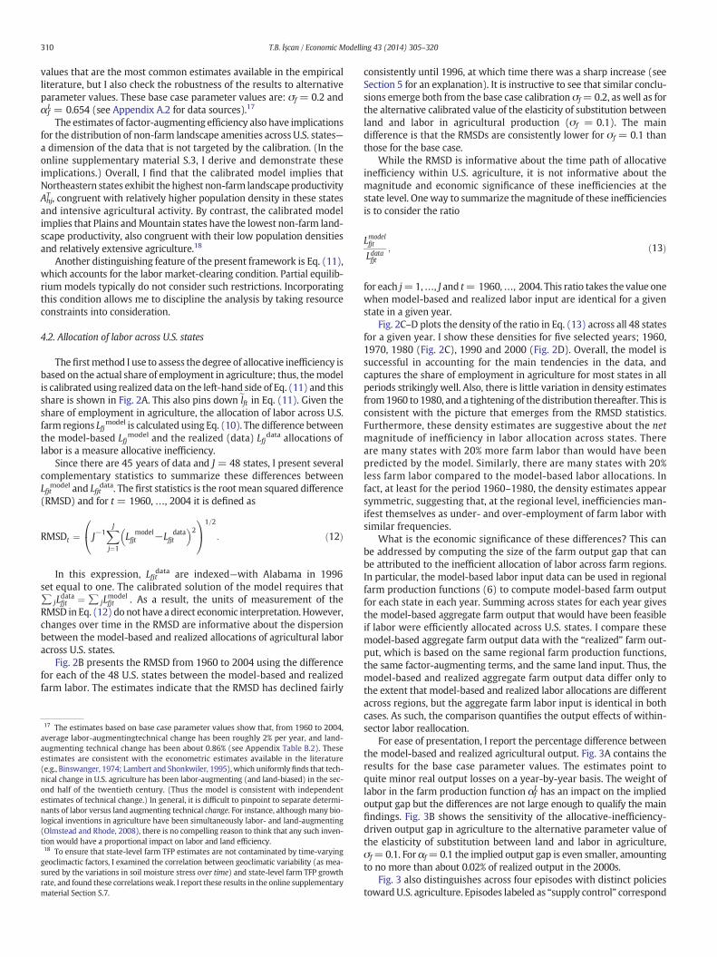
Thefirstmethod I use to assess the degree of allocative inefficiency isbased on the actual share of employment in agriculture; thus, themodelis calibrated using realized data on the left-hand side of Eq. (11) and thisshare is shown in Fig. 2A. This also pins downelft in Eq. (11). Given theshare of employment in agriculture, the allocation of labor across U.S.farm regions Lfjmodel is calculated using Eq. (10). The difference betweenthe model-based Lfj
model and the realized (data) Lfjdata allocations oflabor is a measure allocative inefficiency.
Since there are 45 years of data and J = 48 states, I present severalcomplementary statistics to summarize these differences betweenLfjt
model and Lfjtdata. The first statistics is the root mean squared difference
(RMSD) and for t = 1960,…, 2004 it is defined as
RMSDt ¼ J−1XJ
j¼1
L modelfjt −L data
fjt
� �20@ 1A1=2
: ð12Þ
In this expression, Lfjtdata are indexed—with Alabama in 1996
set equal to one. The calibrated solution of the model requires that∑ jL
datafjt ¼ ∑ jL
modelfjt . As a result, the units of measurement of the
RMSD in Eq. (12) donot have a direct economic interpretation. However,changes over time in the RMSD are informative about the dispersionbetween the model-based and realized allocations of agricultural laboracross U.S. states.
Fig. 2B presents the RMSD from 1960 to 2004 using the differencefor each of the 48 U.S. states between the model-based and realizedfarm labor. The estimates indicate that the RMSD has declined fairly
17 The estimates based on base case parameter values show that, from 1960 to 2004,average labor-augmentingtechnical change has been roughly 2% per year, and land-augmenting technical change has been about 0.86% (see Appendix Table B.2). Theseestimates are consistent with the econometric estimates available in the literature(e.g., Binswanger, 1974; Lambert and Shonkwiler, 1995), which uniformlyfinds that tech-nical change in U.S. agriculture has been labor-augmenting (and land-biased) in the sec-ond half of the twentieth century. (Thus the model is consistent with independentestimates of technical change.) In general, it is difficult to pinpoint to separate determi-nants of labor versus land augmenting technical change. For instance, althoughmany bio-logical inventions in agriculture have been simultaneously labor- and land-augmenting(Olmstead and Rhode, 2008), there is no compelling reason to think that any such inven-tion would have a proportional impact on labor and land efficiency.18 To ensure that state-level farm TFP estimates are not contaminated by time-varyinggeoclimactic factors, I examined the correlation between geoclimatic variability (as mea-sured by the variations in soil moisture stress over time) and state-level farm TFP growthrate, and found these correlationsweak. I report these results in the online supplementarymaterial Section S.7.
consistently until 1996, at which time there was a sharp increase (seeSection 5 for an explanation). It is instructive to see that similar conclu-sions emerge both from the base case calibration σf =0.2, as well as forthe alternative calibrated value of the elasticity of substitution betweenland and labor in agricultural production (σf = 0.1). The maindifference is that the RMSDs are consistently lower for σf = 0.1 thanthose for the base case.
While the RMSD is informative about the time path of allocativeinefficiency within U.S. agriculture, it is not informative about themagnitude and economic significance of these inefficiencies at thestate level. One way to summarize themagnitude of these inefficienciesis to consider the ratio
Lmodelfjt
Ldatafjt
; ð13Þ
for each j=1,…, J and t= 1960,…, 2004. This ratio takes the value onewhen model-based and realized labor input are identical for a givenstate in a given year.
Fig. 2C–D plots the density of the ratio in Eq. (13) across all 48 statesfor a given year. I show these densities for five selected years; 1960,1970, 1980 (Fig. 2C), 1990 and 2000 (Fig. 2D). Overall, the model issuccessful in accounting for the main tendencies in the data, andcaptures the share of employment in agriculture for most states in allperiods strikingly well. Also, there is little variation in density estimatesfrom1960 to 1980, and a tightening of the distribution thereafter. This isconsistent with the picture that emerges from the RMSD statistics.Furthermore, these density estimates are suggestive about the netmagnitude of inefficiency in labor allocation across states. Thereare many states with 20% more farm labor than would have beenpredicted by the model. Similarly, there are many states with 20%less farm labor compared to the model-based labor allocations. Infact, at least for the period 1960–1980, the density estimates appearsymmetric, suggesting that, at the regional level, inefficiencies man-ifest themselves as under- and over-employment of farm labor withsimilar frequencies.
What is the economic significance of these differences? This canbe addressed by computing the size of the farm output gap that canbe attributed to the inefficient allocation of labor across farm regions.In particular, the model-based labor input data can be used in regionalfarm production functions (6) to compute model-based farm outputfor each state in each year. Summing across states for each year givesthe model-based aggregate farm output that would have been feasibleif labor were efficiently allocated across U.S. states. I compare thesemodel-based aggregate farm output data with the “realized” farm out-put, which is based on the same regional farm production functions,the same factor-augmenting terms, and the same land input. Thus, themodel-based and realized aggregate farm output data differ only tothe extent that model-based and realized labor allocations are differentacross regions, but the aggregate farm labor input is identical in bothcases. As such, the comparison quantifies the output effects of within-sector labor reallocation.
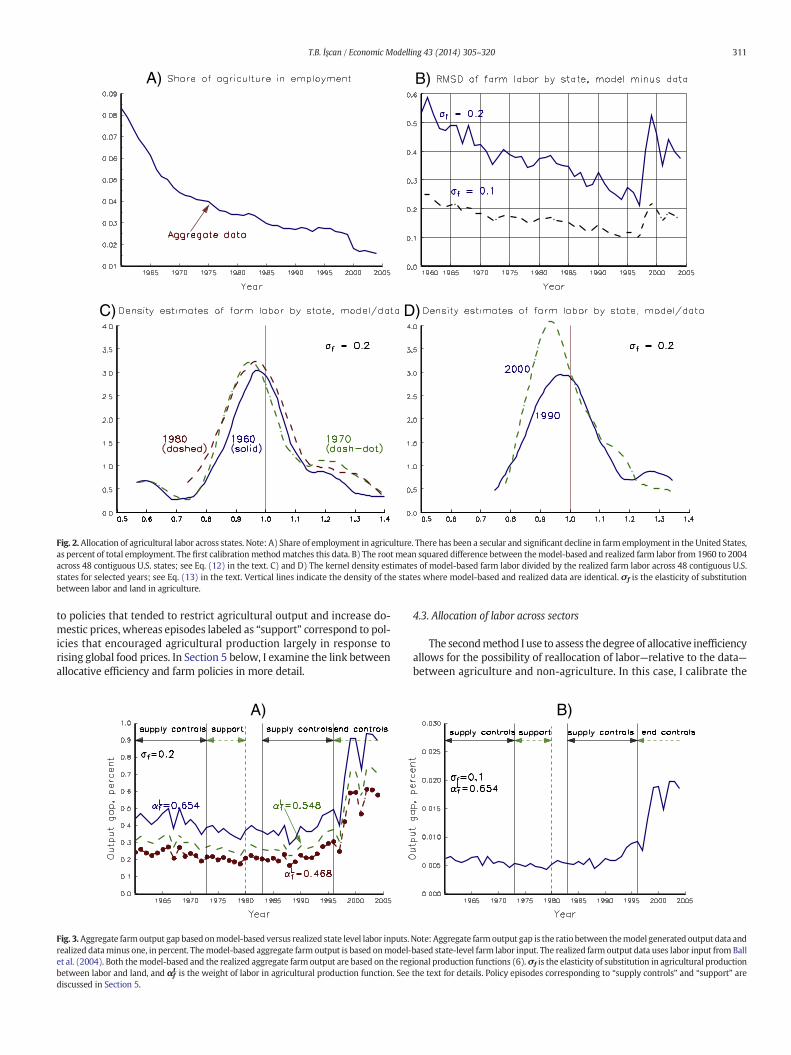
For ease of presentation, I report the percentage difference betweenthe model-based and realized agricultural output. Fig. 3A contains theresults for the base case parameter values. The estimates point toquite minor real output losses on a year-by-year basis. The weight oflabor in the farm production function αf
L has an impact on the impliedoutput gap but the differences are not large enough to qualify the mainfindings. Fig. 3B shows the sensitivity of the allocative-inefficiency-driven output gap in agriculture to the alternative parameter value ofthe elasticity of substitution between land and labor in agriculture,σf=0.1. For αf=0.1 the implied output gap is even smaller, amountingto no more than about 0.02% of realized output in the 2000s.
Fig. 3 also distinguishes across four episodes with distinct policiestoward U.S. agriculture. Episodes labeled as “supply control” correspond
A) B)
C) D)
Fig. 2. Allocation of agricultural labor across states. Note: A) Share of employment in agriculture. There has been a secular and significant decline in farm employment in the United States,as percent of total employment. The first calibrationmethodmatches this data. B) The root mean squared difference between themodel-based and realized farm labor from 1960 to 2004across 48 contiguous U.S. states; see Eq. (12) in the text. C) and D) The kernel density estimates of model-based farm labor divided by the realized farm labor across 48 contiguous U.S.states for selected years; see Eq. (13) in the text. Vertical lines indicate the density of the states where model-based and realized data are identical. σf is the elasticity of substitutionbetween labor and land in agriculture.
311T.B. İşcan / Economic Modelling 43 (2014) 305–320
to policies that tended to restrict agricultural output and increase do-mestic prices, whereas episodes labeled as “support” correspond to pol-icies that encouraged agricultural production largely in response torising global food prices. In Section 5 below, I examine the link betweenallocative efficiency and farm policies in more detail.
A)
Fig. 3.Aggregate farmoutput gap based onmodel-based versus realized state level labor inputs.realized dataminus one, in percent. Themodel-based aggregate farm output is based onmodel-et al. (2004). Both themodel-based and the realized aggregate farm output are based on the regbetween labor and land, and αf
L is the weight of labor in agricultural production function. Seediscussed in Section 5.
4.3. Allocation of labor across sectors
The secondmethod I use to assess the degree of allocative inefficiencyallows for the possibility of reallocation of labor—relative to the data—between agriculture and non-agriculture. In this case, I calibrate the
B)
Note: Aggregate farmoutput gap is the ratio between themodel generated output data andbased state-level farm labor input. The realized farm output data uses labor input from Ballional production functions (6).σf is the elasticity of substitution in agricultural productionthe text for details. Policy episodes corresponding to “supply controls” and “support” are
312 T.B. İşcan / Economic Modelling 43 (2014) 305–320
model to match aggregate farm output in the data. Under an efficientallocation of labor across farm regions, farm output in the data can beproduced with fewer farm workers. This gives rise to reallocation oflabor from the farm to the non-farm sector, and to higher non-farmoutput relative to the data. Therefore, this method considers theemployment options of labor outside the agricultural sector.
Relative to the first method, this approach comes closer to measur-ing the general equilibrium ramifications of allocative inefficiency in amulti-sector framework: it allows for the allocation of labor both acrossfarm regions and across sectors, after imposing the condition thatYftmodel = Y ft
data19 I then compare themodel-based share of employmentin agriculture
Lmodelft
Lt¼X J
j¼1Lmodelfjt
Lt;
with the realized (data) share of employment in agriculture
Ldataft
Lt¼X J
j¼1Ldatafjt
Lt:
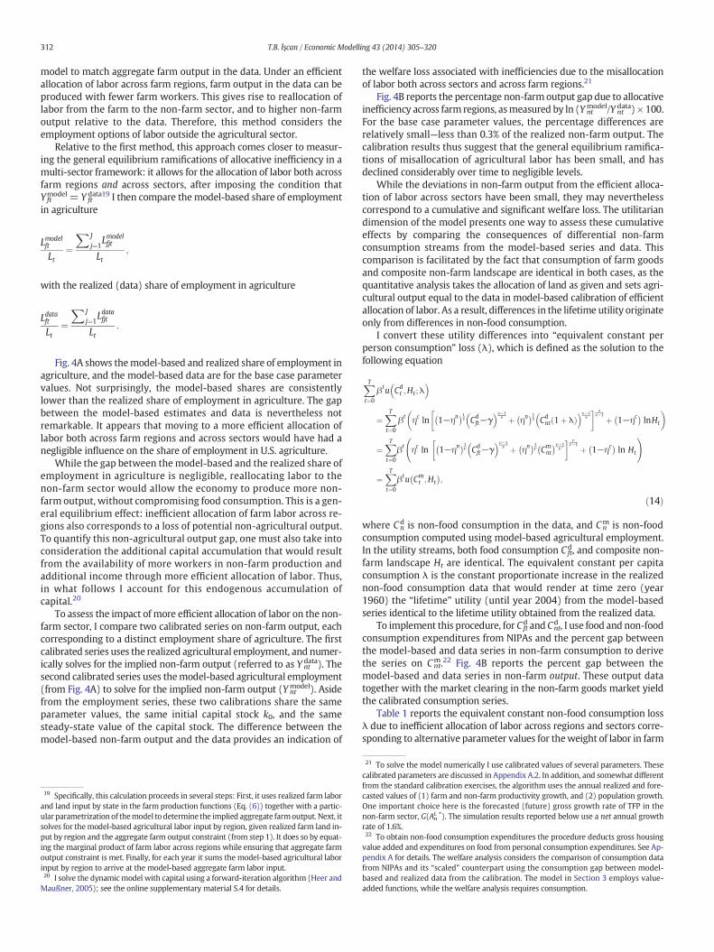
Fig. 4A shows themodel-based and realized share of employment inagriculture, and the model-based data are for the base case parametervalues. Not surprisingly, the model-based shares are consistentlylower than the realized share of employment in agriculture. The gapbetween the model-based estimates and data is nevertheless notremarkable. It appears that moving to a more efficient allocation oflabor both across farm regions and across sectors would have had anegligible influence on the share of employment in U.S. agriculture.
While the gap between themodel-based and the realized share ofemployment in agriculture is negligible, reallocating labor to thenon-farm sector would allow the economy to produce more non-farm output, without compromising food consumption. This is a gen-eral equilibrium effect: inefficient allocation of farm labor across re-gions also corresponds to a loss of potential non-agricultural output.To quantify this non-agricultural output gap, one must also take intoconsideration the additional capital accumulation that would resultfrom the availability of more workers in non-farm production andadditional income through more efficient allocation of labor. Thus,in what follows I account for this endogenous accumulation ofcapital.20
To assess the impact of more efficient allocation of labor on the non-farm sector, I compare two calibrated series on non-farm output, eachcorresponding to a distinct employment share of agriculture. The firstcalibrated series uses the realized agricultural employment, and numer-ically solves for the implied non-farm output (referred to as Y nt
data). Thesecond calibrated series uses themodel-based agricultural employment(from Fig. 4A) to solve for the implied non-farm output (Y nt
model). Asidefrom the employment series, these two calibrations share the sameparameter values, the same initial capital stock k0, and the samesteady-state value of the capital stock. The difference between themodel-based non-farm output and the data provides an indication of
19 Specifically, this calculation proceeds in several steps: First, it uses realized farm laborand land input by state in the farm production functions (Eq. (6)) together with a partic-ular parametrization of themodel to determine the implied aggregate farmoutput. Next, itsolves for themodel-based agricultural labor input by region, given realized farm land in-put by region and the aggregate farm output constraint (from step 1). It does so by equat-ing the marginal product of farm labor across regions while ensuring that aggregate farmoutput constraint is met. Finally, for each year it sums the model-based agricultural laborinput by region to arrive at the model-based aggregate farm labor input.20 I solve the dynamicmodel with capital using a forward-iteration algorithm (Heer andMaußner, 2005); see the online supplementary material S.4 for details.
the welfare loss associated with inefficiencies due to the misallocationof labor both across sectors and across farm regions.21
Fig. 4B reports the percentage non-farm output gap due to allocativeinefficiency across farm regions, asmeasured by ln (Y nt
model/Y ntdata) × 100.
For the base case parameter values, the percentage differences arerelatively small—less than 0.3% of the realized non-farm output. Thecalibration results thus suggest that the general equilibrium ramifica-tions of misallocation of agricultural labor has been small, and hasdeclined considerably over time to negligible levels.
While the deviations in non-farm output from the efficient alloca-tion of labor across sectors have been small, they may neverthelesscorrespond to a cumulative and significant welfare loss. The utilitariandimension of the model presents one way to assess these cumulativeeffects by comparing the consequences of differential non-farmconsumption streams from the model-based series and data. Thiscomparison is facilitated by the fact that consumption of farm goodsand composite non-farm landscape are identical in both cases, as thequantitative analysis takes the allocation of land as given and sets agri-cultural output equal to the data in model-based calibration of efficientallocation of labor. As a result, differences in the lifetime utility originateonly from differences in non-food consumption.
I convert these utility differences into “equivalent constant perperson consumption” loss (λ), which is defined as the solution to thefollowing equation
XTt¼0
βtu Cdt ;Ht ;λ
� �
¼XTt¼0
βt ηc ln 1−ηn� �1
v Cdft−γ
� �v−1v þ ηn
� �1v Cd
nt 1þ λð Þ� �v−1
v
� � vv−1 þ 1−ηc
� �lnHt
�
¼XTt¼0
βt ηc ln 1−ηn� �1
ν Cdft−γ
� �ν−1ν þ ηn
� �1ν Cm
nt
� �ν−1ν
� � νν−1 þ 1−ηc
� �ln Ht
!
¼XTt¼0
βtu Cmt ;Ht
� �;
ð14Þ
where Cnd is non-food consumption in the data, and Cn
m is non-foodconsumption computed using model-based agricultural employment.In the utility streams, both food consumption C ft
d, and composite non-farm landscape Ht are identical. The equivalent constant per capitaconsumption λ is the constant proportionate increase in the realizednon-food consumption data that would render at time zero (year1960) the “lifetime” utility (until year 2004) from the model-basedseries identical to the lifetime utility obtained from the realized data.
To implement this procedure, for Cftd and Cnt
d , I use food and non-foodconsumption expenditures from NIPAs and the percent gap betweenthe model-based and data series in non-farm consumption to derivethe series on Cnt
m.22 Fig. 4B reports the percent gap between themodel-based and data series in non-farm output. These output datatogether with the market clearing in the non-farm goods market yieldthe calibrated consumption series.
Table 1 reports the equivalent constant non-food consumption lossλ due to inefficient allocation of labor across regions and sectors corre-sponding to alternative parameter values for theweight of labor in farm
21 To solve the model numerically I use calibrated values of several parameters. Thesecalibrated parameters are discussed in Appendix A.2. In addition, and somewhat differentfrom the standard calibration exercises, the algorithm uses the annual realized and fore-casted values of (1) farm and non-farm productivity growth, and (2) population growth.One important choice here is the forecasted (future) gross growth rate of TFP in thenon-farm sector, G(An
L ⁎). The simulation results reported below use a net annual growthrate of 1.6%.22 To obtain non-food consumption expenditures the procedure deducts gross housingvalue added and expenditures on food from personal consumption expenditures. See Ap-pendix A for details. The welfare analysis considers the comparison of consumption datafrom NIPAs and its “scaled” counterpart using the consumption gap between model-based and realized data from the calibration. The model in Section 3 employs value-added functions, while the welfare analysis requires consumption.
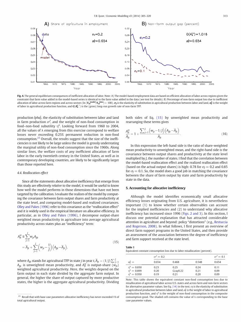
A) B)
Fig. 4.The general equilibrium consequences of inefficient allocation of labor. Note: A) Themodel-based employment data are based on efficient allocation of labor across regions given theconstraint that farm value added in the model-based series is identical to the farm value added in the data (see text for details). B) Percentage of non-farm output loss due to inefficientallocation of labor across farm regions and across sectors (ln (Ynt
model/Yntdata) × 100).σf is the elasticity of substitution in agricultural production between labor and land,αf
L is theweightof labor in agricultural production function, and G(An
L ⁎) is the (gross) long-run growth rate of non-farm TFP.
Table 1Equivalent constant consumption loss due to labor misallocation (percent).
σ f = 0.2 σ f = 0.1
αfL = 0.654 0.468 0.548 0.654
ηn = 0.850 0.23 0.25 0.24 0.11ηn = 0.899 0.20 Gray0.22 0.21 0.09ηn = 0.950 0.19 0.21 0.20 0.09
Note: This table shows the equivalent constant non-food consumption loss due tomisallocation of agricultural labor across U.S. states and across farm and non-farm sectors
313T.B. İşcan / Economic Modelling 43 (2014) 305–320
production lphafL, the elasticity of substitution between labor and land
in farm production σ f, and the weight of non-food consumption infood–non-food subutility ηn. Looking forward from 1960 to 2004,all the values of λ emerging from this exercise correspond to welfarelosses never exceeding 0.25% permanent reduction in non-foodconsumption.23 Overall, the results suggest that the size of the ineffi-ciencies is not likely to be large unless themodel is grossly understatingthe marginal utility of non-food consumption since the 1960s. Alongsimilar lines, the welfare costs of any inefficient allocation of farmlabor in the early twentieth century in the United States, as well as incontemporary developing countries, are likely to be significantly largerthan those reported here.
4.4. Reallocation effect
Since all the statements about allocative inefficiency that emerge fromthis study are effectively relative to themodel, it would be useful to knowhow well the model performs in those dimensions that have not beentargeted by the calibration. I evaluate the realismof themodel by comput-ing the covariance between farm output shares and farm productivity atthe state level, and comparing model-based and realized covariances.Olley and Pakes (1996) refer to this covariance as the “reallocation effect”and it is widely used in the empirical literature on allocative efficiency. Inparticular, as in Olley and Pakes (1996), I decompose output-shareweighted mean productivity in agriculture into average agriculturalproductivity across states plus an “inefficiency” term:
Awft ≡
XJ
j¼1
wjtAfjt
¼ Aft þXJ
j¼1
wjt−1J
� Afjt−Aft
� �;
ð15Þ
where Afjt stands for agricultural TFP in state j in year t,Aft ¼ 1= Jð Þ∑ Jj¼1
Afjt is unweighted mean productivity, and Aftw is output-share (wjt)
weighted agricultural productivity. Here, the weights depend on thefarm output in each state divided by the aggregate farm output. Ingeneral, the higher the share of output captured by more productivestates, the higher is the aggregate agricultural productivity. Dividing
23 Recall that with base case parameters allocative inefficiency has never exceeded 1% oftotal agricultural output.
both sides of Eq. (15) by unweighted mean productivity andrearranging these terms gives
Awft
Aft
¼ 1þX J
j¼1wjt−1= J� �
Afjt−Aft
� �Aft
: ð16Þ
In this expression the left-hand side is the ratio of share-weightedmean productivity to unweighted mean, and the right-hand side is thecovariance between output shares and productivity at the state levelmultiplied by J, the number of states. I find that the correlation betweenthe model-based reallocation effect and the realized reallocation effect(based on the actual output shares) is high: 0.78 for σf = 0.2 and 0.85for σf = 0.1. So, the model does a good job in matching the covariancebetween the share of farm output by state and farm productivity bystate in the data.
5. Accounting for allocative inefficiency
Although the model identifies economically small allocativeefficiency losses originating from U.S. agriculture, it is neverthelessimportant (1) to know whether certain observables can accountfor the implied inefficiencies and (2) to understand why allocativeinefficiency has increased since 1996 (Figs. 2 and 3). In this section, Idiscuss one potential explanation that has attracted considerableattention in agriculture and beyond: policy “distortions” (e.g., Restucciaand Rogerson, 2008). In what follows, I first present an overview ofdirect farm support programs in the United States, and then providean assessment of the association between the degree of inefficiencyand farm support received at the state level.
for alternative parameter values. See Eq. (14) in the text. σf is the elasticity of substitutionin agricultural production between labor and land, αf
L is the weight of labor in agriculturalproduction function, and ηn is the weight of non-food consumption in the compositeconsumption good. The shaded cell contains the value of λ corresponding to the basecase parameter values.
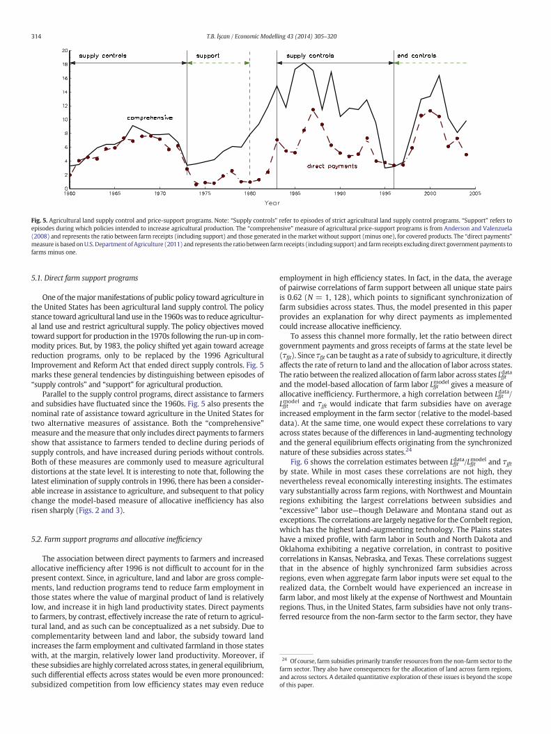
Fig. 5. Agricultural land supply control and price-support programs. Note: “Supply controls” refer to episodes of strict agricultural land supply control programs. “Support” refers toepisodes during which policies intended to increase agricultural production. The “comprehensive” measure of agricultural price-support programs is from Anderson and Valenzuela(2008) and represents the ratio between farm receipts (including support) and those generated in the market without support (minus one), for covered products. The “direct payments”measure is based onU.S.Department of Agriculture (2011) and represents the ratio between farm receipts (including support) and farm receipts excluding direct governmentpayments tofarms minus one.
314 T.B. İşcan / Economic Modelling 43 (2014) 305–320
5.1. Direct farm support programs
One of themajormanifestations of public policy toward agriculture inthe United States has been agricultural land supply control. The policystance toward agricultural land use in the 1960swas to reduce agricultur-al land use and restrict agricultural supply. The policy objectives movedtoward support for production in the 1970s following the run-up in com-modity prices. But, by 1983, the policy shifted yet again toward acreagereduction programs, only to be replaced by the 1996 AgriculturalImprovement and Reform Act that ended direct supply controls. Fig. 5marks these general tendencies by distinguishing between episodes of“supply controls” and “support” for agricultural production.
Parallel to the supply control programs, direct assistance to farmersand subsidies have fluctuated since the 1960s. Fig. 5 also presents thenominal rate of assistance toward agriculture in the United States fortwo alternative measures of assistance. Both the “comprehensive”measure and themeasure that only includes direct payments to farmersshow that assistance to farmers tended to decline during periods ofsupply controls, and have increased during periods without controls.Both of these measures are commonly used to measure agriculturaldistortions at the state level. It is interesting to note that, following thelatest elimination of supply controls in 1996, there has been a consider-able increase in assistance to agriculture, and subsequent to that policychange the model-based measure of allocative inefficiency has alsorisen sharply (Figs. 2 and 3).
24 Of course, farm subsidies primarily transfer resources from the non-farm sector to thefarm sector. They also have consequences for the allocation of land across farm regions,and across sectors. A detailed quantitative exploration of these issues is beyond the scopeof this paper.
5.2. Farm support programs and allocative inefficiency
The association between direct payments to farmers and increasedallocative inefficiency after 1996 is not difficult to account for in thepresent context. Since, in agriculture, land and labor are gross comple-ments, land reduction programs tend to reduce farm employment inthose states where the value of marginal product of land is relativelylow, and increase it in high land productivity states. Direct paymentsto farmers, by contrast, effectively increase the rate of return to agricul-tural land, and as such can be conceptualized as a net subsidy. Due tocomplementarity between land and labor, the subsidy toward landincreases the farm employment and cultivated farmland in those stateswith, at the margin, relatively lower land productivity. Moreover, ifthese subsidies are highly correlated across states, in general equilibrium,such differential effects across states would be even more pronounced:subsidized competition from low efficiency states may even reduce
employment in high efficiency states. In fact, in the data, the averageof pairwise correlations of farm support between all unique state pairsis 0.62 (N = 1, 128), which points to significant synchronization offarm subsidies across states. Thus, the model presented in this paperprovides an explanation for why direct payments as implementedcould increase allocative inefficiency.
To assess this channel more formally, let the ratio between directgovernment payments and gross receipts of farms at the state level be(τfjt). Since τfjt can be taught as a rate of subsidy to agriculture, it directlyaffects the rate of return to land and the allocation of labor across states.The ratio between the realized allocation of farm labor across states Lfjtdata
and the model-based allocation of farm labor Lfjtmodel gives a measure ofallocative inefficiency. Furthermore, a high correlation between Lfjt
data/Lfjtmodel and τjft would indicate that farm subsidies have on averageincreased employment in the farm sector (relative to the model-baseddata). At the same time, one would expect these correlations to varyacross states because of the differences in land-augmenting technologyand the general equilibrium effects originating from the synchronizednature of these subsidies across states.24
Fig. 6 shows the correlation estimates between Lfjtdata/Lfjtmodel and τjft
by state. While in most cases these correlations are not high, theynevertheless reveal economically interesting insights. The estimatesvary substantially across farm regions, with Northwest and Mountainregions exhibiting the largest correlations between subsidies and“excessive” labor use—though Delaware and Montana stand out asexceptions. The correlations are largely negative for the Cornbelt region,which has the highest land-augmenting technology. The Plains stateshave a mixed profile, with farm labor in South and North Dakota andOklahoma exhibiting a negative correlation, in contrast to positivecorrelations in Kansas, Nebraska, and Texas. These correlations suggestthat in the absence of highly synchronized farm subsidies acrossregions, even when aggregate farm labor inputs were set equal to therealized data, the Cornbelt would have experienced an increase infarm labor, and most likely at the expense of Northwest and Mountainregions. Thus, in the United States, farm subsidies have not only trans-ferred resource from the non-farm sector to the farm sector, they have
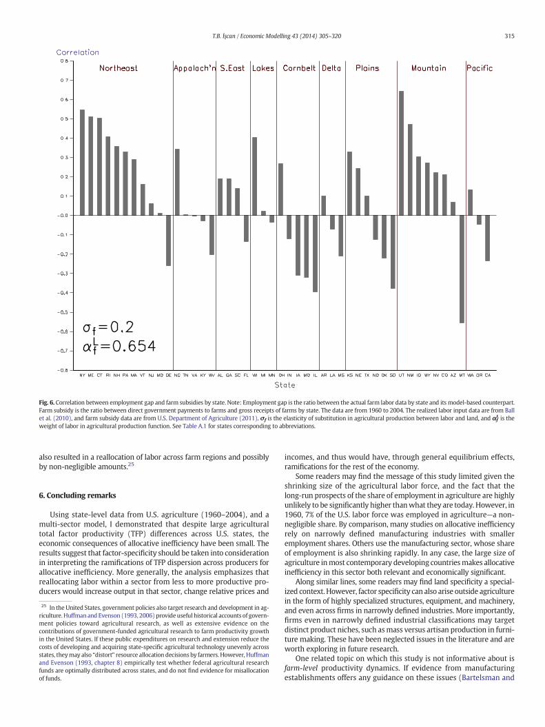
Fig. 6. Correlation between employment gap and farm subsidies by state. Note: Employment gap is the ratio between the actual farm labor data by state and its model-based counterpart.Farm subsidy is the ratio between direct government payments to farms and gross receipts of farms by state. The data are from 1960 to 2004. The realized labor input data are from Ballet al. (2010), and farm subsidy data are from U.S. Department of Agriculture (2011). σf is the elasticity of substitution in agricultural production between labor and land, and αf
L is theweight of labor in agricultural production function. See Table A.1 for states corresponding to abbreviations.
315T.B. İşcan / Economic Modelling 43 (2014) 305–320
also resulted in a reallocation of labor across farm regions and possiblyby non-negligible amounts.25
6. Concluding remarks
Using state-level data from U.S. agriculture (1960–2004), and amulti-sector model, I demonstrated that despite large agriculturaltotal factor productivity (TFP) differences across U.S. states, theeconomic consequences of allocative inefficiency have been small. Theresults suggest that factor-specificity should be taken into considerationin interpreting the ramifications of TFP dispersion across producers forallocative inefficiency. More generally, the analysis emphasizes thatreallocating labor within a sector from less to more productive pro-ducers would increase output in that sector, change relative prices and
25 In the United States, government policies also target research and development in ag-riculture. Huffman and Evenson (1993, 2006) provide useful historical accounts of govern-ment policies toward agricultural research, as well as extensive evidence on thecontributions of government-funded agricultural research to farm productivity growthin the United States. If these public expenditures on research and extension reduce thecosts of developing and acquiring state-specific agricultural technology unevenly acrossstates, theymay also “distort” resource allocation decisions by farmers. However, Huffmanand Evenson (1993, chapter 8) empirically test whether federal agricultural researchfunds are optimally distributed across states, and do not find evidence for misallocationof funds.
incomes, and thus would have, through general equilibrium effects,ramifications for the rest of the economy.
Some readers may find the message of this study limited given theshrinking size of the agricultural labor force, and the fact that thelong-run prospects of the share of employment in agriculture are highlyunlikely to be significantly higher thanwhat they are today. However, in1960, 7% of the U.S. labor force was employed in agriculture—a non-negligible share. By comparison, many studies on allocative inefficiencyrely on narrowly defined manufacturing industries with smalleremployment shares. Others use the manufacturing sector, whose shareof employment is also shrinking rapidly. In any case, the large size ofagriculture inmost contemporary developing countriesmakes allocativeinefficiency in this sector both relevant and economically significant.
Along similar lines, some readers may find land specificity a special-ized context. However, factor specificity can also arise outside agriculturein the form of highly specialized structures, equipment, and machinery,and even across firms in narrowly defined industries. More importantly,firms even in narrowly defined industrial classifications may targetdistinct product niches, such asmass versus artisan production in furni-ture making. These have been neglected issues in the literature and areworth exploring in future research.
One related topic on which this study is not informative about isfarm-level productivity dynamics. If evidence from manufacturingestablishments offers any guidance on these issues (Bartelsman and
Table A.1State abbreviations.
State Abb. State Abb. State Abb. State Abb.
Alabama AL Iowa IA Nebraska NE Rhode Island RIArizona AZ Kansas KS Nevada NV South Carolina SCArkansas AR Kentucky KY New Hampshire NH South Dakota SDCalifornia CA Louisiana LA New Jersey NJ Tennessee TNColorado CO Maine ME New Mexico NM Texas TXConnecticut CT Maryland MD New York NY Utah UTDelaware DE Massachusetts MA North Carolina NC Vermont VTFlorida FL Michigan MI North Dakota ND Virginia VAGeorgia GA Minnesota MN Ohio OH Washington WAIdaho ID Mississippi MS Oklahoma OK West Virginia WVIllinois IL Missouri MO Oregon OR Wisconsin WIIndiana IN Montana MT Pennsylvania PA Wyoming WY
316 T.B. İşcan / Economic Modelling 43 (2014) 305–320
Doms, 2000), productivity levels across farmswithin a state are likely tobe quite dispersed as well. Yet, available aggregate data are notinformative about farm-level productivity dynamics, including the con-tribution of entering and exiting farms to observed state-level produc-tivity growth rates. Moreover, the analysis here focuses on a singleagricultural good with the implication that, in an efficient equilibrium,the ratios of marginal value product of efficiency-adjusted labor andland should be identical across regions. However, specialization incrop versus livestock production, with their distinct specialized factorsraises additional issues that have not been pursued in this paper, largelydue to data limitations.26 Thus, future extensions along these linesappear fruitful.
An additional avenue for future research is paying careful attentionto intermediate inputs and input–output table style interactions acrossand within sectors (e.g., Basu et al., 2010). Such extensions would helpalign more carefully the model-based consumption and productionconcepts with their empirical counterparts in national income andproduct accounts, and would deliver richer channels of resourcereallocation.
Appendix A. Data
The data are annual for 48 contiguous U.S. states. In the model, eachtime period corresponds to a calendar year, and each region corre-sponds to a U.S. state. State abbreviations are listed in Table A.1.
A.1. Variables
A.1.1. Farm and non-farm TFP growthThe data on multifactor productivity Ant in the non-farm sector and
regional Afjt in the farm sector are available as index numbers derivedusing standard productivity measurement techniques, and the datasources are:
Ant: Private non-farm business sector (excluding governmententerprises) multifactor productivity is from the U.S. Bureau ofLabor Statistics (2011).
Aft: State-level farm sector multifactor productivity estimates are for48-contiguous states and from the U.S. Department of Agriculture,Economic Research Service. See Ball et al. (2010) for data, documen-tation, and methods.
A.1.2. State-level labor and land inputsThese data are are from Ball et al. (2010). The methodology used by
USDA to measure state-level TFP controls for cross-state differences insoil quality in determining land input (Ball et al., 2010). Soil quality
26 See the online supplementary material S.6 for additional discussion.
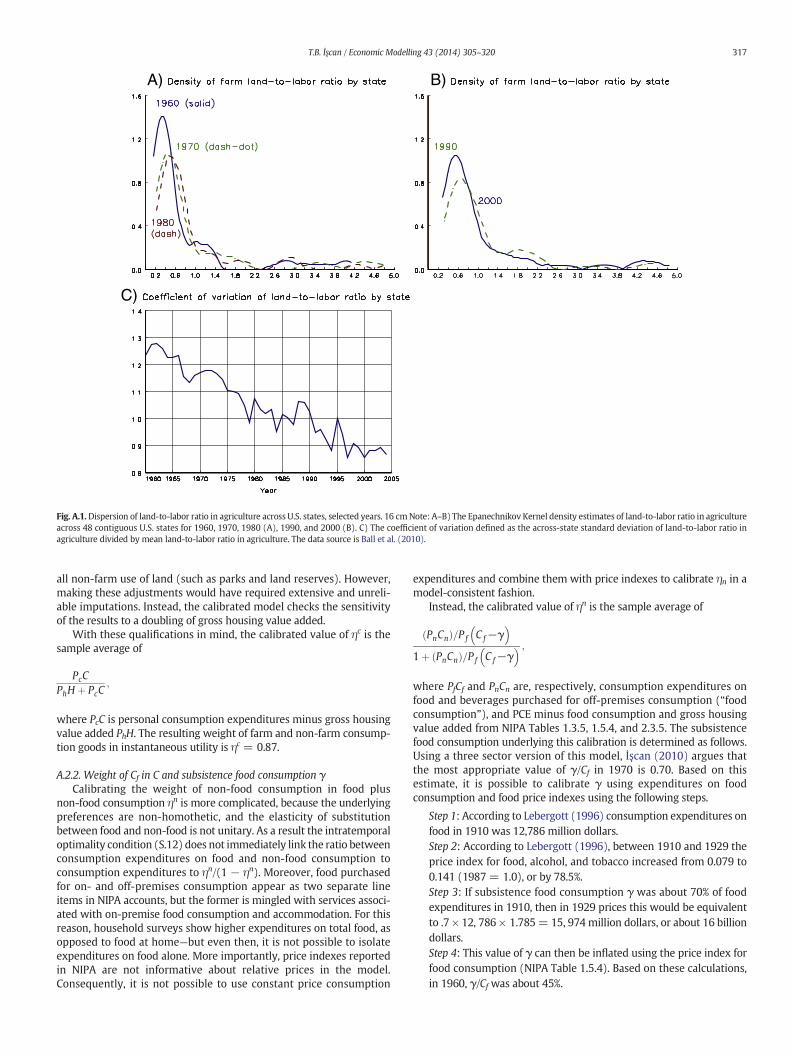
assessment is based on Beinroth et al. (2001), who group land in sixquality classes based on a combination of soil performance and soilresilience criteria for grain production. As such, the TFP measurescontrol for state-level fixed effects based on soil quality. Fig. A.1 plotsthe density estimates of farmland-to-labor ratio for five selected years.
A.1.3. State-level farm wage and farmland rentSee the online supplementary material S.1.
A.1.4. Aggregate sectoral employmentFarm (“agriculture”) and total civilian non-institutional employ-
ment are from the Current Population Survey and are based on house-hold surveys (U.S. Bureau of Labor Statistics, Table 1: Employmentstatus of the civilian noninstitutional population, 1940 to date, http://www.bls.gov/data/home.htm, accessed 2 May 2011). The governmentemployment data are from the Current Employment Statistics and arebased on establishment surveys (http://www.bls.gov/ces/cesbtabs.htm, accessed 2May2011). For forecasts of nt, t N T, I use population pro-jections for ages 16 years and over from the Census Bureau (2004).
A.2. Calibration
The elasticity of substitution in consumption between farm and non-farm goods is ν = 0.1 (following Dennis and İşcan, 2009). The timediscount factor β = 0.943 and the depreciation rate δ = 0.065are from Gomme and Rupert (2007). The remaining parameters arecalibrated as follows.
A.2.1. Weight of C in consumption ηc
To calibrate theweight of food plus non-food consumption C in totalconsumption including non-farm landscape ηc, I use the intratemporaloptimality condition (S.11), which states that the ratio betweenconsumption expenditures on food plus non-food and consumptionexpenditures on non-farm landscape be equal to ηc/(1 − ηc). Bothexpenditure items are difficult to map into available data. Expenditureson food and non-food consumption would be best captured by thepersonal consumption expenditures (PCE) as reported by the U.S.Department of Commerce, Bureau of Economic Analysis (BEA http://www.bea.gov, accessed June 6, 2011), in the National Income andProduct Accounts (NIPA), Table 2.3.5. But, this includes expenditureson durable goods and housing. Although the model does not tacklethe distinct issues related to the consumption of services from durablegoods, I include them in non-food consumption expenditures. Expendi-tures on housing in part capture expenditures on non-farm landscape,so I deduct gross housing value added (NIPA Table 1.3.5) from PCE.Gross housing value added mingles housing services and value of non-farm land, so it overestimates consumption expenditures on non-farmland alone. At the same time, it underestimates expenditures on non-farm landscape, because it does not include the gross value added by
A)
C)
B)
Fig. A.1. Dispersion of land-to-labor ratio in agriculture across U.S. states, selected years. 16 cmNote: A–B) The Epanechnikov Kernel density estimates of land-to-labor ratio in agricultureacross 48 contiguous U.S. states for 1960, 1970, 1980 (A), 1990, and 2000 (B). C) The coefficient of variation defined as the across-state standard deviation of land-to-labor ratio inagriculture divided by mean land-to-labor ratio in agriculture. The data source is Ball et al. (2010).
317T.B. İşcan / Economic Modelling 43 (2014) 305–320
all non-farm use of land (such as parks and land reserves). However,making these adjustments would have required extensive and unreli-able imputations. Instead, the calibrated model checks the sensitivityof the results to a doubling of gross housing value added.
With these qualifications in mind, the calibrated value of ηc is thesample average of
PcCPhH þ PcC
;
where PcC is personal consumption expenditures minus gross housingvalue added PhH. The resulting weight of farm and non-farm consump-tion goods in instantaneous utility is ηc = 0.87.
A.2.2. Weight of Cf in C and subsistence food consumption γCalibrating the weight of non-food consumption in food plus
non-food consumption ηn is more complicated, because the underlyingpreferences are non-homothetic, and the elasticity of substitutionbetween food and non-food is not unitary. As a result the intratemporaloptimality condition (S.12) does not immediately link the ratio betweenconsumption expenditures on food and non-food consumption toconsumption expenditures to ηn/(1 − ηn). Moreover, food purchasedfor on- and off-premises consumption appear as two separate lineitems in NIPA accounts, but the former is mingled with services associ-ated with on-premise food consumption and accommodation. For thisreason, household surveys show higher expenditures on total food, asopposed to food at home—but even then, it is not possible to isolateexpenditures on food alone. More importantly, price indexes reportedin NIPA are not informative about relative prices in the model.Consequently, it is not possible to use constant price consumption
expenditures and combine them with price indexes to calibrate ηn in amodel-consistent fashion.
Instead, the calibrated value of ηn is the sample average of
PnCnð Þ=P f C f−γ� �
1þ PnCnð Þ=P f C f−γ� � ;
where PfCf and PnCn are, respectively, consumption expenditures onfood and beverages purchased for off-premises consumption (“foodconsumption”), and PCE minus food consumption and gross housingvalue added from NIPA Tables 1.3.5, 1.5.4, and 2.3.5. The subsistencefood consumption underlying this calibration is determined as follows.Using a three sector version of this model, İşcan (2010) argues thatthe most appropriate value of γ/Cf in 1970 is 0.70. Based on thisestimate, it is possible to calibrate γ using expenditures on foodconsumption and food price indexes using the following steps.
Step 1: According to Lebergott (1996) consumption expenditures onfood in 1910 was 12,786 million dollars.Step 2: According to Lebergott (1996), between 1910 and 1929 theprice index for food, alcohol, and tobacco increased from 0.079 to0.141 (1987 = 1.0), or by 78.5%.Step 3: If subsistence food consumption γ was about 70% of foodexpenditures in 1910, then in 1929 prices this would be equivalentto .7 × 12, 786 × 1.785= 15, 974 million dollars, or about 16 billiondollars.Step 4: This value of γ can then be inflated using the price index forfood consumption (NIPA Table 1.5.4). Based on these calculations,in 1960, γ/Cf was about 45%.
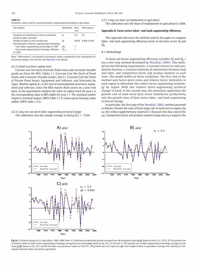
Table B.1Parameter values used for measuring factor-augmenting technology in agriculture.
Description Mnemonic Basecase
Alternatives
Elasticity of substitution in farm productionbetween labor and land
σf 0.2 0.1
Weight of labor in farm production αfL 0.654 0.468, 0.548
Normalization of factor-augmenting technologyFarm labor-augmenting technology in 1960 Af,0
L 1Farm land-augmenting technology, Alabama
in 1960Af,1,0T 1
Note: “Alternatives” correspond to parameter values considered in the simulations forsensitivity analysis. See the text and Appendix A for details.
318 T.B. İşcan / Economic Modelling 43 (2014) 305–320
A.2.3. Initial non-farm capital stockCurrent-cost net stock of private fixed assets and consumer durable
goods are from the BEA, Tables 1.1 (Current-Cost Net Stock of FixedAssets and Consumer Durable Goods) and 2.1 (Current-Cost Net Stockof Private Fixed Assets, Equipment and Software, and Structures byType). Market capital, Kn, is the sum of nonresidential structures, equip-ment and software. Since the BEA reports fixed assets on a year-endbasis, in the quantitative analysis the value of capital stock for year t isthe corresponding value in BEA tables for year t-1. The nominal marketoutput is nominal output (NIPA Table 1.1.5) minus gross housing valueadded (NIPA Table 1.3.5).
A.2.4. Long-run non-farm labor-augmenting technical changeThe calibration uses the sample average so that g(AnL) = 1.634.
A)
C)
Fig. B.1. Technical change inU.S. agriculture, 1960–2004. Note: A) Total factor productivity growof relative (labor-to-land) factor-augmenting technology averaged across states g(af) based onstates g(Af
L) based on Eq. (B.3) and for the base case parameter values in Table B.1. All growthstitution between labor and land in agriculture.
A.2.5. Long-run share of employment in agricultureThe calibration uses the share of employment in agriculture in 2004.
Appendix B. Farm sector labor- and land-augmenting efficiency
This appendix discusses the method used in the paper to computelabor- and land-augmenting efficiency terms in the farm sector Aft
L andAfjtT .
B.1. Methodology
To back-out factor-augmenting efficiency variables AftL and Afjt
T , Iuse a two-step method developed by Mundlak (2005). This meth-od has the following requirements: a constant returns to scale pro-duction function, a constant elasticity of substitution between landand labor, and competitive factor and product markets in eachstate. The model builds on these conditions. The first step of themethod uses factor-price ratios and relative factor intensities ineach region to determine the relative factor augmenting technolo-gy by region. With this relative factor-augmenting technicalchange in hand, in the second step, the procedure apportions thegrowth rate of state-level farm sector multifactor productivityinto the growth rates of farm sector labor- and land-augmentingtechnical change.
In particular, the first step of the Mundlak (2005) method proceedsas follows. Denote the ratio of farm wage rate to land rent in region j byωj (the online supplementarymaterial S.1 discusses the data sources forωj). Competitive factor and productmarkets imply thatωj is equal to the
B)
th averaged over 48 contiguous states g(Af) based on Ball et al. (2010). B) The growth rateEq. (B.2) in the text. C) The growth rate of labor-augmenting technology averaged acrossrates are in percent. αf
L is the weight of labor in agriculture, and σf is the elasticity of sub-
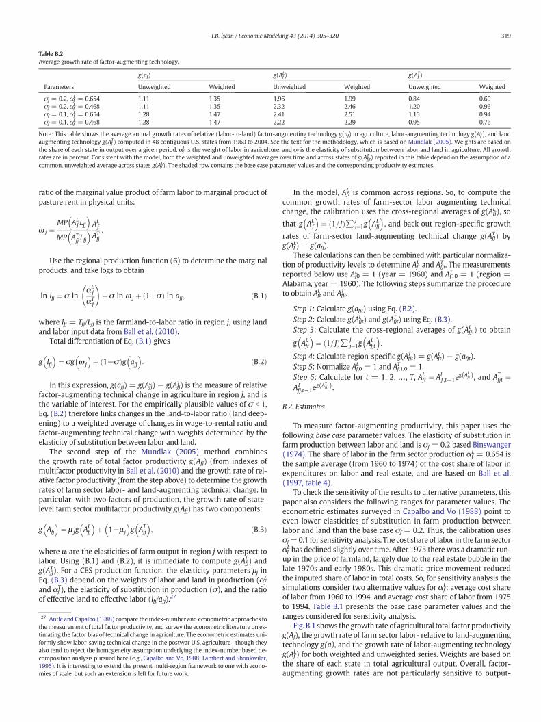
Table B.2Average growth rate of factor-augmenting technology.
g(af) g(AfL) g(Af
T)
Parameters Unweighted Weighted Unweighted Weighted Unweighted Weighted
σf = 0.2, αfL = 0.654 1.11 1.35 1.96 1.99 0.84 0.60
σf = 0.2, αfL = 0.468 1.11 1.35 2.32 2.46 1.20 0.96
σf = 0.1, αfL = 0.654 1.28 1.47 2.41 2.51 1.13 0.94
σf = 0.1, αfL = 0.468 1.28 1.47 2.22 2.29 0.95 0.76
Note: This table shows the average annual growth rates of relative (labor-to-land) factor-augmenting technology g(af) in agriculture, labor-augmenting technology g(AfL), and land
augmenting technology g(AfT) computed in 48 contiguous U.S. states from 1960 to 2004. See the text for the methodology, which is based on Mundlak (2005). Weights are based on
the share of each state in output over a given period. αfL is the weight of labor in agriculture, and σf is the elasticity of substitution between labor and land in agriculture. All growth
rates are in percent. Consistent with the model, both the weighted and unweighted averages over time and across states of g(AfjtT ) reported in this table depend on the assumption of acommon, unweighted average across states g(AfL). The shaded row contains the base case parameter values and the corresponding productivity estimates.
319T.B. İşcan / Economic Modelling 43 (2014) 305–320
ratio of themarginal value product of farm labor to marginal product ofpasture rent in physical units:
ω j ¼MP AL
f Lfj� �
MP ATfjTfj
� �ALf
ATfj
:
Use the regional production function (6) to determine the marginalproducts, and take logs to obtain
ln lfj ¼ σ lnαL
f
αTf
!þ σ ln ω j þ 1−σð Þ ln afj; ðB:1Þ
where lfj = Tfj/Lfj is the farmland-to-labor ratio in region j, using landand labor input data from Ball et al. (2010).
Total differentiation of Eq. (B.1) gives
g lfj� �
¼ σg ω j
� �þ 1−σð Þg afj
� �: ðB:2Þ
In this expression, g(afj) = g(AfjL) − g(AfjT) is the measure of relative
factor-augmenting technical change in agriculture in region j, and isthe variable of interest. For the empirically plausible values of σ b 1,Eq. (B.2) therefore links changes in the land-to-labor ratio (land deep-ening) to a weighted average of changes in wage-to-rental ratio andfactor-augmenting technical change with weights determined by theelasticity of substitution between labor and land.
The second step of the Mundlak (2005) method combinesthe growth rate of total factor productivity g(Afj) (from indexes ofmultifactor productivity in Ball et al. (2010) and the growth rate of rel-ative factor productivity (from the step above) to determine the growthrates of farm sector labor- and land-augmenting technical change. Inparticular, with two factors of production, the growth rate of state-level farm sector multifactor productivity g(Afj) has two components:
g Afj
� �¼ μ jg AL
fj
� �þ 1−μ j
� �g AT
fj
� �; ðB:3Þ
where μj are the elasticities of farm output in region j with respect tolabor. Using (B.1) and (B.2), it is immediate to compute g(Afj
L) andg(Afj
T). For a CES production function, the elasticity parameters μj inEq. (B.3) depend on the weights of labor and land in production (αf
L
and αfT), the elasticity of substitution in production (σ), and the ratio
of effective land to effective labor (lfj/afj).27
27 Antle and Capalbo (1988) compare the index-number and econometric approaches tothemeasurement of total factor productivity, and survey the econometric literature on es-timating the factor bias of technical change in agriculture. The econometric estimates uni-formly show labor-saving technical change in the postwar U.S. agriculture—though theyalso tend to reject the homogeneity assumption underlying the index-number based de-composition analysis pursued here (e.g., Capalbo and Vo, 1988; Lambert and Shonkwiler,1995). It is interesting to extend the present multi-region framework to one with econo-mies of scale, but such an extension is left for future work.
In the model, AftL is common across regions. So, to compute the
common growth rates of farm-sector labor augmenting technicalchange, the calibration uses the cross-regional averages of g(Afj
L), so
that g ALf
� �¼ 1= Jð Þ∑ J
j¼1g ALfj
� �, and back out region-specific growth
rates of farm-sector land-augmenting technical change g(AfjT) by
g(AfL) − g(afj).These calculations can then be combined with particular normaliza-
tion of productivity levels to determine AftL and Afjt
T . The measurementsreported below use Af0
L = 1 (year = 1960) and Af10T = 1 (region =
Alabama, year = 1960). The following steps summarize the procedureto obtain Aft
L and AfjtT .
Step 1: Calculate g(afjt) using Eq. (B.2).Step 2: Calculate g(AfjtL ) and g(AfjtT ) using Eq. (B.3).Step 3: Calculate the cross-regional averages of g(Afjt
L ) to obtain
g ALft
� �¼ 1= Jð Þ∑ J
j¼1g ALfjt
� �:
Step 4: Calculate region-specific g(AfjtT ) = g(AftL) − g(afjt).Step 5: Normalize Af,0
L = 1 and Af,1,0T = 1.
Step 6: Calculate for t = 1, 2, …, T, ALft ¼ AL
f ;t−1eg AL
ftð Þ, and ATfjt ¼
ATfj;t−1e
g ATfjtð Þ.
B.2. Estimates
To measure factor-augmenting productivity, this paper uses thefollowing base case parameter values. The elasticity of substitution infarm production between labor and land is σf = 0.2 based Binswanger(1974). The share of labor in the farm sector production αf
L = 0.654 isthe sample average (from 1960 to 1974) of the cost share of labor inexpenditures on labor and real estate, and are based on Ball et al.(1997, table 4).
To check the sensitivity of the results to alternative parameters, thispaper also considers the following ranges for parameter values. Theeconometric estimates surveyed in Capalbo and Vo (1988) point toeven lower elasticities of substitution in farm production betweenlabor and land than the base case σf = 0.2. Thus, the calibration usesσf=0.1 for sensitivity analysis. The cost share of labor in the farm sectorαfL has declined slightly over time. After 1975 there was a dramatic run-
up in the price of farmland, largely due to the real estate bubble in thelate 1970s and early 1980s. This dramatic price movement reducedthe imputed share of labor in total costs. So, for sensitivity analysis thesimulations consider two alternative values for αf
L: average cost shareof labor from 1960 to 1994, and average cost share of labor from 1975to 1994. Table B.1 presents the base case parameter values and theranges considered for sensitivity analysis.
Fig. B.1 shows the growth rate of agricultural total factor productivityg(Af), the growth rate of farm sector labor- relative to land-augmentingtechnology g(a), and the growth rate of labor-augmenting technologyg(AfL) for both weighted and unweighted series. Weights are based onthe share of each state in total agricultural output. Overall, factor-augmenting growth rates are not particularly sensitive to output-
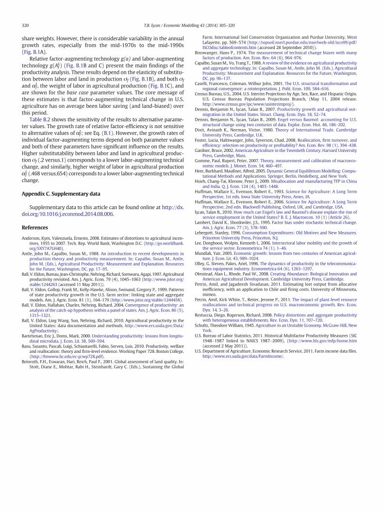
320 T.B. İşcan / Economic Modelling 43 (2014) 305–320
share weights. However, there is considerable variability in the annualgrowth rates, especially from the mid-1970s to the mid-1990s(Fig. B.1A).
Relative factor-augmenting technology g(a) and labor-augmentingtechnology g(Af
L) (Fig. B.1B and C) present the main findings of theproductivity analysis. These results depend on the elasticity of substitu-tion between labor and land in production σf (Fig. B.1B), and both σf
and αfL, the weight of labor in agricultural production (Fig. B.1C), and
are shown for the base case parameter values. The core message ofthese estimates is that factor-augmenting technical change in U.S.agriculture has on average been labor saving (and land-biased) overthis period.
Table B.2 shows the sensitivity of the results to alternative parame-ter values. The growth rate of relative factor-efficiency is not sensitiveto alternative values of αf
L; see Eq. (B.1). However, the growth rates ofindividual factor-augmenting terms depend on both parameter valuesand both of these parameters have significant influence on the results.Higher substitutability between labor and land in agricultural produc-tion σf (.2 versus.1) corresponds to a lower labor-augmenting technicalchange, and similarly, higher weight of labor in agricultural productionαfL (.468 versus.654) corresponds to a lower labor-augmenting technical
change.
Appendix C. Supplementary data
Supplementary data to this article can be found online at http://dx.doi.org/10.1016/j.econmod.2014.08.006.
References
Anderson, Kym, Valenzuela, Ernesto, 2008. Estimates of distortions to agricultural incen-tives, 1955 to 2007. Tech. Rep. World Bank, Washington D.C. (http://go.worldbank.org/5XY7A7LH40).
Antle, John M., Capalbo, Susan M., 1988. An introduction to recent developments inproduction theory and productivity measurement. In: Capalbo, Susan M., Antle,John M. (Eds.), Agricultural Productivity: Measurement and Explanation. Resourcesfor the Future, Washington, DC, pp. 17–95.
Ball, V. Eldon, Bureau, Jean-Christophe,Nehring, Richard, Somwaru, Agapi, 1997. Agriculturalproductivity revisited. Am. J. Agric. Econ. 79 (4), 1045–1063 (http://www.jstor.org/stable/1244263 (accessed 11 May 2011)).
Ball, V. Eldon, Gollop, Frank M., Kelly-Hawke, Alison, Swinand, Gregory P., 1999. Patternsof state productivity growth in the U.S. farm sector: linking state and aggregatemodels. Am. J. Agric. Econ. 81 (1), 164–179 (http://www.jstor.org/stable/1244458).
Ball, V. Eldon, Hallahan, Charles, Nehring, Richard, 2004. Convergence of productivity: ananalysis of the catch-up hypothesis within a panel of states. Am. J. Agric. Econ. 86 (5),1315–1321.
Ball, V. Eldon, Ling Wang, Sun, Nehring, Richard, 2010. Agricultural productivity in theUnited States: data documentation and methods. http://www.ers.usda.gov/Data/AgProductivity/.
Bartelsman, Eric J., Doms, Mark, 2000. Understanding productivity: lessons from longitu-dinal microdata. J. Econ. Lit. 38, 569–594.
Basu, Susanto, Pascali, Luigi, Schiantarelli, Fabio, Serven, Luis, 2010. Productivity, welfareand reallocation: theory and firm-level evidence.Working Paper 728. Boston College,(http://fmwww.bc.edu/ec-p/wp728.pdf).
Beinroth, F.H., Eswaran, Hari, Reich, Paul F., 2001. Global assessment of land quality. In:Stott, Diane E., Mohtar, Rabi H., Steinhardt, Gary C. (Eds.), Sustaining the Global
Farm. International Soil Conservation Organization and Purdue University, WestLafayette, pp. 569–574 (http://topsoil.nserl.purdue.edu/nserlweb-old/isco99/pdf/ISCOdisc/tableofcontents.htm (accessed 28 September 2010)).
Binswanger, Hans P., 1974. The measurement of technical change biases with manyfactors of production. Am. Econ. Rev. 64 (6), 964–976.
Capalbo, SusanM., Vo, Trang T., 1988. A review of the evidence on agricultural productivityand aggregate technology. In: Capalbo, Susan M., Antle, John M. (Eds.), AgriculturalProductivity: Measurement and Explanation. Resources for the Future, Washington,DC, pp. 96–137.
Caselli, Francesco, Coleman, Wilbur John, 2001. The U.S. structural transformation andregional convergence: a reinterpretation. J. Polit. Econ. 109, 584–616.
Census Bureau, U.S., 2004. U.S. Interim Projections by Age, Sex, Race, and Hispanic Origin.U.S. Census Bureau Population Projections Branch, (May 11, 2004 release.http://www.census.gov/ipc/www/usinterimproj/).
Dennis, Benjamin N., İşcan, Talan B., 2007. Productivity growth and agricultural out-migration in the United States. Struct. Chang. Econ. Dyn. 18, 52–74.
Dennis, Benjamin N., İşcan, Talan B., 2009. Engel versus Baumol: accounting for U.S.structural change using two centuries of data. Explor. Econ. Hist. 46, 186–202.
Dixit, Avinash K., Norman, Victor, 1980. Theory of International Trade. CambridgeUniversity Press, Cambridge, U.K.
Foster, Lucia, Haltiwanger, John, Syverson, Chad, 2008. Reallocation, firm turnover, andefficiency: selection on productivity or profitability? Am. Econ. Rev. 98 (1), 394–438.
Gardner, Bruce, 2002. American Agriculture in the Twentieth Century. Harvard UniversityPress, Cambridge, Mass.
Gomme, Paul, Rupert, Peter, 2007. Theory, measurement and calibration of macroeco-nomic models. J. Monet. Econ. 54, 460–497.
Heer, Burkhard, Maußner, Alfred, 2005. Dynamic General EquilibriumModelling: Compu-tational Methods and Applications. Springer, Berlin, Heidelberg, and New York.
Hsieh, Chang-Tai, Klenow, Peter J., 2009. Misallocation and manufacturing TFP in Chinaand India. Q. J. Econ. 124 (4), 1403–1448.
Huffman, Wallace E., Evenson, Robert E., 1993. Science for Agriculture: A Long TermPerspective, 1st edn. Iowa State University Press, Ames, IA.
Huffman, Wallace E., Evenson, Robert E., 2006. Science for Agriculture: A Long TermPerspective, 2nd edn. Blackwell Publishing, Oxford, UK, and Cambridge, USA.
İşcan, Talan B., 2010. How much can Engel's law and Baumol's disease explain the rise ofservice employment in the United States? B. E. J. Macroecon. 10 (1) (Article 26).
Lambert, David K., Shonkwiler, J.S., 1995. Factor bias under stochastic technical change.Am. J. Agric. Econ. 77 (3), 578–590.
Lebergott, Stanley, 1996. Consumption Expenditures: Old Motives and New Measures.Princeton University Press, Princeton, N.J.
Lee, Donghoon, Wolpin, Kenneth I., 2006. Intersectoral labor mobility and the growth ofthe service sector. Econometrica 74 (1), 1–46.
Mundlak, Yair, 2005. Economic growth: lessons from two centuries of American agricul-ture. J. Econ. Lit. 43, 989–1024.
Olley, G. Steven, Pakes, Ariel, 1996. The dynamics of productivity in the telecommunica-tions equipment industry. Econometrica 64 (6), 1263–1297.
Olmstead, Alan L., Rhode, Paul W., 2008. Creating Abundance: Biological Innovation andAmerican Agricultural Development. Cambridge University Press, Cambridge.
Petrin, Amil, and Jagadeesh Sivadasan, 2011. Estimating lost output from allocativeinefficiency, with an application to Chile and firing costs. University of Minnesota,mimeo.
Petrin, Amil, Kirk White, T., Reiter, Jerome P., 2011. The impact of plant-level resourcereallocations and technical progress on U.S. macroeconomic growth. Rev. Econ.Dyn. 14, 3–26.
Restuccia, Diego, Rogerson, Richard, 2008. Policy distortions and aggregate productivitywith heterogeneous establishments. Rev. Econ. Dyn. 11, 707–720.
Schultz, TheodoreWilliam, 1945. Agriculture in an Unstable Economy. McGraw-Hill, NewYork.
U.S. Bureau of Labor Statistics, 2011. Historical Multifactor Productivity Measures (SIC1948–1987 linked to NAICS 1987–2009), (http://www.bls.gov/mfp/home.htm(accessed 2 May 2011)).
U.S. Department of Agriculture, Economic Research Service, 2011. Farm income data files.http://www.ers.usda.gov/data/FarmIncome/.