DEA 2004 1

Algorithms on words

• Elementary algorithms

• Tries and automata

• Pattern matching

• Transducers

• Parsing

•Word enumeration

• Probability distributions on words

• Statistics on words

DEA 2004 2

Elementary algorithms

• The class Alphabet

• Overlaps and borders

• Factors

• Subwords

• Conjugates and Lyndon words

• The class ElementaryAlgorithms

DEA 2004 3

Alphabets and words

ε

a b

aa ab ba bb

aaa aab aba abb baa bab bba bbb

· · · · · ·

Figure 1: The tree of the free monoid on two letters.

DEA 2004 4

Ordered alphabets

1

10 11

100 101 110 111

1000 1001 1010 1011 1100 1101 1110 1111

· · · · · ·

Figure 2: The tree of integers in binary notation.

DEA 2004 5

Distances

a b b a b a a b

a b a a b a b a

(a) Hamming distancea b b a b a a b

a b a a b a b a

(b) Subword dis-tance

Figure 3: The Hamming distance is 3 and the subword

distance is 2.

DEA 2004 6

b aa b a b b aa b b a b aa b a b b a b aa b b aa b a b b a

a b b a b aa b b aa b a b b a b aa b a b b aa b b a b aa b

Figure 4: The Hamming distance of these two Thue-

Morse blocks of length 32 is equal to their length,

their subword distance is only 6.

DEA 2004 7

The class Alphabet

This class implements the alphabet. Internally, for

automata, grammars or transducers, the alphabet

is always a set of consecutive short integers begin-

ning with 0. An alphabet can be created using

several constructors among which:

• Alphabet(char letter, int n) for an al-

phabet of size n beginning at character letter

• Alphabet(Set charSet) from a given set of

characters.

Moreover the method fromFile(String name)

returns the alphabet of characters appearing in the

file name. The basic elements of an alphabet are

the methods

• int size() which is the number of elements

of the alphabet.

• short toShort(char c) to convert to the

internal representation and

• char toChar(int i) to convert backwords.

DEA 2004 8

Overlaps and borders

The overlap of x and y is the longest proper suffix

of x that is also a proper prefix of y. Forexample,

the overlap of abacaba and acabaca has length 5.

The border of a non empty word w is the overlap

of w and itself.

border(xa) =

{

ua if ua is a prefix of x,

border(ua) otherwise.

For example, if x = abaababa, the array b is

0 1 2 3 4 5 6 7 8

b : -1 0 0 1 1 2 3 2 3

Border(x)

1 . x has length m, b has size m + 1

2 i← 0

3 b[0]← −1

4 for j ← 1 to m− 1 do

5 b[j]← i

6 . Here x[0..i− 1] = border(x[0..j − 1])

7 while i ≥ 0 and x[j] 6= x[i] do

8 i← b[i]

9 i← i + 1

10 b[m]← i

11 return b

DEA 2004 9

Complexity: linear since j + (j − i) increases

stricly at each iteration.

DEA 2004 10

Factors

j

y : w u a z

x : u b t

x : u′ c t′

iFigure 5: Checking x[i] against y[j].

SearchFactor(x, y)

1 . x has length m, y has length n

2 . b is the array of length of borders of the prefixes of x

3 b← Border(x)

4 (i, j)← (0, 0)

5 while i < m and j < n do

6 while i ≥ 0 and x[i] 6= y[j] do

7 i← b[i]

8 (i, j)← (i + 1, j + 1)

9 return i = m

Complexity: O(|x| + |y|).

DEA 2004 11

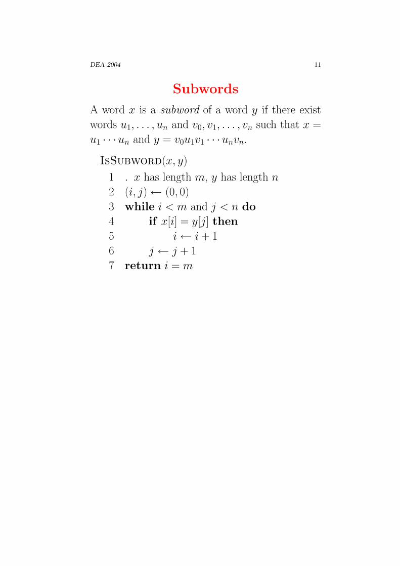
Subwords

A word x is a subword of a word y if there exist

words u1, . . . , un and v0, v1, . . . , vn such that x =

u1 · · ·un and y = v0u1v1 · · ·unvn.

IsSubword(x, y)

1 . x has length m, y has length n

2 (i, j)← (0, 0)

3 while i < m and j < n do

4 if x[i] = y[j] then

5 i← i + 1

6 j ← j + 1

7 return i = m

DEA 2004 12

Longest common subword

lcs(xa, yb) =

{

lcs(x, y)a if a = b,

max(lcs(xa, y), lcs(x, yb)) otherwise.

a b a b

0 0 0 0 0

a 0 1 1 1 1

b 0 1 2 2 2

b 0 1 2 2 3

a 0 1 2 3 3

M [i+1, j+1] =

{

M [i, j] + 1 if x[i] = y[j],

max(M [i + 1, j], M [i, j + 1]) otherwise.

LcsLengthArray(x, y)

1 . x has length m and y has length n

2 for i← 0 to m− 1 do

3 for j ← 0 to n− 1 do

4 if x[i] = y[j] then

5 M [i + 1, j + 1]←M [i, j] + 1

6 else M [i + 1, j + 1]← max(M [i + 1, j], M [i, j + 1])

7 return M

Complexity: quadratic.

DEA 2004 13

To recover an lcs:

Lcs(x, y)

1 . result is a word w

2 M ← LcsLengthArray(x, y)

3 (i, j, k)← (m− 1, n− 1, M [m, n]− 1)

4 while k ≥ 0 do

5 if x[i] = y[j] then

6 w[k]← x[i]

7 (i, j, k)← (i− 1, j − 1, k − 1)

8 else if M [i + 1, j] < M [i, j + 1] then

9 i← i− 1

10 else j ← j − 1

11 return w

DEA 2004 14

Conjugates and Lyndon words

k + jk + j − i

x

k

x0 k + i

Figure 6: Checking whether x[k..k+m−1] is the least

circular conjugate of x.

CircularMin(x)

1 (i, j, k)← (0, 1, 0)

2 b[0]← −1

3 while k + j < 2m do

4 . Here x[k..k + i− 1] = border(x[k..k + j − 1])

5 if j − i = m then

6 return k

7 b[j]← i

8 while i ≥ 0 and x[k + j] 6= x[k + i] do

9 if x[k + j] < x[k + i] then

10 (k, j)← (k + j − i, i)

11 i← b[i]

12 (i, j)← (i + 1, j + 1)

Complexity: linear

DEA 2004 15

Lyndon factorization

For any word x, there is a unique factorization

x = `n11· · · `nr

r

where r ≥ 0, n1, . . . , nr ≥ 1, and `1 > · · · > `r

are Lyndon words.

LyndonFactorization(x)

1 . x has length m

2 (i, j)← (0, 1)

3 while j < m and x[i] ≤ x[j] do

4 if x[i] < x[j] then

5 i← 0

6 else i← i + 1

7 j ← j + 1

8 return (j − i, bj/(j − i)c)Complexity: linear.

DEA 2004 16

The class ElementaryAlgorithms

This class implements the elementary algorithms

on words of Section 1.2. These include string-

matching algorithms, subwords with longest com-

mon subwords and conjugacy with minimal cyclic

conjugate and Lyndon factorization. Usage:

java ElementaryAlgorithms command word1

(opt) word2

where command can be one of

border to print the border array of word1

borderSharp to print the sharp border array of

word1

circularMin to print the least conjugate of word1

lyndonFact to print the Lyndon factorization of

word1

lcsArray to print the array of lengths of the longest

common subwords of word1 and word2

lcs to print a longest common subword of word1

and word2

For example, the command

java ElementaryAlgorithms border abracadabra

produces the output

-1 0 0 0 1 0 1 0 1 2 3 4

The command

java ElementaryAlgorithms circularMin abracadabra

DEA 2004 17

produces

aabracadab

The command

java ElementaryAlgorithms lyndonFact abracadabra

produces

0

7

10

(abracad)(abr)(a)

The command

java ElementaryAlgorithms lcs abracadabra

arbadacarba

produces

aradara

DEA 2004 18

Tries and automata

• Tries

• The interface Trie

• The class VariableArrayTrie

• Automata

• The classes NFA and DFA

• The classes INFA and IDFA

• Determinization of automata

• Minimization of automata

DEA 2004 19

Tries

1

2l

3

s

4e

5e

6a7

t

8n

9d

10t

11t

12e

13e

14r

15r

Figure 7: A trie

IsInTrie(w)

1 . checks if the word w of length n is in the trie

2 (i, p)← LongestPrefixInTrie(w)

3 return i = n and p is a terminal vertex

LongestPrefixInTrie(w)

1 . returns the length of the longest prefix of w

2 . in the trie, and the vertex reached by this prefix.

3 q ← Root()

4 i← 0

5 do p← q

6 q ← Next(q, w[i])

7 i← i + 1

8 while q 6= −1 and i < n

9 return (i− 1, p)

DEA 2004 20

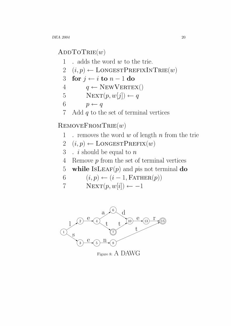
AddToTrie(w)

1 . adds the word w to the trie.

2 (i, p)← LongestPrefixInTrie(w)

3 for j ← i to n− 1 do

4 q ← NewVertex()

5 Next(p, w[j])← q

6 p← q

7 Add q to the set of terminal vertices

RemoveFromTrie(w)

1 . removes the word w of length n from the trie

2 (i, p)← LongestPrefix(w)

3 . i should be equal to n

4 Remove p from the set of terminal vertices

5 while IsLeaf(p) and pis not terminal do

6 (i, p)← (i− 1,Father(p))

7 Next(p, w[i])← −1

1

2l

3

s

4e

5e

6a

7

t

8n

d10

tt

13e

15r

Figure 8: A DAWG

DEA 2004 21

The interface Trie

Interface for the implementation of the Trie data

structure. This interface is implemented by the

following classes:

• FixedArrayTrie in which each node is an

array of fixed size of pointers to its sons.

• VariableArrayTrie in which each node is an

array of variable size of pointers to its sons.

• ForaxTrie in which each is an array of vari-

able size of pointers to its sons. The list of sons

is ordered by the label.

DEA 2004 22

The class VariableArrayTrie

An implementation of tries with arrays of variable

size. Each node is an array of pointers on its sons.

The label is carried by the following node. The size

is bounded by the sum of lengths of the nodes. The

algorithms are linear in the size of the word times

the cardinality of the alphabet.

Performances: the trie of the delaf dictionnary (a

french dictionnary of all words at all forms -about

1M words) can be computed without memory ex-

tension. The result is a trie with about 2M nodes

(which indicates that the arity of the nodes is in

the avarage close to 2). To transform the trie into

an IDFA requires an extension of the stack mem-

ory to 120M (using the option -Xmx120m). Usage:

java VariableArrayTrie option file

The option can be one of

• trie to print the number of nodes of the trie

created from the list of words contained in file

• dfa to print the number of states of the dfa

build from the trie.

• mdfa to print the number of states of the min-

imal dfa build from the trie.

DEA 2004 23

• idfa to print the number of states of the idfa

build from the trie.

• midfa to print the number of states of the min-

imal idfa build from the trie.

For example, the command

java VariableArrayTrie dfa ../Data/delafA.txt

produces

alphabet size = 53

size of DFA = 2526

The command

java VariableArrayTrie mdfa ../Data/delafA.txt

produces

alphabet size = 53

size of minimal DFA = 1202

The command

java VariableArrayTrie idfa ../Data/delafa.txt

produces

alphabet size = 72

size of IDFA = 175547

The command

java VariableArrayTrie midfa ../Data/delafa.txt

alphabet size = 72

size of minimal IDFA = 36499

DEA 2004 24

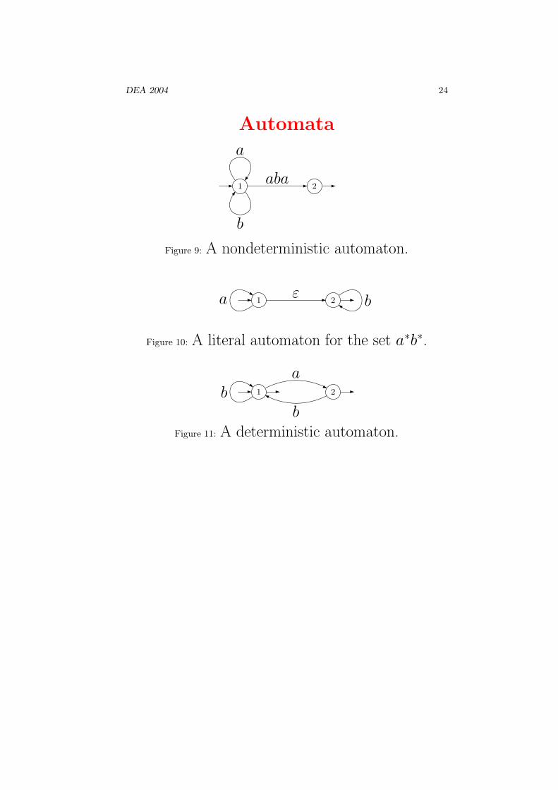
Automata

1 2

b

a

aba

Figure 9: A nondeterministic automaton.

1 2a bε

Figure 10: A literal automaton for the set a∗b∗.

1 2ba

bFigure 11: A deterministic automaton.

DEA 2004 25

The classes NFA and DFA

The class NFA implements nondeterministic finite

automata. The states are represented by integers

and the transitions by sets of half-edges, i.e. of

pairs (s, q) of a word and a state. The half-

edges are objects of the class HalfEdge. A set

of half-edges is represented as a Set (actually a

TreeSet from the Java API ). The set of initial

and the set of terminal states are also represented

by a Set. The alphabet is given as an object of

the class Alphabet.

The class DFA implements deterministic com-

plete finite automata. The alphabet is an object

of the class Alphabet. The transition function is

represented by a double array next[][]. The set

of terminal states is given by a partition of the set

of states (class Partition). A state q is terminal

if terminal.blockName[p]=1 (the default value

is 0).

DEA 2004 26

The classes INFA and IDFA

The class INFA implements incomplete nondeter-

ministic finite automata (without epsilon transi-

tions). The edges going out of a state are imple-

mented in a Queue (class PairIntQueue). The

automaton itself is an array of Queues.

This class implements incomplete deterministic

automata. The edges going out of a state are im-

plemented in a Queue (class PairIntQueue). The

automaton itself is an array of Queues. The space

used by this implementation is O(n + k + e) for a

deterministic automaton on k letters, n states and

e edges, instead of O(kn) for the class DFA. This

representation is preferable when k is large.

DEA 2004 27

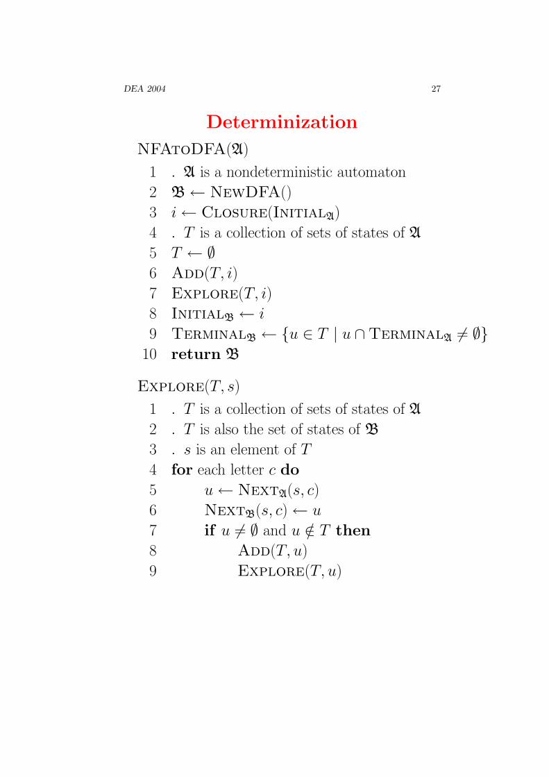
Determinization

NFAtoDFA(A)

1 . A is a nondeterministic automaton

2 B← NewDFA()

3 i← Closure(InitialA)

4 . T is a collection of sets of states of A

5 T ← ∅6 Add(T, i)

7 Explore(T, i)

8 InitialB ← i

9 TerminalB ← {u ∈ T | u ∩TerminalA 6= ∅}10 return B

Explore(T, s)

1 . T is a collection of sets of states of A

2 . T is also the set of states of B

3 . s is an element of T

4 for each letter c do

5 u← NextA(s, c)

6 NextB(s, c)← u

7 if u 6= ∅ and u /∈ T then

8 Add(T, u)

9 Explore(T, u)

DEA 2004 28

Examples

First example: Second example:

1 2bb

a

Figure 12: The nondeterministic automaton A.

1, 2 1ba

bFigure 13: The deterministic version B of A.

1, 2 2a bb

Figure 14: A deterministic automaton for the set a∗b∗.

DEA 2004 29

Gilbreath’s trick

Consider a deck of 2n cards ordered in such a

way that red and black cards alternate. Cut

the deck into two parts and give it a riffle shuf-

fle. Cut it once more, this time not completely

arbitrarily but at a place where two cards of

the same colour meet. Square up the deck.

Then for every i = 1, . . . , n the pair consisting

of the (2i − 1)-th and the 2i-th card is of the

form (red, black) or (black, red).

Translation:

F ((ab)∗) tt F ((ab)∗) = F ((ab + ba)∗) .

1 2 3

b

a

a

b

123

12

23

1

3

2

a

b

a

ba

a

b

a

b

a

Figure 15: A deterministic automaton recognizing the

set F ((ab + ba)∗).

DEA 2004 30

1 2

a

b

1, 1 1, 2

2, 1 2, 2

a

a

ab

ab

b

b

Figure 16: Two automata, recognizing F ((ab)∗) and

F ((ab)∗) tt F ((ab)∗).

1 2

3 4

a

a

a

b

a

b

b

b 1234

234

123

4

1

23

a

b

a

ba

a

b

a

b

a

Figure 17: A deterministic automaton recognizing the

set F ((ab)∗) tt F ((ab)∗).

DEA 2004 31

Minimization of automata

0 1 2 . . . n n + 1

a, b

a a, b a, b

Figure 18: Recognizing the words with an a at the

n + 1-th position before the end

DEA 2004 32

Moore’s algorithm

Minimization()

1 f ← InitialPartition()

2 do e← f

3 . e is the old partition, f is the new one

4 f ← Refine(f)

5 while e 6= f

6 return e

Refine(e)

1 for a ∈ A do

2 g ← a−1e

3 e← Intersection(e, g)

4 return e

Complexity: O(n2k for n states and k letters.

DEA 2004 33

Example

12 3

b

ca, c

a

b

1 13

2 12

ca

ac

ba

cb

bc

Figure 19: Recognizing the set (a + bc + ab + c)∗

1 3

2 4

ca

ac

ba

cb

bc 12 3

b

cc a

a

b, c

Figure 20: The minimization algorithm

DEA 2004 34

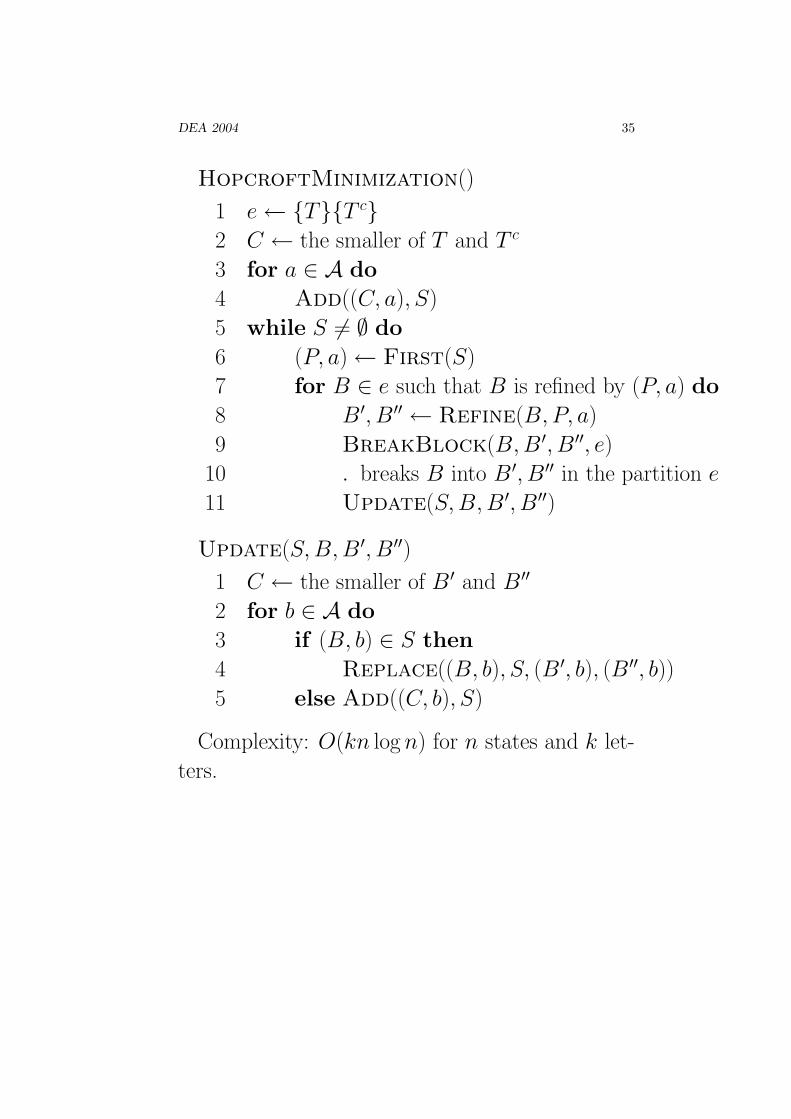
Hopcroft’s algorithm

The algorithm starts with the partition composed

of the set T of terminal states and its complement

T c. It maintains a set S of pairs (P, a) formed of

a set of states and a letter.

The main loop consists in selecting a pair (P, a)

from the set S. Then for each block B of the

current partition which is refined by (P, a) into

B′, B′′, one performs the following steps

1. replace B by B′ and B′′ in the current parti-

tion,

2. for each letter b,

(a) if (B, b) is in S, then replace (B, b) by (B ′, b)and (B′′, b) in S,

(b) otherwise add to S the pair (C, b) where C

is the smaller of the sets B ′ and B′′.

DEA 2004 35

HopcroftMinimization()

1 e← {T}{T c}2 C ← the smaller of T and T c

3 for a ∈ A do

4 Add((C, a), S)

5 while S 6= ∅ do

6 (P, a)← First(S)

7 for B ∈ e such that B is refined by (P, a) do

8 B′, B′′ ← Refine(B, P, a)

9 BreakBlock(B, B ′, B′′, e)10 . breaks B into B ′, B′′ in the partition e

11 Update(S, B, B′, B′′)

Update(S, B, B′, B′′)

1 C ← the smaller of B ′ and B′′

2 for b ∈ A do

3 if (B, b) ∈ S then

4 Replace((B, b), S, (B ′, b), (B′′, b))5 else Add((C, b), S)

Complexity: O(kn log n) for n states and k let-

ters.

DEA 2004 36

0 1 2 3 4 5

class 1 2 0 2 0 2

0 1 2

card 2 1 3

(a) The classesand their size

0 1 2

block

0 1 2 3 4 5

location

2

4

0 1

3

5

(b) The blocks ofthe partition

Figure 21: A partition of Q = {0, . . . , 5}. The class

of a state is the integer in the array class. The

size of a class is given in the array card. The

elements of a block are chained in a doubly linked

list pointed to by the entry in the array block.

Each cell in these lists can be retrieved in constant

time by its state using the pointer in the array

location.

DEA 2004 37

Revuz algorithm

To be used only with acyclic automata.

AcyclicMinimization()

1 . ν[p] is the state corresponding to p in the minimal automaton

2 (Q0, . . . , QH)← PartitionByHeight(Q)

3 for p in Q0 do

4 ν[p]← 0

5 k ← 0

6 for h← 1 to H do

7 S ← Signatures(Qh, ν)

8 P ← RadixSort(Qh, S) . P is the sorted sequence Qh

9 p← first state in P

10 ν[p]← k

11 k ← k + 1

12 for each q in P \ p in increasing order do

13 if σ(q) = σ(p) then

14 ν[q]← ν[p]

15 else ν[q]← k

16 (k, p)← (k + 1, q)

17 return ν

Complexity: O(n+ k) on n states and k letters.

DEA 2004 38

The class MinAutomaton

This class implements a command computing the

minimal automaton of a set of words given in a

text file using one of several possible minimization

algorithms. The minimization algorithms are con-

tained in the classes implementing the Minimizer

interface. Usage:

java MinAutomaton method file (option)

The method can be

• N (naive method using NMinimizer)

• Nbis (a variant of the previous using NbisMinimizer)

• H (Hopcroft’s algorithm using HopcroftMinimizer)

• R (Revuz algorithm using RMinimizer to be

used only with acyclic automata represented as

IDFA.

The option can be v (verbose mode).

DEA 2004 39

The interface Minimizer

This interface is implemented by the classes

• BMinimizer implementing the Brzozowski min-

imization algorithm.

• HopcroftMinimizer implementing the Hopcroft

minimization algorithm.

• FMinimizer implementing the fusion minimiza-

tion algorithm.

• NMinimizer implementing the naive minimiza-

tion algorithm.

• RMinimizer implementing the Revuz minimiza-

tion algorithm.

DEA 2004 40

Pattern Matching

• Thomson’s construction

• The class LinkedNFA

• The class CompileExpression

DEA 2004 41

Thomson’s construction

ε a

Figure 22: Automata for the empty set, for ε and for

a

Figure 23: Automata for union, product and star.

DEA 2004 42

BuildAutomaton(a)

1 A← NewAutomaton()

2 Next1(InitialA)← (a,TerminalA)

3 return A

AutomataUnion(A, B)

1 C← NewAutomaton()

2 Next1(InitialC)← (ε, InitialA)

3 Next2(InitialC)← (ε, InitialB)

4 Next1(TerminalA)← (ε,TerminalC)

5 Next1(TerminalB)← (ε,TerminalC)

6 return C

AutomataProduct(A, B)

1 C← NewAutomaton()

2 InitialC ← InitialA

3 TerminalC ← TerminalB

4 Merge(TerminalA, InitialB)

5 return C

DEA 2004 43

AutomatonStar(A)

1 B← NewAutomaton()

2 Next1(InitialB)← (ε, InitialA)

3 Next2(InitialB)← (ε,TerminalB)

4 Next1(TerminalA)← (ε, InitialA)

5 Next1(TerminalA)← (ε,TerminalB)

6 return C

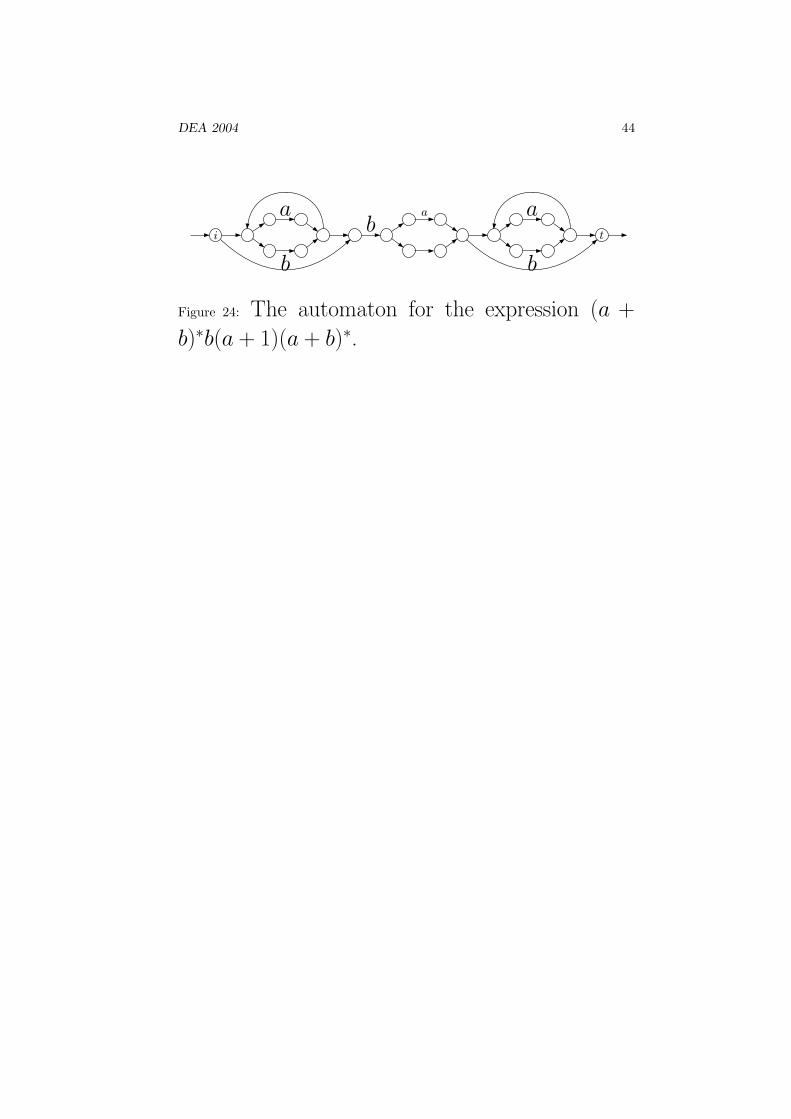
DEA 2004 44

i t

a

b

ba a

b

Figure 24: The automaton for the expression (a +

b)∗b(a + 1)(a + b)∗.

DEA 2004 45

The class LinkedNFA

Implementation of automata by linked lists in view

of Thomson’s algorithm. The states of automata

are objects of the class State. Each state has

two pointers to its successors. The choice of this

representation allows easily the implementation of

the operations of union, product and star on au-

tomata. The automata have the properties that

there are at most two edges going out of a state,

there is only one initial state, only one terminal

state, no edge comes into the initial state, no edge

goes out of the terminal state.

DEA 2004 46

The class CompileExpression

Compiles a regular expression into a finite automa-

ton by one of the possible methods implementing

the interface ExpressionCompiler Usage:

java CompileExpression Method Option expression

The only method presently available is T (Thom-

son’s algorithm using ThompsonCompiler). The

options available are:

• N to produce an NFA

• D to produce a DFA

• M to produce the minimal automaton.

For example, the command

java CompileExpression T M "(ab+ba)*"

produces

Thompson’s algorithm

alphabet:ab

Minimal automaton

initial=0

nbStates=4

0 1 3

1 2 0

2 2 2

3 0 2

DEA 2004 47

terminals = 0 .

DEA 2004 48

Transducers

• Transducers

• Examples

• Composition

• Determinization

• Minimization

• The classes NFT and DFT

DEA 2004 49

Transducers

input

q

output

Figure 25: A transducer reads the input and writes the

output.

DEA 2004 50

Examples

0a | ab b | a 0b | a 1

a | a

ε | bFigure 26: The Fibonacci morphism.

0 1a | a b | bb | a

a | b0 1a | a b | b

a | b

b | a

Figure 27: The circular right shift on words ending

with a and its inverse.

DEA 2004 51

Composition

0, 0

1, 0

1, 1

0, 1

a | a

b | a b | a

b | b

a | ba | b

b | b a | a

Figure 28: The right 2-shift.

ComposeTransducers(S, T)

1 . S and T are literal transducers

2 U← NewTransducer()

3 for each edge (p, a, b, q) of S do

4 for each edge (r, b, c, s) of T do

5 add ((p, r), a, c, (q, s)) to the edges of U

6 for each edge (p, a, ε, q) of S do

7 for each state r of T do

8 add ((p, r), a, ε, (q, r)) to the edges of U

9 for each edge (r, ε, c, s) of T do

10 for each state p of S do

11 add ((p, r), ε, c, (p, s)) to the edges of U

12 InitialU ← InitialS × InitialT

13 TerminalU ← TerminalS ×TerminalT

14 return U

DEA 2004 52

0 1ε | a

2ε | b

0, 0 1, 1ε | a

1, 0ε | b

2, 0ε | a

Figure 29: The image f(x) = aba of x = ab by the

Fibonacci morphism.

DEA 2004 53

Sequential transducers

A sequential transducer over A, B is a triple

(Q, i, T ) together with a partial function

Q×A → B∗ ×Q

which breaks up into a next state function Q ×A → Q and an output function Q×A → B∗. As

usual, the next state function is denoted (q, a) 7→q · a and the output function (q, a) 7→ q ∗ a. In

addition, the initial state i ∈ Q has attached a

word λ called the initial prefix and T is actually a

(partial) function T : Q→ B∗ called the terminal

function .

0 1a | ε a

a | a

b | b

Figure 30: A sequential transducer for the circular left

shift on words beginning with a.

DEA 2004 54

Determinization of transducers

ToSequentialTransducer(A)

1 . A is a transducer

2 B← NewSequentialTransducer()

3 I ← Closure({ε} × InitialA)

4 InitialB ← I

5 . T is a collection of sets of half-edges

6 T ← I

7 (T , B)← Explore(T , I, B)

8 for S ∈ T do

9 for (u, q) ∈ S do

10 if q ∈ TerminalA then

11 TerminalB(S)← u

12 return B

Explore(T , S, B)

1 . T is a collection of sets of half-edges

2 . S is an element of T3 for each letter a do

4 (v, U)← Lcp(Next(S, a))

5 NextB(S, a)← (v, U)

6 if U 6= ∅ and U /∈ T then

7 T ← T ∪ U

8 (T , B)← Explore(T , U, B)

9 return (T , B)

DEA 2004 55

Examples

ε,0a,0b,1

a | ε a

a | a

b | b

Figure 31: A sequential transducer for the circular left

shift on words beginning with a obtained by the

determinization algorithm.

DEA 2004 56

Minimization of transducers

The normalized transducer is obtained by modify-

ing the output function and terminal function of

A. We set

λ′ = λπi , p∗′a = π−1

p (p∗a)πp.a , T ′(p) = π−1

p T (p)

0b | a 1

a | aa | ba

b | ba

b0b | a 1

a | aba | ab

b | a

Figure 32: The normalization algorithm.

DEA 2004 57

LongestCommonPrefixArray(A)

1 . P, P ′ are arrays of strings initially null

2 . M is the matrix of transitions of A and N the vector of terminals

3 do P ← P ′

4 P ′ ← MP + N

5 while P 6= P ′

6 return P

NormalizeTransducer(A)

1 P ← LongestCommonPrefixArray(A)

2 (λ, i)← Initial

3 Initial← (λP [i], i)

4 for (p, a) ∈ Q× A do

5 (u, q)← Next(p, a)

6 Next(p, a)← P [p]−1uP [q]

7 for p ∈ Q do

8 T [p]← P [p]−1T [p]

DEA 2004 58

Example

0b | a 1

a | aba | ab

b | a0b | a a | ab

Figure 33: The minimization algorithm.

DEA 2004 59

The classes NFT and DFT

The class NFT implements nondeterministic finite-

state transducers (NFT). It extends the class NFA.The

states are represented by integers and the tran-

sitions by an array of sets of ternary half-edges,

i.e. triples (s, t, q) of an input word, an out-

put word and a state (class HalfEdge). A set of

half edges is represented by a TreeSet. The sets

of initial and terminal states are represented by

TreeSet objects. The alphabet is given as an ob-

ject of the class Alphabet.

The class DFT implements sequential (or deter-

ministic) finite-state transducers. These inherit

from deterministic finite-state automata (class DFA)

adding an output function, an initial output (as-

sociated with the initial state) and a terminal out-

put function. The terminal states are those with a

nonempty output.

DEA 2004 60

Parsing

• Grammars

• The class Grammar

• Top-down analysis

• First and Follow

• The class LL

• Bottom-up analysis

• The class SLR

DEA 2004 61

Grammars

The Dyck language is generated by the grammar

G with sets A = {a, b},V = {v} and the produc-

tions

v → avbv, v → ε.

v

a v

ε

b v

a v

a v

ε

b v

ε

b v

ε

Figure 34: A derivation tree for the word abaabb in the

Dyck grammar.

DEA 2004 62

The class Grammar

This class implements context-free grammars. The

productions of the grammar are stored in an array

productionsArray. Each production is an ob-

ject of the class Production. There are separated

alphabets terminals for terminals and variables

for variables plus an alphabet alphabet for their

union. The usual functions First() and Follow()

are implemented as methods of this class. The

grammar can be read from a file where the pro-

ductions are listed one by line in the form l:r

with a ”:” separating the two sides of each produc-

tion. The initial rule should be the last one. The

following grammars are included in the directory

Data:

ETF.txt the ordinary ETF grammar, which is

SLR but not LL(1).

ETFPrime.txt the variant of the ETF grammar

which is LL(1) obtained by eliminating left recur-

sion.

Dyck.txt the grammar of the Dyck language, which

is LL(1).

DEA 2004 63

Top-down parsing

The idea of top-down parsing is to build the deriva-

tion tree from the rooti

@@

@@

@@

@@

��

��

��

��

w

��

��y zx

Figure 35: Top down parsing.

E → E + T | TT → T ∗ F | FF → (E) | c

DEA 2004 64

EvalExp()

1 v ← EvalTerm()

2 while Current() = ‘+’ do

3 Advance()

4 v ← v + EvalTerm()

5 return v

EvalTerm()

1 v ← EvalFact()

2 while Current() = ‘∗’ do

3 Advance()

4 v ← v ∗ EvalFact()

5 return v

EvalFact()

1 if Current() = ‘(’ then

2 Advance()

3 v ← EvalExp()

4 Advance()

5 else v ← Current()

6 Advance()

7 return v

DEA 2004 65

First and Follow

The precise definition of LL(1) grammars uses two

functions called First() and Follow() that as-

sociate to each variable a set of terminal symbols.

For a variable x ∈ V , First(x) is the set of termi-

nal symbols a ∈ A such that there is a derivation

of the form x∗→ au. The function First() is

extended to words in a natural way: First(w) is

the set of terminal symbols a such that w∗→ au.

For each variable x ∈ V , Follow(x) is the set

of terminal symbols a ∈ A such that there is a

derivation u∗→ vxaw with a “following” x.

E T F

(

c

(a) First().

E

) + $

T F

(b) Follow().

Figure 36: The graphs of First() and of Follow().

DEA 2004 66

Epsilon()

1 for each production v → ε do

2 epsilon[v]← true

3 for i← 0 to n− 1 do

4 for each production v → x1 · · ·xm do

5 epsilon[v]← epsilon[v] ∨ (epsilon[x1] ∧ · · · ∧ epsilon[xm])

6 return epsilon

FirstChild(v)

1 . S is the set of successors of v

2 S ← ∅3 for each production v → x1 · · ·xm do

4 for i← 1 to m do

5 S ← S ∪ xi

6 if epsilon[xi] = false then

7 break

8 return S

ExploreFirstChild(v)

1 firstmark[v]← true

2 for each x ∈ FirstChild(v) do

3 if firstmark[x] = false then

4 ExploreFirstChild(x)

DEA 2004 67

First(v)

1 . mark is an array initialized to false

2 ExploreFirstChild(v)

3 S ← ∅4 for each terminal c do

5 if firstmark[c] then

6 S ← S ∪ c

7 return S

First(w)

1 S ← ∅2 for i← 1 to n do . w has length n

3 S ← S ∪ First(w[i])

4 if epsilon[w[i]] = false then

5 break

6 return S

To compute the function Follow(), we build

a similar graph. There are two rules to define the

edges.

1. if there is a production x → uvw with a ter-

minal symbol a in First(w), then (v, a) is an

edge.

2. if there is a production z → uxw with w∗→ ε,

then (x, z) is an edge (notice that we use the

DEA 2004 68

productions backwards).

Sibling(x)

1 S ← ∅2 for each production z → uxw do

3 S ← S ∪ First(w)

4 if IsNullable(w) then

5 S ← S ∪ z

6 return S

Follow(v)

1 . followmark is an array initialized to false

2 ExploreSibling(v)

3 S ← ∅4 for each terminal c do

5 if followmark[c] then

6 S ← S ∪ c

7 return S

DEA 2004 69

LLTable()

1 . computes the LL(1) parsing table M

2 for each production p : v → w do

3 for each terminal c ∈ First(w) do

4 M [v][c]← p

5 if w = ε then

6 for each terminal c ∈ Follow(v) do

7 M [v][c]← p

8 return M

DEA 2004 70

The class LL

Implements the LL(1) top-down analysis. Usage:

java LL "input" grammar.

The normal execution shows the evolution of the

stack ended by the message ”input accepted”. If

the grammar is not LL(1), an error message is is-

sued. The message also indicates which rules gen-

erate the conflict. If the input is not correct, an

error message Syntax error or Syntax error:

end of input is issued. For example, the com-

mand

java LL "(1+2)*3" ../Data/ETFPrime.txt

produces

LL table

$ ( ) * + c

E - 0 - - - 0

F - 6 - - - 7

I - 8 - - - 8

T - 3 - - - 3

e 2 - 2 - 1 -

t 5 - 5 4 5 -

alphabet

$()*+EFITcet

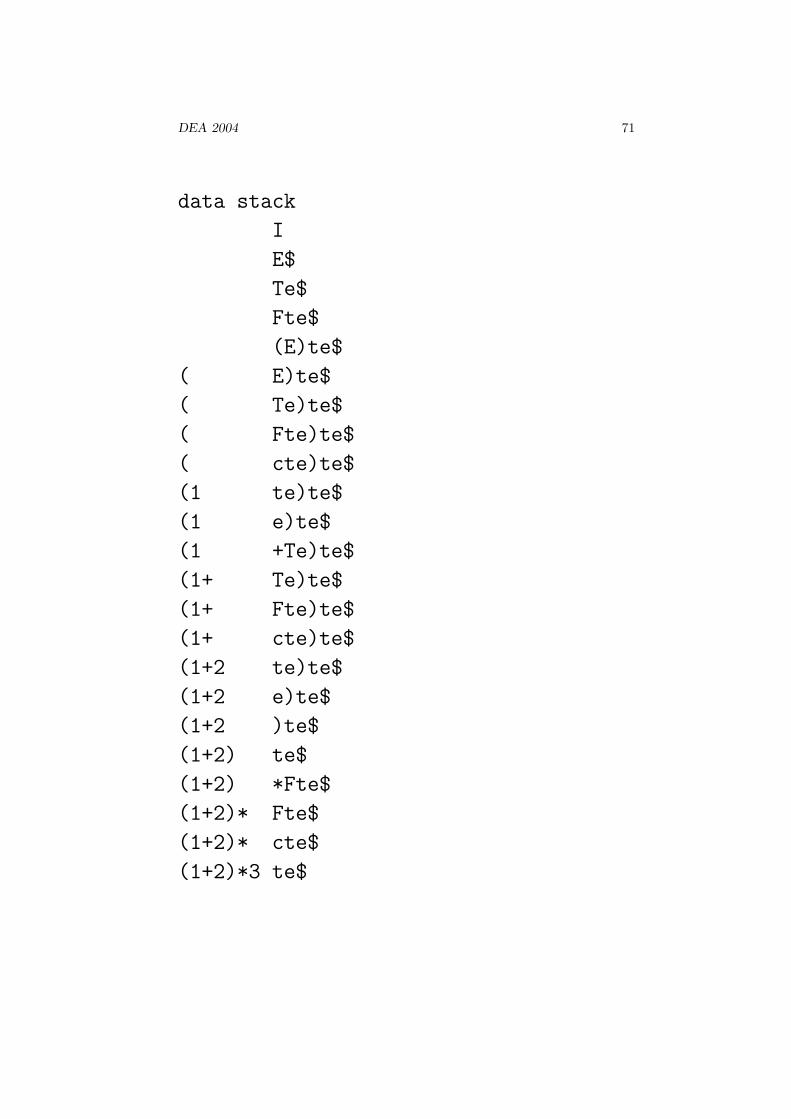
DEA 2004 71

data stack

I

E$

Te$

Fte$

(E)te$

( E)te$

( Te)te$

( Fte)te$

( cte)te$

(1 te)te$

(1 e)te$

(1 +Te)te$

(1+ Te)te$

(1+ Fte)te$

(1+ cte)te$

(1+2 te)te$

(1+2 e)te$

(1+2 )te$

(1+2) te$

(1+2) *Fte$

(1+2)* Fte$

(1+2)* cte$

(1+2)*3 te$

DEA 2004 72

(1+2)*3 e$

(1+2)*3 $

(1+2)*3$

input accepted

whereas the command

java LL "(1+2)*3" ../Data/ETF.txt

produces

Conflict between rules 1 and 0

java.lang.Exception: The grammar is not

LL(1)

and the command

java LL "(1+2)3" ../ETFPrime.txt

produces

java.lang.Exception: Syntax error

DEA 2004 73

Bottom-up parsing

The idea of bottom-up parsing is to build the deriva-

tion tree from the leaves to the root.i

@@

@@

@@

@@

��

��

��

��

stack�

���

textx

Figure 37: Bottom up parsing.

1 : E → E + T

2 : E → T

3 : T → T ∗ F

4 : T → F

5 : F → (E)

6 : F → c

There are two kinds of actions performed by the

DEA 2004 74

Stack Text(1 + 2) ∗ 3

( 1 + 2) ∗ 3(c +2) ∗ 3(F +2) ∗ 3(T +2) ∗ 3(E +2) ∗ 3(E+ 2) ∗ 3(E + c ) ∗ 3(E + F ) ∗ 3(E + T ) ∗ 3(E ) ∗ 3(E) ∗3F ∗3T ∗3T∗ 3T ∗ c

T ∗ F

T

E

Figure 38: Evolution of the stack and of the text during

the bottom-up analysis of the expression (1+2)∗3.

DEA 2004 75

0 1E

6+

9T

to 9∗

to 3F

to 4(

to 5c

2T

7∗

10F

to 4(

to 5c

3F

4(

(

8E

11)

to 6+

to 2T

to 3F

5c

c

Figure 39: The LR automaton.

DEA 2004 76

Stack Text0 (1 + 2) ∗ 3$0 4 1 + 2) ∗ 3$0 4 5 +2) ∗ 3$0 4 3 +2) ∗ 3$0 4 2 +2) ∗ 3$0 4 8 +2) ∗ 3$0 4 8 6 2) ∗ 3$0 4 8 6 5 ) ∗ 3$0 4 8 6 3 ) ∗ 3$0 4 8 6 9 ) ∗ 3$0 4 8 ) ∗ 3$0 4 8 11 ∗3$0 3 ∗3$0 2 ∗3$0 2 7 3$0 2 7 5 $0 2 7 10 $0 2 $0 1 $

Figure 40: The stack of states of the LR automaton

during the bottom-up analysis of the expression

(1 + 2) ∗ 3.

analyser:

• shift a symbol from the data to the stack. Ac-

tually it is the state of the LR automaton which

is pushed on the stack instead of the symbol.

• reduce the stack using a production v → w of

the grammar. This is done in two steps: first

pop |w| symbols from the stack, then push v

(i.e. the corresponding LR state).

For each pair (lookahead symbol, state on top of

DEA 2004 77

c + ∗ ( ) $ E T F

0 5 4 1 2 31 6 Acc

2 734 5 4 8 2 356 5 4 9 37 5 4 108 6 119 71011

c + ∗ ( ) $ E T F

012 2 2 23 4 4 4 445 6 6 6 66789 1 1 110 3 3 3 311 5 5 5 5

Figure 41: The arrays S and R

the stack) the arrays S (for shift) and R (for re-

duce) store the information needed:

• state to be pushed

• rule to be used

DEA 2004 78

LRParse(x)

1 while Top() 6= Accept do

2 p← Top()

3 c← Current()

4 q ← T [p][c]

5 if q 6= −1 then

6 Push(q)

7 Advance()

8 else n← R[p][c]

9 if n 6= −1 then

10 Reduce(n)

11 else return false

12 return true

DEA 2004 79

0 1E

2+

3T

to 6, 10

4 5T

to 6, 10

6 7T

8∗

9F

to 12, 16

10 11F

to 12, 16

12 13(

14E

15)

to 0, 4

16 17c

Figure 42: A non deterministic LR automaton

DEA 2004 80

The class SLR

This class implements the SLR(0) method for syn-

tax analysis. Usage:

java SLR "input" grammar

For instance,

java SLR "(1+2)*3" ../Data/ETF.txt

produces the successive stack contents during the

analysis of the expression (1+2)*3 using the ETF

grammar. If the grammar is not SLR, an error mes-

sage Grammar not SLR: S/R conflict is issued.

If the expression is not correct, an error message

syntax error or end of input reached is is-

sued.

The construction of the LR(0) automaton is per-

formed by the method LRAutomaton. It is imple-

mented as a variant of an ordinary NFA called an

InfoNFA. Each state carries an additional infor-

mation stored in the array info[] which is the

index of the rule by which there is a possible reduc-

tion. This information is passed through the deter-

minization algorithm to the states of the InfoDFA.

DEA 2004 81

Word enumeration

Example 1: The number un of words of length n

on the binary alphabet {a, b} which do not contain

two consecutive a’s satisfies the recurrence formula

un+1 = un + un−1. From the automaton:

S1 = S1b + S2b + ε

S2 = S1a

Since u0 = 1 and u1 = 2, the number un is the

Fibonacci number Fn+2.

Example 2: The Dyck language D∗ satisfies the

relationD = aD∗b. Let fn be the number of words

of length n in D. This implies that the generating

function D(z) =∑

n≥0fnz

n satisfies the equation

D2 −D + z2 = 0 .

It follows that

D(z) =1−√

1− 4z2

2.

An elementary application of the binomial formula

gives

f2n =1

n

(

2n− 2

n− 1

)

.

DEA 2004 82

The Perron-Frobenius Theorem

The Perron–Frobenius Theorem asserts that for

any nonnegative matrix M , the following holds

1. The matrix M has a real eigenvalue ρM such

that |λ| ≤ ρM for any eigenvalue λ of M .

2. If M ≤ N with M 6= N , then ρM < ρN .

3. There corresponds to ρM a nonnegative eigen-

vector v and ρM is the only eigenvalue with a

nonnegative eigenvector.

4. If M is irreducible, the eigenvalue ρM is simple

and there corresponds to ρM a positive eigen-

vector v.

5. If M is primitive, all other eigenvalues have

modulus strictly less than ρM . Moreover, 1

ρnM

Mn

converges to a matrix of the form vw, where v

(w) is a right (left) eigenvector corresponding

to ρ, i.e. Mv = ρv (wM = ρw) and wv = 1.

DEA 2004 83

DominantEigenvalue(M, x)

1 y ← x

2 do (y, x)← (Mx, y)

3 r ← min1≤i≤n yi/xi

4 y ← 1

ry

5 while y 6≈ x

6 return r

DEA 2004 84

Probability distributions onwords

• Entropy

• Ziv-Lempel compression

DEA 2004 85

Entropy

Entropy(n)

1 . returns the n-th order entropy Hn

2 S ← ∅ . S is the set of n-grams in the text

3 do s← Current() . s is the current n-gram of the text

4 if s /∈ S then

5 S ← S ∪ s

6 Freq(s)← 1

7 else Freq(s)← Freq(s) + 1

8 while there are more symbols

9 for s ∈ S do

10 Prob(s)← Freq(s)/Card S

11 return1

n

∑

s∈SProb(s) log Prob(s)

DEA 2004 86

Ziv-Lempel compression

ZLencoding(w)

1 . returns the Ziv–Lempel encoding c of w

2 T ← NewTrie()

3 (c, i)← (ε, 0)

4 while i < |w| do

5 (`, p)← LongestPrefixInTrie(w, i)

6 a← w[i + `]

7 q ← NewVertex()

8 Next(p, a)← q . updates the trie T

9 c← c · (p, a) . appends (p, a) to c

10 i← i + ` + 1

11 return c

ZLdecoding(c)

1 (w, i)← (ε, 0)

2 D[i]← ε

3 while c 6= ε do

4 (p, a)← Current() . returns the current pair in c

5 Advance()

6 y ← D[p]

7 i← i + 1

8 D[i]← ya . adds ya to the dictionary

9 w ← wya

10 return w