Embed Size (px)
Citation preview

ROBERT SEDGEWICK | KEVIN WAYNE
F O U R T H E D I T I O N
Algorithms
http://algs4.cs.princeton.edu
Algorithms ROBERT SEDGEWICK | KEVIN WAYNE
LINEAR PROGRAMMING
‣ brewer’s problem
‣ simplex algorithm
‣ implementations
‣ reductions
2
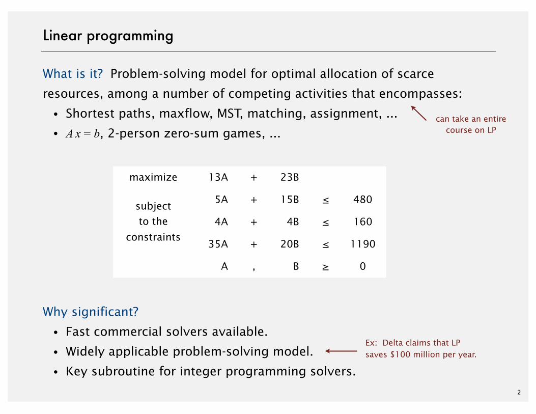
Linear programming
What is it? Problem-solving model for optimal allocation of scarce
resources, among a number of competing activities that encompasses:
・Shortest paths, maxflow, MST, matching, assignment, ...
・A x = b, 2-person zero-sum games, ...
Why significant?
・Fast commercial solvers available.
・Widely applicable problem-solving model.
・Key subroutine for integer programming solvers.
Ex: Delta claims that LPsaves $100 million per year.
maximize 13A + 23B
subjectto the
constraints
5A + 15B ≤ 480subjectto the
constraints 4A + 4B ≤ 160
subjectto the
constraints35A + 20B ≤ 1190
A , B ≥ 0
can take an entirecourse on LP
3
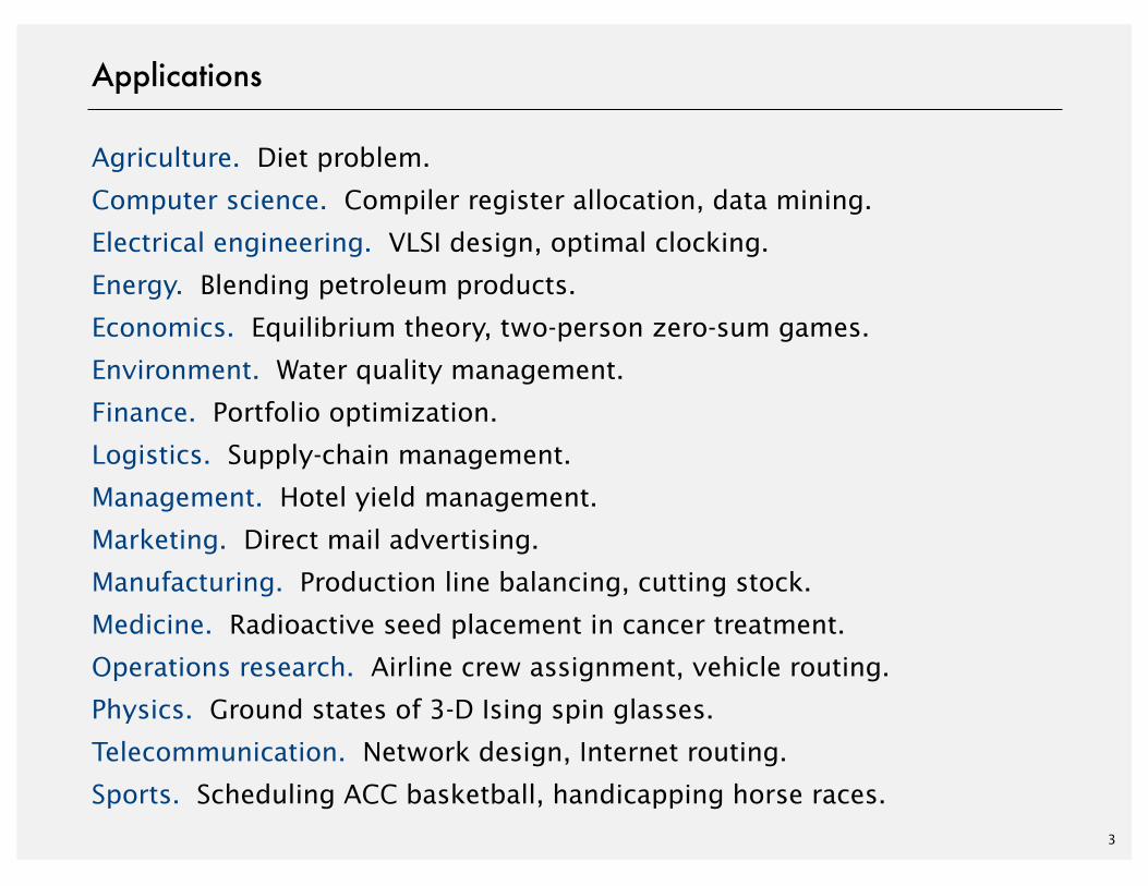
Applications
Agriculture. Diet problem.
Computer science. Compiler register allocation, data mining.
Electrical engineering. VLSI design, optimal clocking.
Energy. Blending petroleum products.
Economics. Equilibrium theory, two-person zero-sum games.
Environment. Water quality management.
Finance. Portfolio optimization.
Logistics. Supply-chain management.
Management. Hotel yield management.
Marketing. Direct mail advertising.
Manufacturing. Production line balancing, cutting stock.
Medicine. Radioactive seed placement in cancer treatment.
Operations research. Airline crew assignment, vehicle routing.
Physics. Ground states of 3-D Ising spin glasses.
Telecommunication. Network design, Internet routing.
Sports. Scheduling ACC basketball, handicapping horse races.
http://algs4.cs.princeton.edu
ROBERT SEDGEWICK | KEVIN WAYNE
Algorithms
‣ brewer’s problem
‣ simplex algorithm
‣ implementations
‣ reductions
Allocation of Resources by Linear Programmingby Robert Bland
Scientific American, Vol. 244, No. 6, June 1981
LINEAR PROGRAMMING
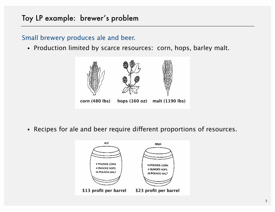
Small brewery produces ale and beer.
・Production limited by scarce resources: corn, hops, barley malt.
・Recipes for ale and beer require different proportions of resources.
5
Toy LP example: brewer’s problem
$13 profit per barrel $23 profit per barrel
corn (480 lbs) hops (160 oz) malt (1190 lbs)
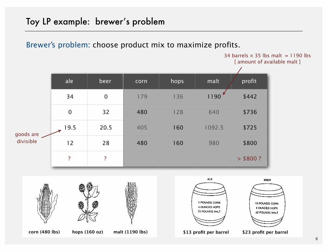
Brewer’s problem: choose product mix to maximize profits.
ale beer corn hops malt profit
34 0 179 136 1190 $442
0 32 480 128 640 $736
19.5 20.5 405 160 1092.5 $725
12 28 480 160 980 $800
? ? > $800 ?
6
Toy LP example: brewer’s problem
34 barrels × 35 lbs malt = 1190 lbs[ amount of available malt ]
corn (480 lbs) hops (160 oz) malt (1190 lbs) $13 profit per barrel $23 profit per barrel
goods aredivisible
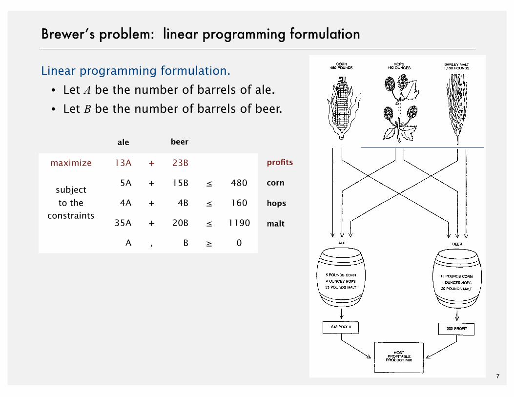
Linear programming formulation.
・Let A be the number of barrels of ale.
・Let B be the number of barrels of beer.
7
Brewer’s problem: linear programming formulation
maximize 13A + 23B
subjectto the
constraints
5A + 15B ≤ 480subjectto the
constraints 4A + 4B ≤ 160
subjectto the
constraints35A + 20B ≤ 1190
A , B ≥ 0
ale beer
corn
hops
malt
profits
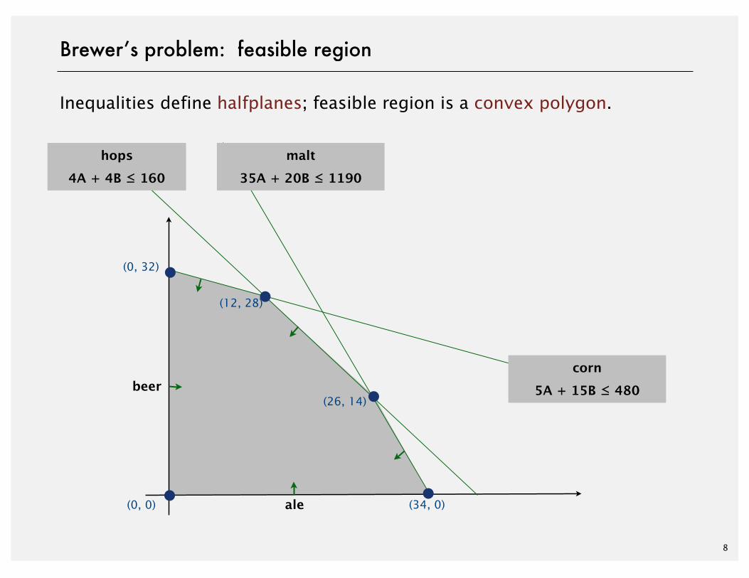
Inequalities define halfplanes; feasible region is a convex polygon.
8
Brewer’s problem: feasible region
(34, 0)
(0, 32)
(12, 28)
(26, 14)
(0, 0) ale
beercorn
5A + 15B ≤ 480
hops4A + 4B ≤ 160
malt35A + 20B ≤ 1190
(34, 0)
(0, 32)
(12, 28)
(26, 14)
(0, 0)
9
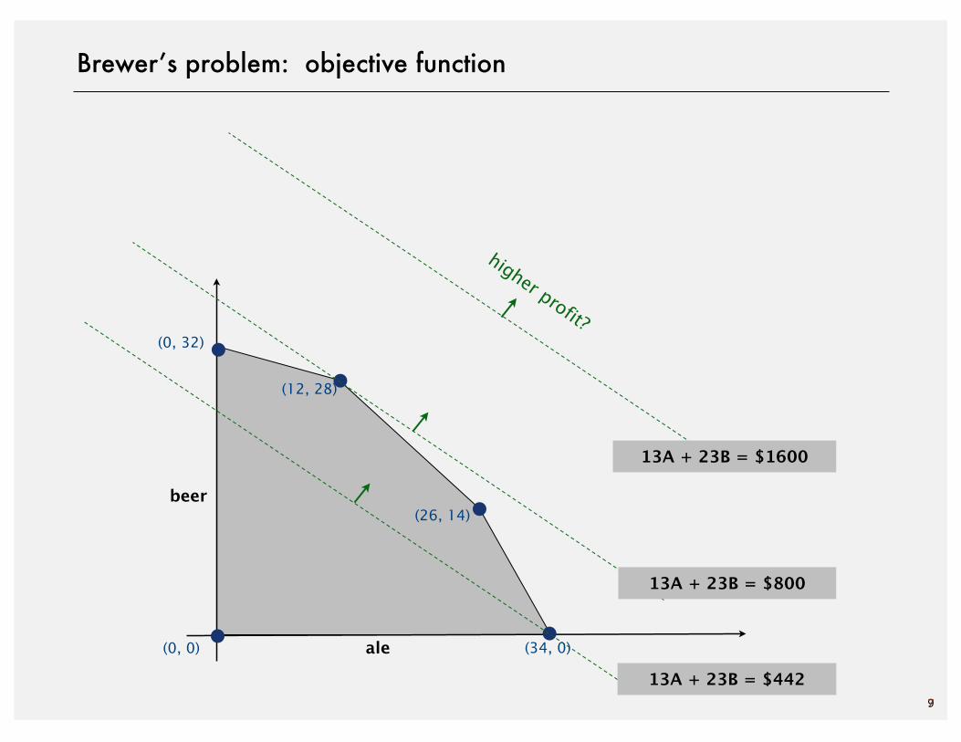
Brewer’s problem: objective function
higher profit?
7
ale
beer
13A + 23B = $800
13A + 23B = $1600
13A + 23B = $442
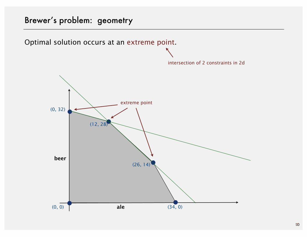
Optimal solution occurs at an extreme point.
(34, 0)
(0, 32)
(12, 28)
(26, 14)
(0, 0)
10
Brewer’s problem: geometry
extreme point
7
ale
beer
intersection of 2 constraints in 2d
11
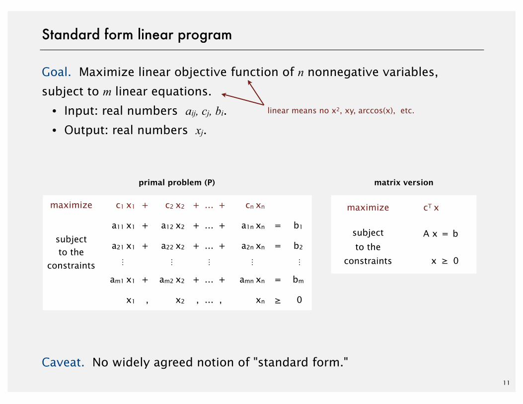
Standard form linear program
Goal. Maximize linear objective function of n nonnegative variables,
subject to m linear equations.
・Input: real numbers aij, cj, bi.
・Output: real numbers xj.
Caveat. No widely agreed notion of "standard form."
maximize cT x
subject
to the constraints
A x = bsubject
to the constraints x ≥ 0
matrix versionprimal problem (P)
linear means no x2, xy, arccos(x), etc.
maximize c1 x1 + c2 x2 + … + cn xn
subjectto the
constraints
a11 x1 + a12 x2 + … + a1n xn = b1
subjectto the
constraints
a21 x1 + a22 x2 + … + a2n xn = b2subjectto the
constraints ⋮ ⋮ ⋮ ⋮ ⋮
subjectto the
constraints am1 x1 + am2 x2 + … + amn xn = bm
x1 , x2 , … , xn ≥ 0
12
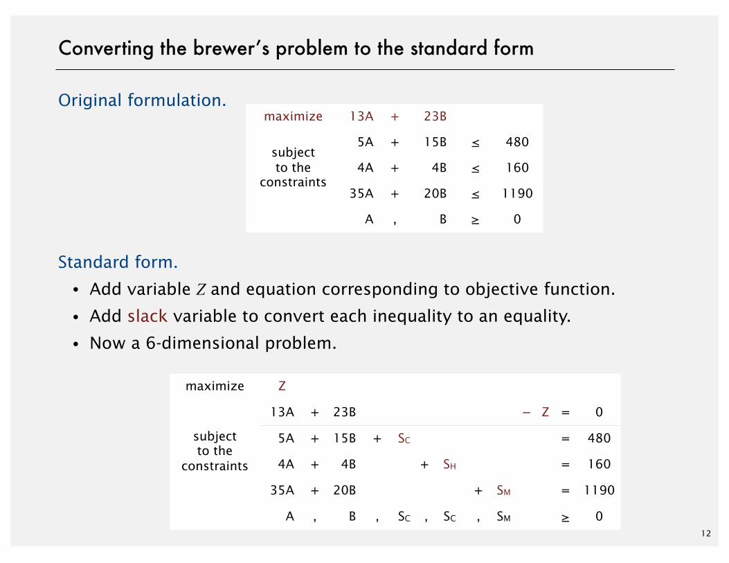
Converting the brewer’s problem to the standard form
Original formulation.
Standard form.
・Add variable Z and equation corresponding to objective function.
・Add slack variable to convert each inequality to an equality.
・Now a 6-dimensional problem.
maximize 13A + 23B
subjectto the
constraints
5A + 15B ≤ 480subjectto the
constraints 4A + 4B ≤ 160
subjectto the
constraints35A + 20B ≤ 1190
A , B ≥ 0
maximize Z
subjectto the
constraints
13A + 23B − Z = 0
subjectto the
constraints
5A + 15B + SCSC = 480subjectto the
constraints 4A + 4B + SHSHSH = 160
subjectto the
constraints
35A + 20B ++ SMSM = 1190
A , B , SCSC , SCSCSC ,, SMSM ≥ 0
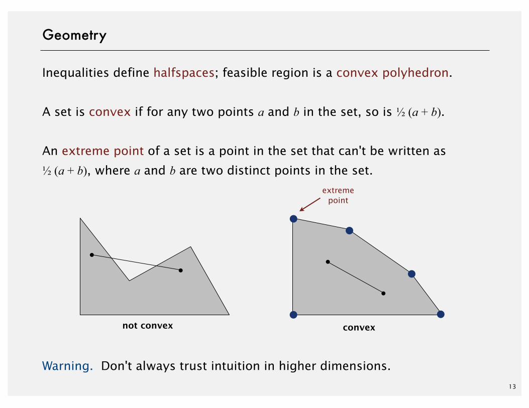
Inequalities define halfspaces; feasible region is a convex polyhedron.
A set is convex if for any two points a and b in the set, so is ½ (a + b).
An extreme point of a set is a point in the set that can't be written as
½ (a + b), where a and b are two distinct points in the set.
Warning. Don't always trust intuition in higher dimensions.13
Geometry
convexnot convex
extreme point
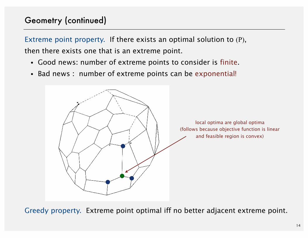
Extreme point property. If there exists an optimal solution to (P),then there exists one that is an extreme point.
・Good news: number of extreme points to consider is finite.
・Bad news : number of extreme points can be exponential!
Greedy property. Extreme point optimal iff no better adjacent extreme point.
14
Geometry (continued)
local optima are global optima(follows because objective function is linear
and feasible region is convex)
http://algs4.cs.princeton.edu
ROBERT SEDGEWICK | KEVIN WAYNE
Algorithms
‣ brewer’s problem
‣ simplex algorithm
‣ implementations
‣ reductions
LINEAR PROGRAMMING
http://algs4.cs.princeton.edu
ROBERT SEDGEWICK | KEVIN WAYNE
Algorithms
‣ brewer’s problem
‣ simplex algorithm
‣ implementations
‣ reductions
LINEAR PROGRAMMING
17
Simplex algorithm
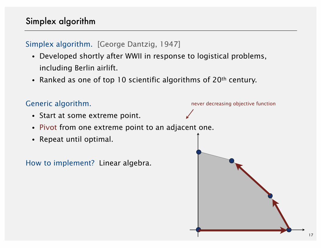
Simplex algorithm. [George Dantzig, 1947]
・Developed shortly after WWII in response to logistical problems,
including Berlin airlift.
・Ranked as one of top 10 scientific algorithms of 20th century.
Generic algorithm.
・Start at some extreme point.
・Pivot from one extreme point to an adjacent one.
・Repeat until optimal.
How to implement? Linear algebra.
never decreasing objective function
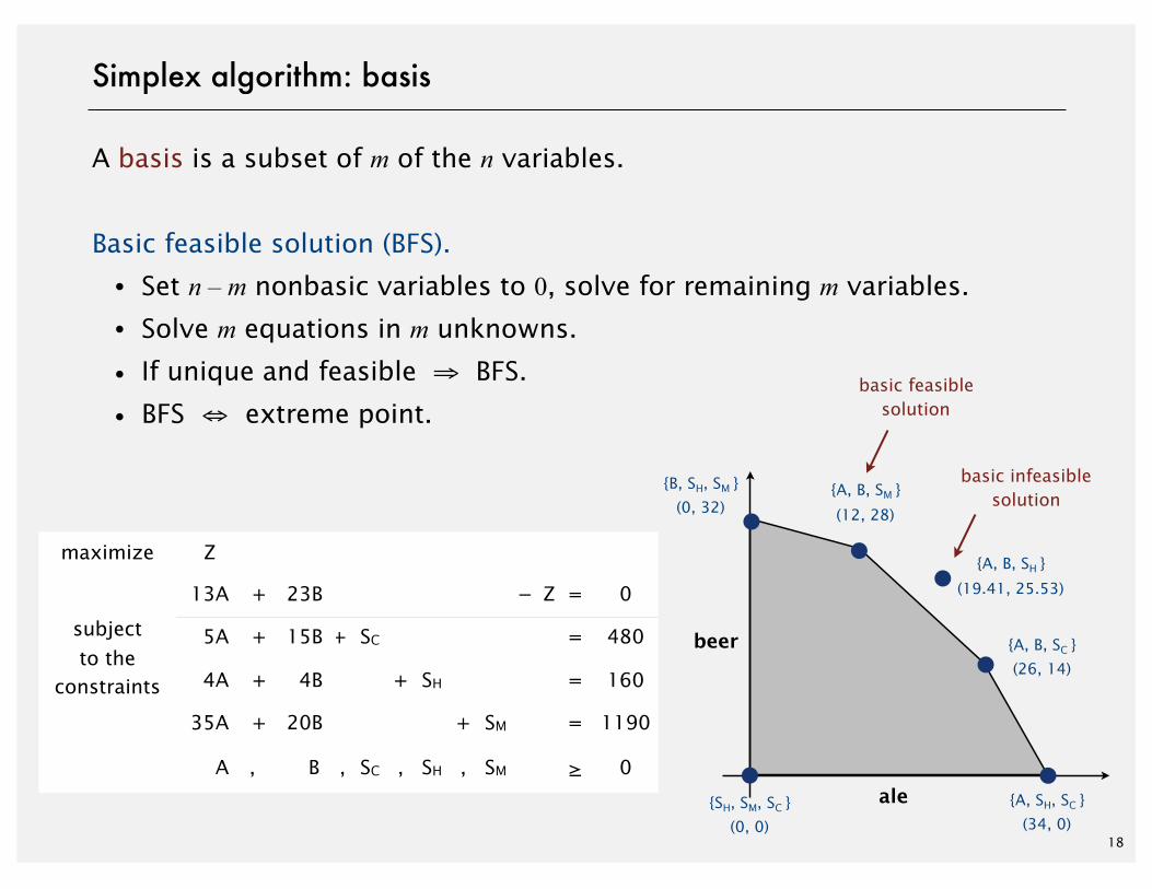
A basis is a subset of m of the n variables.
Basic feasible solution (BFS).
・Set n – m nonbasic variables to 0, solve for remaining m variables.
・Solve m equations in m unknowns.
・If unique and feasible ⇒ BFS.
・BFS ⇔ extreme point.
{B, SH, SM }
(0, 32)
{SH, SM, SC }
(0, 0)
{A, SH, SC }
(34, 0)
{A, B, SC }
(26, 14)
18
Simplex algorithm: basis
ale
beer
maximize Z
subjectto the
constraints
13A + 23B − Z = 0
subjectto the
constraints
5A + 15B + SC = 480subjectto the
constraints 4A + 4B + SH = 160
subjectto the
constraints
35A + 20B + SM = 1190
A , B , SC , SH , SM ≥ 0
{A, B, SM }
(12, 28)
basic feasiblesolution
{A, B, SH }
(19.41, 25.53)
basic infeasiblesolution
maximize Z
subjectto the
constraints
13A + 23B − Z = 0
subjectto the
constraints
5A + 15B + SC = 480subjectto the
constraints 4A + 4B + SH = 160
subjectto the
constraints
35A + 20B + SM = 1190
A , B , SC , SH , SM ≥ 0
19
Simplex algorithm: initialization
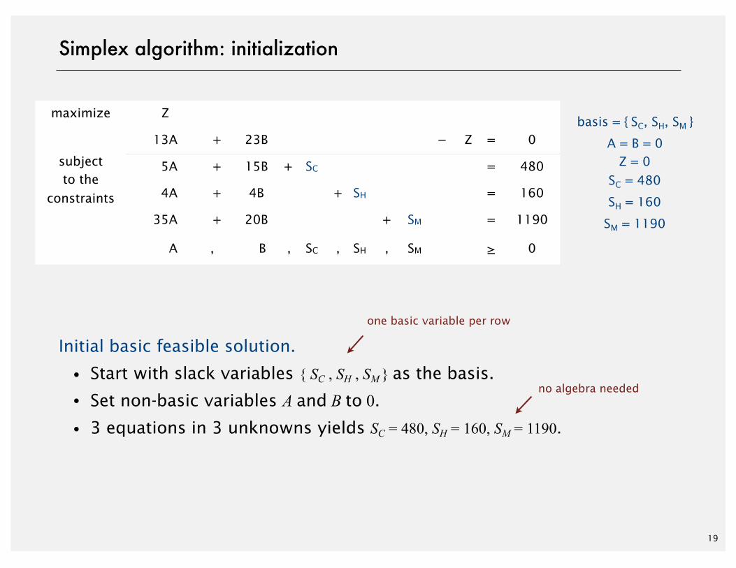
Initial basic feasible solution.
・Start with slack variables { SC , SH , SM } as the basis.
・Set non-basic variables A and B to 0.
・3 equations in 3 unknowns yields SC = 480, SH = 160, SM = 1190.
no algebra needed
basis = { SC, SH, SM }
A = B = 0Z = 0
SC = 480
SH = 160
SM = 1190
one basic variable per row
basis = { SC, SH, SM }
A = B = 0Z = 0
SC = 480
SH = 160
SM = 1190
20
Simplex algorithm: pivot 1
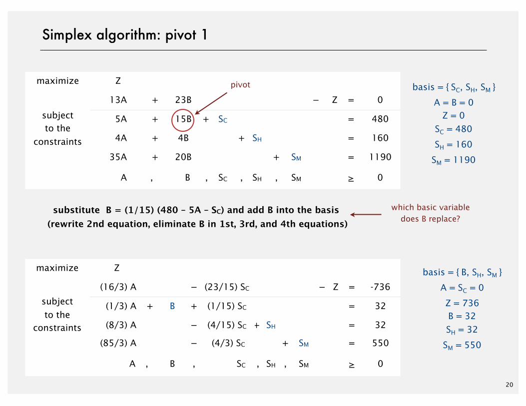
substitute B = (1/15) (480 – 5A – SC) and add B into the basis (rewrite 2nd equation, eliminate B in 1st, 3rd, and 4th equations)
basis = { B, SH, SM }
A = SC = 0
Z = 736B = 32 SH = 32
SM = 550
maximize Z
subjectto the
constraints
(16/3) A − (23/15) SC − Z = -736
subjectto the
constraints
(1/3) A + B + (1/15) SC = 32subjectto the
constraints (8/3) A − (4/15) SC + SH = 32
subjectto the
constraints
(85/3) A − (4/3) SC + SM = 550
A , B , SC , SH , SM ≥ 0
which basic variabledoes B replace?
maximize Z
subjectto the
constraints
13A + 23B − Z = 0
subjectto the
constraints
5A + 15B + SC = 480subjectto the
constraints 4A + 4B + SH = 160
subjectto the
constraints
35A + 20B + SM = 1190
A , B , SC , SH , SM ≥ 0
pivot
21
Simplex algorithm: pivot 1
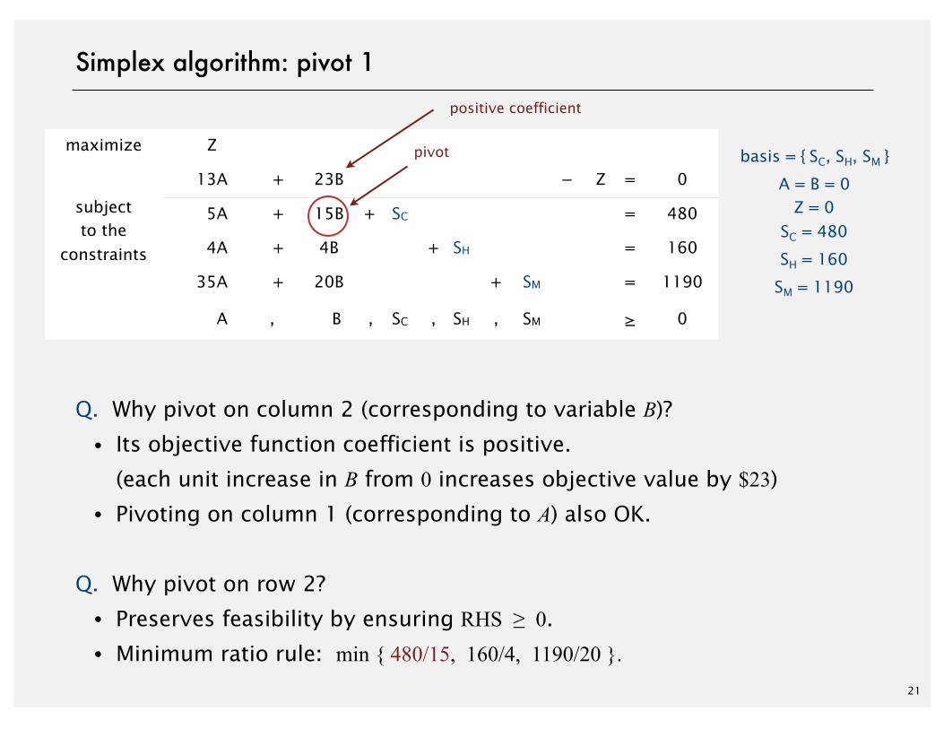
Q. Why pivot on column 2 (corresponding to variable B)?
・Its objective function coefficient is positive.
(each unit increase in B from 0 increases objective value by $23)
・Pivoting on column 1 (corresponding to A) also OK.
Q. Why pivot on row 2?
・Preserves feasibility by ensuring RHS ≥ 0.
・Minimum ratio rule: min { 480/15, 160/4, 1190/20 }.
basis = { SC, SH, SM }
A = B = 0Z = 0
SC = 480
SH = 160
SM = 1190
maximize Z
subjectto the
constraints
13A + 23B − Z = 0
subjectto the
constraints
5A + 15B + SC = 480subjectto the
constraints 4A + 4B + SH = 160
subjectto the
constraints
35A + 20B + SM = 1190
A , B , SC , SH , SM ≥ 0
pivot
positive coefficient
basis = { B, SH, SM }
A = SC = 0
Z = 736B = 32 SH = 32
SM = 550
maximize Z
subjectto the
constraints
(16/3) A − (23/15) SC − Z = -736
subjectto the
constraints
(1/3) A + B + (1/15) SC = 32subjectto the
constraints (8/3) A − (4/15) SC + SH = 32
subjectto the
constraints
(85/3) A − (4/3) SC + SM = 550
A , B , SC , SH , SM ≥ 0
22
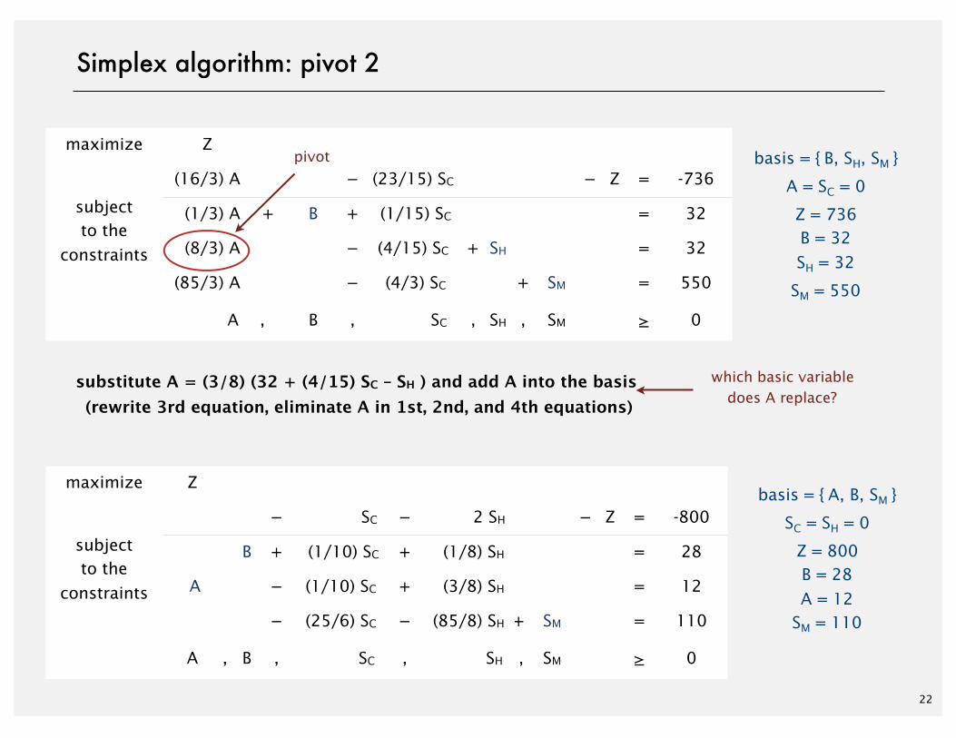
Simplex algorithm: pivot 2
basis = { A, B, SM }
SC = SH = 0
Z = 800B = 28 A = 12
SM = 110
maximize Z
subjectto the
constraints
− SC − 2 SH − Z = -800
subjectto the
constraints
B + (1/10) SC + (1/8) SH = 28subjectto the
constraints A − (1/10) SC + (3/8) SH = 12
subjectto the
constraints
− (25/6) SC − (85/8) SH + SM = 110
A , B , SC , SH , SM ≥ 0
pivot
substitute A = (3/8) (32 + (4/15) SC – SH ) and add A into the basis (rewrite 3rd equation, eliminate A in 1st, 2nd, and 4th equations)
which basic variabledoes A replace?
23
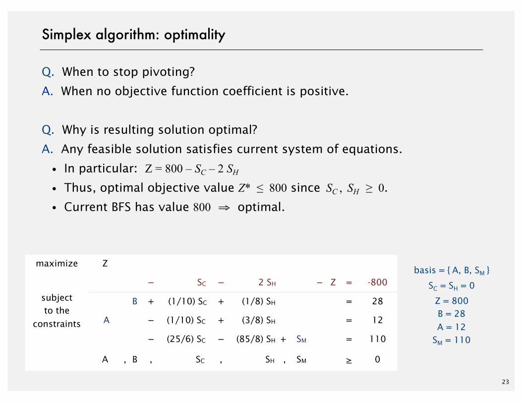
Simplex algorithm: optimality
Q. When to stop pivoting?
A. When no objective function coefficient is positive.
Q. Why is resulting solution optimal?
A. Any feasible solution satisfies current system of equations.
・In particular: Z = 800 – SC – 2 SH
・Thus, optimal objective value Z* ≤ 800 since SC , SH ≥ 0.
・Current BFS has value 800 ⇒ optimal.
basis = { A, B, SM }
SC = SH = 0
Z = 800B = 28 A = 12
SM = 110
maximize Z
subjectto the
constraints
− SC − 2 SH − Z = -800
subjectto the
constraints
B + (1/10) SC + (1/8) SH = 28subjectto the
constraints A − (1/10) SC + (3/8) SH = 12
subjectto the
constraints
− (25/6) SC − (85/8) SH + SM = 110
A , B , SC , SH , SM ≥ 0

http://algs4.cs.princeton.edu
ROBERT SEDGEWICK | KEVIN WAYNE
Algorithms
‣ brewer’s problem
‣ simplex algorithm
‣ implementations
‣ reductions
LINEAR PROGRAMMING

http://algs4.cs.princeton.edu
ROBERT SEDGEWICK | KEVIN WAYNE
Algorithms
‣ brewer’s problem
‣ simplex algorithm
‣ implementations
‣ reductions
LINEAR PROGRAMMING
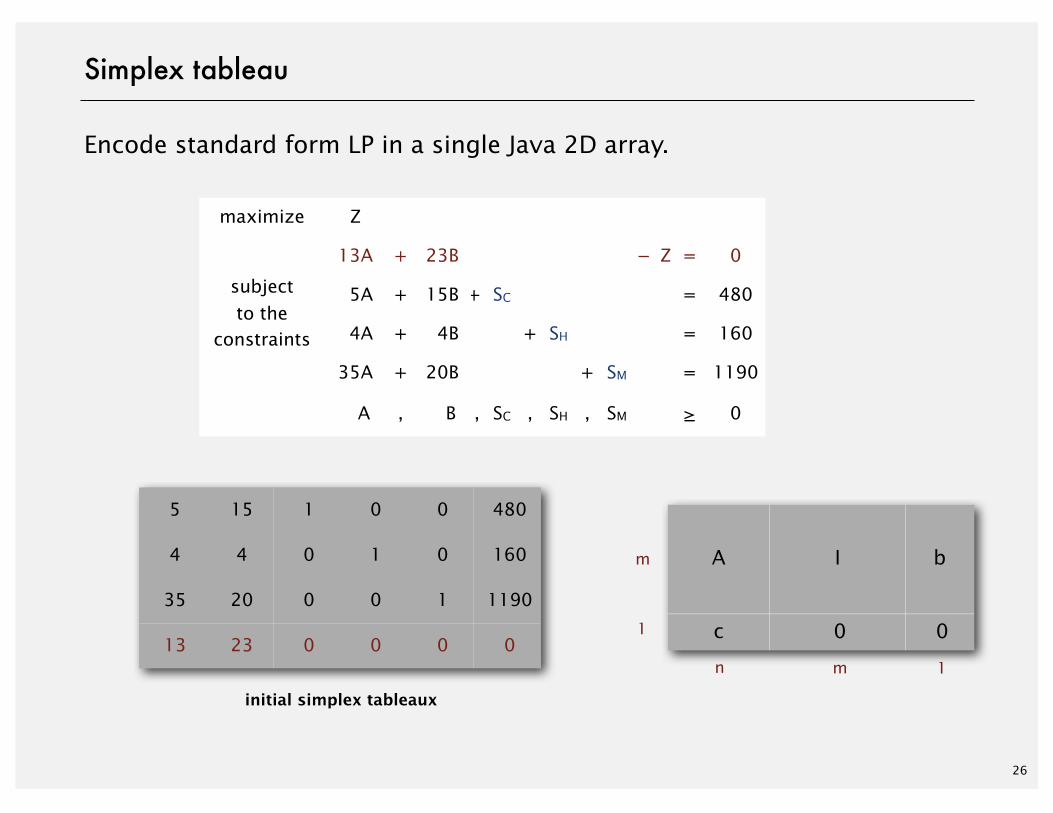
Encode standard form LP in a single Java 2D array.
Simplex tableau
26
m
1
n m 1
maximize Z
subjectto the
constraints
13A + 23B − Z = 0
subjectto the
constraints
5A + 15B + SC = 480subjectto the
constraints 4A + 4B + SH = 160
subjectto the
constraints
35A + 20B + SM = 1190
A , B , SC , SH , SM ≥ 0
initial simplex tableaux
5 15 1 0 0 480
4 4 0 1 0 160
35 20 0 0 1 1190
13 23 0 0 0 0
A I b
c 0 0
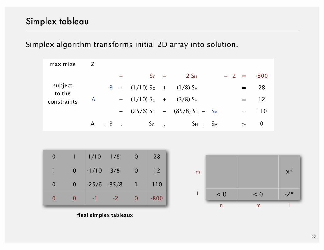
Simplex algorithm transforms initial 2D array into solution.
Simplex tableau
27
maximize Z
subjectto the
constraints
− SC − 2 SH − Z = -800
subjectto the
constraints
B + (1/10) SC + (1/8) SH = 28subjectto the
constraints A − (1/10) SC + (3/8) SH = 12
subjectto the
constraints
− (25/6) SC − (85/8) SH + SM = 110
A , B , SC , SH , SM ≥ 0
0 1 1/10 1/8 0 28
1 0 -1/10 3/8 0 12
0 0 -25/6 -85/8 1 110
0 0 -1 -2 0 -800
m
1
n m 1
x*
≤ 0 ≤ 0 -Z*
final simplex tableaux
28
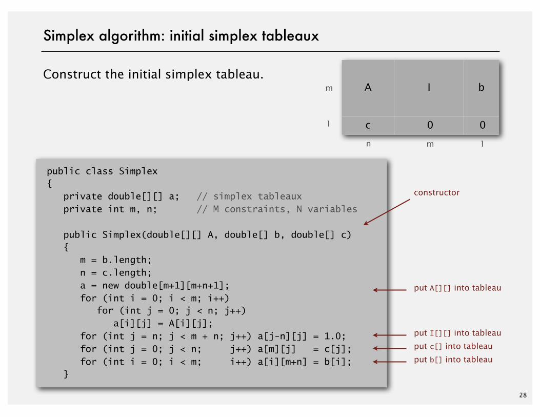
Simplex algorithm: initial simplex tableaux
Construct the initial simplex tableau.
public class Simplex{ private double[][] a; // simplex tableaux private int m, n; // M constraints, N variables
public Simplex(double[][] A, double[] b, double[] c) { m = b.length; n = c.length; a = new double[m+1][m+n+1]; for (int i = 0; i < m; i++) for (int j = 0; j < n; j++) a[i][j] = A[i][j]; for (int j = n; j < m + n; j++) a[j-n][j] = 1.0; for (int j = 0; j < n; j++) a[m][j] = c[j]; for (int i = 0; i < m; i++) a[i][m+n] = b[i]; }
put A[][] into tableau
put I[][] into tableau
put c[] into tableau
put b[] into tableau
constructor
m
1
n m 1
A I b
c 0 0
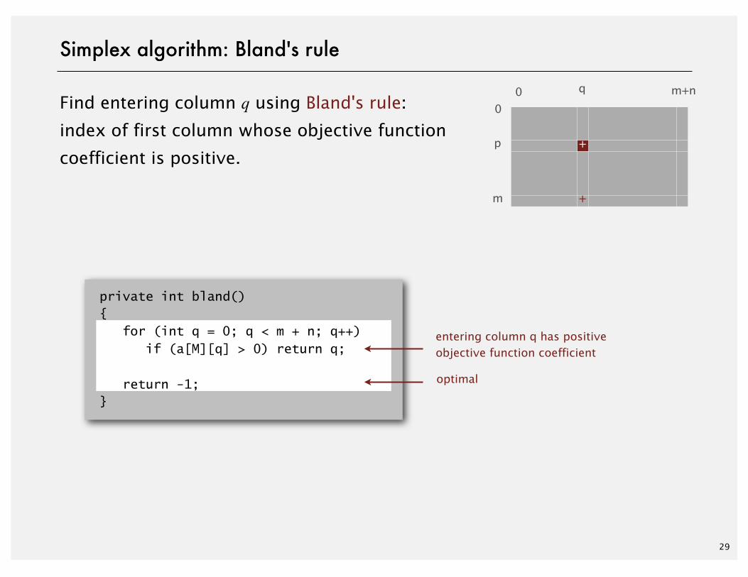
Find entering column q using Bland's rule:
index of first column whose objective function
coefficient is positive.
private int bland(){ for (int q = 0; q < m + n; q++) if (a[M][q] > 0) return q;
return -1;}
29
Simplex algorithm: Bland's rule
q
entering column q has positive objective function coefficient
optimal
m
m+n
00
+
+p
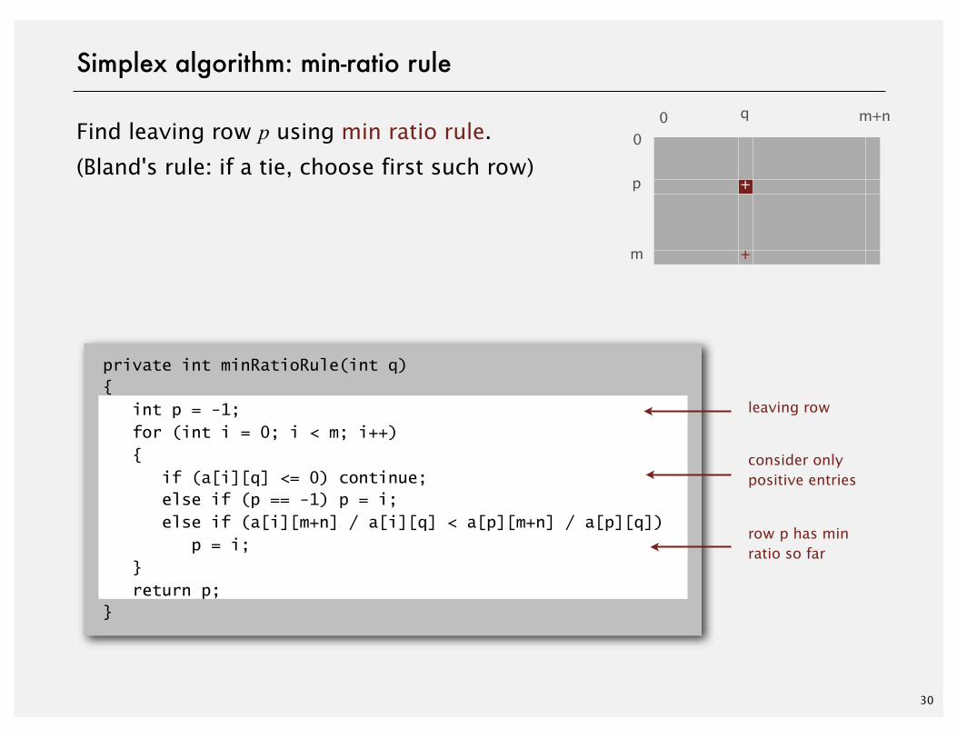
Find leaving row p using min ratio rule.
(Bland's rule: if a tie, choose first such row)
private int minRatioRule(int q){ int p = -1; for (int i = 0; i < m; i++) { if (a[i][q] <= 0) continue; else if (p == -1) p = i; else if (a[i][m+n] / a[i][q] < a[p][m+n] / a[p][q]) p = i; } return p;}
30
Simplex algorithm: min-ratio rule
leaving row
consider only positive entries
row p has min ratio so far
p
q
m
m+n
00
+
+
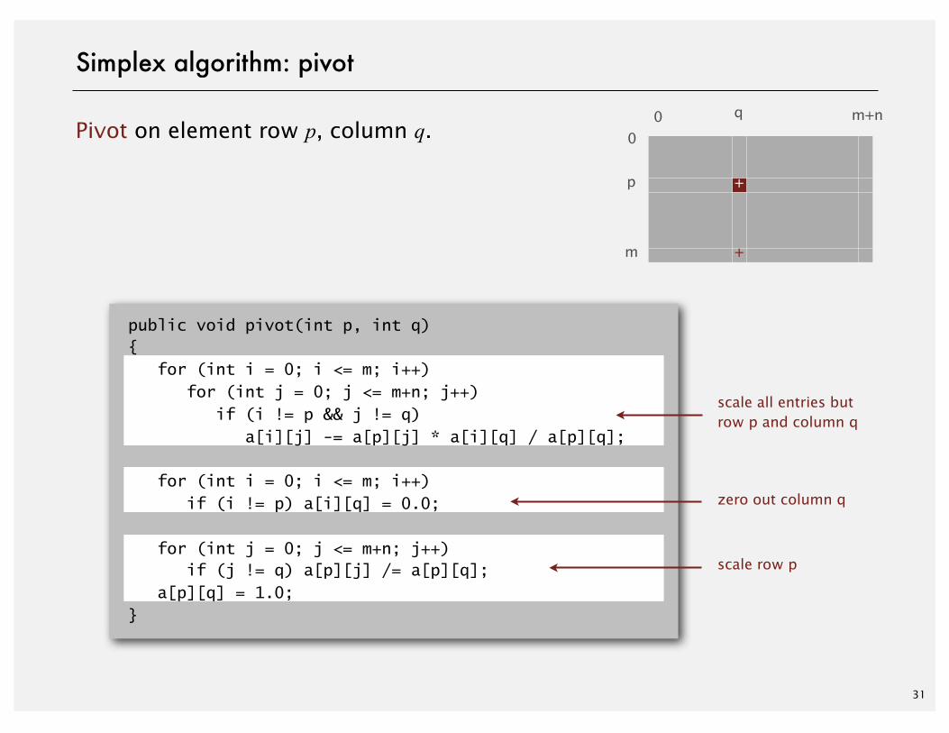
Pivot on element row p, column q.
public void pivot(int p, int q){ for (int i = 0; i <= m; i++) for (int j = 0; j <= m+n; j++) if (i != p && j != q) a[i][j] -= a[p][j] * a[i][q] / a[p][q]; for (int i = 0; i <= m; i++) if (i != p) a[i][q] = 0.0;
for (int j = 0; j <= m+n; j++) if (j != q) a[p][j] /= a[p][q]; a[p][q] = 1.0;}
31
Simplex algorithm: pivot
scale all entries butrow p and column q
zero out column q
scale row p
q
m
m+n
00
+
+p
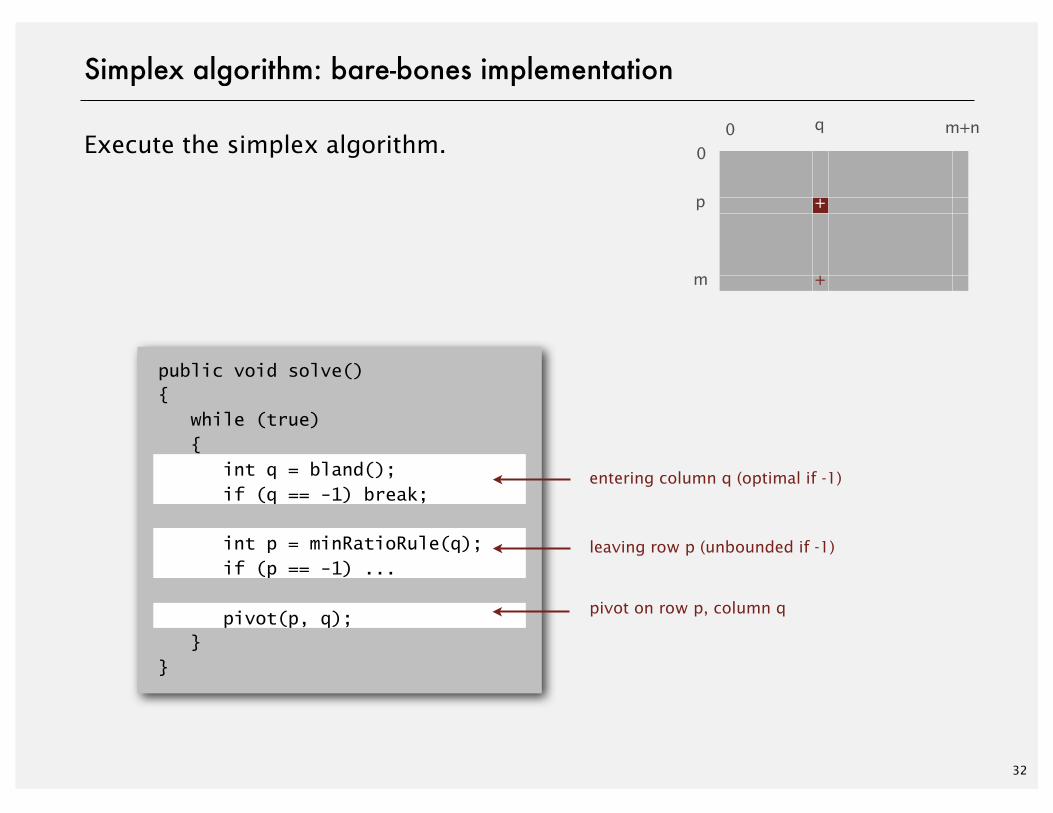
Execute the simplex algorithm.
public void solve(){ while (true) { int q = bland(); if (q == -1) break;
int p = minRatioRule(q); if (p == -1) ... pivot(p, q); }}
32
Simplex algorithm: bare-bones implementation
pivot on row p, column q
leaving row p (unbounded if -1)
entering column q (optimal if -1)
q
m
m+n
00
+
+p
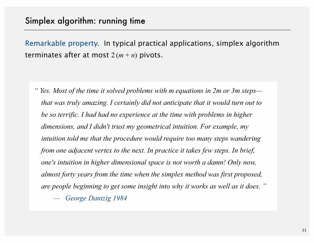
Remarkable property. In typical practical applications, simplex algorithm
terminates after at most 2 (m + n) pivots.
33
Simplex algorithm: running time
“ Yes. Most of the time it solved problems with m equations in 2m or 3m steps—
that was truly amazing. I certainly did not anticipate that it would turn out to
be so terrific. I had had no experience at the time with problems in higher
dimensions, and I didn't trust my geometrical intuition. For example, my
intuition told me that the procedure would require too many steps wandering
from one adjacent vertex to the next. In practice it takes few steps. In brief,
one's intuition in higher dimensional space is not worth a damn! Only now,
almost forty years from the time when the simplex method was first proposed,
are people beginning to get some insight into why it works as well as it does. ”
— George Dantzig 1984
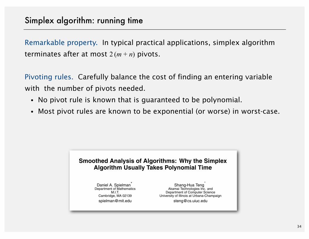
Remarkable property. In typical practical applications, simplex algorithm
terminates after at most 2 (m + n) pivots.
Pivoting rules. Carefully balance the cost of finding an entering variable
with the number of pivots needed.
・No pivot rule is known that is guaranteed to be polynomial.
・Most pivot rules are known to be exponential (or worse) in worst-case.
34
Simplex algorithm: running time
Smoothed Analysis of Algorithms: Why the SimplexAlgorithm Usually Takes Polynomial Time
Daniel A. SpielmanDepartment of Mathematics
M.I.T.Cambridge, MA 02139
Shang-Hua TengAkamai Technologies Inc. and
Department of Computer ScienceUniversity of Illinois at Urbana-Champaign
ABSTRACT
1. INTRODUCTION
Permission to make digital or hard copies of all or part of this work forpersonal or classroom use is granted without fee provided that copies arenot made or distributed for profit or commercial advantage and that copiesbear this notice and the full citation on the first page. To copy otherwise, torepublish, to post on servers or to redistribute to lists, requires prior specificpermission and/or a fee.STOC’01, July 6-8, 2001, Hersonissos, Crete, Greece.Copyright 2001 ACM 1-58113-349-9/01/0007 ... 5.00.
1.1 Background
296
35
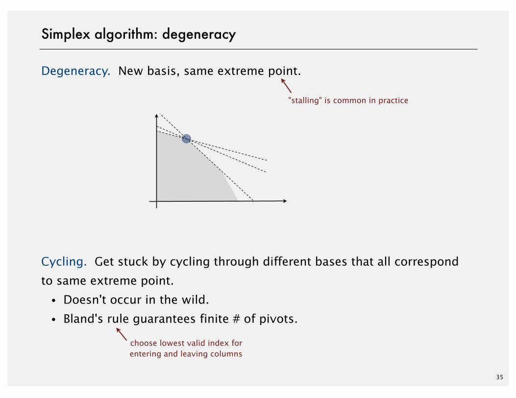
Simplex algorithm: degeneracy
Degeneracy. New basis, same extreme point.
Cycling. Get stuck by cycling through different bases that all correspond
to same extreme point.
・Doesn't occur in the wild.
・Bland's rule guarantees finite # of pivots.
"stalling" is common in practice
choose lowest valid index forentering and leaving columns
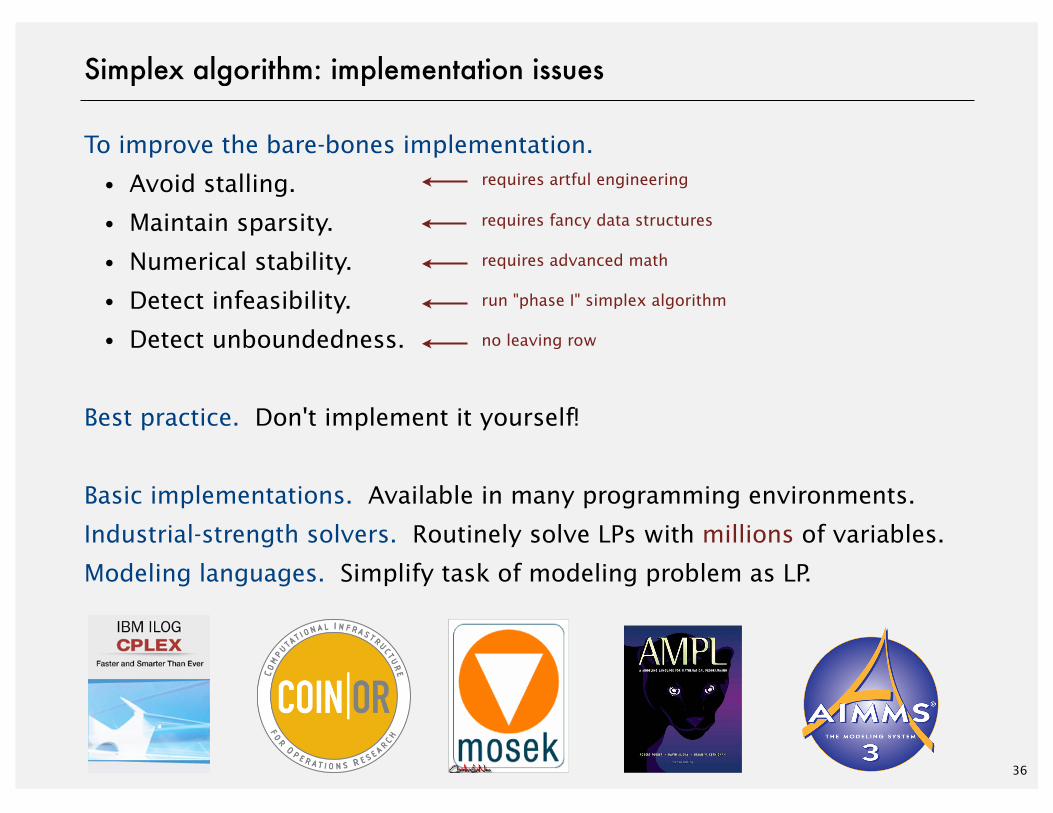
To improve the bare-bones implementation.
・Avoid stalling.
・Maintain sparsity.
・Numerical stability.
・Detect infeasibility.
・Detect unboundedness.
Best practice. Don't implement it yourself!
Basic implementations. Available in many programming environments.
Industrial-strength solvers. Routinely solve LPs with millions of variables.
Modeling languages. Simplify task of modeling problem as LP.
36
Simplex algorithm: implementation issues
requires fancy data structures
requires advanced math
run "phase I" simplex algorithm
no leaving row
requires artful engineering
37
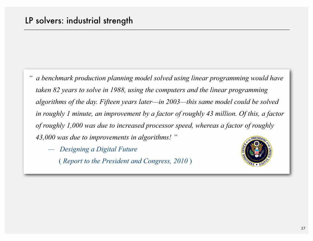
LP solvers: industrial strength
“ a benchmark production planning model solved using linear programming would have
taken 82 years to solve in 1988, using the computers and the linear programming
algorithms of the day. Fifteen years later—in 2003—this same model could be solved
in roughly 1 minute, an improvement by a factor of roughly 43 million. Of this, a factor
of roughly 1,000 was due to increased processor speed, whereas a factor of roughly
43,000 was due to improvements in algorithms! ”
— Designing a Digital Future
( Report to the President and Congress, 2010 )
38
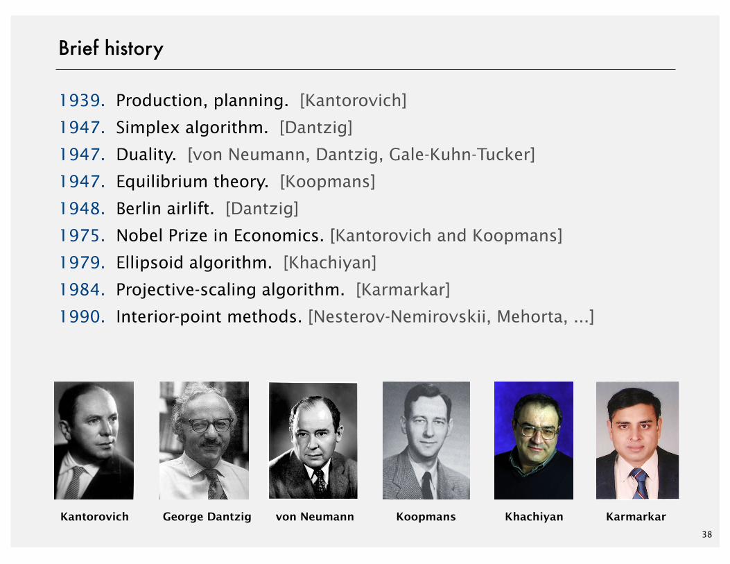
Brief history
1939. Production, planning. [Kantorovich]
1947. Simplex algorithm. [Dantzig]
1947. Duality. [von Neumann, Dantzig, Gale-Kuhn-Tucker]
1947. Equilibrium theory. [Koopmans]
1948. Berlin airlift. [Dantzig]
1975. Nobel Prize in Economics. [Kantorovich and Koopmans]
1979. Ellipsoid algorithm. [Khachiyan]
1984. Projective-scaling algorithm. [Karmarkar]
1990. Interior-point methods. [Nesterov-Nemirovskii, Mehorta, ...]
George Dantzig von Neumann Khachiyan KarmarkarKantorovich Koopmans
http://algs4.cs.princeton.edu
ROBERT SEDGEWICK | KEVIN WAYNE
Algorithms
‣ brewer’s problem
‣ simplex algorithm
‣ implementations
‣ reductions
LINEAR PROGRAMMING
http://algs4.cs.princeton.edu
ROBERT SEDGEWICK | KEVIN WAYNE
Algorithms
‣ brewer’s problem
‣ simplex algorithm
‣ implementations
‣ reductions
LINEAR PROGRAMMING
41
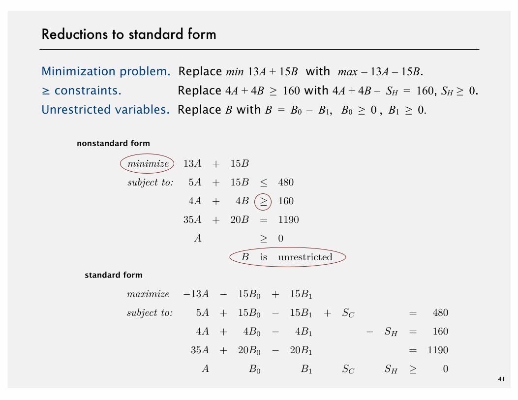
Reductions to standard form
Minimization problem. Replace min 13A + 15B with max – 13A – 15B.
≥ constraints. Replace 4A + 4B ≥ 160 with 4A + 4B – SH = 160, SH ≥ 0.
Unrestricted variables. Replace B with B = B0 – B1, B0 ≥ 0 , B1 ≥ 0.
13A + 15B
5A + 15B ≤ 480
4A + 4B ≥ 160
35A + 20B = 1190
A ≥ 0
B
−13A − 15B0 + 15B1
5A + 15B0 − 15B1 + SC = 480
4A + 4B0 − 4B1 − SH = 160
35A + 20B0 − 20B1 = 1190
A B0 B1 SC SH ≥ 0
nonstandard form
standard form
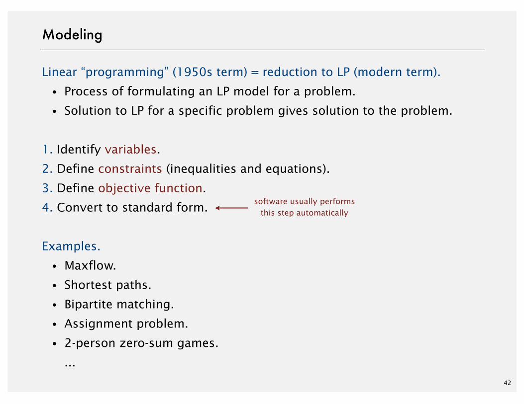
Linear “programming” (1950s term) = reduction to LP (modern term).
・Process of formulating an LP model for a problem.
・Solution to LP for a specific problem gives solution to the problem.
1. Identify variables.
2. Define constraints (inequalities and equations).
3. Define objective function.
4. Convert to standard form.
Examples.
・Maxflow.
・Shortest paths.
・Bipartite matching.
・Assignment problem.
・2-person zero-sum games.
...
Modeling
42
software usually performsthis step automatically
43
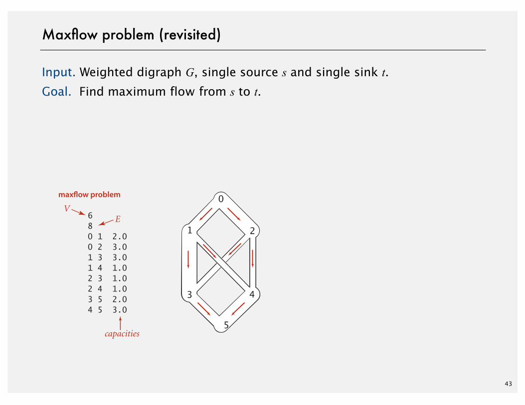
Maxflow problem (revisited)
Input. Weighted digraph G, single source s and single sink t.Goal. Find maximum flow from s to t.
Example of reducing network flow to linear programming
LP solution
maxflow problem maxflow solution
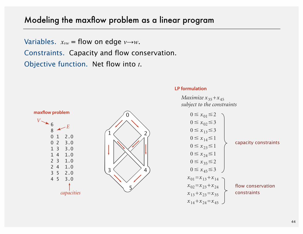
LP formulation
capacities
6 80 1 2.00 2 3.01 3 3.01 4 1.02 3 1.02 4 1.03 5 2.04 5 3.0
VE
0 ! x 01 ! 20 ! x 02 ! 30 ! x 13 ! 30 ! x 14 ! 10 ! x 23 ! 10 ! x 24 ! 10 ! x 35 ! 20 ! x 45 ! 3
x 01 = x 13 + x 14
x 02 = x 23 + x 24
x 13 + x 23 = x 35
x 14 + x 24 = x 45
Maximize x 35 + x 45subject to the constraints
x 01 = 2x 02 = 2x 13 = 1x 14 = 1x 23 = 1x 24 = 1x 35 = 2x 45 = 2
Max flow from 0 to 5
0->2 3.0 2.0
0->1 2.0 2.0
1->4 1.0 1.0
1->3 3.0 1.0
2->3 1.0 1.0
2->4 1.0 1.0
3->5 2.0 2.0
4->5 3.0 2.0
Max flow value: 4.0
Example of reducing network flow to linear programming
LP solution
maxflow problem maxflow solution
LP formulation
capacities
6 80 1 2.00 2 3.01 3 3.01 4 1.02 3 1.02 4 1.03 5 2.04 5 3.0
VE
0 ! x 01 ! 20 ! x 02 ! 30 ! x 13 ! 30 ! x 14 ! 10 ! x 23 ! 10 ! x 24 ! 10 ! x 35 ! 20 ! x 45 ! 3
x 01 = x 13 + x 14
x 02 = x 23 + x 24
x 13 + x 23 = x 35
x 14 + x 24 = x 45
Maximize x 35 + x 45subject to the constraints
x 01 = 2x 02 = 2x 13 = 1x 14 = 1x 23 = 1x 24 = 1x 35 = 2x 45 = 2
Max flow from 0 to 5
0->2 3.0 2.0
0->1 2.0 2.0
1->4 1.0 1.0
1->3 3.0 1.0
2->3 1.0 1.0
2->4 1.0 1.0
3->5 2.0 2.0
4->5 3.0 2.0
Max flow value: 4.0
44
Modeling the maxflow problem as a linear program
Variables. xvw = flow on edge v→w.
Constraints. Capacity and flow conservation.
Objective function. Net flow into t.
Example of reducing network flow to linear programming
LP solution
maxflow problem maxflow solution
LP formulation
capacities
6 80 1 2.00 2 3.01 3 3.01 4 1.02 3 1.02 4 1.03 5 2.04 5 3.0
VE
0 ! x 01 ! 20 ! x 02 ! 30 ! x 13 ! 30 ! x 14 ! 10 ! x 23 ! 10 ! x 24 ! 10 ! x 35 ! 20 ! x 45 ! 3
x 01 = x 13 + x 14
x 02 = x 23 + x 24
x 13 + x 23 = x 35
x 14 + x 24 = x 45
Maximize x 35 + x 45subject to the constraints
x 01 = 2x 02 = 2x 13 = 1x 14 = 1x 23 = 1x 24 = 1x 35 = 2x 45 = 2
Max flow from 0 to 5
0->2 3.0 2.0
0->1 2.0 2.0
1->4 1.0 1.0
1->3 3.0 1.0
2->3 1.0 1.0
2->4 1.0 1.0
3->5 2.0 2.0
4->5 3.0 2.0
Max flow value: 4.0
flow conservationconstraints
capacity constraints
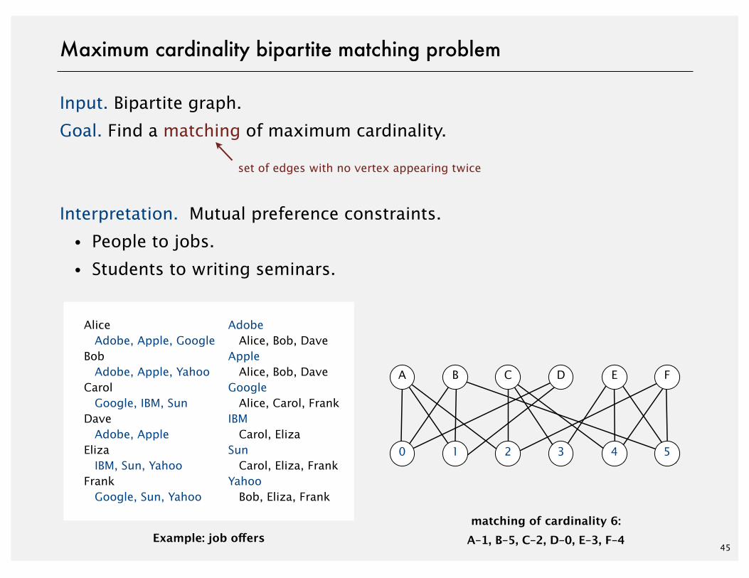
Input. Bipartite graph.
Goal. Find a matching of maximum cardinality.
Interpretation. Mutual preference constraints.
・People to jobs.
・Students to writing seminars.
Maximum cardinality bipartite matching problem
A B C D E F
0 1 2 3 4 5
Alice Adobe, Apple, GoogleBob Adobe, Apple, YahooCarol Google, IBM, SunDave Adobe, AppleEliza IBM, Sun, YahooFrank Google, Sun, Yahoo
Example: job offers
Adobe Alice, Bob, DaveApple Alice, Bob, DaveGoogle Alice, Carol, FrankIBM Carol, ElizaSun Carol, Eliza, FrankYahoo Bob, Eliza, Frank
45
matching of cardinality 6:A–1, B–5, C–2, D–0, E–3, F–4
set of edges with no vertex appearing twice
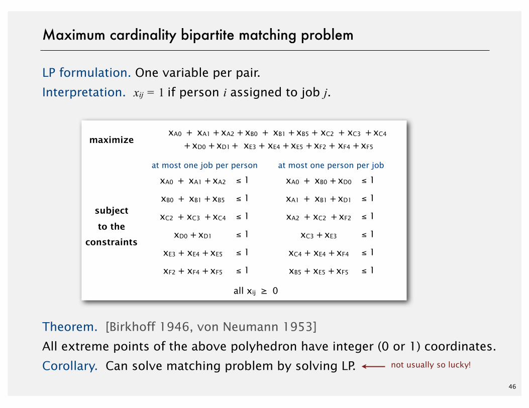
LP formulation. One variable per pair.
Interpretation. xij = 1 if person i assigned to job j.
Theorem. [Birkhoff 1946, von Neumann 1953]
All extreme points of the above polyhedron have integer (0 or 1) coordinates.
Corollary. Can solve matching problem by solving LP.46
Maximum cardinality bipartite matching problem
maximizexA0 + xA1 + xA2 +
+ xD0 + xD1 + xA2 + xB0
D1 + xE3 + xxB0 + xB1
E3 + xE4 +xB1 + xB5 + xC2 + xC3
E4 + xE5 + xF2 + xF4 + xC3 + xC4
+ xF5
xA0 + xA1 + xA2 ≤ 1 xA0 + xB0 + xD0 ≤ 1
subjectxB0 + xB1 + xB5 ≤ 1 xA1 + xB1 + xD1 ≤ 1
subjectto the
xC2 + xC3 + xC4 ≤ 1 xA2 + xC2 + xF2 ≤ 1to the
constraintsxD0 + xD1 ≤ 1 xC3 + xE3 ≤ 1
constraintsxE3 + xE4 + xE5 ≤ 1 xC4 + xE4 + xF4 ≤ 1
xF2 + xF4 + xF5 ≤ 1 xB5 + xE5 + xF5 ≤ 1
all xall xij ≥all xij ≥ 00
at most one job per person
not usually so lucky!
at most one person per job
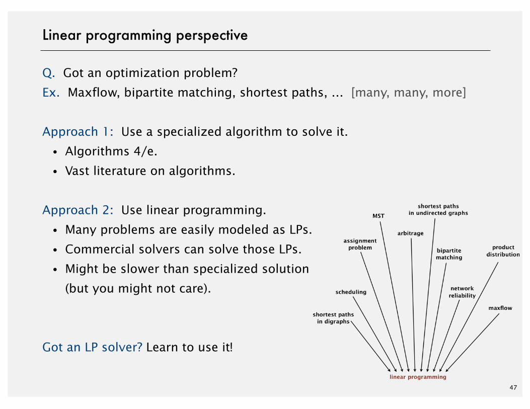
Q. Got an optimization problem?
Ex. Maxflow, bipartite matching, shortest paths, … [many, many, more]
Approach 1: Use a specialized algorithm to solve it.
・Algorithms 4/e.
・Vast literature on algorithms.
Approach 2: Use linear programming.
・Many problems are easily modeled as LPs.
・Commercial solvers can solve those LPs.
・Might be slower than specialized solution
(but you might not care).
Got an LP solver? Learn to use it!
Linear programming perspective
47
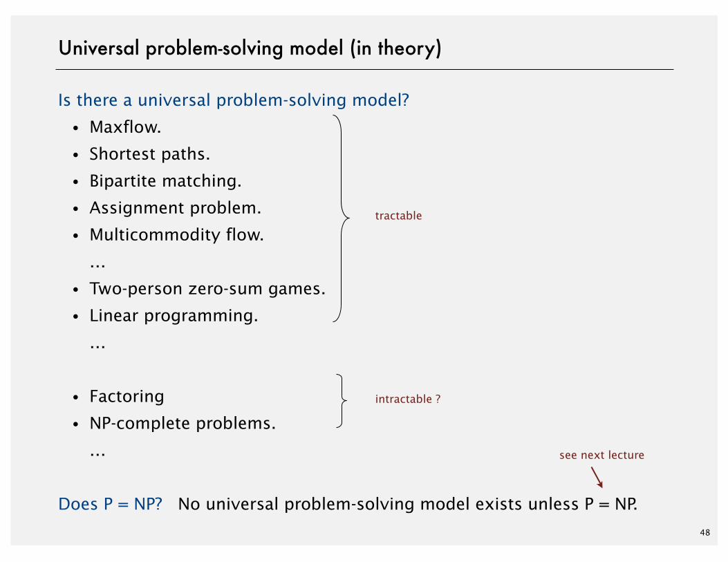
Is there a universal problem-solving model?
・Maxflow.
・Shortest paths.
・Bipartite matching.
・Assignment problem.
・Multicommodity flow.
…
・Two-person zero-sum games.
・Linear programming.
…
・Factoring
・NP-complete problems.
…
Does P = NP? No universal problem-solving model exists unless P = NP.48
Universal problem-solving model (in theory)
tractable
see next lecture
intractable ?

http://algs4.cs.princeton.edu
ROBERT SEDGEWICK | KEVIN WAYNE
Algorithms
‣ brewer’s problem
‣ simplex algorithm
‣ implementations
‣ reductions
LINEAR PROGRAMMING
ROBERT SEDGEWICK | KEVIN WAYNE
F O U R T H E D I T I O N
Algorithms
http://algs4.cs.princeton.edu
Algorithms ROBERT SEDGEWICK | KEVIN WAYNE
LINEAR PROGRAMMING
‣ brewer’s problem
‣ simplex algorithm
‣ implementations
‣ reductions
![Development of NeuroMat Open Databases [Computational Issues] · Fabio Kon (IME – USP) Kelly R. Braghetto (IME – USP) Collaborators (up to now)](https://img.pdfslide.us/doc/110x75/5c04d33b09d3f28b388c5baf/development-of-neuromat-open-databases-computational-issues-fabio-kon-ime.jpg)