Reaenhaa IME-USP 1993, Vol. 1, No.1, 46 - 56.

The Operational-Bayesian Approach In Reliability Theory

Richard E. Barlow1 and Max B. Mendel2

Abstract: We emphasize the derivation of likelihood models starting from a well specified problem of interest and finite populations. "Parameters" are given operational mean­ing. In particular, parameters are specified in terms of differ­ent forms of energy. Examples relevant to reliability theory are used to illustrate ideas. Examples in engineering probability are given.

Key words: Exchangeability, isotropicity, indifference, predictive probability, symmetry.

1. Introduction.

The key ingredients in this approach are an emphasis on 1) the operational meaning of questions posed and 2) the related field of specialization within which questions are posed . Deterministic and logical relationships basic to the field of application are used in part to develop appropriate probability models.

This approach requires a deeper understanding of the questions posed than the traditional approach and is consequently less mechanical in its application. P. A. W. Bridgman (1927) was perhaps first to popularize use of the term "op­erational" in the context of physical phenomena. De Finetti was one of the first to consider this approach in the context of probability theory. Dawid (1982) fol­lowed de Finetti's point of view by deriving subjective probability models based on observable random quantities. Mendel (1989) used the same approach but more closely followed Savage (1954) in placing emphasis on the decision prob­lem. Mendel advocates the "indifference principle" among acts as a means for constructing likelihood probability models.

We begin an operational-Bayesian analysis with a question or questions which require selection of an act or a decision. Like Lindley (1985 p . 4) we make no distinction between action and decision. The question or decision problem must contain terms which have operational meaning. That is, a bet based on the outcome related to our decision must have the property that it can be settled, at least in principle. We think about a value function relative to our problem . Value functions suggest "parameters" of interest. Although in practice it may be difficult to specify a value function, thinking about one helps identify "parameters"; i.e., functions of relevant but unknown observables. In general, value functions will

1 Research partially supported by the u.s. Air Force Office of Scientific Research (F49620-

93-1-001) grant and by the Army Research Office (DAAL03-91-G-0046) grant to the University

of California at Berkeley.

2 Research partially supported by the Army Research Office (DAAL03-91-G-0046) grant to

the University of California at Berkeley.

46

The Operational-Bayesian Approach In Reliability Theory 47

depend on these parameters. Parameters may be additive functions of observables. Examples of relevant "parameters" are energy, mass, force, money, etc. The value function and associated parameters together will determine the relevant sample space.

2. The Indifference Principle.

We propose that probability is essentially an analytical tool based on judg­ment. As an analytical tool, it plays a key role in decision making and forecasting. Its assessment, based on judgment, is the most difficult aspect. In the absence of a well defined, real problem, we can at most determine a conditional probability; e.g., a likelihood function. Even this probability function can only apply to a particular class of problems.

To illustrate the role of indifference in probability modeling, we will consider several cases where the parameter of interest is energy. Although energy can take many forms, it is conserved and it is additive.

2.1. Kinetic Energy of a Particle in Motion.

Consider a particle in an ideal gas in stable equilibrium. The gas particle is moving in space with a velocity whose coordinates in three mutually orthogonal directions can be represented by a velocity vector

The condition of stable equilibrium implies that the probability distribution of the velocity does not depend on the choice of the coordinates and hence that this random velocity vector is rotationally symmetric. Since kinetic energy is proportional to the sum of squares of the coordinate velocities when the mass is known, the parameter of interest corresponds,in this case, to the square of the f2-norm, namely

3

LX; = 302 .

;=1

Hence we would be indifferent between any two velocity vectors having the same sum of squares. This means that we would give the same predictive prob­ability (or probability density) for any two such vectors. It can be shown that the bivariate density for two coordinate velocities, conditional on the kinetic en­ergy, is determined by this indifference. The conditional bivariate density for two coordinate velocities can be shown to be

(1)

48 Richard E . Barlow and Max B. Mendel

for :i:~ + :i:~ 5 302 and 0 elsewhere.

2.2. eq-isotropic distributions.

If the joint distribution of XN is absolutely continuous, the parameter of interest may correspond to the eq-norm of XN . Considering the general case, suppose that our predictive probability function for XN has the property that p(XN) = p(YN) when XN and YN have the same eq-norm. We are in effect indifferent regarding vector outcomes having the same eq-norm. Even though our value function may depend on XN only through the eq-norm, it does not follow that we would always be indifferent to vector outcomes having the same eq-norm. As Lindley has pointed out, "My opinion about the data, were I to know the parameter, exists irrespective of the decision that might hinge on the data. To deny this would to fly in the face of scientific thinking which holds that pure science is meaningful."

In Barlow and Mendel (1992) we considered aging as well as the el-norm in deriving the likelihood.

The distribution of XN given E~l IXilq = NOq is singular, although p(xn I 0) exists for 1 5 n < N. In Mendel (1989), p(xn 10) is derived.

We have

for E~=l Ix;jq 5 NOq and 0 elsewhere.

For N - 00 and q = 2 we obtain the product of n independent normal densities where the parameter is the variance.

3. Strength of Materials.

The theory of static stress was, in many respects, developed in the last cen­tury. A very good reference to this subject is the book by Hoffman and Sachs (1953). However, the operational approach to the assessment of probability forms on the space of stress tensors is a very new subject still under development. More advanced results than those described below will appear in a forthcoming mono­graph by Mendel and Chick (1994).

3.1. Tensile Tests for Isotropic Ductile Materials.

Lindquist (1992) makes use of the el-norm model relative to the strength of ductile materials. When the distortion energy Ul of a material reaches a threshold

The Operational-Bayesian Approach In Reliability Theory 49

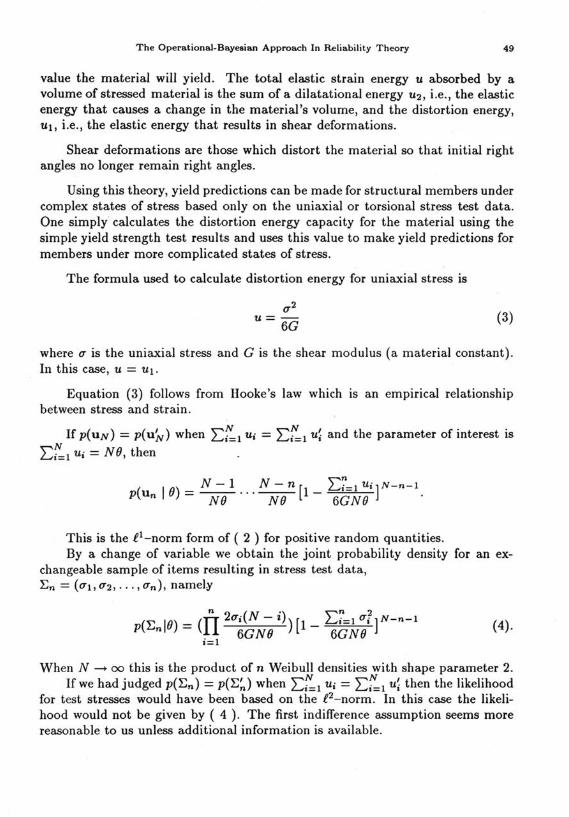
value the material will yield. The total elastic strain energy U absorbed by a volume of stressed material is the sum of a dilatational energy U2, i.e., the elastic energy that causes a change in the material's volume, and the distortion energy, Ul, i.e., the elastic energy that results in shear deformations.

Shear deformations are those which distort the material so that initial right angles no longer remain right angles.

Using this theory, yield predictions can be made for structural members under complex states of stress based only on the uniaxial or torsional stress test data. One simply calculates the distortion energy capacity for the material using the simple yield strength test results and uses this value to make yield predictions for members under more complicated states of stress.

The formula used to calculate distortion energy for uniaxial stress is

(3)

where U is the uniaxial stress and G is the shear modulus (a material constant) . In this case, U = Ul.

Equation (3) follows from Hooke's law which is an empirical relationship between stress and strain.

If P(UN) = P(uN) when 2:::1 Uj = 2:::1 ui and the parameter of interest is

2:::1 Uj = NO, then

( 1 0) = N -1 ... N - n [1- 2:7-1 U i 1N-n-l P Un NO NO 6GNO .

This is the fl-norm form of ( 2 ) for positive random quantities. By a change of variable we obtain the joint probability density for an ex­

changeable sample of items resulting in stress test data, En = (Ul, U2,···, Un), namely

(E 10) = (rrn 2Ui(N - i») [1- 2:7-1 ul(-n-l P n . 6GNO 6GNO

.=1 (4).

When N - 00 this is the product of n Weibull densities with shape parameter 2. If we had judged p(En) = p(E~) when 2:::1 Uj = 2:::1 u~ then the likelihood

for test stresSes would have been based on the f2-norm. In this case the likeli­hood would not be given by ( 4 ). The first indifference assumption seems more reasonable to us unless additional information is available.

50 Richard E . Barlow and Max B . Mendel

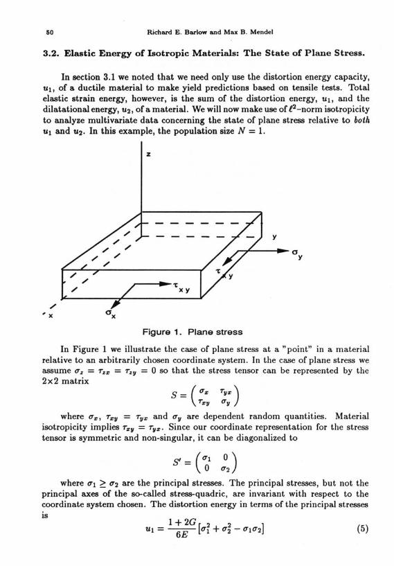
3.2. Elastic Energy of Isotropic Materials: The State of Plane Stress.

In section 3.1 we noted that we need only use the distortion energy capacity, U1, of a ductile material to make yield predictions based on tensile tests. Total elastic strain energy, however, is the sum of the distortion energy, U1, and the dilatational energy, U2, of a material. We will now make use of l2-norm isotropicity to analyze multivariate data concerning the state of plane stress relative to both U1 and U2. In this example, the population size N = 1.

" , x

" "

z

r---I~'t xy

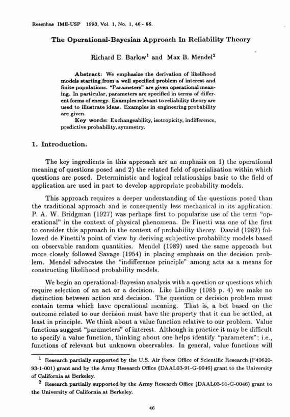
Figure 1. Plane stress

In Figure 1 we illustrate the case of plane stress at a "point" in a material relative to an arbitrarily chosen coordinate system. In the case of plane stress we asSume (1"z = r z ", = Tzy = 0 so that the stress tensor can be represented by the 2x2 matrix

S = ((1"", r y",) r",y (1"y

where (1""" T",y = Ty ", and (1"y are dependent random quantities. Material isotropicity implies T",y = Ty ",' Since our coordinate representation for the stress tensor is symmetric and non-singular, it can be diagonalized to

S'= (~1 ~J where (1"1 2: (1"2 are the principal stresses. The principal stresses, but not the

principal axes of the so-called stress-quadric, are invariant with respect to the coordinate system chosen. The distortion energy in terms of the principal stresses is

(5)

The Operational-Bayesian Approach In Reliabili t y Theory

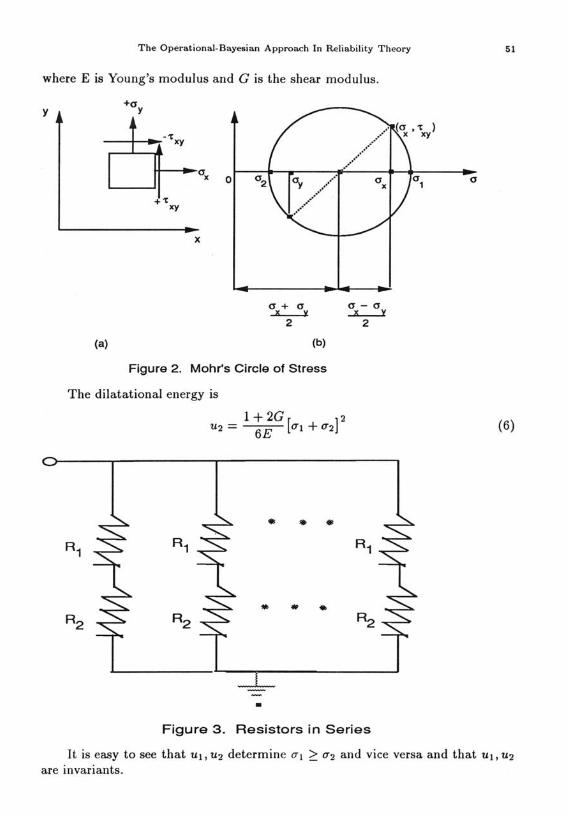
where E is Young's modulus and G is the shear modulus.

y

(a)

+'t xy

x

o

(b)

Figure 2. Mohr's Circle of Stress

The dilatational energy is

.. .. ..

..

•

•.. (0 • 't ) ••• x xy

......... ........

Figure 3. Resistors in Series

51

o

(6)

It is easy to see that U1, U2 determine 0"1 :::: 0"2 and vice versa and that U1, U2

are invariants.

52 Richard E. Barlow and Max B. Mendel

Conditional on U1 and U2 (or 1T1 and 1T2) we draw the so-called "Mohr circle" passing through (1T1' 0) and (1T2' 0) with center

Mohr's circle of stress (see Figure 2b) is widely used in practice for stress trans­formations.

Provided the initial stresses are given, the Mohr circle method is applicable whether the material behaves elastically or plastically.

Figure 2a shows the states of stress on a plane (in 3 dimensions) that would be determined by the x-axis. 1Tz: is the stress normal to this plane while rz:y is the stress parallel to this plane (the shearing stress). The dilatational energy, U2,

determines the center of the circle, namely

U1 and U2 together determine 1T1 ~ 1T2 which in turn determines the radius of the circle, namely

The radius of the circle corresponds to the maximum possible shear stress at the given point for planes orthogonal to the x-y plane. The point on the circle (IT z:, rz:y) corresponds to the state of stress on the plane determined by the x-axis which intersects the right hand face of the square in Figure 2a. In general, points on the circle correspond to the normal stress and the shearing stress on planes orthogonal to the x-y plane. We are indifferent to normal and shearing stresses corresponding to points on the circle by the laws governing the equilibrium of forces.

Since 2 _ 2 ( )2

r - rz:y + 1Tz: - ITm

p( IT z: 11T1' 1T2) can be calculated using (2-norm isotropicity to give

( I ) _~[1_(ITz:-lTm)21-1/2 P 1Tz: 1T1, 1T2 -1rr r

(7)

4. Lifetime Models.

The previous probability models were for multivariate observations on a single particle or a state of stress at a specified point in a body of isotropic material. The following example pertains to exchangeable observations on similar systems or units.

The Operational-Bayesian Approach In Reliability Theory 53

4.1. Lifetimes of Resistors in Series.

This section proposes an energy approach using an "energy potential" , rather than the classical failure rate, to specify classes of lifetime models. First, we con­sider the univariate case and the operating energy usage of N exchangeable resis­tors on the same voltage source. Such resistors could represent heating elements, light bulbs on a voltage source, turbines on a water reservoir of constant height; etc.

Let ai be the i-th unit's effective age which may be measured in units other than calendar time; e. g. cycles per second, etc. We call ai the aging rate for the i-th unit. This could, for example, be a derivative with respect to calendar time.

The energy usage of a single resistor with resistance Ri ohms is V 2 / Rs watts and its energy usage potential function becomes:

watts (or joules per second) if this is constant in the unit's age, ai. We call ai the aging rate for the i-th unit. This could, for example, depend on a specified maintenance policy. In any event it is specified although the unit's lifetime, Xi, is unknown. The energy potential evaluated at a unit's lifetime, Xi is

The lifetime energy usage for unit i is

If a unit's energy potential does not depend on the life of other units, then

N

LAi i=l

is the total lifetime energy used by a population of N units. If the parameter of interest is the average, namely

and we are indifferent to vectors of N lifetime energies having the same sum, then for

1 ~ n < N and by (1 isotropicity, we have

(8)

54 Richard E . Barlow and Max B . Mendel

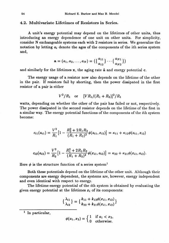
4.2. Multivariate Lifetimes of Resistors in Series.

A unit's energy potential may depend on the lifetimes of other units, thus introducing an energy dependence of one unit on other units. For simplicity, consider N exchangeable systems each with 2 resistors in series. We generalize the notation by letting ai denote the ages of the components of the ith series system and,

a = (aI, a2, ... ,aN) = ({ all } ... { aNI }) al2 aN2

and similarly for the lifetimes x, the aging rate Ii and energy potential c.

The energy usage of a resistor now also depends on the lifetime of the other in the pair. If resistors fail by shorting, then the power dissipated in the first resistor of a pair is either

watts, depending on whether the other of the pair has failed or not, respectively. The power dissipated in the second resistor depends on the lifetime of the first in a similar way. The energy potential functions of the components of the ith system become:

Here q, is the structure function of a series system I

Both these potentials depend on the lifetime of the other unit. Although their components are energy dependent, the systems are, however, energy independent and even identical with respect to energy.

The lifetime energy potential of the ith system is obtained by evaluating the given energy potential at the lifetimes Xi of its components:

I In particular,

The Operational-Bayesian Approach In Reliability Theory 55

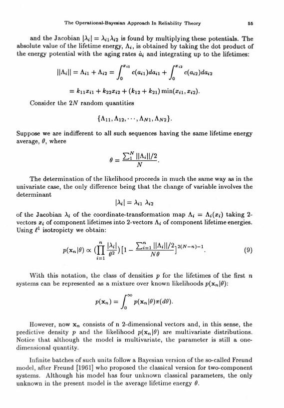
and the Jacobian IAi I = AilAi2 is found by multiplying these potentials. The absolute value of the lifetime energy, Ai, is obtained by taking the dot product of the energy potential with the aging rates ai and integrating up to the lifetimes:

= kllXil + k 22 X i2 + (k12 + k21 ) min(xil' Xi2).

Consider the 2N random quantities

Suppose we are indifferent to all such sequences having the same lifetime energy average, 0, where

0= 2:f IIAili/2 . N

The determination of the likelihood proceeds in much the same way as in the univariate case, the only difference being that the change of variable involves the determinant

IAi I = Ail Ai2

of the Jacobian Ai of the coordinate-transformation map Ai = Ai(Xi) taking 2-vectors Xi of component lifetimes into 2-vectors Ai of component lifetime energies. Using i 1 isotropicty we obtain:

p(xnIO) ex: (Jll:~') [1- 2:?=I;I:ill/2]2(N-n)-1.

i=1 (9)

With this notation, the class of densities P for the lifetimes of the first n systems can be represented as a mixture over known likelihoods p(xnIO):

However, now Xn consists of n 2-dimensional vectors and, in this sense, the predictive density P and the likelihood p(xn 10) are multivariate distributions. Notice that although the model is multivariate, the parameter is still a one­dimensional quantity.

Infinite batches of such units follow a Bayesian version of the so-called Freund model, after Freund [1961] who proposed the classical version for two-component systems. Although his model has four unknown classical parameters, the only unknown in the present model is the average lifetime energy O.

56 Richard E. Barlow and Max B . Mendel

5. Conclusions.

The likelihood model used to analyze data is surely as subjective as any "prior" probabilities. However, to make this model assessment we need to first concentrate on the question of interest and its relevant field of application. From the operational viewpoint statistical inference should be more closely associated with particular fields of application. This must occur if statistics is to be more than a cosmetic veneer attached to scientific papers.

6. References.

1 Barlow, R. E. and M. B. Mendel, "De Finetti-Type Representations for Life Distributions," Journal of the American Statistical Association, Vol. 87, Number 420, pp. 1116-1122, (1992).

2 Bridgman, P., The Logic of Modern Physics, New York, The Macmillan Co, (1927).

3 Dawid, A. P., "Intersubjective Statistical Models." Exchangeability in Prob­ability and Statistics, G . Koch and F. Spizzichino (edi tors), North-Holland Publishing Co, (1982).

4 De Finetti, B., "Foresight: Its Logical Laws, Its Subjective Sources." An­nales de l'Institute Henri Poincare 7, 1-68. English translation in Studies in Subjective Probability. Kyburg, H.E. Jr. , and Smokier, H.E., eds., 1980, (2nd ed.), Huntington, New York: Robert E. Krieger Pub . Co., pp. 53-118, (1937).

5 Freund, J . E., "A Bivariate Extension of the Exponential Distribution ." JASA 56: 971-977. Hoffman, O. and G. Sachs (1953) . Introduction to the Th eory of Plasticity for Engineers, New York, McGraw-Hill, ( 1961).

6 Lindley, D. V., Making Decisions, J . Wiley & Sons, New York , 2nd edi­tion,(1985).

7 Lindquist, E., "Strength of Materials and the Weibull Distribution ." UC Berkeley Technical Report ESRC 92-32 , Engineering Systems Research Cen­ter. To appear in the journal Probabilistic Engineering Mechanics, (1992).

8 Mendel, M. B. and S. Chick, The Geometry and Calculus of Engineering Prob­ability, Springer-Verlag. Mendel, M. B. (1991) . "An Economic Approach to Lifetime Modelling." UC Berkeley Technical Report ESRC 91-6 , Engineering Systems Research Center, (1994)

9 Mendel, M. B., Development of Bayesian Parametric Theory with Applica­tions to Control, MIT Ph.D. thesis, (1989).

10 Mendel, M. B., "Bayesian Parametric Models for Lifetimes." Bayesian Statis­tics 4. J . M. Bernardo, J . O . Berger, A. P. Dawid, and A. F. M. Smith, eds., Claredon Press, Oxford, 697-705, (1992).

11 Savage, 1. J., The Foundations of Statistics, New York: J. Wiley & Sons, (1954).