Embed Size (px)
Citation preview
Algorithms for Managing Data in Distributed Systems
Jared Saia
A dissertation submitted in partial fulfillment of
the requirements for the degree of
Doctor of Philosophy
University of Washington
2002
Program Authorized to Offer Degree: Computer Science and Engineering


University of Washington
Graduate School
This is to certify that I have examined this copy of a doctoral dissertation by
Jared Saia
and have found that it is complete and satisfactory in all respects,
and that any and all revisions required by the final
examining committee have been made.
Chair of Supervisory Committee:
Anna R. Karlin
Reading Committee:
Anna Karlin
Richard Ladner
Steve Gribble
Date:

In presenting this dissertation in partial fulfillment of the requirements for the Doctoral
degree at the University of Washington, I agree that the Library shall make its copies
freely available for inspection. I further agree that extensive copying of this dissertation is
allowable only for scholarly purposes, consistent with ”fair use” as prescribed in the U.S.
Copyright Law. Requests for copying or reproduction of thisdissertation may be referred to
Bell Howell Information and Learning, 300 North Zeeb Road, Ann Arbor, MI 48106-1346, to
whom the author has granted ”the right to reproduce and sell (a) copies of the manuscript
in microform and/or (b) printed copies of the manuscript made from microform.”
Signature
Date


University of Washington
Abstract
Algorithms for Managing Data in Distributed Systems
by Jared Saia
Chair of Supervisory Committee:
Professor Anna R. KarlinComputer Science and Engineering
This dissertation describes provably good algorithms for two fundamental problems in
the area of data management for distributed systems: attack-resistance and data migration.
The first major problem addressed is that of attack-resistance. We describe the first fully
distributed, scalable, attack-resistant peer-to-peer network. The network is attack-resistant
in the sense that even when a constant fraction of the nodes in the network are deleted or
controlled by an adversary, an arbitrarily large fraction of the remaining nodes can access an
arbitrarily large fraction of the data items. Furthermore, the network is scalable in the sense
that time and space resource bounds grow poly-logarithmically with the number of nodes
in the network. We also describe a scalable peer-to-peer network that is attack-resistant in
a highly dynamic environment: the network remains robust even after all of the original
nodes in the network have been deleted by the adversary, provided that a larger number of
new nodes have joined the network.
The second major problem addressed in this dissertation is that of data migration. The
data migration problem is the problem of computing an efficient plan for moving data
stored on devices in a network from one configuration to another. We first consider the
case where the network topology is complete and all devices have the same transfer speeds.
For this case, we describe polynomial time algorithms for finding a near-optimal migration
plan when a certain number of additional nodes is available as temporary storage. We also


describe a 3/2-approximation algorithm for the case where such nodes are not available.
We empirically evaluate our algorithms for this problem and find they perform much better
in practice than the theoretical bounds suggest. Finally, we describe several provably good
algorithms for the more difficult case where the network topology is not complete and where
device speeds are variable.

TABLE OF CONTENTS
List of Figures iv
List of Tables vii
Chapter 1: Introduction 1
1.1 Characteristics of Distributed Systems . . . . . . . . . . . . . . . . . . . . . . 2
1.2 Motivation for Attack-Resistance . . . . . . . . . . . . . . . . . . . . . . . . . 4
1.3 Motivation for Data Migration . . . . . . . . . . . . . . . . . . . . . . . . . . 8
1.4 Contributions . . . . . . . . . . . . . . . . . . . . . . . . . . . . . . . . . . . . 8
1.5 Thesis Map . . . . . . . . . . . . . . . . . . . . . . . . . . . . . . . . . . . . . 9
Chapter 2: Introduction to Attack-Resistant Peer-to-peer systems 11
2.1 Our Results . . . . . . . . . . . . . . . . . . . . . . . . . . . . . . . . . . . . . 11
2.2 Related Work . . . . . . . . . . . . . . . . . . . . . . . . . . . . . . . . . . . . 16
Chapter 3: The Deletion Resistant and Control Resistant Networks 21
3.1 The Deletion Resistant Network . . . . . . . . . . . . . . . . . . . . . . . . . 21
3.2 Proofs . . . . . . . . . . . . . . . . . . . . . . . . . . . . . . . . . . . . . . . . 26
3.3 Modifications for the Control Resistant Network . . . . . . . . . . . . . . . . 36
3.4 Technical Lemmata . . . . . . . . . . . . . . . . . . . . . . . . . . . . . . . . . 38
Chapter 4: The Dynamically Attack-Resistant Network 42
4.1 Dynamic Attack Resistance . . . . . . . . . . . . . . . . . . . . . . . . . . . . 42
4.2 A Dynamically Attack-Resistant Network . . . . . . . . . . . . . . . . . . . . 44
4.3 Proofs . . . . . . . . . . . . . . . . . . . . . . . . . . . . . . . . . . . . . . . . 49
4.4 Conclusion . . . . . . . . . . . . . . . . . . . . . . . . . . . . . . . . . . . . . 53
i

Chapter 5: Introduction to Data Migration 55
5.1 High Level Description of the Data Migration Problem . . . . . . . . . . . . . 55
5.2 Data Migration Variants . . . . . . . . . . . . . . . . . . . . . . . . . . . . . . 56
5.3 Our Results . . . . . . . . . . . . . . . . . . . . . . . . . . . . . . . . . . . . . 60
5.4 Related Work . . . . . . . . . . . . . . . . . . . . . . . . . . . . . . . . . . . . 63
Chapter 6: Data Migration with Identical Devices Connected in Com-
plete Networks 66
6.1 Indirect Migration without Space Constraint . . . . . . . . . . . . . . . . . . 66
6.2 Migration with space constraints . . . . . . . . . . . . . . . . . . . . . . . . . 67
6.3 Obtaining a Regular Graph and Decomposing a Graph . . . . . . . . . . . . . 84
Chapter 7: Experimental Study of Data Migration Algorithms for Iden-
tical Devices and Complete Topologies 86
7.1 Indirect Migration without Space Constraints . . . . . . . . . . . . . . . . . . 86
7.2 Migration with Space Constraints . . . . . . . . . . . . . . . . . . . . . . . . . 89
7.3 Experimental Setup . . . . . . . . . . . . . . . . . . . . . . . . . . . . . . . . 91
7.4 Results on the Load-Balancing Graphs . . . . . . . . . . . . . . . . . . . . . . 93
7.5 Results on General, Regular and Zipf Graphs . . . . . . . . . . . . . . . . . . 94
7.6 Analysis . . . . . . . . . . . . . . . . . . . . . . . . . . . . . . . . . . . . . . . 97
Chapter 8: Data Migration with Heterogeneous Device Speeds and Link
Capacities 101
8.1 Flow Routing Problem Definition . . . . . . . . . . . . . . . . . . . . . . . . . 101
8.2 Edge-Coloring with Speeds . . . . . . . . . . . . . . . . . . . . . . . . . . . . 104
8.3 Migration on Trees . . . . . . . . . . . . . . . . . . . . . . . . . . . . . . . . . 107
8.4 Migration with Splitting . . . . . . . . . . . . . . . . . . . . . . . . . . . . . . 113
Chapter 9: Conclusion and Future Work 120
9.1 Future Work . . . . . . . . . . . . . . . . . . . . . . . . . . . . . . . . . . . . 120
ii
9.2 Conclusion . . . . . . . . . . . . . . . . . . . . . . . . . . . . . . . . . . . . . 124
Bibliography 127
iii

LIST OF FIGURES
1.1 An example overlay network for Gnutella . . . . . . . . . . . . . . . . . . . . 5
1.2 Vulnerability of Gnutella to Attack by Peer Deletion . . . . . . . . . . . . . . 7
3.1 The butterfly network of supernodes. . . . . . . . . . . . . . . . . . . . . . . 22
3.2 The expander graphs between supernodes. . . . . . . . . . . . . . . . . . . . 22
3.3 Traversal of a path through the butterfly. . . . . . . . . . . . . . . . . . . . . 27
4.1 The butterfly network of supernodes. . . . . . . . . . . . . . . . . . . . . . . 44
5.1 An example demand graph. v1,v2,v3,v4 are devices in the network and the
edges in the first two graphs represent links between devices. a,b,c,d are the
data objects which must be moved from the initial configuration to the goal
configuration. . . . . . . . . . . . . . . . . . . . . . . . . . . . . . . . . . . . . 57
5.2 Example of how to use a bypass node. In the graph on the left, each edge
is duplicated k times and clearly χ′ = 3k. However, using only one bypass
node, we can perform the migration in ∆ = 2k stages as shown on the right.
(The bypass node is shown as .) . . . . . . . . . . . . . . . . . . . . . . . . . 59
6.1 Classification of degree 4 vertices . . . . . . . . . . . . . . . . . . . . . . . . . 68
6.2 Illustration of steps 1 through 6 of Algorithm 2. In step 6 of the the algorithm,
a single bypass node is used to get the final 4-coloring. In particular, a bypass
node is added to the odd cycle induced by the A-labelled edges to ensure that
it can be colored with colors 1 and 2; this same bypass node is used for the
odd cycle induced by the B-labelled edges to ensure that it can be colored
with colors 3 and 4. The final coloring is shown in figure (e). . . . . . . . . . 70
iv

6.3 An example of what the graph might look like after Step 4. . . . . . . . . . . 73
6.4 Choosing which edge to bypass. . . . . . . . . . . . . . . . . . . . . . . . . . . 78
7.1 Bypass nodes and time steps needed for the algorithms. The top plot gives the
number of bypass nodes required for the algorithms 2-factoring, 4-factoring
indirect and Max-Degree-Matching on each of the Load-Balancing Graphs.
The bottom plot gives the ratio of time steps required to ∆ for Greedy-
Matching on each of the Load-Balancing Graphs. The three solid lines in
both plots divide the four sets of Load-Balancing Graphs . . . . . . . . . . . . 95
7.2 Six plots giving the number of bypass nodes needed for 2-factoring, 4-factoring
direct and Max-Degree-Matching for the General, Regular and Zipf Graphs.
The three plots in the left column give the number of bypass nodes needed as
the number of nodes in the random graphs increase. The three plots in the
right column give the number of bypass nodes needed as the density of the
random graphs increase. The plots in the first row are for General Graphs,
plots in the second row are for Regular Graphs and plots in the third row are
for Zipf Graphs. . . . . . . . . . . . . . . . . . . . . . . . . . . . . . . . . . . . 98
7.3 Number of steps above Delta needed for Greedy-Matching on Zipf Graphs. . . 99
8.1 The graph G is a demand graph with speeds given in parenthesis. The graph
G′ is the graph constructed by Theorem 35 . . . . . . . . . . . . . . . . . . . 106
8.2 Example flow coloring problem, labelled as F and the corresponding graph
G′ created by Algorithm 9. In this example, s(v3) = 3 while all other speeds
of nodes in F are 1 and c(e3) = 2 while all other capacities of edges in F are
1. The 4 objects in F are represented by dashed arrows from the source of the
object to the sink. In the graph G′ = (V ′, E′) created for F by Algorithm 9,
s ′(v′3) = 2 while all other speeds of nodes in V ′ are 1. The coloring with
speeds of G′ which uses two colors gives a flow coloring of F using 2 colors. . 109
v

8.3 A flow coloring problem F and Local(F, v1) and Sub(F, v2) (dashed arrows
represent objects) . . . . . . . . . . . . . . . . . . . . . . . . . . . . . . . . . . 111
8.4 An example flow problem F and MCF (F, 3). In this example, F is a flow rout-
ing problem on a network with nodes x, y, z, w and edges (x, y), (y, w), (w, z), (z, x)).
There are two objects o1 which has source x and sink w and o2 which has
source x and sink z. In the figure, s-edges and c-edges are shown as solid
lines while m-edges are shown as dashed lines. Edge capacities are omitted. . 115
vi
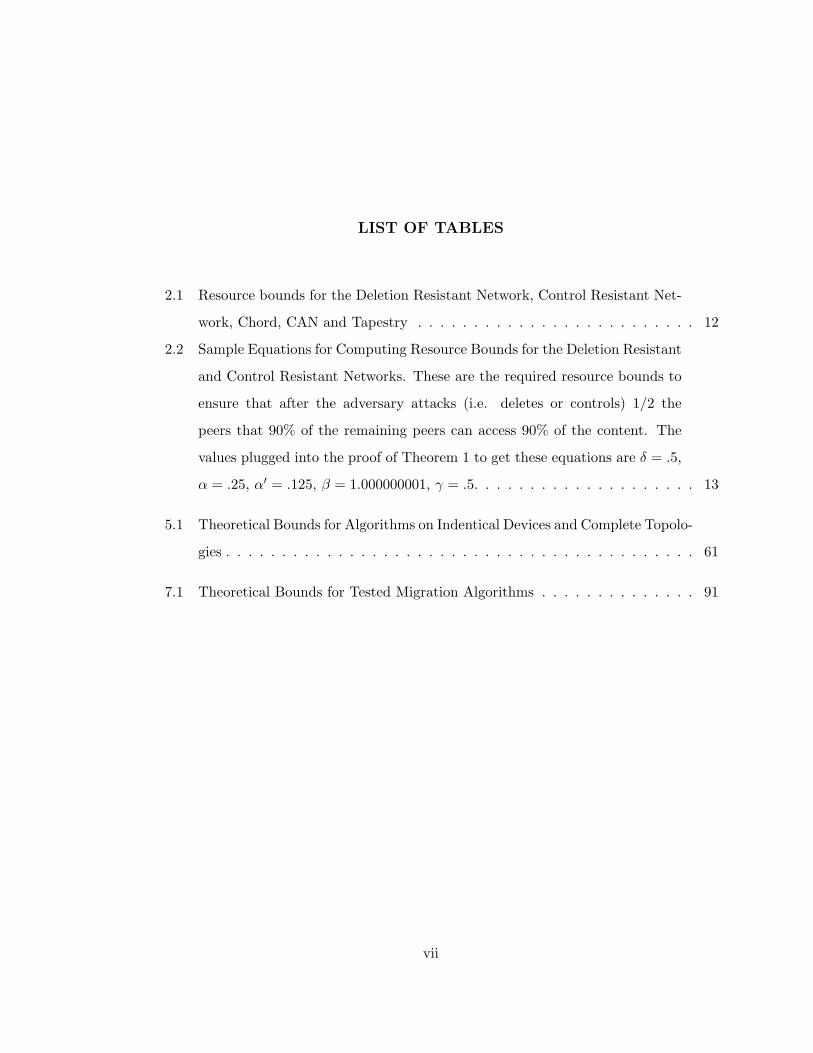
LIST OF TABLES
2.1 Resource bounds for the Deletion Resistant Network, Control Resistant Net-
work, Chord, CAN and Tapestry . . . . . . . . . . . . . . . . . . . . . . . . . 12
2.2 Sample Equations for Computing Resource Bounds for the Deletion Resistant
and Control Resistant Networks. These are the required resource bounds to
ensure that after the adversary attacks (i.e. deletes or controls) 1/2 the
peers that 90% of the remaining peers can access 90% of the content. The
values plugged into the proof of Theorem 1 to get these equations are δ = .5,
α = .25, α′ = .125, β = 1.000000001, γ = .5. . . . . . . . . . . . . . . . . . . . 13
5.1 Theoretical Bounds for Algorithms on Indentical Devices and Complete Topolo-
gies . . . . . . . . . . . . . . . . . . . . . . . . . . . . . . . . . . . . . . . . . . 61
7.1 Theoretical Bounds for Tested Migration Algorithms . . . . . . . . . . . . . . 91
vii
ACKNOWLEDGMENTS
Portions of this dissertation were previously published at SODA 2001 [HHK+01], SODA
2002 [FS02], WAE 2001 [AHH+01] and IPTPS 2002 [SFG+02]. The main overlaps are with
Chapter 3 (SODA 2002), Chapter 4 (IPTPS 2002), Chapter 6 (SODA 2001), and Chapter 7
(WAE 2001).
Many people have contributed to the research presented in this dissertation. First of all,
I would like to thank Anna Karlin and Amos Fiat for their encouragement, support and
mentoring in the past several years. Both Anna and Amos have taught me more than I can
say about the ins-and-outs of doing research in algorithms. Anna has patiently advised and
informed my taste in algorithmic problems, provided me with many wonderful problems
to work on, and given me the encouragement and advice I needed to succeed in solving
them. Amos has taught me how to define exciting algorithmic problems, how to maintain
a tenacity and flexibility when attacking problems, and how to write exciting and clear
theory papers. He has infected me with his incredible enthusiasm for practical algorithmic
problems.
Amos Fiat, Stefan Sariou, Steve Gribble, Anna Karlin and Prabhakar Raghavan con-
tributed greatly to the attack-resistance results presented in this thesis. All of the work on
attack-resistance is joint with Amos Fiat, who proposed the original idea of designing an
attack-resistant peer-to-peer network and provided constant encouragement and support.
His vision and contributions in this area were invaluable, these results would never have
been obtained without his collaboration. Stefan Sariou and Steve Gribble provided help-
ful information on the systems’ side of peer-to-peer networks and patiently answered our
simplistic questions. Anna Karlin provided useful feedback and Prabhakar Raghavan first
introduced me to the area of peer-to-peer networks.
Anna Karlin, Jason Hartline, Joe Hall, John Wilkes, Eric Anderson and Ram Swaminithan
viii
contributed to the data migration results discussed in this thesis. John Wilkes first pro-
posed the theoretical problems in data migration that are solved in this thesis. Anna and
Jason played a major role in obtaining the theoretical results discussed in Chapter 6. Joe
Hall, John Wilkes, Eric Anderson and Ram Swaminithan were instrumental in obtaining
the experimental results discussed in Chapter 7. Joe wrote the code used to do the experi-
ments, and John, Eric and Ram helped us in obtaining test cases, running experiments and
analyzing the results.
Finally, I would like to thank my partner, Julia Fitzsimmons, for her patience and
support throughout my graduate career. I hope to return the favor someday.
ix

1
Chapter 1
INTRODUCTION
The explosive growth of the Internet has created a high demand for access to vast
amounts of data. How to manage all of this data is an increasingly complicated problem.
Traditionally, management of data has been done in a centralized manner, but the last few
decades have witnessed a growing trend towards managing data in distributed systems.
Distributed systems are characterized by two main features. First they consist of mul-
tiple machines connected in a network. These machines may or may not all belong to the
same person or organization. Second, they present a unified user interface. In other words,
the users of the system are presented with the illusion that they are using a single, unified
computing facility. The first feature leads to many of the benefits of distributed systems in-
cluding: resource sharing, extensibility and fault-tolerance. These benefits make distributed
systems particularly adept at managing large amounts of data.
While distributed systems have characteristics which make them ideal for managing
large amounts of data, they also introduce many new problems when compared to central-
ized systems. In this thesis, we give algorithms for solving two important and essentially
independent problems related to distributed systems, the problems of attack-resistance and
data migration.
The rest of this chapter is organized as follows. In Section 1.1, we describe some of the
positive and negative characteristics of distributed systems and discuss the need for tradeoffs
when designing algorithms for such systems. In Section 1.2 , we provide motivation for the
problem of attack-resistance and in Section 1.3, we provide motivation for the problem of
data migration. In Section 1.4, we present the major contributions of this thesis. Finally in
Section 1.5, we outline the rest of the thesis.

2
1.1 Characteristics of Distributed Systems
The increasing popularity of distributed systems is due to many unique benefits they enjoy
over traditional centralized systems. These benefits include:
• Resource Sharing: The distributed system has access to all of the physical resources
of all the machines in the network. For example, all of the CPU power, disk space,
and network bandwidth of each machine is available to the system. Additionally, if
the machines in the system belong to different entities, then we can share all of the
content stored on the machines by the different entities.
• Extensibility: As the demand for service grows, we can simply add more machines
to the network. Each new machine brings more resources to the system. Thus the
performance of the entire distributed system can be much better than the performance
of a single centralized system.
• Fault Tolerance: There is no single point of failure for the distributed system, so
even if some machines go down, we may still be able to provide service. For example,
if we store copies of a data item on multiple machines, even if one machine fails, we
can still provide access to that data item.
• Anonymity: Since multiple machines participate in the system, it is possible to
access a data item without knowing exactly which machine stores that item.
Unfortunately, the benefits of distributed systems come at a cost. Following are some of
the problems faced by distributed systems when compared to centralized systems:
• Individual Machine Vulnerability: Multiple points of potential failure implies
greater likelihood of having at least one failure. Also, each machine in a distributed
system has limited resources to defend itself against an attack from outside. Finally,
the machines in the distributed system may not all be trustworthy.
3
• Load Balancing: In a distributed system, the responsibility for providing a service
is shared among multiple machines. How do we ensure that the tasks assigned to one
machine do not overwhelm the resources of that machine? For example, how do we
ensure that no single machine has responsibility for servicing requests for all of the
more popular data items?
• Time and Space Overhead: Data is frequently stored multiple times in the network
which increases space overhead. Also, commonly searching and updating data takes
more time than for a centralized system.
• Complexity: The problems of managing data in distributed systems are generally
much more complex than the problems of managing data in a centralized system.
This makes it harder to develop provably good algorithms for these problems, and the
algorithms developed tend to be more complex and thus harder to implement.
• Consistency: Distributed systems have the additional problem of maintaining the
consistency of data. In particular, if there are multiple copies of a data item in the
system, and one copy is changed, how should those changes be propogated to the
other copies?
1.1.1 Tradeoffs
Much of the work done in distributed systems involves tradeoffs, generally improving one
area is done at the expense of another. For example, one of the more important theoretical
results in distributed systems is the Byzantine generals algorithm [LSP82]. This algorithm
ensures consistency of state in the system (all non-faulty machines eventually store the
same value) at the cost of time overhead (the algorithm takes many stages to converge).
Another example is the work on weakly consistent replication done in the systems commu-
nity [PST+97, Sai]. This work improves the performance of the distributed systems at the
cost of weakening the consistency guarantees.
In this thesis, we address the problems of attack-resistance and data migration. To
do so, we will also be making similar tradeoffs. In our work on attack-resistance, we will

4
increase the fault-tolerance of the distributed system and the price we pay for this will be an
increase in the time and space overhead for the system: increased space for storing copies
of data items and increased time for operations like searching for data items. In our work
on data migration, we will give algorithms for solving load-balancing issues. The price we
pay for this will be increased time overhead for periodically moving data items around in
the network.
While our results do make necessary tradeoffs, we note that in many cases they do so in
the optimal or near optimal way. We further note that the tradeoffs made by our algorithms
generally increase the overall utility of the system. In the next two sections, we will motivate
the problems of attack-resistance and data migration. In Section 1.4, we will describe some
of the tradeoffs we make to solve these problems.
1.2 Motivation for Attack-Resistance
In this section, we motivate the problem of designing attack-resistant peer-to-peer networks.
A peer-to-peer (p2p) network is simply a distributed system for sharing data (e.g. music,
video, software, etc.) where each machine acts as both a server and a client. Peer-to-
peer(p2p) systems have enjoyed explosive growth recently, currently generating up to 70
percent of all traffic on the Internet [Gri02]. Perhaps the biggest reason for the popularity
of such systems is that they allow for the pooling of vast resources such as disk space, com-
putational power and bandwidth. Other reasons for their popularity include the potential
for anonymous storage of content and their robustness to random faults.
1.2.1 The Gnutella Network
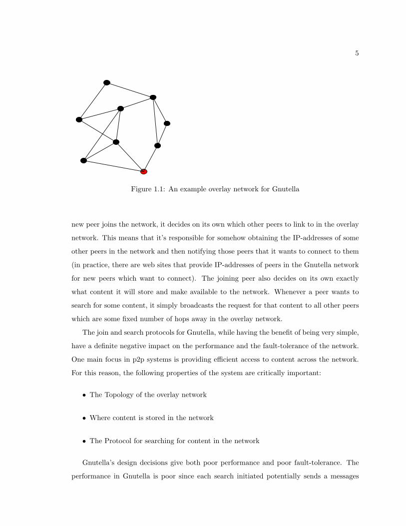
To better illustrate the nature of peer-to-peer systems, we will now describe the Gnutella [weba]
network, which is a simple but popular peer-to-peer system. Like all peer-to-peer systems,
Gnutella peers are connected in an overlay network. An overlay network is simply a vir-
tual network where a link from peer x to peer y means that x knows the IP-address of y
(Figure 1.2.1 gives an example overlay network for 9 peers).
The protocols for joining Gnutella and searching for content are very simple. When a
5
Figure 1.1: An example overlay network for Gnutella
new peer joins the network, it decides on its own which other peers to link to in the overlay
network. This means that it’s responsible for somehow obtaining the IP-addresses of some
other peers in the network and then notifying those peers that it wants to connect to them
(in practice, there are web sites that provide IP-addresses of peers in the Gnutella network
for new peers which want to connect). The joining peer also decides on its own exactly
what content it will store and make available to the network. Whenever a peer wants to
search for some content, it simply broadcasts the request for that content to all other peers
which are some fixed number of hops away in the overlay network.
The join and search protocols for Gnutella, while having the benefit of being very simple,
have a definite negative impact on the performance and the fault-tolerance of the network.
One main focus in p2p systems is providing efficient access to content across the network.
For this reason, the following properties of the system are critically important:
• The Topology of the overlay network
• Where content is stored in the network
• The Protocol for searching for content in the network
Gnutella’s design decisions give both poor performance and poor fault-tolerance. The
performance in Gnutella is poor since each search initiated potentially sends a messages

6
to every other peer in the network. This traffic overhead means that the network will not
scale well. The fault-tolerance of Gnutella is poor due to the ad hoc nature of the overlay
network and the content storage. For Gnutella in particular and for any p2p system in
general, design decisions have big implications for performance and fault-tolerance.
Many currently deployed peer-to-peer systems have poor performance, which impacts
the efficiency and scalability of the system. No currently deployed systems have both good
performance and attack-resistance. In this thesis, we give the first p2p system which has
both attack resistance and good performance.
1.2.2 Why is Attack-Resistance Important?
Web content is under attack by states, corporations, and malicious agents. States and corpo-
rations have repeatedly censored content for political and economic reasons [Fou, oC, Mar].
This censorship has been both for copyright infringement (e.g. Napster) and for political
reasons (e.g. China’s net censorship). Additionally, denial-of-service attacks launched by
malicious agents are highly prevalent on the web, targeting a wide-range of victims [Dav01].
Peer-to-peer systems are particular vulnerable to attack since a single peer lacks the tech-
nical and legal resources with which to defend itself against attack.
Current p2p systems are not attack-resistant. The most famous evidence for this is
Napster [webb] which has been effectively dismembered by legal attacks on the central server.
Additionally, Gnutella ([weba]), while was specifically designed to avoid the vulnerability
of a central server, is highly vulnerable to attack by removing a very small number of
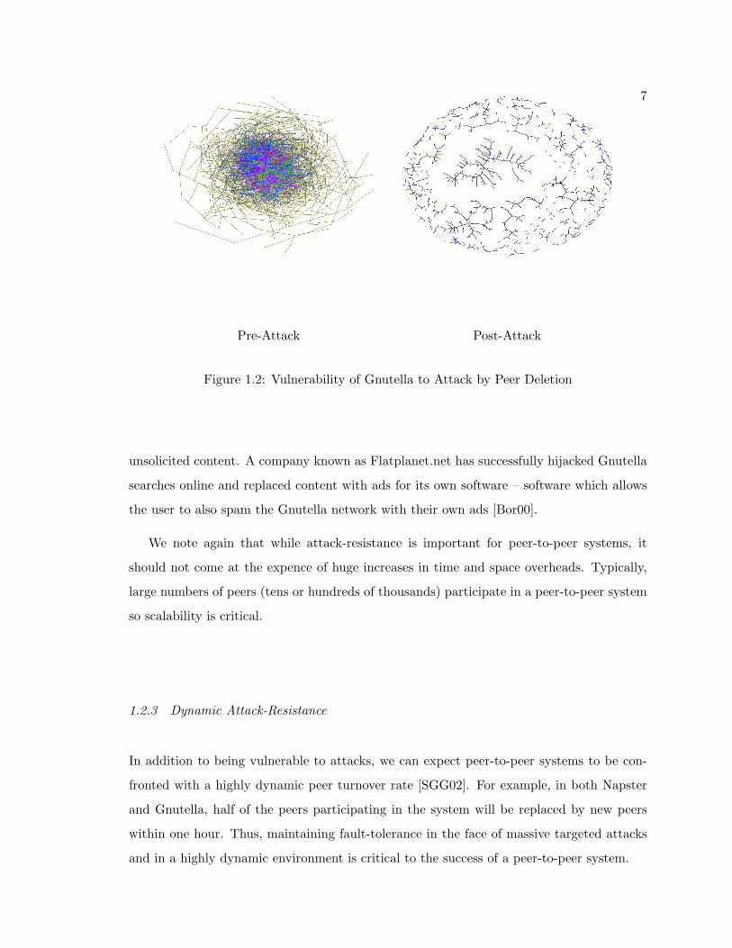
carefully chosen nodes. The vulnerability of Gnutella is illustrated in Figure 1.2.2 taken
from [SGG02]. The left part of this figure is a snapshot of an overlay network in Gnutella
taken in February, 2001 [SGG02] consisting of 1771 peers. The right part of the figure
shows the same network after deleting 63 of the most highly connected peers. Effectively
the overlay network has been shattered into a large number of small connected components
by removing a very small number of carefully chosen peers. In addition to vulnerability to
attack by peer deletion, Gnutella is also vulnerable to attack by peers trying to “spam” the
network. Malicious peers “spam” the network by responding to queries on the network with
7
Pre-Attack Post-Attack
Figure 1.2: Vulnerability of Gnutella to Attack by Peer Deletion
unsolicited content. A company known as Flatplanet.net has successfully hijacked Gnutella
searches online and replaced content with ads for its own software – software which allows
the user to also spam the Gnutella network with their own ads [Bor00].
We note again that while attack-resistance is important for peer-to-peer systems, it
should not come at the expence of huge increases in time and space overheads. Typically,
large numbers of peers (tens or hundreds of thousands) participate in a peer-to-peer system
so scalability is critical.
1.2.3 Dynamic Attack-Resistance
In addition to being vulnerable to attacks, we can expect peer-to-peer systems to be con-
fronted with a highly dynamic peer turnover rate [SGG02]. For example, in both Napster
and Gnutella, half of the peers participating in the system will be replaced by new peers
within one hour. Thus, maintaining fault-tolerance in the face of massive targeted attacks
and in a highly dynamic environment is critical to the success of a peer-to-peer system.

8
1.3 Motivation for Data Migration
In this section, we motivate the second major problem addressed in this thesis: data mi-
gration. While distributed systems have many benefits over centralized systems, they also
introduce new problems. As we have suggested, the performance of these systems depends
critically on load-balancing: we must have an assignment of data to machines that balances
the load across machines as evenly as possible. Unfortunately, the optimal data layout is
likely to change over time, for example, when either the user workloads change, when new
machines are added to the system, or when existing machines go down. Consequently, it is
common to periodically compute a new optimal (or at least very good) assignment of data
to devices based on newly predicted workloads and machine specifications (such as speed
and storage capacity) [BGM+97, GS90, GSKTZ00, Wol89]. Once the new assignment is
computed, the data must be migrated from its old configuration to its new configuration.
For many modern distributed distributed systems, the administration typically follows
an iterative loop consisting of the following three tasks [AHK+01]:
• Analyzing the data request patterns to determine the load on each of the storage
devices;
• Computing a new configuration of data on the devices which better balances the loads;
• Migrating the data from the current configuration to the new configuration.
The last task in this loop is the data migration problem. In this thesis, we will focus solely
on this step of the loop as the first two steps have been addressed in previous work[AHK+01]
. It’s critically important to perform the data migration as quickly as possible, since during
the time the migration is being performed, the system is running suboptimally.
1.4 Contributions
In this thesis, we show that we can design provably good algorithms for the real-world
problems of attack-resistance and data migration. In particular, our contributions are as
follows:
9
• Attack Resistance: We describe the first fully distributed, scalable, attack-resistant
peer-to-peer network. The network is attack-resistant in the sense that even when a
constant fraction of the nodes in the network are deleted or controlled by an adversary,
an arbitrarily large fraction of the remaining nodes can access an arbitrarily large
fraction of the data items. Furthermore, the network is scalable in the sense that time
and space resource bounds grow poly-logarithmically with the number of nodes in
the network. We also describe a scalable peer-to-peer network that is attack-resistant
in a highly dynamic environment: the network remains robust even after all of the
original nodes in the network have been deleted by the adversary, provided that a
larger number of new nodes have joined the network.
• Data Migration: The data migration problem is the problem of computing an effi-
cient plan for moving data stored on machines in a network from one configuration to
another. We first consider the case where the network topology is complete and all
machines have the same transfer speeds. For this case, we describe polynomial time
algorithms for finding a near-optimal migration plan when a certain number of addi-
tional nodes is available as temporary storage (the plan is near-optimal in the sense
that it is essentially the fastest plan possible). We also describe a 3/2-approximation
algorithm for the case where such nodes are not available. We empirically evaluate our
algorithms for this problem and find they perform much better in practice than the
theoretical bounds suggest. Finally, we describe several provably good algorithms for
the more difficult case where the network topology is not complete and where machine
speeds are variable.
1.5 Thesis Map
The rest of this thesis is structured as follows. Chapter 2 describes our theoretical results
on attack-resistant peer-to-peer networks along with related work. Chapters 3 and 4 gives
the algorithms which achieve these results along with proofs of correctness. Chapter 5 de-
scribes our problem formulations and theoretical and empirical results on the data migration
problem along with related work. Chapters 6 and 8 give the algorithms which achieve the

10
theoretical results along with proofs of correctness while Chapter 7 gives the detailed em-
pirical results. Chapter 9 outlines directions for future work and concludes with a summary
of our major contributions.
11
Chapter 2
INTRODUCTION TO ATTACK-RESISTANT PEER-TO-PEER
SYSTEMS
In this chapter, we describe our results for attack-resistant peer-to-peer networks. In
Section 2.1 we describe the results for the Deletion Resistant Network, the Control Resistant
Network and the Dynamically Attack-Resistant Network. In Section 2.2, we describe related
work.
2.1 Our Results
2.1.1 Our Assumptions
In all of our results on attack-resistant networks, we assume a synchronous model of com-
munication. In other words, we assume that there is some fixed amount of time that it takes
to send a message from one peer in the network to another peer and that all peers know
this time bound. In practice, all peers can assume a time bound which is say ten times the
average link latency. The number of neighboring peers which have latencies greater than
this will be a very small fraction of all peers and, in our analysis, these peers can be included
among the peers successfully attacked by the adversary.
In all of our results, we will assume that faults are adversarial. In contrast to independent
faults, adversarial faults can be targetted at certain important peers. Thus, adversarial
faults are strictly worse than independent faults. Finally, we note that our attack-resistant
networks, in addition to tolerating node failures, can also tolerate communication failures
like network partitions.
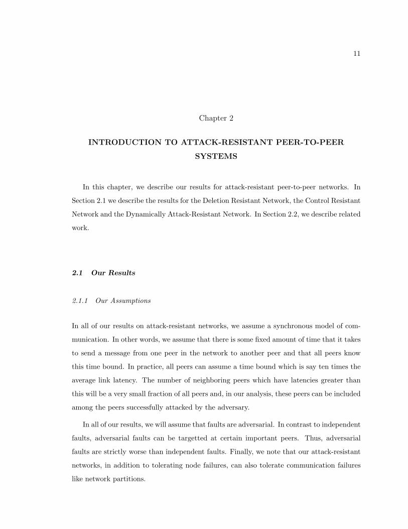
12
Table 2.1: Resource bounds for the Deletion Resistant Network, Control Resistant Network,Chord, CAN and Tapestry
Network Storage Search Search Deletion Control
Per Peer Time Messages Resistant? Resistant?
Deletion Resistant Network O(log n) O(log n) O(log2 n) Yes No
Control Resistant Network O(log2 n) O(log n) O(log3 n) Yes Yes
Dynamically Resistant Network O(log3 n) O(log n) O(log3 n) Yes Yes
Chord [SMK+01] O(log n) O(log n) O(log n) No No
CAN [RFH+01] O(log n) O(log n) O(log n) No No
Tapestry [ZKJ01] O(log n) O(log n) O(log n) No No
2.1.2 Theoretical Results
Below we give the technical results for our attack-resistant networks. The technical descrip-
tion of the the deletion resistant and control resistant networks are found in Chapter 3.
Chapter 4 describes the dynamically attack-resistant network. Summaries of our results for
the deletion and control resistant networks are given in Table 2.1. These results assume
a network of n peers storing O(n) data items. For comparison, we have included in this
table results for other peer-to-peer networks in the literature. (These other networks are
described in Section 2.2).
2.1.3 The Constants
Some exact equations for resource bounds for the Deletion Resistant Network and the Con-
trol Resistant Network are given in Table 2.2. These resource bounds are for the case where
we guarantee that after the adversary attacks (deletes or controls) half the peers, 90% of
the remaining peers can access 90% of the content. Solving for the optimal constants in
these equations is NP-Hard so the equations reported have non-optimal constants.
The constants in these equations show that the results for the Deletion Resistant and
Control Resistant Networks are still far from being practical for any reasonably small values

13
Table 2.2: Sample Equations for Computing Resource Bounds for the Deletion Resistantand Control Resistant Networks. These are the required resource bounds to ensure thatafter the adversary attacks (i.e. deletes or controls) 1/2 the peers that 90% of the remainingpeers can access 90% of the content. The values plugged into the proof of Theorem 1 to getthese equations are δ = .5, α = .25, α′ = .125, β = 1.000000001, γ = .5.
Deletion Resistant Network Control Resistant Network
Space Per Peer 19, 246 ∗ lnn + 18, 060 32, 620 ∗ ln2 n + 7
Hops Per Search 7 log n 7 log n
Messages Per Search 394, 000 ∗ ln2 n 1, 425, 115 ∗ ln3 n
of n. In particular, the number of peers in Gnutella now is around 100, 000 and the number of
users of the internet is about 100, 000, 000. Unfortunately, even for a network of 100, 000, 000
peers, the number of messages sent per search in both the Deletion Resistant and Control
Resistant Networks would exceed the total number of peers in the network (and thus our
search algorithms would compare unfavorably with a naive broadcast algorithm). Hence
our results are primarily of theoretical interest.
To be fair, we note that our bias in constructing these networks and proofs was towards
simplifing the mathematical analysis rather than minimizing the constants. It is possible
that the constants could be significantly reduced with somewhat different algorithms and
proof techniques.
2.1.4 Deletion Resistant Network
In Chapter 3, we present a peer-to-peer network with n nodes used to store n distinct data
items1. As far as we know this is the first such scheme of its kind. The scheme is robust
to adversarial deletion of up to2 half of the nodes in the network and has the following
properties:
1For simplicity, we’ve assumed that the number of items and the number of nodes is equal. However, forany n nodes and m ≥ n data items, our scheme will work, where the search time remains O(log n), thenumber of messages remains O(log2 n), and the storage requirements are O((m/n) log n) per node.
2For simplicity, we give the proofs with this constant equal to 1/2. However we can easily modify thescheme to work for any constant less than 1. This would change the constants involved in storage, searchtime, and messages sent, by a constant factor.

14
1. With high probability, all but an arbitrarily small fraction of the nodes can find all
but an arbitrarily small fraction of the data items.
2. Search takes (parallel) time O(log n).
3. Search requires O(log2 n) messages in total.
4. Every node requires O(log n) storage.
For reasons enumerated in the Introduction, in the context of peer-to-peer systems, it
seems important to consider adversarial attacks rather than random deletion. Our scheme
is robust against adversarial deletion.
We remark that such a network is clearly resilient to having up to 1/2 of the nodes
removed at random, (in actuality, its random removal resiliency is much better). We further
remark that if nodes come up and down over time, our network will continue to operate as
required so long as at least n/2 of the nodes are alive.
2.1.5 Control Resistant Network
In Chapter 3, we also present our control resistant network. This is a variant of the deletion
resistant network which is resistant to an adversary which controls the peers it attacks
rather than deletes them. To the best of our knowledge this is the first such scheme of its
kind. As before, assume n nodes used to store n distinct data items. The adversary may
choose up to some constant c < 1/2 fraction of the nodes in the network. These nodes
under adversary control may be deleted, or they may collude and transmit arbitrary false
versions of the data item, nonetheless:
1. With high probability, all but an arbitrarily small fraction of the nodes will be able
to obtain all but an arbitrarily small fraction of the true data items. To clarify this
point, the search will not result in multiple items, one of which is the correct item.
The search will result in one unequivocal true item.
2. Search takes (parallel) time O(log n).
15
3. Search requires O(log3 n) messages in total.
4. Every node requires O(log2 n) storage.
2.1.6 Dynamically Attack-Resistant Network
In Chapter 4, we describe the dynamically attack-resistant network. This network is robust
even when all of the original peers in the network are deleted provided that enough new
peers join the network. For this result, we assume that we start with a network of n peers
for some fixed n, that the number of data items stored is always O(n), and that each joining
peer knows one random peer.
We say an adversary is (γ, δ)-limited if for some γ > 0, δ > γ, at least δn peers join the
network in any time interval when adversary deletes γn peers.
We say a peer-to-peer network is ε-robust at some particular time if all but an ε fraction
of the peers can access all but an ε fraction of the content.
Finally we say a peer-to-peer network is ε-dynamically attack-resistant if, with high
probability, the network is always ε-robust during any period when a limited adversary
deletes a number of peers polynomial in n.
Our main result is the following: For any ε > 0, γ < 1 and δ > γ + ε, we give a
ε-dynamically attack-resistant network such that:
• the network is ε-robust assuming δn peers added whenever γn peers deleted.
• Search takes O(log n) time and O(log3 n) messages
• Every peer maintains pointers to O(log3 n) other peers
• Every peer stores O(log n) data items
• Peer insertion takes O(log n) time
16
2.2 Related Work
2.2.1 Peer-to-peer Networks (not Content Addressable)
Peer-to-peer networks are a relatively recent and quickly growing phenomena. The average
number of Gnutella users in any given day is no less than 10, 000 and may range as high as
30, 000 [Cli]. Napster software has been downloaded by 50 million users [RFH+01]. There
are a wide range of popular deployed peer-to-peer systems including: Napster, Gnutella,
Morpheus, Kazaa, Audiogalaxy, iMesh, Madster, FreeNet, Publius, Freehaven, NetBatch,
MBone, Groove, NextPage, Reptile and Yaga. Due to naive algorithms for searching for con-
tent, many of these deployed peer-to-peer systems are not scalable. For example, Gnutella
requires up to O(n) messages for a search (search is performed via a general broadcast),
this has effectively limited the size of Gnutella networks to about 1000 nodes [Cli].
Pandurangam, Raghavan, and Upfal [PRU01] address the problem of maintaining a
connected network under a probabilistic model of node arrival and departure. They do
not deal with the question of searching within the network. They give a protocol which
maintains a network on n nodes with diameter O(log n). The protocol requires constant
memory per node and a central hub with constant memory with which all nodes can connect.
Experimental measurements of a connected component of the real Gnutella network have
been studied [SGG02], and it has been found to still contain a large connected component
even with a 1/3 fraction of random node deletions.
2.2.2 Content Addressable Networks — Random Faults
A more principled approach than the naive approach taken by many deployed systems is
the use of a content addressable network (CAN) [RFH+01]. A content addressable network
is defined as a distributed, scalable, indexing scheme for peer-to-peer networks.
There are several papers that address the problem of creating a content addressable
network. Plaxton, Rajaram and Richa [PRR97] give a context addressable network for web
caching. Search time and the total number of messages is O(log n), and storage requirements
are O(log n) per node.
Tapestry [ZKJ01] is an extension to the [PRR97] mechanism, designed to be robust
17
against faults. It is used in the Oceanstore [KBC+00] system. Experimental evidence is
supplied that Tapestry is robust against random faults.
Ratnasamy et. al. [RFH+01] describe a system called CAN which has the topology of a
d-dimensional torus. As a function of d, storage requirements are O(d) per node, whereas
search time and the total number of messages is O(dn1/d). There is experimental evidence
that CAN is robust to random faults.
Finally, Stoica et. al. introduce yet another content addressable network, Chord
[SMK+01], which, like [PRU01] and [ZKJ01], requires O(log n) memory per node and
O(log n) search time. Chord is provably robust to a constant fraction of random node
failures.
It is unclear whether it is possible to extend any of these systems to remain robust
under orchestrated attacks. In addition, many known network topologies are known to be
vulnerable to adversarial deletions. For example, with a linear number of node deletions,
the hypercube can be fragmented into components all of which have size no more than
O(n/√
log n) ([HLN89]).
2.2.3 Faults on Networks
Random Faults
There is a large body of work on node and edge faults that occur independently at random
in a general network. Hastad, Leighton and Newman [HLN89] address the problem of
routing when there are node and edge faults on the hypercube which occur independently
at random with some probability p < 1. They give a O(log n) step routing algorithm that
ensures the delivery of messages with high probability even when a constant fraction of
the nodes and edges have failed. They also show that a faulty hypercube can emulate a
fault-free hypercube with only constant slowdown.
Karlin, Nelson and Tamaki [KNT94] explore the fault tolerance of the butterfly network
against edge faults that occur independently at random with probability p. They show
that there is a critical probability p∗ such that if p is less than p∗, the faulted butterfly
almost surely contains a linear-sized component and that if p is greater than p∗, the faulted

18
butterfly does not contain a linear sized component.
Leighton, Maggs and Sitamaran [LMS98] show that a butterfly network whose nodes
fail with some constant probability p can emulate a fault-free network of the same size with
a slowdown of 2O(log∗ n).
Adversarial Faults
It is well known that many common network topologies are not resistant to a linear number
of adversarial faults. With a linear number of faults, the hypercube can be fragmented into
components all of which have size no more than O(n/√
log n) [HLN89]. The best known
lower bound on the number of adversarial faults a hypercube can tolerate and still be able
to emulate a fault free hypercube of the same size is O(log n) [HLN89].
Leighton, Maggs and Sitamaran [LMS98] analyze the fault tolerance of several bounded
degree networks. One of their results is that any n node butterfly network containing n1−ε
(for any constant ε > 0) faults can emulate a fault free butterfly network of the same size
with only constant slowdown. The same result is given for the shuffle-exchange network.
2.2.4 Other Theoretical Related Work
One attempt at censorship resistant web publishing is the Publius system [MWC00], while
this system has many desirable properties, it is not a peer-to-peer network. Publius makes
use of many cryptographic elements and uses Shamir’s threshold secret sharing scheme
[Sha79] to split the shares amongst many servers. When viewed as a peer-to-peer network,
with n nodes and n data items, to be resistant to n/2 adversarial node removals, Publius
requires Ω(n) storage per node and Ω(n) search time per query.
Alon et al. [AKK+00] give a method which safely stores a document in a decentralized
storage setting where up to half the storage devices may be faulty. The application context
of their work is a storage system consisting of a set of servers and a set of clients where each
client can communicate with all the servers. Their scheme involves distributing specially
encoded pieces of the document to all the servers in the network.
Aumann and Bender [AB96] consider tolerance of pointer-based data structures to worse

19
case memory failures. They present fault tolerant variants of stacks, lists and trees. They
give a fault tolerant tree with the property that if r adversarial faults occur, no more than
O(r) of the data in the tree is lost. This fault tolerant tree is based on the use of expander
graphs.
Quorum systems [Gif79, MRW00, MRWW98] are an efficient, robust way to read and
write to a variable which is shared among n servers. Many of these systems are resistant
up to some number b < n/4 of Byzantine faults. The key idea in such systems is to create
subsets of the servers called quorums in such a way that any two quorums contain at least
2b+1 servers in common. A client that wants to write to the shared variable will broadcast
the new value to all servers in some quorum. A client that wants to read the variable will
get values from all members in some quorum and will keep only that value which has the
most recent time stamp and is returned by at least b + 1 servers. For quorum systems that
are resistant to θ(n) faults the load on the servers can be high. In particular, θ(n) servers
will be involved in a constant fraction of the queries.
Recently Malkhi et. al. [MRWW98] have introduced a probabilistic quorum system.
This new system relaxes the constraint that there must be 2b + 1 servers shared between
any two quorums and remains resistant to Byzantine faults only with high probability. The
load on servers in the probabilistic system is less than the load in the deterministic system.
Nonetheless, for a probabilistic quorum system which is resistant to θ(n) faults, there still
will be at least one server involved in a constant fraction of the queries.
2.2.5 Other Empirical Related Work
There are several major systems projects which address the problem of maintaining avail-
ability of published files in the face of attacks. In this section, we explore two of these
systems: Eternity and Farsite. Eternity [And96] is a file sharing system designed to be
resistant to both denial-of-service and legal attacks. The system seeks to ensure that a
file, once published in the system, always remains available to all users. In other words,
the file can not be removed or changed even by the publisher of that file. Replication is
used to ensure availability of files and cryptographic tools are used to ensure that file lo-
20
cation information is inacessible. The system achieves resistance to attack primarily by
this inacessibility of file location information. Search for a file in the worst case is done
by broadcasting to all users in the network. In contrast to the Eternity system, in our
attack-resistant networks, the locations of all files are known to all peers and search is not
done by broadcast.
Farsite [BDET00] is an architecture for a serverless distributed file system in an envi-
ronment where not all clients are trusted. Farsite also uses replication and cryptographic
techniques to achieve reliability and data integrity in an untrusted environment. Signifi-
cant empirical evidence is provided to show that Farsite has good time and space resource
bounds. However, while empirical evidence is provided to suggest that Farsite provides good
reliability in the face of typical machine faults, there is no empirical or theoretical evidence
that the system is robust to adversarial faults.
21
Chapter 3
THE DELETION RESISTANT AND CONTROL RESISTANT
NETWORKS
In this chapter, we describe the deletion and content resistant networks in detail and
provide proofs of their attack-resistance and good performance. We give the algorithm for
creation of our deletion resistant network, the search mechanism, and the attack-resistant
properties in Section 3.1. The proof of our main theorem for the deletion resistant network,
Theorem 1, is given in Section 3.2. In Section 3.3 we sketch the modifications required in
the algorithms and the proofs to obtain the control resistant network. The main theorem
with regard to the control resistant network is Theorem 19.
3.1 The Deletion Resistant Network
In this section, we state our mechanism for providing indexing of n data items by n nodes
in a network that is robust to adversarial removal of half of the nodes. We make use of a
n-node butterfly network of depth log n − log log n.
We call the nodes of the butterfly network supernodes (see Figure 1). Every supernode
is associated with a set of O(log n)peers and every peer is in O(log n) supernodes. We call
a supernode at the topmost level of the butterfly a top supernode, one at the bottommost
level of the network a bottom supernode and one at neither the topmost or bottommost
level a middle supernode.
To construct the network we do the following:
• We choose an error parameter ε > 0, and as a function of ε we determine constants
C, B, T , D, α and β. (See Theorem 1).
• Every peer chooses at random C top supernodes, C bottom supernodes and C log n
middle supernodes to which it will belong.
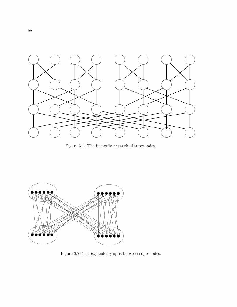
22
Figure 3.1: The butterfly network of supernodes.
Figure 3.2: The expander graphs between supernodes.
23
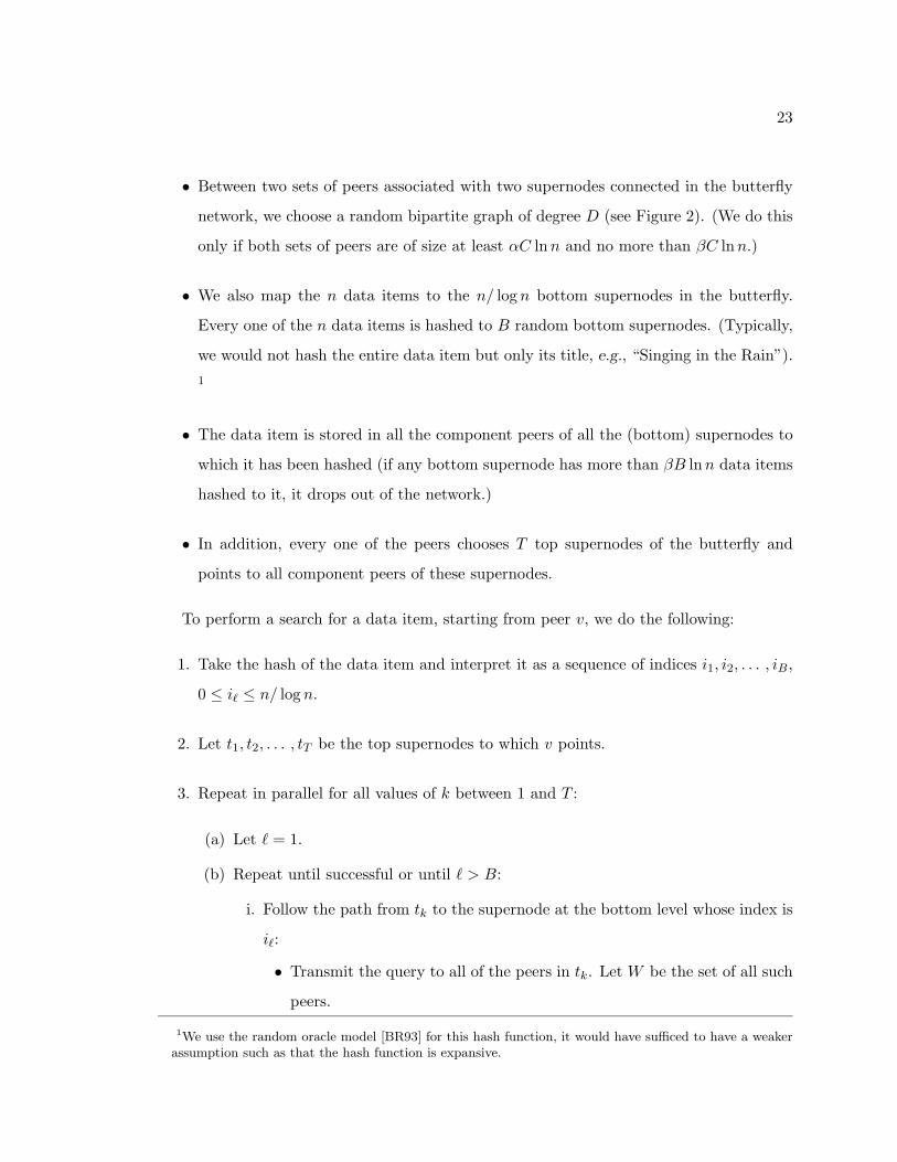
• Between two sets of peers associated with two supernodes connected in the butterfly
network, we choose a random bipartite graph of degree D (see Figure 2). (We do this
only if both sets of peers are of size at least αC lnn and no more than βC lnn.)
• We also map the n data items to the n/ log n bottom supernodes in the butterfly.
Every one of the n data items is hashed to B random bottom supernodes. (Typically,
we would not hash the entire data item but only its title, e.g., “Singing in the Rain”).1
• The data item is stored in all the component peers of all the (bottom) supernodes to
which it has been hashed (if any bottom supernode has more than βB lnn data items
hashed to it, it drops out of the network.)
• In addition, every one of the peers chooses T top supernodes of the butterfly and
points to all component peers of these supernodes.
To perform a search for a data item, starting from peer v, we do the following:
1. Take the hash of the data item and interpret it as a sequence of indices i1, i2, . . . , iB,
0 ≤ i ≤ n/ log n.
2. Let t1, t2, . . . , tT be the top supernodes to which v points.
3. Repeat in parallel for all values of k between 1 and T :
(a) Let = 1.
(b) Repeat until successful or until > B:
i. Follow the path from tk to the supernode at the bottom level whose index is
i:
• Transmit the query to all of the peers in tk. Let W be the set of all such
peers.
1We use the random oracle model [BR93] for this hash function, it would have sufficed to have a weakerassumption such as that the hash function is expansive.

24
• Repeat until a bottom supernode is reached:
– The peers in W transmit the query to all of their neighbors along the
(unique) butterfly path to i, Let W be this new set of peers.
• When the bottom supernode is reached, fetch the content from whatever
peer has been reached.
• The content, if found, is transmitted back along the same path as the
query was transmitted downwards.
ii. Increment .
3.1.1 Properties of the Deletion Resistant Network
Following is the main theorem which we will prove in Section 3.2.
Theorem 1 For all ε > 0, there exist constants k1(ε), k2(ε), k3(ε) which depend only on ε
such that
• Every peer requires k1(ε) log n memory.
• Search for a data item takes no more than k2(ε) log n time.
• Search for a data item requires no more than k3(ε) log2 n messages.
• All but εn peers can reach all but εn data items after deletion of any half of the peers.
3.1.2 Some Comments
1. Distributed creation of the content addressable network
We note that our Content Addressable Memory can be created in a fully distributed
fashion with n broadcasts or transmission of n2 messages in total and assuming
O(log n) memory per peer. We briefly sketch the protocol that a particular peer
will follow to do this. The peer first randomly chooses the supernodes to which it
belongs. Let S be the set of supernodes which neighbor supernodes to which the peer
belongs. For each s ∈ S, the peer chooses a set Ns of D random numbers between 1
25
and βC lnn. The peer then broadcasts a message to all other peers which contains
the identifiers of the supernodes to which the peer belongs.
Next, the peer will receive messages from all other peers giving the supernodes to
which they belong. For every s ∈ S, the peer will link to the i-th peer that belongs
to s from which it receives a message if and only if i ∈ Ns.
If for some supernode to which the peer belongs, the peer receives less than αC lnn or
greater than βC lnn messages from other peers in that supernode, the peer removes all
out-going connections associated with that supernode. Similarly, if for some supernode
in S, the peer receives less than αC lnn or greater than βC lnn messages from other
peers in that supernode, the peer removes all out-going connections to that neighboring
supernode. Connections to the top supernodes and storage of data items can be
handled in a similar manner.
2. Insertion of a New Data Item
One can insert a new data item simply by performing a search, and sending the
data item along with the search. The data item will be stored at the peers of the
bottommost supernodes in the search. We remark that such an insertion may fail
with some small constant probability.
3. Insertion of a New Peer
Our network does not have an explicit mechanism for peer insertion. It does seem
that one could insert the peer by having the peer choose at random appropriate
supernodes and then forge the required random connections with the peers that belong
to neighboring supernodes. The technical difficulty with proving results about this
insertion process is that not all live peers in these neighboring supernodes may be
reachable and thus the probability distributions become skewed.
We note though that a new peer can simply copy the links to top supernodes of some
other peer already in the network and will thus very likely be able to access almost
all of the data items. This insertion takes O(log n) time. Of course the new peer will

26
not increase the resiliency of the network if it inserts itself in this way. We assume
that a full reorganization of the network is scheduled whenever sufficiently many new
peers have been added in this way.
4. Load Balancing Properties
Because the data items are searched for along a path from a random top supernode
to the bottom supernodes containing the item, and because these bottom supernodes
are chosen at random, the load will be well balanced as long as the number of requests
for different data items is itself balanced. This follows because a uniform distribution
on the search for data items translates to a uniform distribution on top to bottom
paths through the butterfly.
3.2 Proofs
In this section, we present the proof of Theorem 1 which is the main result of this chapter.
3.2.1 Proof Overview
Technically, the proof makes extensive use of random constructions and the Probabilistic
Method [AS00].
We first show that with high probability, all but an arbitrarily small constant times
n/ log n of the supernodes are good, where good means that (a) they have O(log n) peers
associated with them, and, (b) they have Ω(log n) live peers after adversarial deletion. We
note that the first property gives an upper bound on the number of pointers any peer must
store. The second property implies that after attack, all but a small constant fraction of
the paths through the butterfly contain only good supernodes.
Search is preformed by broadcasting the search to all the peers in (a constant number
of) top supernodes, followed by a sequence of broadcasts between every successive pair of
supernodes along the paths between one of these top supernodes and a constant number of
bottom supernodes. Fix one such path. The broadcast between two successive supernodes
along the path makes use of the expander graph connecting these two supernodes. When

27
Supernode Supernode Supernode
LiveNodes
DeadNodes
LiveNodes
DeadNodes
Figure 3.3: Traversal of a path through the butterfly.
we broadcast from the live peers in a supernode to the following supernode, the peers that
we reach may be both live and dead(see Figure 3).
Assume that we broadcast along a path, all of whose supernodes are good. One problem
is that we are not guaranteed to reach all the live peers in the next supernode along the
path. Instead, we reduce our requirements to ensure that at every stage, we reach at least
δ log n live peers, for some constant δ. The crucial observation is that if we broadcast from
δ log n live peers in one supernode, we are guaranteed to reach at least δ log n live peers
in the subsequent supernode, with high probability. This follows by using the expansion
properties of the bipartite expander connection between two successive supernodes.
Recall that the peers are connected to a constant number of random top supernodes,
and that the data items are stored in a constant number of random bottom supernodes.
The fact that we can broadcast along all but an arbitrarily small fraction of the paths in
the butterfly implies that most of the peers can reach most of the content.
In several statements of the lemmata and theorems in this section, we require that n,
the number of peers in the network, be sufficiently large to get our result. We note that,
technically, this requirement is not necessary since if it fails then n is a constant and our
claims trivially hold.

28
3.2.2 Technical Lemmata
Following are three technical lemmata about bipartite expanders that we will use in our
proofs. The proof of the first lemma is well known [Pin73] (see also [MR95]) and the proof
of the next two lemmata are slight variants on the proof of the first. The proofs of all three
lemmata are included in Section 3.4 for completeness.
Lemma 2 Let l, r, l′, r′, d and n be any positive values where l′ ≤ l and r′ ≤ r and
d ≥ r
r′l′
(l′ ln
(le
l′
)+ r′ ln
(re
r′
)+ 2 lnn
).
Let G be a random bipartite multigraph with left side L and right side R where |L| = l and
|R| = r and each peer in L has edges to d random neighbors in R. Then with probability at
least 1 − 1/n2, any subset of L of size l′ shares an edge with any subset of R of size r′ .
Lemma 3 Let l, r, l′, r′, d, λ and n be any positive values where l′ ≤ l, r′ ≤ r, 0 < λ < 1
and
d ≥ 2r
r′l′(1 − λ)2
(l′ ln
(le
l′
)+ r′ ln
(re
r′
)+ 2 lnn
).
Let G be a random bipartite multigraph with left side L and right side R where |L| = l and
|R| = r and each peer in L has edges to d random neighbors in R. Then with probability at
least 1 − 1/n2, for any set L′ ⊂ L where |L′| = l′, there is no set R′ ⊂ R, where |R′| = r′
such that all peers in R′ share less than λl′d/r edges with L′.
Lemma 4 Let l, r, r′, d, β′ and n be any positive values where l′ ≤ l, β′ > 1 and
d ≥ 4r
r′l(β′ − 1)2(r′ ln
(re
r′
)+ 2 lnn
).
Let G be a random bipartite multigraph with left side L and right side R where |L| = l and
|R| = r and each peer in L has edges to d random neighbors in R. Then with probability at
least 1 − 1/n2, there is no set R′ ⊂ R, where |R′| = r′ such that all peers in R′ have degree
greater than β′ld/r.

29
3.2.3 Definitions
Definition 5 A top or middle supernode is said to be (α, β)-good if it has at most β log n
peers mapped to it and at least α log n peers which are not under control of the adversary.
Definition 6 A bottom supernode is said to be (α, β)-good if it has at most β log n peers
mapped to it and at least α log n peers which are not under control of the adversary and if
there are no more than βB lnn data items that map to the peer.
Definition 7 An (α, β)-good path is a path through the butterfly network from a top su-
pernode to a bottom supernode all of whose supernodes are (α, β)-good supernodes.
Definition 8 A top supernode is called (γ, α, β)-expansive if there exist γn/ log n (α, β)-
good paths that start at this supernode.
3.2.4 (α, β)-good Supernodes
Lemma 9 Let α, δ′, n be values where α < 1/2 and δ′ > 0 and let k(δ′, α) be a value
that depends only on α, δ′ and assume n is sufficiently large. Let each peer participate in
k(δ′, α) ln n random middle supernodes. Then removing any set of n/2 peers still leaves all
but δ′n/ lnn middle supernodes with at least αk(δ′, α) ln n live peers.
Proof: For simplicity, we will assume there are n middle supernodes (we can throw out
any excess supernodes).
Let l = n, l′ = n/2, r = n, r′ = δ′n/ lnn, λ = 2α and d = k(δ′, α) ln n in Lemma 3.
We want probability less than 1/n2 of being able to remove n/2 peers and having a set of
δ′n/ lnn supernodes all with less than αk(δ′, α) ln n live peers. This happens provided that
the number of connections from each supernode is bounded as in Lemma 3:
k(δ′, α) ln n ≥ 4 lnn
δ′n(1 − 2α)2
(n ln(2e)
2+
δ′n
ln n· ln
(lnn
δ′
)+ 2 lnn
)=
2 ln(2e) · ln n
δ′(1 − 2α)2+ o(1);
⇐⇒ k(δ′, α) ≥ 2 ln(2e)δ′(1 − 2α)2
+ o(1).

30
Hence, we have the following result. Assume each peer is in a number of supernodes
given by the right hand side of the above equation. Then with probability 1 − 1/n2 there
is no set of n/2 peers whose deletion will cause δ′n/ lnn supernodes to all have less than
αk(δ′, α) ln n live peers.
Lemma 10 Let β, δ′, n, k be values such that β > 1, δ′ > 0 and assume n is sufficiently
large. Let each peer participate in k ln n of the middle supernodes, chosen uniformly at
random. Then all but δ′n/ lnn middle supernodes have less than βk lnn participating peers
with probability at least 1 − 1/n2.
Proof: For simplicity, we will assume there are n middle supernodes (we can throw out any
excess supernodes and the lemma will still hold). Let l = n, r = n, r′ = δ′n/ lnn, d = k lnn
and β′ = β in Lemma 4. Then the statement in this lemma holds provided that:
k lnn ≥ 4 lnn
δ′n(β − 1)2
(δ′n
lnn· ln
(lnn
δ′
)+ 2 lnn
);
⇐⇒ k ≥ 4(β − 1)2 lnn
· ln(
lnn
δ′+
2δ′n
).
The right hand side of this equation goes to 0 as n goes to infinity.
Lemma 11 Let α, δ′, n be values such that α < 1/2, δ′ > 0 and let k(δ′, α) be a value that
depends only on δ′ and α and assume n is sufficiently large. Let each peer participate in
k(δ′, α) top (bottom) supernodes. Then removing any set of n/2 peers still leaves all but
δ′n/ lnn top (bottom) supernodes with at least αk(δ′, α) ln n live peers.
Proof: Let l = n, l′ = n/2, r = n/ lnn, r′ = δ′n/ lnn, λ = 2α and d = k(δ′, α) in Lemma 3.
We want probability less than 1/n2 of being able to remove n/2 peers and having a set of
δ′n/ lnn supernodes all with less than αk(δ′, α) ln n live peers. We get this provided that
the number of connections from each supernode is bounded as in Lemma 3:
31
k(δ′, α) ≥ 4δ′n(1 − 2α)2
(n ln(2e)
2+
δ′n
lnn· ln(1/δ′) + 2 lnn
)=
2 ln(2e)δ′(1 − 2α)2
+ o(1).
Lemma 12 Let β, δ′, n, k be values such that β > 1, δ′ > 0 and n is sufficiently large.
Let each peer participate in k of the top (bottom) supernodes (chosen uniformly at ran-
dom). Then all but δ′n/ lnn top (bottom) supernodes consist of less than βk lnn peers with
probability at least 1 − 1/n2.
Proof: Let l = n, r = n/ lnn, r′ = δ′n/ lnn, d = k and β′ = β in Lemma 4. Then the
statement in this lemma holds provided that:
k ≥ 4δ′n(β − 1)2
(δ′n
lnn· ln
( e
δ′
)+ 2 lnn
)=
4lnn(β − 1)2
·(
ln( e
δ′
)+
2 lnn
δ′n
).
The right hand side of this equation goes to 0 as n goes to infinity.
Corollary 13 Let β, δ′, n, k be values such that β > 1, δ′ > 0 and n is sufficiently large.
Let each data item be stored in k of the bottom supernodes (chosen uniformly at random).
Then all but δ′n/ lnn bottom supernodes have less than βk lnn data items stored on them
with probability at least 1 − 1/n2.
Proof: Let the data items be the left side of a bipartite graph and the bottom supernodes
be the right side. The proof is then the same as Lemma 12.
32
Corollary 14 Let δ′ > 0, α < 1/2, β > 1. Let k(δ′, α), be a value depending only on δ′
and assume n is sufficiently large. Let each peer appear in k(δ′, α) top supernodes, k(δ′, α)
bottom supernodes and k(δ′, α) ln n middle supernodes. Then all but δ′n of the supernodes
are (αk(δ′, α), βk(δ′, α))-good with probability 1 − O(1/n2).
Proof: Use
k(δ′, α) =103
· 2 ln(2e)δ′(1 − 2α)2
in Lemma 11. Then we know that no more than 3δ′n/(10 lnn) top supernodes and no
more than 3δ′n/(10 lnn) bottom supernodes have less than αk(δ′, α) ln n live peers. Next
plugging k(δ′, α) into Lemma 9 gives that no more than 3δ′n/(10 lnn) middle supernodes
have less than αk(δ′, α) ln n live peers.
Next using k(δ′, α) in Lemma 12 and Lemma 10 gives that no more than δ′n/(20 lnn)
of the supernodes can have more than βk(δ′, α) ln n peers in them. Finally, using k(δ′, α)
in Lemma 13 gives that no more than δ′n/(20 lnn) of the bottom supernodes can have
more than βk(δ′, α) ln n data items stored at them. If we put these results together, we get
that no more than δn/ lnn supernodes are not (αk(δ′, α), βk(δ′, α))-good with probability
1 − O(1/n2)
3.2.5 (γ, α, β)-expansive Supernodes
Theorem 15 Let δ > 0, α < 1/2, 0 < γ < 1, β > 1. Let k(δ, α, γ) be a value depending
only on δ, α, γ and assume n is sufficiently large. Let each node participate in k(δ, α, γ) top
supernodes, k(δ, α, γ) bottom supernodes and k(δ, α, γ) ln n middle supernodes. Then all but
δn/ lnn top supernodes are (γ, αk(δ, α), βk(δ, α))-expansive with probability 1 − O(1/n2).
Proof: Assume that for some particular k(δ, α, γ) that more than δn/ lnn top supernodes
are not (γ, αk(δ, α, γ), βk(δ, α, γ)-expansive. Then each of these bad top supernodes has
(1 − γn)/ lnn paths that are not (αk(δ, α, γ), βk(δ, α, γ))-good. So the total number of
paths that are not (αk(δ, α, γ), βk(δ, α, γ))-good is more than
33
δ(1 − γ)n2
ln2 n.
We will show there is a k(δ, α, γ) such that this event will not occur with high probability.
Let δ′ = δ(1 − γ) and let
k(δ, α, γ) =103
· 2 ln(2e)δ(1 − γ)(1 − 2α)2
.
Then we know by Lemma 14 that with high probability, there are no more than δ(1 −
γ)n/ lnn supernodes that are not (αk(δ, α, γ), βk(δ, α, γ))good. We also note that each su-
pernode is in exactly n/ lnn paths in the butterfly network. So each of these supernodes
which are not good cause at most n/ lnn paths in the butterfly to be not (αk(δ, α, γ), βk(δ, α, γ))-
good. Hence the number of paths that are not (αk(δ, α, γ), βk(δ, α, γ))-good is no more than
δ(1 − γ)n2/(ln2 n) which is what we wanted to show.
3.2.6 (α, β)-good Paths to Data Items
We will use the following lemma to show that almost all the peers are connected to some
appropriately expansive top supernode.
Lemma 16 Let δ > 0, ε > 0 and n be sufficiently large. Then exists a constant k(δ, ε)
depending only on ε and δ such that if each peer connects to k(δ, ε) random top supernodes
then with high probability, any subset of the top supernodes of size (1 − δ)n/ lnn can be
reached by at least (1 − ε)n peers.
Proof: We imagine the n peers as the left side of a bipartite graph and the n/ lnn top
supernodes as the right side and an edge between a peer and a top supernode in this graph
if and only if the peer and supernode are connected.
For the statement in the lemma to be false, there must be some set of εn peers on the left
side of the graph and some set of (1−δ)n/ lnn top supernodes on the right side of the graph
that share no edge. We can find k(δ, ε) large enough that this event occurs with probability
34
no more than 1/n2 by plugging in l = n, l′ = εn, r = n/ lnn and r′ = (1 − δ)(n/ ln n) into
Lemma 2. The bound found is:
k(δ, ε) ≥ 1(1 − δ)εn
(εn · ln
(e
ε
)+
(1 − δ)nlnn
· ln(
e
(1 − δ)
)+ 2 lnn
),
=ln
(eε
)1 − δ
+ o(1).
We will use the following lemma to show that if we can reach γ bottom supernodes that
have some live peers in them that we can reach most of the data items.
Lemma 17 Let γ, n, ε be any positive values such that ε > 0, γ > 0. There exists a k(ε, γ)
which depends only on ε, γ such that if each bottom supernode holds k(ε, γ) ln n random data
items, then any subset of bottom supernodes of size γn/ lnn holds (1−ε)n unique data items.
Proof: We imagine the n data items as the left side of a bipartite graph and the n/ lnn
bottom supernodes as the right side and an edge between a data item and a bottom su-
pernode in this graph if and only if the supernode contains the data item. The bad event is
that there is some set of γn/ lnn supernodes on the right that share no edge with some set
of εn data items on the right. We can find k(ε, γ) large enough that this event occurs with
probability no more than 1/n2 by plugging in l = n, l′ = εn into r = n/ lnn, r′ = γn/ lnn
into Lemma 2. We get:
k(ε, γ) ln n ≥ lnn
εγn
(γn
lnn· ln e
γ+ εn · ln e
ε+ 2 ln n
);
⇐⇒ k(ε, γ) ≥ 1γ· ln e
ε+ o(1).
3.2.7 Connections between (α, β)-good supernodes
Lemma 18 Let α, β, α′, n be any positive values where α′ < α, α > 0 and let C be the
number of supernodes to which each peer connects. Let X and Y be two supernodes that are
35
both (αC, βC)-good. Let each peer in X have edges to k(α, β, α′) random peers in Y where
k(α, β, α′) is a value depending only on α, β and α′. Then with probability at least 1−1/n2,
any set of α′C lnn peers in X has at least α′C lnn live neighbors in Y
Proof: Consider the event where there is some set of α′C lnn nodes in X which do not
have α′C lnn live neighbors in Y . There are αC lnn live peers in Y so for this event to
happen, there must be some set of (α − α′)C lnn live peers in Y that share no edge with
some set of α′d lnn peers in X. We note that the probability that there are two such sets
which share no edge is largest when X and Y have the most possible peers. Hence we will
find a k(α, β, α′) large enough to make this bad event occur with probability less than 1/n2
if in Lemma 2 we set l = βC lnn, r = βC lnn, l′ = α′C lnn and r′ = (α − α′)C lnn. When
we do this, we get that k(α, β, α′) must be greater than or equal to:
(β
α′(α − α′)
)·(
α′ ln(
βe
α′
)+ (α − α′) ln
(βe
α − α′
)+
2C
).
3.2.8 Putting it All Together
We are now ready to give the proof of Theorem 1.
Proof: Let δ, α, γ, α′, β be any values such that 0 < δ < 1, 0 < α < 1/2, 0 < α′ < α , β > 1
and 0 < γ < 1. Let
C = 103 · 2 ln(2e)
δ(1−γ)(1−2α)2;
T =ln( e
ε )1−δ ;
B = 1γ ln
(eε
);
D =(
βα′(α−α′)
) (α′ ln
(βeα′
)+ (α − α′) ln
(βe
α−α′
)+ 2
C
)Let each peer connect to C top, C bottom and C ln n middle supernodes. Then by
Theorem 15, at least (1−δ)n/ lnn top supernodes are (γ, αC, βC)-expansive. Let each peer
36
connect to T top supernodes. Then by Lemma 16, at least (1−ε)n peers can connect to some
(γ, αC, βC)-expansive top supernode. Let each data item map to B bottom supernodes.
Then by Lemma 17, at least (1 − ε)n peers have (αC, βC)-good paths to at least (1 − ε)n
data items.
Finally, let each peer in a middle supernode have D random connections to peers in
neighboring supernodes in the butterfly network. Then by Lemma 18, at least (1 − ε)n
nodes can broadcast to enough bottom supernodes so that they can reach at least (1 − ε)n
data items.
Each peer requires T links to connect to the top supernodes; 2D links for each of the C
top supernodes it plays a role in; 2D links for each of the C lnn middle supernodes it plays
a role in and Bβ lnn storage for each of the C bottom supernodes it plays a role in. The
total amount of memory required is thus
T + 2DC + (C lnn)(2D + Bβ),
which is less than k1(ε) log n for some k1(ε) dependent only on ε.
Our search algorithm will find paths to at most B bottom supernodes for a given data
item and each of these paths has less than log n hops in it so the search time is no more
than
k2(ε) log n = B log n.
Each supernode contains no more that βC lnn peers and in a hop to the next supernode,
each peer sends exactly D messages. Further, exactly T top supernodes send no more than
B messages down the butterfly so the total number of messages transmitted during a search
is no more than
k3(ε) log2 n = (TBDβC) log2 n.
3.3 Modifications for the Control Resistant Network
In this section, we present results for the control resistant network which is robust to
Byzantine faults [LSP82] (i.e. arbitrarily bad behavior for faulty peers). We only sketch the
37
changes in the network and the proofs to allow a control resistant network. The arguments
are based on slight modifications to the proofs of section 3.2.
The first modification is that rather than have a constant degree expander between two
supernodes connected in the butterfly, we will have a full bipartite graph between the peers
of these two supernodes. Since we’ve insisted that the total number of adversary controlled
nodes be strictly less than n/2, we can guarantee that a 1 − ε fraction of the paths in the
butterfly have all supernodes with a majority of good (non-adversary controlled) peers. In
particular, by substituting appropriate values in Lemma 3 and Lemma 4 we can guarantee
that all but εn/ log n of the supernodes have a majority of good peers. This then implies that
no more than an ε fraction of the paths pass through such “adversary-majority” supernodes.
As before, this implies that most of the peers can access most of the content through paths
that don’t contain any “adversary-majority” supernodes.
For a search in the new network, the paths in the butterfly network along which the
search request and data item will be sent are chosen exactly as in the original construction.
However, we modify the protocol so that in the downward flow, every peer passes down a
request only if the majority of requests it received from peers above it are the same. This
means that if there are no “adversary-majority” supernodes on the path, then all good
peers will take a majority value from a set in which good peers are a majority. Thus, along
such a path, only the correct request will be passed downwards by good peers. After the
bottommost supernodes are reached, the data content flows back along the same links as
the search went down. Along this return flow, every peer passes up a data value only if a
majority of the values it received from the peers below it are the same. This again ensures
that along any path where there are no “adversary-majority” supernodes, only the correct
data value will be passed upwards by good peers. At the top, the peer that issued the search
takes the majority value amongst the (O(log n)) values it receives as the final search result.
To summarize, the main theorem for control resistant networks is as follows:
Theorem 19 For any constant c < 1/2 such that the adversary controls no more than cn
peers, and for all ε > 0, there exist constants k1(ε), k2(ε), k3(ε) which depend only on ε such
that
38
• Every peer requires k1(ε) log2 n memory.
• Search for a data item takes no more than k3(ε) log n time. (This is under the as-
sumption that network latency overwhelms processing time for one message, otherwise
the time is O(log2 n).)
• Search for a data item requires no more than k3(ε) log3 n messages.
• All but εn peers can search successfully for all but εn of the true data items.
3.4 Technical Lemmata
Lemma 2: Let l, r, l′, r′, d and n be any positive values where l′ ≤ l and r′ ≤ r and
d ≥ r
r′l′
(l′ ln
(le
l′
)+ r′ ln
(re
r′
)+ 2 lnn
).
Let G be a random bipartite multigraph with left side L and right side R where |L| = l and
|R| = r and each peer in L has edges to d random neighbors in R. Then with probability at
least 1 − 1/n2, any subset of L of size l′ shares an edge with any subset of R of size r′ .
Proof: We will use the probabilistic method to show this. We will first fix a set L′ ⊂ L of
size l′ and a set R′ ⊂ R of size r′ and compute the probability that there is no edge between
L′ and R′ and will then bound the probability of this bad event for any such set L′ and R′.
The probability that a single edge does not fall in R′ is 1 − r′/r so the probability that no
edge from L′ falls into R′ is no more than e−r′l′d/r.
The number of ways to choose a set L′ of the appropriate size is no more than (le/l′)l′
and the number of ways to choose a set R′ of the appropriate size is no more than (re/r′)r′ .
So the probability that no two subsets L of size l′ and R of size r′ have no edge between
them is no more than:
(le
l′
)l′
·(re
r′
)r′
· e− r′l′dr
Below we solve for appropriate d such that this probability is less than 1/n2.
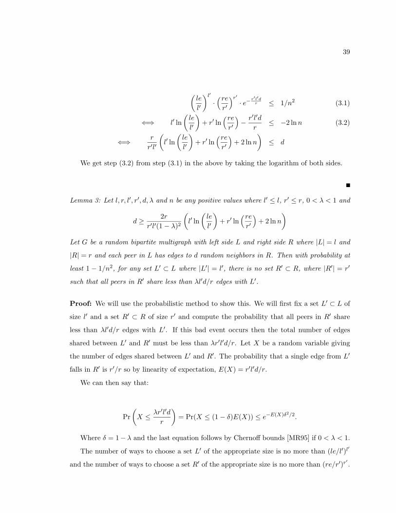
39
(le
l′
)l′
·(re
r′
)r′
· e− r′l′dr ≤ 1/n2 (3.1)
⇐⇒ l′ ln(
le
l′
)+ r′ ln
(re
r′
)− r′l′d
r≤ −2 lnn (3.2)
⇐⇒ r
r′l′
(l′ ln
(le
l′
)+ r′ ln
(re
r′
)+ 2 lnn
)≤ d
We get step (3.2) from step (3.1) in the above by taking the logarithm of both sides.
Lemma 3: Let l, r, l′, r′, d, λ and n be any positive values where l′ ≤ l, r′ ≤ r, 0 < λ < 1 and
d ≥ 2r
r′l′(1 − λ)2
(l′ ln
(le
l′
)+ r′ ln
(re
r′
)+ 2 lnn
)Let G be a random bipartite multigraph with left side L and right side R where |L| = l and
|R| = r and each peer in L has edges to d random neighbors in R. Then with probability at
least 1 − 1/n2, for any set L′ ⊂ L where |L′| = l′, there is no set R′ ⊂ R, where |R′| = r′
such that all peers in R′ share less than λl′d/r edges with L′.
Proof: We will use the probabilistic method to show this. We will first fix a set L′ ⊂ L of
size l′ and a set R′ ⊂ R of size r′ and compute the probability that all peers in R′ share
less than λl′d/r edges with L′. If this bad event occurs then the total number of edges
shared between L′ and R′ must be less than λr′l′d/r. Let X be a random variable giving
the number of edges shared between L′ and R′. The probability that a single edge from L′
falls in R′ is r′/r so by linearity of expectation, E(X) = r′l′d/r.
We can then say that:
Pr(
X ≤ λr′l′d
r
)= Pr(X ≤ (1 − δ)E(X)) ≤ e−E(X)δ2/2.
Where δ = 1− λ and the last equation follows by Chernoff bounds [MR95] if 0 < λ < 1.
The number of ways to choose a set L′ of the appropriate size is no more than (le/l′)l′
and the number of ways to choose a set R′ of the appropriate size is no more than (re/r′)r′ .

40
So the probability that no two subsets L′ of size l′ and R′ of size r′ have this bad event
occur is
(le
l′
)l′
·(re
r′
)r′
· e− r′l′dδ2
2r .
Below we solve for appropriate d such that this probability is less than 1/n2.
(le
l′
)l′
·(re
r′
)r′
· e− r′l′dδ2
2r ≤ 1/n2 (3.3)
⇐⇒ l′ ln(
le
l′
)+ r′ ln
(re
r′
)− r′l′dδ2
2r≤ −2 lnn (3.4)
⇐⇒ 2r
r′l′(1 − λ)2
(l′ ln
(le
l′
)+ r′ ln
(re
r′
)+ 2 lnn
)≤ d
We get step (3.4) from step (3.3) in the above by taking the logarithm of both sides.
Lemma 4: Let l, r, r′, d, β′ and n be any positive values where l′ ≤ l, β′ > 1 and
d ≥ 4r
r′l(β′ − 1)2(r′ ln
(re
r′
)+ 2 lnn
)Let G be a random bipartite multigraph with left side L and right side R where |L| = l and
|R| = r and each peer in L has edges to d random neighbors in R. Then with probability at
least 1 − 1/n2, there is no set R′ ⊂ R, where |R′| = r′ such that all peers in R′ have degree
greater than β′ld/r.
Proof: We will again use the probabilistic method to show this. We will first fix a set
R′ ⊂ R of size r′ and compute the probability that all peers in R′ have degree greater than
β′ld/r. If this bad event occurs then the total number of edges shared between L and R′
must be at least β′r′ld/r. Let X be a random variable giving the number of edges shared
between L and R′. The probability that a single edge from L falls in R′ is r′/r so by linearity
of expectation, E(X) = r′ld/r.
We can then say that:
41
Pr(
X ≥ β′r′ld
r
)= Pr(X ≥ (1 + δ)E(X)) ≤ e−E(X)δ2/4.
Where δ = β′ − 1 and the last equation follows by Chernoff bounds [MR95] if 1 < β′ <
2e − 1.
The number of ways to choose a set R′ of the appropriate size is no more than (re/r′)r′ .
So the probability that no subset R′ of size r′ has this bad event occur is
(re
r′
)r′
· e− r′l′dδ2
4r .
Below we solve for appropriate d such that this probability is less than 1/n2.
(re
r′
)r′
· e− r′ldδ2
4r ≤ 1/n2 (3.5)
⇐⇒ r′ ln(re
r′
)− r′ldδ2
4r≤ −2 lnn (3.6)
⇐⇒ 4r
r′l(β′ − 1)2(r′ ln
(re
r′
)+ 2 ln n
)≤ d
We get step (3.6) from step (3.5) in the above by taking the logarithm of both sides.
42
Chapter 4
THE DYNAMICALLY ATTACK-RESISTANT NETWORK
In this chapter, we describe our Dynamically Attack-Resistant Network. Section 4.1
describes the new “Dynamic Attack Resistant” property, Section 4.2 describes our network,
and Section 4.3 gives the proofs that our network is dynamically attack-resistant and has
good performance.
4.1 Dynamic Attack Resistance
To better address attack-resistance in peer-to-peer networks which are faced with massive
peer turnover, we define a new notion of attack-resistance: dynamic attack-resistance. First,
we assume an adversarial fail-stop model – at any time, the adversary has complete visibility
of the entire state of the system and can choose to ”delete” any peer it wishes. A ”deleted”
peer stops functioning immediately, but is not assumed to be Byzantine. Second, we require
our network to remain “robust” at all times provided that in any time interval during which
the adversary deletes some number of peers, some larger number of new peers join the
network. The network remains “robust” in the sense that an arbitrarily large fraction of
the live peers can access an arbitrarily large fraction of the content.
More formally, we say that an adversary is limited if for some constants γ > 0 and δ > γ,
during any period of time in which the adversary deletes γn peers from the network, at least
δn new peers join the network (where n is the number of peers initially in the network).
Each new peer that is inserted knows only one other random peer currently in the network.
For such a limited adversary, we seek to maintain a robust network for indexing up to n
data items. Although the number of indexed data items remains fixed, the number of peers
in the network will fluctuate as nodes are inserted and deleted by the adversary.
We say that a content addressable network (CAN) is ε-robust at some particular time
if all but an ε fraction of the peers in the CAN can access all but an ε fraction of the data

43
items.
Finally, we say that a CAN (initially containing n peers) is ε-dynamically attack-resistant,
if, with high probability, the CAN is always ε-robust during a period when a limited adver-
sary deletes a number of peers polynomial in n.
In section 4.2, we present an ε-dynamically attack-resistant CAN for any arbitrary ε > 0,
and any constants γ and δ such that γ < 1 and δ > γ + ε. Our CAN stores n data items1,
and has the following characteristics:
1. With high probability, at any time, an arbitrarily large fraction of the nodes can find
an arbitrarily large fraction of the data items.
2. Search takes time O(log n) and requires O(log3 n) messages in total.
3. Every peer maintains pointers to O(log3 n) other peers.
4. Every peer stores O(log n) data items.
5. Peer insertion takes time O(log n).
The constants in these resource bounds are functions of ε, γ and δ. The technical
statement of this result is presented in Theorem 20.
We note that, as we have defined it, an ε-dynamically attack-resistant CAN is ε-robust
for only a polynomial number of peer deletions by the limited adversary. To address this
issue, we imagine that very infrequently, there is an all-to-all broadcast among all live
peers to reconstruct the CAN(details of how to do this are in [FS02]). Even with these
infrequent reconstructions, the amortized cost per insertion will be small. Our main theorem
is provided below.
Theorem 20 Let n be fixed. Then for all ε > 0 and value P which is polynomial in n,
there exist constants k1(ε), k2(ε) and k3(ε) and k4(ε) such that the following holds with high
probability for the CAN for deletion of up to P peers by the limited adversary:
1For simplicity, we’ve assumed that the number of items and the number of initial nodes is equal. However,for any n nodes and m ≥ n data items, our scheme will work, where the search time remains O(log n),the number of messages remains O(log3 n), and the storage requirements are O(log3 n × m/n) per node.
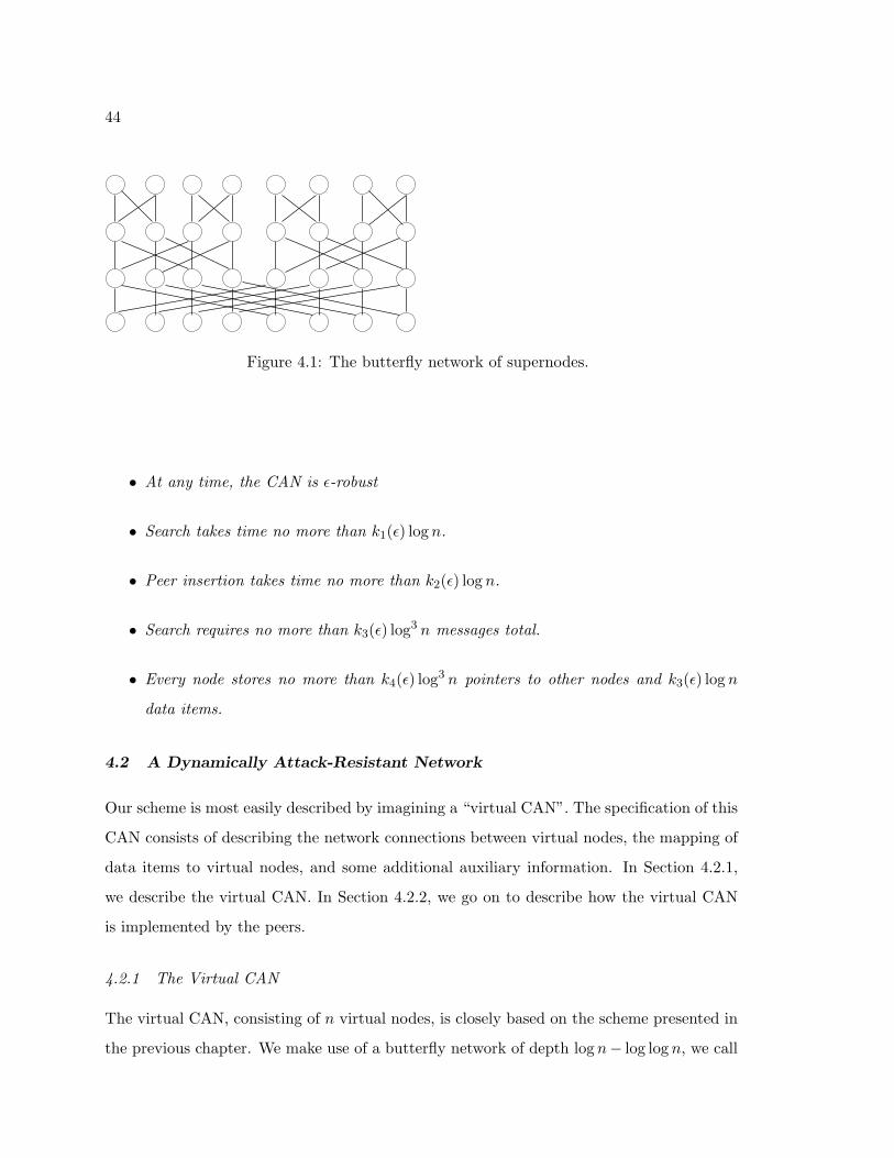
44
Figure 4.1: The butterfly network of supernodes.
• At any time, the CAN is ε-robust
• Search takes time no more than k1(ε) log n.
• Peer insertion takes time no more than k2(ε) log n.
• Search requires no more than k3(ε) log3 n messages total.
• Every node stores no more than k4(ε) log3 n pointers to other nodes and k3(ε) log n
data items.
4.2 A Dynamically Attack-Resistant Network
Our scheme is most easily described by imagining a “virtual CAN”. The specification of this
CAN consists of describing the network connections between virtual nodes, the mapping of
data items to virtual nodes, and some additional auxiliary information. In Section 4.2.1,
we describe the virtual CAN. In Section 4.2.2, we go on to describe how the virtual CAN
is implemented by the peers.
4.2.1 The Virtual CAN
The virtual CAN, consisting of n virtual nodes, is closely based on the scheme presented in
the previous chapter. We make use of a butterfly network of depth log n− log log n, we call

45
the nodes of the butterfly network supernodes (see Figure 1). Every supernode is associated
with a set of virtual nodes. We call a supernode at the topmost level of the butterfly a
top supernode, one at the bottommost level of the network a bottom supernode and one at
neither the topmost or bottommost level a middle supernode.
We use a set of hash functions for mapping virtual nodes to supernodes of the butterfly
and for mapping data items to supernodes of the butterfly. We assume these hash functions
are approximately random. 2
The virtual network is constructed as follows:
• We choose an error parameter ε > 0, and as a function of ε we determine constants
C, D, α and β. (This is done in the same way specified in the last chapter).
• Every virtual node v is hashed to C random top supernodes (we denote by T (v) the
set of C top supernodes v hashes to), C random bottom supernodes (denoted B(v))
and C log n random middle supernodes (denoted M(v)) to which the virtual node will
belong.
• All the virtual nodes associated with any given supernode are connected in a clique.
(We do this only if the set of virtual nodes in the supernode is of size at least αC lnn
and no more than βC ln n.)
• Between two sets of virtual nodes associated with two supernodes connected in the
butterfly network, we have a complete bipartite graph. (We do this only if both sets
of virtual nodes are of size at least αC lnn and no more than βC lnn.)
• We map the n data items to the n/ log n bottom supernodes in the butterfly: each
data item, say d, is hashed to D random bottom supernodes; we denote by S(d) the
set of bottom supernodes that data item d is mapped to. (Typically, we would not
hash the entire data item but only it’s title, e.g., “Singing in the Rain”).
2We use the random oracle model ([BR93]) for these hash function, it would have sufficed to have aweaker assumption such as that the hash functions are expansive.

46
• The data item d is then stored in all the component virtual nodes of S(d) (if any
bottom supernode has more than βB ln n data items hashed to it, it drops out of the
network.)
• Finally, we map the meta-data associated with each of the n virtual nodes in the
network to the n/ log n bottom supernodes in the butterfly. For each virtual node
v, information about v is mapped to D bottom supernodes. We denote by I(v) the
set of bottom supernodes storing information about virtual node v. (if any bottom
supernode has more than βB lnn virtual nodes hashed to it, it drops out of the
network.)
• For each virtual node v in the network, we do the following:
1. We store the id of v on all component virtual nodes of I(v).
2. A complete bipartite graph is maintained between the virtual nodes associated
with supernodes I(v) and the virtual nodes in supernodes T (v), M(v) and B(v).
4.2.2 Implementation of Virtual CAN by Peers
Each peer that is currently live will map to exactly one node in the virtual network and
each node in the virtual network will be associated with at most one live peer. At all times
we will maintain the following two invariants:
1. If peers p1 and p2 map to virtual nodes x and y and x links to y in the virtual network,
then p1 links to p2 in the physical overlay network.
2. If peer p maps to virtual node x, then p stores the same data items that x stores in
the virtual network.
Recall that each virtual node in the network participates in C top, C log n middle and
C bottom supernodes. When a virtual node v participates in a supernode s in this way,
we say that v is a member of s. For a supernode s, we define V (s) to be the set of virtual

47
nodes which are members of s. Further we define P (s) to be the set of live peers which map
to virtual nodes in V (s).
4.2.3 Search for a Data Item
We will now describe the protocol for searching for a data item from some peer p in the
network. We will let v be the virtual node p maps to and let d be the desired data item.
1. Let b1, b2, . . . , bD be the bottom supernodes in the set S(d).
2. Let t1, t2, . . . , tC be the top supernodes in the set T (v).
3. Repeat in parallel for all values of k between 1 and C:
(a) Let = 1.
(b) Repeat until successful or until > B:
i. Let s1, s2, . . . sm be the supernodes in the path in the butterfly network from
tk to the bottom supernode b.
• Transmit the query to all peers in the set P (s1).
• For all values of j from 2 to m do:
– The peers in P (sj−1) transmit the query to all the peers in P (sj).
• When peers in the bottom supernode are reached, fetch the content from
whatever peer has been reached.
• The content, if found, is transmitted back along the same path as the
query was transmitted downwards.
ii. Increment .
4.2.4 Content and Peer Insertion
An algorithm for inserting new content into the network is presented in the previous chapter.
In this section, we describe the new algorithm for peer insertion. We assume that the new
peer knows one other random live peer in the network. We call the new peer p and the
random, known peer p′.

48
1. p first chooses a random bottom supernode, which we will call b. p then searches
for b in the manner specified in the previous section. The search starts from the top
supernodes in T (p′) and ends when we reach the node b(or fail).
2. If b is successfully found, we let W be the set of all virtual nodes, v , such that meta-
data for v is stored on the peers in P (b). We let W ′ be the set of all virtual nodes in
W which are not currently mapped to some live peer.
3. If b can not be found, or if W ′ is empty, p does not map to any virtual node. Instead
it just performs any desired searches for data items from the top supernodes, T (p′).
4. If there is some virtual node v in W ′, p takes over the role of v as follows:
(a) Let S = T (v)∪M(v)∪B(v). Let F be the set of all supernodes, s in S such that
P (s) is not empty. Let E = S − F .
(b) For each supernode s in F :
i. Let R be the set of supernodes that neighbor s in the butterfly.
ii. p copies the links to all peers in P (r) for each supernode r in R. These links
can all be copied at once from one of the peers in P (s). Note that each peer
in P (b) contains a pointer to some peer in P (s).
iii. p notifies all peers to which it will be linking to also link to it. For each
supernode r in R, p sends a message to one peer in P (r) notifying it of p’s
arrival. The peer receiving the message then relays the message to all peers
in P (r). These peers then all point to p.
iv. If s is a bottom supernode, p copies all the data items that map to s. It
copies these data items from some peer in P (s).
(c) If E is non-empty, we will do one broadcast to all peers that are reachable from
p. We will first broadcast from the peers in all top supernodes in T (p) to the
peers in all reachable bottom supernodes. We will then broadcast from the peers

49
in these bottom supernodes back up the butterfly network to the peers in all
reachable top supernodes: 3
i. p broadcasts the id of v along with the ids of all the supernodes in E. All
peers that receive this message, which are in supernodes neighboring some
supernode in E will connect to p.
ii. In addition to forging these links, we seek to retrieve data items for each
bottom supernode which is in the set E. Hence, we also broadcast the ids
for these data items. We can retrieve these data items if they are still stored
on other peers.4
4.3 Proofs
In this section, we provide the proof of Theorem 20 and proofs of the claimed performance
properties for the network given in the last section.
4.3.1 Dynamic Attack-Resistance
We will be using the following two lemmas which follow from results in the previous chapter.
We first define a peer as ε-good if it is connected to all but 1− ε of the bottom supernodes.
Lemma 21 Assume at any time, at least κn of the virtual nodes map to live peers for some
κ < 1. Then for any ε, we can choose appropriate constants C and D for the virtual network
such that at all times, all but an ε fraction of the top supernodes are connected to all but an
ε fraction of the bottom nodes.
Proof: This lemma follows directly from Theorem 1 in the last chapter by plugging in
appropriate values.
3This broadcast takes O(log n) time but requires a large number of messages. However, we anticipatethat this type of broadcast will occur infrequently. In particular, under the assumption of random failures,this broadcast will never occur with high probability.
4We note that, using the scheme in [AKK+00], we can retrieve the desired data items, even in the casewhere we are connected to no more than n/2 live peers. To use this scheme, we need to store, for eachdata item of size s, some extra data of size O(s/n) on each node in the network. Details on how to dothis are ommitted.

50
Lemma 22 Assume at any time, at least κn of the virtual nodes map to live peers for
some κ < 1. Then for any ε < 1/2, we can choose appropriate constants C and D for the
virtual network such that at all times, all ε-good nodes are connected in one component with
diameter O(log n).
Proof: By Lemma 21, we can choose C and D such that all ε-good peers can reach more
than a 1/2 fraction of the bottom supernodes. Then for any two ε-good peers, there must
be some bottom supernode such that both peers are connected to that same supernode.
Hence, any two ε-good peers must be connected. In addition, the path between these two
ε-good peers must be of length O(log n) since the path to any bottom supernode is of length
O(log n)
We now give the proof of Theorem 20 which is restated here.
Theorem 20: For all ε > 0 and value P which is polynomial in n, there exist constants k1(ε),
k2(ε) and k3(ε) and k4(ε) such that the following holds with high probability for the CAN
for deletion of up to P peers by the limited adversary:
• At any time, the CAN is ε-robust
• Search takes time no more than k1(ε) log n.
• Peer insertion takes time no more than k2(ε) log n.
• Search requires no more than k3(ε) log3 n messages total.
• Every node stores no more than k4(ε) log3 n pointers to other nodes and k3(ε) log n
data items.
Proof: We briefly sketch the argument that our CAN is dynamically attack-resistant. The
proofs for the time and space bounds are given in the next two subsections.

51
For concreteness, we will prove dynamic attack-resistance with the assumption that
2n/10 peers are added whenever (1/10 − ε)n peers are deleted by the adversary. The
argument for the general case is similar. Consider the state of the system when exactly
2n/10 virtual nodes map to no live peers. We will focus on what happens for the time
period during which the adversary kills off (1/10 − ε)n more peers. By assumption, during
this time, 2n/10 new peers join the network. In this proof sketch, we will show that with
high probability, the number of virtual nodes which are not live at the end of this period is
no more than 2n/10. The general theorem follows directly.
We know that Lemma 21 applies during the time period under consideration since there
are always at least n/2 live virtual nodes. Let R be the set of virtual nodes that at some
point during this time period are not ε-good. By Lemma 22, peers in virtual nodes that are
not in the set R have been connected in the large component of ε-good nodes throughout the
considered time interval. Thus these peers have received information broadcasted during
successful peer insertions. However, the peers mapping to virtual nodes in R may at some
point have not been connected to all the other ε-good nodes and so may not have have
received information broadcasted by inserted peers. We note that |R| is no more than εn
by Lemma 21 (since even with no insertions in the network, no more than εn virtual nodes
would be not be ε-good at any point in the time period under consideration). Hence we
will just assume that those peers with stale information, i.e. the peers in R, are dead. To
do this, we will assume that the number of adversarial node deletions is n/10. (We further
note that all peers which are not ε-good will actually be considered dead by all peers which
are ε-good. This is true since no bottom supernode reachable from an ε-good node will have
a link to a peer which is not ε-good. Hence, such a virtual node will be fair game for a new
peer to map to.)
We claim that during the time interval, at least n/10 of the inserted peers will map to
virtual nodes. Assume not. Then there is some subset, S, of the 2n/10 peers that were
inserted such that |S| = n/10 and all peers in S did not reach any bottom supernodes with
information on virtual nodes that had no live peers. Let S′ be the set of peers in S that
both 1) had an initial connection to an ε-good peer and 2) reached the bottom supernode
which they searched for after connecting. We note that with high probability, |S′| = θ(n)
52
since each new peer connects to a random peer (of which most are ε-good) and since most
bottom supernodes are reachable from an ε-good peer.
Now let B′ be the set of bottom supernodes that are visited by peers in S′. With high
probability |B′| = θ(n/ log n). Finally let V ′ be the set of virtual nodes that supernodes in
B′ have information on. For D (the constant defined in the virtual network section) chosen
sufficiently large, |V ′| must be greater than 9n/10 (by expansion properties between the
bottom supernodes and the virtual nodes they have information on). But by assumption,
there must be some subset V of virtual node ids which are empty after the insertions where
|V | ≥ n/10. But this is a contradiction since we know that the set of virtual nodes that the
new peers in S′ tried to map to was of size greater than 9n/10
Hence during the time that n/10 peers were deleted from the network, at least n/10
virtual nodes were newly mapped to live peers. This implies that the number of virtual
peers not mapped to live nodes can only have decreased. Thus the number of virtual
peers not mapped to live nodes will not increase above 2n/10 after any interval with high
probability.
Time
That the algorithm for searching for data items takes O(log n) time and O(log2 n) messages
is proven in the last chapter.
The common and fast case for peer insertion is when all supernodes to which the new
peer’s virtual node belongs already have some peer in them. In this case, we spend constant
time processing each one of these supernodes so the total time spent is O(log n).
In the degenerate case where there are supernodes which have no live nodes in them,
a broadcast to all nodes in the network is required. Insertion time will still be O(log n)
since the connected component of ε-good nodes has diameter O(log n). However we will
need to send O(n) messages for the insertion. Unfortunately, the adversary can force this
degenerate case to occur for a small (less than ε) fraction of the node insertions. However
if the node deletions are random instead of adversarial, this case will never occur in the
53
interval in which some polynomial number of nodes are deleted.
Space
Each node participates in C top supernodes. The number of links that need to be stored
to play a role in a particular top supernode is O(log n). This includes links to other nodes
in the supernode and links to the nodes that point to the given top supernode.
Each node participates in C log n middle supernodes. To play a role in a particular
middle supernode takes O(log n) links to point to all the other nodes in the supernode and
O(log n) links to point to nodes in all the neighboring supernodes. In addition, each middle
supernode has O(log n) roles associated with it and each of these roles is stored in D bottom
supernodes. Hence each node in the supernode needs O(log2n) links back to all the nodes
in the bottom supernodes which store roles associated with this middle supernode.
Each node participates in C bottom supernodes. To play a role in a bottom supernode
requires storing O(log n) data items. It also requires storing O(log n) links to other nodes in
the supernode along with nodes in neighboring supernodes. In addition, it requires storing
O(log n) links for each of the O(log n) supernodes for each of the O(log n) roles that are
stored at the node. Hence the total number of links required is O(log3 n).
4.4 Conclusion
In these last three chapters, we have defined a new notion of fault-tolerance called attack-
resistance and have given three types of peer-to-peer networks which are attack-resistant.
We call a network attack-resistant if it’s the case that after an adversary deletes or controls
an arbitrarily large fraction of the peers in the network, an arbitrarily large fraction of the
remaining peers can still access an arbitrarily large fraction of the content in the network.
We emphasize that faults in the network are not assumed to be simply independent but
rather the result of an orchestrated attack by an omniscient adversary.
We have presented three networks that have attack-resistant properties. The Deletion
Resistant Network is resistant to an adversary which can delete peers from the network. The
Control Resistant Network is resistant to an adversary which can cause arbitrary Byzantine

54
faults. This network is strictly more robust than the Deletion Resistant Network in the
sense that the adversary can either kill the peers it controls or make them send arbitrary
messages. Finally, the Dynamically Attack-Resistant Network is robust even in the presence
of repeated, massive adversarial attacks. This network is robust only in the presence of
adversarial deletion and it depends on the fact that enough new peers are added to the
network to replace the peers that are deleted.
To the best of our knowledge, these three networks are the first that have been proposed
which are both scalable and attack-resistant. We note that while these networks have good
asymptotic resource bounds, the constants in the asymptotics are still too large to make
the networks practical. Reducing these constants is an area for future work.

55
Chapter 5
INTRODUCTION TO DATA MIGRATION
In this chapter, we describe our work on the problem of data migration. Section 5.1
gives an overview of the real-world data migration problem, Section 5.2 gives the variants
of this problem for which we will present algorithms, Section 5.3 gives the theoretical and
empirical results for our algorithms for these variants and Section 5.4 gives related work.
5.1 High Level Description of the Data Migration Problem
The input to the migration problem is an initial and final configuration of data objects on
devices, and a description of the storage system (the storage capacity of each device, the
underlying network connecting the devices, etc.) Our goal is to find a migration plan that
uses the existing network connections between storage devices to move the data from the
initial configuration to the final configuration in the minimum amount of time. For obvious
reasons, we require that all intermediate configurations in the plan be valid: they must
obey the capacity constraints of the storage devices as well as usability requirements of the
online system. The motivation for these requirements is that the migration process can be
stopped at any time and the online system should still be able to run and maintain full
functionality.
The time it takes to perform a migration is a function of the sizes of the objects being
transferred, the network link speeds and the degree of parallelism in the plan. A crucial
constraint on the legal parallelism in any plan is that each storage device can be involved
in the transfer (either sending or receiving, but not both) of only one object at a time.
Most variants one can imagine on this problem are NP-complete. The migration problem
for networks of arbitrary topology is NP-complete even if all objects are the same size and
each device has only one object that must be moved off of it. The problem is also NP-
complete when there are just two storage devices connected by a link, if the objects are of

56
arbitrary sizes.1
We will always make the following two assumptions:
• the data objects are all the same size;
• there is at least one free space on each storage device in both the initial and final
configurations of the data.
The first assumption is quite reasonable in practice if we allow ourselves to subdivide
the existing variable sized objects into unit sized pieces, since the time it takes to send the
subdivided object is about the same as the time it takes to send the entire object. The
second assumption is also reasonable in practice, since free space somewhere is required in
order to move any objects, and having only one free space in the entire network would limit
the solution to being sequential. We note that this second assumption allows us to think of
time in discrete intervals or time steps.
5.2 Data Migration Variants
5.2.1 Identical Devices Connected in Complete Networks
In Chapters 6 and 7, we focus on the following challenging special case of the migration
problem. In addition to our two standard assumptions (fixed object size and one extra free
space), in these two Chapters we will make the following two additional assumptions
• there is a direct bidirectional link between each pair of devices and each link has the
same bandwidth.
• every device has the same read and write speed
Both of these assumptions are reasonable if we assume that the storage devices are
connected in a local area network (LAN), (for example in a disk farm). The first assumption
is reasonable since the topologies in LANs are generally very close to being complete. The
1This observation was made by Dushyanth Narayanan.

57
v4
v3v2
v1 v4
v3v2
v1
Initial: Demand Graph:Goal:
a
b,c d
b,c
a
dv4
v3v2
v1
c b da
Figure 5.1: An example demand graph. v1,v2,v3,v4 are devices in the network and theedges in the first two graphs represent links between devices. a,b,c,d are the data objectswhich must be moved from the initial configuration to the goal configuration.
second assumption is reasonable since an organization building a LAN of storage devices
might tend to buy devices which have equal performance characteristics. For wide area
networks, these assumptions are much less reasonable. In Chapter 8, we will show how to
generalize these results to arbitrary topologies and heterogeneous device speeds.
With these assumptions, we are led to describe the input to our problem as a directed
multigraph G = (V, E) without self-loops that we call the demand graph. Each vertex in the
demand graph corresponds to a storage device, and each directed edge (u, v) ∈ E represents
an object that must be moved from storage device u (in the initial configuration) to storage
device v (in the final configuration). An example of how a demand graph is defined based
on an initial and goal configuration is given in Figure 5.1
Since we are considering fixed-size objects, and each device can be involved in only one
send or receive at a time, our migration plan can be divided into stages where each stage
consists of a number of compatible sends, i.e., each stage is a matching. Thus, we can observe
that the special case of our problem when there are no capacity constraints on the storage
devices, and there are no unused devices, is precisely the multigraph edge coloring problem
(the directionality of the edges becomes irrelevant and the colors of the edges represent the

58
time steps when objects are sent). This problem is of course NP-complete, but there are
very good approximation algorithms for it, as we shall review in Section 5.4. The storage
migration application introduces two very interesting twists on the traditional edge coloring
problem: edge coloring with bypass nodes and edge coloring with space constraints. We
describe these variants in the next two sections.
Bypass Nodes
In the first variant on edge coloring, we consider the question of whether indirect plans can
help us to reduce the time it takes to perform a migration. In an indirect plan, an object
might temporarily be sent to a storage device other than its final destination. Figure 5.2
gives an example of how this can significantly reduce the number of stages in the migration
plan. As a first step towards attacking the problem of constructing near-optimal indirect
plans, we introduce the concept of a bypass node. A bypass node is an extra storage device
that can be used to store objects temporarily in an indirect plan. (In practice, some of the
storage devices in the system will either not be involved or will be only minimally involved
in the migration of objects and these devices can be used as bypass nodes.) A natural
question to then ask is: what is the tradeoff between the number of bypass nodes available
and the time it takes to perform the migration? In particular, how many bypass nodes
are needed in order to perform the migration in ∆(G) steps, where ∆(G) (or ∆ where G
is understood) is the maximum total degree of any node in the demand graph G. (∆ is a
trivial lower bound on the number of steps needed, no matter how many bypass nodes are
available.)
An optimal direct migration takes at least χ′ parallel steps where χ′ is the chromatic
index of the demand graph (the minimum number of colors in any edge coloring). If our
solution is not required to send objects directly from source to destination it is possible
that there is a migration plan that takes less than χ′ stages. In general, our goal will be
to use a small number of bypass nodes, extra storage devices in the network available for
temporarily storing objects, to perform the migration in essentially ∆ stages.
Definition 23 A directed edge (v, w) in a demand graph is bypassed if it is replaced by two
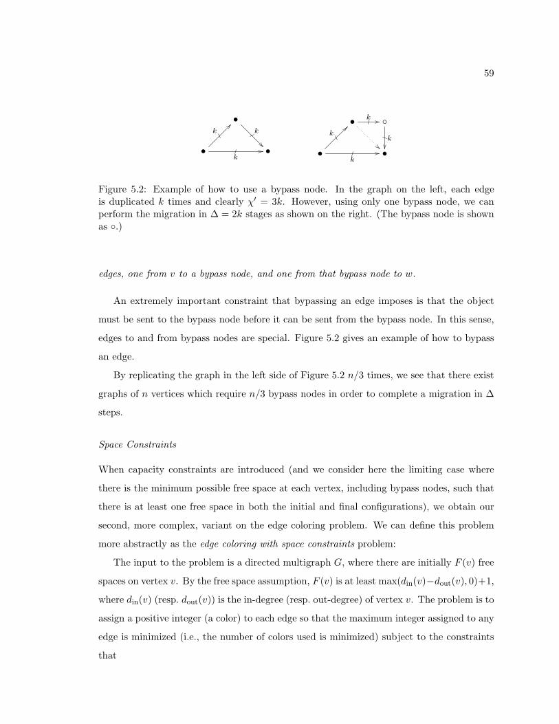
59
•k
•
k
k•
• k k
•
k
k•
Figure 5.2: Example of how to use a bypass node. In the graph on the left, each edgeis duplicated k times and clearly χ′ = 3k. However, using only one bypass node, we canperform the migration in ∆ = 2k stages as shown on the right. (The bypass node is shownas .)
edges, one from v to a bypass node, and one from that bypass node to w.
An extremely important constraint that bypassing an edge imposes is that the object
must be sent to the bypass node before it can be sent from the bypass node. In this sense,
edges to and from bypass nodes are special. Figure 5.2 gives an example of how to bypass
an edge.
By replicating the graph in the left side of Figure 5.2 n/3 times, we see that there exist
graphs of n vertices which require n/3 bypass nodes in order to complete a migration in ∆
steps.
Space Constraints
When capacity constraints are introduced (and we consider here the limiting case where
there is the minimum possible free space at each vertex, including bypass nodes, such that
there is at least one free space in both the initial and final configurations), we obtain our
second, more complex, variant on the edge coloring problem. We can define this problem
more abstractly as the edge coloring with space constraints problem:
The input to the problem is a directed multigraph G, where there are initially F (v) free
spaces on vertex v. By the free space assumption, F (v) is at least max(din(v)−dout(v), 0)+1,
where din(v) (resp. dout(v)) is the in-degree (resp. out-degree) of vertex v. The problem is to
assign a positive integer (a color) to each edge so that the maximum integer assigned to any
edge is minimized (i.e., the number of colors used is minimized) subject to the constraints
that
60
• no two edges incident on the same vertex have the same color, and
• for each i and each vertex v, c(i)in (v) − c
(i)out(v) ≤ F (v), where c
(i)in (v) (resp. c
(i)out(v)) is
the number of in-edges (resp. out-edges) incident to v with color at most i.
The second condition, which we refer to as the space constraint condition, captures the
requirement that at all times the space consumed by data items moved onto a storage device
minus the space consumed by data items moved off of that storage device can not exceed
the initial free space on that device.
Obviously, not all edge-colorings of a multigraph (with edge directionality ignored) will
satisfy the conditions of an edge-coloring with space constraints. However, it remains unclear
how much harder this problem is than standard edge coloring.
5.2.2 Heterogeneous Device Speeds and Edge Capacities
In data migration projects over wide area networks, the assumption that topology is com-
plete and that the storage devices all have the same disk speeds become much less reason-
able. Thus the final variant of the data migration problem we consider (in Chapter 8) is
the case where the storage devices have different speeds and the network links have variable
bandwidths.
5.3 Our Results
5.3.1 Algorithmic Results on Identical Devices and Complete Topologies
Table 5.1 gives a summary of the theoretical results for all algorithms presented in this thesis
for the problem of data migration on identical devices and complete topologies. Below we
summarize the results for the algorithms in this table with the best theoretical bounds. The
results are given for a graph with n vertices and maximum degree ∆. (These algorithms
are described in Chapter 6):
• 2-factoring : an algorithm for edge coloring that uses at most n/3 bypass nodes and
at most 2 ∆/2 colors.
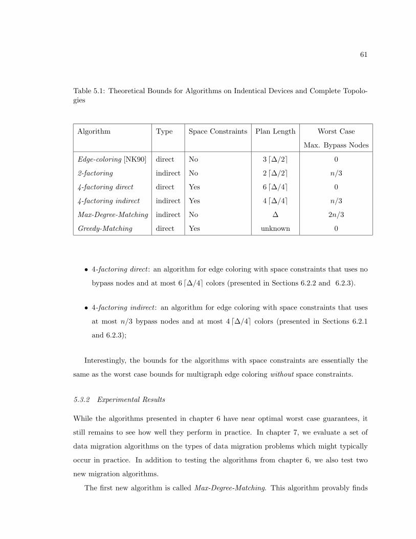
61
Table 5.1: Theoretical Bounds for Algorithms on Indentical Devices and Complete Topolo-gies
Algorithm Type Space Constraints Plan Length Worst Case
Max. Bypass Nodes
Edge-coloring [NK90] direct No 3 ∆/2 0
2-factoring indirect No 2 ∆/2 n/3
4-factoring direct direct Yes 6 ∆/4 0
4-factoring indirect indirect Yes 4 ∆/4 n/3
Max-Degree-Matching indirect No ∆ 2n/3
Greedy-Matching direct Yes unknown 0
• 4-factoring direct : an algorithm for edge coloring with space constraints that uses no
bypass nodes and at most 6 ∆/4 colors (presented in Sections 6.2.2 and 6.2.3).
• 4-factoring indirect : an algorithm for edge coloring with space constraints that uses
at most n/3 bypass nodes and at most 4 ∆/4 colors (presented in Sections 6.2.1
and 6.2.3);
Interestingly, the bounds for the algorithms with space constraints are essentially the
same as the worst case bounds for multigraph edge coloring without space constraints.
5.3.2 Experimental Results
While the algorithms presented in chapter 6 have near optimal worst case guarantees, it
still remains to see how well they perform in practice. In chapter 7, we evaluate a set of
data migration algorithms on the types of data migration problems which might typically
occur in practice. In addition to testing the algorithms from chapter 6, we also test two
new migration algorithms.
The first new algorithm is called Max-Degree-Matching. This algorithm provably finds
62
a migration taking ∆ steps while using no more than 2n/3 bypass nodes. We empirically
compare this to 2-factoring. While 2-factoring has better theoretical bounds than Max-
Degree-Matching, we will see that Max-Degree-Matching uses fewer bypass nodes on almost
all tested demand graphs.
For migration with space constraints, we introduce a new algorithm, Greedy-Matching,
which uses no bypass nodes. We know of no good bound on the number of time steps taken
by Greedy-Matching in the worst case; however, in our experiments, Greedy-Matching often
returned plans with very close to ∆ time steps and never took more than 3∆/2 time steps.
This compares favorably with 4-factoring direct, which also never uses bypass nodes but
which always takes essentially 3∆/2 time steps.
Even though these new algorithms have inferior worst case guarantees, we find that, in
practice, they usually outperform the algorithms having better theoretical guarantees. In
addition, we find that for all the algorithms, the theoretical guarantees on performance are
much worse than what actually occurs in practice. For example, even though the worst case
for the number of bypass nodes needed by many of the algorithms is n/3, in our experiments,
we almost never required more than about n/30 bypass nodes.
5.3.3 Algorithmic Results for Heterogeneous Device Speeds and Link Capacities
While the assumptions of equivalent device speeds and complete topologies are likely to
hold for a devices that are connected in a local area network, these assumptions are not
reasonable for storage devices connected in a wide area network. Thus, in Chapter 8, we
consider migration in the more difficult case where the storage devices can have different
read and write speeds and where the capacities of edges between any pair of devices can be
arbitrary.
In Chapter 8, we will consider three special cases of this general problem:
• Edge-Coloring with Speeds: We assume still that there is a bidirectional link between
each pair of devices and all links have the same bandwidth. However, the devices now
can have varying speeds.

63
• Migration on Trees: Here we assume that the network connecting the storage devices
is a tree. The storage devices can have varying speeds and the link bandwidths can
be variable.
• Migration with Splitting : Here we consider both variable link bandwidths and variable
device speeds. However we make the assumption that we can split the data objects
into a certain number of pieces.
For these problems, we present the following results:
• Edge-Coloring with Speeds: We give an algorithm which always finds a migration plan
with length within a factor of 3/2 of the optimal length.
• Migration on Trees: We give an algorithm which always finds a migration plan with
length within a factor of 3/2 of the optimal length.
• Migration with Splitting : We give an algorithm which can find a migration plan with
length within a factor of (1 + ε) of optimal for any ε > 0 provided that the data
objects can be split into a certain number of pieces (the number of pieces required is
a function of ε and the length of the optimal plan).
5.4 Related Work
5.4.1 Identical Devices Connected in Complete Networks
There is much related work for the data migration problem where G is a complete graph,
all objects are the same size and all nodes have speed 1 the basic migration problem. As
noted previously, this basic problem is the well-known edge coloring problem. There are
several other problems which are equivalent to edge coloring including h-relations [GHKS98,
SSO00], file transfer [ECL85], and biprocessor task scheduling on dedicated processors
[Kub96].
There are at least three decades of work on the edge-coloring problem. The minimum
number of colors needed to edge-color a graph G is called the chromatic index of G (χ′(G)).
64
For a given graph G, computing χ′(G) exactly is of course NP-Hard [NK90]. For simple
graphs (i.e. graphs with no multiple edges) Vizing [Viz64] gives a polynomial time (∆ + 1)-
approximation algorithm. For multigraphs, the current best approximation algorithm given
by Nishizeki and Kashigawa [NK90] uses no more than 1.1χ′(G) + .8 colors. As stated
previously, the maximum degree of the graph ∆(G) is a trivial lower bound on χ′(G).
Sanders and Solis-Oba [SSO00] study the problem of edge-coloring with indirection.
The primary motivation for their work is the study of a message passing model for parallel
computing (the function MPI Alltoallv in the Message Passing Interface). This underlying
real world problem of exchanging packets among processing units is called the h-relation
problem. Their main result is an algorithm which splits the data objects into 5 pieces and
uses indirection (but no extra bypass nodes) to do migration in 6/5(∆ + 1) stages if n is
even and (6/5 + O(1/n))(∆ + 1) stages if n is odd. They assume a half-duplex model for
communication when objects are split into pieces.
5.4.2 Heterogeneous Device Speeds and Edge Capacities
We will see that the data migration problem with heterogeneous device speeds and edge
capacities is closely related to integer multicommodity flow. In the multicommodity flow
problem, we are given a network with edge capacities. We are also given a set of commodities
each with its own sink and source and demand. We want to maximize the sum of all the
flows sent from sources to sinks subject to the capacity constraints on the edges and the
constraint that the flow for any given commodity is no more than its demand. In the
integer multicommodity flow problem, we have the additional constraint that all flows must
be integral valued.
There are few results on approximation algorithms for integer multicommodity flow.
Our algorithm for flow routing on general networks uses a result by Raghavan and Thomp-
son [RT87] (see also [Hoc95]) which gives an approximation algorithm for integer multi-
commodity flow under certain assumptions about the capacities of edges in the network.
They assume that all edges in the network have capacity at least 5.2 ln 4m where m is the
total number of edges. They give an algorithm, for such a network, which finds an integral
65
multicommodity flow sending F (1 − ε)2 units of flow with probability 1 − 1/m − 2e−.38ε2F
where F is the optimal flow in an integer solution and ε is any number less than (√
5−1)/2.
Even for trees, the integer multicommodity flow problem is nontrivial. Garg, Vazirani and
Yannakakis [GVY97] (see also [Vaz01]) give a 1/2 approximation algorithm for integer mul-
ticommodity flow when the network is a tree.
66
Chapter 6
DATA MIGRATION WITH IDENTICAL DEVICES CONNECTED IN
COMPLETE NETWORKS
In this Chapter, we consider algorithms for data migration on complete graphs where
all nodes have the same speeds and all edges have the same capacities. In Section 6.1,
we consider the problem of indirect migration without space constraints and describe the
algorithm 2-factoring. In Section 6.2, we consider the problem of direct migration with space
constraints and the problem of indirect migration with space constraints and present the
algorithms 4-Factoring Direct and 4-Factoring Indirect (Section 6.2.4) respectively to solve
these two problems. In Section 6.3, we wrap up with two algorithms used in Section 6.2.
6.1 Indirect Migration without Space Constraint
As stated in the last chapter, an optimal direct migration takes at least χ′ parallel steps
where χ′ is the chromatic index of the demand graph. If there are bypass nodes available,
it may be possible that there is a migration plan with ∆ stages. However as stated in the
last chapter, it may take up to n/3 bypass nodes to allow for this.
6.1.1 The 2-factoring Algorithm
We now present the algorithm 2-factoring which is a simple algorithm for indirect migration
without space constraints that requires at most 2∆/2 stages and uses at most n/3 bypass
nodes on any multigraph G. Although this result is essentially subsumed by the analogous
result with space constraints, the simple ideas of this algorithm are important building
blocks as we move on to the more complicated scenarios.
This algorithm uses a total of 2 ∆/2 stages – two for each 2-factor of the graph. The
bypass nodes are in use only after every other stage and can be completely reused. Thus,
67
Algorithm 1 The 2-factoring Algorithm
1. Add dummy self-loops and edges to G to make it regular and even degree (2∆/2).
(This is trivial – for completeness it is described in Section 6.3.1.)
2. Compute a 2-factor decomposition of G, viewed as undirected. (This is standard – for
completeness it is described in Section 6.3.2.)
3. Transfer the objects associated with each 2-factor in 2 steps using at most n/3 bypass
nodes. This is done by bypassing one edge in each odd cycle, thus making all cycles
even. Send every other edge in each cycle (including the edge to the bypass node if
there is one) in the first stage and the remaining edges in the second.
no more that n/3 bypass nodes are used total, at most one for every odd cycle.
Notice that we can perform the migration in 3 ∆/2 stages without bypass nodes, if we
use three stages for each 2-factor instead of two (a well-known folk result, see [Sha49]). How-
ever, the best multigraph edge coloring approximation algorithms achieve better bounds.
6.2 Migration with space constraints
We now turn to the problem of migration (or edge coloring) with space constraints. For
this problem, we will describe the algorithm 4-Factoring Direct which computes a 6∆/4
stage direct migration plan with no bypass nodes. We will also describe the algorithm
4-Factoring Indirect, which computes a 4∆/4 stage indirect migration with n/3 bypass
nodes. As mentioned in the previous chapter, these bounds essentially match the worst case
lower bounds for the problem without space constraints.
Our strategy for obtaining these results is to reduce the problem of finding an efficient
migration plan with space constraints in a general multigraph to the problem of finding an
efficient migration plan with space constraints for 4-regular multigraphs. We first present
efficient algorithms for finding migration plans for regular multigraphs of degree four. Specif-
ically, we show how to find a 4-stage indirect migration plan using at most n/3 bypass nodes
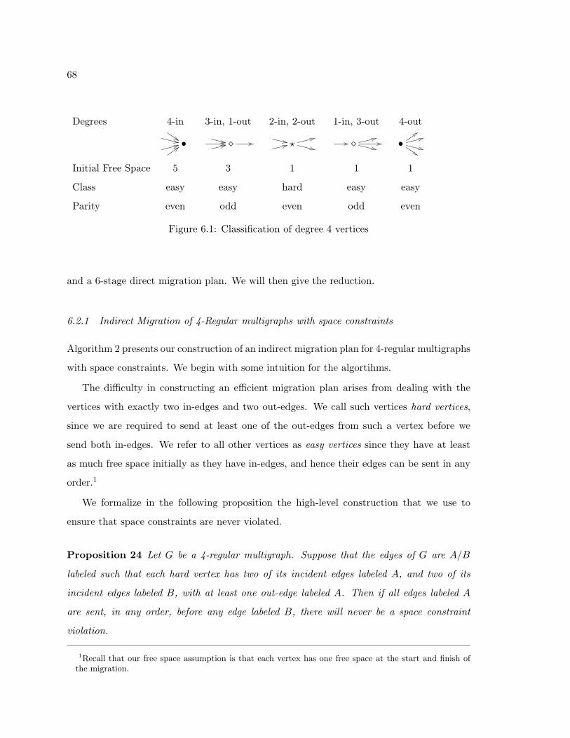
68
Degrees 4-in 3-in, 1-out 2-in, 2-out 1-in, 3-out 4-out
• •
Initial Free Space 5 3 1 1 1
Class easy easy hard easy easy
Parity even odd even odd even
Figure 6.1: Classification of degree 4 vertices
and a 6-stage direct migration plan. We will then give the reduction.
6.2.1 Indirect Migration of 4-Regular multigraphs with space constraints
Algorithm 2 presents our construction of an indirect migration plan for 4-regular multigraphs
with space constraints. We begin with some intuition for the algortihms.
The difficulty in constructing an efficient migration plan arises from dealing with the
vertices with exactly two in-edges and two out-edges. We call such vertices hard vertices,
since we are required to send at least one of the out-edges from such a vertex before we
send both in-edges. We refer to all other vertices as easy vertices since they have at least
as much free space initially as they have in-edges, and hence their edges can be sent in any
order.1
We formalize in the following proposition the high-level construction that we use to
ensure that space constraints are never violated.
Proposition 24 Let G be a 4-regular multigraph. Suppose that the edges of G are A/B
labeled such that each hard vertex has two of its incident edges labeled A, and two of its
incident edges labeled B, with at least one out-edge labeled A. Then if all edges labeled A
are sent, in any order, before any edge labeled B, there will never be a space constraint
violation.
1Recall that our free space assumption is that each vertex has one free space at the start and finish ofthe migration.

69
Algorithm 2 The bypass algorithm for 4-regular multigraphs. Given a 4-regular multigraph
with n nodes, this algorithm uses at most n/3 bypass nodes to color the multigraph with
exactly 4 colors in a way that respects space constraints.
1. Split each hard vertex into two representative vertices with one having two in-edges
and the other having two out-edges. This breaks the graph into connected components
(when the edges are viewed as undirected). (Figure 6.2(a) shows an example graph,
and Figure 6.2(b) shows the result of splitting hard vertices, shown as .)
2. Construct an Euler tour for each component (ignoring the directionalities of the edges)
(Figure 6.2(c) shows the resulting Euler tours.)
3. Alternately A/B label the edges along the Euler tour of each of the even components.
4. While there exist a pair of odd components that share a vertex (each component
contains one of the split hard vertices), label the two out-edges of the split vertex A,
label the two in-edges of the split vertex B, and alternately A/B label the remaining
portions of the two Euler tours. (Figure 6.2(d) shows an example.)
5. Repeatedly select an unlabeled odd component and perform the following step:
Within that component, bypass exactly one edge, say (u, v), where the edge is chosen
using Procedure 1. Label A the edge from u to the new bypass node and B the edge
from the bypass node to v. Alternately A/B label the remaining edges in the tour.
6. The resulting A and B subgraphs have maximum degree 2. (The only vertices in
either graph of degree 1 are bypass nodes.) Bypass an edge in each odd cycle that
occurs in either the A or B graph, converting all cycles to even-length cycles. The
graph can now be colored with 4 colors in a way that respects space constraints. We
simply alternately color the edges in each A cycle color 1 and color 2, and alternately
color the edges in the B cycle color 3 and color 4.
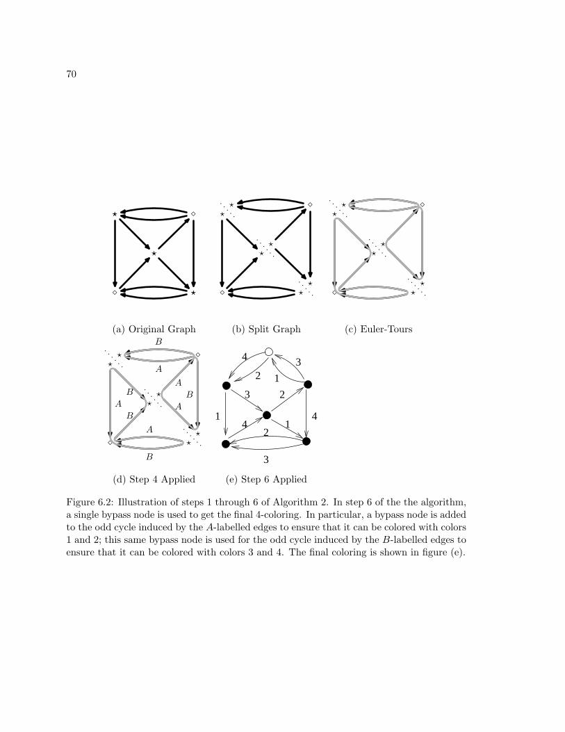
70
(a) Original Graph (b) Split Graph (c) Euler-Tours
B
A
A
B
A
A
B
B
A
B
1
3
2
41
2
4
3
4
23
1
(d) Step 4 Applied (e) Step 6 Applied
Figure 6.2: Illustration of steps 1 through 6 of Algorithm 2. In step 6 of the the algorithm,a single bypass node is used to get the final 4-coloring. In particular, a bypass node is addedto the odd cycle induced by the A-labelled edges to ensure that it can be colored with colors1 and 2; this same bypass node is used for the odd cycle induced by the B-labelled edges toensure that it can be colored with colors 3 and 4. The final coloring is shown in figure (e).

71
Thus, our goal is reduced to finding an A/B labeling that meets the conditions of
Proposition 24, and that can be performed in as few stages as possible.
Interestingly, if there are no odd vertices (shown in the figures as ), vertices such that
the parity of their in-degree (and out-degree) is odd, then the problem is easy: We split
each vertex into two with the property that each new vertex has exactly two edges of the
same orientation. This new graph need not be connected. We construct an Euler-tour of
each component (ignoring the directionality of the edges) and alternately label edges along
these tours A and B. No conflicts arise in the A/B labeling because the tours have even
length – each vertex has either only in-edges or only out-edges so the tour passes through
an even number of vertices. The A and B induced subgraphs are a 2-factor decomposition
of the original graph with the property that exactly one out-edge is labeled A. We can thus
use our standard method for performing migration with or without bypass nodes given a
2-factor decomposition. With bypass nodes, this method sends the A-edges in stages one
and two and the B-edges in stages three and four.
When there are both odd vertices and hard vertices, the problem becomes more difficult.
In particular, it is not hard to show that there exist 4-regular multigraphs in which no A/B
labeling of the graph ensures that every vertex has two incident A edges and two incident
B edges, with at least one A-labeled out-edge from each hard vertex. To solve the problem,
we will need to bypass some of the edges in the graph.
Our algorithm starts out very much like the algorithm just described for graphs with
no odd nodes, but now we split only the hard vertices into two representative vertices with
one having two in-edges and the other having two out-edges.
Each resulting component (disregarding edge directionality) still has an Euler tour of
course, but not all components have even length. We call those with even length tours
even components and those with odd length tours odd components. Those that do have
even length can be alternately A/B labeled. We could then bypass one edge in each odd
component, and A/B label the resulting even-length tour. Note that the choice of bypassed
edge determines the A/B labeling of the tour – as discussed in Section 6.1 the incoming
edge to the bypass node must be labeled A and the outgoing edge must be labeled B.
Unfortunately, this will not give us a good bound on bypass nodes, since there can be

72
2n/5 odd components (Figure 6.2). We get around this problem by observing that the
A/B labeling so constructed satisfies a more restrictive property than that needed to obey
space constraints – it guarantees that every hard vertex has both an in-edge and an out-edge
labeled A. This excludes perfectly legal labelings that have hard vertices with two out-edges
labeled A. Indeed, it is not possible in general to beat the 2n/5 bound on bypass nodes if
we disallow both out-edges from being labeled A.
Therefore, the algorithm will sometimes have to label both out-edges from a hard vertex
A. In our algorithm, this happens whenever we find a pair of odd components that share
representatives of the same hard vertex. We can merge the two odd components into a
single even component which can be A/B labeled such that both out-edges of the shared
hard vertex are labeled A. When no remaining unlabeled odd components can be merged
in this fashion, we are guaranteed that there are at most n/3 odd components remaining.
Unfortunately, our work is not done, since in addition to the bypass nodes introduced for
each remaining odd component (which have one incident edge labeled A and one incident
edge labeled B), there may be odd cycles in the A and B induced graphs. We will also need
to bypass one edge in each of these odd cycles. If we are not careful about which edge we
bypass in the odd component, we will end up with too many bypass nodes used to break
odd A or B cycles. The heart of our algorithm and analysis is judiciously choosing which
edge to bypass in each odd component. With carefully accounting for these bypass nodes
in the analysis, we show that the total number of bypass nodes used is at most n/3.
Terminology.
The result of steps 1-4 is a decomposition of the graph into a collection of unlabeled odd
components that are connected via A or B labeled paths (which correspond to edges that
were in even components, or odd components that were merged and labeled in Step 4)
Within each unlabeled odd component, we have two types of vertices: internal vertices,
which have all their edges inside the odd component, and external vertices, which have only
two edges, either both directed towards the vertex or both directed away from the vertex.
Since adjacent odd components have been labeled (Step 4), the other two edges incident to

73
C3
C2
C1
C4
External A loopExternal B path
Figure 6.3: An example of what the graph might look like after Step 4.
each external vertex are both already labeled (one A and one B).
Figure 6.3 shows a example of what the resulting graph might look like. There are
four unlabeled components (C1, . . . , C4). Classify the A and B paths emanating from each
external vertex as either an external loop if its two endpoints (external vertices) are in
the same unlabeled component, or as an external path if its two endpoints are in different
unlabeled components.
Analysis.
We now turn to the analysis of the algorithm. By construction, edges are A/B labeled so
that the conditions of Proposition 24 are met, and hence we have:
Lemma 25 Algorithm 2 computes a migration plan that respects space constraints.
Our main theorem is the following:

74
Procedure 1 A/B coloring odd componentsThere are two cases:
1. There is only one external vertex.
Within this case, there are two subcases:
• If there is a pair of internal vertices that are each not adjacent to the external
vertex that have an edge between them, bypass that edge.
• If not, there are only two possible graphs, shown below. We omit the justification
of this fact. (The external vertex is on the left and the directionality of the edges
is not shown.) Bypass the dashed edge.
2. There are 3 or more external vertices.
Let v be the external vertex incident to the largest number of external loops. Bypass
one of its incident internal edges. If the resulting A/B labeling of this component’s
Euler tour creates an A or B cycle with v (containing an external loop and an internal
path connecting the endpoints of the external loop), switch which one of v’s internal
edges is bypassed.

75
Theorem 26 The bypass algorithm for edge coloring 4-regular multigraphs with space con-
straints uses four colors and at most n/3 bypass nodes, where n is the number of nodes in
the graph.
Proof: By construction, the algorithm described uses 4 colors. We have only to show that
it uses at most n/3 bypass nodes. We do this by “crediting” each bypass node used in the
A stages with a distinct set of three vertices in the graph, and crediting each bypass node
used in the B stages with a distinct set of three vertices in the graph.
A bypass node that is created in order to break an odd A cycle (or B cycle) will be
credited with three vertices in that cycle. Notice that bypass nodes used to break A cycles
can be reused to break B cycles. The tricky part of the argument will be to show that each
bypass node that is created when an odd component is A/B labeled can also be credited
with 3 vertices.
The accounting scheme we use is based on the following observations about the structure
of what happens when step 5 is performed. Prior to performing this step, we have exactly
one A external path or loop and exactly one B external path or loop connected to each
external node. When we pick an edge inside the component to bypass, and A/B label
the component, every internal vertex (which is of degree 4) gets two of its incident edges
labeled A and two of its incident edges labeled B, and every external vertex gets one of
its incident internal edges labeled A and one labeled B. Thus the internal A path (or B
path) emanating from an external node either terminates at a bypass node, in which case
we call it an end path, or it terminates at another external node, in which case we call it an
inscribed path. Thus, looking at the A subgraph (or similarly the B subgraph) of an odd
component with 2k + 1 external vertices, we obtain precisely k disjoint inscribed A paths
and one A end path. (Note that the odd component must have an odd number of external
vertices, since each internal vertex appears twice in the Euler tour of the component and
each external vertex appears once and the length of the tour is odd.)
For the case where an odd component has exactly one external vertex, we can simply
verify that breaking the proposed edge results in three vertices not in odd cycles that can
be credited to the A and B end-path. In both graphs, bypassing any edge except the ones

76
incident to the external vertex guarantees that there will be no odd cycle created inside the
component. Since only the end paths leave the components all vertices inside the component
are not in odd cycles and can be credited to the bypass node.
If the odd component has more than one external vertex, then it must have at least
three. We will credit the bypass node with the external node on the end path terminating
at the bypass node (which in general will be different for A and B), and with two other
external vertices in the component. The difficulty is that if we are not careful about which
edge in the component we bypass, the two other external vertices we select can have an
inscribed A path between them and an external A loop, and thus might end up in a short
odd A cycle. If this happens, we will violate our condition of crediting each bypass node
with distinct vertices in the graph, since the bypass node created to break this short A cycle
will also be credited with these vertices. Therefore, we choose an edge to bypass so that the
other two external vertices we credit to the bypass node are not in a short cycle.
We find that it is sufficient to guarantee that for each odd component processed in Step 5,
in the resulting A graph (resp. in the resulting B graph) one of the following situations holds:
1. There are at least two external paths labeled A (resp. B).
If there are at least two external paths labeled A, one of them is not connected to the
A end path. Thus, there is an inscribed A path that connects the external path to
some other external path or loop. In this case, we credit the bypass node (in stage A)
with the two external vertices on this inscribed path and with the external vertex on
the A end path connected to it.
2. The component is labeled so that there is an A (resp. B) external loop that does not
form a cycle with an inscribed A (resp. B) path.
In this case, the A external loop is connected to some other A external loop or path via
an inscribed A path. We can again credit the bypass node with the external vertices
on this inscribed path and with the external vertex on the end path connected to it.
If the edge selected to bypass in Step 5 results in one of these two situations holding, we
say that a good edge was bypassed.

77
Notice that in both of these situations, the two external vertices credited to the bypass
node may end up in an odd A (or B) cycle. We claim, however, that if this happens, it is an
odd cycle created by two or more external A loops or paths and hence it has length at least
five. Since we have only credited two of the external vertices on the cycle to the bypass
node created in Step 5, we still have three vertices in the odd cycle that can be credited to
the bypass node that will be used to break the cycle. In fact, the argument is slightly more
complicated than this – we omit the details.
Finally, we must show that the procedure used to select an edge to bypass in each odd
component with at least three external vertices results in bypassing a good edge.
Let v be the odd component’s external vertex with the largest number of incident ex-
ternal loops as chosen by the algorithm. If there is no external A (likewise B) loop at v
then the odd component has at least two A paths and, as such, any edge is good for A. To
see why this is the case note that if v has no external loops then no external vertices have
loops so clearly there are at least two external paths of both labels. If v has one external
loop of label B then the other endpoint of the loop has a B loop (the same one). Since v
has the largest number of loops, this other vertex can not have an A loop. Thus, both this
vertex and v have A paths.
Now we argue that our choice of edge to bypass guarantees that any external loop
emanating from v does not form a cycle with an inscribed path. Suppose v’s internal edges
are both in-edges2 from vertices u1 and u2 and we bypass the edge (u1, v) using bypass node
b. The edges (u1, b) and (u2, v) are thus both labeled A and the edge (b, v) is labeled B
(See Figure 6.4(b)). As such the B loop, if there is one, does not create a cycle. Assume
that there is an A loop. If not, we are done. If labeling the rest of the odd component
according the the Euler tour does not cause an incribed path to be created between the
external A loop’s endpoints then we are also done and (u1, v) is good for A. Otherwise,
this incribed path must go through the edge (u2, v). The algorithm swaps which edge is
bypassed so that edges (u2, b) and (u1, v) are both labeled A and the edge (b, v) is labeled B
(See Figure 6.4(c)). The bypassed edge is still good for B. We now argue that is also good
2The case where they are both out-edges is similar.
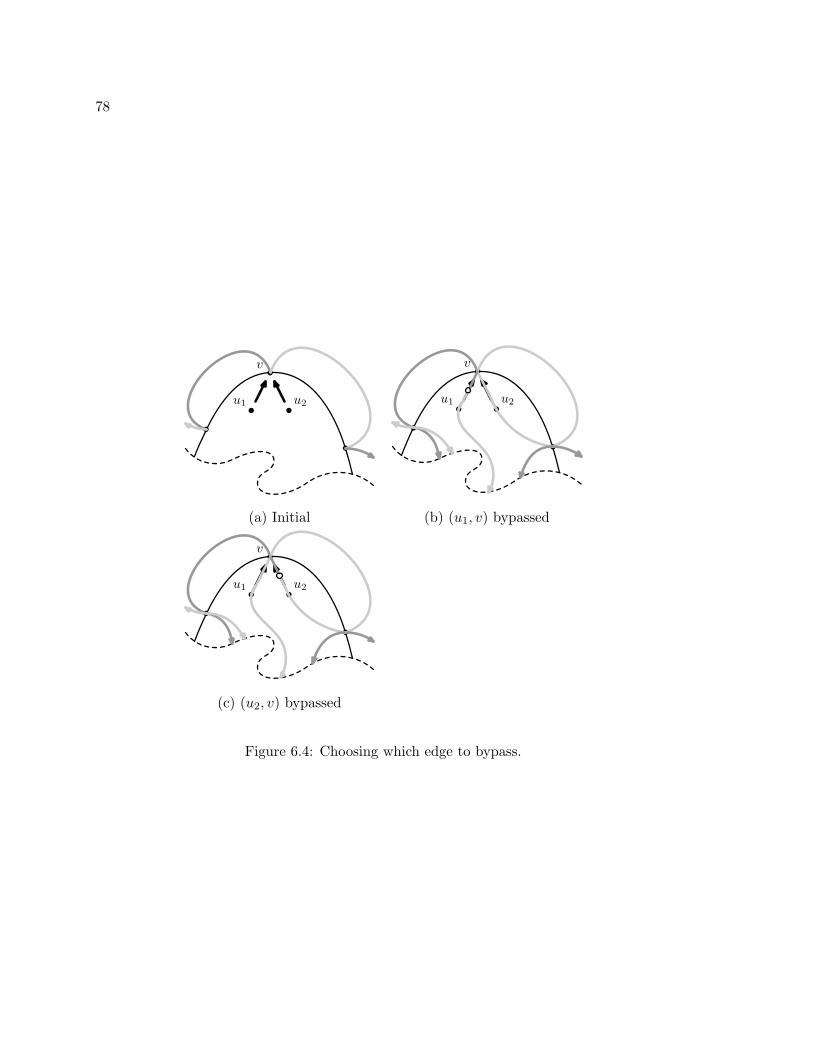
78
v
u1 u2
v
u1 u2
(a) Initial (b) (u1, v) bypassed
v
u1 u2
(c) (u2, v) bypassed
Figure 6.4: Choosing which edge to bypass.

79
for A. The rest of the labeling remains the same as the edges incident on u1 and u2 have
not changed labels. Since the rest of the labeling does not change, there is still an internal
A path from the one endpoint of the external A loop to u2. This path continues from u2 to
b and terminates. Thus, the edge (u2, v) is good for A.
6.2.2 4-regular migration without bypass nodes
We next show how to compute a six stage migration plan of a 4-regular multigraph without
using bypass nodes. The first 4 steps of the algorithm are the same as in Algorithm 2.
Procedure 2 replaces Steps 5 and 6 of Algorithm 2, the only steps that used bypass nodes,
with a construction that uses two extra colors instead. In this procedure, the label A will
be for stages 1, 2, and 3, while the label B will be for stages 4, 5, and 6.
After completing Step 4 of the previous algorithm, the graph contains a number of
unlabeled disjoint odd components connected by A/B labeled paths and loops (Figure 6.3).
We make the following additional observations about the graph:
• Each odd component contains at least one odd vertex. (Otherwise, the tour would be
of even length.)
• Since odd unlabeled components are disjoint, and odd vertices are always internal,
every path between two odd vertices in different odd unlabeled components has length
at least three.
The algorithm can be easily seen to meet the conditions of Proposition 24. Straightfor-
ward arguments thus give us the following theorem:
Theorem 27 The above algorithm computes a proper six coloring of the graph that respects
the space constraints of the hard vertices.
Proof: First we argue that the coloring is proper. For the A induced subgraph, this is
immediate. For the B induced subgraph, the the argument is not as straightforward. First,

80
Procedure 2 Final steps in 4-regular migration without bypass nodes
5′. A/B label each remaining odd component by starting with an odd vertex, v, and the
label B and following the Euler tour of the component labeling edges alternately A
and B. Note: v will have three B labeled edges incident and one A labeled edge.
6′. Color the A and B induced subgraphs:
(a) Color the A induced subgraph (note: the A induced subgraph is a set of paths
and cycles):
i. Break all odd length cycles by coloring one edge in them 3.
ii. Color all remaining paths and even cycles with the colors 1 and 2.
(b) Color the B induced subgraph (note: the B induced subgraph has vertices of
degree two and degree three only):
i. Color one edge 6 on each degree three vertex. We are left with cycles and
paths.
ii. Color one edge 6 in each odd length cycle to convert the cycle into a path.
Choose an edge that is not incident on one of the degree three vertices (which
is possible because of the second observation above).
iii. The remaining graph is just paths and even cycles. Color them with colors
4 and 5.

81
the path distance between any two degree three vertices in the B subgraph is at least three.
This is because they are odd nodes from different odd components that are not adjacent.
This means that they do not share neighbors so they must have two vertices between them
(and thus three edges). Since this is the case, step 6′(b)i of Procedure 2 does not color two
edges 6 that are incident on the same vertex. Also because of the distance between degree
three vertices in the remaining odd cycles there must be an edge that is not incident on
a degree three vertex. As such step 6′(b)ii does not color an edge 6 that is incident to a
vertex that already has a 6 edge. It is easy to see that colors 4 and 5 are proper.
Now we argue that space constraints are respected. Since all edges in the A subgraph
are sent before all edges in the B subgraph, all we have to show is that each hard vertex
has an A colored out-edge. In Step 5′ we colored alternating edges A and B in the Euler
tour of each odd component. Since hard nodes are split into two representatives such that
each representative has either two in-edges or two out-edges, the alternating Euler tour will
color one in-edge and one out-edge A and and likewise for B. Having consecutive Bs on an
odd vertex in the tour does not affect the hard vertices. As such each hard vertex in the
remaining components has an A colored out-edge. By the correctness of the previous steps
of the algorithm, all vertices previously A/B colored have this property as well.
6.2.3 The Reduction
We next show how to reduce the general migration problem with space constraints to the
problem of migration with space constraints on 4-regular multigraphs. Ideally, we might
like to split the graph into 2-factors, such that sending the edges within a 2-factor in any
order satisfies our space constraints, and so that after each 2-factor is sent, there is still one
free space at each vertex. This is not always possible. What we are able to do is to split the
graph into 4-factors such that after each 4-factor is sent, there is once again a free space at
each vertex. To partition the edges of the graph in this way, we need, roughly speaking, to
match up in-edges of a vertex with corresponding out-edges. Algorithm 3 gives the precise
details.

82
The key lemma is the following:
Lemma 28 A migration that repeatedly picks one edge incident to vin and one incident to
vout to send in either order will never violate the space constraints of v.
Proof: We consider two cases, depending on which of vin or vout has incident edges only of
one type (at least one of them must).
Case: vout has only incident out-edges.
Then since one of the edges chosen is an out-edge there will be at least one out-edge
sent for every in-edge so the free space after the two edges are sent is at least what it
was before.
Case: vin has only incident in-edges.
If = din − dout, then we know by the free space assumption that there are at least
+ 1 free spaces initially. We allocate this free space as follows:
• The number of times that two in-edges are chosen is exactly /2 we allocate two
free spaces to each of these.
• The remaining times we choose an in-edge and an out-edge. All of these cases
will share the one remaining free-space. Since both an in-edge and an out-edge
are sent, we will regain the free space again after the two edges are sent.
Note that since we always have exactly one edge incident to vin and exactly one incident
to vout if the edge happens to be a dummy self loop then it is the only edge chosen at this
step of the migration. Since nothing happens in this case, the available free space remains
unchanged. There is also at most one dummy edge and it is incident to vin or vout, whichever
has less of its type of edge. Our argument above focused on the edges incident on vin or
vout, whichever has more of its type of edge, so the arguments still hold when a dummy
edge is present.

83
Algorithm 3 The reduction to 4-regular graphs
1. Make G regular with degree a multiple of four (4k) (using the procedure in Sec-
tion 6.3.1).
2. Split each vertex v into vin and vout assigning v’s edges to either vin or vout to get G′
as follows:
(a) Assign dummy self loops, (v, v), as (vout, vin).
(b) Assign the remaining in-edges to vin and the remaining out-edges to vout (exclud-
ing the dummy edge).
(c) Assign the dummy edge, if there is one, to the representative of v with the least
number of adjacent edges.
(d) Make the degrees of vin and vout equal by moving real edges from one to the
other until they have equal degree.
G′ has 2n vertices and is 2k-regular.
3. Compute a 2-factoring of G′ (viewed as undirected). This gives k 2-factors.
4. In each 2-factor merge vertex representatives back together. That is, vin and vout
become v again. The result is k 4-factors of our original graph G. The problem is
thus reduced to computing a migration with space constraints on these 4-factors of G.
84
We thus obtain:
Theorem 29 Algorithm 3 reduces the problem of performing a migration with space con-
straints on an arbitrary graph to that of performing a series of migrations with space con-
straints on 4-regular multigraphs.
6.2.4 The Algorithms 4-Factoring Direct and 4-Factoring Indirect
We can now define the algorithms 4-Factoring Direct and 4-Factoring Indirect.
The algorithm 4-Factoring Direct is defined as follows: Use Algorithm 3 to reduce the
graph into 4-factors and then use the algorithm from Theorem 27(in Section 6.2.2) to migrate
each of these in 6 steps.
The algorithm 4-Factoring Indirect is defined as follows: Use Algorithm 3 to reduce the
graph into 4-factors and then use the algorithm 2 to migrate each of these in 4 steps using
no more than n/3 bypass nodes.
Combining Theorem 29 with Theorems 27 and 26 gives us the following corollaries:
Corollary 30 4-Factoring Direct takes as input an arbitrary directed multigraph of maxi-
mum degree ∆ and finds a 6 ∆/4 stage migration plan without bypass nodes.
Corollary 31 4-Factoring Indirect takes as input an arbitrary directed multigraph of max-
imum degree ∆ and finds a 4 ∆/4 stage migration plan using at most n/3 bypass nodes.
6.3 Obtaining a Regular Graph and Decomposing a Graph
6.3.1 Obtaining a Regular Graph
Some of our algorithms require regular graphs of degree either a multiple of 2 or 4. Let
∆′ be this desired degree, either 2 ∆/2 or 4 ∆/4. We construct such directed regular
multigraphs as follows.

85
Algorithm 4 Making a directed multigraph ∆′-regular for any even ∆′
1. While there exists a vertex with degree less than ∆′−1, add a self loop to that vertex.
2. While there exist two distinct vertices of degree ∆′ − 1, add an arbitrarily directed
edge between them.
6.3.2 2-factor decomposition
It is well known that a 2k-regular multigraph can be factored into k 2-factors. For complete-
ness, we review an algorithm for doing this. This algorithm takes an undirected multigraph
G with degree ∆ = 2k and returns k 2-factors of G. We will be performing this operation
on directed multigraphs. In this case, the directions of the edges are ignored during the
factoring algorithm.
Algorithm 5 2-factoring a multigraph
1. Construct an Euler-tour of G.
2. Orient the edges according to the direction of the tour. That is, if the tour enters v
on edge e1 and leaves on edge e2, then e1 is an in-edge to v and e2 is an out-edge.
Thus we have din = dout = k.
3. Set up a bipartite matching problem, BG, with a representative of each vertex in the
graph on both sides. Add in all directed edges going from left to right. Note that
each edge is represented it the matching problem exactly once.
4. Find a matching (which is guaranteed to exist by Hall’s Theorem). The matched
edges induce a 2-factor of the original graph. Remove these edges from BG and repeat
this step until there are no edges left.
86
Chapter 7
EXPERIMENTAL STUDY OF DATA MIGRATION ALGORITHMS
FOR IDENTICAL DEVICES AND COMPLETE TOPOLOGIES
The primary focus of the chapter is on the empirical evaluation of the algorithms from
the last chapter along with two new migration algorithms. The chapter is organized as
follows. In Section 7.1, we describe the algorithms we have evaluated for indirect migration
without space constraints. In Section 7.2, we describe the algorithms we have evaluated for
migration with space constraints. Section 7.3 describes how we create the demand graphs on
which we test the migration algorithms while Sections 7.4 and 7.5 describe our experimental
results. Section 7.6 gives an analysis and discussion of these results.
7.1 Indirect Migration without Space Constraints
We begin with the new algorithm, Max-Degree-Matching given as Algorithm 6. Max-Degree-
Matching uses at most 2n/3 bypass nodes and always attains an optimal ∆ step migration
plan without space constraints. The algorithm works by sending, in each stage, one object
from each vertex in the demand graph that has maximum degree. To do this, we first find
a matching which matches all maximum-degree vertices with no out-edges. Next, we use
the general matching algorithm [MV80] to expand this matching to a maximal matching.
Finally, we match each unmatched maximum-degree vertex up with a bypass node and
then send every edge in this final matching. Theorem 32 gives the main properties of the
algorithm.
Theorem 32 Max-Degree-Matching computes a correct ∆-stage migration plan using at
most 2n/3 bypass nodes.
Proof: First we show that the algorithm uses no more than ∆ stages. Hall’s theorem can
be used to show that the matching problem constructed in step 1 of the algorithm always

87
Algorithm 6 Max-Degree-Matching(demand graph G)
1. Set up a bipartite matching problem as follows: the left hand side of the graph is
all maximum degree vertices not adjacent to degree one vertices in G, the right hand
side is all their neighbors in G, and the edges are all edges between maximum degree
vertices and their neighbors in G .
2. Find the maximum bipartite matching. The solution induces cycles and paths in the
demand graph. All cycles contain only maximum degree vertices, all paths have one
endpoint that is not a maximum degree vertex.
3. Mark every other edge in the cycles and paths. For odd length cycles, one vertex will
be left with no marked edges. Make sure that this is a vertex with an outgoing edge
(and thus can be bypassed if needed). Each vertex has at most one edge marked.
Mark every edge between a maximum degree vertex and a degree one vertex.
4. Let V ′ be the set of vertices incident to a marked edge. Compute a maximum matching
in G that matches all vertices in V ′ (This can be done by seeding the general matching
algorithm [MV80] with the matching that consists of marked edges.) Define S to be
all edges in the matching.
5. For each edge vertex u of maximum degree with no incident edge in S, let (u, v) be
some out-edge from u. Add (u, b) to S, where b is an unused bypass node, and add
(b, v) to the demand graph G.
6. Schedule all edges in S to be sent in the next stage and remove these edges from the
demand graph.
7. If there are still edges in the demand graph, go back to step 1.

88
has a solution in which all the maximum degree vertices not adjacent to degree 1 vertices
are matched. Thus at each stage the degree of each maximum degree vertex is decreased by
one. After ∆ stages we have no edges left and are done. The constraint that each vertex has
only one edge sent or received per stage is maintained because we only send the edges in a
general matching solution and edges out of vertices not matched by the general matching.
Next we show that the algorithm uses no more than 2n/3 bypass nodes. We first note
that there are no more than n/2 active bypass nodes after each stage. Then we show that
in the turnover as some bypass nodes are spent and some are created within a stage, that
the number of bypass nodes does not exceed 2n/3. We wish to show that after each stage
in the bypass algorithm, only n/2 bypass nodes are in use. Let k be the number of paths
and cycles induced in G by the matching. After this stage each component can only have
one bypass node associated with it. For cycles this is because originally the cycle had no
bypass nodes, but if it is an odd cycle then after this stage it has one bypass node. For
paths this is because any odd length path could end in a node with a bypass node. If this
is the case, since the path is odd length, the bypass node does not get used. Each of these
path or cycle has at least two vertices, so k ≤ n/2. Any bypass node that is not adjacent
to a path or cycle will be satisfied in this stage. Thus, there are at most n/2 bypass nodes
after any stage. Note that this says nothing about the number of different bypass nodes
used in a stage. For example, the bypass nodes at the end of the stage might not be the
same as the ones at the start of the stage. If one node is used in a stage and one node is
created, two nodes must exist because the node cannot both send (to be used) and receive
(to be created) in the same stage.
To get the bound on the number of nodes in use during a given stage of less than 2n/3,
we note that we need to bound the sum of the number of bypass nodes enlisted in this
stage and the number that were left from the previous stage. Assume the number of bypass
nodes left over from the previous stage is nb, and that the number of maximum degree
vertices without bypass nodes is nm. The number of bypass nodes created in this stage
is bounded by nm/3 because bypass nodes are only created from odd length cycles in the
matching. These cycles must have at least 3 vertices in them and only vertices not adjacent
to bypass nodes (ones put on the left hand side of the matching) can be in cycles in the
89
matching. Here, nm is at at most n − nb because each bypass node is adjacent to exactly
one maximum degree node. So to maximize the number of bypass nodes we must maximize:
nm/3 + nb ≤ (n − nb)/3 + nb = n/3 + 2nb/3. We proved above that nb ≤ n/2 so the most
bypass nodes that can be in use during a given stage is 2n/3. Bypass nodes can be recycled
so that only 2n/3 are required for the entire bypass algorithm.
We compare Max-Degree-Matching with 2-factoring, which also computes an indirect
migration plan without space constraints. We have shown in the last chapter that 2-factoring
takes 2 ∆/2 time steps while using no more than n/3 bypass nodes.
We note that in a particular stage of 2-factoring as described in the last chapter, there
may be some nodes which only have dummy edges incident to them. A heuristic for reducing
the number of bypass nodes needed is to use these nodes as bypass nodes when available to
decrease the need for “external” bypass nodes. Our implementation of 2-factoring uses this
heuristic.
7.2 Migration with Space Constraints
The Greedy Matching algorithm (Algorithm 7) is a new and straightforward direct migration
algorithm which obeys space constraints. This algorithm eventually sends all of the objects
(see Section 7.2.1) but the worst case number of stages is unknown.
7.2.1 Proof of Termination for Greedy Matching
For a node v, let din(v) be the in-degree of the node and let dout(v) be the out degree.
Lemma 33 Given initial free space of fi ≥ 1 + max(0, din(vi) − dout(vi)), at any stage of
Greedy Matching (i.e. after sending any number of objects) at least one unsent object is
sendable.
Proof: At any stage in the migration, the graph G only has edges left in it for objects that
have not yet been sent to their destination. Since we assume that fi ≥ 1 + max(0, din(vi)−
dout(vi)) for all i initially, all we have to show now, is that there exists a node v∗ ∈ V that

90
Algorithm 7 Greedy Matching
1. Let G′ be the graph induced by the sendable edges in the demand graph. An edge is
sendable if there is free space at its destination.
2. Compute a maximum general matching on G′.
3. Schedule all edges in matching to be sent in this stage.
4. Remove these edges from the demand graph.
5. Repeat until the demand graph has no more edges.
has din(v∗)− dout(v∗) ≥ 0 with din(v∗) > 0. This would imply that v∗ has free space and an
incoming edge and hence the object corresponding to that incoming edge is sendable.
Let V ′ be the subset of V that has only vertices that have sendable edges (that is,
din + dout > 0). Then∑
v∈V ′ (din(v) − dout(v)) = 0. This is because each edge contributes
to exactly one vertex’s in-degree and one vertex’s out-degree. Since the average over all
v ∈ V ′ of (din(v) − dout(v)) = 0, there must be a vertex in V ′, which we call v∗, with
din(v∗) − dout(v∗) ≥ 0. Since we also have dout(v∗) ≥ 0, it must be that din(v∗) > 0.
We compare Greedy-Matching with the two provably good algorithms for migration with
space constraints from the last chapter: 4-factoring direct and 4-factoring indirect. We have
shown that 4-factoring direct finds a 6 ∆/4 stage migration without bypass nodes and that
4-factoring indirect finds a 4 ∆/4 stage migration plan using at most n/3 bypass nodes.
In our implementation of 4-factoring indirect, we again use the heuristic of using nodes
with only dummy edges in a particular stage as bypass nodes for that stage.

91
Table 7.1: Theoretical Bounds for Tested Migration Algorithms
Algorithm Type Space Constraints Plan Length Worst Case
Max. Bypass Nodes
2-factoring indirect No 2 ∆/2 n/3
4-factoring direct direct Yes 6 ∆/4 0
4-factoring indirect indirect Yes 4 ∆/4 n/3
Max-Degree-Matching indirect No ∆ 2n/3
Greedy-Matching direct Yes unknown 0
7.3 Experimental Setup
Table 7.1 summarizes the theoretical results known for each algorithm on which we have
run experiments1.
We tested these algorithms on four types of multigraphs2:
1. Load-Balancing Graphs. These graphs represent real-world migrations. A detailed
description of how they were created is given in Section 7.3.1.
2. General Graphs(n, m). A graph in this class contains n nodes and m edges. The edges
are chosen uniformly at random from among all possible edges disallowing self-loops
(but allowing parallel edges).
3. Regular Graphs(n, d). Graphs in this class are chosen uniformly at random from
among all regular graphs with n nodes, where each node has total degree d (where
d is even). We generated these graphs by taking the edge-union of d/2 randomly
generated 2-regular graphs over n vertices.
1For each algorithm, the time to find a migration plan is negligible compared to time to implement theplan.
2Java code implementing these algorithms along with input files for all the graphs tested is available atwww.cs.washington.edu/homes/saia/migration
92
4. Zipf Graphs(n, dmin). These graphs are chosen uniformly at random from all graphs
with n nodes and minimum degree dmin that have Zipf degree distribution i.e. the
number of nodes of degree d is proportional to 1/d. Our technique for creating random
Zipf graphs is given in detail in Section 7.3.2 .
7.3.1 Creation of Load-balancing Graphs
A migration problem can be generated from any pair of configurations of objects on nodes
in a network. To generate the Load-Balancing graphs, we used two different methods of
generating sequences of configurations of objects which might occur in a real world system.
For each sequence of say l configurations, C1, . . . Cl, for each i, 1 ≤ i ≤ l − 1, we generate a
demand graph using Ci as the initial configuration and Ci+1 as the final.
For the first method, we used the Hippodrome system on two variants of a retail data
warehousing workload [AHK+01]. Hippodrome adapts a storage system to support a given
workload by generating a series of object configurations, and possibly increasing the node
count. Each configuration is better at balancing the workload of user queries for data objects
across the nodes in the network than the previous configuration. We ran the Hippodrome
loop for 8 iterations (enough to stabilize the node count) and so got two sequences of 8
configurations. For the second method, we took the 17 queries to a relational database
in the TPC-D benchmark [Cou96] and for each query generated a configuration of objects
to devices which balanced the load across the devices effectively. This method gives us a
sequence of 17 configurations.
Different devices have different performance properties and hence induce different config-
urations. When generating our configurations, we assumed all nodes in the network were the
same device. For both methods, we generated configurations based on two different types
of devices. Thus for the Hippodrome method, we generated 4 sequences of 8 configurations
(7 graphs) and for the TPC-D method, we generated 2 sequences of 17 configurations (16
graphs) for a total of 60 demand graphs.

93
7.3.2 Creation of Zipf Graphs
The Zipf graphs for mimimum degree dmin are generated as follows: we first create sets
S1, . . . , Sk each containing k! vertices and let S be the union of all the sets. We then find
dmin random perfect matchings from S to S so that now every vertex in S has degree dmin.
We next, for all i, 1 ≤ i ≤ k, partition Si into k!/i subsets each with i nodes and then
merge each of these subsets into one node. By doing this, we get k!/i new vertices each
with degree dmin ∗ i. We let these new vertices be the vertices of the Zipf graph.
The total number of vertices in this Zipf graph is k!Hk where Hk is the k-th Harmonic
number. We note that the maximum degree of the graph is dmin ∗ k while the minimum
degree is 1. We further note that for all i, 1 ≤ i ≤ dmin ∗k, the number of nodes with degree
i is dmin ∗ k!/i
7.4 Results on the Load-Balancing Graphs
7.4.1 Graph Characteristics
In this section, we describe the load-balancing graphs used in our experiments. We refer to
the sets of graphs generated by Hippodrome on the first and second device type as the first
and second set respectively and the sets of graphs generated with the TPC-D method for
the first and second device types as the third and fourth sets.
The number of nodes in each graph is less than 50 for the graphs in all sets except the
third in which most graphs have around 300 nodes. The edge density for each graph varies
from about 5 for most graphs in the third set to around 65 for most graphs in the fourth
set. The ∆ value for each graph varies from about 15 to about 140, with almost all graphs
in the fourth set having density around 140.
7.4.2 Performance
Figure 7.1 shows the performance of the algorithms on the load-balancing graphs in terms
of the number of bypass nodes used and the time steps taken. The x-axis in each plot gives
the index of the graph which is consistent across both plots. The indices of the graphs are

94
clustered according to the sets the graphs are from with the first, second, third and fourth
sets appearing left to right, separated by solid lines.
The first plot shows the number of bypass nodes used by 2-factoring, 4-factoring in-
direct and Max-Degree-Matching. We see that Max-Degree-Matching uses 0 bypass nodes
on most of the graphs and never uses more than 1. The number of bypass nodes used
by 2-factoring and 4-factoring indirect are always between 0 and 6, even for the graphs
with about 300 nodes. The second plot shows the number of stages required divided by
∆ for Greedy-Matching. Recall that this ratio for 2-factoring,Max-Degree-Matching and 4-
factoring indirect is essentially 1 while the ratio for 4-factoring direct is essentially 1.5. In
the graphs in the second and third set, Greedy-Matching almost always has a ratio near 1.
However in the first set, Greedy-Matching has a ratio exceeding 1.2 on several of the graphs
and a ratio of more than 1.4 on one of them. In all cases, Greedy-Matching has a ratio less
than 4-factoring direct.
We note the following important points: (1) On all of the graphs, the number of bypass
nodes needed is less than 6 while the theoretical upper bounds are significantly higher. In
fact, Max-Degree-Matching used no bypass nodes for the majority of the graphs (2) Greedy-
Matching always takes fewer stages than 4-factoring direct.
7.5 Results on General, Regular and Zipf Graphs
7.5.1 Bypass Nodes Needed
For General, Regular and Zipf Graphs, for each set of graph parameters tested, we generated
30 random graphs and took the average performance of each algorithm over all 30 graphs.
For this reason, the data points in the plots are not at integral values. Greedy-Matching
never uses any bypass nodes so in this section, we include results only for Max-Degree-
Matching, 4-factoring indirect and 2-factoring.
Varying Number of Nodes
The three plots in the left column of Figure 7.2 give results for random graphs where the
edge density is fixed and the number of nodes varies. The first plot in this column shows
95
0
1
2
3
4
5
6
7
0 10 20 30 40 50 60 70
Byp
ass
node
s re
quire
d
Graph number
Bypass nodes required for each demand graph
2-factoring4-factoring indirect
Max-Degree-Matching
1
1.1
1.2
1.3
1.4
1.5
1.6
1.7
1.8
0 10 20 30 40 50 60 70
stag
es r
equi
red/
delta
Graph number
Stages required/delta for each demand graph
Greedy Matching
Figure 7.1: Bypass nodes and time steps needed for the algorithms. The top plot givesthe number of bypass nodes required for the algorithms 2-factoring, 4-factoring indirectand Max-Degree-Matching on each of the Load-Balancing Graphs. The bottom plot givesthe ratio of time steps required to ∆ for Greedy-Matching on each of the Load-BalancingGraphs. The three solid lines in both plots divide the four sets of Load-Balancing Graphs

96
the number of bypass nodes used for General Graphs with edge density fixed at 10 as
the number of nodes increases from 100 to 1200. We see that Max-Degree-Matching and
2-factoring consistently use no bypass nodes. 4-factoring indirect uses between 2 and 3
bypass nodes and surprisingly this number does not increase as the number of nodes in the
graph increases.
The second plot shows the number of bypass nodes used for Regular Graphs with ∆ = 10
as the number of nodes increases from 100 to 1200. We see that the number of bypass nodes
needed by Max-Degree-Matching stays relatively constant at 1 as the number of nodes
increases. The number of bypass nodes used by 2-factoring and 4-factoring indirect are very
similar, starting at 3 and growing very slowly to 6, approximately linearly with a slope of
1/900.
The third plot shows the number of bypass nodes used on Zipf Graphs with minimum
degree 1 as the number of nodes increases. In this graph, 2-factoring is consistently at 0,
Max-Degree-Matching varies between 1/4 and 1/2 and 4-factoring indirect varies between 1
and 4.
Varying Edge Density
The three plots in the right column of Figure 7.2 show the number of bypass nodes used
for graphs with a fixed number of nodes as the edge density varies. The first plot in the
column shows the number of bypass nodes used on General Graphs, when the number of
nodes is fixed at 100, and edge density is varied from 20 to 200. We see that the number of
bypass nodes used by Max-Degree-Matching is always 0. The number of bypass nodes used
by 2 and 4-factoring indirect increases very slowly, approximately linearly with a slope of
about 1/60. Specifically, the number used by 2-factoring increases from 1/2 to 6 while the
number used by 4-factoring indirect increases from 4 to 6.
The second plot shows the number of bypass nodes used on Regular Graphs, when the
number of nodes is fixed at 100 and ∆ is varied from 20 to 200. The number of bypass
nodes used by Max-Degree-Matching stays relatively flat varying slightly between 1/2 and
1. The number of bypass nodes used by 2-factoring and 4-factoring indirect increases near

97
linearly with a larger slope of 1/30, increasing from 4 to 12 for 2-factoring and from 4 to 10
for 4-factoring indirect.
The third plot shows the number of bypass nodes used on Zipf Graphs, when the number
of nodes is fixed at 146 and the minimum degree is varied from 1 to 10. 2-factoring here
again always uses 0 bypass nodes. The Max-Degree-Matching curve again stays relatively
flat varying between 1/4 and 1. 4-factoring indirect varies slightly, from 2 to 4, again near
linearly with a slope of 1/5.
We suspect that our heuristic of using nodes with only dummy edges as bypass nodes
in a stage helps 2-factoring significantly on Zipf Graphs since there are so many nodes with
small degree and hence many dummy self-loops.
7.5.2 Time Steps Needed
For General and Regular Graphs, the migration plans Greedy-Matching found never took
more than ∆ + 1 time steps. Since the other algorithms we tested are guaranteed to have
plans taking less than ∆ + 3, we present no plots of the number of time steps required for
these algorithms on General and Regular Graphs.
As shown in Figure 7.3, the number of stages used by Greedy-Matching for Zipf Graphs
is significantly worse than for the other types of random graphs. We note however that
it always performs better than 4-factoring direct. The first plot shows that the number of
extra stages used by Greedy-Matching for Zipf Graphs with minimum degree 1 varies from 2
to 4 as the number of nodes varies from 100 to 800. The second plot shows that the number
of extra stages used by Greedy-Matching for Zipf Graphs with 146 nodes varies from 1 to 11
as the minimum degree of the graphs varies from 1 to 10. High density Zipf graphs are the
one weakness we found forGreedy-Matching.
7.6 Analysis
Our major empirical conclusions for the graphs tested are:
• Max-Degree-Matching almost always uses less bypass nodes than 2-factoring.

98
0
0.5
1
1.5
2
2.5
3
3.5
4
0 200 400 600 800 1000 1200
Byp
ass
node
s
Number of Nodes
General Graph, Density = 10
’2-factoring’’4-factoring indirect’
’Max-Degree-Matching’
0
2
4
6
8
10
12
14
0 20 40 60 80 100 120 140 160 180 200
Byp
ass
node
s
Density
General Graph, Nodes = 100
’2-factoring’’4-factoring indirect’
’Max-Degree-Matching’
0
1
2
3
4
5
6
7
8
0 200 400 600 800 1000 1200
Byp
ass
node
s
Number of Nodes
Regular Graph, Delta = 10
’2-factoring’’4-factoring indirect’
’Max-Degree-Matching’
0
2
4
6
8
10
12
14
0 20 40 60 80 100 120 140 160 180 200
Byp
ass
node
s
Delta
Regular Graph, Nodes = 100
’2-factoring’’4-factoring indirect’
’Max-Degree-Matching’
0
1
2
3
4
5
0 100 200 300 400 500 600 700
Byp
ass
node
s
Number of Nodes
Zipf Graph, Minimum Degree = 1
’2-factoring’’4-factoring indirect’
’Max-Degree-Matching’
0
1
2
3
4
5
6
1 2 3 4 5 6 7 8 9 10
Byp
ass
node
s
Minimum Degree
Zipf Graph, Nodes = 147
’2-factoring’’4-factoring indirect’
’Max-Degree-Matching’
Figure 7.2: Six plots giving the number of bypass nodes needed for 2-factoring, 4-factoringdirect and Max-Degree-Matching for the General, Regular and Zipf Graphs. The three plotsin the left column give the number of bypass nodes needed as the number of nodes in therandom graphs increase. The three plots in the right column give the number of bypassnodes needed as the density of the random graphs increase. The plots in the first row arefor General Graphs, plots in the second row are for Regular Graphs and plots in the thirdrow are for Zipf Graphs.
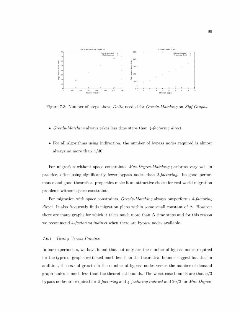
99
0
10
20
30
40
50
60
70
80
0 100 200 300 400 500 600 700
Ste
ps n
eede
d ab
ove
Del
ta
Number of Nodes
Zipf Graph, Minimum Degree = 1
’Greedy Matching’4-factoring direct
0
50
100
150
200
250
1 2 3 4 5 6 7 8 9 10
Ste
ps n
eede
d ab
ove
Del
ta
Minimum Degree
Zipf Graph, Nodes = 147
’Greedy Matching’4-factoring direct
Figure 7.3: Number of steps above Delta needed for Greedy-Matching on Zipf Graphs.
• Greedy-Matching always takes less time steps than 4-factoring direct.
• For all algorithms using indirection, the number of bypass nodes required is almost
always no more than n/30.
For migration without space constraints, Max-Degree-Matching performs very well in
practice, often using significantly fewer bypass nodes than 2-factoring. Its good perfor-
mance and good theoretical properties make it an attractive choice for real world migration
problems without space constraints.
For migration with space constraints, Greedy-Matching always outperforms 4-factoring
direct. It also frequently finds migration plans within some small constant of ∆. However
there are many graphs for which it takes much more than ∆ time steps and for this reason
we recommend 4-factoring indirect when there are bypass nodes available.
7.6.1 Theory Versus Practice
In our experiments, we have found that not only are the number of bypass nodes required
for the types of graphs we tested much less than the theoretical bounds suggest but that in
addition, the rate of growth in the number of bypass nodes versus the number of demand
graph nodes is much less than the theoretical bounds. The worst case bounds are that n/3
bypass nodes are required for 2-factoring and 4-factoring indirect and 2n/3 for Max-Degree-

100
Matching but in most graphs, for all the algorithms, we never required more than about
n/30 bypass nodes.
The only exception to this trend is regular graphs with high density for which 2-factoring
and 4-factoring indirect required up to n/10 bypass nodes. A surprising result for these
graphs was the fact that Max-Degree-Matching performed so much better than 2-factoring
and 4-factoring indirect despite its worse theoretical bound.

101
Chapter 8
DATA MIGRATION WITH HETEROGENEOUS DEVICE SPEEDS
AND LINK CAPACITIES
In this chapter, we consider the problem of data migration with heterogeneous device
speeds and link capacities. We call this more difficult problem, for reasons that will become
obvious, the flow routing problem. In Section 8.1, we define the flow routing problem and
give an outline of our results. In Section 8.2, we present solutions for a particular variant
of the flow routing problem where the topology is complete, which we call edge-coloring
with speeds. In Section 8.3, we present solutions for the variant of the problem where the
topology is a tree which we call migration on trees. In Section 8.4, we present solutions for
arbitrary topologies and device speeds in the case where the data objects can be split which
we call migration with splitting.
8.1 Flow Routing Problem Definition
In this section, we describe the Flow Routing problem which is motivated by the following
real world constraints for wide area networks :
• Disk speeds of storage devices are heterogeneous and network links have varying ca-
pacities.
• The nodes (storage devices) in the network may not be connected in a complete graph,
but rather in a tree or some other type of network.
Formally, the input to the flow routing problem is a graph G = (V, E) describing the
topology of the network connecting the storage devices and a set of objects O. Each of the
nodes, v, represents a storage device and has speed s(v), which gives the disk bandwidth of

102
the device. Each of the edges, e, represents a network link and has capacity c(e). Each of
the objects starts at some source node and has some destination node.
We assume that it takes unit time to transfer an object between any two nodes. This
assumption is a consequence of the fact that objects all have the same fixed size, and that
the time to transfer an object is dominated by the time to read/write it to disk. Thus, we
can assume that the objects are migrated in a series of stages, where a stage consists of a
single time unit in which possibly multiple objects are routed between nodes. We define a
flow routing to be an assignment, for each object and for each stage, of a path (possibly
empty) along which the object is to be routed in that stage. These assignments must satisfy
the following constraints.
• Every object is eventually routed from its source node to its destination node.
• Any storage device, v, reads or writes at most s(v) objects from disk in any stage, i.e.,
no node, v, has more than s(v) objects whose paths start or end at v in any stage.
• For any edge e in the network, no more than c(e) objects have paths through e in any
stage.
Our objective is to route all of the objects from their source nodes to their destination nodes
in the minimum number of stages.
An essential feature of this problem is that storage devices have integer speeds, edges
have integer capacities and objects are of a common fixed size. We note that if the node
speeds and edge capacities are not integral, we give up no more than a factor of 2 in all our
approximation guarantees by rounding each speed and each capacity down to the nearest
integer. This flow routing problem generalizes the data migration problem studied in the
last two chapters where the network is assumed to be complete and all nodes are assumed
to have speed 1.
We will also be considering a variant of this problem where each device has space con-
straints. In this variant, each device v has space, m(v), and the number of objects stored
at v at the end of any stage is no more than m(v). We note that each device must have an

103
amount of memory that is at least the maximum of the number of objects that are stored
on the device initially and the number of objects that are stored on the device at the end
of the migration.
8.1.1 Our Results
In Section 8.2, we consider the flow routing problem where G is a complete graph and all
edges have infinite capacities, but the machines have varying speeds. We give a simple
3/2-approximation algorithm for this problem. We will use this approximation algorithm
for our algorithm for flow routing on the tree. We also show in this section, that in cases
where all speeds are multiples of 2, we can find a near optimal flow routing without space
constraints.
In Section 8.3, we consider the flow routing problem where G is a tree, nodes have
variable speeds and edges have variable capacities. The tree network is interesting both
for the fact that it describes the minimal connectivity needed to perform flow routing and
for the fact that storage systems over wide area networks typically have a sparse, tree-like
topology. We give a 3/2-approximation algorithm for flow routing on a tree in the case
where there are no space constraints.
Finally, in Section 8.4, we consider the flow routing problem where the edges of G =
(V, E) have arbitrary capacities and the nodes have arbitrary speeds and space constraints.
Let ε > 0 and let l∗ be the optimal number of stages for the flow routing. Then our algorithm
gives, with high probability, a flow routing taking (1 + ε)l∗ stages provided that we can
split the objects into (1 + 1/ε)2 ln(2ne)/.38 pieces where ne = (2|V |+ |E|) (1 + ε)l∗). (We
note that l∗ is only used as an upper bound in this quantity, the exact amount of splitting
required can be computed directly by our algorithm). Some reasonable values for these
quantites are |V | = 20, |E| = 60 and l∗ = 100. For ε = 1, this implies that the objects must
be split into about 112 pieces. In many cases, the objects are large enough (e.g. gigabytes),
to be split into this many pieces [AHH+01]. Allowing objects to be split into pieces in this
way gives a very good approximation algorithm for a problem for which previously only
heuristical techniques were known. We note that it is NP-Hard to get a constant factor
104
approximation algorithm to the flow routing problem if we can split only into a number of
pieces which is independent of l∗ (by a reduction from Disjoint Paths).
8.1.2 Multicommodity Flow and Flow Routing
As stated in Chapter 5, the flow routing problem is closely related to integer multicommodity
flow. In the multicommodity flow problem, we are given a network with edge capacities.
We are also given a set of commodities each with its own sink and source and demand. We
want to mazimize the sum of all the flows sent from sources to sinks subject to the capacity
constraints on the edges and the constraint that the flow for any given commodity is no
more than its demand. In the integer multicommodity flow problem, we have the additional
constraint that all flows must be integral valued.
To see the correspondence between integer multicommodity flow and flow routing, we
can think of each object as a commodity for which there is only one unit of demand. If we
let the speeds of all objects be infinite then the minimum number of stages in a flow routing
is the smallest number of valid multicommodity flows necessary to send each commodities
from its source to its sink.
We note that an approximation algorithm for integer multicommodity flow does not
give an approximation algorithm for flow routing nor does an approximation algorithm for
flow routing give an approximation algorithm for integer multicommmodity flow. Greedily
maximizing the number of objects sent in the first stage of a flow routing can lead to
a flow routing which takes more steps than optimal. The relationship between integer
multicommodity flow and flow routing is analogous to the relationship between maximum
general matching and edge-coloring.
8.2 Edge-Coloring with Speeds
In this section, we present results for the flow routing problem where the topology graph
is complete and all edges have infinite capacities but where the machines have arbitrary
integral speeds. We will not consider space constraints. This variant of the flow routing
problem is equivalent to the following problem which we call edge-coloring with speeds: We
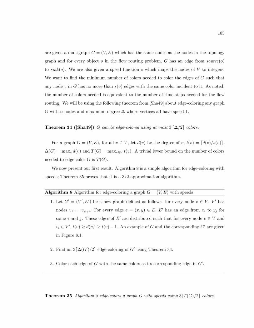
105
are given a multigraph G = (V, E) which has the same nodes as the nodes in the topology
graph and for every object o in the flow routing problem, G has an edge from source(o)
to sink(o). We are also given a speed function s which maps the nodes of V to integers.
We want to find the minimum number of colors needed to color the edges of G such that
any node v in G has no more than s(v) edges with the same color incident to it. As noted,
the number of colors needed is equivalent to the number of time steps needed for the flow
routing. We will be using the following theorem from [Sha49] about edge-coloring any graph
G with n nodes and maximum degree ∆ whose vertices all have speed 1.
Theorem 34 ([Sha49]) G can be edge-colored using at most 3 ∆/2 colors.
For a graph G = (V, E), for all v ∈ V , let d(v) be the degree of v, t(v) = d(v)/s(v),
∆(G) = maxv d(v) and T (G) = maxv∈V t(v). A trivial lower bound on the number of colors
needed to edge-color G is T (G).
We now present our first result. Algorithm 8 is a simple algorithm for edge-coloring with
speeds; Theorem 35 proves that it is a 3/2-approximation algorithm.
Algorithm 8 Algorithm for edge-coloring a graph G = (V, E) with speeds
1. Let G′ = (V ′, E′) be a new graph defined as follows: for every node v ∈ V , V ′ has
nodes v1, . . . vs(v). For every edge e = (x, y) ∈ E, E′ has an edge from xi to yj for
some i and j. These edges of E′ are distributed such that for every node v ∈ V and
vi ∈ V ′, t(v) ≥ d(vi) ≥ t(v)− 1. An example of G and the corresponding G′ are given
in Figure 8.1.
2. Find an 3∆(G′)/2 edge-coloring of G′ using Theorem 34.
3. Color each edge of G with the same colors as its corresponding edge in G′.
Theorem 35 Algorithm 8 edge-colors a graph G with speeds using 3T (G)/2 colors.
106
a1 b1 b2 b3
c1 c2 d1
b4
G’:
a b
c d
(1)
(2)
(4)
(1)
G:
Figure 8.1: The graph G is a demand graph with speeds given in parenthesis. The graphG′ is the graph constructed by Theorem 35
Proof: Consider the graph G′ created in the first step of the algorithm. We note that by
construction, ∆(G′) = T (G). Hence the coloring for G′ found in the second step of the
algorithm uses no more than 3T (G)/2 colors. Finally, the edge-coloring of G we get in
the third step of the algorithm uses 3T (G)/2 colors and has the property that no node v
has more that s(v) monochromatic edges incident to it.
8.2.1 Speeds that are Multiples of 2
In practice, for certain data migration applications, it is possible to directly increase the
speed of nodes by buying faster resources. For example, we can increase the speed of a
LAN in a disk farm by adding more disks to it. Results in this subsection are of use to
practitioners in that they give a principled way to build up resources in a network so as to
minimize migration time.
Corollary 37 shows that we can get very good results for edge-coloring with speeds if
the speeds are all multiples of 2. The basic idea behind the Corollary is to create a bipar-
tite graph by splitting the nodes and distributing the edges appropriately. The Corollary
depends on Lemma 36.
Lemma 36 There is a polytime algorithm to get an edge coloring using T (G) colors for
any graph G = (V, E) which has all node even degree and for which for all nodes v ∈ V ,

107
s(v) is even.
Proof: We first create a new graph G′ = (V ′, E′) which for every node v ∈ V , contains the
nodes v′1, . . . , v′s(v). To determine the edges G′, we first give each edge of G an orientation by
taking an Eulerian tour on G treated as an undirected graph. For an edge e = (x, y) ∈ E,
we say e is oriented from x to y if when e is traversed in the tour x is visited before y.
Otherwise we say that e is oriented from y to x.
For each edge in G oriented from node x to node y, we have edge (x′i, y
′j) where i is
some odd number between 1 and s(x) and j is some even number between 1 and s(y). We
distribute the edges such that ∀v ∈ V and ∀i1 ≤ i ≤ s(v), d(vi) ≤ t(vi).
G′ is now a bipartite graph where the left side is all nodes of form v′i for any v where i
is odd and the right side is all nodes of form v′j for any v where j is even. There is also a
1 − 1 mapping between the edges of G and the edges of G′ and ∆(G′) = T (G)
Since G′ is bipartite, it is well known that we can color it with ∆(G′) colors. Such a
coloring gives an edge coloring with speeds of G which uses T (G) colors.
Corollary 37 If all speeds are multiples of 2, we can edge color with speeds in 2T (G)/2
with no bypass nodes.
Proof: We can add dummy edges to G to ensure that all nodes have even degree while
increasing the maximum degree to at most 2 T (G)/2 (the procedure for doing this is trivial
and was given in Section 6.3.1). We then edge color this new graph using the algorithm in
Lemma 36.
8.3 Migration on Trees
In this section, we present results on the problem of migration on trees. This is simply the
flow routing problem on trees when there are no space constraints. Since on trees there is
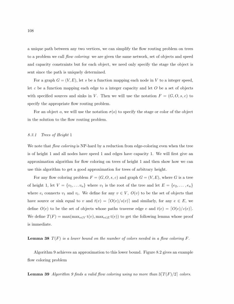
108
a unique path between any two vertices, we can simplify the flow routing problem on trees
to a problem we call flow coloring: we are given the same network, set of objects and speed
and capacity constraints but for each object, we need only specify the stage the object is
sent since the path is uniquely determined.
For a graph G = (V, E), let s be a function mapping each node in V to a integer speed,
let c be a function mapping each edge to a integer capacity and let O be a set of objects
with specified sources and sinks in V . Then we will use the notation F = (G, O, s, c) to
specify the appropriate flow routing problem.
For an object o, we will use the notation σ(o) to specify the stage or color of the object
in the solution to the flow routing problem.
8.3.1 Trees of Height 1
We note that flow coloring is NP-hard by a reduction from edge-coloring even when the tree
is of height 1 and all nodes have speed 1 and edges have capacity 1. We will first give an
approximation algorithm for flow coloring on trees of height 1 and then show how we can
use this algorithm to get a good approximation for trees of arbitrary height.
For any flow coloring problem F = (G, O, s, c) and graph G = (V, E), where G is a tree
of height 1, let V = v1, . . . vn where v1 is the root of the tree and let E = e2, . . . , en
where ei connects v1 and vi. We define for any v ∈ V , O(v) to be the set of objects that
have source or sink equal to v and t(v) = O(v)/s(v) and similarly, for any e ∈ E, we
define O(e) to be the set of objects whose paths traverse edge e and t(e) = O(e)/c(e).
We define T (F ) = max(maxv∈V t(v), maxe∈E t(e)) to get the following lemma whose proof
is immediate.
Lemma 38 T (F ) is a lower bound on the number of colors needed in a flow coloring F .
Algorithm 9 achieves an approximation to this lower bound. Figure 8.2 gives an example
flow coloring problem
Lemma 39 Algorithm 9 finds a valid flow coloring using no more than 3T (F )/2 colors.
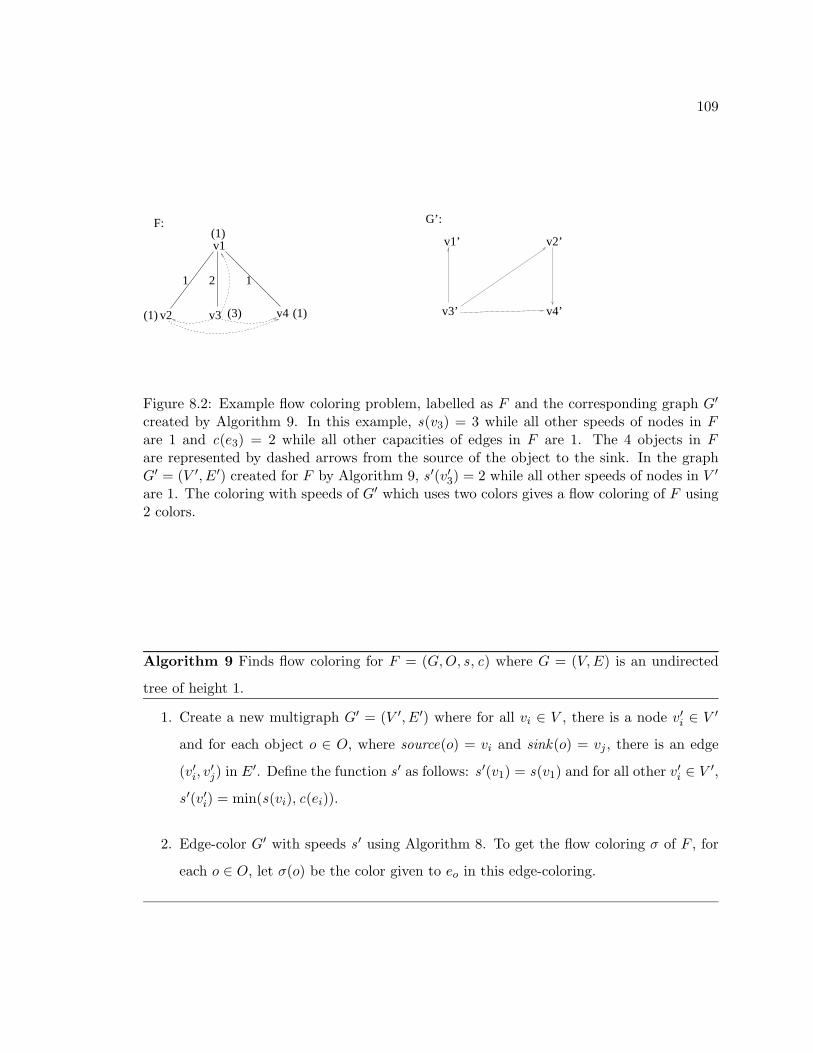
109
v1’ v2’
v3’ v4’
G’:F:
v2 v3 v4
v1
(1)
1
(1) (3)
(1)
2 1
Figure 8.2: Example flow coloring problem, labelled as F and the corresponding graph G′
created by Algorithm 9. In this example, s(v3) = 3 while all other speeds of nodes in Fare 1 and c(e3) = 2 while all other capacities of edges in F are 1. The 4 objects in Fare represented by dashed arrows from the source of the object to the sink. In the graphG′ = (V ′, E′) created for F by Algorithm 9, s ′(v′3) = 2 while all other speeds of nodes in V ′
are 1. The coloring with speeds of G′ which uses two colors gives a flow coloring of F using2 colors.
Algorithm 9 Finds flow coloring for F = (G, O, s, c) where G = (V, E) is an undirected
tree of height 1.
1. Create a new multigraph G′ = (V ′, E′) where for all vi ∈ V , there is a node v′i ∈ V ′
and for each object o ∈ O, where source(o) = vi and sink(o) = vj , there is an edge
(v′i, v′j) in E′. Define the function s ′ as follows: s ′(v1) = s(v1) and for all other v′i ∈ V ′,
s ′(v′i) = min(s(vi), c(ei)).
2. Edge-color G′ with speeds s ′ using Algorithm 8. To get the flow coloring σ of F , for
each o ∈ O, let σ(o) be the color given to eo in this edge-coloring.
110
Proof: We note that T (G′) ≤ T (F ) so the edge-coloring of G uses no more than 3 T (F )/2
colors by Theorem 35. We next show that for any edge-coloring of G′, if we assign the color
given to each edge in E′ to its corresponding object in O then we get a valid flow coloring of
F . To see this, consider any edge ei ∈ E and the corresponding node v′i ∈ V ′. For any color
t, v′i has no more than min(s(vi), c(ei)) edges of color t incident to it in the edge-coloring of
G′. Hence for any color t, there are no more than c(ei) objects that traverse edge ei that
are colored t in the flow coloring of F . For similar reasons, for any color t and node vi ∈ V ,
there are no more than s(vi) objects with source or sink equal to vi that are colored t in
the flow coloring of F .
8.3.2 Trees of Arbitrary Height
In the algorithm for trees of arbitrary heights, we need the notion of a restriction of a set
of objects. For flow coloring problem F = (G, O, s, c) where G = (V, E) a tree, and for any
V ′ ⊂ V , the restriction of O to V ′ is a new set of objects O′ where for each o ∈ O whose
path P from source to sink in G crosses a node in V ′, there is a o′ ∈ O′ which has source
equal to the first node in P in V ′ and sink equal to the last node in P in V ′.
Now assume we have a flow problem F = (G, O, s, c) where G is a tree with root v1
which has child nodes v2, . . . , vl. We define Sub(F, vi) = (Gi, Oi, s ′, c′) to be a flow coloring
problem where Gi is the subtree rooted at vi with v1 added as another child of vi and Oi
the set of objects O restricted to Gi. All speeds and edge capacities are the same in the new
problem except that node v1 has speed |O(vi)|. We define Local(F, v1) = (G′, O′, s ′, c) to be
a flow coloring problem where G′ is the height 1 tree consisting of v1 and all its children and
O′ is O restricted to the vertices in G′. All capacities are the same in this new problem as
is the speed of node v1. However ∀i 2 ≤ i ≤ l, s ′(vi) = |O(vi)|. Figure 8.3 gives examples
of Sub and Local problems. Algorithm 10 is the promised 3/2-approximation algorithm for
trees of arbitrary height.
For notational convenience in the proof of the approximation ratio for Algorithm 10, we
will, for a flow coloring F = (G, O, s, c), G = (V, E), let s(v, F ) be the speed in F of a

111
F:
v2
v4 v5
v8
v3
v1
v6 v7
Local(F,v1): v1’
v2’ v3’
Sub(F,v2): v2’
v4’ v5’ v1’
v8’o1
o2
o3
o3
o2
o1o3
o2
Figure 8.3: A flow coloring problem F and Local(F, v1) and Sub(F, v2) (dashed arrowsrepresent objects)
Algorithm 10 Finds flow coloring for F = (G, O, s, c) where G is a tree.
1. If G is of height 1, use Algorithm 9 to color F .
2. Let v1 be the root of G and let v2, . . . vl be the children of v1. Recursively color
Local(F, v1) and for all i = 2, . . . l, recursively color Sub(F, vi). Let σ1 be the coloring
of Local(F, v1) and σ2, . . . , σl be the colorings of Sub(F, v2), . . . ,Sub(F, vl).
3. For i = 2, . . . , l, permute the coloring σi such that for any o ∈ O that is in both
Local(F, v1) and Sub(F, vi) σi(o) is set to σ1(o) and such that two objects previously
assigned different colors in σi are still assigned different colors in the permutation of
σi (doing this with no more colors than the maximum number of colors used in σ1
and σi is trivial).
4. Each object o ∈ O is now assigned the same color in any of the colorings σ1, . . . , σl
that it appears in. This color is the color assigned to o in our flow coloring for F .
112
node v ∈ V and c(e, F ) be the capacity in F of an edge e ∈ E. Further, we let O(v, F ) be
the number of objects at vertex v in F and t(v, F ) = |O(v, F )|/s(v, F ). Similarly for any
edge e, we let t(e, F ) = |O(e, F )|/c(e, F ).
Theorem 40 Algorithm 10 finds a valid flow coloring using no more than 3T (F )/2 col-
ors.
Proof: We prove this by induction on the height of the tree G. The base case is established
by Lemma 39. For trees of height more than 1, we first show that the algorithm finds a
valid flow coloring and then show that the flow coloring found uses no more than 3T (F )/2
colors.
To show that the coloring of F is a valid flow coloring, consider some arbitrary node
u ∈ V . If u = v1 then s(u, F ) = s(u,Local(F, v1)). Further there is a 1 − 1 correspon-
dence between O(u, F ) and O(u,Local(F, v1)). By the inductive hypothesis, the objects
in O(u,Local(F, v1)) contain no more than s(u, F ) monochromatic objects. Hence, there
are no more than s(u, F ) monochromatic objects in O(u, F ). If u = v1 then for some
2 ≤ i ≤ l, s(u, F ) = s(u,Sub(F, vi)) and there is a 1 − 1 correspondence between O(u, F )
and O(u,Sub(F, vi)) so by an argument similar to the above, there are no more than s(u, F )
monochromatic objects in O(u, F ).
Next consider some arbitrary edge e ∈ E. We note that for some i, 2 ≤ i ≤ l, c(e, F ) =
c(e,Sub(F, vi)) and that there is a 1−1 correspondence between O(e, F ) and O(e,Sub(F, vi))
so again there are no more than c(e, F ) monochromatic objects in O(e, F ).
Finally, we show that the flow coloring found by the algorithm uses no more than
3T (F )/2 colors. We first note that in the last step of the algorithm, if we let M be the
maximum number of colors needed in any of the colorings of the subproblems, the coloring
of F has exactly M colors. Hence, if we show that T (Local(F, v1)) ≤ T (F ) and that for all
i, 2 ≤ i ≤ l, T (Sub(F, vi)) ≤ T (F ) then by the inductive hypothesis, we can achieve our
bound. In the following, we assume T (F ) ≥ 1.
Consider some vertex u that is both in F and Local(F, v1). We know that if u ∈
v2, . . . , vl then t(u,Local(F, v1)) = 1 (since s(u,Local(F, v1)) = |O(u,Local(F, v1))|). We
113
also know that if u = v1, s(u, F ) = s(u,Local(F, v1)) and |O(u,Local(F, v1))| = |O(u, F )|
so t(u, F ) = t(u,Local(F, v1)). So in either case, we know T (F ) ≥ t(u,Local(F, v1))
We also know that if u is in both F and Sub(F, vi) for some i, that if u = v1, t(u,Sub(F, vi)) =
1. On the other hand, if u = v1, s(u, F ) = s(u,Sub(f, vi)) and |O(u,Sub(f, vi))| = |O(v, F )|
so t(u, F ) = t(u,Sub(F, vi)). In either case, T (F ) ≥ t(u,Sub(F, vi))
Next consider some edge e in the problem F . We know that c(e, F ) = c(e,Local(F, v1))
and c(e, F ) = c(e,Sub(F, vi)) for any i, 2 ≤ i ≤ l. We also know that if e is in Local(F, v1)
then |O(e,Local(F, v1))| = |O(e, F )| so t(e,Local(F, v1)) = t(e, F ). A similar argument
shows that if e appears in Sub(F, vi) for any i, 2 ≤ i ≤ l, that t(e,Sub(F, vi)) = t(e, F ).
Putting these bounds together show that T (Local(F, v1)) ≤ T (F ) and for all i, 1 ≤ i ≤ l,
T (Sub(F, vi)) ≤ T (F ).
We note that if speeds of all nodes and capacities of all edges are multiples of 2, that by
using Corollary 37, we can find a flow coloring for the tree which is essentially the optimal
number of stages.
8.4 Migration with Splitting
In this section, we will be considering the problem of migration with splitting. This is
simply the general flow routing problem on an arbitrary topology in the presence of space
constraints where splitting of data objects is allowed. We will give a (1 + ε)-approximation
algorithm for this problem when objects can be split into a fairly large number of pieces.
Let F = (G, O) be a flow routing problem over graph G = (V, E) with object set O.
Let the speeds and memory at nodes be given by functions s and m respectively and let
capacities at edges be given by the function c. For some integer α, we define F ′ = split(F, α)
to be a new flow routing problem over G defined as follows. Each node v in F ′ has speed
αs(v) and memory αm(v) while each edge e in F ′ has capacity αc(e). For each object
o ∈ O, F ′ contains α objects each with source source(o) and sink sink(o). Formally, if we
are given F , and we can find a flow routing for F ′, in k stages, then we say that if the
objects of F are split into α pieces, we can route F in k stages. Our reasoning behind this is

114
as follows: in one stage in the migration with pieces, a storage device multiplexes over the
object pieces that it is assigned to send or recieve (i.e. the stage is divided into time slices
and the device spends one time slice on each object). If a device v has speed s and memory
m, it can send or receive αs object pieces in one stage by multiplexing and can store αm
pieces at the end of each stage. Similarly, each edge with capacity c can handle αc object
pieces in one stage. We note that there will be an overhead due to the multiplexing so that
in practice, a stage of sending pieces of objects will take somewhat longer that a stage of
sending the objects.
8.4.1 Preliminaries
In our approximation algorithm, we will round a solution to a certain multicommodity flow
problem to get an integer multicommodity flow and then use this integer multicommodity
flow to create a valid flow routing. We depend on the following corollary to a result by
Raghavan and Thompson [RT87] whose proof is given here for completeness.
Corollary 41 Let δ be any fixed number such that 0 < δ <√
5−12 . Assume we are given a
fractional multicommodity flow over a graph G = (V, E) which sends exactly one unit of each
commodity and that the the amount of flow over every edge is no more than (1 − δ) times
the capacity of that edge and that each edge has capacity at least β. Then with probability
greater than 1 − 2|E|e−.38δ2β, we can find an integral multicommodity flow over G which
sends exactly one unit of each commodity.
Proof: For each commodity i, let si be the source node of i and ti be the sink node of i.
Further, for each commodity i and edge e, let f(i, e) be the fractional flow of i sent through
e.
Our approach will be for each commodity i to perform a random walk from si to ti
guided by the fractional flows f(i, e). The random walk for commodity i begins at si. Now
suppose we are at a node v in the walk and let A(v) be the set of edges leaving v. The
random walk chooses to proceed along edge a ∈ A(v) with probability f(i,a)∑e∈A(v)f(i,e)
. The
walk terminates at reaching ti which it must since we can assume with out loss of generality
that the set of edges with non-zero flow form a directed acyclic graph.
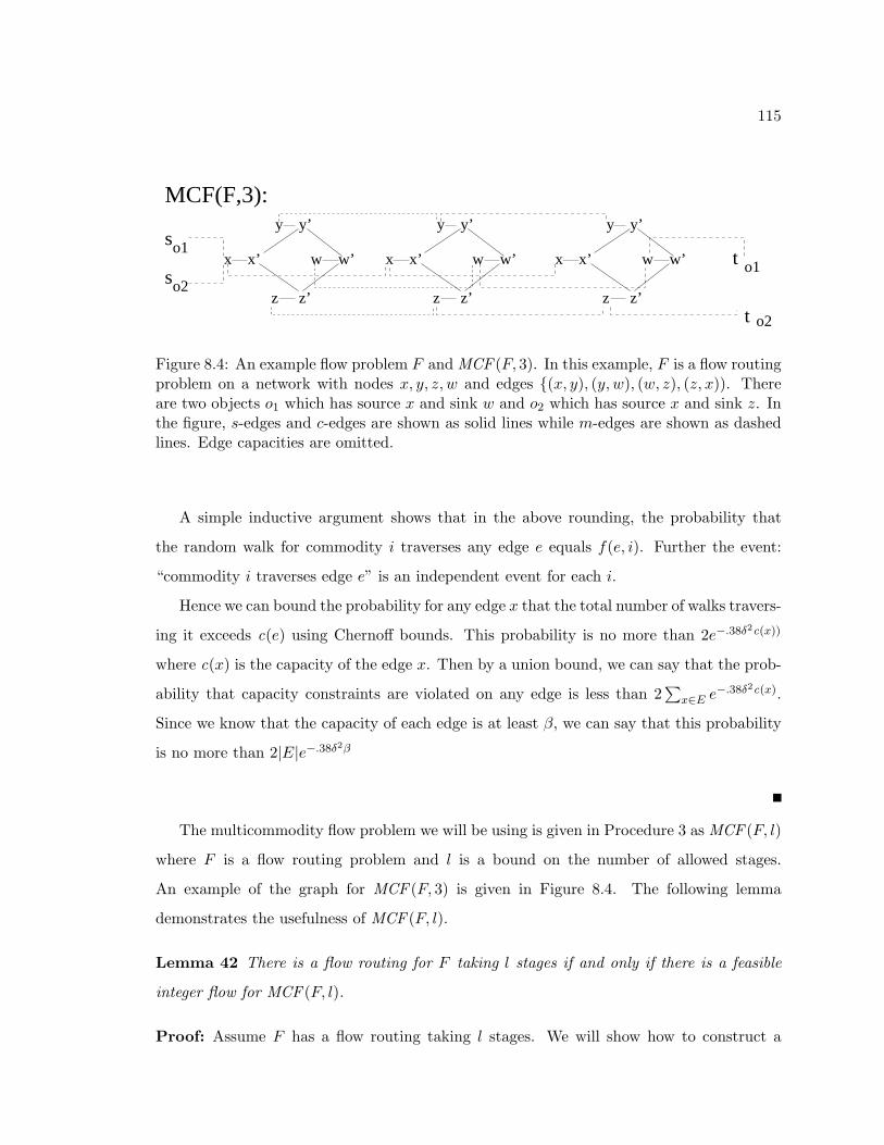
115
x x’
y y’
z z’
w w’ x x’
y y’
z z’
w w’ x x’
y y’
z z’
w w’so1
so2
MCF(F,3):
t o1
o2t
Figure 8.4: An example flow problem F and MCF (F, 3). In this example, F is a flow routingproblem on a network with nodes x, y, z, w and edges (x, y), (y, w), (w, z), (z, x)). Thereare two objects o1 which has source x and sink w and o2 which has source x and sink z. Inthe figure, s-edges and c-edges are shown as solid lines while m-edges are shown as dashedlines. Edge capacities are omitted.
A simple inductive argument shows that in the above rounding, the probability that
the random walk for commodity i traverses any edge e equals f(e, i). Further the event:
“commodity i traverses edge e” is an independent event for each i.
Hence we can bound the probability for any edge x that the total number of walks travers-
ing it exceeds c(e) using Chernoff bounds. This probability is no more than 2e−.38δ2c(x))
where c(x) is the capacity of the edge x. Then by a union bound, we can say that the prob-
ability that capacity constraints are violated on any edge is less than 2∑
x∈E e−.38δ2c(x).
Since we know that the capacity of each edge is at least β, we can say that this probability
is no more than 2|E|e−.38δ2β
The multicommodity flow problem we will be using is given in Procedure 3 as MCF (F, l)
where F is a flow routing problem and l is a bound on the number of allowed stages.
An example of the graph for MCF (F, 3) is given in Figure 8.4. The following lemma
demonstrates the usefulness of MCF (F, l).
Lemma 42 There is a flow routing for F taking l stages if and only if there is a feasible
integer flow for MCF (F, l).
Proof: Assume F has a flow routing taking l stages. We will show how to construct a

116
Procedure 3 Creates multicommodity flow problem MCF (F, l) for integer l and flow prob-
lem F = (G, O, s, c) where G = (V, E).
1. We first create a graph G′ from G = (V, E) on which to route the flow. For each
vertex v ∈ V , for each i = 1, . . . , l, G′ contains vertices vi and v′i. For each o ∈ O, G′
contains source node so and sink node to. Edges are created in the following way:
• For each edge e = (v, w) ∈ E and for each i = 1, . . . , l, G′ contains the edge
(v′i, w′i) with capacity c(e). We call such edges c-edges since they enforce capacity
constraints.
• For each node v ∈ V and for each i = 1, . . . , l, G′ contains the edge (vi, v′i) with
capacity s(v). We call such edges s-edges since they enforce speed constraints.
• For each node v ∈ V and for each i = 1, . . . , l− 1, G′ contains the edge (vi, vi+1)
with capacity m(v). For each o ∈ O, with source x and sink y, G′ also contains
the edge (so, x1) with capacity m(x) and edge (yl, to) with capacity m(y). We
call all such edges m-edges since they enforce memory constraints.
2. The flow problem is defined as follows: for each o ∈ O, we demand that one unit of
commodity o be routed from node so to node to in G′.

117
feasible integer multicommodity flow for MCF (F, l). Consider any object o ∈ O, which is
routed along some path P from a to b at stage i < l in the flow routing. We will send
commodity o through the following edges in MCF (F, l). First we will send it through edge
(ai, a′i) ,then for each edge (x, y) ∈ P , we send it through edge (x′
i, y′i) and finally we will
send it through the edges (b′i, bi) and (bi, bi+1). For each commodity o, with source v and
sink w, we will send commodity o through edge (so, v1) and through edge (vl, to).
The capacities of the s-edges, c-edges and m-edges in MCF (F, l) are not exceeded by our
assumption that the flow routing is valid. In particular, consider some s-edge, (vi, v′i), for
vertex v and stage i. We know that no more than s(v) objects begin or end at v in our flow
routing and so we know that no more than s(v) units of commodity traverse this edge. Now
consider some m-edge, (vi, vi+1), for some vertex v. We know that the number of objects
on the node of v at the end of any stage of the flow routing is no more than m(v) so we also
know that no more than m(v) units of commodity traverse this edge. Finally, consider some
c-edge, (v′i, w′i), for some nodes v and w and some stage i. Let e be the edge between v and
w in the topology graph. Then we know that no more than c(e) objects traverse edge e at
stage i in the flow routing so we know that no more that c(e) units of commodity traverse
edge (v′i, w′i). We also know that one unit flow of each commodity is sent in our constructed
flow since our assumed flow routing sends every object from its source to its sink.
Now assume there is a feasible integer multicommodity flow, f , for the problem MCF (F, l).
We construct a flow routing taking l stages as follows. For each object o, let (ai, a′i), P, (b′i, bi)
be a sequence of the edges in the path that commodity o is sent along where P is a sequence
of edges of the type (x′i, y
′i) for any vertices x and y. Then in stage i of the flow routing, we
send object o from vertex a to vertex b along edge path P . The speed, capacity and space
constraints in the flow routing are respected by arguments similar to those given above since
since f is a valid flow. In addition, our flow routing takes l stages by construction.

118
8.4.2 The Algorithm
We can now give the entire algorithm for computing a flow routing on an arbitrary topology;
the algorithm is given as Algorithm 11. Algorithm 11 uses Procedures 3 and 4. The proof
of its correctness uses lemmas 42 and 44.
Theorem 43 For a flow routing F = (G, O, s, c) which has a solution taking l∗ time steps,
Algorithm 11 gives a routing for any 0 < ε < 1 using no more than (1 + ε)l∗ time steps.
The algorithm splits the objects into α pieces where α is (1 + 1/ε)2/.38 ln(2ne) and ne =
(2|V | + |E|) (1 + ε)l∗)
Proof: The proof is immediate from Lemmas 42 and 44.
Algorithm 11 Given a flow routing problem F = (G, O, s, c) and a fixed constant 0 < ε < 1,
finds for a certain α, a flow routing for F taking no more than (1 + ε) times the optimal
number of time steps when the objects in O are split into α pieces.
1. Do binary search on l ∈ 1, . . . , |O| to find smallest l for which a feasible flow exists
for MCF (F, l). Let l∗ be the smallest such l and let f be the feasible flow for MCF (F, l∗)
2. Let F ′ = split(F ). We now use f to define a feasible flow f ′ for MCF (F ′, l∗) as follows.
Let fo(e) be the flow of commodity o through edge e in the flow f . For all i, 1 ≤ i ≤ α
set f ′oi
(e) = fo(e) where oi is the commodity associated with the i-th copy of object o
in F ′.
3. Round the flow f ′ using Procedure 4 to get an integral flow fi for MCF (F ′, (1+ ε)l∗).
4. Use fi and Lemma 42 to get a flow routing for F ′ using (1 + ε)l∗ stages.
Lemma 44 Procedure 4 finds with high probability a flow routing for F ′ = split(F, β) taking
(l + ε)1∗ stages.
119
Procedure 4 Let ε > 0, f be a flow for MCF (F ′, l) (where F ′ = split(F, β) and β is as in
Lemma 44). Finds an integral flow for MCF (F, (1 + ε)l) with high probability.
1. Let G = (V, E) be the graph we will find the flow over and δ = ε/(1 + ε). We create
f ′, a feasible fractional flow over MCF (F, (1 + ε)l) as follows. For each commodity
o, integer i, 1 ≤ i ≤ l and edge e = (x, y) ∈ E, let k = i/ε, ei = (xi, yi) be an
edge in MCF (F, l), e′i be the corresponding edge in MCF (F, (1 + ε)l) and e′l+k be the
edge (xk+l, yk+l) in MCF (F, (1 + ε)l). We set f ′(e′i, o) = (1 − δ)f(ei, o) and also set
f ′(e′l+k, o) = δf(ei, o).
2. Round the flow f ′ using the technique given in Corollary 41 to get a feasible integer
flow for MCF (F, (1 + ε)l) with high probability.
Proof: We show that the rounding in the first step of the procedure gives with high prob-
ability a feasible integer flow. First we note that for every edge e in MCF (F, (1 + ε)l),
f ′(e) ≤ (1− δ)c(e) where δ = ε/(1 + ε). This is immediate for edges in the level i subgraph
of MCF (F, (1 + ε)l) for i ≤ l and for all levels i > l, for any edge ei, there are at most
1/ε contributions of flow of size no more than (ε/(1 + ε))c(ei) to this edge so the total flow
is no more than (1/(1 + ε))c(ei) = (1 − δ)c(ei).
We will now apply Corollary 41 to get the desired result. We note that there are
ne = (|E| + 2|V |) (1 + ε)l edges total in MCF (F ′, (1 + ε)l) and each has capacity at
least β = ln 2ne/.38δ2. If we now apply Corollary 41 with δ as given above, we get that
the probability of success is bounded away from 0. Repeating the rounding in the first step
gives the desired high probability of success.

120
Chapter 9
CONCLUSION AND FUTURE WORK
9.1 Future Work
While this research has demonstrated the potential for designing provably good algorithms
for managing data in distributed systems, there are still many open problems. In this
section, we discuss open problems in the areas of peer-to-peer networking, data migration,
and embedded networks.
9.1.1 Peer-to-Peer Networks
Attack-Resistance
Many compelling empirical and theoretical problems remain open in the area of attack-
resistant peer-to-peer networks. Major empirical problems include:
• Can we create a usable real-world peer-to-peer system based on the deletion resistant
network and the control resistant network described in this thesis?
• For practical levels of attack-resistance, what will the constants be like in the resource
bounds for our attack-resistant networks? Are there heuristics which can, in practice,
significantly decrease these constants?
• What are the load balancing properties of our networks in practice?
Open theoretical problems include:
• For the deletion resistant network, is it possible to reduce the number of messages
that are sent in a search for a data item from O(log2 n) to O(log n)? For the control
121
resistant network, is it possible to reduce the number of messages sent in a search for
a data item from O(log3 n)?
• Can one deal efficiently with more general attacks? The control resistant network de-
scribed in this thesis is resistant to an adversary that makes nodes send fake messages,
but it is not resistant to an adversary that uses the nodes under its control to flood
the network and thereby shut it down. Can the ideas in this thesis be extended to
allow for resistance to this kind of attack?
• We conjecture that our networks have the property that they are poly-log competitive
with any fixed degree network. I.e., we conjecture that given any fixed degree network
topology, where n items are distributed amongst n nodes, and any set of access requests
that can be dealt with fixed sized buffers, then our network will also deal with the
same set of requests by introducing no more than a polylog slowdown. Can we prove
this result?
Restraining Free Riders
“Free Riders” are peers in a network which consume the resources of the network by doing
searches for content, but do not provide their own resources (e.g. storage space, bandwidth
and content) in return. In current peer-to-peer networks like Napster and Gnutella, a
significant fraction of the peers can currently be classified as free riders [SGG02, AH00].
The existence of these peers tends to degrade the performance and utility of the network.
One possible way to restrain the free rider problem is to try to enforce a set of rules
which will ensure “good” behavior for all the peers. An example rule might be something
like: “For every ten search request issued by a peer, that peer must service one search
request”. Given such a set of rules, the problem is how to enforce these rules for most of
the peers in the network even in the face of massive Byzantine faults.
Another, perhaps less draconian, approach to this problem is to assume that each peer
gets some benefit for receiving desired files from the network and pays some cost for pro-
viding resources to the network and then design a mechanism which ensures that there is
122
an economic incentive to provide resources. In particular, the network can then be modeled
as a coalitional game and the goal is to design a mechanism under which there is never an
economic incentive for some subset of peers to secede from the network.
Latency Aware Overlay Networks
A final compelling problem in peer-to-peer networks is designing algorithms for maintaining
peer-to-peer overlay topologies in such a way that peers which are close in the underlying In-
ternet are close in the overlay topology. Can we design an online algorithm which maintains
a topology such that most communication through the overlay occurs almost as efficiently
(say within a constant factor) as it would in the underlying Internet?
9.1.2 Data Migration
There are many open theory problems in the area of data migration. For the simplest prob-
lem of migration on the complete graph with homogeneous devices (the problem discussed
in Chapter 6), we have the following open questions:
• Is there a good approximation algorithm for migration with indirection when no ex-
ternal bypass nodes are available? In this thesis, we considered the problem of finding
near-optimal plans when a certain number of extra nodes are available as temporary
storage. While in many cases it is reasonable to assume there are extra nodes avail-
able, removing this assumption would make the formal results much more general. To
the best of our knowledge, no algorithm with an approximation ratio better than 3/2
for this problem is known at this time. 1
• What is the tradeoff between the number of bypass nodes available and the number
of stages (or colors) required? In this thesis, we established that if n/3 bypass nodes
are available that the number of stages is near optimal. What if we have somewhere
between 0 and n/3 bypass nodes? Can we get a good approximation guarantee, for
example, if we have n/6 bypass nodes?
1We note, however, that a recent result by Sanders and Solis-Oba [SSO00], gives a 6/5-approximationalgorithm for this problem when the data objects can be split into 5 pieces.

123
• What is the relationship between the chromatic index of a graph and its “chromatic
index with space constraints”? Are there better approximation algorithms for this
latter problem than those presented here? Is there a “Vizing-like” theorem for edge
coloring simple graphs with space constraints?
Another major area for future work in data migration is the online migration problem.
In this thesis, we have ignored loads imposed by user requests in devising a migration plan.
A better technique for creating a migration plan would be to migrate the objects in such
a way that we interfere as little as possible with the ability of the devices to satisfy user
requests and at the same time improve the load balancing behavior of the network as quickly
as possible. Since user requests are unpredictable, the loads imposed by data objects change
in an online manner over time. Can we design good online algorithms for this problem?
A final area for future work is exploring similarities between data migration and the
problem of routing in optical networks. While these two problems are in very different
application domains, their abstract formulations are similar. The results presented in this
thesis on data migration can likely be used as a basis for solving some important problems
in optical routing and conversely, some of the work in optical routing may be useful in
attacking open problems in data migration.
9.1.3 Embedded Networks
Embedded networks [CoNSoECTB01] are a burgeoning new area in distributed systems.
Audiovisual equipment, home and office appliances, automobiles, aircraft and buildings
already contain complex systems of embedded networked computers (EmNets), and the
number of application domains for embedded networks is growing rapidly. The opportunities
for good algorithm design in this area are extraordinary, as EmNets will be incorporated into
complex systems that people will depend on in unprecedented ways. EmNets will operate in
environments where resources such as power, time and bandwidth are severely constrained
and where robustness is extremely important.
It seems likely that some of the ideas in this thesis can be applied to problems in the area
of embedded networks. For example, fault tolerance is important in many EmNet systems

124
and as in peer-to-peer systems, each node in an EmNet is very vulnerable to attack but
there are massive numbers of nodes. In EmNets, we can actually build redundant nodes
into the system. An intriguing question is: Can we find a way to use redundant nodes
as efficiently as possible to ensure high degrees of attack-resistance for the EmNet? We
note that the definition of attack-resistance for EmNets would likely be different than the
definition of attack-resistance we have used for peer-to-peer networks.
Another compelling open problem is power-aware routing of data through EmNets. In
an EmNet, each node has some initial amount of power, and a node’s supply of power
decreases a fixed amount when transmitting a bit of information to another node. The
decrease in power for a communication is proportional to the physical distance between the
two nodes. In many applications, we would like to maximize the number of bits of data that
are routed through the network given these power constraints. This problem of power-aware
routing seems ripe for the same sort of algorithmic analysis that we have applied to the data
migration problem.
9.2 Conclusion
We now summarize the major contributions of this thesis.
9.2.1 Contributions
Contribution 1: A New Notion of Fault-Tolerance
In this thesis, we introduced a new notion of fault-tolerance which we call attack-
resistance. We define a network to be attack-resistant if it’s the case that after an adversary
deletes or controls a constant fraction of the nodes in the network an arbitrarily large frac-
tion of the remaining nodes can still access an arbitrarily large fraction of the content in
the network. This property of attack-resistance is simultaneously stronger and weaker than
common notions of fault-tolerance. The property is stronger in the sense that it holds true
even in the face of targetted attack of a constant fraction of the nodes in the network.
The property is weaker in the sense that it only guarantees that some large fraction of the
remaining nodes can access some large fraction of the remaining content. This is in contrast

125
to common notions of fault-tolerance in quorum systems [Gif79, MRW00, MRWW98] and
file storage systems [MWC00, AKK+00], where the guaranteed property is that even after
faults occur, each node can access each data item.
We note that our new notion of fault-tolerance is crucial for the domain of peer-to-
peer systems. The fact that the property holds true even when a constant fraction of the
peers in the network has been attacked is crucial since peers are particularly vulnerable to
attack. The weaker guarantee is crucial because without it, we would not be able to ensure
scalability. For example if we were to guarantee that every peer can access every data item
after attack, each peer would require an amount of storage which is linear in the number of
peers and data items. This kind of resource requirement is not scalable.
Contribution 2: Attack-Resistant Peer-to-peer Networks
We have designed two attack-resistant peer-to-peer networks. The deletion resistant
network is attack-resistant to an adversary which deletes up to an arbitrarily large constant
fraction of the peers. The control resistant network is resistant to an adversary which
controls some constant less than one half of the peers in the network. The networks are
attack-resistant in the sense that even after attack, an arbitrarily large constant fraction of
the remaining peers can access an arbitarily large constant fraction of the data items. We
have also designed a network which is robust in a highly dynamic environment: the network
is robust even if all of the old peers are repeatedly deleted provided that enough new peers
join.
Contribution 3: Definition of the Data Migration Problem
We have defined several intriguing and well-motivated twists on the traditional edge
coloring problem. These data migration problems are motivated by the real-world problem
of efficiently moving data through a network but are also mathematically rich and interesting
in their own right.
Contribution 4: Data Migration algorithms with good theoretical properties
We have introduced multiple provably good algorithms for the data migration problems.
Our main results are polynomial time algorithms for finding a near-optimal migration plan
in the presence of space constraints when a certain number of additional nodes is available
as temporary storage, and a 3/2-approximation for the case where data must be migrated
126
directly to its destination. These algorithms match the worst case bounds for this problem.
We have also introduced data migration algorithms for networks with different node and
link speeds and topologies which are not complete. In many cases, these algorithms also
match the theoretical worst case bounds.
Contribution 5: Data Migration algorithms with good empirical properties
We have empirically evaluated the performance of multiple data migration algorithms on
both random and real-world type data migration problems. The metrics we used to evaluate
the algorithms are: (1) the number of time steps required to perform the migration, and
(2) the number of bypass nodes used as intermediate storage devices. We have found
that several data migration algorithms with weaker theoretical bounds actually perform
better empirically. Not surprisingly, we have also found that for all the algorithms tested,
the theoretical bounds are overly pessimistic. We conclude that many of the algorithms
described in this thesis are both practical and effective for data migration.
9.2.2 Conclusion
In this thesis, we have addressed the problems of attack-resistance and data migration - two
problems of fundamental importance in the area of managing data in distributed systems.
We have defined multiple theoretical problems in these areas, described polynomial time
algorithms for solving these problems and proven that our algorithms have many desirable
properties. We have also shown that our algorithms for data migration have good empirical
properties.
127
BIBLIOGRAPHY
[AB96] Yonatan Aumann and Michael Bender. Fault tolerant data structures. In
IEEE Symposium on Foundations of Computer Science, 1996.
[AH00] E. Adar and B. Huberman. Free riding on gnutella, 2000.
[AHH+01] Eric Anderson, Joe Hall, Jason Hartline, Michael Hobbes, Anna Karlin,
Ram Swaminathan, and John Wilkes. An experimental study of data
migration algorithms t. In Workshop on Algorithm Engineering, 2001.
[AHK+01] E. Anderson, M. Hobbs, K. Keeton, S. Spence, M. Uysal, and A. Veitch.
Hippodrome: running circles around storage administration. Submitted
to Symposium on Operating System Principles, 2001.
[AKK+00] Noga Alon, Haim Kaplan, Michael Krivelevich, Dahlia Malkhi, and Julien
Stern. Scalable secure storage when half the system is faulty. In Proceed-
ings of the 27th International Colloquium on Automata, Languages and
Programming, 2000.
[And96] R. Anderson. The eternity service, 1996.
[AS00] Noga Alon and Joel Spencer. The Probabilistic Method, 2nd Edition. John
Wiley & Sons, 2000.
[BDET00] Bolosky, Douceur, Ely, and Theimer. Feasibility of a serverless distributed
file system deployed on an existing set of desktop pcs. In Proceedings of
the international conference on Measurement and modeling of computer
systems, pages 34–43, 2000.

128
[BGM+97] E. Borowsky, R. Golding, A. Merchant, L. Schreier, E.Shriver,
M.Spasojevic, and J. Wilkes. Using attribute-managed storage to achieve
QoS. In Presented at 5th Intl. Workshop on Quality of Service, Columbia
Univ., New York, June 1997.
[Bor00] John Borland. Gnutella girds against spam attacks. CNET News.com,
August 2000. http://news.cnet.com/news/0-1005-200-2489605.html.
[BR93] M. Bellare and P. Rogaway. Random oracles are practical: a paradigm for
designing efficient protocols. In The First ACM Conference on Computer
and Communications Security, pages 62–73, 1993.
[Cli] Clip2. Gnutella: To the bandwidth barrier and beyond.
http://dss.clip2.com/gnutella.html.
[CoNSoECTB01] Computer Science Committee on Networked Systems of Embedded Com-
puters and National Research Council Telecommunications Board. Em-
bedded, Everywhere: A Research Agenda for Networked Systems of Em-
bedded Computers. National Academy Press, 2001.
[Cou96] Transaction Processing Performance Council. TPC Benchmark D (Deci-
sion Support) Standard Specification Revision 2.1. Transaction Processing
Performance Council, 1996.
[Dav01] David Moore, Geoffrey Voelker and Stefan Savage. Inferring internet
denial-of-service activity. In Proceedings of the 2001 USENIX Security
Symposium, 2001.
[DR01] Peter Druschel and Antony Rowstron. PAST: A Large-Scale, Persistent
Peer-to-Peer Storage Utility. In Proceedings of the Eighth IEEE Work-
shop on Hot Topics in Operating Systems (HotOS-VIII), Schoss Elmau,
Germany, May 2001.
129
[ECL85] D.S. Johnson E.G. Coffman, M.R. Garey and A.S. Lapaugh. Scheduling
file transfers. In SIAM Journal on Computing, volume 14, pages 744–780,
1985.
[Fou] Electronic Freedom Foundation. Eff — censorship — internet censor-
ship legislation & regulation (cda, etc.) — archive. http://www.eff.org/-
pub/Censorship/Internet censorship bills.
[FS02] Amos Fiat and Jared Saia. Censorship Resistant Peer-To-Peer Content
Addressable Networks. In 13th annual ACM-SIAM Symposium on Dis-
crete Algorithms, 2002.
[GHKS98] M.D. Grammatikakis, D.F. Hsu, M. Kraetzl, and J. Sibeyn. Packet rout-
ing in fixed-connection networks: A survey. In Journal of Parallel and
Distributed Processing, volume 54, pages 77–132, 1998.
[Gif79] D.K. Gifford. Weighted voting for replicated data. In Proc. of the Seventh
ACM Symposium on Operating Systems Principles, pages 150–159, 1979.
[Gol84] M. K. Goldberg. Edge-coloring of multigraphs: Recoloring technique. J.
Graph Theory, 8:121–137, 1984.
[Gri02] Steve Gribble. private communication, 2002.
[GS90] B. Gavish and O. R. Liu Sheng. Dynamic file migration in distributed
computer systems. Communications of the ACM, 33:177–189, 1990.
[GSKTZ00] I. Golubchik, S. Khuller S. Khanna, R. Thurimella, and A. Zhu. Approx-
imation Algorithms for Data Placement on Parallel Disks. In Proceedings
of the Eleventh Annual ACM-SIAM Symposium on Discrete ALgorithms,
pages 223–232, 2000.
130
[GVY97] Naveen Garg, Vijay V. Vazirani, and Mihalis Yannakakis. Flow and mul-
ticut in trees. Algorithmica, 18(1):3–20, 1997.
[HHK+01] J. Hall, J. Hartline, A. Karlin, J. Saia, and J. Wilkes. On algorithms
for efficient data migration. In 12th annual ACM-SIAM Symposium on
Discrete Algorithms, 2001.
[Hia01] Brian Hiatt. With napster weakened, riaa hopes to settle land-
mark lawsuit, July 2001. http://www.mtv.com/sendme2.tin?page=/-
news/articles/1445466/20010727/index.jhtml.
[HLN89] J. Hastad, T. Leighton, and M. Newman. Fast computation using faulty
hypercubes. In Proceedings of the 21st Annual ACM Symposium on The-
ory of Computing, 1989.
[HNS96] D. S. Hochbaum, T. Nishizeki, and D. B. Shmoys. A better than “Best
Possible” algorithm to edge color multigraphs. J. of Algorithms, 7:79–104,
1996.
[Hoc95] Dorit Hochbaum, editor. Approximation Algorithms for NP-Hard Prob-
lems. PWS Publishing Company, 1995.
[Hoy81] I. J. Hoyer. The NP-completeness of edge coloring. SIAM J. Comput.,
10:718–720, 1981.
[KBC+00] John Kubiatowicz, David Bindel, Yan Chen, Steven Czerwinski, Patrick
Eaton, Dennis Geels, Ramakrishna Gummadi, Sean Rhea, Hakim Weath-
erspoon, Westley Weimer, Chris Wells, and Ben Zhao. Oceanstore: An
architecture for global-scale persistent storage. In Appears in Proceed-
ings of the Ninth international Conference on Architectural Support for
Programming Languages and Operating Systems (ASPLOS 2000), 2000.
131
[KNT94] Anna R. Karlin, Greg Nelson, and Hisao Tamaki. On the fault tolerance
of the butterfly. In ACM Symposium on Theory of Computing, 1994.
[Kub96] M. Kubale. ”Preemptive versus nonpreemptive scheduling of biproces-
sor tasks on dedicated processors”. In European Journal of Operational
Research, volume 94, pages 242–251, 1996.
[LMS98] Thomson Leighton, Bruce Maggs, and Ramesh Sitamaran. On the fault
tolerance of some popular bounded-degree networks. SIAM Journal on
Computing, 1998.
[LSP82] L. Lamport, R.E. Shostack, and M. Pease. The byzantine generals prob-
lem. In ACM Trans. Prog. Lang. and Systems, 1982.
[Mar] Robert Marquand. China’s web users kept on their toes.
http://www.csmonitor.com/durable/2000/12/07/fp7s1-csm.shtml.
[MR95] Rajeev Motwani and Prabhakar Raghavan. Randomized Algorithms.
Cambridge University Press, 1995.
[MRW00] Dahlia Malkhi, Michael Reiter, and Avishai Wool. The load and avail-
ability of byzantine quorum systems. SIAM Journal of Computing,
29(6):1889–1906, 2000.
[MRWW98] Dahlia Malkhi, Michael Reiter, Avishai Wool, and Rebecca N. Wright.
Probabilistic byzantine quorum systems. In Symposium on Principles of
Distributed Computing, 1998.
[MV80] Micali and Vazirani. An O(√
|V ||E|) algorithm for finding a maximum
matching in general graphs. In 21st Annual Symposium on Foundations
of Computer Science, 1980.

132
[MWC00] Aviel D. Rubin Marc Waldman and Lorrie Faith Cranor. Publius: A
robust, tamper-evident, censorship-resistant, web publishing system. In
Proc. 9th USENIX Security Symposium, pages 59–72, August 2000.
[Nar02] Narayanan. private communication, 2002.
[NK90] T. Nishizeki and K. Kashiwagi. On the 1.1 edge-coloring of multigraphs.
In SIAM Journal on Discrete Mathematics, volume 3, pages 391–410,
1990.
[NZN96] S. Nakano, X. Zhou, and T. Nishizeki. Edge Coloring Algorithms. In
Computer Science Today, pages 172–183, 1996.
[oC] Index on Censorship. Index on censorship homepage.
http://www.indexoncensorship.org.
[Ora01] Andy Oram, editor. Peer-to-Peer: Harnessing the Power of Disruptive
Technologies. O’Reilly & Associates, July 2001.
[Pin73] M. Pinsker. On the complexity of a concentrator. In 7th International
Teletraffic Conference, 1973.
[PRR97] C. Plaxton, R. Rajaram, and A.W. Richa. Accessing nearby copies of
replicated objects in a distributed environment. In Proceedings of the
Ninth Annual ACM Symposium on Parallel Algorithms and Architectures
(SPAA), 1997.
[PRU01] Gopal Pandurangan, Prabhakar Raghavan, and Eli Upfal. Building low-
diameter p2p networks. In STOC 2001, Crete, Greece, 2001.
[PST+97] Karin Petersen, Mike J. Spreitzer, Douglas B. Terry, Marvin M. Theimer,
and Alan J. Demers. Flexible update propagation for weakly consistent

133
replication. In Sixteen ACM Symposium on Operating Systems Principles,
1997.
[RFH+01] Sylvia Ratnasamy, Paul Francis, Mark Handley, Richard Karp, and Scott
Shenker. A Scalable Content-Addressable Network. In Proceedings of
the ACM SIGCOMM 2001 Technical Conference, San Diego, CA, USA,
August 2001.
[RT87] P. Raghavan and C. Thompson. Randomized Rounding. In Combinator-
ica, volume 7, pages 365–374, 1987.
[Sai] Yasushi Saito. Consistency management in optimistic replication algo-
rithms.
[SFG+02] Jared Saia, Amos Fiat, Steve Gribble, Anna R. Karlin, and Stefan Saroiu.
Dynamically fault-tolerant content addressable networks. In First Inter-
national Workshop on Peer-to-Peer Systems, 2002.
[SGG02] Stefan Saroiu, P. Krishna Gummadi, and Steven D. Gribble. A Mea-
surement Study of Peer-to-Peer File Sharing Systems. In Proceedings of
Multimedia Computing and Networking, 2002.
[Sha49] C. E. Shannon. A theorem on colouring lines of a network. J. Math.
Phys., 28:148–151, 1949.
[Sha79] Adi Shamir. How to share a secret. Communications of the ACM, 22,pp.
612–613, 1979.
[SMK+01] Ion Stoica, Robert Morris, David Karger, Frans Kaashoek, and Hari Bal-
akrishnan. Chord: A Scalable Peer-to-peer Lookup Service for Internet
Applications. In Proceedings of the ACM SIGCOMM 2001 Technical Con-
ference, San Diego, CA, USA, August 2001.

134
[SSO00] P. Sanders and R. Solis-Oba. How Helpers Hasten h-Relations. In Euro-
pean Symposium on Algorithms, 2000.
[Vaz01] Vijay Vazirani. Approximation Algorithms. Springer Verlag, 2001. pp73-
78.
[Viz64] V. G. Vizing. On an estimate of the chromatic class of a p-graph. Diskret.
Anal., 3:25–30, 1964.
[weba] Gnutella website. http://gnutella.wego.com/.
[webb] Napster website. http://www.napster.com/.
[Wol89] J. Wolf. The Placement Optimization Problem: a practical solution to
the disk file assignment problem. In Proceedings of the ACM SIGMET-
RICS international conference on Measurement and modeling of computer
systems, pages 1–10, 1989.
[ZKJ01] B.Y. Zhao, K.D. Kubiatowicz, and A.D. Joseph. Tapestry: An Infras-
tructure for Fault-Resilient Wide-Area Location and Routing. Technical
Report UCB//CSD-01-1141, University of California at Berkeley Techni-
cal Report, April 2001.
135
VITA
Jared Saia holds a B.S. degree from Stanford University and an M.S. degree from the
University of New Mexico. He has previously been a researcher at ATR Labs in Nara,
Japan. His primary technical interest is in designing and analyzing algorithms for practical
problems in computer systems and other application areas.