Embed Size (px)
Citation preview
Gunter Rote, Freie Universitat Berlin Algorithms for Isotonic Regression Graduiertenkolleg MDS, Berlin, 4. 2. 2013
Algorithms for Isotonic RegressionGunter Rote
Freie Universitat Berlinai
i
Gunter Rote, Freie Universitat Berlin Algorithms for Isotonic Regression Graduiertenkolleg MDS, Berlin, 4. 2. 2013
Algorithms for Isotonic RegressionGunter Rote
Freie Universitat Berlin
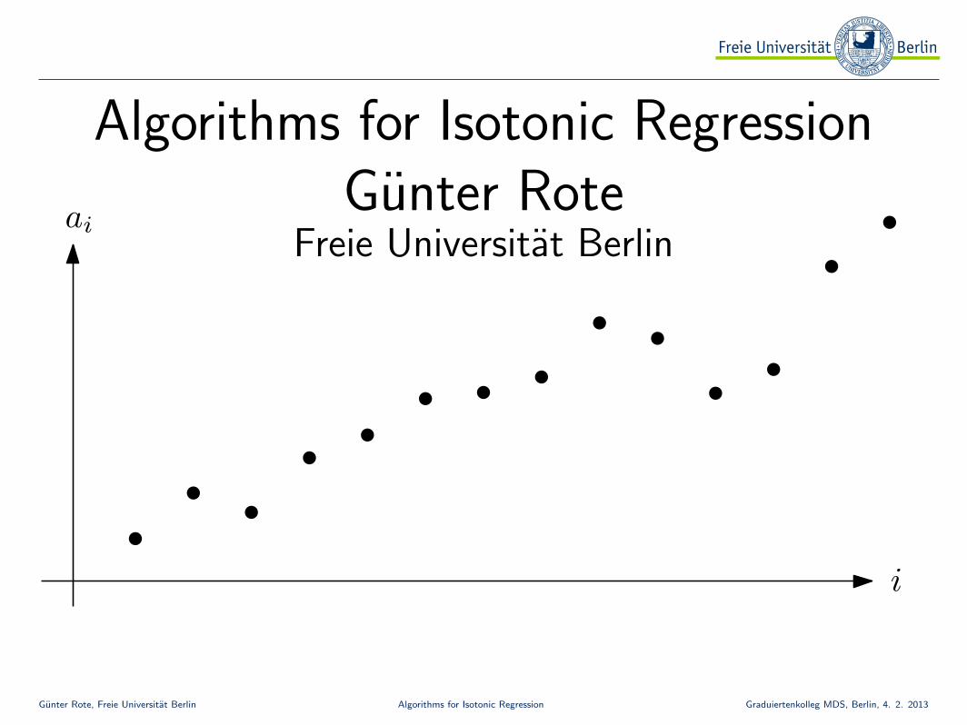
Minimizen∑
i=1
h(|xi − ai|) subject to x1 ≤ · · · ≤ xn
ai
i
|xi
Gunter Rote, Freie Universitat Berlin Algorithms for Isotonic Regression Graduiertenkolleg MDS, Berlin, 4. 2. 2013
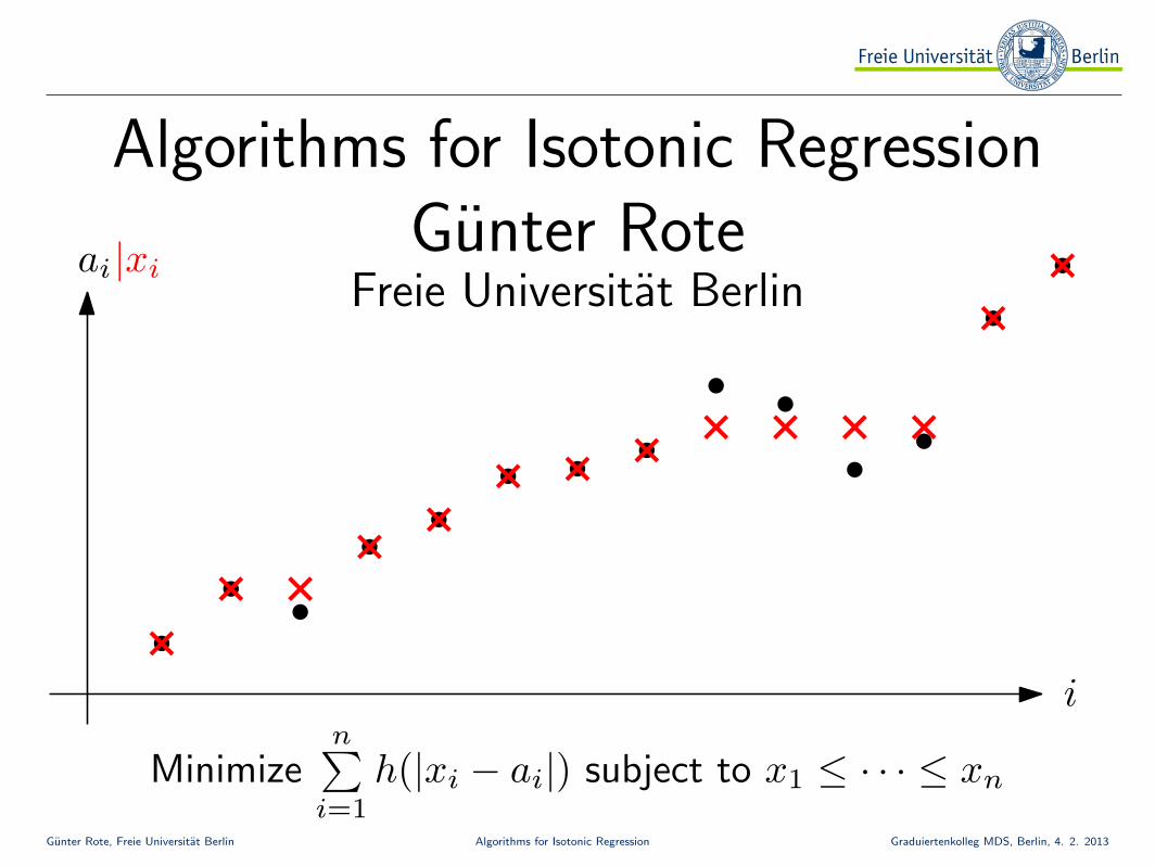
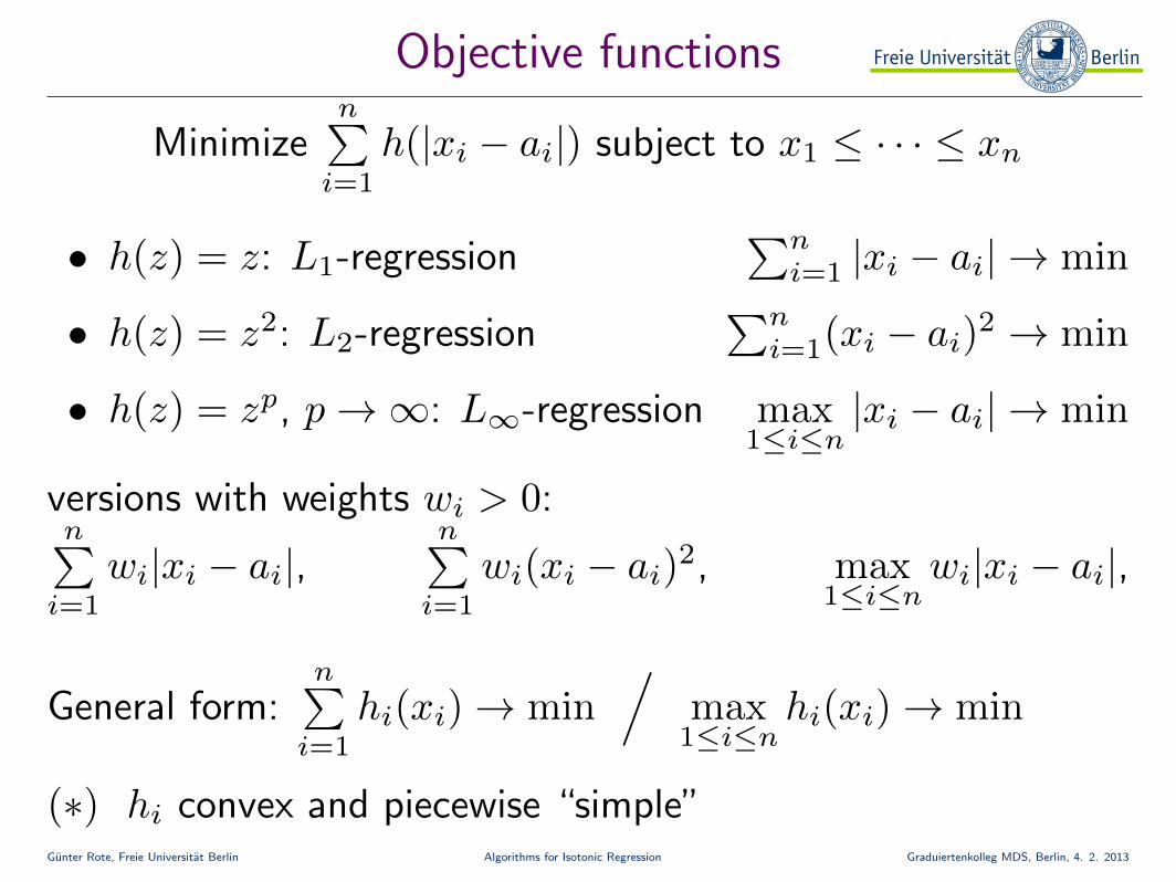
Objective functions
Minimizen∑
i=1
h(|xi − ai|) subject to x1 ≤ · · · ≤ xn
• h(z) = z: L1-regression∑n
i=1 |xi − ai| → min
• h(z) = z2: L2-regression∑n
i=1(xi − ai)2 → min
• h(z) = zp, p→∞: L∞-regression max1≤i≤n
|xi − ai| → min
versions with weights wi > 0:n∑
i=1
wi|xi − ai|,n∑
i=1
wi(xi − ai)2, max
1≤i≤nwi|xi − ai|,
General form:n∑
i=1
hi(xi)→ min/
max1≤i≤n
hi(xi)→ min
(∗) hi convex and piecewise “simple”
Gunter Rote, Freie Universitat Berlin Algorithms for Isotonic Regression Graduiertenkolleg MDS, Berlin, 4. 2. 2013
Overview
• The classical Pool Adjacent Violators (PAV) algorithm
• dynamic programming
• More general constraints:
xi ≤ xj for i ≺ j
with a given partial order ≺– In particular, Lmax regression with a d-dimensional
partial order– Randomized optimization technique of Timothy Chan
(1998)
Gunter Rote, Freie Universitat Berlin Algorithms for Isotonic Regression Graduiertenkolleg MDS, Berlin, 4. 2. 2013
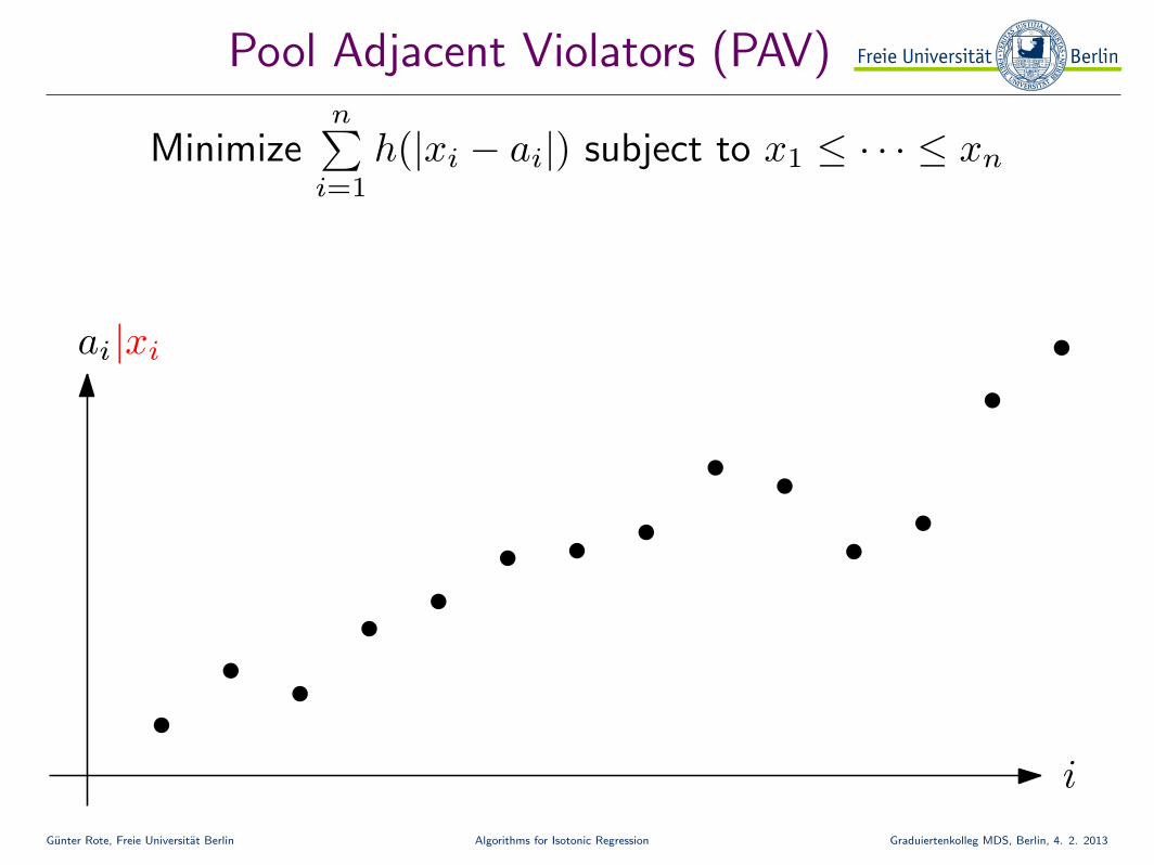
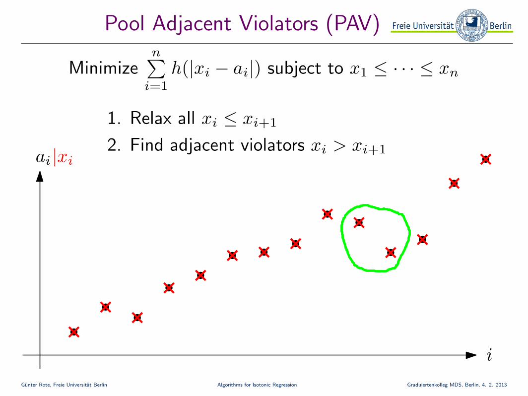
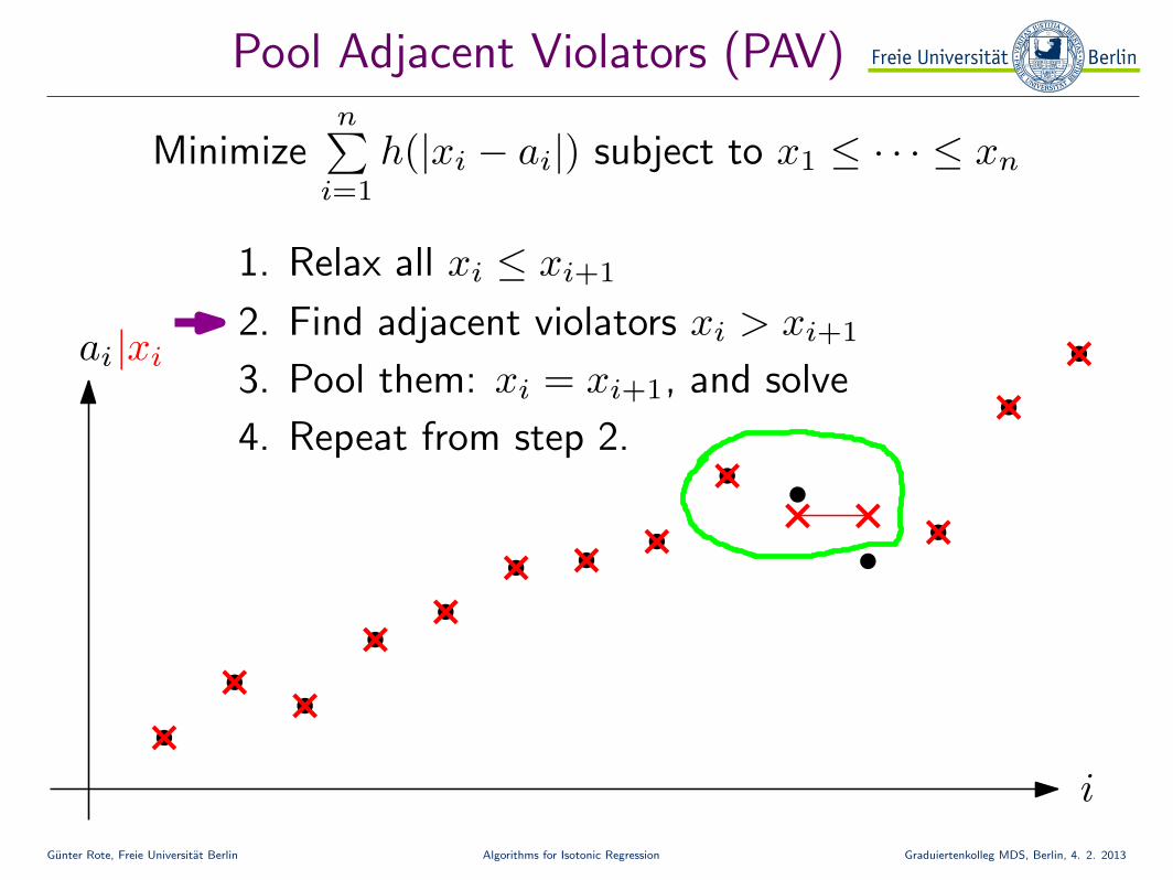
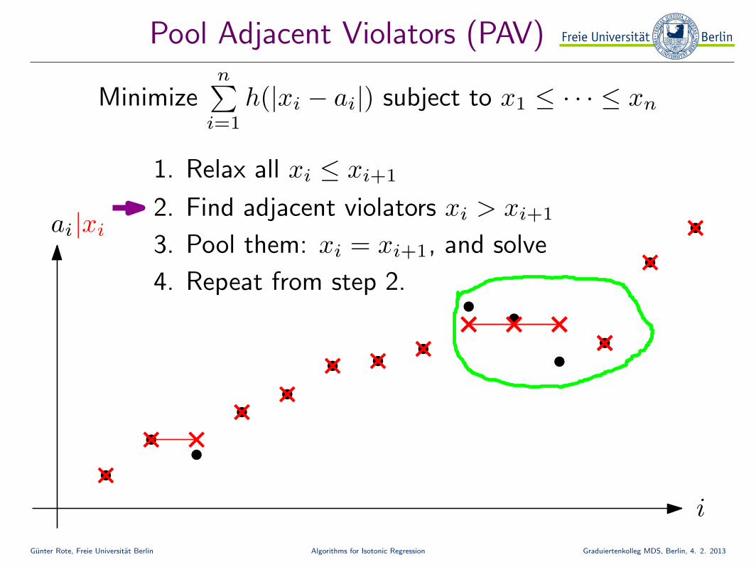
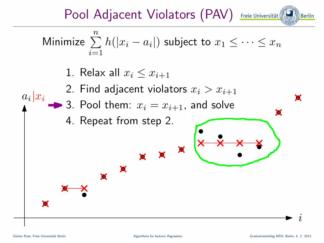
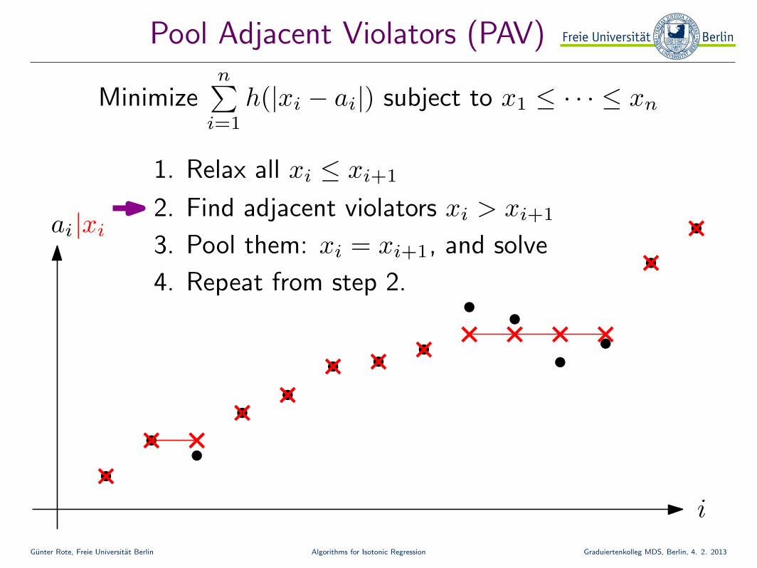
Pool Adjacent Violators (PAV)
Minimizen∑
i=1
h(|xi − ai|) subject to x1 ≤ · · · ≤ xn
ai
i
|xi
Gunter Rote, Freie Universitat Berlin Algorithms for Isotonic Regression Graduiertenkolleg MDS, Berlin, 4. 2. 2013
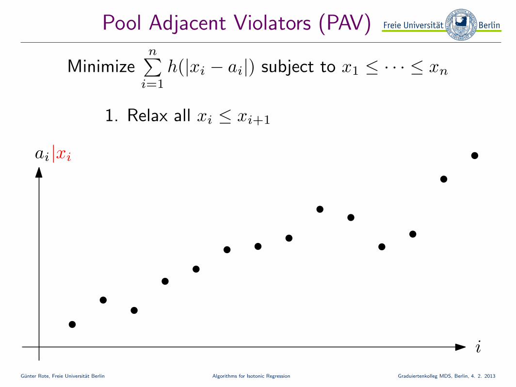
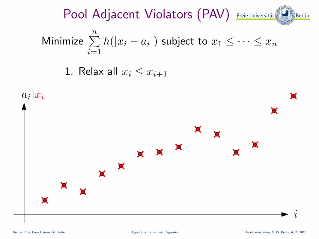
Pool Adjacent Violators (PAV)
Minimizen∑
i=1
h(|xi − ai|) subject to x1 ≤ · · · ≤ xn
ai
i
|xi
1. Relax all xi ≤ xi+1
Gunter Rote, Freie Universitat Berlin Algorithms for Isotonic Regression Graduiertenkolleg MDS, Berlin, 4. 2. 2013
Pool Adjacent Violators (PAV)
Minimizen∑
i=1
h(|xi − ai|) subject to x1 ≤ · · · ≤ xn
ai
i
|xi
1. Relax all xi ≤ xi+1
Gunter Rote, Freie Universitat Berlin Algorithms for Isotonic Regression Graduiertenkolleg MDS, Berlin, 4. 2. 2013
Pool Adjacent Violators (PAV)
Minimizen∑
i=1
h(|xi − ai|) subject to x1 ≤ · · · ≤ xn
ai
i
|xi
1. Relax all xi ≤ xi+1
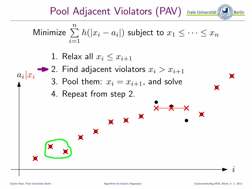
2. Find adjacent violators xi > xi+1
Gunter Rote, Freie Universitat Berlin Algorithms for Isotonic Regression Graduiertenkolleg MDS, Berlin, 4. 2. 2013
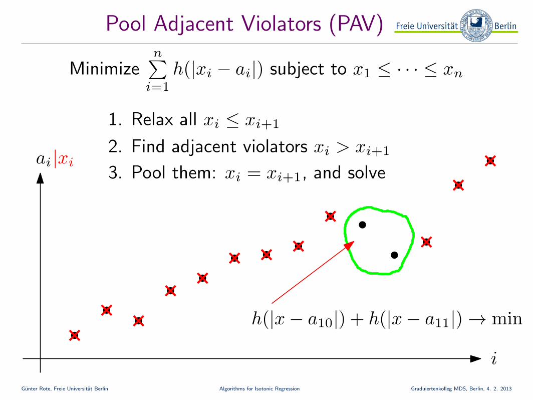
Pool Adjacent Violators (PAV)
Minimizen∑
i=1
h(|xi − ai|) subject to x1 ≤ · · · ≤ xn
ai
i
|xi
1. Relax all xi ≤ xi+1
2. Find adjacent violators xi > xi+1
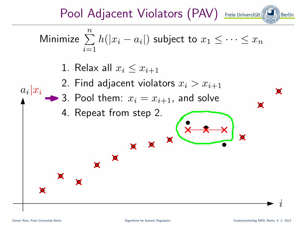
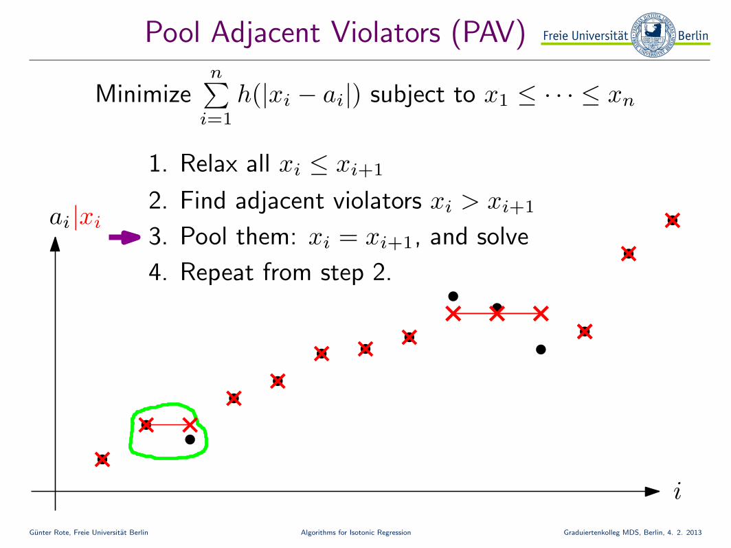
3. Pool them: xi = xi+1, and solve
h(|x− a10|) + h(|x− a11|)→ min
Gunter Rote, Freie Universitat Berlin Algorithms for Isotonic Regression Graduiertenkolleg MDS, Berlin, 4. 2. 2013
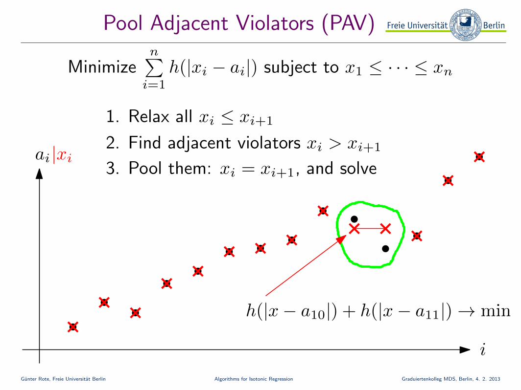
Pool Adjacent Violators (PAV)
Minimizen∑
i=1
h(|xi − ai|) subject to x1 ≤ · · · ≤ xn
ai
i
|xi
1. Relax all xi ≤ xi+1
2. Find adjacent violators xi > xi+1
3. Pool them: xi = xi+1, and solve
h(|x− a10|) + h(|x− a11|)→ min
Gunter Rote, Freie Universitat Berlin Algorithms for Isotonic Regression Graduiertenkolleg MDS, Berlin, 4. 2. 2013
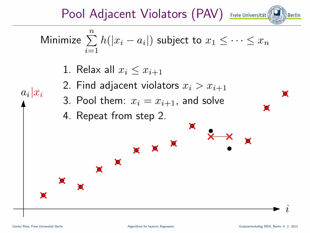
Pool Adjacent Violators (PAV)
Minimizen∑
i=1
h(|xi − ai|) subject to x1 ≤ · · · ≤ xn
ai
i
|xi
1. Relax all xi ≤ xi+1
2. Find adjacent violators xi > xi+1
3. Pool them: xi = xi+1, and solve
4. Repeat from step 2.
Gunter Rote, Freie Universitat Berlin Algorithms for Isotonic Regression Graduiertenkolleg MDS, Berlin, 4. 2. 2013
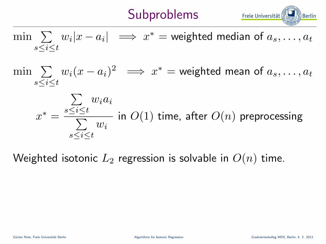
Subproblems
min∑
s≤i≤twi|x− ai| =⇒ x∗ = weighted median of as, . . . , at
min∑
s≤i≤twi(x− ai)
2 =⇒ x∗ = weighted mean of as, . . . , at
x∗ =
∑s≤i≤t
wiai∑s≤i≤t
wiin O(1) time, after O(n) preprocessing
Weighted isotonic L2 regression is solvable in O(n) time.
Gunter Rote, Freie Universitat Berlin Algorithms for Isotonic Regression Graduiertenkolleg MDS, Berlin, 4. 2. 2013
Subproblems
min∑
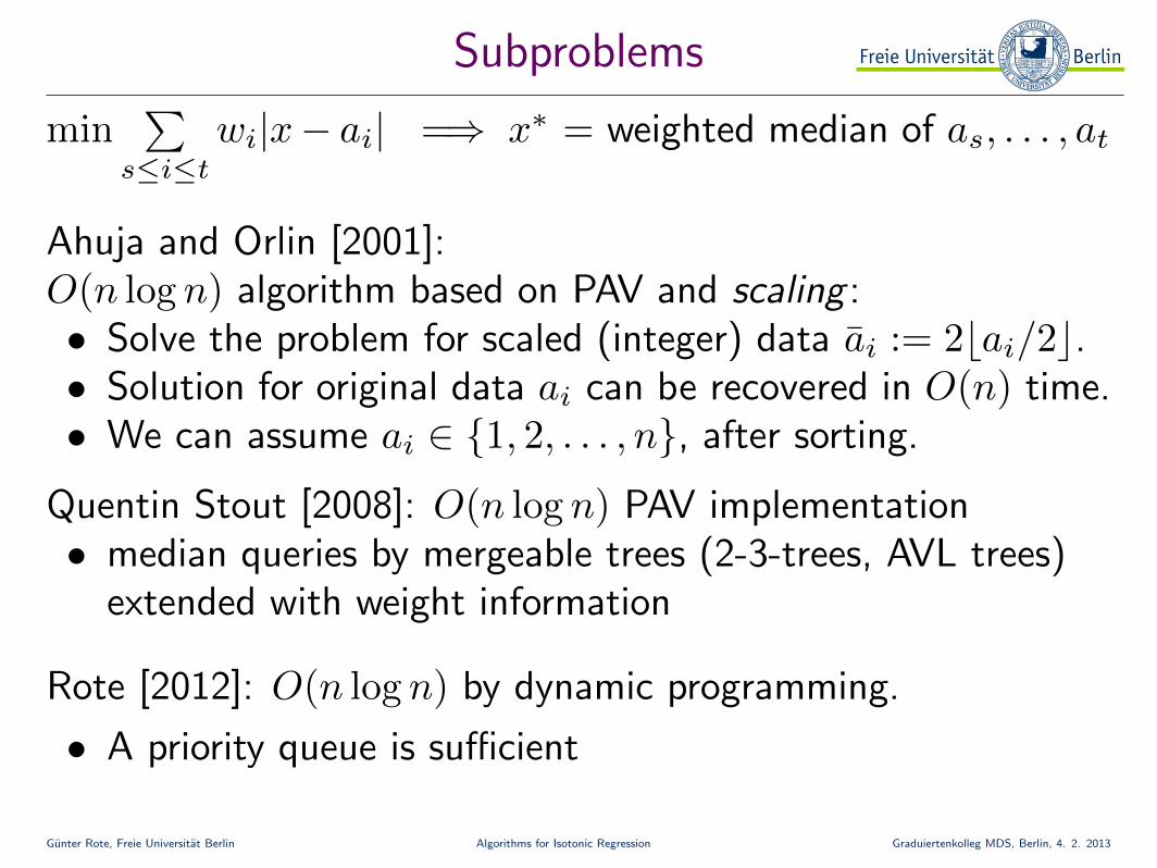
s≤i≤twi|x− ai| =⇒ x∗ = weighted median of as, . . . , at
Ahuja and Orlin [2001]:O(n log n) algorithm based on PAV and scaling :• Solve the problem for scaled (integer) data ai := 2bai/2c.• Solution for original data ai can be recovered in O(n) time.• We can assume ai ∈ {1, 2, . . . , n}, after sorting.
Quentin Stout [2008]: O(n log n) PAV implementation• median queries by mergeable trees (2-3-trees, AVL trees)
extended with weight information
Rote [2012]: O(n log n) by dynamic programming.
• A priority queue is sufficient
Gunter Rote, Freie Universitat Berlin Algorithms for Isotonic Regression Graduiertenkolleg MDS, Berlin, 4. 2. 2013
Dynamic programming
Rekursion:
fk(z) := min{ fk−1(x) : x ≤ z }+ wk · |z − ak|
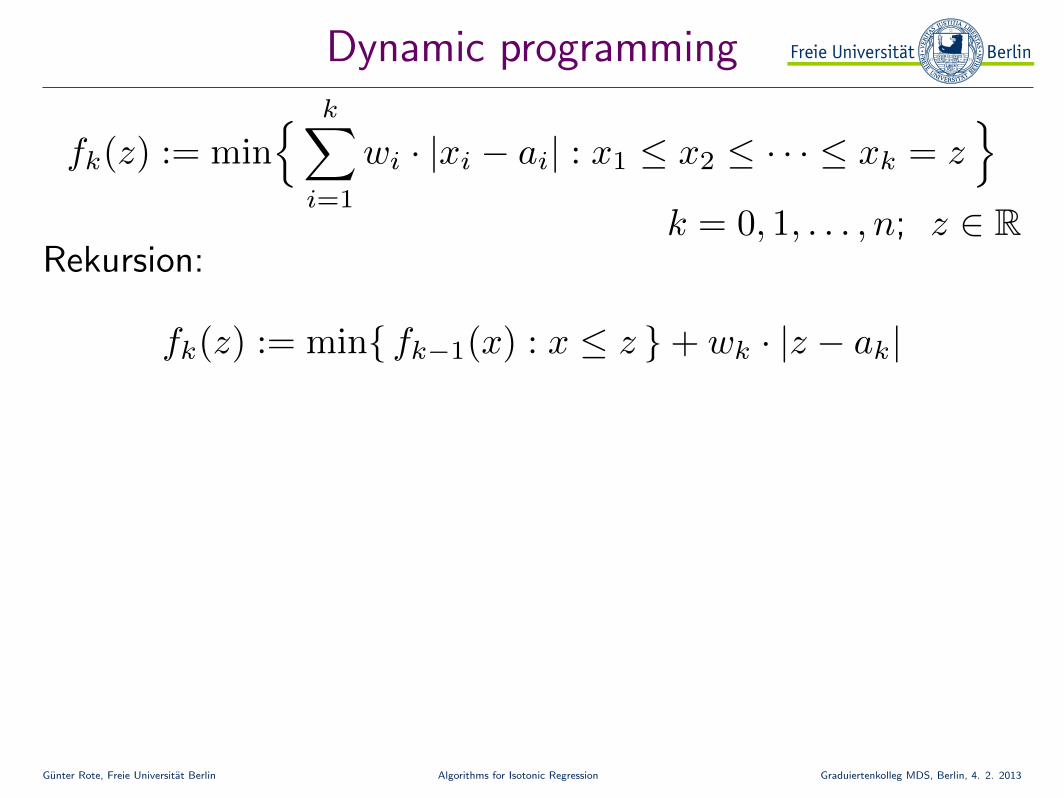
fk(z) := min{ k∑
i=1
wi · |xi − ai| : x1 ≤ x2 ≤ · · · ≤ xk = z}
k = 0, 1, . . . , n; z ∈ R
Gunter Rote, Freie Universitat Berlin Algorithms for Isotonic Regression Graduiertenkolleg MDS, Berlin, 4. 2. 2013
Dynamic programming
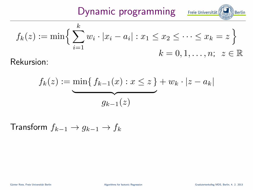
Rekursion:
fk(z) := min{ fk−1(x) : x ≤ z }+ wk · |z − ak|
fk(z) := min{ k∑
i=1
wi · |xi − ai| : x1 ≤ x2 ≤ · · · ≤ xk = z}
k = 0, 1, . . . , n; z ∈ R
︸ ︷︷ ︸gk−1(z)
Transform fk−1 → gk−1 → fk
Gunter Rote, Freie Universitat Berlin Algorithms for Isotonic Regression Graduiertenkolleg MDS, Berlin, 4. 2. 2013
Recursion step 1
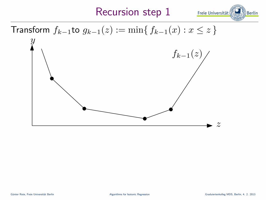
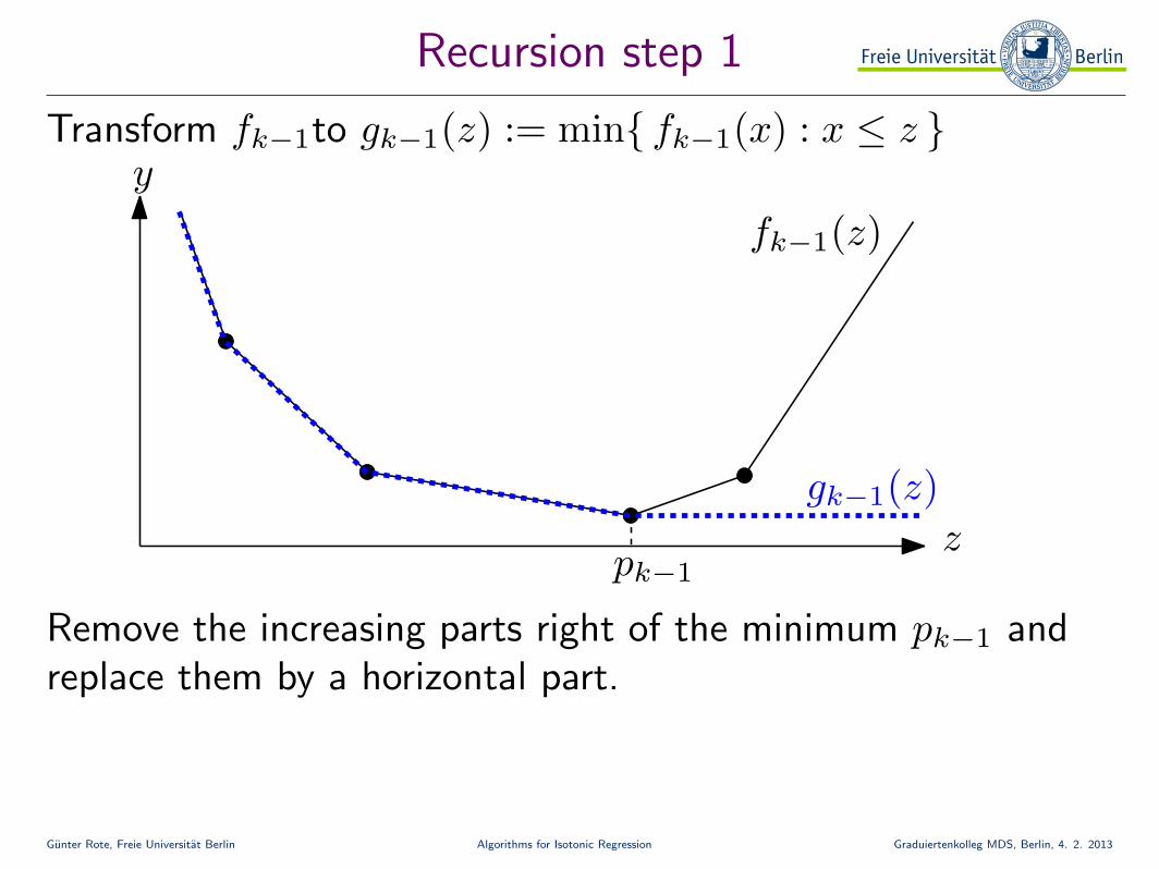
Transform fk−1to gk−1(z) := min{ fk−1(x) : x ≤ z }
fk−1(z)
z
y
Gunter Rote, Freie Universitat Berlin Algorithms for Isotonic Regression Graduiertenkolleg MDS, Berlin, 4. 2. 2013
Recursion step 1
Transform fk−1to gk−1(z) := min{ fk−1(x) : x ≤ z }
fk−1(z)
z
y
pk−1
gk−1(z)
Remove the increasing parts right of the minimum pk−1 andreplace them by a horizontal part.
Gunter Rote, Freie Universitat Berlin Algorithms for Isotonic Regression Graduiertenkolleg MDS, Berlin, 4. 2. 2013
Recursion step 2
Transform gk−1 to fk(z) = gk−1(z) + wk · |z − ak|• Add two convex piecewise-linear functions
Gunter Rote, Freie Universitat Berlin Algorithms for Isotonic Regression Graduiertenkolleg MDS, Berlin, 4. 2. 2013
Recursion step 2
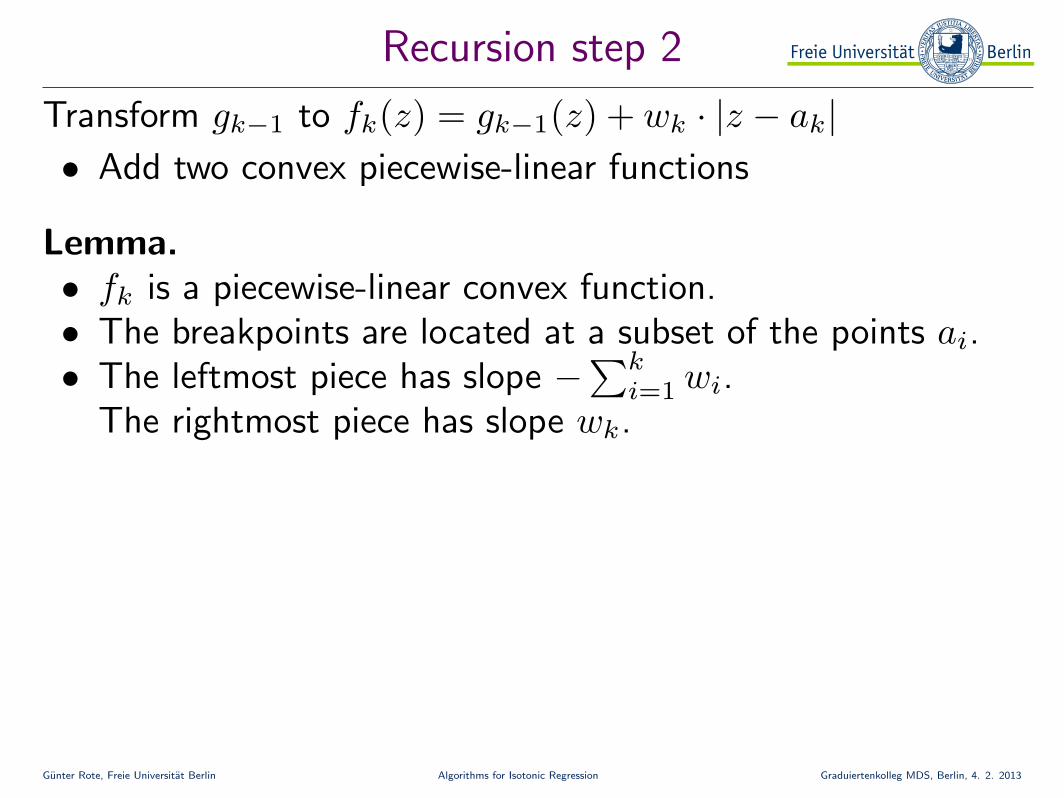
Transform gk−1 to fk(z) = gk−1(z) + wk · |z − ak|• Add two convex piecewise-linear functions
Lemma.• fk is a piecewise-linear convex function.• The breakpoints are located at a subset of the points ai.• The leftmost piece has slope −
∑ki=1 wi.
The rightmost piece has slope wk.
Gunter Rote, Freie Universitat Berlin Algorithms for Isotonic Regression Graduiertenkolleg MDS, Berlin, 4. 2. 2013
Piecewise-linear functions
x
y = s′x + t′
y = s′′x + t′′y = sx + t
x0
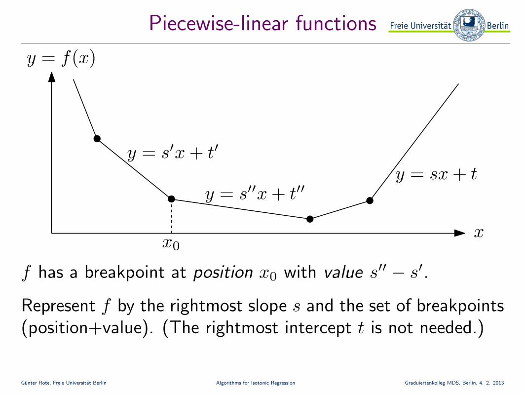
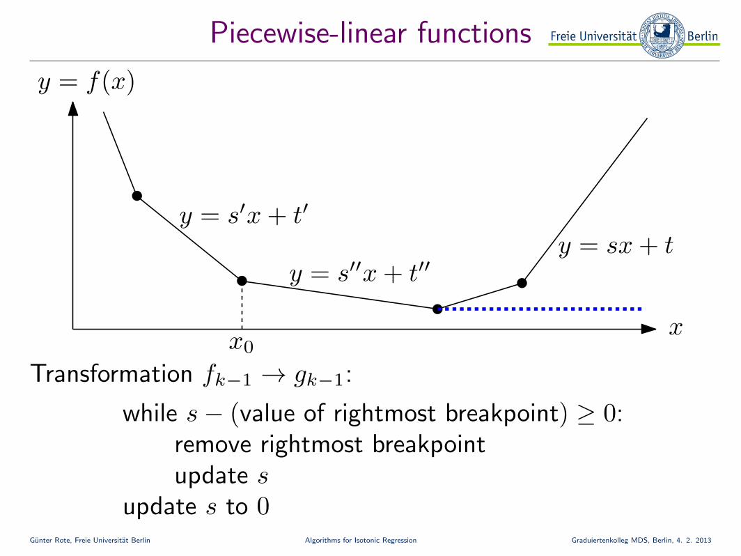
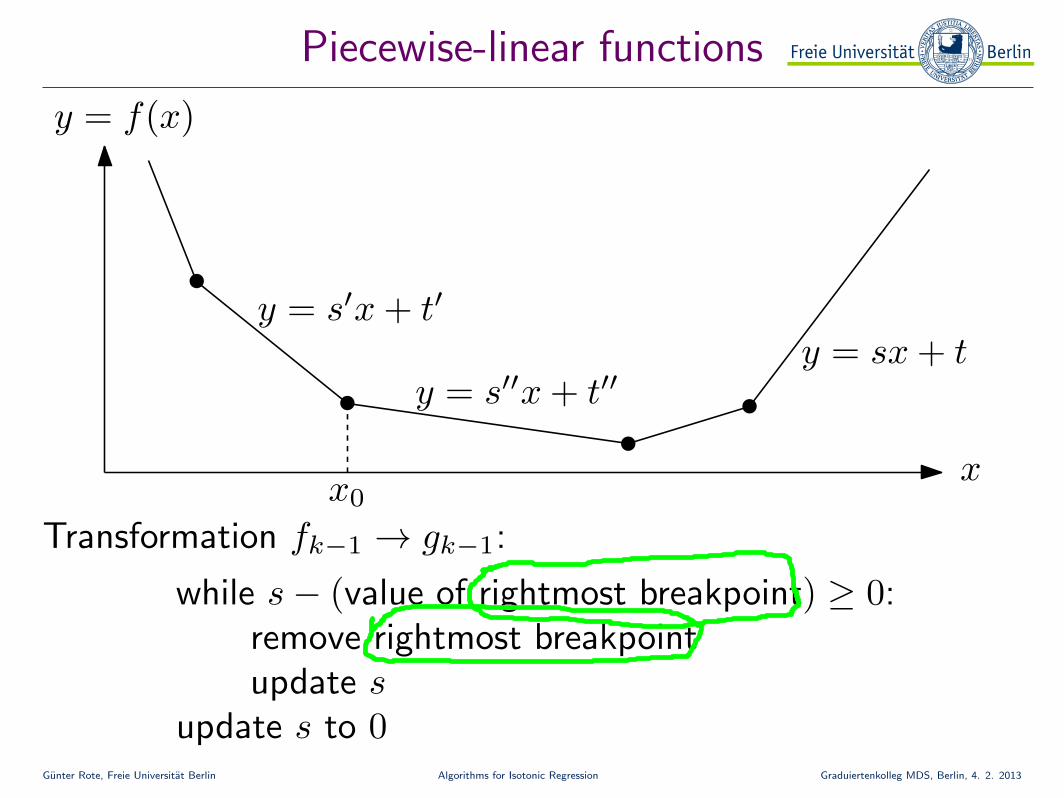
f has a breakpoint at position x0 with value s′′ − s′.
Represent f by the rightmost slope s and the set of breakpoints(position+value). (The rightmost intercept t is not needed.)
y = f(x)
Gunter Rote, Freie Universitat Berlin Algorithms for Isotonic Regression Graduiertenkolleg MDS, Berlin, 4. 2. 2013
Piecewise-linear functions
x
y = s′x + t′
y = s′′x + t′′y = sx + t
x0
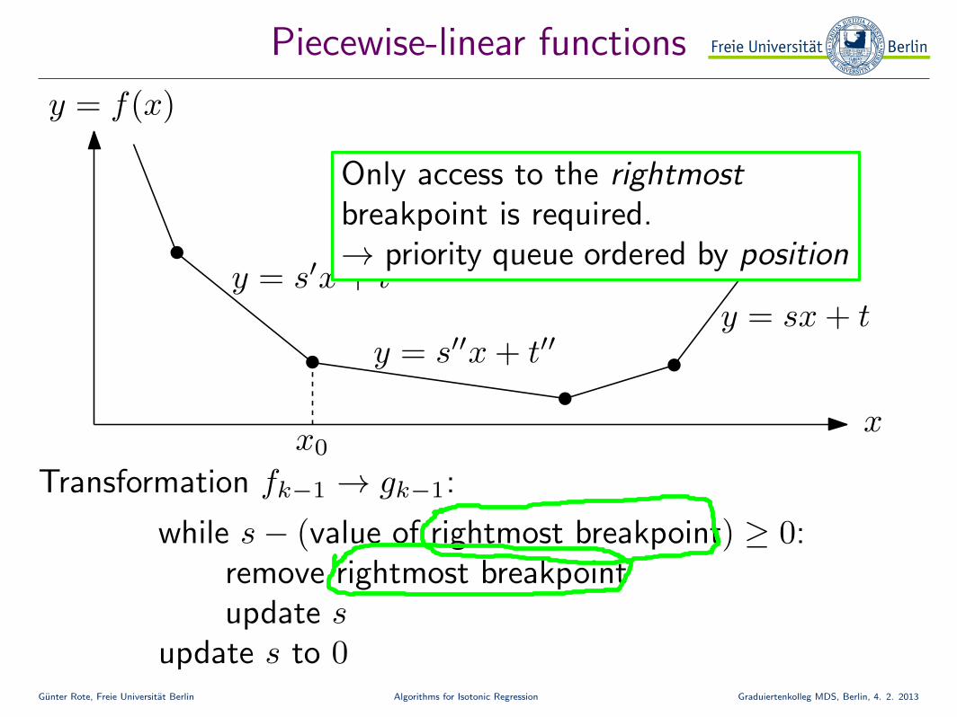
Transformation fk−1 → gk−1:
while s− (value of rightmost breakpoint) ≥ 0:remove rightmost breakpointupdate s
update s to 0
y = f(x)
Gunter Rote, Freie Universitat Berlin Algorithms for Isotonic Regression Graduiertenkolleg MDS, Berlin, 4. 2. 2013
Piecewise-linear functions
x
y = s′x + t′
y = s′′x + t′′y = sx + t
x0
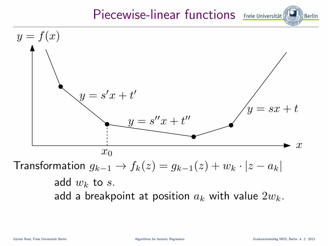
Transformation gk−1 → fk(z) = gk−1(z) + wk · |z − ak|add wk to s.add a breakpoint at position ak with value 2wk.
y = f(x)
Gunter Rote, Freie Universitat Berlin Algorithms for Isotonic Regression Graduiertenkolleg MDS, Berlin, 4. 2. 2013
Piecewise-linear functions
x
y = s′x + t′
y = s′′x + t′′y = sx + t
x0
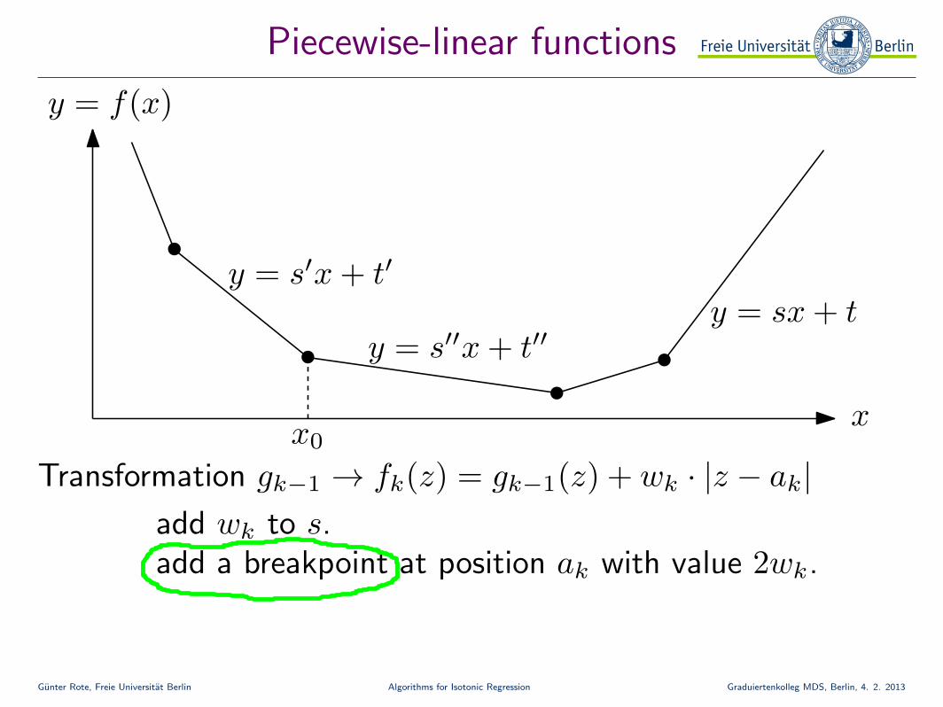
Transformation gk−1 → fk(z) = gk−1(z) + wk · |z − ak|add wk to s.add a breakpoint at position ak with value 2wk.
y = f(x)
Gunter Rote, Freie Universitat Berlin Algorithms for Isotonic Regression Graduiertenkolleg MDS, Berlin, 4. 2. 2013
Piecewise-linear functions
x
y = s′x + t′
y = s′′x + t′′y = sx + t
x0
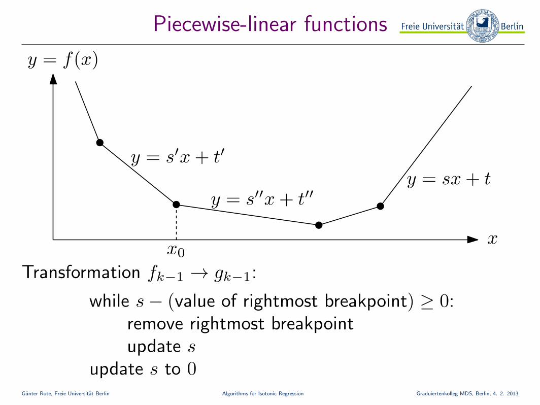
Transformation fk−1 → gk−1:
while s− (value of rightmost breakpoint) ≥ 0:remove rightmost breakpointupdate s
update s to 0
y = f(x)
Gunter Rote, Freie Universitat Berlin Algorithms for Isotonic Regression Graduiertenkolleg MDS, Berlin, 4. 2. 2013
Piecewise-linear functions
x
y = s′x + t′
y = s′′x + t′′y = sx + t
x0
Transformation fk−1 → gk−1:
while s− (value of rightmost breakpoint) ≥ 0:remove rightmost breakpointupdate s
update s to 0
y = f(x)
Only access to the rightmostbreakpoint is required.→ priority queue ordered by position
Gunter Rote, Freie Universitat Berlin Algorithms for Isotonic Regression Graduiertenkolleg MDS, Berlin, 4. 2. 2013
The algorithm
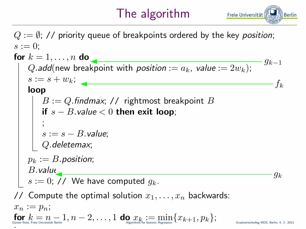
Q := ∅; // priority queue of breakpoints ordered by the key position;s := 0;for k = 1, . . . , n do // On entry, Q and s represents gk−1.
Q.add(new breakpoint with position := ak, value := 2wk);s := s + wk; // We have computed fk.while true do
B := Q.findmax; // rightmost breakpoint Bif s−B.value < 0 then exit loop;;s := s−B.value;Q.deletemax;
pk := B.position;B.value := B.value− s;s := 0; // We have computed gk.
// Compute the optimal solution x1, . . . , xn backwards:xn := pn;for k = n− 1, n− 2, . . . , 1 do xk := min{xk+1, pk};;
gk
fk
gk−1
loop
Gunter Rote, Freie Universitat Berlin Algorithms for Isotonic Regression Graduiertenkolleg MDS, Berlin, 4. 2. 2013
General objective functions
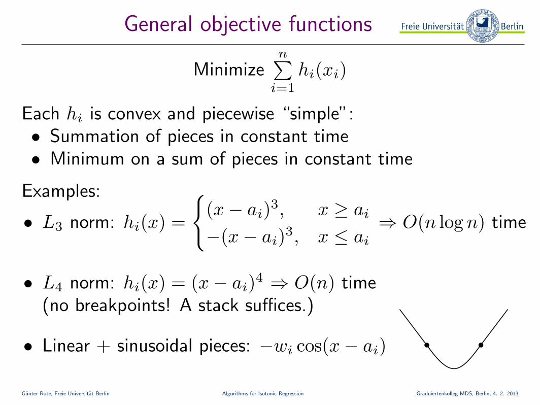
Minimizen∑
i=1
hi(xi)
Each hi is convex and piecewise “simple”:• Summation of pieces in constant time• Minimum on a sum of pieces in constant time
• L3 norm: hi(x) =
{(x− ai)
3, x ≥ ai
−(x− ai)3, x ≤ ai
⇒ O(n log n) time
Examples:
• L4 norm: hi(x) = (x− ai)4 ⇒ O(n) time
(no breakpoints! A stack suffices.)
• Linear + sinusoidal pieces: −wi cos(x− ai)
Gunter Rote, Freie Universitat Berlin Algorithms for Isotonic Regression Graduiertenkolleg MDS, Berlin, 4. 2. 2013
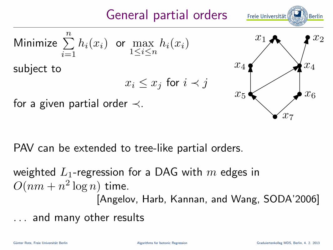
General partial orders
subject toxi ≤ xj for i ≺ j
for a given partial order ≺.
Minimizen∑
i=1
hi(xi) or max1≤i≤n
hi(xi)x1
x6
x7
x5
x4
x2
x4
PAV can be extended to tree-like partial orders.
weighted L1-regression for a DAG with m edges inO(nm + n2 log n) time.
[Angelov, Harb, Kannan, and Wang, SODA’2006]
. . . and many other results
Gunter Rote, Freie Universitat Berlin Algorithms for Isotonic Regression Graduiertenkolleg MDS, Berlin, 4. 2. 2013
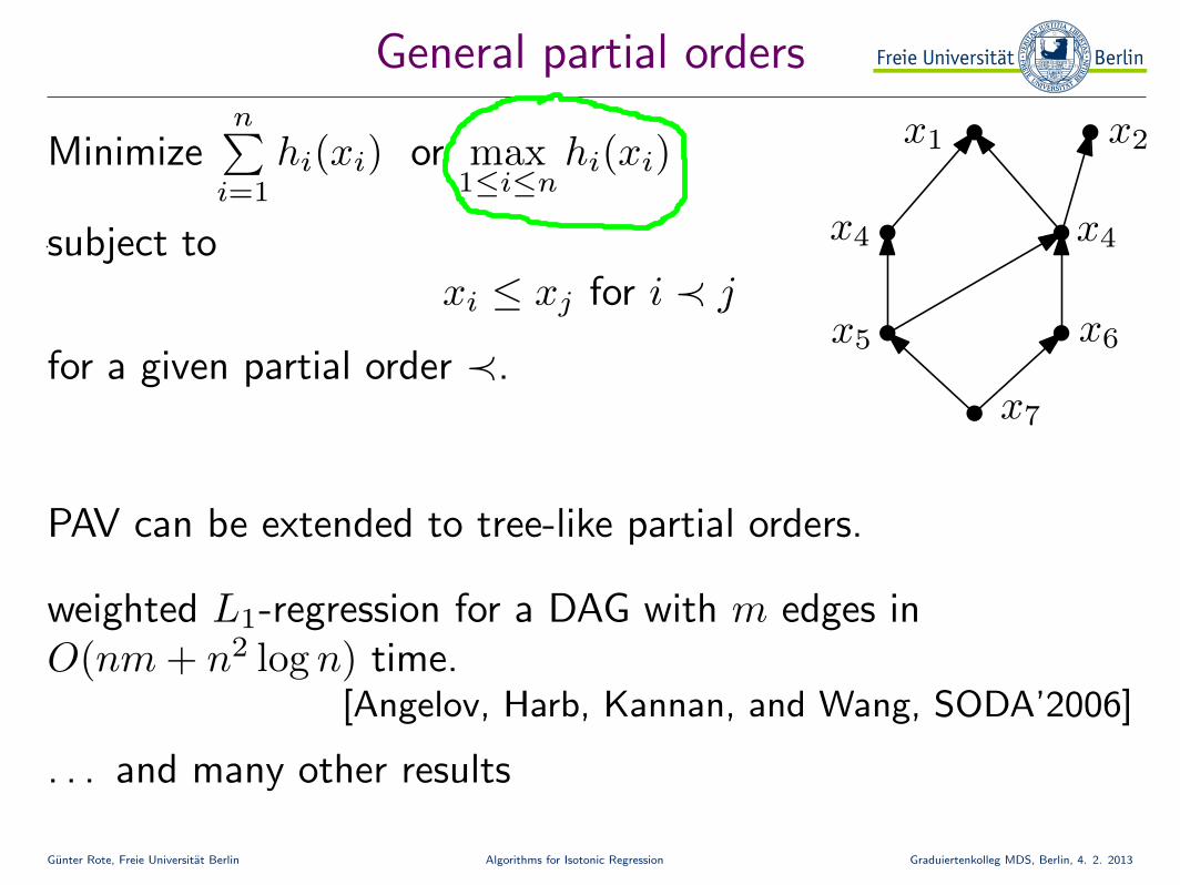
General partial orders
subject toxi ≤ xj for i ≺ j
for a given partial order ≺.
Minimizen∑
i=1
hi(xi) or max1≤i≤n
hi(xi)x1
x6
x7
x5
x4
x2
x4
PAV can be extended to tree-like partial orders.
weighted L1-regression for a DAG with m edges inO(nm + n2 log n) time.
[Angelov, Harb, Kannan, and Wang, SODA’2006]
. . . and many other results
Gunter Rote, Freie Universitat Berlin Algorithms for Isotonic Regression Graduiertenkolleg MDS, Berlin, 4. 2. 2013
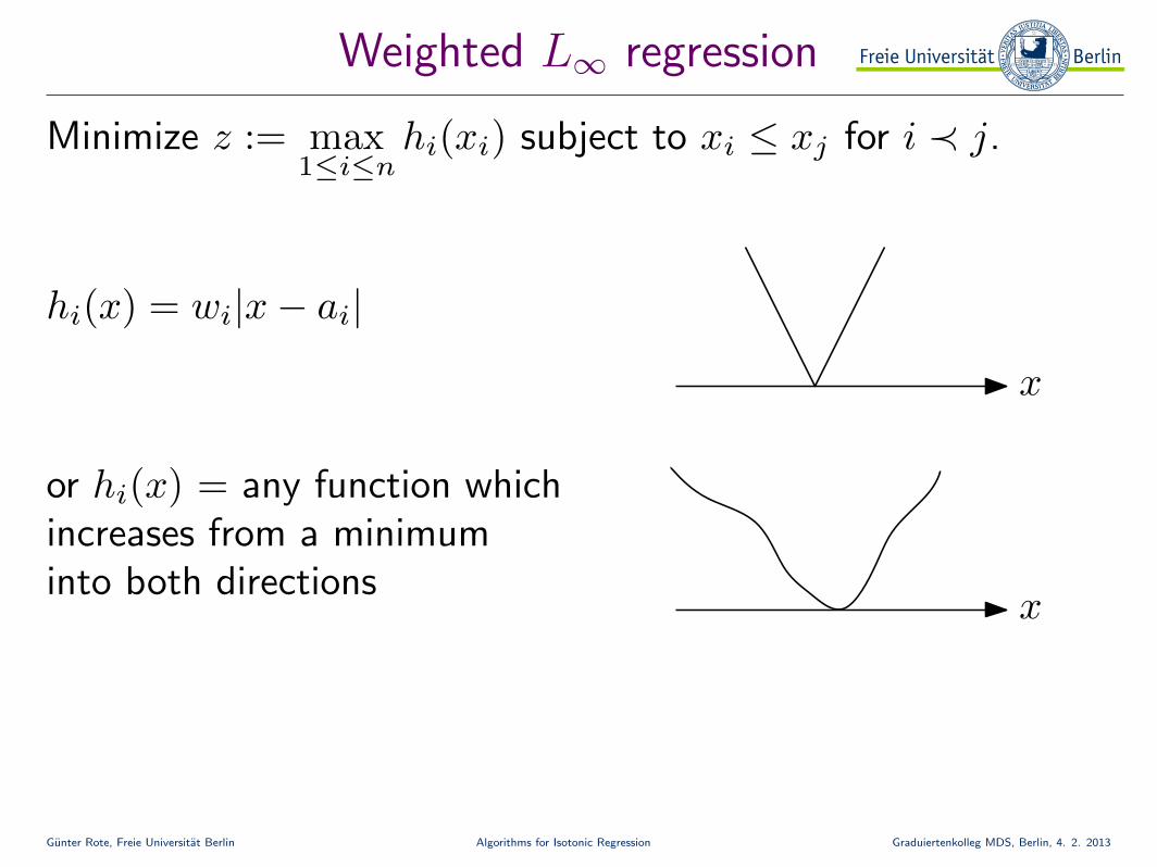
Weighted L∞ regression
x
Minimize z := max1≤i≤n
hi(xi) subject to xi ≤ xj for i ≺ j.
hi(x) = wi|x− ai|
or hi(x) = any function whichincreases from a minimuminto both directions
x
Gunter Rote, Freie Universitat Berlin Algorithms for Isotonic Regression Graduiertenkolleg MDS, Berlin, 4. 2. 2013
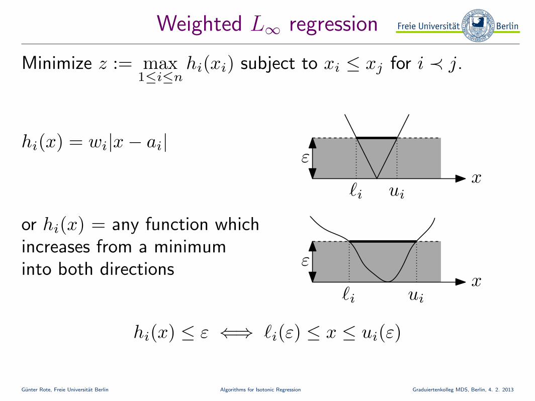
Weighted L∞ regression
xε
Minimize z := max1≤i≤n
hi(xi) subject to xi ≤ xj for i ≺ j.
hi(x) = wi|x− ai|
or hi(x) = any function whichincreases from a minimuminto both directions
x
hi(x) ≤ ε ⇐⇒ `i(ε) ≤ x ≤ ui(ε)
ε
`i ui
ui`i
Gunter Rote, Freie Universitat Berlin Algorithms for Isotonic Regression Graduiertenkolleg MDS, Berlin, 4. 2. 2013
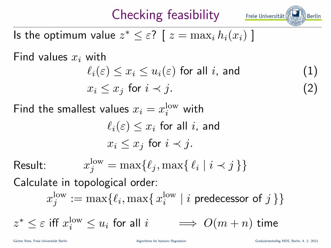
Checking feasibility
`i(ε) ≤ xi ≤ ui(ε) for all i, and (1)
xi ≤ xj for i ≺ j. (2)
Is the optimum value z∗ ≤ ε? [ z = maxi hi(xi) ]
`i(ε) ≤ xi for all i, and
xi ≤ xj for i ≺ j.
Find values xi with
Find the smallest values xi = xlowi with
xlowj := max{`i,max{xlow
i | i predecessor of j }}
z∗ ≤ ε iff xlowi ≤ ui for all i =⇒ O(m + n) time
xlowj = max{`j ,max{ `i | i ≺ j }}
Calculate in topological order:
Result:
Gunter Rote, Freie Universitat Berlin Algorithms for Isotonic Regression Graduiertenkolleg MDS, Berlin, 4. 2. 2013
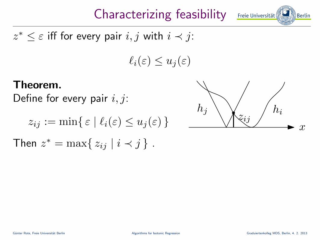
Characterizing feasibility
z∗ ≤ ε iff for every pair i, j with i ≺ j:
`i(ε) ≤ uj(ε)
zij := min{ ε | `i(ε) ≤ uj(ε) } x
hihj
Theorem.Define for every pair i, j:
zij
Then z∗ = max{ zij | i ≺ j } .
Gunter Rote, Freie Universitat Berlin Algorithms for Isotonic Regression Graduiertenkolleg MDS, Berlin, 4. 2. 2013
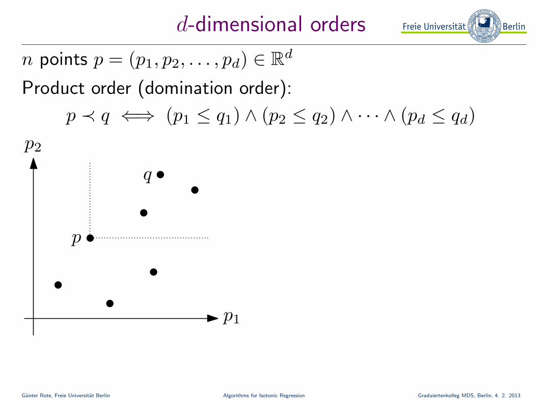
d-dimensional orders
n points p = (p1, p2, . . . , pd) ∈ Rd
p ≺ q ⇐⇒ (p1 ≤ q1) ∧ (p2 ≤ q2) ∧ · · · ∧ (pd ≤ qd)
Product order (domination order):
p2
p1
p
q
Gunter Rote, Freie Universitat Berlin Algorithms for Isotonic Regression Graduiertenkolleg MDS, Berlin, 4. 2. 2013
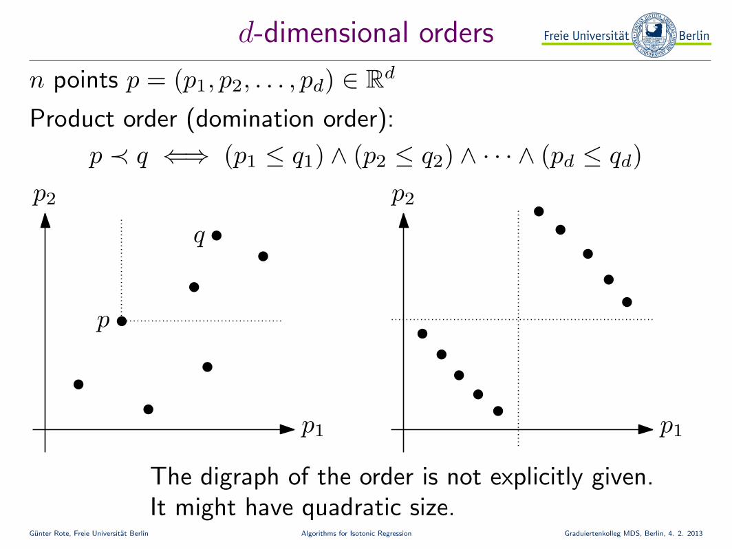
d-dimensional orders
n points p = (p1, p2, . . . , pd) ∈ Rd
p ≺ q ⇐⇒ (p1 ≤ q1) ∧ (p2 ≤ q2) ∧ · · · ∧ (pd ≤ qd)
Product order (domination order):
p2
p1
p
q
p2
p1
The digraph of the order is not explicitly given.It might have quadratic size.
Gunter Rote, Freie Universitat Berlin Algorithms for Isotonic Regression Graduiertenkolleg MDS, Berlin, 4. 2. 2013
L∞ regression for d-dimensional orders
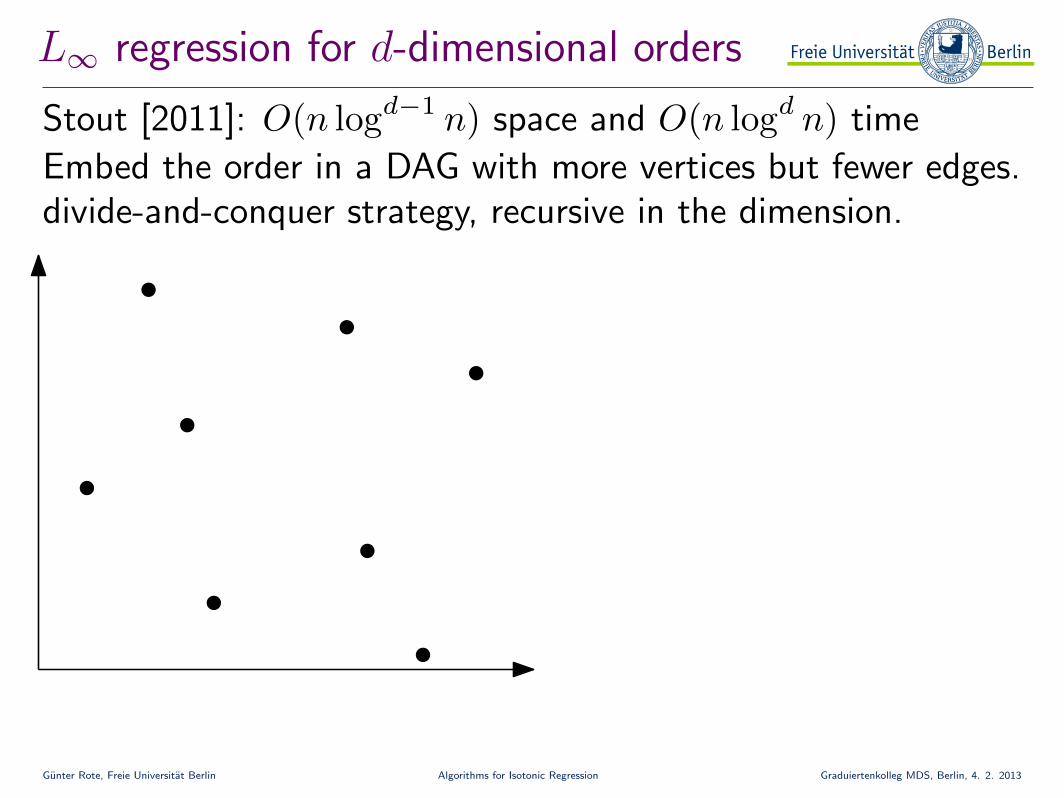
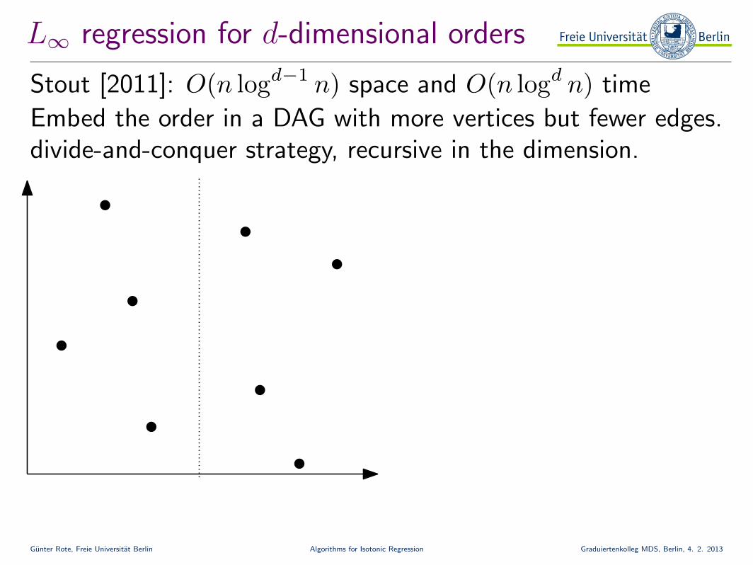
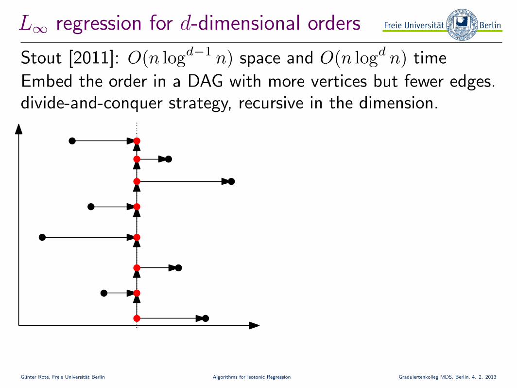
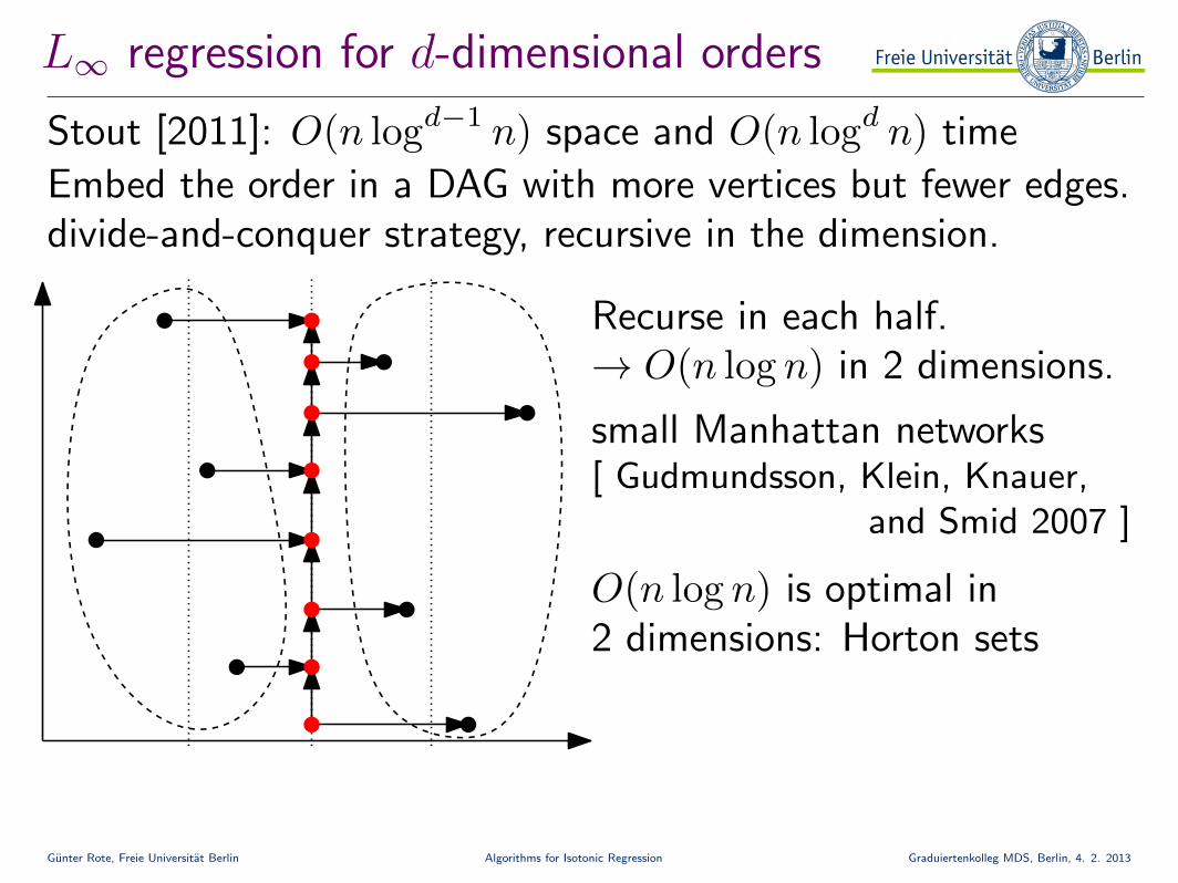
Stout [2011]: O(n logd−1 n) space and O(n logd n) time
Embed the order in a DAG with more vertices but fewer edges.divide-and-conquer strategy, recursive in the dimension.
Gunter Rote, Freie Universitat Berlin Algorithms for Isotonic Regression Graduiertenkolleg MDS, Berlin, 4. 2. 2013
L∞ regression for d-dimensional orders
Stout [2011]: O(n logd−1 n) space and O(n logd n) time
Embed the order in a DAG with more vertices but fewer edges.divide-and-conquer strategy, recursive in the dimension.
Recurse in each half.→ O(n log n) in 2 dimensions.
O(n log n) is optimal in2 dimensions: Horton sets
small Manhattan networks[ Gudmundsson, Klein, Knauer,
and Smid 2007 ]
Gunter Rote, Freie Universitat Berlin Algorithms for Isotonic Regression Graduiertenkolleg MDS, Berlin, 4. 2. 2013
L∞ regression for d-dimensional orders
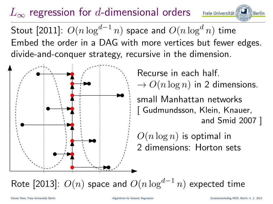
Stout [2011]: O(n logd−1 n) space and O(n logd n) time
Rote [2013]: O(n) space and O(n logd−1 n) expected time
Embed the order in a DAG with more vertices but fewer edges.divide-and-conquer strategy, recursive in the dimension.
Recurse in each half.→ O(n log n) in 2 dimensions.
O(n log n) is optimal in2 dimensions: Horton sets
small Manhattan networks[ Gudmundsson, Klein, Knauer,
and Smid 2007 ]
Gunter Rote, Freie Universitat Berlin Algorithms for Isotonic Regression Graduiertenkolleg MDS, Berlin, 4. 2. 2013
L∞ regression for d-dimensional orders
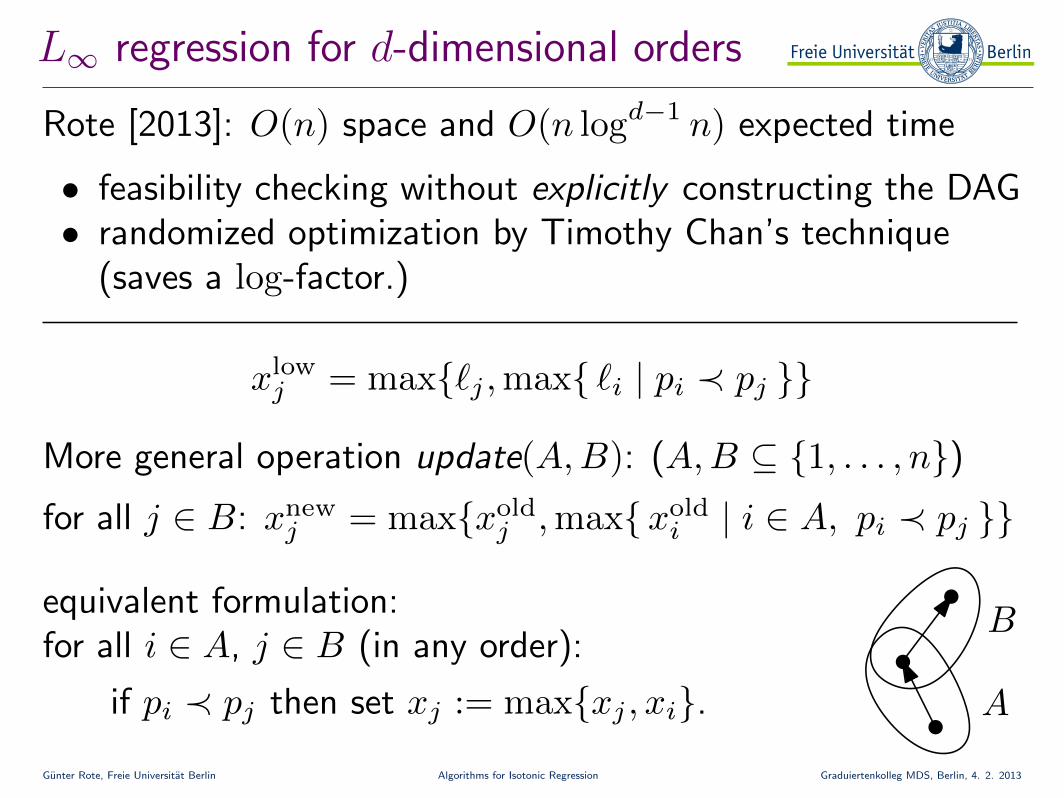
Rote [2013]: O(n) space and O(n logd−1 n) expected time
• feasibility checking without explicitly constructing the DAG• randomized optimization by Timothy Chan’s technique
(saves a log-factor.)
xlowj = max{`j ,max{ `i | pi ≺ pj }}
More general operation update(A,B): (A,B ⊆ {1, . . . , n})for all j ∈ B: xnew
j = max{xoldj ,max{xold
i | i ∈ A, pi ≺ pj }}
equivalent formulation:for all i ∈ A, j ∈ B (in any order):
if pi ≺ pj then set xj := max{xj , xi}. A
B

Gunter Rote, Freie Universitat Berlin Algorithms for Isotonic Regression Graduiertenkolleg MDS, Berlin, 4. 2. 2013
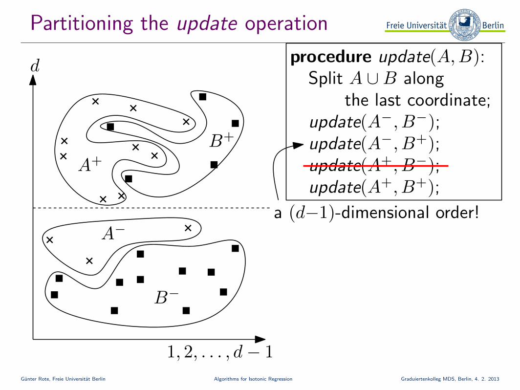
Partitioning the update operation
A−
A+
B+
B−
1, 2, . . . , d− 1
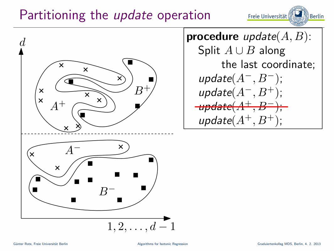
dprocedure update(A,B):
Split A ∪B alongthe last coordinate;
update(A−, B−);update(A−, B+);update(A+, B−);update(A+, B+);
Gunter Rote, Freie Universitat Berlin Algorithms for Isotonic Regression Graduiertenkolleg MDS, Berlin, 4. 2. 2013
Partitioning the update operation
A−
A+
B+
B−
1, 2, . . . , d− 1
dprocedure update(A,B):
Split A ∪B alongthe last coordinate;
update(A−, B−);update(A−, B+);update(A+, B−);update(A+, B+);
a (d−1)-dimensional order!
Gunter Rote, Freie Universitat Berlin Algorithms for Isotonic Regression Graduiertenkolleg MDS, Berlin, 4. 2. 2013
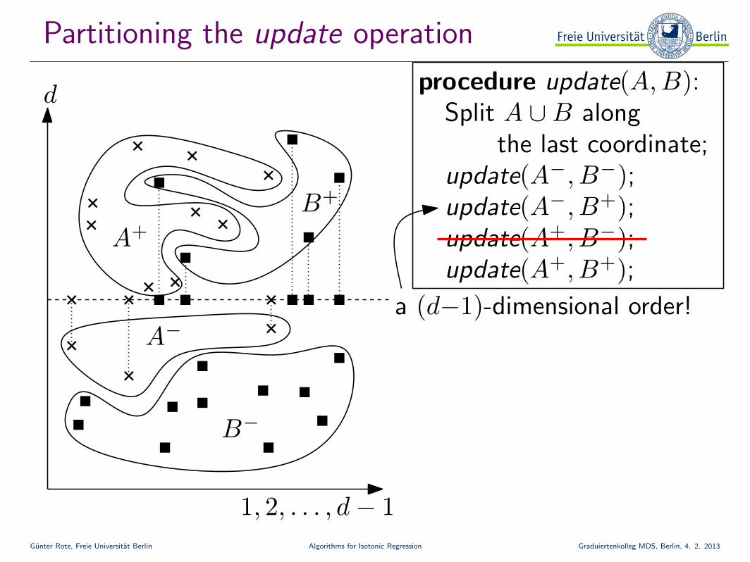
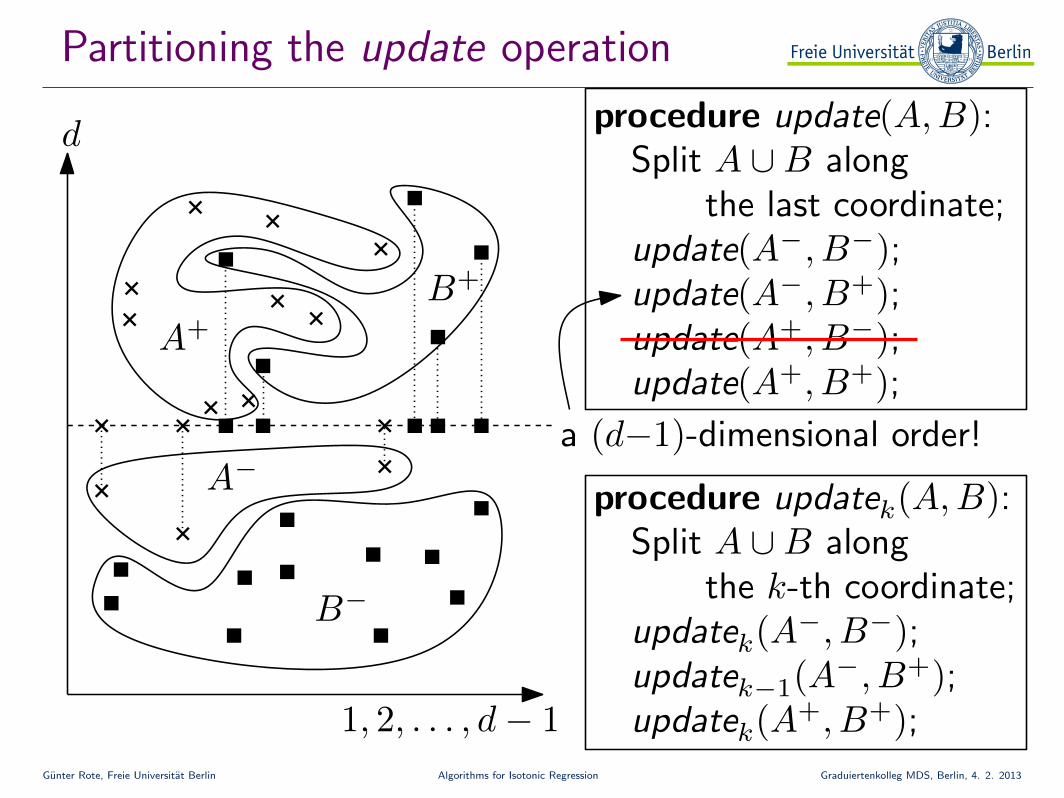
Partitioning the update operation
A−
A+
B+
B−
1, 2, . . . , d− 1
dprocedure update(A,B):
Split A ∪B alongthe last coordinate;
update(A−, B−);update(A−, B+);update(A+, B−);update(A+, B+);
a (d−1)-dimensional order!
procedure updatek(A,B):Split A ∪B along
the k-th coordinate;updatek(A−, B−);updatek−1(A−, B+);updatek(A+, B+);
Gunter Rote, Freie Universitat Berlin Algorithms for Isotonic Regression Graduiertenkolleg MDS, Berlin, 4. 2. 2013
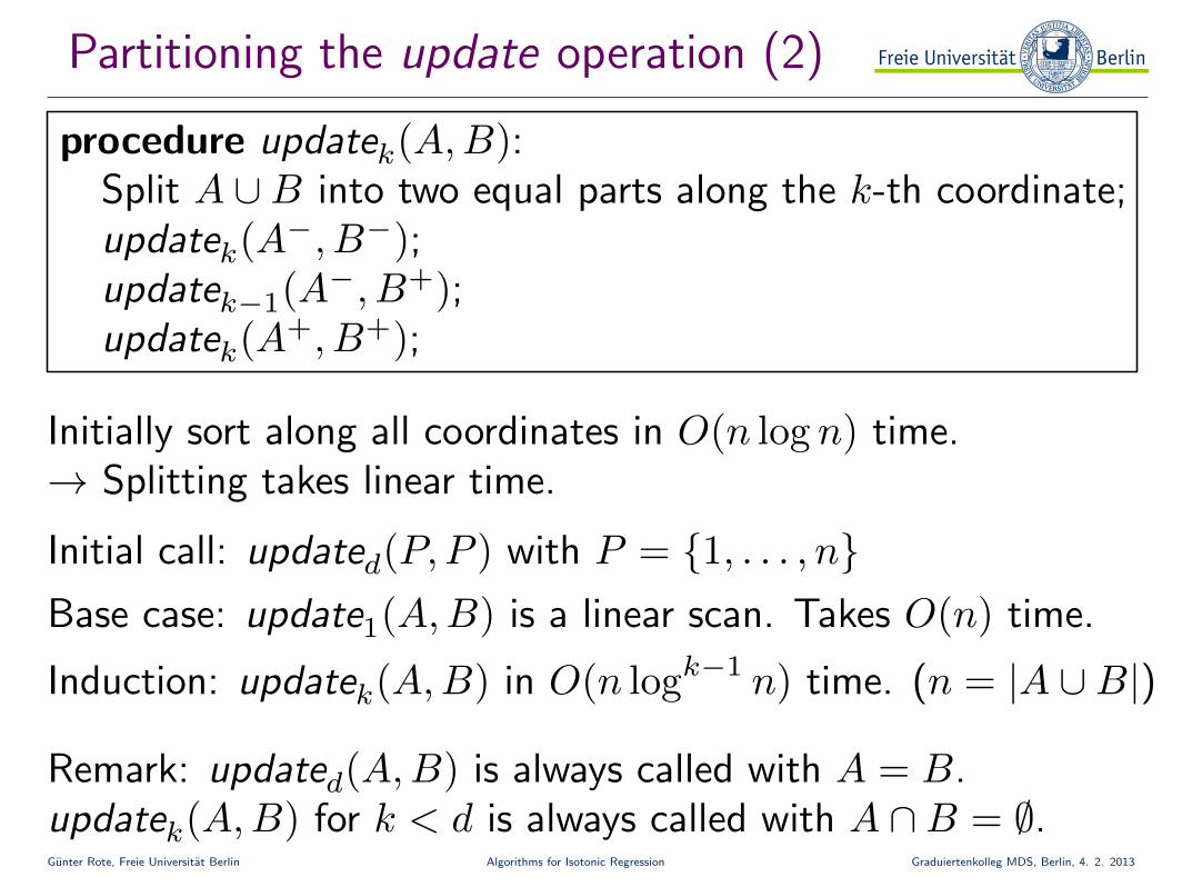
Partitioning the update operation (2)
procedure updatek(A,B):Split A ∪B into two equal parts along the k-th coordinate;updatek(A−, B−);updatek−1(A−, B+);updatek(A+, B+);
Base case: update1(A,B) is a linear scan. Takes O(n) time.
Initially sort along all coordinates in O(n log n) time.→ Splitting takes linear time.
Initial call: updated(P, P ) with P = {1, . . . , n}
Induction: updatek(A,B) in O(n logk−1 n) time. (n = |A ∪B|)
Remark: updated(A,B) is always called with A = B.updatek(A,B) for k < d is always called with A ∩B = ∅.
Gunter Rote, Freie Universitat Berlin Algorithms for Isotonic Regression Graduiertenkolleg MDS, Berlin, 4. 2. 2013
Randomized optimization technique
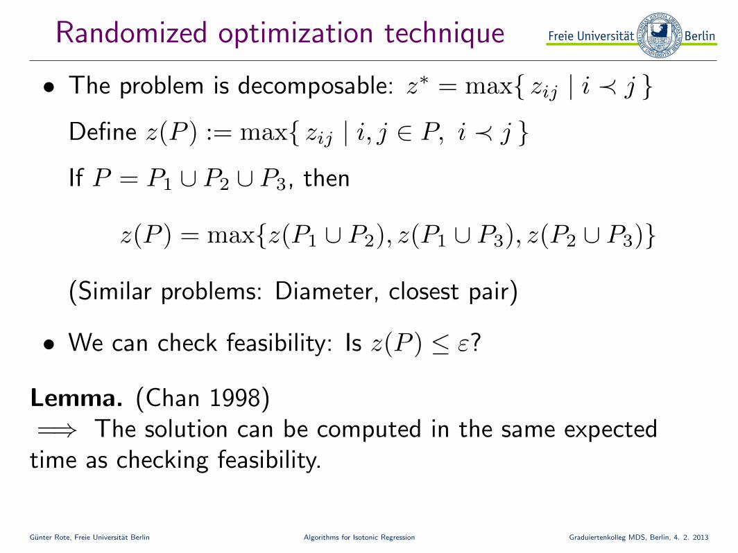
• The problem is decomposable: z∗ = max{ zij | i ≺ j }
Define z(P ) := max{ zij | i, j ∈ P, i ≺ j }
If P = P1 ∪ P2 ∪ P3, then
z(P ) = max{z(P1 ∪ P2), z(P1 ∪ P3), z(P2 ∪ P3)}
(Similar problems: Diameter, closest pair)
• We can check feasibility: Is z(P ) ≤ ε?
Lemma. (Chan 1998)=⇒ The solution can be computed in the same expected
time as checking feasibility.
Gunter Rote, Freie Universitat Berlin Algorithms for Isotonic Regression Graduiertenkolleg MDS, Berlin, 4. 2. 2013
Randomized maximization
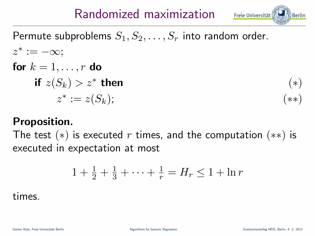
Permute subproblems S1, S2, . . . , Sr into random order.
z∗ := −∞;
for k = 1, . . . , r do
if z(Sk) > z∗ then (∗)z∗ := z(Sk); (∗∗)
Proposition.The test (∗) is executed r times, and the computation (∗∗) isexecuted in expectation at most
1 + 12 + 1
3 + · · ·+ 1r = Hr ≤ 1 + ln r
times.
Gunter Rote, Freie Universitat Berlin Algorithms for Isotonic Regression Graduiertenkolleg MDS, Berlin, 4. 2. 2013
L∞ regression in d dimensions
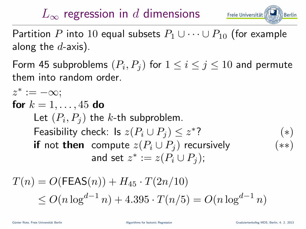
Partition P into 10 equal subsets P1 ∪ · · · ∪ P10 (for examplealong the d-axis).
Form 45 subproblems (Pi, Pj) for 1 ≤ i ≤ j ≤ 10 and permutethem into random order.
z∗ := −∞;for k = 1, . . . , 45 do
Let (Pi, Pj) the k-th subproblem.
if not then compute z(Pi ∪ Pj) recursivelyand set z∗ := z(Pi ∪ Pj);
(∗∗)Feasibility check: Is z(Pi ∪ Pj) ≤ z∗? (∗)
T (n) = O(FEAS(n)) + H45 · T (2n/10)
≤ O(n logd−1 n) + 4.395 · T (n/5) = O(n logd−1 n)