Isotonic Regression in General Dimensions

Sabyasachi ChatterjeeDepartment of Statistics

University of Illinois at Urbana-Champaign

29 January 2018

1 / 30

References

1. S.Chatterjee, A. Guntuboyina and B. Sen (2015) On RiskBounds in Isotonic and Other Shape ConstrainedRegression Problems

2. S.Chatterjee, A. Guntuboyina and B. Sen (2016) On MatrixEstimation under Monotonicity Constraints

3. S.Chatterjee, Roy Han, Tengyao Wang and Richard Samworth(2017) Isotonic Regression in General Dimensions

2 / 30

Outline

1. Isotonic Regression– Definition

2. Minimax Rate Optimality of the LSE

3. Statistical Dimension of the Monotone Cone

4. Adaptivity of the LSE

3 / 30

Setting (Monotone Function Estimation)

We are given data

Yi = f ∗(xi ) + εi for i = 1, . . . , n

where εi ’s are i.i.d N(0, σ2) with σ2 unknown.

f ∗ : [0, 1]d → R is an unknown function which is coordinate wisemonotone non decreasing. The problem is to recover f ∗.

x1, . . . , xn ∈ [0, 1]d are design points which could be assumed to befixed or chosen i.i.d at random. In this talk, we consider the fixedlattice design case.

4 / 30

Setting (Sequence Estimation)

Let Ld ,n be the d dimensional lattice [1, . . . , k]d where k = n1/d .

Natural partial ordering on Ld ,n. We have u ≤ v iff uj ≤ vj for all1 ≤ j ≤ d .

θ∗ is monotone with respect to the natural partial order.

We are given data Y ∼ N(θ∗, σ2In×n) with σ2 unknown.

We measure the performance of an estimator θ in terms of themean squared error:

R(θ, θ∗) =1

nEθ∗‖θ − θ∗‖2

where ‖ · ‖ is Euclidean norm.

5 / 30

Least Squares Estimator

The space of monotone functions on the lattice Ld ,n is a closedconvex cone.

Md ,n = {θ ∈ Rn : θu ≤ θv for all u ≤ v ∈ Ld ,n}.

LSE is simply the Euclidean projection of Y onto the set Md ,n.

θ = ΠMd,n(Y ) = argmin

v∈Md,n

‖Y − v‖2.

How good is the LSE as an estimator of θ∗?

6 / 30

Some History

The d = 1 case is a canonical problem in Shape ConstrainedRegression and has been studied by many authors. See Brunk(1955); van Eeden (1958); van de Geer (1990); Donoho (1991);Birge and Massart (1993); Zhang (2002); Chatterjee, Guntuboyinaand Sen (2015); Bellec(2016).

The d > 1 case is much less studied. The only work we are awareof is Chatterjee, Guntuboyina and Sen (2016) who studied thed = 2 case.

The cases d > 2 have not been studied at all in the literature.

7 / 30

MINIMAX RATE OPTIMALITY OF THE LSE

8 / 30

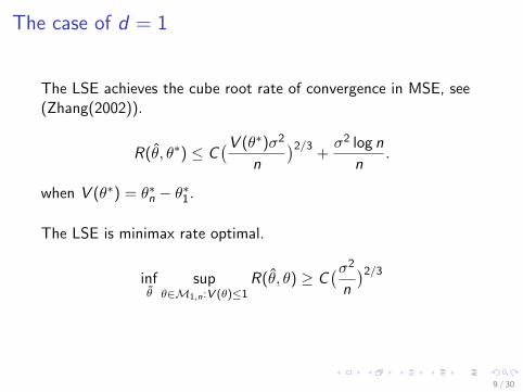
The case of d = 1

The LSE achieves the cube root rate of convergence in MSE, see(Zhang(2002)).

R(θ, θ∗) ≤ C(V (θ∗)σ2

n

)2/3+σ2 log n

n.

when V (θ∗) = θ∗n − θ∗1.

The LSE is minimax rate optimal.

infθ

supθ∈M1,n:V (θ)≤1

R(θ, θ) ≥ C(σ2n

)2/3

9 / 30

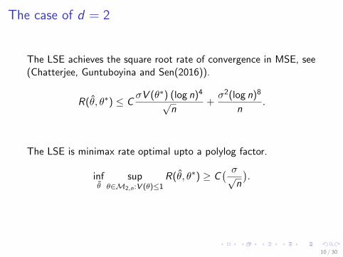
The case of d = 2

The LSE achieves the square root rate of convergence in MSE, see(Chatterjee, Guntuboyina and Sen(2016)).

R(θ, θ∗) ≤ CσV (θ∗) (log n)4√

n+σ2(log n)8

n.

The LSE is minimax rate optimal upto a polylog factor.

infθ

supθ∈M2,n:V (θ)≤1

R(θ, θ∗) ≥ C( σ√

n

).

10 / 30

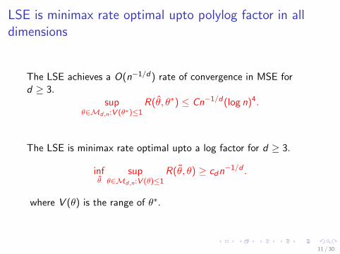
LSE is minimax rate optimal upto polylog factor in alldimensions

The LSE achieves a O(n−1/d) rate of convergence in MSE ford ≥ 3.

supθ∈Md,n:V (θ∗)≤1

R(θ, θ∗) ≤ Cn−1/d(log n)4.

The LSE is minimax rate optimal upto a log factor for d ≥ 3.

infθ

supθ∈Md,n:V (θ)≤1

R(θ, θ) ≥ cdn−1/d .

where V (θ) is the range of θ∗.

11 / 30

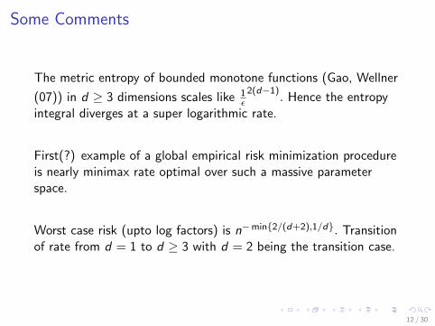
Some Comments

The metric entropy of bounded monotone functions (Gao, Wellner

(07)) in d ≥ 3 dimensions scales like 1ε

2(d−1). Hence the entropy

integral diverges at a super logarithmic rate.

First(?) example of a global empirical risk minimization procedureis nearly minimax rate optimal over such a massive parameterspace.

Worst case risk (upto log factors) is n−min{2/(d+2),1/d}. Transitionof rate from d = 1 to d ≥ 3 with d = 2 being the transition case.

12 / 30

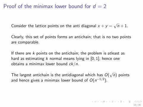
Proof of the minimax lower bound for d = 2

Consider the lattice points on the anti diagonal x + y =√n + 1.

Clearly, this set of points forms an antichain; that is no two pointsare comparable.

If there are k points on the antichain; the problem is atleast ashard as estimating k normal means lying in [0, 1]; hence oneobtains a minimax lower bound ck/n.

The largest antichain is the antidiagonal which has O(√n) points

and hence gives a minimax lower bound of O(n−1/2).

13 / 30

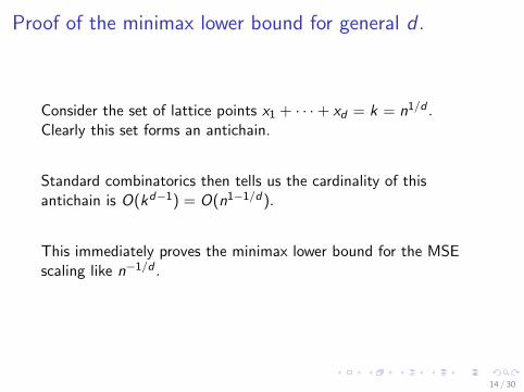
Proof of the minimax lower bound for general d .

Consider the set of lattice points x1 + · · ·+ xd = k = n1/d .Clearly this set forms an antichain.

Standard combinatorics then tells us the cardinality of thisantichain is O(kd−1) = O(n1−1/d).

This immediately proves the minimax lower bound for the MSEscaling like n−1/d .

14 / 30

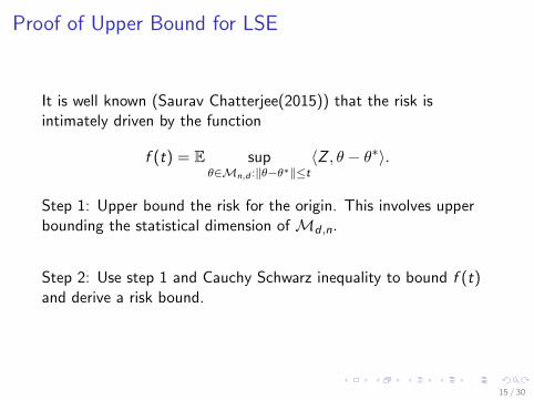
Proof of Upper Bound for LSE

It is well known (Saurav Chatterjee(2015)) that the risk isintimately driven by the function

f (t) = E supθ∈Mn,d :‖θ−θ∗‖≤t

〈Z , θ − θ∗〉.

Step 1: Upper bound the risk for the origin. This involves upperbounding the statistical dimension of Md ,n.

Step 2: Use step 1 and Cauchy Schwarz inequality to bound f (t)and derive a risk bound.

15 / 30

STATISTICAL DIMENSION

16 / 30

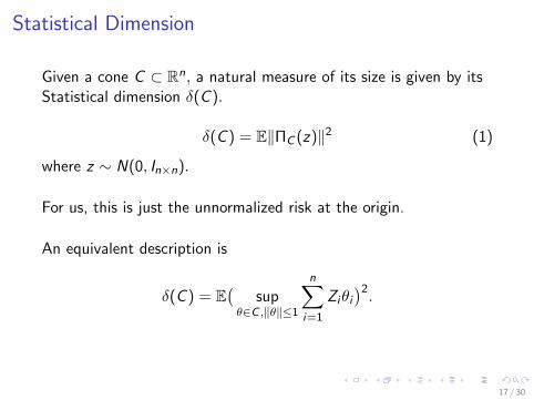
Statistical Dimension

Given a cone C ⊂ Rn, a natural measure of its size is given by itsStatistical dimension δ(C ).

δ(C ) = E‖ΠC (z)‖2 (1)

where z ∼ N(0, In×n).

For us, this is just the unnormalized risk at the origin.

An equivalent description is

δ(C ) = E(

supθ∈C ,‖θ‖≤1

n∑i=1

Ziθi)2.

17 / 30

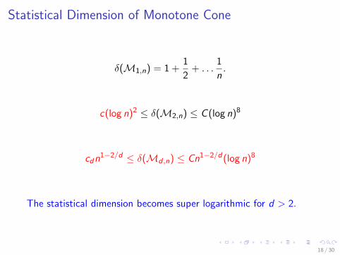
Statistical Dimension of Monotone Cone

δ(M1,n) = 1 +1

2+ . . .

1

n.

c(log n)2 ≤ δ(M2,n) ≤ C (log n)8

cdn1−2/d ≤ δ(Md ,n) ≤ Cn1−2/d(log n)8

The statistical dimension becomes super logarithmic for d > 2.

18 / 30

Proof Ideas

To prove the upper bounds for d ≥ 3, it is useful to view thelattice Ld ,n as a collection of kd−2 = n(d−2)/d many twodimensional lattices.

Enlarge Md ,n by removing the constraints between the lattices.Then an upper bound to δ(Md ,n) is just the sum of δ(M2,n2/d )times the number of two dimensional lattices.

To prove the lower bound we make the Gaussian supremum innerproduct large by setting the values to be proportional to theGaussian vector on the antichain.

19 / 30

ADAPTATION OF THE LSE

20 / 30

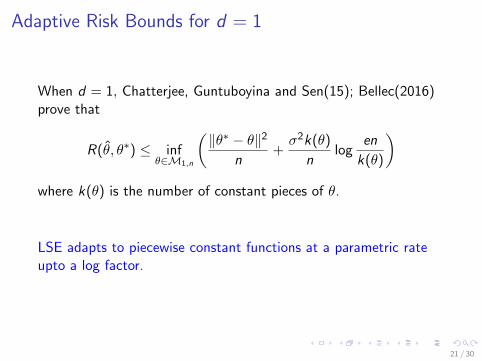
Adaptive Risk Bounds for d = 1

When d = 1, Chatterjee, Guntuboyina and Sen(15); Bellec(2016)prove that

R(θ, θ∗) ≤ infθ∈M1,n

(‖θ∗ − θ‖2

n+σ2k(θ)

nlog

en

k(θ)

)where k(θ) is the number of constant pieces of θ.

LSE adapts to piecewise constant functions at a parametric rateupto a log factor.

21 / 30

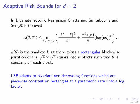
Adaptive Risk Bounds for d = 2

In Bivariate Isotonic Regression Chatterjee, Guntuboyina andSen(2016) proved

R(θ, θ∗) ≤ infθ∈M2,n

(‖θ∗ − θ‖2

n+σ2k(θ)

n(log(en))8

).

k(θ) is the smallest k s.t there exists a rectangular block-wisepartition of the

√n ×√n square into k blocks such that θ is

constant on each block.

LSE adapts to bivariate non decreasing functions which arepiecewise constant on rectangles at a parametric rate upto a logfactor.

22 / 30

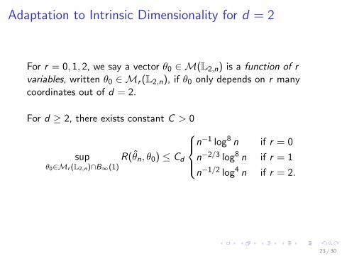
Adaptation to Intrinsic Dimensionality for d = 2

For r = 0, 1, 2, we say a vector θ0 ∈M(L2,n) is a function of rvariables, written θ0 ∈Mr (L2,n), if θ0 only depends on r manycoordinates out of d = 2.

For d ≥ 2, there exists constant C > 0

supθ0∈Mr (L2,n)∩B∞(1)

R(θn, θ0) ≤ Cd

n−1 log8 n if r = 0

n−2/3 log8 n if r = 1

n−1/2 log4 n if r = 2.

23 / 30

Adaptive Risk Bound for d > 2?

The LSE has a O(n−2/d) rate of convergence when θ∗ is aconstant function; parametric adaptation therefore is not possible.

However this rate is faster than the minimax rate of convergenceO(n−1/d).

It is still natural to surmise that the LSE will have faster rate ofconvergence than the minimax rate whenever θ∗ is piecewise

constant on rectangles; subsets of the lattice of the formd∏

i=1

[ai , bi ].

24 / 30

Adaptive Risk Bound for d > 2?

It is useful to view the lattice Ld ,n as a collection of twodimensional lattices; for example by fixing d − 2 coordinates.

One can then apply the existing adaptation result for 2 dimensionallattices in Chatterjee, Guntuboyina, Sen(2016) on each of theselattices.

25 / 30

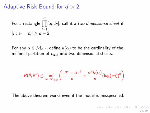
Adaptive Risk Bound for d > 2

For a rectangled∏

i=1

[ai , bi ], call it a two dimensional sheet if

|i : ai = bi | ≥ d − 2.

For any α ∈Md ,n, define k(α) to be the cardinality of theminimal partition of Ld ,n into two dimensional sheets.

R(θ, θ∗) ≤ infα∈Md,n

(‖θ∗ − α‖2

n+σ2k(α)

n(log(en))8

).

The above theorem works even if the model is misspecified.

26 / 30

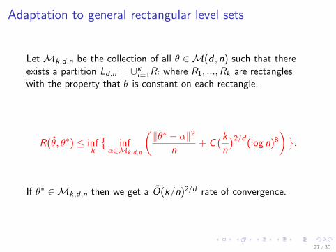
Adaptation to general rectangular level sets

Let Mk,d ,n be the collection of all θ ∈M(d , n) such that thereexists a partition Ld ,n = ∪ki=1Ri where R1, ...,Rk are rectangleswith the property that θ is constant on each rectangle.

R(θ, θ∗) ≤ infk

{inf

α∈Mk,d,n

(‖θ∗ − α‖2

n+ C

(kn

)2/d(log n)8

)}.

If θ∗ ∈Mk,d ,n then we get a O(k/n)2/d rate of convergence.

27 / 30

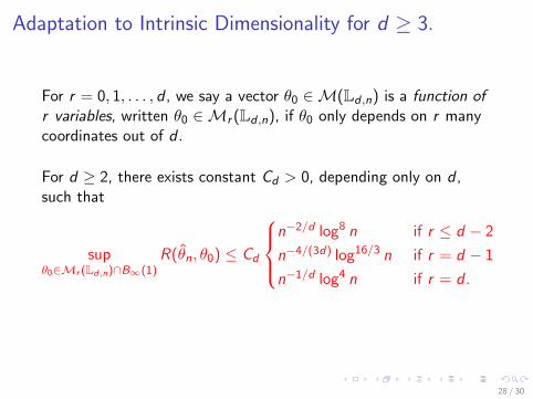
Adaptation to Intrinsic Dimensionality for d ≥ 3.

For r = 0, 1, . . . , d , we say a vector θ0 ∈M(Ld ,n) is a function ofr variables, written θ0 ∈Mr (Ld ,n), if θ0 only depends on r manycoordinates out of d .

For d ≥ 2, there exists constant Cd > 0, depending only on d ,such that

supθ0∈Mr (Ld,n)∩B∞(1)

R(θn, θ0) ≤ Cd

n−2/d log8 n if r ≤ d − 2

n−4/(3d) log16/3 n if r = d − 1

n−1/d log4 n if r = d .

28 / 30

Summary

LSE is minimax rate optimal with O(n−1/d) rate of convergence.

The Statistical Dimension of the Monotone Cone becomes superlogarithmic as soon as d > 2.

Nearly parametric adaptation to piecewise constant functions is nolonger obtained as in d = 1 and 2 but faster rates than theminimax rates are still obtained when θ∗ has additional structuresuch as piecewise constant on rectangles or when intrinsicdimensionality is lower than d .

29 / 30

THANK YOU!

30 / 30