Algorithms and Applications in Social Networks

2021/2022, Semester A

Slava Novgorodov 1

Lesson #2

• Random network models

• Centrality measures

2

Random Graphs

3

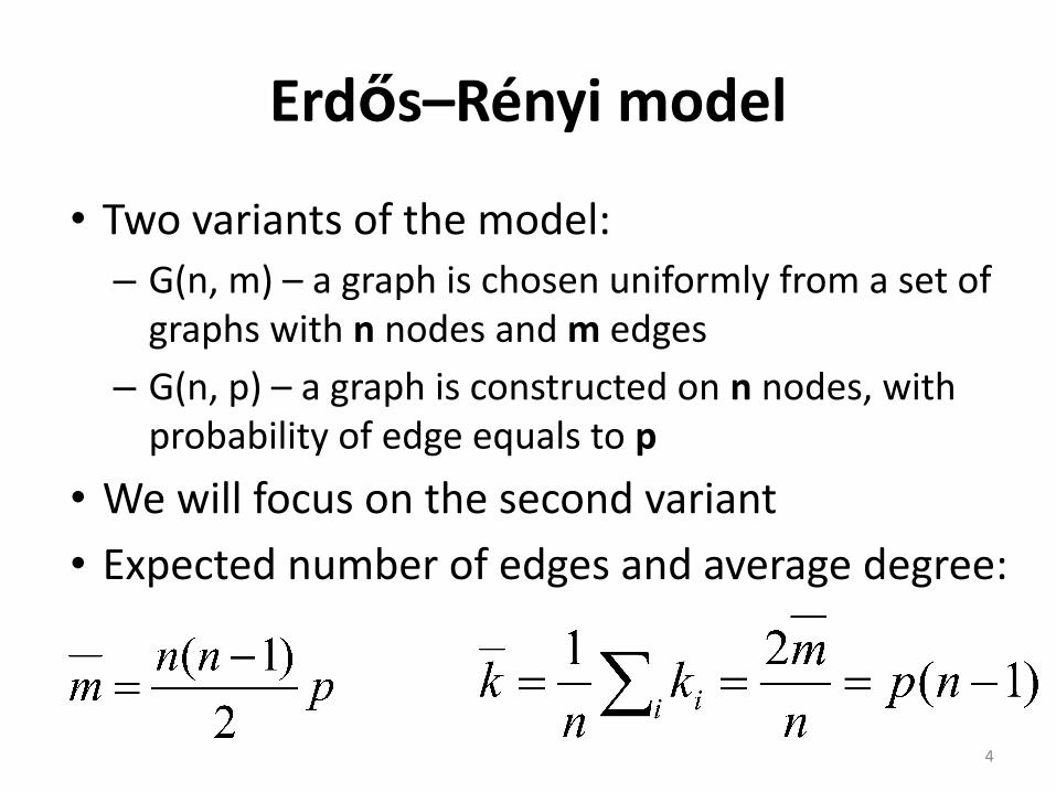
Erdős–Rényi model

• Two variants of the model:– G(n, m) – a graph is chosen uniformly from a set of

graphs with n nodes and m edges

– G(n, p) – a graph is constructed on n nodes, with probability of edge equals to p

• We will focus on the second variant

• Expected number of edges and average degree:

4

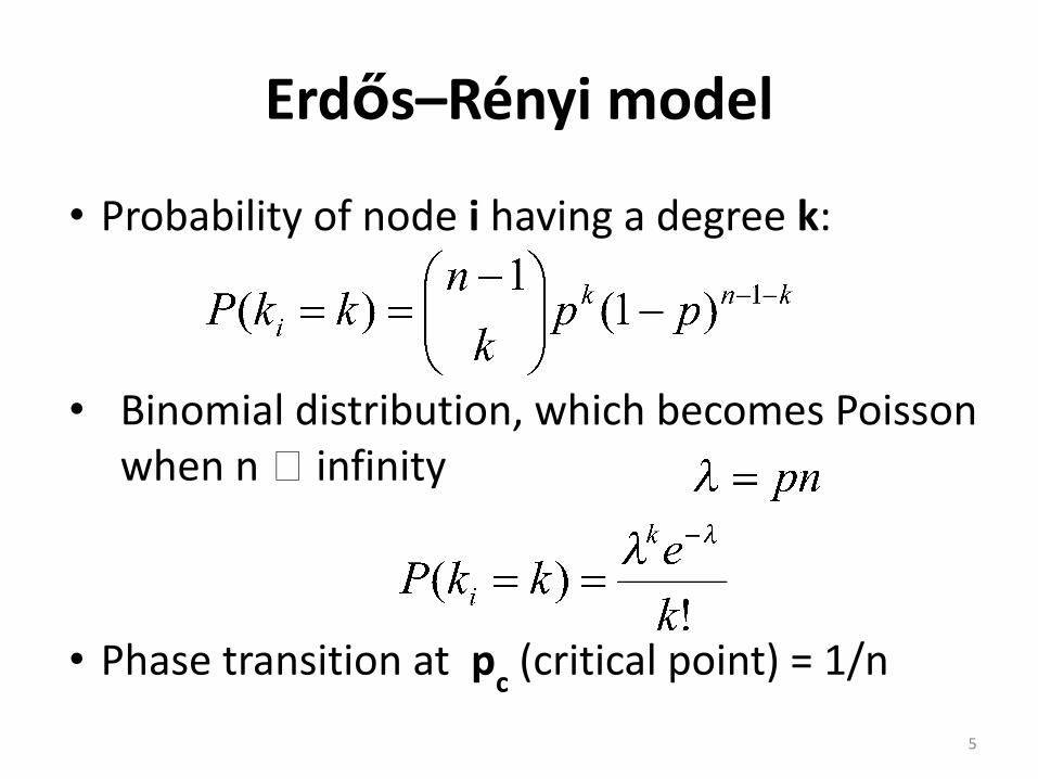
Erdős–Rényi model

• Probability of node i having a degree k:

• Binomial distribution, which becomes Poisson when n 🡪 infinity

• Phase transition at pc (critical point) = 1/n

5

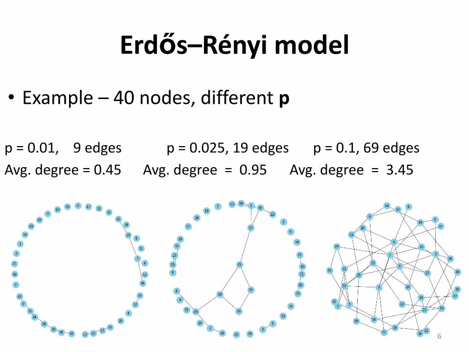
Erdős–Rényi model

• Example – 40 nodes, different p

p = 0.01, 9 edges p = 0.025, 19 edges p = 0.1, 69 edges

Avg. degree = 0.45 Avg. degree = 0.95 Avg. degree = 3.45

6

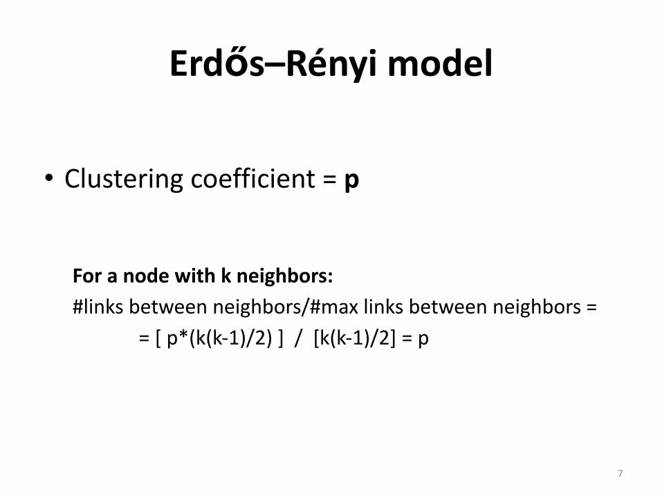
Erdős–Rényi model

• Clustering coefficient = p

For a node with k neighbors:

#links between neighbors/#max links between neighbors =

= [ p*(k(k-1)/2) ] / [k(k-1)/2] = p

7

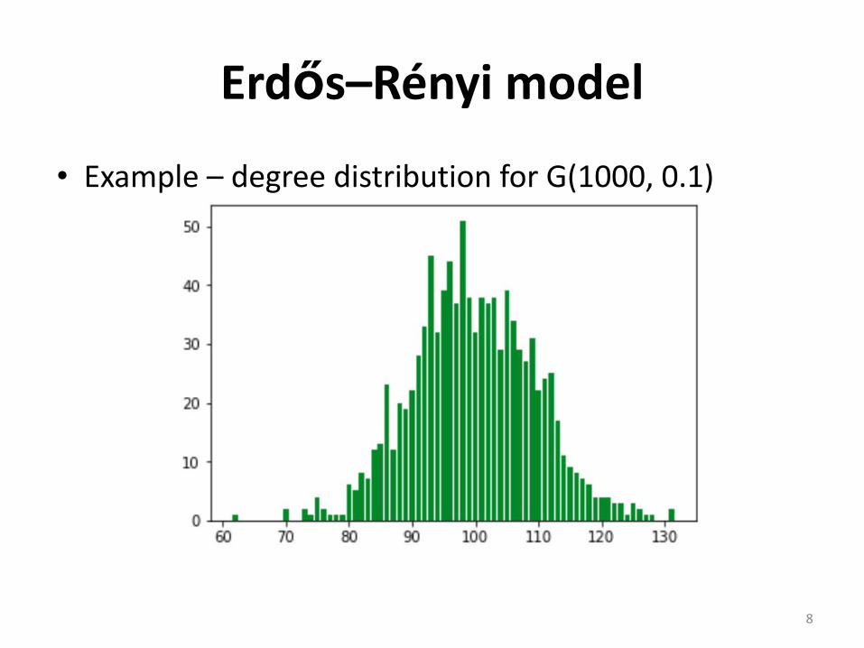
Erdős–Rényi model

• Example – degree distribution for G(1000, 0.1)

• Small diameter, but: (1) Non “power-law” distribution. (2) Low clustering coefficient. 🡪 Not a “small-world”

8

“Small-world” model

• Properties:– Small diameter (proportional to log N)

– High clustering coefficient

• A class of random graphs by Watts and Strogatz

9

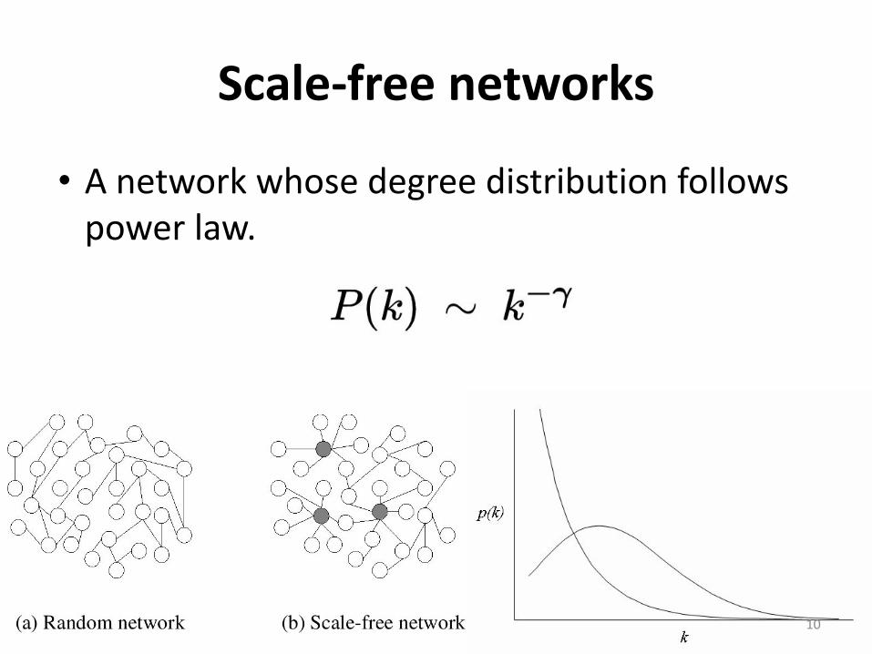
Scale-free networks

• A network whose degree distribution follows power law.

10

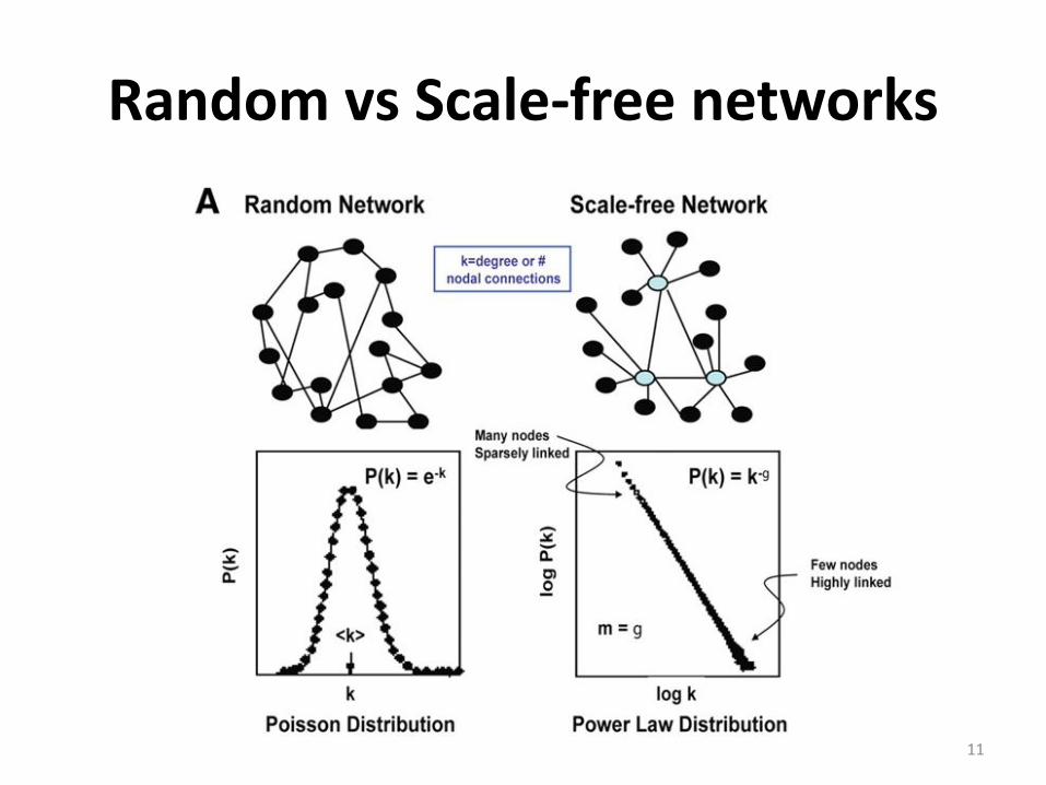
Random vs Scale-free networks

11

“Small-world” model

• Small-world examples:– Co-authors in the same domain

– Colleagues

– Classmates

• Non small-world examples:– “went-to-same-school” people

12

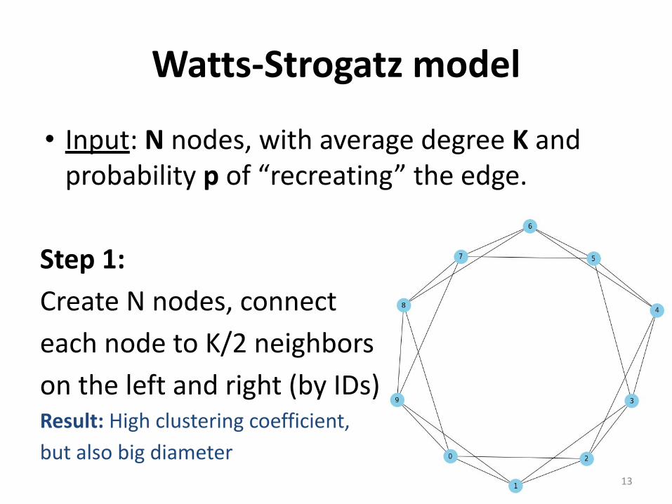
Watts-Strogatz model

• Input: N nodes, with average degree K and probability p of “recreating” the edge.

Step 1:

Create N nodes, connect

each node to K/2 neighbors

on the left and right (by IDs)Result: High clustering coefficient,

but also big diameter 13

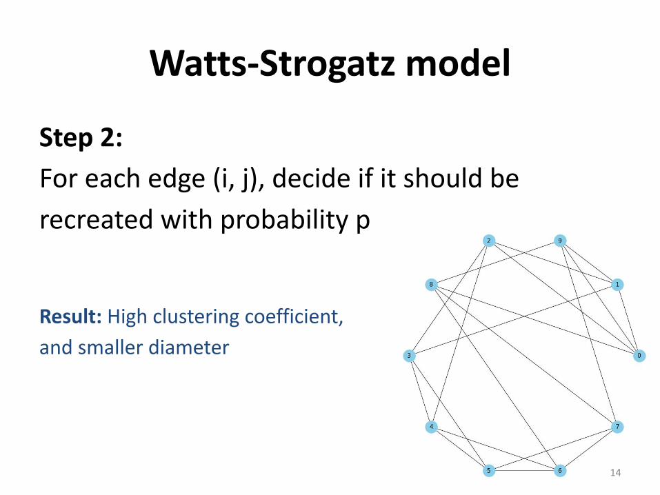
Watts-Strogatz model

Step 2:

For each edge (i, j), decide if it should be

recreated with probability p

Result: High clustering coefficient,

and smaller diameter

14

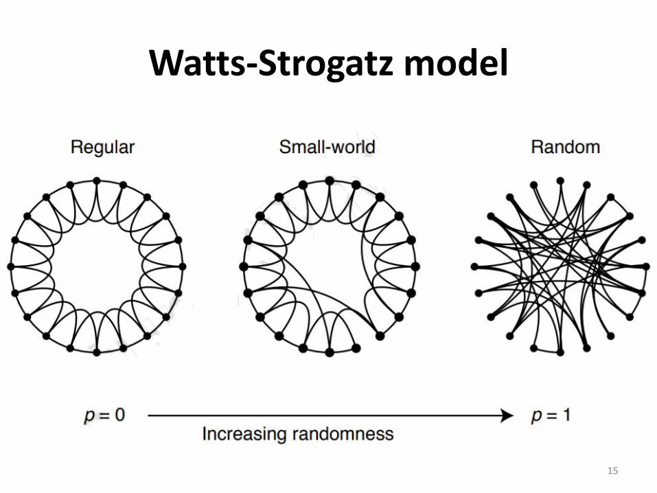
Watts-Strogatz model

15

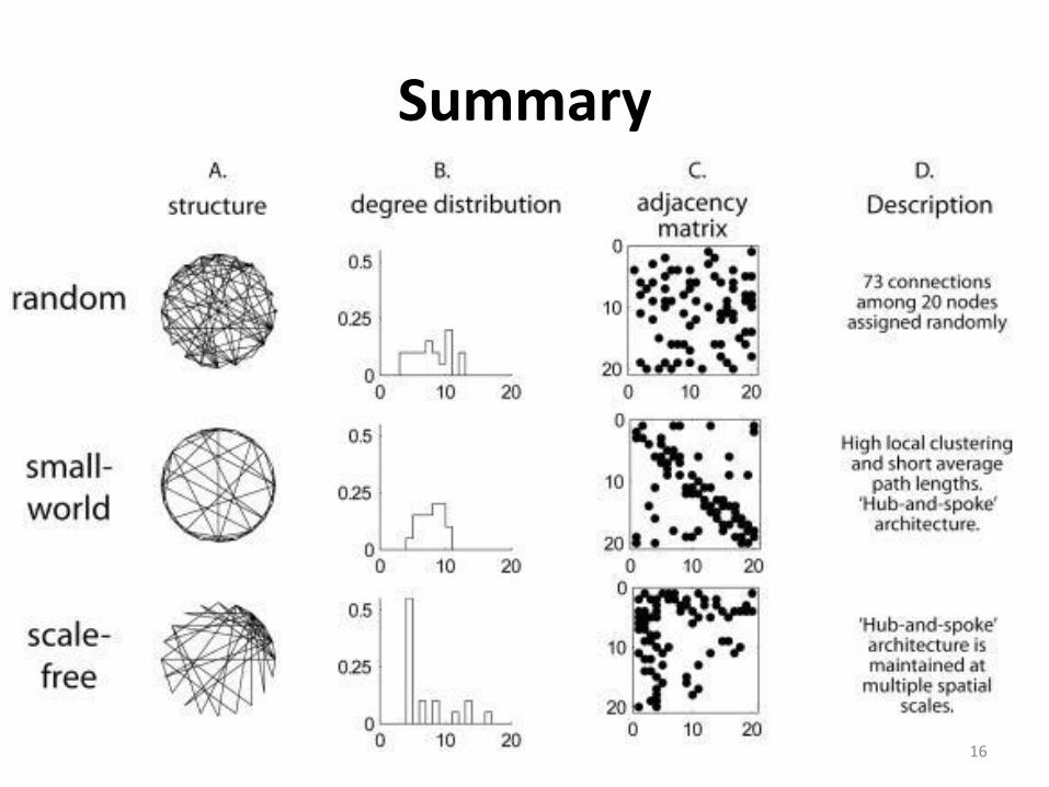
Summary

16

Real World examples

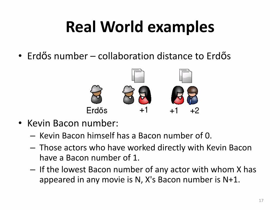
• Erdős number – collaboration distance to Erdős

• Kevin Bacon number:– Kevin Bacon himself has a Bacon number of 0.– Those actors who have worked directly with Kevin Bacon

have a Bacon number of 1.– If the lowest Bacon number of any actor with whom X has

appeared in any movie is N, X's Bacon number is N+1.

17

Erdős–Bacon number

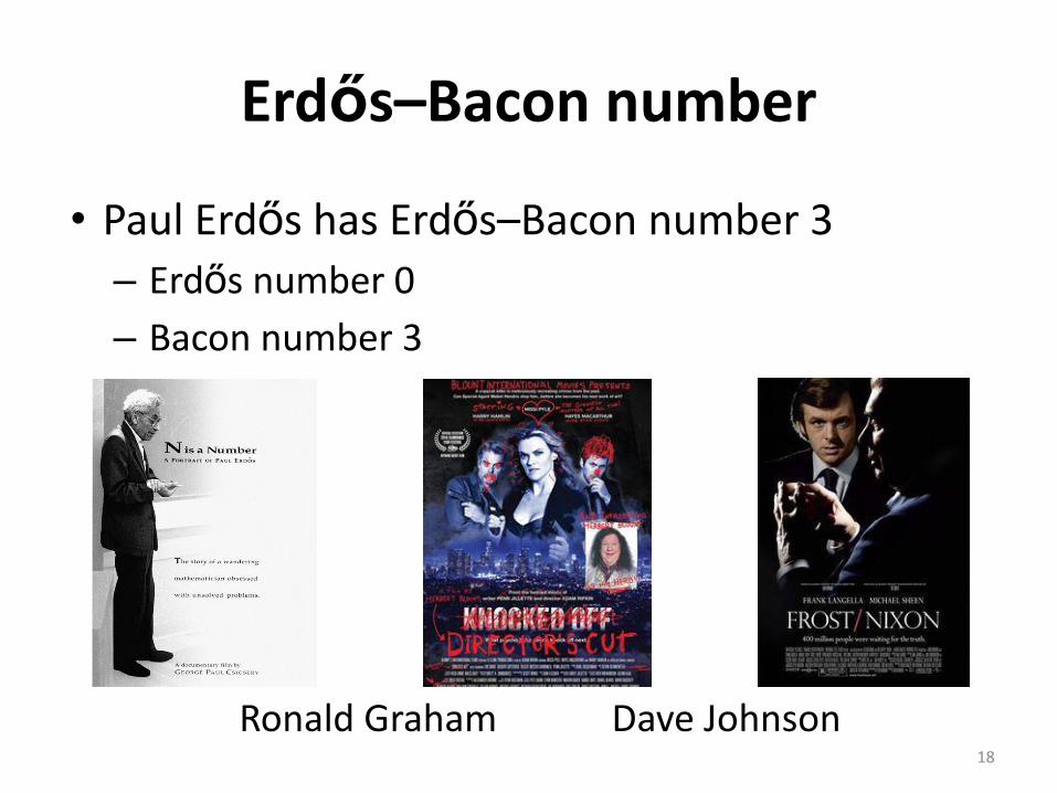
• Paul Erdős has Erdős–Bacon number 3– Erdős number 0

– Bacon number 3

Ronald Graham Dave Johnson18

Erdős–Bacon number

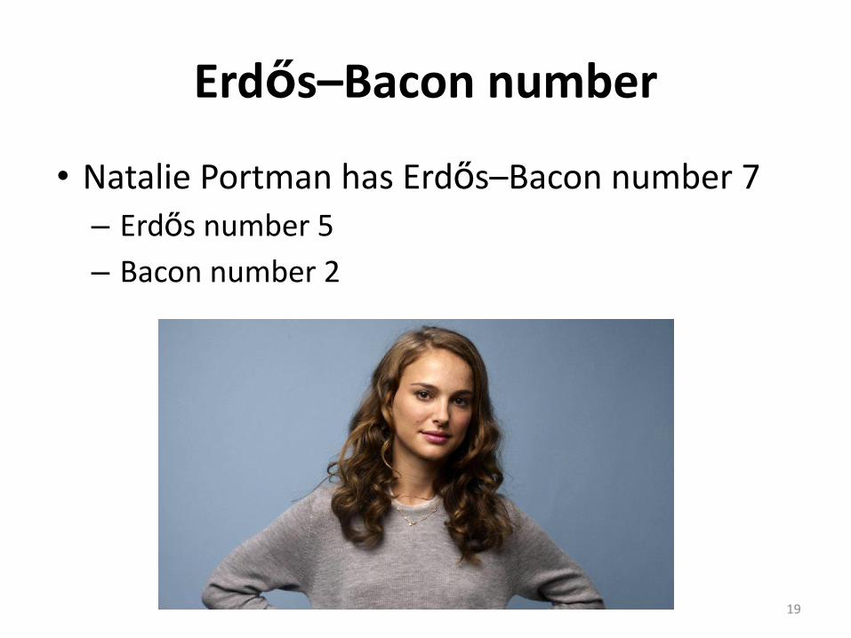
• Natalie Portman has Erdős–Bacon number 7– Erdős number 5

– Bacon number 2

19

Centrality Measures

20

Centrality

• Identify the most important vertices in a graph

• Applications:– Most influential people

– Key infrastructure nodes

– Information spread points

• The measure we chose is often depends on the application

21

Preliminaries

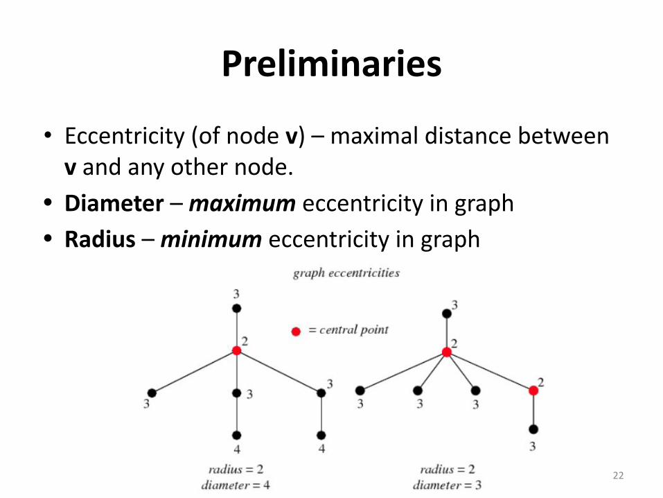
• Eccentricity (of node v) – maximal distance between v and any other node.

• Diameter – maximum eccentricity in graph

• Radius – minimum eccentricity in graph

22

Preliminaries

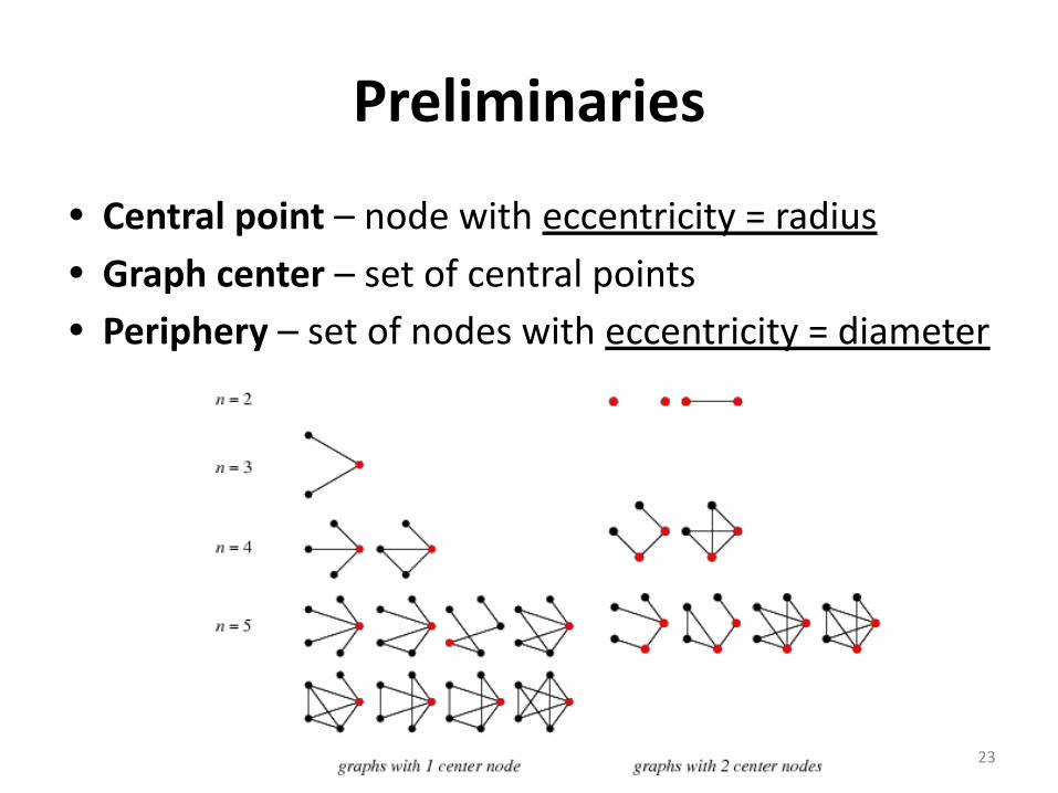
• Central point – node with eccentricity = radius

• Graph center – set of central points

• Periphery – set of nodes with eccentricity = diameter

23

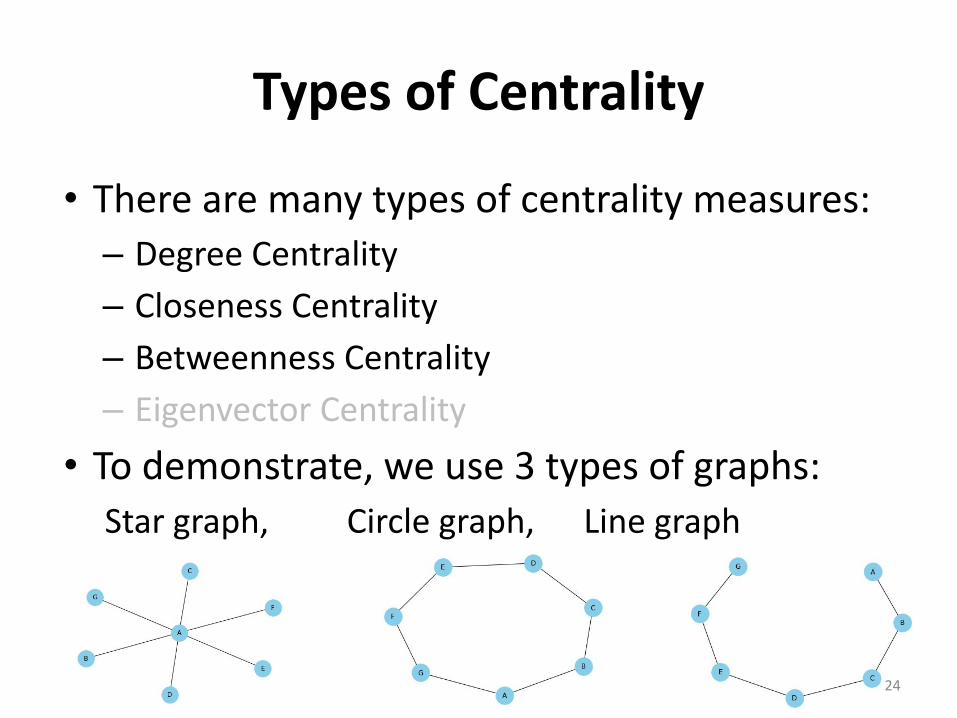
Types of Centrality

• There are many types of centrality measures:– Degree Centrality

– Closeness Centrality

– Betweenness Centrality

– Eigenvector Centrality

• To demonstrate, we use 3 types of graphs:Star graph, Circle graph, Line graph

24

Things to measure

• Degree Centrality:– Connectedness

• Closeness Centrality:– Ease of reaching other nodes

• Betweenness Centrality:– Role as an intermediary, connector

• Eigenvector Centrality– “Whom you know…”

25

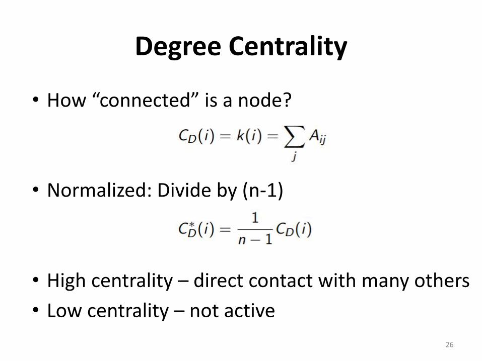
Degree Centrality

• How “connected” is a node?

• Normalized: Divide by (n-1)

• High centrality – direct contact with many others

• Low centrality – not active

26

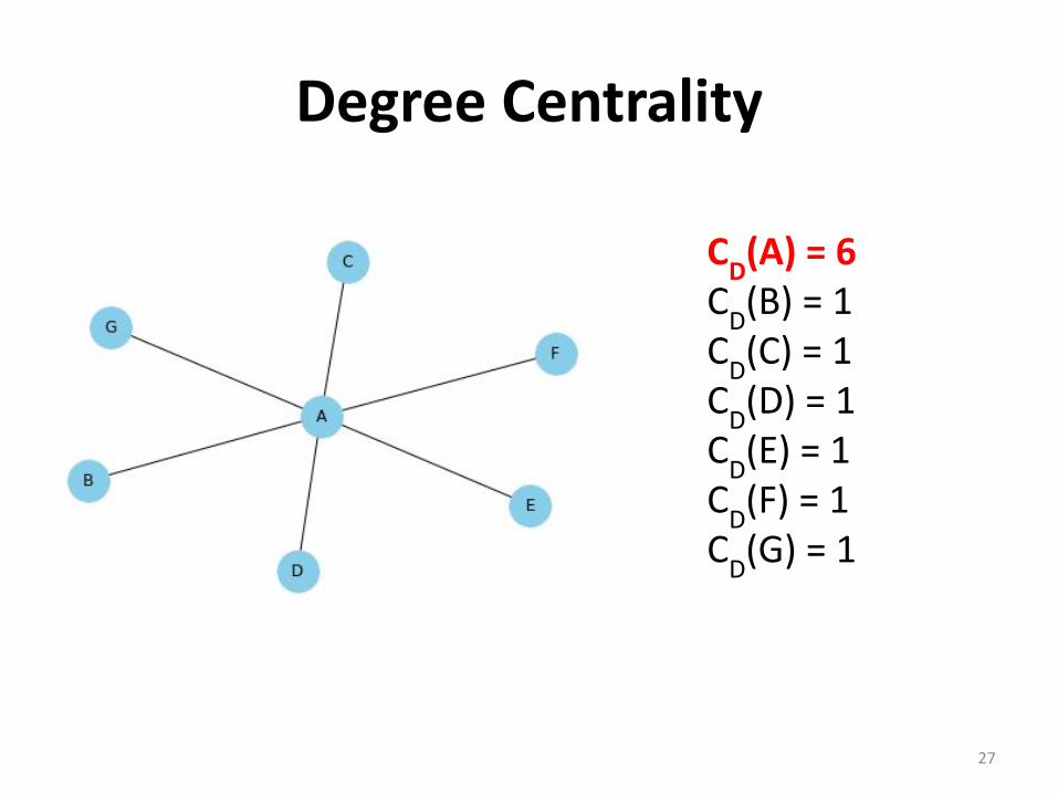
Degree Centrality

CD(A) = 6

CD(B) = 1

CD(C) = 1

CD(D) = 1

CD(E) = 1

CD(F) = 1

CD(G) = 1

27

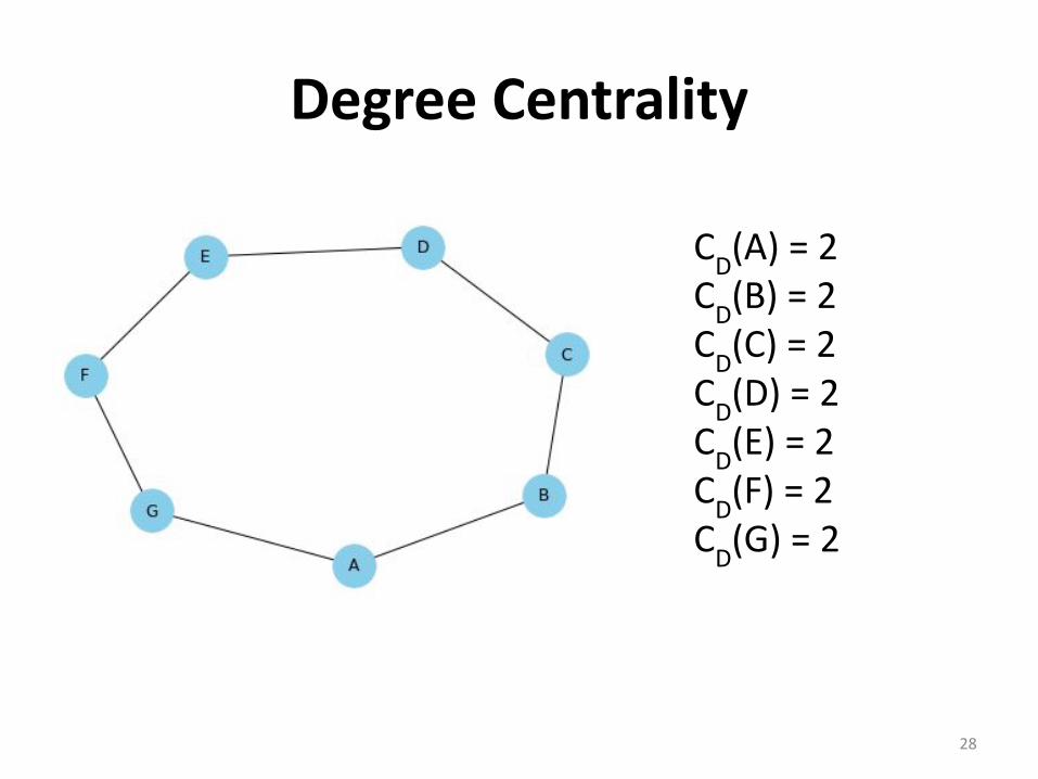
Degree Centrality

CD(A) = 2

CD(B) = 2

CD(C) = 2

CD(D) = 2

CD(E) = 2

CD(F) = 2

CD(G) = 2

28

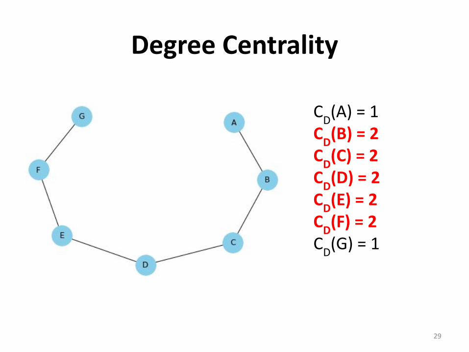
Degree Centrality

CD(A) = 1

CD(B) = 2

CD(C) = 2

CD(D) = 2

CD(E) = 2

CD(F) = 2

CD(G) = 1

29

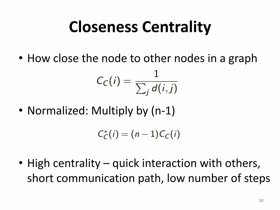
Closeness Centrality

• How close the node to other nodes in a graph

• Normalized: Multiply by (n-1)

• High centrality – quick interaction with others, short communication path, low number of steps

30

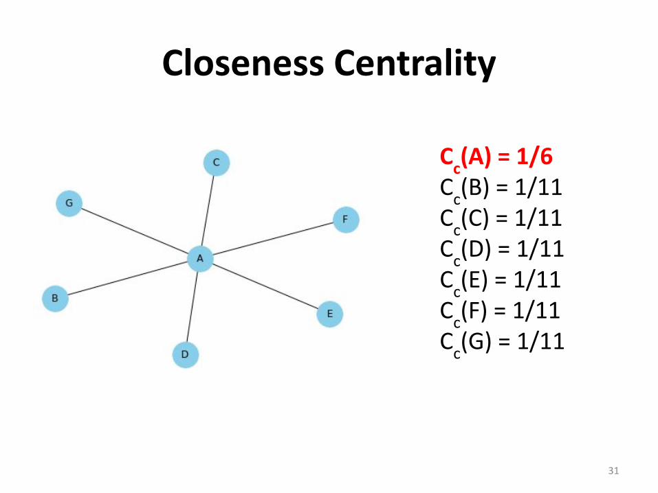
Closeness Centrality

Cc(A) = 1/6

Cc(B) = 1/11

Cc(C) = 1/11

Cc(D) = 1/11

Cc(E) = 1/11

Cc(F) = 1/11

Cc(G) = 1/11

31

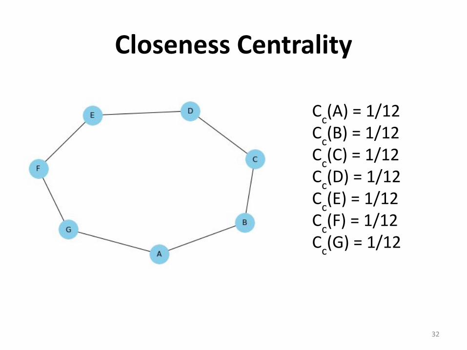
Closeness Centrality

Cc(A) = 1/12

Cc(B) = 1/12

Cc(C) = 1/12

Cc(D) = 1/12

Cc(E) = 1/12

Cc(F) = 1/12

Cc(G) = 1/12

32

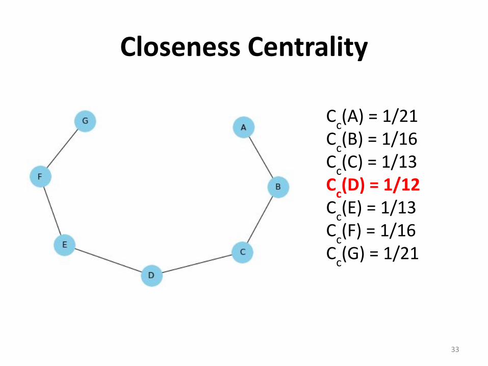
Closeness Centrality

Cc(A) = 1/21

Cc(B) = 1/16

Cc(C) = 1/13

Cc(D) = 1/12

Cc(E) = 1/13

Cc(F) = 1/16

Cc(G) = 1/21

33

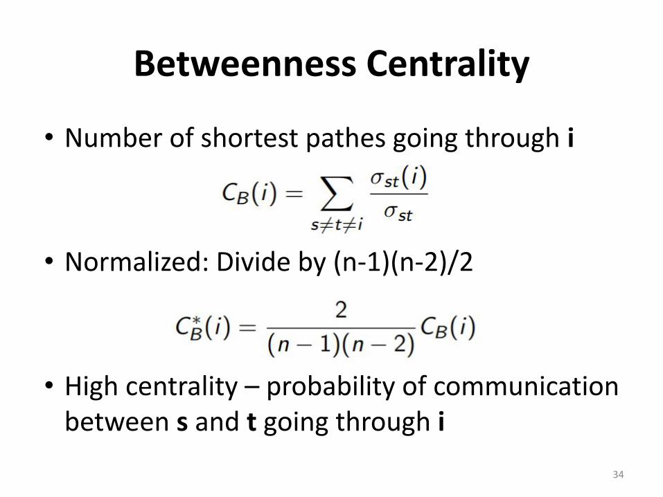
Betweenness Centrality

• Number of shortest pathes going through i

• Normalized: Divide by (n-1)(n-2)/2

• High centrality – probability of communication between s and t going through i

34

Betweenness Centrality

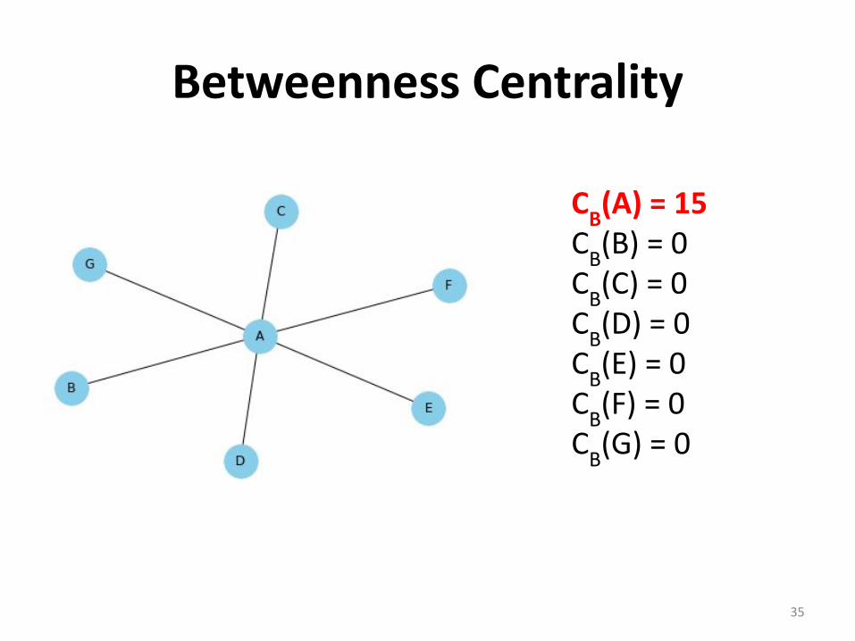
CB(A) = 15

CB(B) = 0

CB(C) = 0

CB(D) = 0

CB(E) = 0

CB(F) = 0

CB(G) = 0

35

Betweenness Centrality

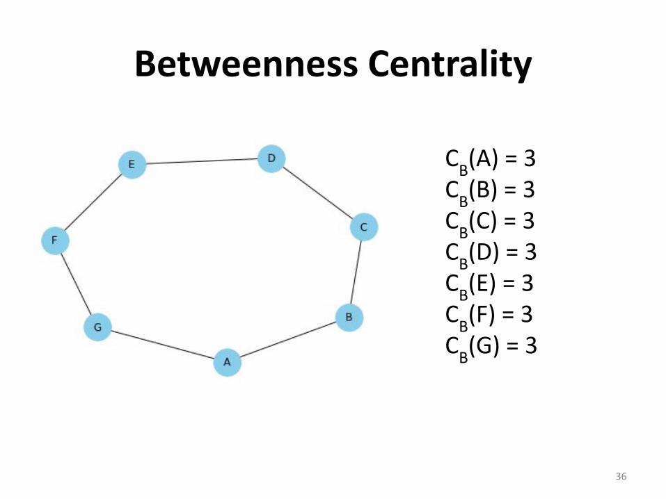
CB(A) = 3

CB(B) = 3

CB(C) = 3

CB(D) = 3

CB(E) = 3

CB(F) = 3

CB(G) = 3

36

Betweenness Centrality

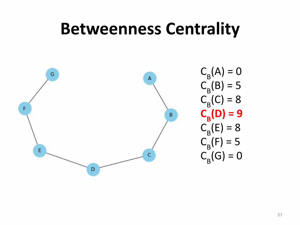
CB(A) = 0

CB(B) = 5

CB(C) = 8

CB(D) = 9

CB(E) = 8

CB(F) = 5

CB(G) = 0

37

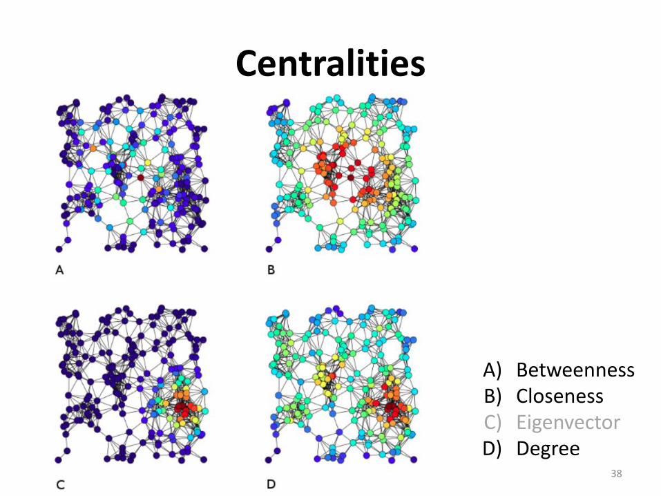
Centralities

A) BetweennessB) ClosenessC) EigenvectorD) Degree

38

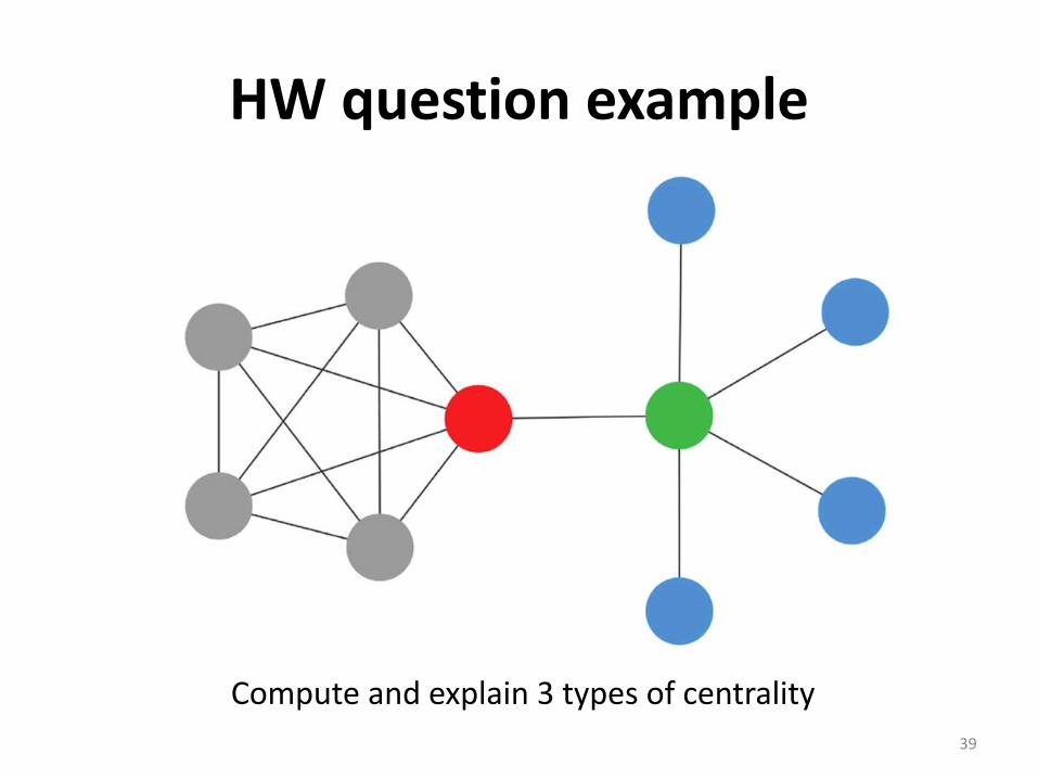
HW question example

Compute and explain 3 types of centrality

39

Families of Florence

• Marriage and relationships of 16 families in Florence in middle ages

• Very interesting, “classic” network to analyze

• The rise of Medici family (https://www2.bc.edu/candace-jones/mb851/Mar12/PadgettAnsell_AJS_1993.pdf)

40

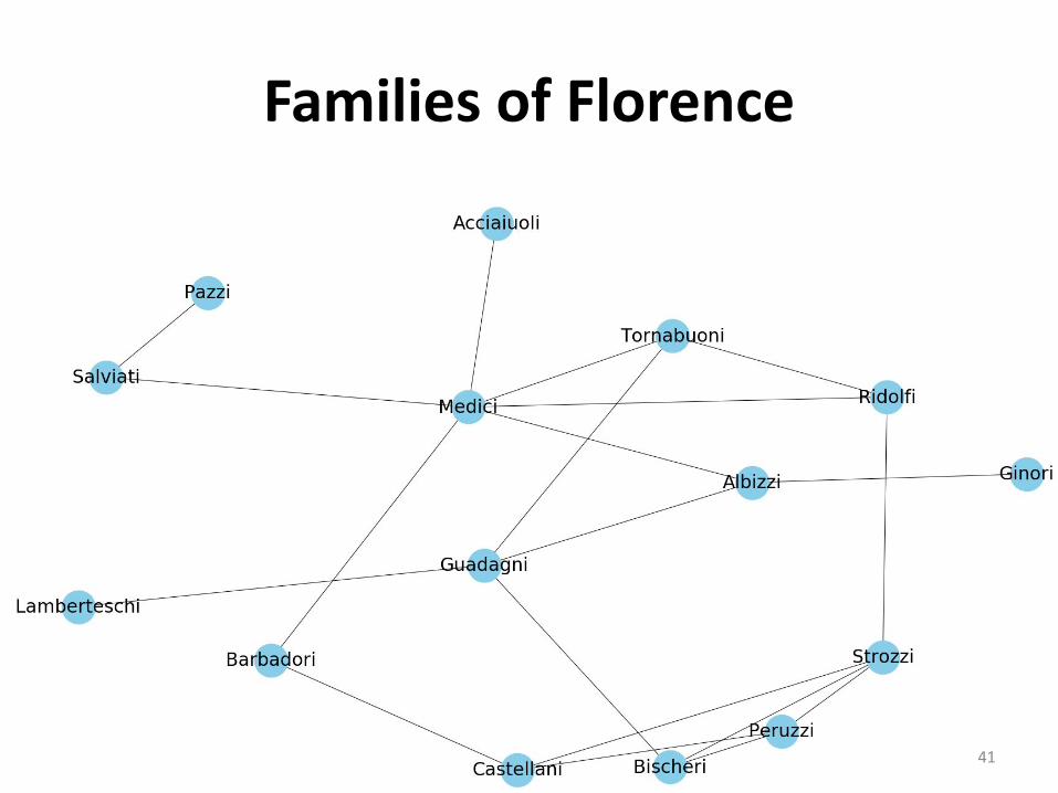
Families of Florence

41

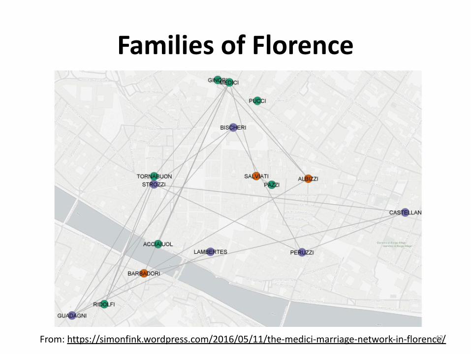
Families of Florence

From: https://simonfink.wordpress.com/2016/05/11/the-medici-marriage-network-in-florence/42

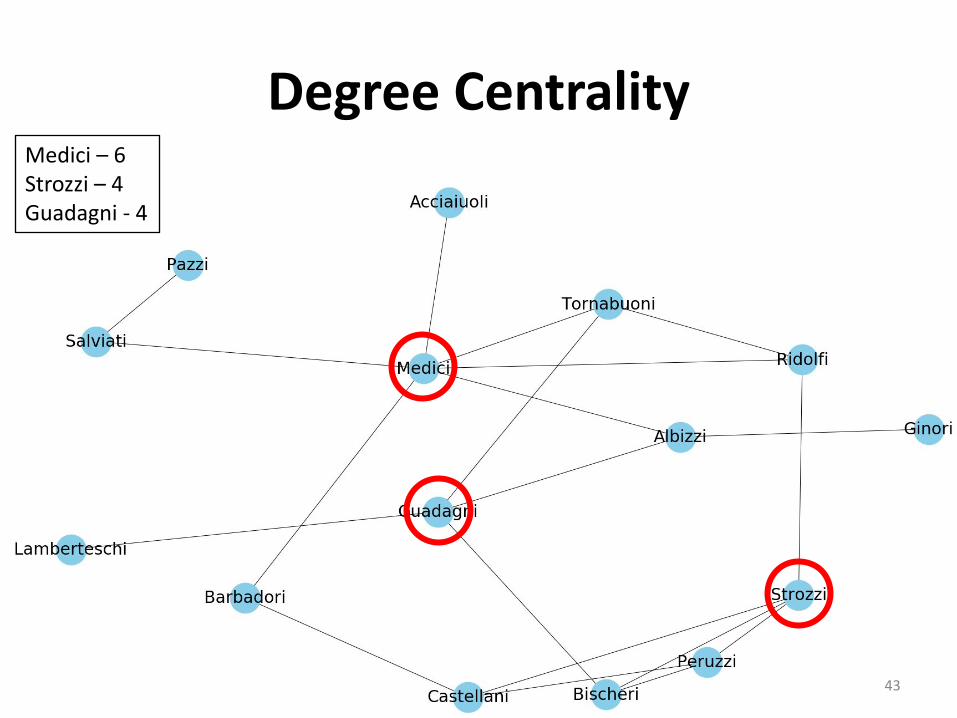
Degree CentralityMedici – 6Strozzi – 4Guadagni - 4

43

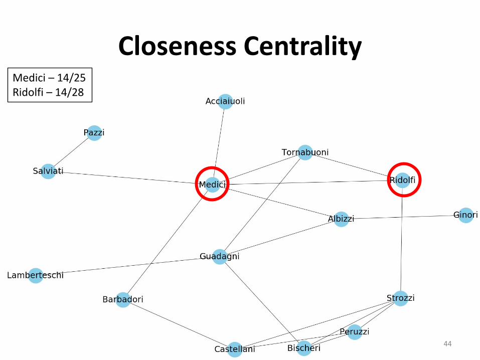
Closeness CentralityMedici – 14/25Ridolfi – 14/28

44

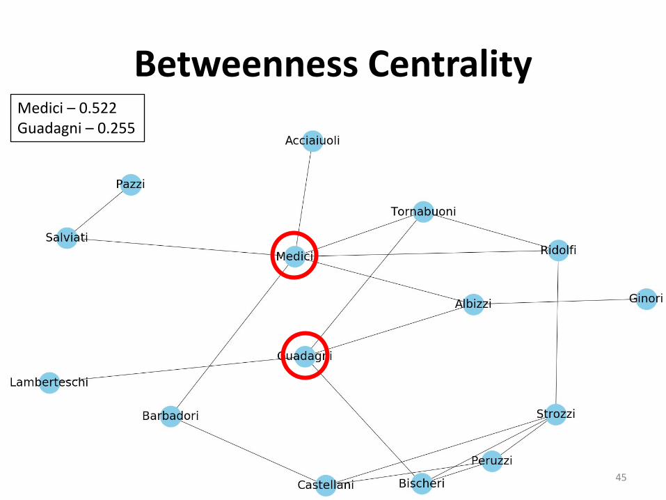
Betweenness CentralityMedici – 0.522Guadagni – 0.255

45

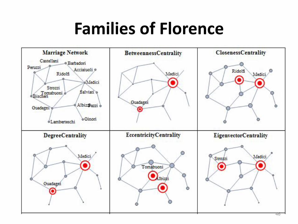
Families of Florence

46

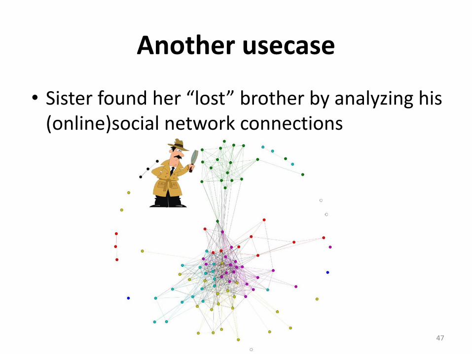
Another usecase

• Sister found her “lost” brother by analyzing his (online)social network connections

47

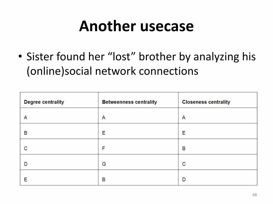
Another usecase

• Sister found her “lost” brother by analyzing his (online)social network connections

48

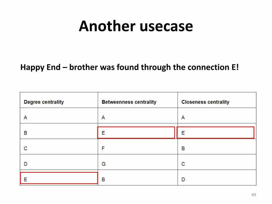
Another usecase

Happy End – brother was found through the connection E!

49

Thank you!Questions?

50