Embed Size (px)
Citation preview

Characterisation and Applications of MANET
Routing Algorithms in Wireless Sensor
Networks
Siddhu Warrier
TH
E
U N I V E RS
IT
Y
OF
ED I N B U
RG
H
Master of Science
School of Informatics
University of Edinburgh
2007
Abstract
Wireless Sensor Networks (WSN) are networks of low-cost, low-power, multi-
functional devices that can be used to monitor physical phenomena. Communication
between nodes in a vast network requires routing mechanisms. A Specknet is a pro-
grammable computational network of large numbers of minute semiconductor compo-
nents with integrated sensing, processing and wireless networking capabilities called
Specks.
This thesis sets to analyse the feasibility of using Mobile Ad-hoc Network (MANET)
routing mechanisms in Wireless Sensor Networks, and to investigate application do-
mains where MANET algorithms can be used. Therefore, the Destination Sequenced
Distance Vector (DSDV) and Zone Routing Protocol (ZRP) algorithms, and a Visitor
Tracking System (VTS) application using the DSDV algorithm were implemented on
prototypes of Specks called the ProSpeckz.
The suitability of the algorithms and the performance of the application are anal-
ysed using several experiments. The results of the experiments indicate that MANET
algorithms such as the DSDV algorithm are candidates for use in certain WSN appli-
cations. It is also learnt that the DSDV algorithm, while more responsive when used in
small networks, is less scalable than the ZRP algorithm.
Future work includes improving the performance of the implementations analysed
by performing optimisations to MAC algorithm characteristics and additions to net-
work layer functionality, and extending the ZRP algorithm to new application domains.
i
AcknowledgementsFirst and foremost, I would like to thank my supervisor, Dr. D.K. Arvind, Reader,
School of Informatics, University of Edinburgh, for his constant guidance, and for
having provided me both material and moral support over an extremely staggered thesis
timetable.
I would like to thank Prof. Klaus Wehrle, Head, Distributed Systems Group, Chair
of Computer Science IV, RWTH Aachen, for consenting to be my second supervisor,
and for agreeing to mark my thesis at an extremely short notice.
Just as importantly, my thanks go out to Dr. Steven K.J. Wong, Nanyang Tech-
nological University, Singapore, who helped me get started, wrote the SpeckMAC
algorithm, and helped immeasurably in the implementation of the DSDV algorithm.
I would also like to thank the European Commission for funding me over the past
two years, as well as Agilent Technologies, who funded me during a part of this work.
This section would be incomplete if I failed to acknowledge Mat Barnes, Research
Associate, School of Informatics, University of Edinburgh, for guiding me millions of
times when I was stuck, sitting through long debugging sessions of my (often un-
sightly) code, helping me with hardware problems, and reading my thesis.
I would also like to express my gratitude to my good friend Mohammad Dmour,
who has very patiently proof-read this work.
I would like to express my heartfelt gratitude to Alex Young and Martin Ling,
School of Informatics, University of Edinburgh, for having patiently explained certain
concepts to me, taught me to use some of the equipment in the lab, and for having
steered me through choppy waters.
Tom Feist, who designed the foundation upon which part of this work is based
on, also deserves my sincere thanks, as do Ryan Mc Nally and Janek Mann, School
of Informatics, University of Edinburgh, for having suggested tracking mechanisms to
investigate.
Dipl. Inf. Jo Agila Bitsch Link, Chair of Computer Science IV, RWTH Aachen,
deserves my gratitude for having proof-read my thesis and provided me with detailed
feedback, as does Galiia Khasanova for having taken a look at my thesis and for
having tolerated me and my endless rants for as long as she has.
Last but definitely not the least, I would like to thank my parents for, well, being
loving parents and for having resisted the wholly understandable temptation to drown
me when I was still an (insufferable) child. Society probably suffers from that decision
of theirs borne out of parental love, but I sure got lucky!
ii

Declaration
I declare that this thesis was composed by myself, that the work contained herein is
my own except where explicitly stated otherwise in the text, and that this work has not
been submitted for any other degree or professional qualification except as specified.
( Siddhu Warrier
iii

This thesis is dedicated to Eric Cartman, Southpark, Colorado, USA, for his
unflinching guidance, and for having shaped my philosophy in life.
iv
Table of Contents
1 Introduction 11.1 Rationale . . . . . . . . . . . . . . . . . . . . . . . . . . . . . . . . 1
1.2 Algorithm Characterisation . . . . . . . . . . . . . . . . . . . . . . . 2
1.3 Applications . . . . . . . . . . . . . . . . . . . . . . . . . . . . . . . 3
1.3.1 Visitor Tracking System . . . . . . . . . . . . . . . . . . . . 3
1.4 Outline . . . . . . . . . . . . . . . . . . . . . . . . . . . . . . . . . 4
2 Background 52.1 Wireless Sensor Networks . . . . . . . . . . . . . . . . . . . . . . . 5
2.1.1 Architecture and constraints . . . . . . . . . . . . . . . . . . 6
2.1.2 Deployment Structure and Topology . . . . . . . . . . . . . . 7
2.1.3 Protocol Stack on a typical Sensor Node . . . . . . . . . . . . 7
2.2 Specknets and the ProSpeckz IIK . . . . . . . . . . . . . . . . . . . . 8
2.2.1 Overview . . . . . . . . . . . . . . . . . . . . . . . . . . . . 9
2.2.2 The Prospeckz IIK . . . . . . . . . . . . . . . . . . . . . . . 9
2.3 The MAC Layer in Wireless Sensor Networks . . . . . . . . . . . . . 11
2.4 SpeckMAC . . . . . . . . . . . . . . . . . . . . . . . . . . . . . . . 12
2.4.1 SpeckMAC-B . . . . . . . . . . . . . . . . . . . . . . . . . . 13
2.4.2 SpeckMAC-D . . . . . . . . . . . . . . . . . . . . . . . . . . 14
2.4.3 Why SpeckMAC? . . . . . . . . . . . . . . . . . . . . . . . 14
2.5 Routing in Wireless Sensor Networks . . . . . . . . . . . . . . . . . 15
2.5.1 Classification of routing protocols . . . . . . . . . . . . . . . 16
2.5.2 Classification of WSN routing protocols . . . . . . . . . . . . 16
2.6 Destination-Sequenced Distance-Vector Routing (DSDV) . . . . . . . 17
2.6.1 Distance Vector routing . . . . . . . . . . . . . . . . . . . . . 17
2.6.2 Sequence Numbers . . . . . . . . . . . . . . . . . . . . . . . 18
2.6.3 Broken Links . . . . . . . . . . . . . . . . . . . . . . . . . . 18
v
2.6.4 Full Routing Table Dump vs Incremental Routing Update . . 18
2.6.5 Preventing Routing Table Fluctuation . . . . . . . . . . . . . 19
2.6.6 Issues with the DSDV Algorithm . . . . . . . . . . . . . . . 19
2.7 Zone Routing Protocol . . . . . . . . . . . . . . . . . . . . . . . . . 19
2.7.1 Basic Operation . . . . . . . . . . . . . . . . . . . . . . . . . 20
2.7.2 Intra-zone communication in ZRP . . . . . . . . . . . . . . . 21
2.7.3 Inter-zone communication . . . . . . . . . . . . . . . . . . . 21
2.7.4 Properties of the ZRP routing algorithm . . . . . . . . . . . . 22
2.8 Tracking in WSNs . . . . . . . . . . . . . . . . . . . . . . . . . . . 22
2.9 Summary . . . . . . . . . . . . . . . . . . . . . . . . . . . . . . . . 23
3 Implementation of the DSDV Algorithm 253.1 Protocol Stack . . . . . . . . . . . . . . . . . . . . . . . . . . . . . . 25
3.2 Primitives and Data Structures . . . . . . . . . . . . . . . . . . . . . 26
3.2.1 MAC Layer Primitives . . . . . . . . . . . . . . . . . . . . . 26
3.2.2 Packet Types . . . . . . . . . . . . . . . . . . . . . . . . . . 29
3.2.3 The Routing Table . . . . . . . . . . . . . . . . . . . . . . . 31
3.3 Operational Example . . . . . . . . . . . . . . . . . . . . . . . . . . 35
3.3.1 Node Discovery and Route Propagation . . . . . . . . . . . . 38
3.3.2 Data Transmission . . . . . . . . . . . . . . . . . . . . . . . 41
3.3.3 Link Failure . . . . . . . . . . . . . . . . . . . . . . . . . . . 44
3.4 Summary . . . . . . . . . . . . . . . . . . . . . . . . . . . . . . . . 44
4 Applications using the DSDV Algorithm - Visitor Tracking System 454.1 Aim . . . . . . . . . . . . . . . . . . . . . . . . . . . . . . . . . . . 45
4.2 Requirements . . . . . . . . . . . . . . . . . . . . . . . . . . . . . . 46
4.3 Architecture . . . . . . . . . . . . . . . . . . . . . . . . . . . . . . . 46
4.3.1 Hardware and Software Platforms . . . . . . . . . . . . . . . 47
4.3.2 Protocol Stack . . . . . . . . . . . . . . . . . . . . . . . . . 47
4.3.3 The VTS in the Application Layer . . . . . . . . . . . . . . . 47
4.3.4 Packet Types in the Application Layer . . . . . . . . . . . . . 50
4.4 The VTS in operation . . . . . . . . . . . . . . . . . . . . . . . . . . 51
4.4.1 Stage 1 . . . . . . . . . . . . . . . . . . . . . . . . . . . . . 51
4.4.2 Stage 2 . . . . . . . . . . . . . . . . . . . . . . . . . . . . . 51
4.4.3 Stage 3 . . . . . . . . . . . . . . . . . . . . . . . . . . . . . 54
4.4.4 Stage 4 . . . . . . . . . . . . . . . . . . . . . . . . . . . . . 54
vi
4.5 Summary . . . . . . . . . . . . . . . . . . . . . . . . . . . . . . . . 55
5 Implementation of the ZRP Algorithm 565.1 Protocol Stack . . . . . . . . . . . . . . . . . . . . . . . . . . . . . . 56
5.2 Inter- and Intra-Zone communication . . . . . . . . . . . . . . . . . . 57
5.3 Modifications made to the DSDV implementation . . . . . . . . . . . 57
5.3.1 Changes to the DSDV implementation . . . . . . . . . . . . . 58
5.3.2 Code Optimisations and Additions . . . . . . . . . . . . . . . 58
5.4 Reactive Inter-Zone communication . . . . . . . . . . . . . . . . . . 58
5.4.1 Packet Types and the Inter-Zone Route Discovery Protocol . . 59
5.4.2 Route Caching Mechanisms . . . . . . . . . . . . . . . . . . 62
5.5 Operational Example . . . . . . . . . . . . . . . . . . . . . . . . . . 62
5.5.1 Stage 1 . . . . . . . . . . . . . . . . . . . . . . . . . . . . . 64
5.5.2 Stage 2 . . . . . . . . . . . . . . . . . . . . . . . . . . . . . 64
5.5.3 Stage 3 . . . . . . . . . . . . . . . . . . . . . . . . . . . . . 65
5.6 Summary . . . . . . . . . . . . . . . . . . . . . . . . . . . . . . . . 65
6 Experimental Methodology 666.1 Metrics Used for Characterisation . . . . . . . . . . . . . . . . . . . 66
6.1.1 Transmission Time . . . . . . . . . . . . . . . . . . . . . . . 67
6.1.2 Delivery Ratio . . . . . . . . . . . . . . . . . . . . . . . . . 67
6.1.3 Transmitter/Receiver On-time . . . . . . . . . . . . . . . . . 67
6.1.4 Metrics used for application characterisation . . . . . . . . . 68
6.2 Measurement Techniques . . . . . . . . . . . . . . . . . . . . . . . . 68
6.2.1 Measuring Transmission Latency . . . . . . . . . . . . . . . 69
6.2.2 Measuring Delivery Ratio . . . . . . . . . . . . . . . . . . . 73
6.2.3 Measuring Tx/Rx On-time . . . . . . . . . . . . . . . . . . . 74
6.2.4 Measuring Metrics for Application Characterisation . . . . . 75
6.3 Summary . . . . . . . . . . . . . . . . . . . . . . . . . . . . . . . . 76
7 Characterisation and Analysis of the DSDV Algorithm 787.1 Transmission Time . . . . . . . . . . . . . . . . . . . . . . . . . . . 78
7.1.1 Results and Conclusions . . . . . . . . . . . . . . . . . . . . 79
7.2 Delivery Ratio . . . . . . . . . . . . . . . . . . . . . . . . . . . . . . 79
7.2.1 Results . . . . . . . . . . . . . . . . . . . . . . . . . . . . . 80
7.2.2 Conclusions . . . . . . . . . . . . . . . . . . . . . . . . . . . 80
vii
7.3 Tx/Rx On-time . . . . . . . . . . . . . . . . . . . . . . . . . . . . . 80
7.3.1 Results . . . . . . . . . . . . . . . . . . . . . . . . . . . . . 80
7.3.2 Conclusions . . . . . . . . . . . . . . . . . . . . . . . . . . . 83
7.4 Summary . . . . . . . . . . . . . . . . . . . . . . . . . . . . . . . . 83
8 Characterisation and Analysis of the VTS Application 848.1 Varying Requirements for different VTS node types: The Rationale . 84
8.2 Experimental Setup . . . . . . . . . . . . . . . . . . . . . . . . . . . 85
8.3 Tx/Rx On-time . . . . . . . . . . . . . . . . . . . . . . . . . . . . . 86
8.3.1 Conclusions . . . . . . . . . . . . . . . . . . . . . . . . . . . 86
8.4 CPU On-time . . . . . . . . . . . . . . . . . . . . . . . . . . . . . . 88
8.4.1 Conclusions . . . . . . . . . . . . . . . . . . . . . . . . . . . 88
8.5 Power Consumption . . . . . . . . . . . . . . . . . . . . . . . . . . . 88
8.5.1 Results and Conclusions . . . . . . . . . . . . . . . . . . . . 88
9 Characterisation and Analysis of the ZRP Algorithm 939.1 Transmission Time . . . . . . . . . . . . . . . . . . . . . . . . . . . 93
9.1.1 Results and Conclusions . . . . . . . . . . . . . . . . . . . . 94
9.2 Delivery Ratio . . . . . . . . . . . . . . . . . . . . . . . . . . . . . . 95
9.2.1 Results and Conclusions . . . . . . . . . . . . . . . . . . . . 95
9.3 Tx/Rx On-time . . . . . . . . . . . . . . . . . . . . . . . . . . . . . 95
9.3.1 Results and Conclusions . . . . . . . . . . . . . . . . . . . . 98
9.4 Summary . . . . . . . . . . . . . . . . . . . . . . . . . . . . . . . . 101
10 Comparison of ZRP and DSDV on WSNs 10210.1 Suitability of the DSDV and ZRP algorithms . . . . . . . . . . . . . 102
10.2 DSDV vs ZRP . . . . . . . . . . . . . . . . . . . . . . . . . . . . . . 103
11 Conclusions and Future Work 10411.1 Future Work . . . . . . . . . . . . . . . . . . . . . . . . . . . . . . . 105
Bibliography 106
viii
List of Figures
2.1 Architecture of a Sensor Node (reproduced from (2)) . . . . . . . . . 6
2.2 Overview of Specknet Architecture (reproduced from (4)) . . . . . . . 9
2.3 The operation of the B-MAC, SpeckMAC-B and SpeckMAC-D algo-
rithms . . . . . . . . . . . . . . . . . . . . . . . . . . . . . . . . . . 13
2.4 A network divided into zones with a zone radius of 2 . . . . . . . . . 20
3.1 DSDV protocol stack . . . . . . . . . . . . . . . . . . . . . . . . . . 26
3.2 Basic Packet Structure (with DSDV-specific extensions) . . . . . . . . 27
3.3 Packet Types used in the DSDV algorithm . . . . . . . . . . . . . . . 29
3.4 DSDV routing table entry . . . . . . . . . . . . . . . . . . . . . . . . 32
3.5 Structure of DSDV Routing Table . . . . . . . . . . . . . . . . . . . 33
3.6 DSDV Node Discovery and Route Propagation: Stage 1 . . . . . . . . 36
3.7 DSDV Node Discovery and Route Propagation: Stage 2 . . . . . . . . 36
3.8 DSDV Node Discovery and Route Propagation: Stage 3 . . . . . . . . 37
3.9 DSDV Data Transmission: Stage 1 . . . . . . . . . . . . . . . . . . . 39
3.10 DSDV Data Transmission: Stage 2 . . . . . . . . . . . . . . . . . . . 40
3.11 DSDV Link Failure: Stage 1 . . . . . . . . . . . . . . . . . . . . . . 42
3.12 DSDV Link Failure: Stage 2 . . . . . . . . . . . . . . . . . . . . . . 43
4.1 VTS protocol stack . . . . . . . . . . . . . . . . . . . . . . . . . . . 48
4.2 VTS packet types . . . . . . . . . . . . . . . . . . . . . . . . . . . . 50
4.3 VTS operation: Stage 1 . . . . . . . . . . . . . . . . . . . . . . . . . 52
4.4 VTS operation: Stage 2 . . . . . . . . . . . . . . . . . . . . . . . . . 52
4.5 VTS operation: Stage 3 . . . . . . . . . . . . . . . . . . . . . . . . . 53
4.6 VTS operation: Stage 4 . . . . . . . . . . . . . . . . . . . . . . . . . 53
5.1 ZRP protocol stack . . . . . . . . . . . . . . . . . . . . . . . . . . . 57
5.2 Packet Types used in the ZRP algorithm . . . . . . . . . . . . . . . . 59
ix

5.3 Basic packet structure with ZRP-specific extensions . . . . . . . . . . 60
5.4 ZRP Operational Example: Stage 1 . . . . . . . . . . . . . . . . . . . 63
5.5 ZRP Operational Example: Stage 2 . . . . . . . . . . . . . . . . . . . 63
5.6 ZRP Operational Example: Stage 3 . . . . . . . . . . . . . . . . . . . 64
6.1 Architecture of the MN . . . . . . . . . . . . . . . . . . . . . . . . . 69
6.2 Procedure for Transmission Time Measurement in the DSDV algorithm 71
6.3 Procedure for Transmission Time Measurement in the ZRP algorithm 72
7.1 Results: Transmission Time for 2-hop transmission . . . . . . . . . . 79
7.2 Results: Delivery Ratio across 1 hop . . . . . . . . . . . . . . . . . . 81
7.3 Results: Delivery Ratio across 2 hops . . . . . . . . . . . . . . . . . 82
7.4 Results: Tx/Rx On-time for the DSDV algorithm . . . . . . . . . . . 83
8.1 VTS: Experimental Setup and Topology . . . . . . . . . . . . . . . . 85
8.2 VTS Results: Tx/Rx On-time at the MN . . . . . . . . . . . . . . . . 87
8.3 VTS Results: Tx/Rx On-time at the IN . . . . . . . . . . . . . . . . . 87
8.4 VTS Results: Tx/Rx On-time at the VN . . . . . . . . . . . . . . . . 87
8.5 VTS Results: CPU On-time at the MN . . . . . . . . . . . . . . . . . 89
8.6 VTS Results: CPU On-time at the IN . . . . . . . . . . . . . . . . . . 89
8.7 VTS Results: CPU On-time at the VN . . . . . . . . . . . . . . . . . 90
8.8 VTS Results: Power Consumed by the MN . . . . . . . . . . . . . . 90
8.9 VTS Results: Power Consumed by the IN . . . . . . . . . . . . . . . 91
8.10 VTS Results: Power Consumed by the VN . . . . . . . . . . . . . . . 91
9.1 Results: Transmission Time for 2-zone transmission . . . . . . . . . . 94
9.2 Results: Delivery Ratio across 1 zone hop . . . . . . . . . . . . . . . 96
9.3 Results: Delivery Ratio across 2 zone hops . . . . . . . . . . . . . . . 97
9.4 Results: Tx On-time for the ZRP algorithm . . . . . . . . . . . . . . 99
9.5 Results: Rx On-time for the ZRP algorithm . . . . . . . . . . . . . . 100
x
List of Tables
3.1 DSDV Packet type identifiers . . . . . . . . . . . . . . . . . . . . . . 30
4.1 VTS Packet type identifiers . . . . . . . . . . . . . . . . . . . . . . . 50
5.1 ZRP Packet type identifiers . . . . . . . . . . . . . . . . . . . . . . . 60
xi
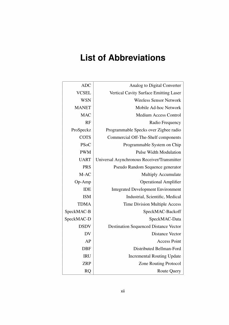
List of Abbreviations
ADC Analog to Digital Converter
VCSEL Vertical Cavity Surface Emitting Laser
WSN Wireless Sensor Network
MANET Mobile Ad-hoc Network
MAC Medium Access Control
RF Radio Frequency
ProSpeckz Programmable Specks over Zigbee radio
COTS Commercial Off-The-Shelf components
PSoC Programmable System on Chip
PWM Pulse Width Modulation
UART Universal Asynchronous Receiver/Transmitter
PRS Pseudo Random Sequence generator
M-AC Multiply Accumulate
Op-Amp Operational Amplifier
IDE Integrated Development Environment
ISM Industrial, Scientific, Medical
TDMA Time Division Multiple Access
SpeckMAC-B SpeckMAC-Backoff
SpeckMAC-D SpeckMAC-Data
DSDV Destination Sequenced Distance Vector
DV Distance Vector
AP Access Point
DBF Distributed Bellman-Ford
IRU Incremental Routing Update
ZRP Zone Routing Protocol
RQ Route Query
xii
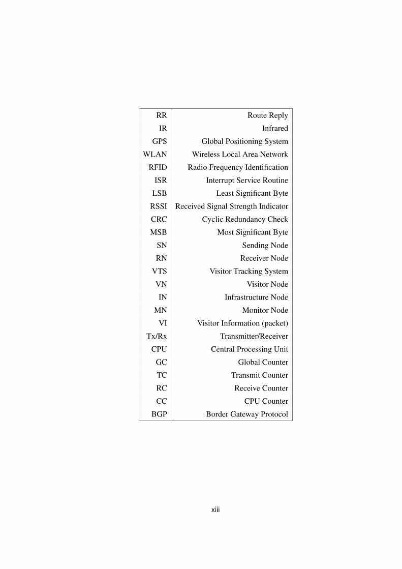
RR Route Reply
IR Infrared
GPS Global Positioning System
WLAN Wireless Local Area Network
RFID Radio Frequency Identification
ISR Interrupt Service Routine
LSB Least Significant Byte
RSSI Received Signal Strength Indicator
CRC Cyclic Redundancy Check
MSB Most Significant Byte
SN Sending Node
RN Receiver Node
VTS Visitor Tracking System
VN Visitor Node
IN Infrastructure Node
MN Monitor Node
VI Visitor Information (packet)
Tx/Rx Transmitter/Receiver
CPU Central Processing Unit
GC Global Counter
TC Transmit Counter
RC Receive Counter
CC CPU Counter
BGP Border Gateway Protocol
xiii
Chapter 1
Introduction
1.1 Rationale
In recent years, there have been significant advances in the technology used to build
Micro-Electro-Mechanical Systems (MEMS), digital electronics, and wireless com-
munications. This has enabled the development of low-cost, low-power, multi-functional
small sensor nodes that can communicate across short distances (2).
There has been a lot of research into routing in wireless sensor networks, as sum-
marised in (1) and (3). Routing in wireless sensor networks is important, as commu-
nication between nodes is central to most applications that use them. According to
Al-Karaki and Kamal (3), routing in wireless sensor networks is different from routing
in IP and Mobile Ad-hoc Networks (MANET) because:
• The large numbers of nodes, that make it expensive to construct a global address-
ing scheme. Furthermore, since several wireless sensor network applications are
data-driven, addressing is not as important.
• Most applications require data to flow from several sensor nodes to a given sink.
• There are tight constraints on energy, processing power, and memory.
• In most application scenarios, most wireless sensor network nodes are stationary,
except for a few mobile nodes, thereby making topological changes infrequent.
Similarly, according to (2), ad-hoc routing techniques are unsuitable for use in
wireless sensor networks because of the larger numbers of nodes, dense deployment,
higher failure rates, frequent topology changes, use of the broadcast (as opposed to the
1

Chapter 1. Introduction 2
point-to-point) communication paradigm, limited power, computational capacities and
memories, and infeasibility of using global identifiers.
Several of the objections raised in (2) and (3) are similar, though a few - regarding
frequency of topological changes and the use of broadcast paradigms - contradict each
other.
MANET nodes are highly mobile, and this mobility produces effects similar to
node failure, i.e., topological changes. There are also wireless sensor applications
where dense deployment and significantly larger numbers of nodes are unnecessary,
and global IDs are necessary. However, the available energy and memory capacity is
highly limited on wireless sensor networks.
Therefore, in this work, we consider whether and how MANET routing algorithms
can be used in wireless sensor networks, and application scenarios of the sort described
in the preceding paragraph are discussed.
1.2 Algorithm Characterisation
The primary question that this work set out to answer is whether MANET routing
algorithms are suitable for use in wireless sensor networks. This could potentially
open up an entirely new class of algorithms for use in wireless sensor networks.
To this end, an exploratory study was carried out, wherein two routing algorithms
used in MANETs were implemented on hardware prototypes of Specknets called the
Prospeckz IIK (4).
The Prospeckz IIK is the second generation of a prototype that was developed in or-
der to “enable the rapid development of Specks” as well as applications for Specks (4).
The Prospeckz IIK uses off-the-shelf components, and includes a radio with adjustable
signal strengths, an 8-bit microcontroller with 32 Kbytes of FLASH and 2 Kbytes of
RAM, and the ability to design analogue circuitries that are software reconfigurable.
The SpeckMAC algorithm developed by K.J. Wong and D.K. Arvind (38), was
used in the MAC layer. This was done because the SpeckMAC algorithm has better
power conservation characteristics than other comparable MAC layer algorithms such
as the B-MAC (27).
The two algorithms implemented were the Destination Sequenced Distance Vector
(DSDV) (26) and the Zone Routing Protocol (ZRP) (15). The first is a proactive -
wherein routes to all nodes are stored within each node - while the latter is a hybrid
routing algorithm - which uses a proactive routing algorithm within defined zones and
Chapter 1. Introduction 3
a reactive algorithm outside these zones (15).
These algorithms were characterised by considering their memory requirements,
power consumption, message delivery latency, and Transmitter/Receiver On-time.
1.3 Applications
In addition to the characterisation of MANET algorithms, we also consider applica-
tions where these routing algorithms could be used in the network layer.
Therefore, in this work, we developed an application running on the Prospeckz IIK,
which used the routing algorithms characterised as enablers.
During the implementation of these applications, we were also able to study the
use of wireless sensor networks in the fields of moving object tracking and ubiquitous
computing.
1.3.1 Visitor Tracking System
The application we envisaged - called the Visitor Tracking System - involved tracking
the approximate location of several mobile nodes in a small building, and feed infor-
mation on location and direction of each node to a single central sink. It was required
that the user at the central sink receive alerts if any mobile node approached restricted
areas within the building.
However, the omni-directional nature of radio waves and multi-path propagation
make accurate location estimation using radios a very difficult and challenging prob-
lem. This is still an open research problem.
Therefore, it was decided that the application would attempt to perform approxi-
mate location estimation on the basis of the signal strength of received radio signals.
The DSDV routing algorithm (26) was used to communicate node location infor-
mation to the sink node. The application’s performance was subsequently charac-
terised by analysing the power consumption, as well as by monitoring the percentage
of time the CPU, Receiver and Transmitter were turned on.
However, the DSDV algorithm is a proactive algorithm, and this, for reasons ex-
plained later on in this document, limits the scale of this application.
Chapter 1. Introduction 4
1.4 Outline
The rest of this thesis is organised as follows:
Chapter 2 delves in considerable depth into the background and context of this
work. It includes a description of Wireless Sensor Networks (WSN)and the hardware
and software platforms used in the development of this work, followed by a brief out-
line of the routing algorithms and applications implemented during the course of this
thesis.
The three chapters that follow describe the implementation of the DSDV algorithm,
the Visitor Tracking System (VTS), and the ZRP algorithm. The discussion considers
the primitives and data structures used therein, and clarifies the operation of these
algorithms using examples.
Chapter 6 contains a discussion of the metrics used to analyse the implementations
described in the previous chapters. The metrics, and the procedures and experimental
setups required to measure them, are presented in great detail in this chapter.
The next three chapters expound on the results obtained upon running the experi-
ments defined in Chapter 6 on the implementations presented in Chapters 3, 4, and 5.
An attempt is made to analyse the significance of the results thus obtained.
The last chapter compares the two algorithms implemented as part of this work,
and attempts to draw conclusions from the comparison. It also explores avenues for
future work.
Chapter 2
Background
In this chapter, a brief discussion is presented of some of the concepts, algorithms,
and hardware platforms that were used during the course of this work. A discussion
of Wireless Sensor Networks (WSN) is followed by a discussion on Specknets, and
the Prospeckz IIK hardware platform that was used to implement the algorithms and
the applications. The next section describes Mobile Ad-hoc Networks (MANETs),
and provides arguments both for and against the use of MANET algorithms in wire-
less sensor networks. Section 2.3 describes the algorithm used in the Medium Access
Control (MAC) layer throughout the thesis - SpeckMac. The fourth section discusses
the MANET routing algorithms which were evaluated on the WSN platform. This is
followed by a discussion of tracking mechanisms used in wireless networks.
2.1 Wireless Sensor Networks
Sensor nodes are low-cost, low-power, multi-functional devices which have a small
form factor and can communicate untethered,using (usually) Radio Frequency (RF)
communication across short distances (2).
Networks of such nodes are called WSNs, and can be deployed in the area of
interest to monitor the physical environment.
They are usually deployed densely in random positions, either inside of, or very
close to the phenomenon that has to be monitored.
Sensor networks can be used in several applications and locations, ranging from a
battlefield to the user’s living room.
In the remainder of this section, we shall present short overviews of the architecture
of sensor nodes and networks, traditional sensor network topology, and the sensor
5
Chapter 2. Background 6
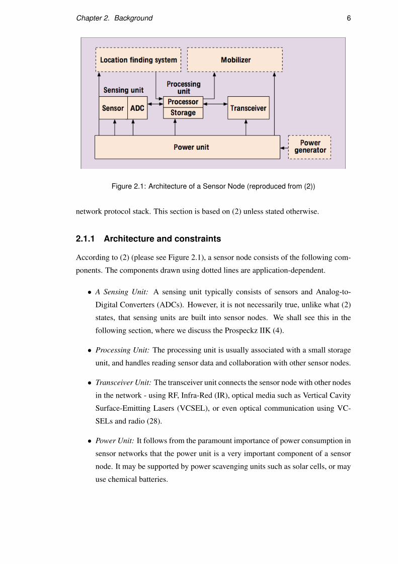
Figure 2.1: Architecture of a Sensor Node (reproduced from (2))
network protocol stack. This section is based on (2) unless stated otherwise.
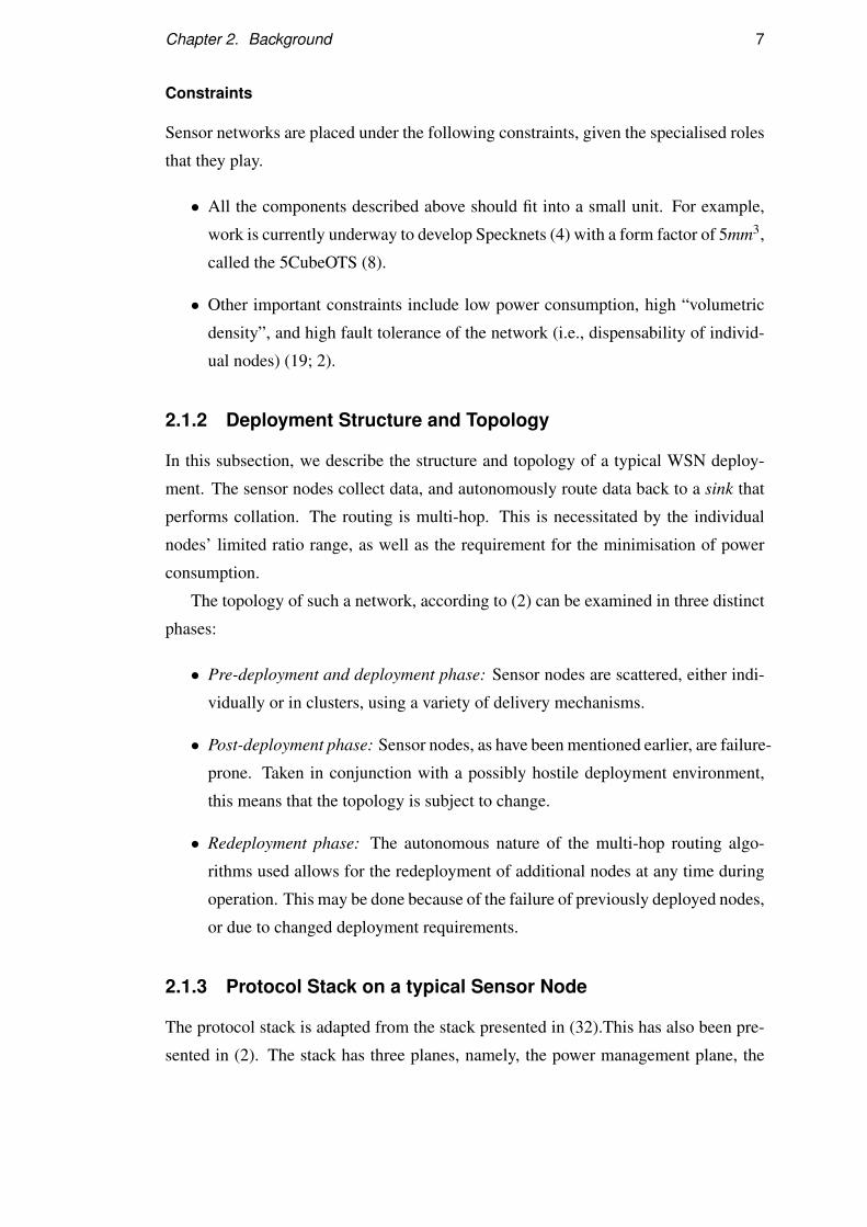
2.1.1 Architecture and constraints
According to (2) (please see Figure 2.1), a sensor node consists of the following com-
ponents. The components drawn using dotted lines are application-dependent.
• A Sensing Unit: A sensing unit typically consists of sensors and Analog-to-
Digital Converters (ADCs). However, it is not necessarily true, unlike what (2)
states, that sensing units are built into sensor nodes. We shall see this in the
following section, where we discuss the Prospeckz IIK (4).
• Processing Unit: The processing unit is usually associated with a small storage
unit, and handles reading sensor data and collaboration with other sensor nodes.
• Transceiver Unit: The transceiver unit connects the sensor node with other nodes
in the network - using RF, Infra-Red (IR), optical media such as Vertical Cavity
Surface-Emitting Lasers (VCSEL), or even optical communication using VC-
SELs and radio (28).
• Power Unit: It follows from the paramount importance of power consumption in
sensor networks that the power unit is a very important component of a sensor
node. It may be supported by power scavenging units such as solar cells, or may
use chemical batteries.
Chapter 2. Background 7
Constraints
Sensor networks are placed under the following constraints, given the specialised roles
that they play.
• All the components described above should fit into a small unit. For example,
work is currently underway to develop Specknets (4) with a form factor of 5mm3,
called the 5CubeOTS (8).
• Other important constraints include low power consumption, high “volumetric
density”, and high fault tolerance of the network (i.e., dispensability of individ-
ual nodes) (19; 2).
2.1.2 Deployment Structure and Topology
In this subsection, we describe the structure and topology of a typical WSN deploy-
ment. The sensor nodes collect data, and autonomously route data back to a sink that
performs collation. The routing is multi-hop. This is necessitated by the individual
nodes’ limited ratio range, as well as the requirement for the minimisation of power
consumption.
The topology of such a network, according to (2) can be examined in three distinct
phases:
• Pre-deployment and deployment phase: Sensor nodes are scattered, either indi-
vidually or in clusters, using a variety of delivery mechanisms.
• Post-deployment phase: Sensor nodes, as have been mentioned earlier, are failure-
prone. Taken in conjunction with a possibly hostile deployment environment,
this means that the topology is subject to change.
• Redeployment phase: The autonomous nature of the multi-hop routing algo-
rithms used allows for the redeployment of additional nodes at any time during
operation. This may be done because of the failure of previously deployed nodes,
or due to changed deployment requirements.
2.1.3 Protocol Stack on a typical Sensor Node
The protocol stack is adapted from the stack presented in (32).This has also been pre-
sented in (2). The stack has three planes, namely, the power management plane, the

Chapter 2. Background 8
mobility management plane, and the task management plane. The stack also consists
of five distinct layers as described below:
• Physical Layer: This layer deals with modulation and Transmission and Recep-
tion techniques.
• Data Link Layer: The focus, in this layer, is on the development of a power-
aware MAC protocol, which minimises collisions, as well as the time for which
the transceiver is turned on.
• Network Layer: This layer primarily deals with routing. However, the presence
or absence of this layer is dependent upon application requirements.
• Transport Layer: This layer maintains data flow, performs congestion control,
and several other tasks which are traditionally performed on transport layers in
wired networks as well. However, in the applications presented in this work, we
do not use the transport layer, and therefore, we shall not discuss this further.
• Application Layer: This layer contains the application software.
This work primarily concerns itself with the implementation of a small subset of
these routing techniques, and therefore, our focus will subsequently be restricted to the
MAC and network layers respectively.
2.2 Specknets and the ProSpeckz IIK
A Speck, as defined in (4), “is designed to integrate sensing, processing and wire-
less networking capabilities in a minute semiconductor grain”. Thousands of Specks,
once deployed, are expected to collaborate as “programmable computational networks
called Specknets”.
As can be seen from these definitions, Specks and Specknets are analogous to the
sensor nodes and WSNs discussed in the previous section. The aim of the Speckled
Computing Project1 is to enable ubiquitous computing, wherein computation will be
performed everywhere, invisible to its users (37).
Communication between nodes on a Specknet are expected to be a combination of
optical and radio communication as discussed in the previous section (28; 4).
1www.specknet.org
Chapter 2. Background 9
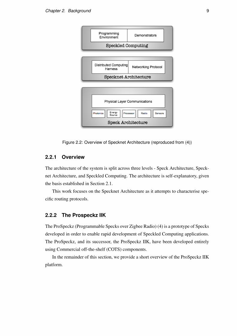
Figure 2.2: Overview of Specknet Architecture (reproduced from (4))
2.2.1 Overview
The architecture of the system is split across three levels - Speck Architecture, Speck-
net Architecture, and Speckled Computing. The architecture is self-explanatory, given
the basis established in Section 2.1.
This work focuses on the Specknet Architecture as it attempts to characterise spe-
cific routing protocols.
2.2.2 The Prospeckz IIK
The ProSpeckz (Programmable Specks over Zigbee Radio) (4) is a prototype of Specks
developed in order to enable rapid development of Speckled Computing applications.
The ProSpeckz, and its successor, the ProSpeckz IIK, have been developed entirely
using Commercial off-the-shelf (COTS) components.
In the remainder of this section, we provide a short overview of the ProSpeckz IIK
platform.

Chapter 2. Background 10
2.2.2.1 Programmable System-on-Chip (PSoC)
The Programmable System-on-Chip (PSoC) (12) family, developed by Cypress Mi-
crosystems, consists of several “Mixed Signal Array with On-Chip Controller” de-
vices. The CY8C29666 chip used on the ProSpeckz IIK belongs to this family.
The PSoC device consists of configurable blocks of analogue and digital logic, and
programmable interconnects.
It also includes an M8C processor (with speeds up to 24MHz), 32 KBytes of Flash
programming storage, and 2 KBytes of SRAM data storage.
The chip consists of four components:
• PSoC Core: This includes the M8C processor, Flash memory (which can emu-
late EEPROM), and the SRAM.
• Digital System: This includes 16 digital PSoC blocks. These blocks support the
incorporation of 8-to-32 bit Timers (13), 8-to-32 bit Pulse Width Modulation
(PWMs) blocks, 8-to-32 bit (down-)Counters (11), an 8-bit Universal Asyn-
chronous Receiver/Transmitter (UART) (14), and Pseudo Random Sequence
(PRS) Generators. There are many more configurations supported, but they are
not relevant to developing an understanding of this work.
• Analog System: This includes 12 configurable blocks, each of which consists
of an Operational Amplifier (Op-Amp) circuit. This allows for the creation of
complex analog signal flows.
• System Resources: System Resources provide “additional capabilities useful for
complete systems” (12), such as digital clock dividers, a Multiply-Accumulate
(M-AC) system, and an integrated switch mode pump (SMP) allowing for the
use of 1.2 V batteries, among others.
PSoC chips can be programmed using an Integrated Development Environment
(IDE) called the PSoC Designer - which was used, for the most part, during the course
of this work. An in-circuit emulator can be used for debugging. Additionally, the
analogue reconfigurability of the PSoC chip allows for quick and easy interfacing of
external sensors to the ProSpeckz IIK.
Chapter 2. Background 11
2.2.2.2 The CC2420 Radio
The ProSpeckz IIK uses the CC2420 transceiver in order to implement radio commu-
nications. The CC2420 is a single-chip, IEEE 802.15.4 compliant RF transceiver, and
communicates using the 2.4 GHz (2,400−2,583 MHz) Industrial, Scientific, Medical
(ISM) band.
It is low-power, runs at a low voltage (18.8mA at 3.3V on the Prospeckz IIK), and
provides an effective data rate of 250 Kbps.
The CC2420 can transmit at several different signal strengths, ranging from 0 dBm2
(Rx: 18.8 mA, Tx: 17.4 mA) to -25 dBm (Tx: 8.5 mA). This can be set using integer
arguments ranging from 0 to 31, with the latter corresponding to transmission (Tx)
power of 17.4 mA.
Since it provides extensive hardware support for packet handling, data buf fer-
ing, encryption and authentication, burst transmissions, clear channel assessment, link
quality, and packet timing information, it reduces the load on the host controller.
Additionally, the ProSpeckz IIK uses 2.4 GHz matched antenna and filter cir-
cuitries to improve power transfer from circuitry to the transmission medium (air).
2.3 The MAC Layer in Wireless Sensor Networks
A MAC protocol on sensor networks has the following requirements:
• Creation of a network infrastructure.
• Fair and efficient sharing of communication resources.
• Most importantly, the minimisation of the power consumed.
The closest peers to sensor networks, according to (2) are Bluetooth and MANETs.
However, Bluetooth communication is essentially of a Master-Slave nature, allowing
for the use of time-division multiple access (TDMA) scheduling. And in the case of
MANETs, power consumption minimisation is not as important as it is on WSNs.
This is because the batteries on the devices used therein are usually larger, and can be
replaced by the user.
MAC protocols can be classified on the basis of the the degree of centralisation
(38). MAC protocols can thus be classified either as centralised or decentralised.2dBm is a power ratio in decibels (dB) of the measured power, referenced to one milliwatt, and used
to measure absolute power in radio, microwave, and fibre optic transceivers.
Chapter 2. Background 12
In the former category, a base station or cluster head ensures collision-free opera-
tion within the network or cluster. Algorithms using TDMA fall within this category.
As mentioned earlier in this section, this approach is used in Bluetooth (for instance),
and cannot be applied to wireless sensor networks where all the nodes are equally
energy-constrained.
Decentralised MAC protocols deal with the aforementioned deficiencies, and can
be classified as being either “scheduled” or “random-access”. Examples of the former
include S-MAC (39) and T-MAC (35). These protocols use time slots which are much
larger than those used in TDMA based centralised schemes, in order to obviate the need
for tight time synchronisation. Random-access MAC protocols allow nodes to access
the shared medium “on-demand”, and do not require scheduling or synchronisation
(unlike the other classes of algorithms described above). Examples of this approach
include the B-MAC (27) and SpeckMAC (38) algorithms.
This work uses the SpeckMAC algorithm in the MAC layer of the routing protocols
adapted as part of this work. Therefore, the next section provides the reader with a short
description of SpeckMAC, and the rationale behind the choice of SpeckMAC.
2.4 SpeckMAC
SpeckMAC (38) is a “low power, distributed, unsynchronised, random-access” MAC
protocol that provides support for low data rate communication on wireless sensor
networks.
Random access MAC protocols allow nodes to access the channel without requiring
synchronisation or scheculing. SpeckMAC uses in-channel signalling to wake desti-
nation nodes up3.
SpeckMAC transfers the communication costs to the transmission of data, i.e., the
receiver is turned on for as short a period as possible at the expense of a longer transmit-
ted packet. This choice is informed by the low data-rates (low numbers of transmitted
packets) and high nodal density (number of receptions > number of transmissions) on
WSNs.
As a result of this, radio receivers are kept turned off, and are turned on only at
specific intervals of time, Tinterval .
3This is because radio receivers are automatically switched off in order to minimise power consump-tion.
Chapter 2. Background 13
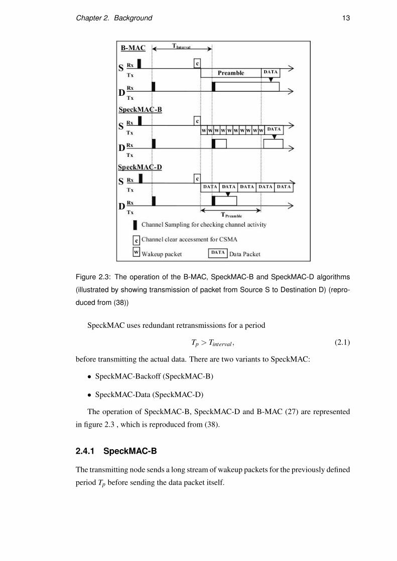
Figure 2.3: The operation of the B-MAC, SpeckMAC-B and SpeckMAC-D algorithms
(illustrated by showing transmission of packet from Source S to Destination D) (repro-
duced from (38))
SpeckMAC uses redundant retransmissions for a period
Tp > Tinterval, (2.1)
before transmitting the actual data. There are two variants to SpeckMAC:
• SpeckMAC-Backoff (SpeckMAC-B)
• SpeckMAC-Data (SpeckMAC-D)
The operation of SpeckMAC-B, SpeckMAC-D and B-MAC (27) are represented
in figure 2.3 , which is reproduced from (38).
2.4.1 SpeckMAC-B
The transmitting node sends a long stream of wakeup packets for the previously defined
period Tp before sending the data packet itself.
Chapter 2. Background 14
When a node switches its receiver on and notices that the medium is busy, it listens
in. If it receives a data packet, it goes back to idle mode after completing reception.
On the other hand, if it receives a wakeup packet, it then switches the receiver off, and
turns it back on when the stream of wakeup packets gives way to the data packet. The
node then returns to sampling the channel periodically as described above.
2.4.2 SpeckMAC-D
In this case, the transmitting node performs redundant retransmissions of the data
packet itself, thereby sending a stream of data packets for a period defined by Tp +Td ,
where Td is the time required to transmit a single data packet, and Tp is an integral
multiple of Td . A data packet is padded with a 3 byte long preamble.
When a node samples the channel, and finds the medium busy, it listens in to com-
plete reception of a data packet, and then turns the receiver off for a period of Tinterval .
Subsequently, it continues to listen periodically for packets.
2.4.3 Why SpeckMAC?
There are two reasons why SpeckMAC was used in the MAC layer for the evaluation
of the routing algorithms implemented as part of this work. These are summarised
below:
• SpeckMAC is a decentralised, random-access MAC protocol. The advantages
of this class of algorithms is described in Section 2.3.
• B-MAC was the only other algorithm in the same class that was under consid-
eration, and SpeckMAC performs considerably better than B-MAC with respect
to power consumption - and by extension, battery life. Experiments performed
in (38) indicate that SpeckMAC-B and SpeckMAC-D improve battery life by up
to 83.5% and 117.9% respectively, when compared to B-MAC.
Additionally, since the performance improvements upon using SpeckMAC-D were
shown in (38) to be considerably higher, it was chosen as the MAC protocol over
SpeckMAC-B.
Chapter 2. Background 15
2.5 Routing in Wireless Sensor Networks
As discussed in Section 2.1, WSNs require multi-hop routing algorithms due to limited
radio ranges of the individual nodes. According to (3; 2; 1), routing algorithms in
WSNs must be designed keeping the following requirements and constraints in mind:
• Power efficiency is the most important consideration due to the limited capacity
of a sensor node.
• The WSN has to be self-organising.
• WSNs are mostly data-centric.
• Position awareness is extremely important in many WSN applications.
• Data collected by sensor nodes may contain large amounts of redundancy. There-
fore, in-network aggregation would have to be performed.
Additionally, it is stated in (3) that:
• The large numbers of sensor nodes in typical WSN deployments make it impos-
sible to build a global addressing scheme.
• Post-deployment, WSN nodes are stationary in most cases. In some applications,
however, sensor networks may be allowed to move and change their location
(although with low mobility)
Furthermore, it is stated in (2) that:
• Sensor nodes mainly use a broadcast communication paradigm, whereas most ad
hoc network routing algorithms use the point-to-point communication paradigm.
On the basis of some of the arguments put forth in the two preceding lists, the
authors of (2) state that protocols and algorithms proposed for traditional wireless ad
hoc networks are “not well-suited to the unique features and application requirements
of sensor networks”.
In this work, part of our focus is to validate the veracity of this assertion by
implementing and evaluating two algorithms designed for and traditionally used in
MANETs.
Chapter 2. Background 16
2.5.1 Classification of routing protocols
Routing protocols are classified in (15) to be of three types:
• Proactive routing algorithms: In proactive routing algorithms, each node stores
information on routes to every other node in the network. The settling time for
a network using an algorithm of this sort is extremely high, and the number of
messages exchanged in order to maintain route information can grow large very
quickly, limiting the scalability of such algorithms.
• Reactive routing algorithms: Reactive routing algorithms require each node to
store routes only to its immediate neighbours, and determine multi-hop routes
as required. This reduces the routing table maintenance overhead, but increases
the time required to send a message as the path has to be determined each time a
packet has to be transmitted across multiple hops.
• Hybrid routing algorithms: Hybrid routing algorithms combine the strengths
of both reactive and proactive algorithms, and use a proactive scheme within
a given radius, and a reactive scheme to determine routes to nodes outside the
radius. The radius may be determined by several metrics, including number of
hops.
2.5.2 Classification of WSN routing protocols
The classification of WSN routing algorithms, according to (3), can be performed on
the following bases:
• According to network structure:
– Flat: In a flat network, all the nodes play the same role.
– Hierarchical: The network is clustered, so that cluster heads do the work.
Different nodes can be cluster-heads at different times.
– Location-Based: Positioning information is used in networks of this nature
to relay data to a specific portion/region of the network.
– Multipath-based
– Query-based
– Quality of Service (QoS)- based
Chapter 2. Background 17
– Coherent-based
However, as described above, we are not concerned with routing protocols tra-
ditionally used in WSNs. Therefore, in the following sections, we discuss the two
MANET routing algorithms that were implemented during the course of this thesis.
2.6 Destination-Sequenced Distance-Vector Routing (DSDV)
The first MANET algorithm that we implemented as part of this work is called the
Destination-Sequenced Distance Vector (DSDV) routing algorithm (26). According to
the classification scheme presented in (15), it is a proactive routing algorithm.
The DSDV algorithm is a Distance Vector (DV) based routing algorithm designed
for use in MANETs, which are defined by Perkins et al. (26) as the “cooperative
engagement of a collection of Mobile Hosts without the required intervention of any
centralised Access Point (AP)”.
It operates each node as a “specialised router” (26) which periodically advertises its
knowledge of the network with the other nodes in the network. It makes modifications
to the basic Bellman-Ford routing algorithms (9), thereby doing away with the count-
to-infinity problem.
The algorithm is designed for portable computing devices such as laptops who have
energy and processing capabilities far beyond that of a typical WSN node. However,
it is our contention that this algorithm can be used on WSNs, and this work attempts
to modify the algorithm to have it run on WSNs (albeit of constrained size).
In the rest of this section, we present a short overview of DV based algorithms,
followed by a discussion of the operation of, and issues with, the DSDV algorithm. It
is based on (26) unless explicitly mentioned otherwise.
2.6.1 Distance Vector routing
Every node i in the network maintains distances to every other node in the network.
This distance is chosen from the shortest distance dix = min(di j + d jx), where x is the
destination node, and j is a neighbour of i. Each node keeps track of the distances
between itself and every other node in the network, and periodically broadcasts its
current estimate of the shortest distance to every other node in the network to all of its
neighbours. This algorithm is known as the Distributed Bellman-Ford (DBF) algorithm
(21).
Chapter 2. Background 18
However, DV algorithms such as the DBF algorithm suffer from the count-to-
infinity problem (21). This can be solved using the split-horizon and poisoned-reverse
mechanisms. However, these solutions are not entirely compatible with the essentially
broadcast nature of radio communications.
The DSDV algorithm works similar to other DV algorithms in that it broadcasts
routing table entries to each of its neighbours, where the routing table entries contain
entries for every node in the network.
2.6.2 Sequence Numbers
Each routing table entry contains the destination address, the number of hops to reach
the destination, the next hop along the path to the destination, and the sequence num-
ber of the latest information received regarding the destination. Routing table entries
with newer (read: higher) sequence numbers supercede entries with older sequence
numbers. When faced with a choice between two routing table entries with the same
sequence number, the entry with the lower value of the metric (in our implementation,
the number of hops) is chosen.
Every destination stamps sequence numbers with consecutive even numbers. Every
receiver in turn broadcasts this information to its neighborus, incrementing the value
of the metric.
2.6.3 Broken Links
A broken link is described by a metric of ∞. Whenever a link between a destination
and a neighbour breaks, the neighbour changes the link distance stored to to ∞ and
increments the sequence number by 1, i.e., the next highest odd number. If any node
receiving information of a link break (with a distance metric of ∞) has a routing table
entry with a later (even) sequence number, it broadcasts this information to all of its
neighbours.
2.6.4 Full Routing Table Dump vs Incremental Routing Update
The DSDV algorithm defines two kinds of routing table updates. The first is called an
Incremental Routing Update (IRU), where only those routing table entries that have
changed since the last IRU was sent are transmitted. The second, called the Full Rout-
ing Table Dump (FRTD), transmits every routing table entry in the node’s routing table.
Chapter 2. Background 19
The latter is done less frequently, and then only when there is not much node move-
ment (i.e., no IRUs have been sent in awhile). An IRU should ideally fit inside a single
network layer packet, whereas a FRTD will most likely require multiple such packets,
even in small networks.
Perkins and Bhagwat (26) also underline the need for a mechanism by which it is
determined if a change in a routing table entry is significant enough for it to be included
in an IRU message.
2.6.5 Preventing Routing Table Fluctuation
In order to prevent a continuous stream of routing updates froma given node, it is
suggested in (26) that two different routing tables be used - one each for advertisement
and forwarding respectively; with the former being updated less frequently than the
latter.
2.6.6 Issues with the DSDV Algorithm
We identified the following problems with implementing the DSDV algorithm in WSNs
such as Specknets - primarily due to the tighter memory and power constraints faced
in WSNs.
• Transmission of FRTDs when there is no change in the network would waste
transmitter power, and can be done away with.
• Maintaining two distinct routing tables would be a waste of memory. A simpler
approach would be to delay transmission of routing updates, in order to allow
for the best routes to be available before IRUs are transmitted. Also, in order to
prevent fluctuations caused by nodes that spasmodically appear to be neighbours,
an anti-flap mechanism may be used4
2.7 Zone Routing Protocol
The Zone Routing Protocol (ZRP) algorithm was first proposed for use in ad-hoc net-
works in (15). It is a hybrid routing algorithm, which uses a proactive routing algo-
4The DSDV implementation used within the ZRP implementation solved this problem by using IRUsto discover neighbours. This also reduced the total number of transmissions, as well as the probabilityof a stray transmission being received.
Chapter 2. Background 20
Figure 2.4: A network divided into zones with a zone radius of 2
rithm within a given zone (with a user-defined radius), and a reactive scheme outside
the zone. The rest of this section describes the ZRP algorithm in greater detail.
2.7.1 Basic Operation
The network is divided into a series of overlapping zones. The radius of the zones may
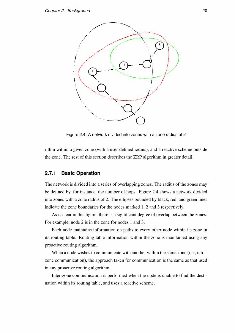
be defined by, for instance, the number of hops. Figure 2.4 shows a network divided
into zones with a zone radius of 2. The ellipses bounded by black, red, and green lines
indicate the zone boundaries for the nodes marked 1, 2 and 3 respectively.
As is clear in this figure, there is a significant degree of overlap between the zones.
For example, node 2 is in the zone for nodes 1 and 3.
Each node maintains information on paths to every other node within its zone in
its routing table. Routing table information within the zone is maintained using any
proactive routing algorithm.
When a node wishes to communicate with another within the same zone (i.e., intra-
zone communication), the approach taken for communication is the same as that used
in any proactive routing algorithm.
Inter-zone communication is performed when the node is unable to find the desti-
nation within its routing table, and uses a reactive scheme.
Chapter 2. Background 21
Both inter- and intra-zone communication are described in greater detail in the
forthcoming sections.
2.7.2 Intra-zone communication in ZRP
A proactive routing scheme is used for intra-zone communication using the ZRP algo-
rithm, as mentioned in the previous section. The proactive routing algorithm used can
vary5.
Communication involves the following steps:
1. The source node tries to determine whether an entry for the destination node
exists in its routing table.
2. It then forwards the packet to the destination node by sending the packet to the
next hop along the path to the destination node (if the route has multiple hops).
If no entry is found for the destination node in the routing table of the source node,
then either the destination doesn’t exist (or has failed), or the destination node is not
within the zone of the source node. In the latter case, the inter-zone communication
techniques described in the following section are used.
2.7.3 Inter-zone communication
A reactive scheme is used for inter-zone communication using the ZRP algorithm.
Inter-zone communication is used by a source node under the circumstances outlined
in the previous section. The steps involved may be described as followed:
1. If the source node finds that the destination node is not within its zone, it sends a
Route Query (RQ) packet to each of the nodes at the boundary of its zone, called
the zone ending nodes, using the intra-zone routing algorithm. It then waits for
responses for a pre-determined period of time.
2. Each of the zone ending nodes examines the final destination specified in the
route query message.
If a route to the destination is stored in the routing table of the zone ending
node, the node sends a Route Reply (RR) packet back to the source node along
the path the query message arrived along.5The DSDV algorithm was used for intra-zone communication in the implementation developed as
part of this work.
Chapter 2. Background 22
If not, the node forwards the query messages along to each of the nodes at
the end of its zone (excluding nodes that have already received the message).
3. The approach used is, thus, a form of controlled, directional flooding.
4. Upon receipt of the route reply message, the source node stores the path and
sends a data message along it6. If no route reply messages are received before
timer expiry at the source node, it reports failure.
2.7.4 Properties of the ZRP routing algorithm
Some of the properties of the ZRP routing algorithm include:
• ZRP has good scalability; by suitably adjusting the zone radius, it is possible
to allow for communication in much larger networks than is possible using a
proactive routing mechanism such as DSDV.
• ZRP performs better than reactive schemes, especially if a large proportion of
communication takes place across short distances. This is because the time re-
quired for route determination for intra-zone communication in ZRP is much
lower than in reactive algorithms, which in turn is due to the use of a proactive
scheme for intra-zone communication.
2.8 Tracking in WSNs
As part of this work, we considered the utility of MANET algorithms for use in WSN
applications. The application under consideration was a tracking application, where
sensor nodes were used to determine the (relative) location of mobile users in a built-
in environment. In this section, therefore, we review some of the approaches taken to
perform tracking in WSNs. The section concludes with a brief overview of the simple
mechanism used in the application implemented herein.
The major approaches towards tracking include the use of in-building Infrared (IR)
networks (36; 5), using wide-area cellular networks (33; 22; 18), and the Global Posi-
tioning System (GPS) (24).
However, all of these approaches are inherently inapplicable to the application do-
main under consideration due to different reasons.
IR networks are inapplicable because:6An implementation improvement could be the caching of discovered inter-zone routes.
Chapter 2. Background 23
• Their performance is adversely affected by sunlight.
• IR transceivers cannot be used for data transmission.
• IR networks work out to be too expensive.
Conversely, approaches used for location tracking in cellular networks are inappli-
cable indoors. GPS systems are too expensive, and are inefficient inside buildings (as
buildings block GPS transmissions).
A fourth approach, most applicable to the application domain under consideration,
is to use RF signals for location estimation and tracking in built environments. To the
best of our knowledge, all the published work in this area has taken Wireless Local
Area Networks (WLAN) which use the IEEE 802.11 standard (10).
(6) discusses an approach called RADAR where WLANs are used to achieve ac-
curate user location and tracking. This uses signal strength information obtained from
multiple receivers to allow for the triangulation of the user’s coordinates.
Bahl et al (7) make significant improvements to the existing RADAR system (6) in
order to minimise problems caused by environmental changes (such as changes in the
number of people, obstructions, and temperature). It also extends the RADAR system
to take multi-floor environments into consideration.
Another location system worth mentioning is LANDMARC, developed by Ni et al
in (25), wherein Radio Frequency Identification (RFID) technology is used for locating
objects indoors.
Smailagic and Kogan (30) also describe a triangulation-based approach using an
IEEE 802.11b (10) wireless network. The approach described therein is client-centric;
that is, the client obtains signal strengths from multiple APs, which in turn is used
for position calculation. This is a triangulation-based remapped interpolated approach,
and is termed CMU-TMI.
The location sensing mechanism used in the application implemented as part of this
work is simpler and more coarse-grained than those used in RADAR or CMU-TMI, as
it performs location estimation on the basis of the minimum received signal strength.
This mechanism is described in greater detail in Chapter 4.
2.9 Summary
This chapter presented the reader with a basic introduction to the areas covered in this
thesis. Starting with a sketch of the architecure, constraints, and deployment structures
Chapter 2. Background 24
of WSNs, the reader was introduced to Specknets and the hardware platform used for
this work, the ProSpeckz IIK. This was followed by a discussion of the MAC layer in
WSNs and the SpeckMAC MAc algorithm used in the MAC layer of all the algorithms
and applications developed as part of this thesis. The discussion subsequently shifted
to routing in WSNs, with special emphasis on the MANET algorithms implemented
herein; namely, the DSDV and ZRP routing algorithms. The last section presented the
reader with a survey of tracking mechanisms, and their applicability to WSNs.
The three chapters that follow delve into the algorithms and applications imple-
mented in considerable depth.
Chapter 3
Implementation of the DSDV Algorithm
In this chapter, we describe the implementation of the DSDV algorithm on the Prospeckz
IIK (4). In the first section, the protocol stack used for the DSDV algorithm is de-
scribed. This is followed in the next section with a description of the data structures
used in the DSDV algorithm - namely the packet formats and the routing table struc-
ture. After considering an operational example of the DSDV algorithm, this chapter
concludes with a short summary of the topics presented.
3.1 Protocol Stack
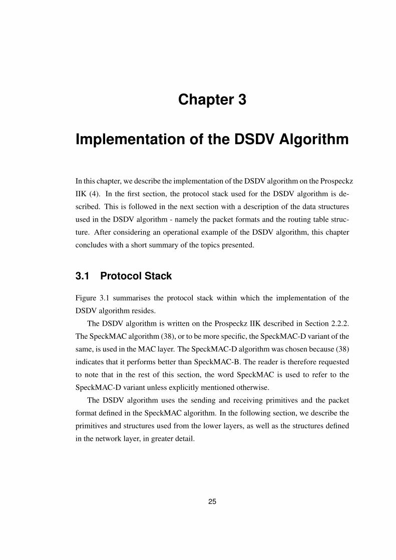
Figure 3.1 summarises the protocol stack within which the implementation of the
DSDV algorithm resides.
The DSDV algorithm is written on the Prospeckz IIK described in Section 2.2.2.
The SpeckMAC algorithm (38), or to be more specific, the SpeckMAC-D variant of the
same, is used in the MAC layer. The SpeckMAC-D algorithm was chosen because (38)
indicates that it performs better than SpeckMAC-B. The reader is therefore requested
to note that in the rest of this section, the word SpeckMAC is used to refer to the
SpeckMAC-D variant unless explicitly mentioned otherwise.
The DSDV algorithm uses the sending and receiving primitives and the packet
format defined in the SpeckMAC algorithm. In the following section, we describe the
primitives and structures used from the lower layers, as well as the structures defined
in the network layer, in greater detail.
25
Chapter 3. Implementation of the DSDV Algorithm 26
Figure 3.1: DSDV protocol stack
3.2 Primitives and Data Structures
In this section, the sending and receiving primitives (defined in the MAC layer) used
in the network layer are described. This is followed by a description of the MAC
layer packet structure used, the mechanisms used for packing the network layer data
structures into the MAC layer packet format, and the packet structures defined in the
network layer.
3.2.1 MAC Layer Primitives
The SpeckMAC algorithm described in Section 2.4 provides several primitives to allow
for the transmission and reception of data from other nodes over the CC2420 radio.
The primitives used in the implementation of the DSDV algorithm are described in
this section.
3.2.1.1 SpeckMAC Blocking Send Primitive
The blocking send primitive does not return until the packet passed to it as an argu-
ment has been successfully sent. Since this reduces the complexity of the code in the
network layer, this primitive was extensively used in the implementation of the DSDV
algorithm.
The implementation characterised herein does not use a scheduler to schedule the
transmission of multiple packets from the network layer. It is, however, worthwhile,
Chapter 3. Implementation of the DSDV Algorithm 27
Figure 3.2: Basic Packet Structure (with DSDV-specific extensions)
noting that the implementation of the ZRP algorithm (described in Chapter 5) uses a
scheduler.
3.2.1.2 Receiving Packets using SpeckMAC
The SpeckMAC algorithm periodically switches the node radio on. When the radio
senses activity in the medium1, it listens in until it has received a whole data packet.
Upon completion of reception, an interrupt which handles the received packet and
checks for errors is triggered.
The packet handler for the DSDV algorithm is called from within the SpeckMAC
Interrupt Service Routine (ISR).
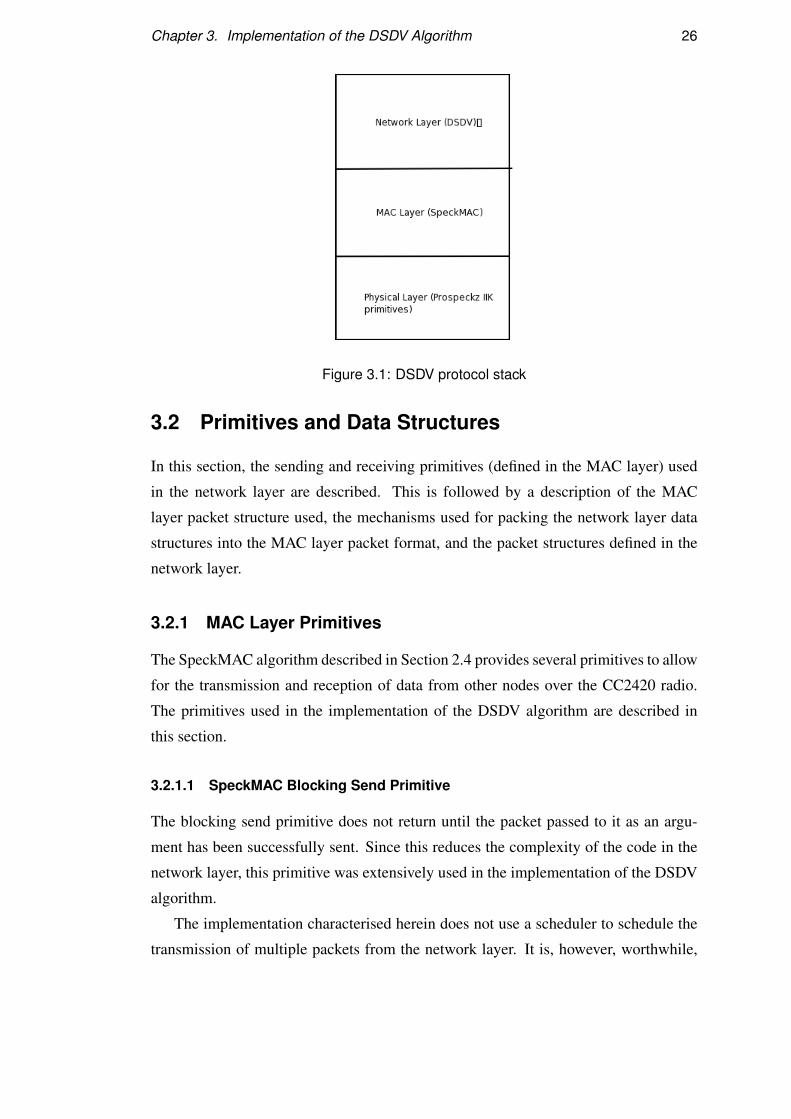
3.2.1.3 Packet Format
The packet format used in the MAC layer of the implementation is summarised in
Figure 3.2.
To maintain separation between the layers, it would have been necessary to encap-
sulate the entire network layer packet inside the data field of the MAC layer packet.
However, the design decision was taken to sacrifice modularity in favour of perfor-
mance. Hence, the packet header was modified to include DSDV-specific headers.
This is because the size of the data field is limited. Therefore, using the data field to
store DSDV-specific information would be a waste of valuable space, and would also
1This is indicative of packet transmission by another node in the network.
Chapter 3. Implementation of the DSDV Algorithm 28
result in an increase in the transmission time for the packet2.
The fields in Figure 3.2 that are marked in red are DSDV-specific fields, whereas
those marked in black are the MAC layer-specific fields. The purpose of the fields in
the structure are as described below:
• MAC Layer-specific fields:
Cyclic Redundancy Check (CRC): CRC is an error detection method which
typically involves the calculation of a two-byte checksum of a data block, and
is used to detect the accidental alteration of data during transmission or storage.
The Least Significant Byte (LSB) of the CRC is loaded into this 1 byte field.
Received Signal Strength Indicator (RSSI): RSSI is a measure of the strength
(and not necessarily the quality) of the received signal strength in a wireless
network (31). The Most Significant Byte (MSB) of the two-byte CRC is loaded
into this 1 byte field by the MAC layer whenever a packet is transmitted.
Destination Address: This field holds the ID of the node that is the packet’s
final destination.This field is 16 bits long, and thus, the implementation of the
DSDV theoretically allows for 65,536 distinct nodes in the network. However,
in practice, only 13 of these bits are used, thereby restricting the number of nodes
to 8191.
Source Address: This field, which is also 16 bits long, holds the address of
the source of the packet, i.e., the node that constructed the original packet.
• Network Layer-specific fields:
DSDV Address: This 2 byte field holds the address of the next node along
the path from the source to the destination that the packet is to be forwarded to.
Sequence Number: This field is also 2 bytes long, and is used to hold the
sequence number of the DSDV algorithm packet transmitted from that source.
The reasons behind the utilisation of sequence numbers are discussed in Section
2.6.
• Data length: This field is 8 bits long, and indicates the size of the payload in
bytes, to a maximum of 32.
2It must be noted here that the MAC layer implementation transmits the entire header with eachpacket.
Chapter 3. Implementation of the DSDV Algorithm 29
Figure 3.3: Packet Types used in the DSDV algorithm
• Payload: The payload field is a character array of length 32. Consequently, the
maximum payload size is limited to 256 bits. The number of bytes used in the
payload are indicated, as described above, in the data length field.
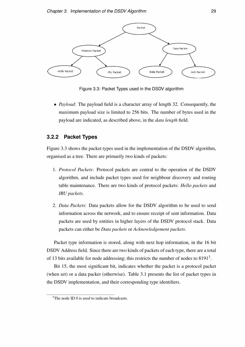
3.2.2 Packet Types
Figure 3.3 shows the packet types used in the implementation of the DSDV algorithm,
organised as a tree. There are primarily two kinds of packets:
1. Protocol Packets: Protocol packets are central to the operation of the DSDV
algorithm, and include packet types used for neighbour discovery and routing
table maintenance. There are two kinds of protocol packets: Hello packets and
IRU packets.
2. Data Packets: Data packets allow for the DSDV algorithm to be used to send
information across the network, and to ensure receipt of sent information. Data
packets are used by entities in higher layers of the DSDV protocol stack. Data
packets can either be Data packets or Acknowledgement packets.
Packet type information is stored, along with next hop information, in the 16 bit
DSDV Address field. Since there are two kinds of packets of each type, there are a total
of 13 bits available for node addressing; this restricts the number of nodes to 81913.
Bit 15, the most significant bit, indicates whether the packet is a protocol packet
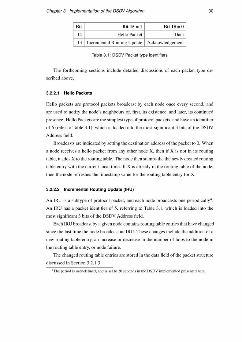
(when set) or a data packet (otherwise). Table 3.1 presents the list of packet types in
the DSDV implementation, and their corresponding type identifiers.
3The node ID 0 is used to indicate broadcasts.
Chapter 3. Implementation of the DSDV Algorithm 30
Bit Bit 15 = 1 Bit 15 = 0
14 Hello Packet Data
13 Incremental Routing Update Acknowledgement
Table 3.1: DSDV Packet type identifiers
The forthcoming sections include detailed discussions of each packet type de-
scribed above.
3.2.2.1 Hello Packets
Hello packets are protocol packets broadcast by each node once every second, and
are used to notify the node’s neighbours of, first, its existence, and later, its continued
presence. Hello Packets are the simplest type of protocol packets, and have an identifier
of 6 (refer to Table 3.1), which is loaded into the most significant 3 bits of the DSDV
Address field.
Broadcasts are indicated by setting the destination address of the packet to 0. When
a node receives a hello packet from any other node X, then if X is not in its routing
table, it adds X to the routing table. The node then stamps the the newly created routing
table entry with the current local time. If X is already in the routing table of the node,
then the node refreshes the timestamp value for the routing table entry for X.
3.2.2.2 Incremental Routing Update (IRU)
An IRU is a subtype of protocol packet, and each node broadcasts one periodically4.
An IRU has a packet identifier of 5, referring to Table 3.1, which is loaded into the
most significant 3 bits of the DSDV Address field.
Each IRU broadcast by a given node contains routing table entries that have changed
since the last time the node broadcast an IRU. These changes include the addition of a
new routing table entry, an increase or decrease in the number of hops to the node in
the routing table entry, or node failure.
The changed routing table entries are stored in the data field of the packet structure
discussed in Section 3.2.1.3.4The period is user-defined, and is set to 20 seconds in the DSDV implemented presented here.
Chapter 3. Implementation of the DSDV Algorithm 31
3.2.2.3 Data Packet
A data packet is used to send data to any other node in the routing table of the Sending
Node (SN). A data packet is constructed as follows:
• The Source address is set to the node’s ID.
• The Destination address is set to the address of the packet’s destination.
• The DSDV address is set to the XOR of the packet type identifier (refer to Table
3.1) and the address of the next hop to the destination specified in the Destination
address field. If the destination node is 1 hop away, then the DSDV address is
set to the same value as the destination address.
• The Sequence number field is loaded with the sequence number of the data
packet being sent.
• The data to be sent is loaded into the packet’s Payload.
• The Data length field is loaded with the number of bytes of the payload used.
3.2.2.4 Acknowledgement Packet
Acknowledgement packets are used to certify receipt of a Data packet, and is sent
by the Receiving Node (RN) to the Sending Node (SN). Acknowledgement packets
typically contain no data, and are constructed just as data packets are - except for the
Sequence number field, which stores the sequence number of the data packet being
acknowledged.
Acknowledgement packets can be used to implement delivery guarantees.
3.2.3 The Routing Table
The routing table contains information about every other node in the network. This
information includes the address of the RN, the number of hops to it, and the next hop
through which any packets to the RN must be routed.
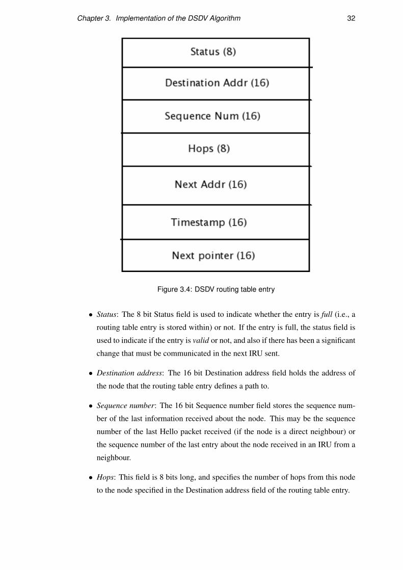
The routing table in the DSDV implementation is structured as a circular list. Fig-
ure 3.4 shows the structure of a single entry in the routing table, and Figure 3.5 shows
the organisation of the links between the nodes in the routing table.
The fields in a routing table entry include:
Chapter 3. Implementation of the DSDV Algorithm 32
Figure 3.4: DSDV routing table entry
• Status: The 8 bit Status field is used to indicate whether the entry is full (i.e., a
routing table entry is stored within) or not. If the entry is full, the status field is
used to indicate if the entry is valid or not, and also if there has been a significant
change that must be communicated in the next IRU sent.
• Destination address: The 16 bit Destination address field holds the address of
the node that the routing table entry defines a path to.
• Sequence number: The 16 bit Sequence number field stores the sequence num-
ber of the last information received about the node. This may be the sequence
number of the last Hello packet received (if the node is a direct neighbour) or
the sequence number of the last entry about the node received in an IRU from a
neighbour.
• Hops: This field is 8 bits long, and specifies the number of hops from this node
to the node specified in the Destination address field of the routing table entry.
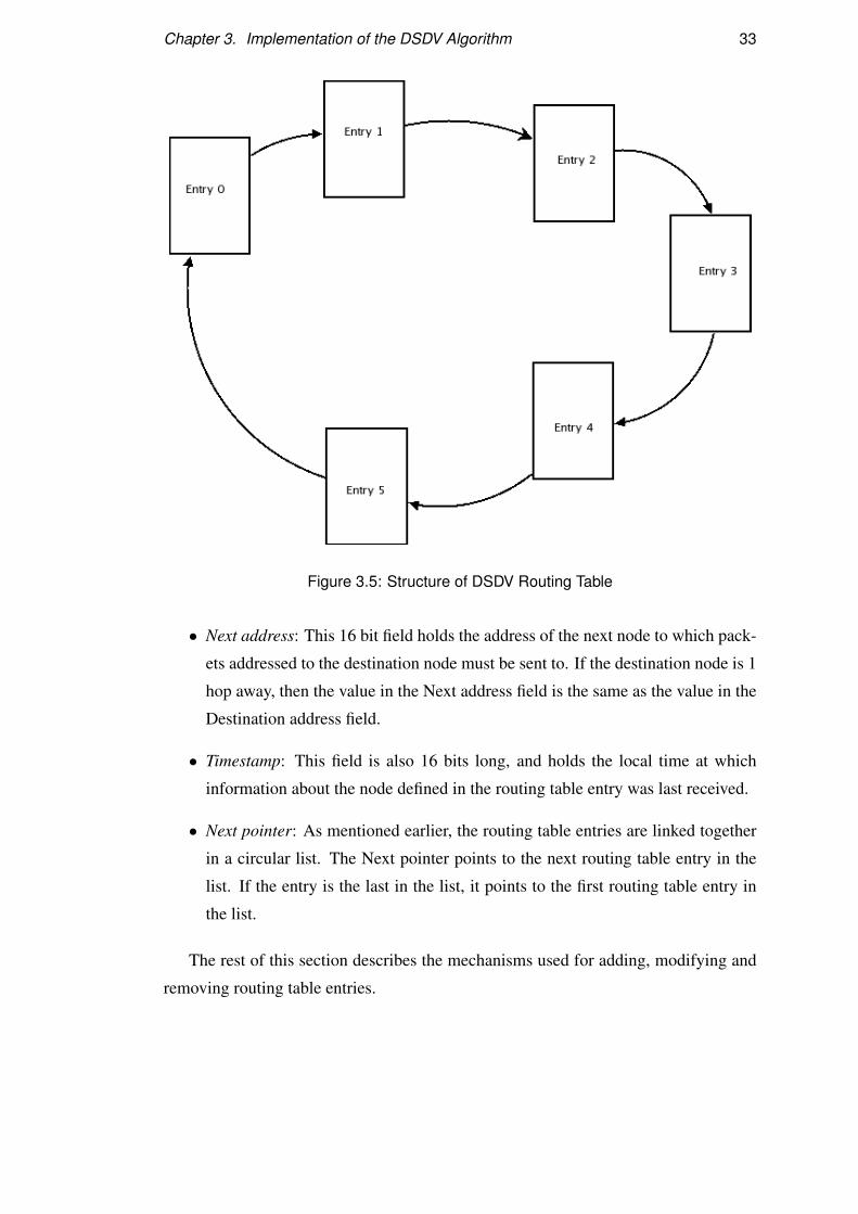
Chapter 3. Implementation of the DSDV Algorithm 33
Figure 3.5: Structure of DSDV Routing Table
• Next address: This 16 bit field holds the address of the next node to which pack-
ets addressed to the destination node must be sent to. If the destination node is 1
hop away, then the value in the Next address field is the same as the value in the
Destination address field.
• Timestamp: This field is also 16 bits long, and holds the local time at which
information about the node defined in the routing table entry was last received.
• Next pointer: As mentioned earlier, the routing table entries are linked together
in a circular list. The Next pointer points to the next routing table entry in the
list. If the entry is the last in the list, it points to the first routing table entry in
the list.
The rest of this section describes the mechanisms used for adding, modifying and
removing routing table entries.
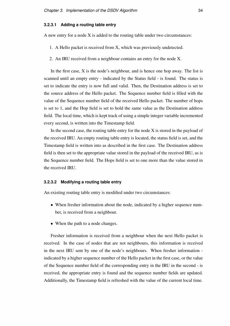
Chapter 3. Implementation of the DSDV Algorithm 34
3.2.3.1 Adding a routing table entry
A new entry for a node X is added to the routing table under two circumstances:
1. A Hello packet is received from X, which was previously undetected.
2. An IRU received from a neighbour contains an entry for the node X.
In the first case, X is the node’s neighbour, and is hence one hop away. The list is
scanned until an empty entry - indicated by the Status field - is found. The status is
set to indicate the entry is now full and valid. Then, the Destination address is set to
the source address of the Hello packet. The Sequence number field is filled with the
value of the Sequence number field of the received Hello packet. The number of hops
is set to 1, and the Hop field is set to hold the same value as the Destination address
field. The local time, which is kept track of using a simple integer variable incremented
every second, is written into the Timestamp field.
In the second case, the routing table entry for the node X is stored in the payload of
the received IRU. An empty routing table entry is located, the status field is set, and the
Timestamp field is written into as described in the first case. The Destination address
field is then set to the appropriate value stored in the payload of the received IRU, as is
the Sequence number field. The Hops field is set to one more than the value stored in
the received IRU.
3.2.3.2 Modifying a routing table entry
An existing routing table entry is modified under two circumstances:
• When fresher information about the node, indicated by a higher sequence num-
ber, is received from a neighbour.
• When the path to a node changes.
Fresher information is received from a neighbour when the next Hello packet is
received. In the case of nodes that are not neighbours, this information is received
in the next IRU sent by one of the node’s neighbours. When fresher information -
indicated by a higher sequence number of the Hello packet in the first case, or the value
of the Sequence number field of the corresponding entry in the IRU in the second - is
received, the appropriate entry is found and the sequence number fields are updated.
Additionally, the Timestamp field is refreshed with the value of the current local time.
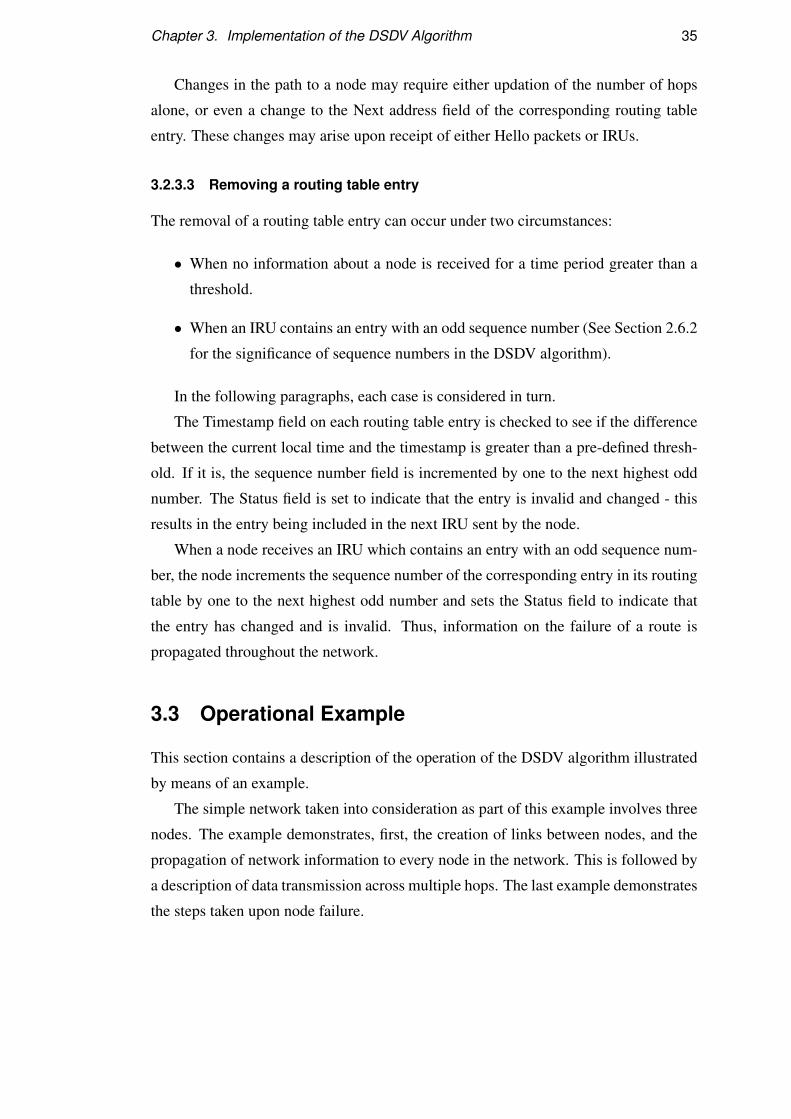
Chapter 3. Implementation of the DSDV Algorithm 35
Changes in the path to a node may require either updation of the number of hops
alone, or even a change to the Next address field of the corresponding routing table
entry. These changes may arise upon receipt of either Hello packets or IRUs.
3.2.3.3 Removing a routing table entry
The removal of a routing table entry can occur under two circumstances:
• When no information about a node is received for a time period greater than a
threshold.
• When an IRU contains an entry with an odd sequence number (See Section 2.6.2
for the significance of sequence numbers in the DSDV algorithm).
In the following paragraphs, each case is considered in turn.
The Timestamp field on each routing table entry is checked to see if the difference
between the current local time and the timestamp is greater than a pre-defined thresh-
old. If it is, the sequence number field is incremented by one to the next highest odd
number. The Status field is set to indicate that the entry is invalid and changed - this
results in the entry being included in the next IRU sent by the node.
When a node receives an IRU which contains an entry with an odd sequence num-
ber, the node increments the sequence number of the corresponding entry in its routing
table by one to the next highest odd number and sets the Status field to indicate that
the entry has changed and is invalid. Thus, information on the failure of a route is
propagated throughout the network.
3.3 Operational Example
This section contains a description of the operation of the DSDV algorithm illustrated
by means of an example.
The simple network taken into consideration as part of this example involves three
nodes. The example demonstrates, first, the creation of links between nodes, and the
propagation of network information to every node in the network. This is followed by
a description of data transmission across multiple hops. The last example demonstrates
the steps taken upon node failure.
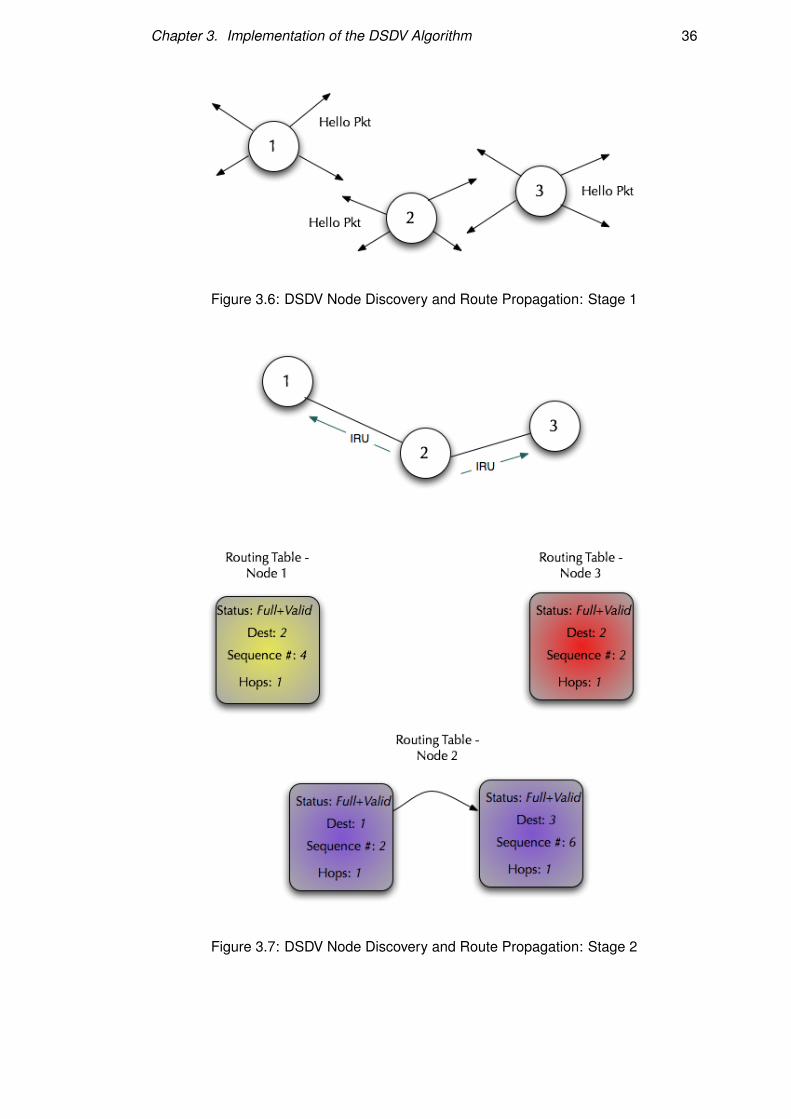
Chapter 3. Implementation of the DSDV Algorithm 36
Figure 3.6: DSDV Node Discovery and Route Propagation: Stage 1
Figure 3.7: DSDV Node Discovery and Route Propagation: Stage 2
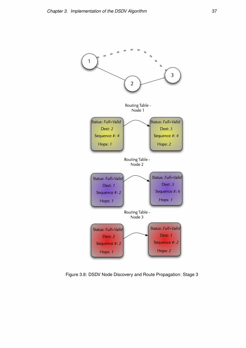
Chapter 3. Implementation of the DSDV Algorithm 37
Figure 3.8: DSDV Node Discovery and Route Propagation: Stage 3
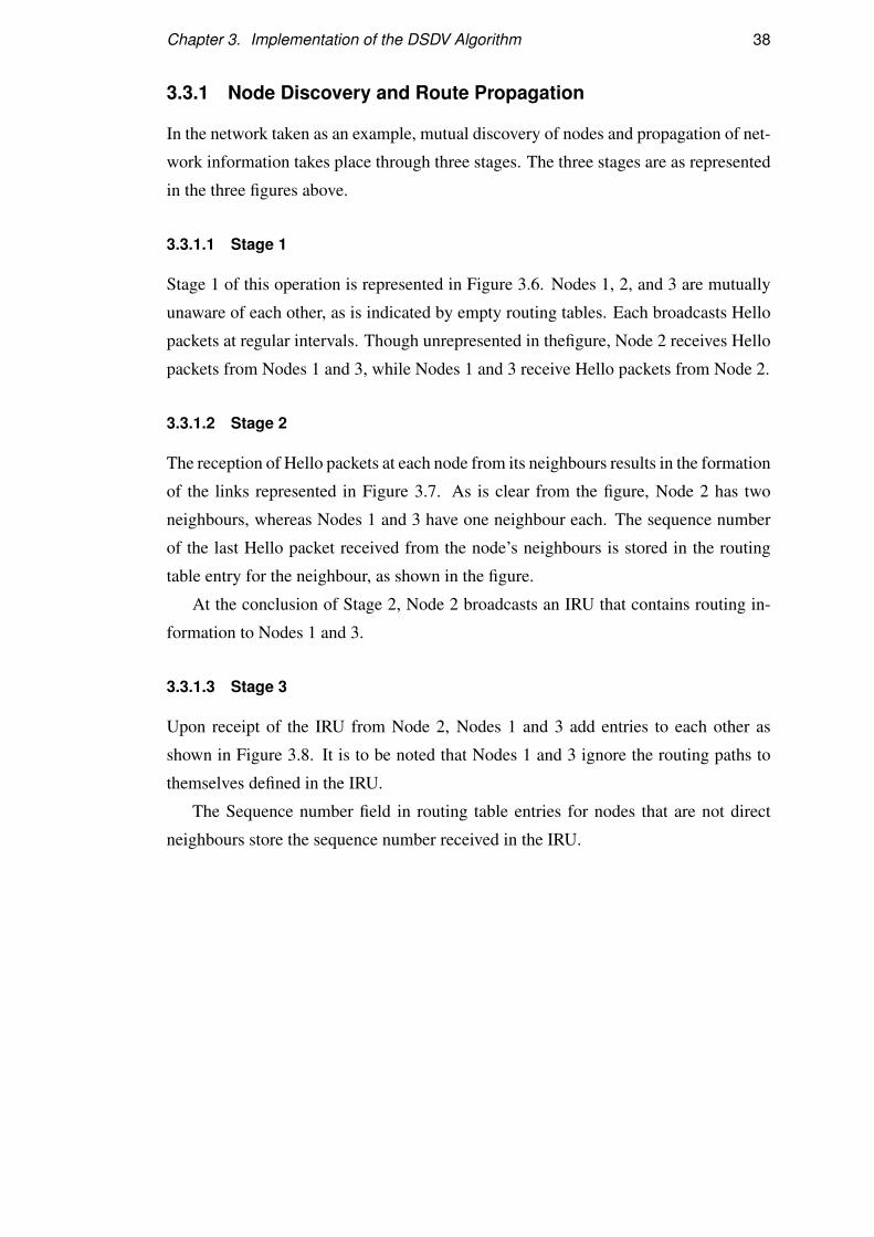
Chapter 3. Implementation of the DSDV Algorithm 38
3.3.1 Node Discovery and Route Propagation
In the network taken as an example, mutual discovery of nodes and propagation of net-
work information takes place through three stages. The three stages are as represented
in the three figures above.
3.3.1.1 Stage 1
Stage 1 of this operation is represented in Figure 3.6. Nodes 1, 2, and 3 are mutually
unaware of each other, as is indicated by empty routing tables. Each broadcasts Hello
packets at regular intervals. Though unrepresented in thefigure, Node 2 receives Hello
packets from Nodes 1 and 3, while Nodes 1 and 3 receive Hello packets from Node 2.
3.3.1.2 Stage 2
The reception of Hello packets at each node from its neighbours results in the formation
of the links represented in Figure 3.7. As is clear from the figure, Node 2 has two
neighbours, whereas Nodes 1 and 3 have one neighbour each. The sequence number
of the last Hello packet received from the node’s neighbours is stored in the routing
table entry for the neighbour, as shown in the figure.
At the conclusion of Stage 2, Node 2 broadcasts an IRU that contains routing in-
formation to Nodes 1 and 3.
3.3.1.3 Stage 3
Upon receipt of the IRU from Node 2, Nodes 1 and 3 add entries to each other as
shown in Figure 3.8. It is to be noted that Nodes 1 and 3 ignore the routing paths to
themselves defined in the IRU.
The Sequence number field in routing table entries for nodes that are not direct
neighbours store the sequence number received in the IRU.
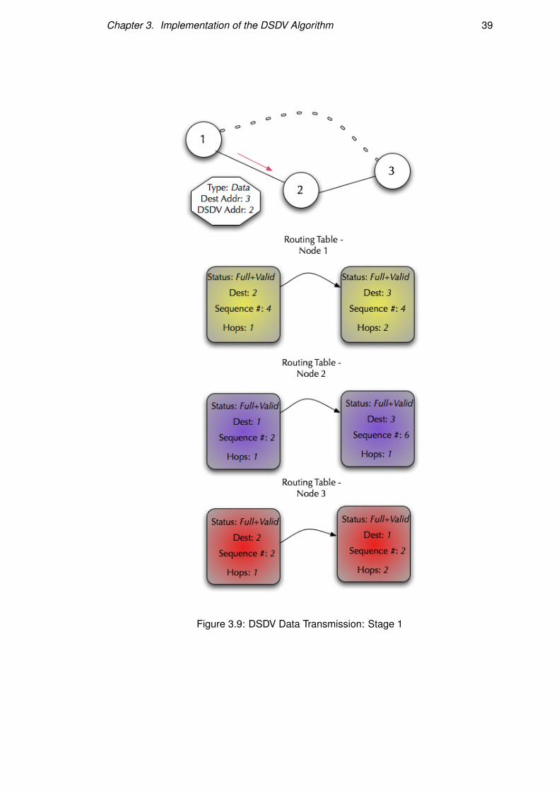
Chapter 3. Implementation of the DSDV Algorithm 39
Figure 3.9: DSDV Data Transmission: Stage 1
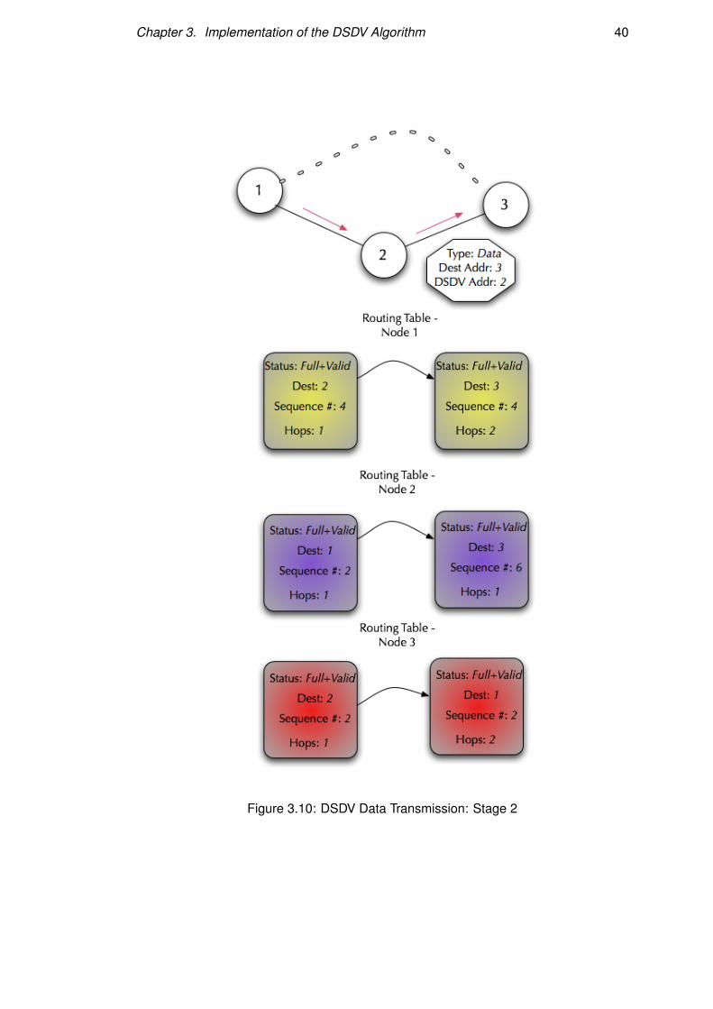
Chapter 3. Implementation of the DSDV Algorithm 40
Figure 3.10: DSDV Data Transmission: Stage 2
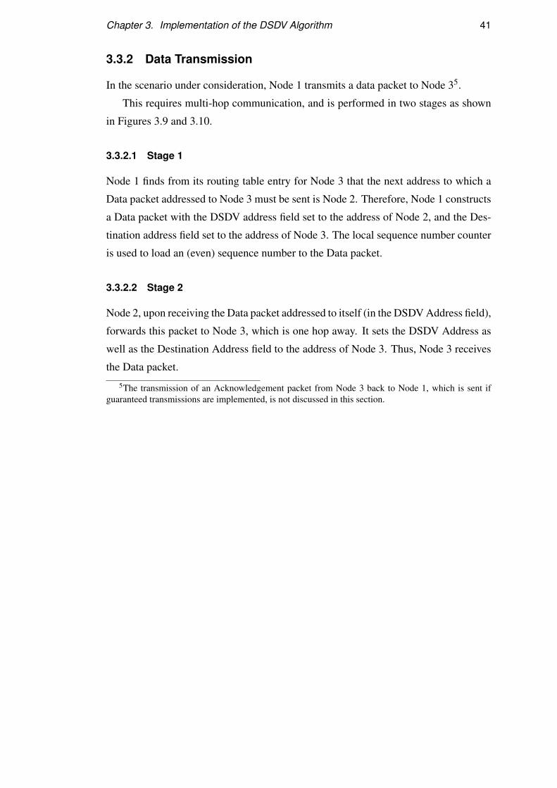
Chapter 3. Implementation of the DSDV Algorithm 41
3.3.2 Data Transmission
In the scenario under consideration, Node 1 transmits a data packet to Node 35.
This requires multi-hop communication, and is performed in two stages as shown
in Figures 3.9 and 3.10.
3.3.2.1 Stage 1
Node 1 finds from its routing table entry for Node 3 that the next address to which a
Data packet addressed to Node 3 must be sent is Node 2. Therefore, Node 1 constructs
a Data packet with the DSDV address field set to the address of Node 2, and the Des-
tination address field set to the address of Node 3. The local sequence number counter
is used to load an (even) sequence number to the Data packet.
3.3.2.2 Stage 2
Node 2, upon receiving the Data packet addressed to itself (in the DSDV Address field),
forwards this packet to Node 3, which is one hop away. It sets the DSDV Address as
well as the Destination Address field to the address of Node 3. Thus, Node 3 receives
the Data packet.
5The transmission of an Acknowledgement packet from Node 3 back to Node 1, which is sent ifguaranteed transmissions are implemented, is not discussed in this section.
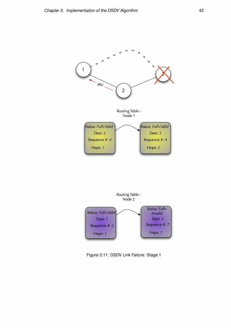
Chapter 3. Implementation of the DSDV Algorithm 42
Figure 3.11: DSDV Link Failure: Stage 1
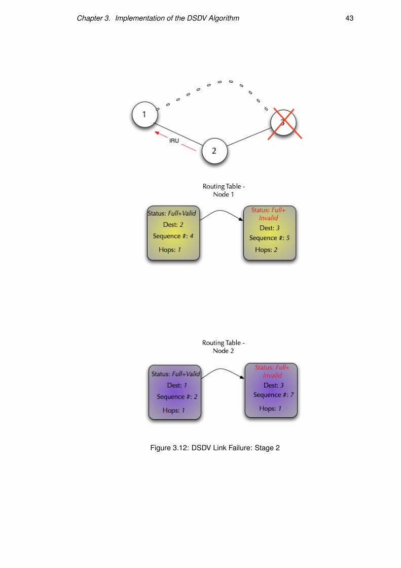
Chapter 3. Implementation of the DSDV Algorithm 43
Figure 3.12: DSDV Link Failure: Stage 2
Chapter 3. Implementation of the DSDV Algorithm 44
3.3.3 Link Failure
In this subsection, the example considers the failure of Node 3. This is a two stage
process as represented in Figures 3.11 and 3.12.
3.3.3.1 Stage 1
Node 2 realises the failure of Node 3 due to timer expiration. It then sets the status of
the routing table entry for Node 3 to indicate that the entry is invalid (and should not be
used to forward packets), and increments the sequence number field by one to the next
highest odd number. It then marks the routing table entry as changed, and broadcasts
the changed routing table entry in the next IRU it sends.
3.3.3.2 Stage 2
When Node 1 receives the IRU from Node 2, it notices that the entry for Node 3 in
the IRU sent has a higher odd sequence number. Therefore, it updates its routing table
entry for Node 3 to reflect the failure of Node 3. It then broadcasts this information in
the next IRU it sends.
3.4 Summary
This chapter opened with a short description of the position of the DSDV implemen-
tation in the protocol stack. The next section described the MAC layer primitives and
data structures used in the network layer, packet types defined in the network layer,
and a description of the structure of the routing table. The final section demonstrated
the operation of the DSDV algorithm with the help of an example.
Chapter 4
Applications using the DSDV
Algorithm - Visitor Tracking System
This chapter discusses an application implemented on the application layer atop the
DSDV algorithm discussed in the previous chapters. The motivation behind this appli-
cation - apart from the utility of the idea itself - was to investigate whether applications
for WSNs that could use MANET algorithms exist.
We begin with a discussion of the aims of the application, which is followed by a
brief presentation of the requirements of the VTS.
The next section describes the development environment, positions the VTS in the
protocol stack described in Section 3.1, discusses the top-level design of the application
layer, and concludes with a description of the packet types defined in the application
layer.
The final section of the chapter contains an exemplary description of the operation
of the application, which is followed, as always, by a short summary of the chapter
itself.
4.1 Aim
It is sometimes necessary to locate people and prevent their movement to restricted
or dangerous areas in small built-in environments. Human surveillance may be in-
sufficient to ensure this, and the consequences of failing to prevent human movement
to restricted areas can be potentially disastrous, especially if the humans involved are
young.
The purpose of this application was to design, using Specks (4), a Visitor Tracking
45
Chapter 4. Applications using the DSDV Algorithm - Visitor Tracking System 46
System, referred to henceforth as the VTS, which would provide a monitoring agent
such as a security guard or a nursery teacher with information on the position and the
direction of motion of visitors under their watch, and warnings if any visitors tried to
move to restricted areas.
It is our belief that this application can, with slight modifications, be applied to
several different domains.
4.2 Requirements
At the outset, the following requirements were outlined for the VTS:
• There are three kinds of nodes - Visitor Nodes (VN), Infrastructure Nodes (IN),
and Monitor Nodes (MN).
• The VNs and the MN must be mobile.
• The INs are fixed.
• The VNs must be lightweight and power-efficient. This necessitates a simple
VN design.
• The INs can be powered by a larger (possibly even AC) source as they are not
intended to be carried on a person. However, this also implies that they cannot
be frequently recharged.
• Since the monitoring agent, and thus by extension the MN, is the nerve-centre
of the VTS, the MN’s architecture will have to be relatively complex. However,
it can be recharged more frequently than the INs.
• Both the location and the direction of the motion of the VNs will have to be kept
track of.
4.3 Architecture
This section presents a brief description of the hardware and software platform upon
which the application was built, followed by a detailed presentation of the architecture
used.
Chapter 4. Applications using the DSDV Algorithm - Visitor Tracking System 47
4.3.1 Hardware and Software Platforms
This application was built on the Prospeckz IIK (4) hardware platform presented in
Section 2.2.2. The PSoC Designer IDE (29) was used to facilitate the development of
the system.
The SpeckMAC (38) algorithm described in Section 2.4 was used in the MAC
Layer, and the modified implementation of the DSDV algorithm presented in Chapter
3 was used in the network layer.
4.3.2 Protocol Stack
The protocol stack of the VTS application builds upon the one used in our implementa-
tion of the DSDV algorithm (see Section 3.1). New packet types - namely Ping, Pong,
and Visitor Information (VI) Packets - are defined in the VTS.
The DSDV algorithm in the network layer is used to construct a network of INs
and provide the sending and receiving primitives used by the application layer. This
section does not discuss the lower layers of the protocol stack. The protocol stack is
represented as shown in Figure 4.1.
4.3.3 The VTS in the Application Layer
In this section, we discuss the architecture of the three different node types used in the
VTS in some detail.
4.3.3.1 VN Architecture
The architecture of the VN is the simplest of the three. It continuously polls the receive
buffer for Ping packets sent by the INs and MN. If a Ping packet is received and the
VN is not currently attached to any node, it attaches itself to the sender of the Ping
packet, and records the transmission strength at which the Ping packet was sent1. The
VN then begins to send Pong packets addressed to the node that it received the Ping
packet from. The state information that the VN maintains is as shown below.
• Attached To: The IN/MN that the VN is currently attached to.
• Transmission Strength: The transmission strength at which the VN is attached to
the IN/MN.1The transmission strength, which is a 1 byte value ranging from 1 to 31, is stored in the data field
of the Ping packet sent.
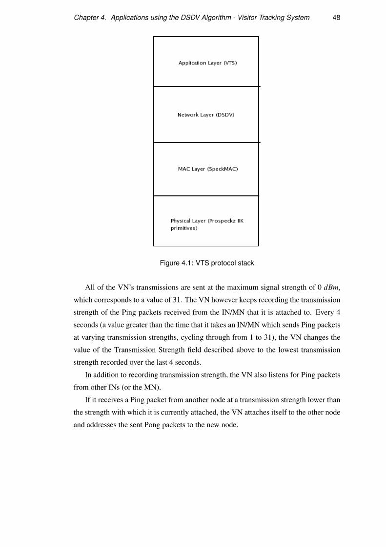
Chapter 4. Applications using the DSDV Algorithm - Visitor Tracking System 48
Figure 4.1: VTS protocol stack
All of the VN’s transmissions are sent at the maximum signal strength of 0 dBm,
which corresponds to a value of 31. The VN however keeps recording the transmission
strength of the Ping packets received from the IN/MN that it is attached to. Every 4
seconds (a value greater than the time that it takes an IN/MN which sends Ping packets
at varying transmission strengths, cycling through from 1 to 31), the VN changes the
value of the Transmission Strength field described above to the lowest transmission
strength recorded over the last 4 seconds.
In addition to recording transmission strength, the VN also listens for Ping packets
from other INs (or the MN).
If it receives a Ping packet from another node at a transmission strength lower than
the strength with which it is currently attached, the VN attaches itself to the other node
and addresses the sent Pong packets to the new node.
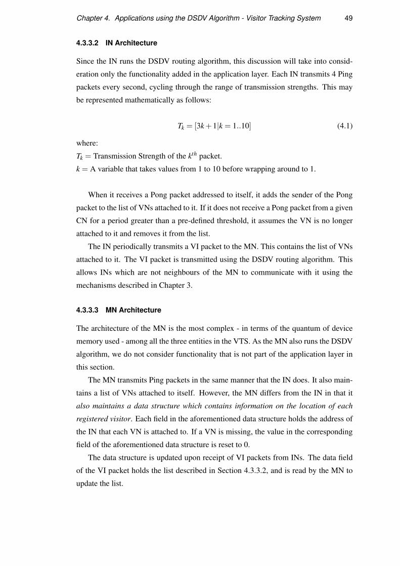
Chapter 4. Applications using the DSDV Algorithm - Visitor Tracking System 49
4.3.3.2 IN Architecture
Since the IN runs the DSDV routing algorithm, this discussion will take into consid-
eration only the functionality added in the application layer. Each IN transmits 4 Ping
packets every second, cycling through the range of transmission strengths. This may
be represented mathematically as follows:
Tk = [3k +1|k = 1..10] (4.1)
where:
Tk = Transmission Strength of the kth packet.
k = A variable that takes values from 1 to 10 before wrapping around to 1.
When it receives a Pong packet addressed to itself, it adds the sender of the Pong
packet to the list of VNs attached to it. If it does not receive a Pong packet from a given
CN for a period greater than a pre-defined threshold, it assumes the VN is no longer
attached to it and removes it from the list.
The IN periodically transmits a VI packet to the MN. This contains the list of VNs
attached to it. The VI packet is transmitted using the DSDV routing algorithm. This
allows INs which are not neighbours of the MN to communicate with it using the
mechanisms described in Chapter 3.
4.3.3.3 MN Architecture
The architecture of the MN is the most complex - in terms of the quantum of device
memory used - among all the three entities in the VTS. As the MN also runs the DSDV
algorithm, we do not consider functionality that is not part of the application layer in
this section.
The MN transmits Ping packets in the same manner that the IN does. It also main-
tains a list of VNs attached to itself. However, the MN differs from the IN in that it
also maintains a data structure which contains information on the location of each
registered visitor. Each field in the aforementioned data structure holds the address of
the IN that each VN is attached to. If a VN is missing, the value in the corresponding
field of the aforementioned data structure is reset to 0.
The data structure is updated upon receipt of VI packets from INs. The data field
of the VI packet holds the list described in Section 4.3.3.2, and is read by the MN to
update the list.

Chapter 4. Applications using the DSDV Algorithm - Visitor Tracking System 50
Figure 4.2: VTS packet types
Bit Bit 15 = 1 Bit 15 = 0
14 Hello Packet Ping Packet
13 Incremental Routing Update Pong Packet
12 – Visitor Information Packet
Table 4.1: VTS Packet type identifiers
The MN periodically updates the user display - which may be on a PDA or a PC -
using the UART.
4.3.4 Packet Types in the Application Layer
This section contains a brief overview of the packet types defined in the application
layer. These packets were introduced in the previous section.
The packet types available in the VTS application are shown in Figure 4.2. Packet
types used only by VNs are represented in black, packet types used by the INs and the
MN in blue, and packet types used only by INs in red.
The packet type identifiers are specified according to Table 4.1 (please note that
Protocol packets have the same identifiers as described in Table 3.1 in Chapter 3). As
is clear from the table , the packet types defined in the application layer are subtypes
of data packets, as far as the DSDV implementation in the network layer is concerned.
4.3.4.1 Ping packets
Ping packets are sent both by the MN and the INs. Four of these packets are transmitted
every second as described in Section 4.3.3.2. The sequence of transmission strengths
chosen may be mathematically represented as shown in Equation 4.1. The Ping packets
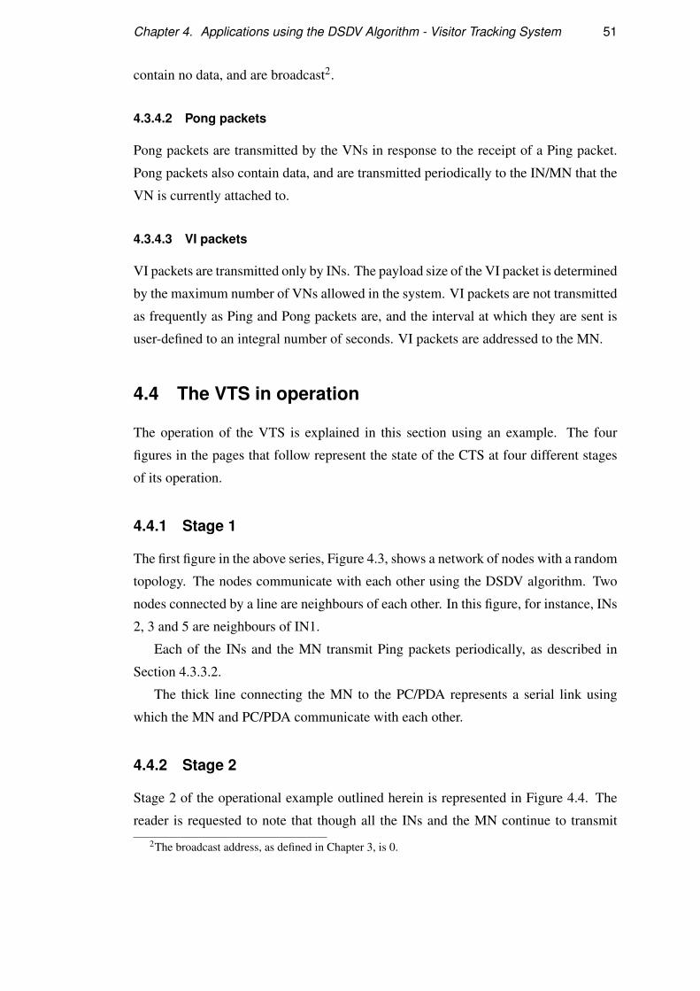
Chapter 4. Applications using the DSDV Algorithm - Visitor Tracking System 51
contain no data, and are broadcast2.
4.3.4.2 Pong packets
Pong packets are transmitted by the VNs in response to the receipt of a Ping packet.
Pong packets also contain data, and are transmitted periodically to the IN/MN that the
VN is currently attached to.
4.3.4.3 VI packets
VI packets are transmitted only by INs. The payload size of the VI packet is determined
by the maximum number of VNs allowed in the system. VI packets are not transmitted
as frequently as Ping and Pong packets are, and the interval at which they are sent is
user-defined to an integral number of seconds. VI packets are addressed to the MN.
4.4 The VTS in operation
The operation of the VTS is explained in this section using an example. The four
figures in the pages that follow represent the state of the CTS at four different stages
of its operation.
4.4.1 Stage 1
The first figure in the above series, Figure 4.3, shows a network of nodes with a random
topology. The nodes communicate with each other using the DSDV algorithm. Two
nodes connected by a line are neighbours of each other. In this figure, for instance, INs
2, 3 and 5 are neighbours of IN1.
Each of the INs and the MN transmit Ping packets periodically, as described in
Section 4.3.3.2.
The thick line connecting the MN to the PC/PDA represents a serial link using
which the MN and PC/PDA communicate with each other.
4.4.2 Stage 2
Stage 2 of the operational example outlined herein is represented in Figure 4.4. The
reader is requested to note that though all the INs and the MN continue to transmit
2The broadcast address, as defined in Chapter 3, is 0.
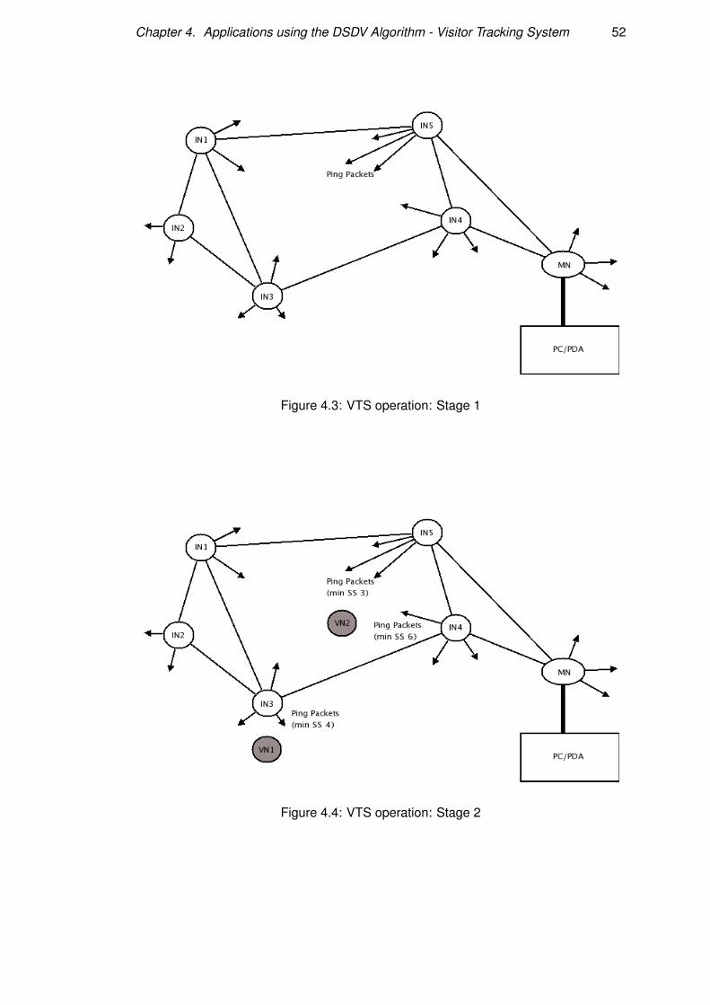
Chapter 4. Applications using the DSDV Algorithm - Visitor Tracking System 52
Figure 4.3: VTS operation: Stage 1
Figure 4.4: VTS operation: Stage 2
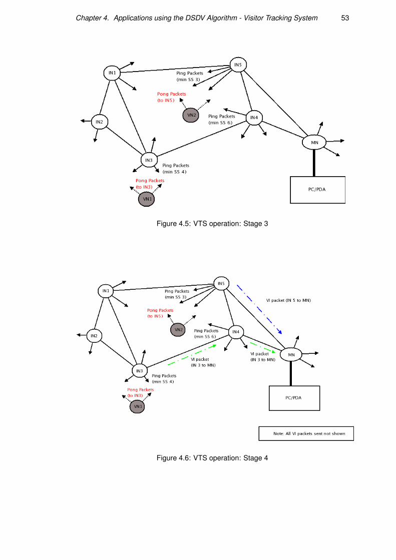
Chapter 4. Applications using the DSDV Algorithm - Visitor Tracking System 53
Figure 4.5: VTS operation: Stage 3
Figure 4.6: VTS operation: Stage 4
Chapter 4. Applications using the DSDV Algorithm - Visitor Tracking System 54
Ping packets, only the transmissions of INs 3, 4, and 5 are represented3.
VN1 receives only those Ping packets that are sent by IN3. Therefore, it attaches
itself to IN3 at the lowest received signal strength; which in this case is 4.
VN2, on the other hand, receives Ping packets from INs 4 and 5. The weakest
signal strength that it receives from IN4 is 5, whereas it receives a Ping packet at a
(minimum) signal strength of 3 from IN5. As a result of this, VN2 attaches itself to
IN5.
4.4.3 Stage 3
Figure 4.5 represents the third stage of this example, and models post-attachment VN
behaviour. Both VNs 1 and 2 begin transmitting Pong packets addressed to INs 3
and 5 respectively. Upon receipt of the Pong packets, INs 3 and 5 add VNs 1 and 2
respectively to their lists of attached VNs.
4.4.4 Stage 4
The final stage of operation (see Figure 4.6) involves the communication of VN loca-
tion information to the MN, which in turn communicates it to the PDA.
When INs 3 and 5 next send a VI packet to the MN, the attachment information -
discovered in the previous stage of operation described here - is sent. The MN then
collates this information, and communicates it to the monitoring agent’s PC/PDA over
the serial link. The PC/PDA renders the received data on screen.
Referring to Figure 4.6, the reader is requested to note that:
• The green dotted lines represent the VI packet(s) sent from IN3 to the MN. This
transfer is multi-hop, and uses the DSDV algorithm.
• The red dotted lines represent the VI packet(s) sent from IN5 to the MN, which
is its direct neighbour.
• All INs send VI packets to the MN. However, to enhance the readability of the
diagram, they are not shown.
• The network has no form of global synchronisation. Therefore, each IN sends
VI packets at different times. Additionally, the intervals between successive VI
3This is done in order to enhance readability.
Chapter 4. Applications using the DSDV Algorithm - Visitor Tracking System 55
packets may vary from node to node and may change within a node over the
course of operation as a result of clock drift.
4.5 Summary
This chapter started with the definition of the aim of the VTS application, and was
followed by a short outline of the requirements for the application. The next section
presented the architecture of the application; including the hardware and software plat-
form used, the position of the VTS in the protocol stack, and the packet types used in
the VTS. The final section included an exemplary description of the operation of the
VTS.
Chapter 5
Implementation of the ZRP Algorithm
This chapter presents the implementation of the ZRP algorithm (15) on the Prospeckz
IIK.
In the first section, the protocol stack within which the ZRP implementation resides
is presented. This is followed by a description of the differences between the DSDV
implementation discussed in Chapter 3 and that used for intra-zone communication in
the ZRP implementation. The final section discusses the data structures used by the
reactive algorithm used to facilitate inter-zone communication - namely, the packet
formats, route discovery protocol, and route caching mechanisms. The chapter con-
cludes after elucidating the operation of the ZRP algorithm using an example that lays
emphasis on the inter-zone route discovery protocol.
5.1 Protocol Stack
Figure 5.1 summarises the protocol stack within which the implementation of the ZRP
algorithm resides.
The protocol stack is similar to that used with the DSDV implementation described
in Chapter 3. The ZRP algorithm is developed on the Prospeckz IIK (4) described in
Section 2.2.2, and uses the SpeckMAC-D (38) algorithm, referred to henceforth as the
SpeckMAC algorithm, in the MAC layer1.
The ZRP implementation also uses, just as the DSDV implementation does, the
sending and receiving primitives and packet formats defined in the SpeckMAC algo-
rithm. The discussion of the lower-level primitives is not repeated in this chapter.
1The SpeckMAC-D variant was chosen over SpeckMAC-B because (38) indicates that it performsbetter.
56
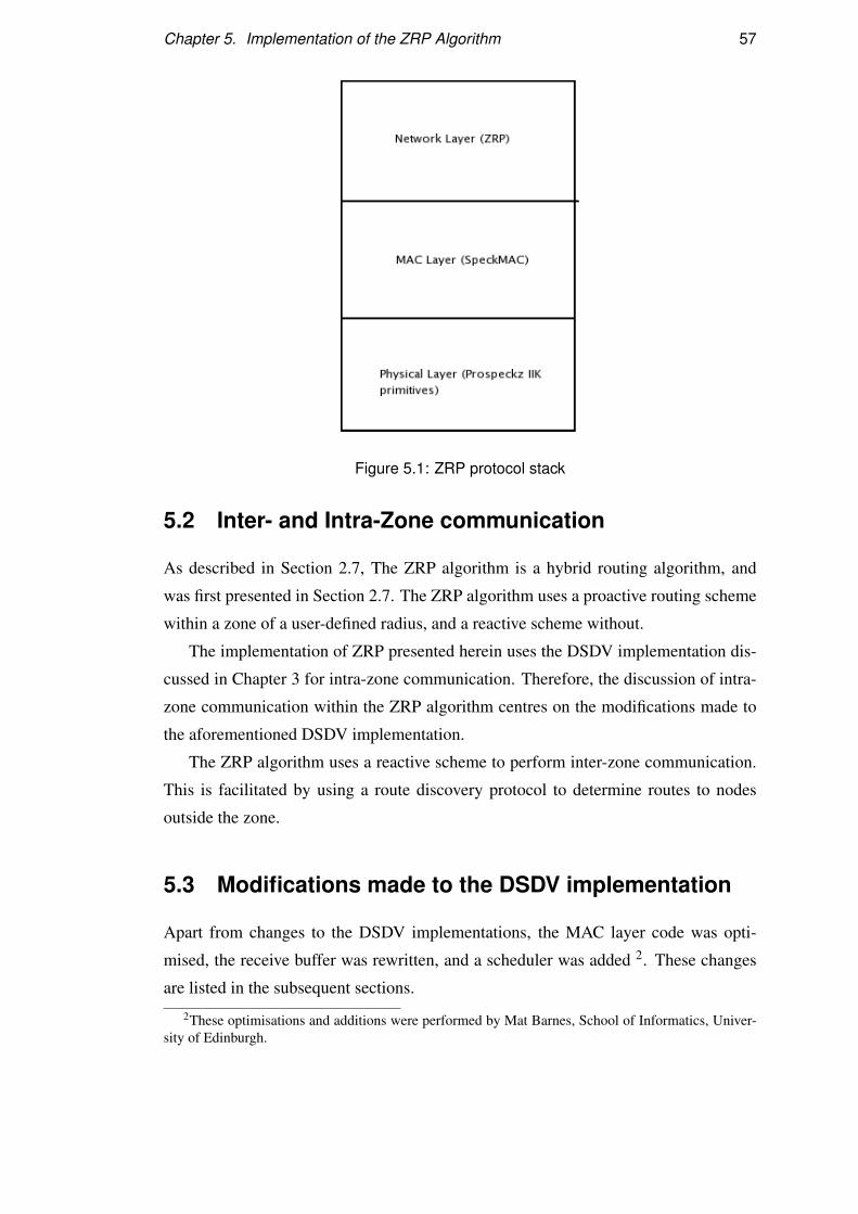
Chapter 5. Implementation of the ZRP Algorithm 57
Figure 5.1: ZRP protocol stack
5.2 Inter- and Intra-Zone communication
As described in Section 2.7, The ZRP algorithm is a hybrid routing algorithm, and
was first presented in Section 2.7. The ZRP algorithm uses a proactive routing scheme
within a zone of a user-defined radius, and a reactive scheme without.
The implementation of ZRP presented herein uses the DSDV implementation dis-
cussed in Chapter 3 for intra-zone communication. Therefore, the discussion of intra-
zone communication within the ZRP algorithm centres on the modifications made to
the aforementioned DSDV implementation.
The ZRP algorithm uses a reactive scheme to perform inter-zone communication.
This is facilitated by using a route discovery protocol to determine routes to nodes
outside the zone.
5.3 Modifications made to the DSDV implementation
Apart from changes to the DSDV implementations, the MAC layer code was opti-
mised, the receive buffer was rewritten, and a scheduler was added 2. These changes
are listed in the subsequent sections.
2These optimisations and additions were performed by Mat Barnes, School of Informatics, Univer-sity of Edinburgh.
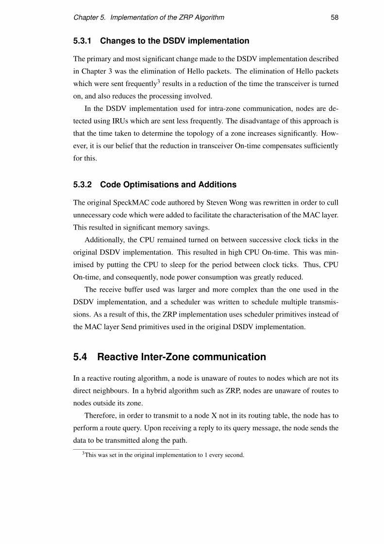
Chapter 5. Implementation of the ZRP Algorithm 58
5.3.1 Changes to the DSDV implementation
The primary and most significant change made to the DSDV implementation described
in Chapter 3 was the elimination of Hello packets. The elimination of Hello packets
which were sent frequently3 results in a reduction of the time the transceiver is turned
on, and also reduces the processing involved.
In the DSDV implementation used for intra-zone communication, nodes are de-
tected using IRUs which are sent less frequently. The disadvantage of this approach is
that the time taken to determine the topology of a zone increases significantly. How-
ever, it is our belief that the reduction in transceiver On-time compensates sufficiently
for this.
5.3.2 Code Optimisations and Additions
The original SpeckMAC code authored by Steven Wong was rewritten in order to cull
unnecessary code which were added to facilitate the characterisation of the MAC layer.
This resulted in significant memory savings.
Additionally, the CPU remained turned on between successive clock ticks in the
original DSDV implementation. This resulted in high CPU On-time. This was min-
imised by putting the CPU to sleep for the period between clock ticks. Thus, CPU
On-time, and consequently, node power consumption was greatly reduced.
The receive buffer used was larger and more complex than the one used in the
DSDV implementation, and a scheduler was written to schedule multiple transmis-
sions. As a result of this, the ZRP implementation uses scheduler primitives instead of
the MAC layer Send primitives used in the original DSDV implementation.
5.4 Reactive Inter-Zone communication
In a reactive routing algorithm, a node is unaware of routes to nodes which are not its
direct neighbours. In a hybrid algorithm such as ZRP, nodes are unaware of routes to
nodes outside its zone.
Therefore, in order to transmit to a node X not in its routing table, the node has to
perform a route query. Upon receiving a reply to its query message, the node sends the
data to be transmitted along the path.
3This was set in the original implementation to 1 every second.
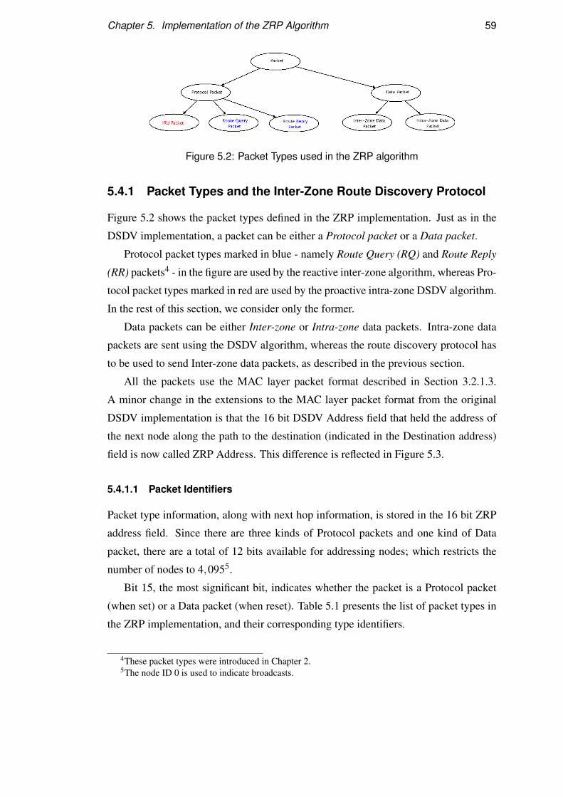
Chapter 5. Implementation of the ZRP Algorithm 59
Figure 5.2: Packet Types used in the ZRP algorithm
5.4.1 Packet Types and the Inter-Zone Route Discovery Protocol
Figure 5.2 shows the packet types defined in the ZRP implementation. Just as in the
DSDV implementation, a packet can be either a Protocol packet or a Data packet.
Protocol packet types marked in blue - namely Route Query (RQ) and Route Reply
(RR) packets4 - in the figure are used by the reactive inter-zone algorithm, whereas Pro-
tocol packet types marked in red are used by the proactive intra-zone DSDV algorithm.
In the rest of this section, we consider only the former.
Data packets can be either Inter-zone or Intra-zone data packets. Intra-zone data
packets are sent using the DSDV algorithm, whereas the route discovery protocol has
to be used to send Inter-zone data packets, as described in the previous section.
All the packets use the MAC layer packet format described in Section 3.2.1.3.
A minor change in the extensions to the MAC layer packet format from the original
DSDV implementation is that the 16 bit DSDV Address field that held the address of
the next node along the path to the destination (indicated in the Destination address)
field is now called ZRP Address. This difference is reflected in Figure 5.3.
5.4.1.1 Packet Identifiers
Packet type information, along with next hop information, is stored in the 16 bit ZRP
address field. Since there are three kinds of Protocol packets and one kind of Data
packet, there are a total of 12 bits available for addressing nodes; which restricts the
number of nodes to 4,0955.
Bit 15, the most significant bit, indicates whether the packet is a Protocol packet
(when set) or a Data packet (when reset). Table 5.1 presents the list of packet types in
the ZRP implementation, and their corresponding type identifiers.
4These packet types were introduced in Chapter 2.5The node ID 0 is used to indicate broadcasts.
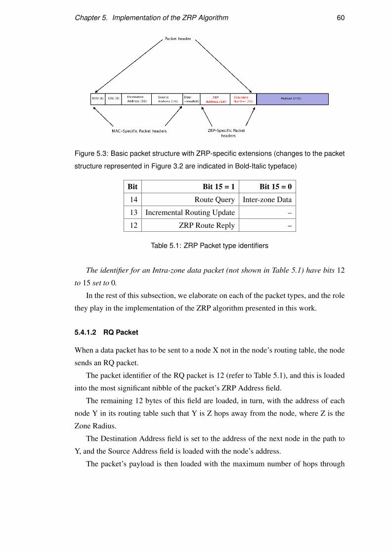
Chapter 5. Implementation of the ZRP Algorithm 60
Figure 5.3: Basic packet structure with ZRP-specific extensions (changes to the packet
structure represented in Figure 3.2 are indicated in Bold-Italic typeface)
Bit Bit 15 = 1 Bit 15 = 0
14 Route Query Inter-zone Data
13 Incremental Routing Update –
12 ZRP Route Reply –
Table 5.1: ZRP Packet type identifiers
The identifier for an Intra-zone data packet (not shown in Table 5.1) have bits 12
to 15 set to 0.
In the rest of this subsection, we elaborate on each of the packet types, and the role
they play in the implementation of the ZRP algorithm presented in this work.
5.4.1.2 RQ Packet
When a data packet has to be sent to a node X not in the node’s routing table, the node
sends an RQ packet.
The packet identifier of the RQ packet is 12 (refer to Table 5.1), and this is loaded
into the most significant nibble of the packet’s ZRP Address field.
The remaining 12 bytes of this field are loaded, in turn, with the address of each
node Y in its routing table such that Y is Z hops away from the node, where Z is the
Zone Radius.
The Destination Address field is set to the address of the next node in the path to
Y, and the Source Address field is loaded with the node’s address.
The packet’s payload is then loaded with the maximum number of hops through
Chapter 5. Implementation of the ZRP Algorithm 61
which the RQ packet is sent before it is discarded, the address of the node X, and the
current node’s address. This is done in order to (later) construct a path from the sender
to the receiver.
When a node receives an RQ packet, it checks to see if it is the final destination
node, or if there exists an entry for X in its routing table.
If either of the above conditions holds true, then the node sends an RR packet to
the querying node, the address of which is contained within the payload.
If not, the node decrements the Hop count field in the payload of the received RQ
packet by one. If the resulting value is equal to 0, the RQ packet is discarded.
If the Hop count is greater than 0, the node forwards the RQ packet to every node
in its zone radius, after adding its own address to the payload, and setting the Source
address field to the local address6.
5.4.1.3 RR Packet
An RR packet is sent when a node receives a RQ packet that is searching for a path
either to the node itself or to another node in the node’s routing table.
An RR packet has an identifier of 9, which is loaded into the most significant nibble
of the packet’s ZRP address field. The Destination address field is set to the previous
node along the path taken by the query message. This is extracted from the payload of
the received RQ packet. The Source address field is set to the local address.
The path to the queried destination is then loaded into the payload. If the node
sending the reply message is the queried destination, then it merely adds its address to
the path. If, on the other hand, the queried destination is in the node’s routing table, it
adds its local address and the next address on the path to the queried destination.
Each node that receives an RR packet checks to discover its position in the path
back to the source, and forwards the packet along this path.
This exchange of RQ and RR packets in order to discover the path to a destination
constitutes the Inter-zone Route Discovery Protocol.
5.4.1.4 Intra-zone Data Packet
Intra-zone Data packets are used to transmit data within a zone. They are routed using
the DSDV algorithm.
6It is worth noting at this point that the RQ packet is not sent to nodes that have already been inreceipt of the packet.
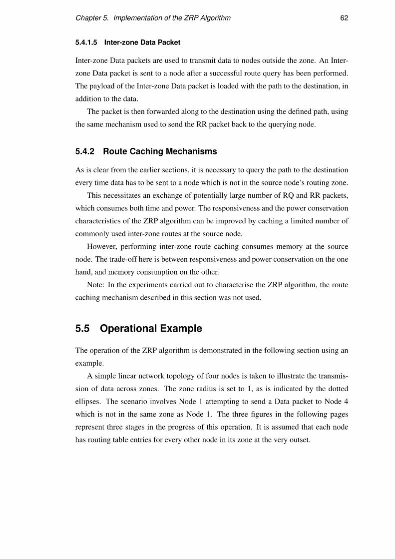
Chapter 5. Implementation of the ZRP Algorithm 62
5.4.1.5 Inter-zone Data Packet
Inter-zone Data packets are used to transmit data to nodes outside the zone. An Inter-
zone Data packet is sent to a node after a successful route query has been performed.
The payload of the Inter-zone Data packet is loaded with the path to the destination, in
addition to the data.
The packet is then forwarded along to the destination using the defined path, using
the same mechanism used to send the RR packet back to the querying node.
5.4.2 Route Caching Mechanisms
As is clear from the earlier sections, it is necessary to query the path to the destination
every time data has to be sent to a node which is not in the source node’s routing zone.
This necessitates an exchange of potentially large number of RQ and RR packets,
which consumes both time and power. The responsiveness and the power conservation
characteristics of the ZRP algorithm can be improved by caching a limited number of
commonly used inter-zone routes at the source node.
However, performing inter-zone route caching consumes memory at the source
node. The trade-off here is between responsiveness and power conservation on the one
hand, and memory consumption on the other.
Note: In the experiments carried out to characterise the ZRP algorithm, the route
caching mechanism described in this section was not used.
5.5 Operational Example
The operation of the ZRP algorithm is demonstrated in the following section using an
example.
A simple linear network topology of four nodes is taken to illustrate the transmis-
sion of data across zones. The zone radius is set to 1, as is indicated by the dotted
ellipses. The scenario involves Node 1 attempting to send a Data packet to Node 4
which is not in the same zone as Node 1. The three figures in the following pages
represent three stages in the progress of this operation. It is assumed that each node
has routing table entries for every other node in its zone at the very outset.
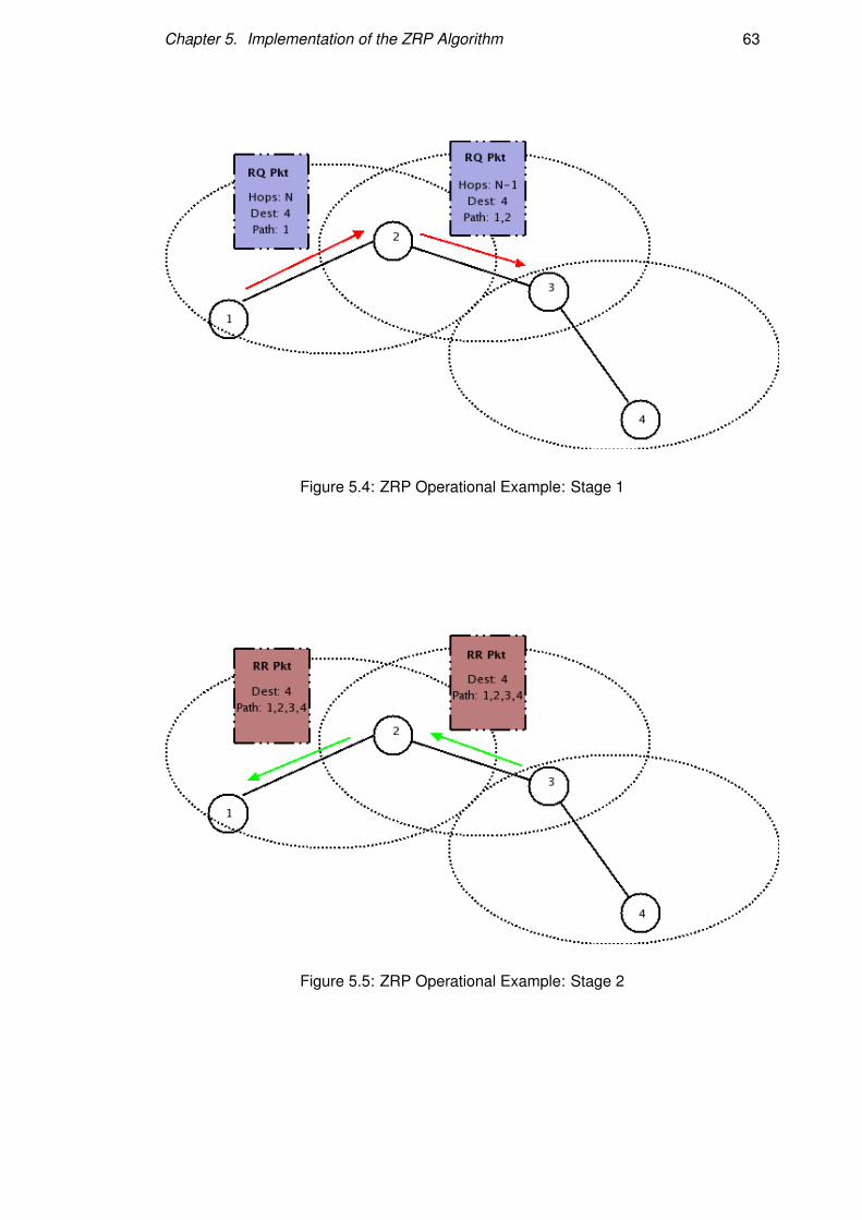
Chapter 5. Implementation of the ZRP Algorithm 63
Figure 5.4: ZRP Operational Example: Stage 1
Figure 5.5: ZRP Operational Example: Stage 2
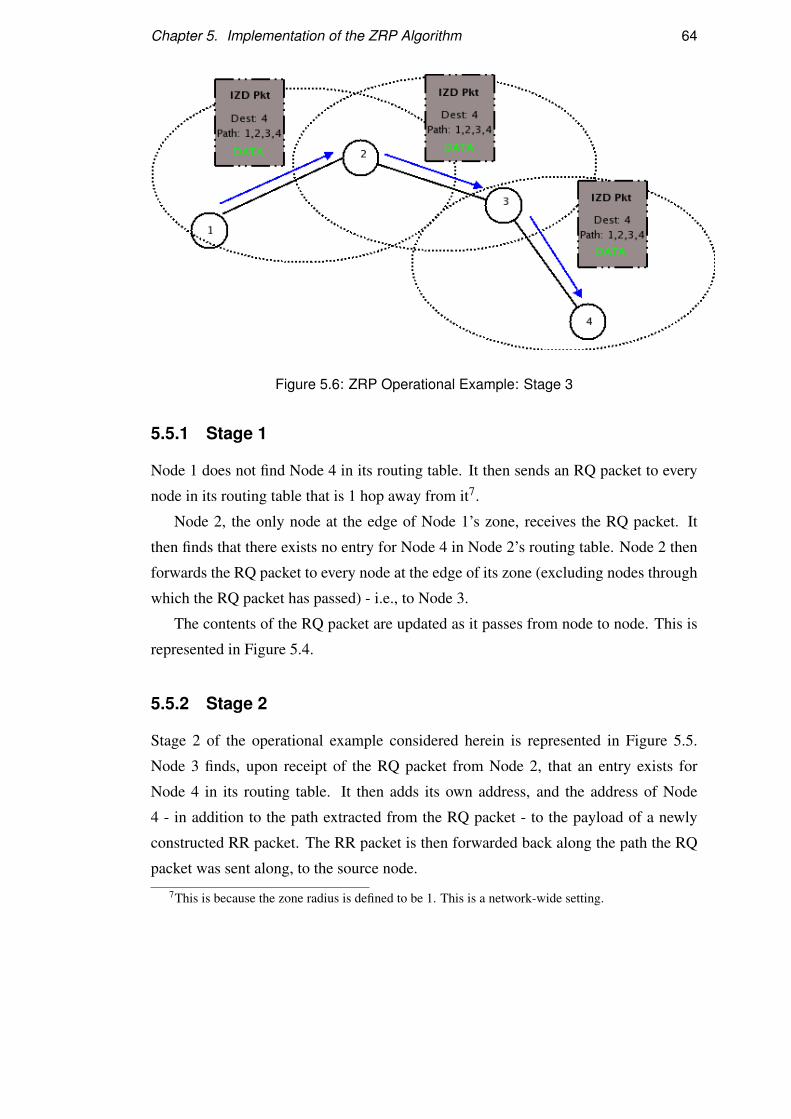
Chapter 5. Implementation of the ZRP Algorithm 64
Figure 5.6: ZRP Operational Example: Stage 3
5.5.1 Stage 1
Node 1 does not find Node 4 in its routing table. It then sends an RQ packet to every
node in its routing table that is 1 hop away from it7.
Node 2, the only node at the edge of Node 1’s zone, receives the RQ packet. It
then finds that there exists no entry for Node 4 in Node 2’s routing table. Node 2 then
forwards the RQ packet to every node at the edge of its zone (excluding nodes through
which the RQ packet has passed) - i.e., to Node 3.
The contents of the RQ packet are updated as it passes from node to node. This is
represented in Figure 5.4.
5.5.2 Stage 2
Stage 2 of the operational example considered herein is represented in Figure 5.5.
Node 3 finds, upon receipt of the RQ packet from Node 2, that an entry exists for
Node 4 in its routing table. It then adds its own address, and the address of Node
4 - in addition to the path extracted from the RQ packet - to the payload of a newly
constructed RR packet. The RR packet is then forwarded back along the path the RQ
packet was sent along, to the source node.
7This is because the zone radius is defined to be 1. This is a network-wide setting.
Chapter 5. Implementation of the ZRP Algorithm 65
5.5.3 Stage 3
Figure 5.6 represents the third stage of this example, and shows the actual transmission
of data from the source to the destination. The queried path to Node 4 is appended to
the data in the payload field of the Inter-zone Data packet. The packet is then forwarded
to Node 4 along the path specified in the payload field.
5.6 Summary
At the outset of this chapter, the structure of which was similar to that of the previous
chapter, the position of the ZRP implementation in the protocol stack was described.
This was followed by a discussion of the modifications made to the DSDV implemen-
tation and to the underlying code itself, and the implications of the same. The next
section then expounded on the implementation of reactive inter-zone communication
in considerable detail. The last section illustrated the operation of the ZRP algorithm
by means of an example.
The chapters that follow describe the experimental methodology used, and analyse
the results obtained upon measuring defined metrics on the implemented algorithms
and applications.
Chapter 6
Experimental Methodology
The discussion in this chapter centres on the experimental methodology used to char-
acterise the algorithms and applications developed as part of this thesis.
The first section presents the metrics chosen for characterisation of the algorithms
and applications considered in this work. Also described in this section are metrics
that were used for the analysis of the application implemented.
This is followed in the next section by a description of the measurement techniques
used for each of the metrics described in the first section. Additionally, attempts are
made to describe the slight differences between algorithms in the mechanisms used
to measure the different metrics. The chapter concludes with a short summary of the
metrics discussed during the course of the chapter.
Note: The differences between the implementation of the DSDV algorithm, and
the DSDV implementation used to facilitate intra-zone communication in the ZRP al-
gorithm were discussed in Chapter 5. Therefore, in order to facilitate comparison
between the ZRP and DSDV implementations, the analysis of the DSDV algorithm was
performed on the modified implementation1 used within the ZRP implementation.
6.1 Metrics Used for Characterisation
Three metrics were used to characterise the algorithms and applications developed
herein. Each of these metrics is elaborated on in the subsequent sections.
1This implementation also incorporates the optimisations described in Section 5.3.2.
66

Chapter 6. Experimental Methodology 67
6.1.1 Transmission Time
This metric was used to determine the time taken for a packet to be sent across multiple
hops using the algorithm. This time includes:
• The time required for the sender to discover the path to the receiver.
• The time required at the sender to construct the packet. This depends on the
processor and not on the radio transmission rate.
• The time that the node may need to wait for the medium to clear before the
packet is sent. This depends on the traffic in the medium; which in turn depends
on the number of nodes in the immediate vicinity and their rate of transmission.
• The time required to transmit the packet through to the destination. This depends
not just on the transmission rate of the CC2420 radio but also on the number of
intermediary nodes that need to receive the packet, process and modify it, and
retransmit it on to the next node on the path to the destination.
• The time required at the final destination to receive the packet, copy it into the
receive buffer, and for the packet to be retrieved from the receive buffer and
process it.
This metric was used to characterise both the DSDV (26) and the ZRP (15) routing
algorithms, but was not used to analyse the performance of the VTS application.
6.1.2 Delivery Ratio
The delivery ratio may be defined as the ratio of the number of packets sent by the
source node to the number of packets received at the destination node. The delivery
ratio depends on the number of hops across which the packet is sent, and the delivery
ratio of the MAC layer (namely, the SpeckMAC algorithm (38)).
6.1.3 Transmitter/Receiver On-time
Transmitter/Receiver (Tx/Rx) On-time may be defined as the proportion of the total
time for which the transmitter or receiver are turned on at a node that runs the al-
gorithm/application being characterised. It provides a measure, not of the efficiency
of the algorithm/application implemented, but that of the implementation of the algo-
rithm. However, this is a valuable metric for performing comparisons, and to analyse
Chapter 6. Experimental Methodology 68
the suitability of an algorithm/application for use in WSNs. The proportion of time
the transmitter/receiver is turned on may be directly related to the power consumption
characteristics.
6.1.4 Metrics used for application characterisation
The following metrics were used only to perform the characterisation of the applica-
tion, and not the algorithms implemented. This is because the results obtained upon
running experiments on these metrics depend on the efficiency of the implementation,
and not of the algorithm itself.
The metrics used for application characterisation are described in the following
subsections.
6.1.4.1 Average Current Consumption
The average current consumption is defined as the current consumed, on average, by
the application per unit time. This is determined by measuring the instantaneous cur-
rent consumption over a period of time.
6.1.4.2 Average Power Consumption
The power consumption is calculated from the average current consumption and the
voltage drawn by the node, and is hence dependent on the measure of current con-
sumption.
6.1.4.3 CPU On-time
The CPU On-time is defined as the proportion of time for which the Central Processing
Unit (CPU) of the node running the application is turned on. It is a ratio of the time
the CPU stayed on to the time the application is running.
6.2 Measurement Techniques
The experimental setup used to measure each of the metrics described in the previous
section are discussed here. Additionally, the differences (if any) in the methods used
to measure the same metric for different algorithms are also outlined.
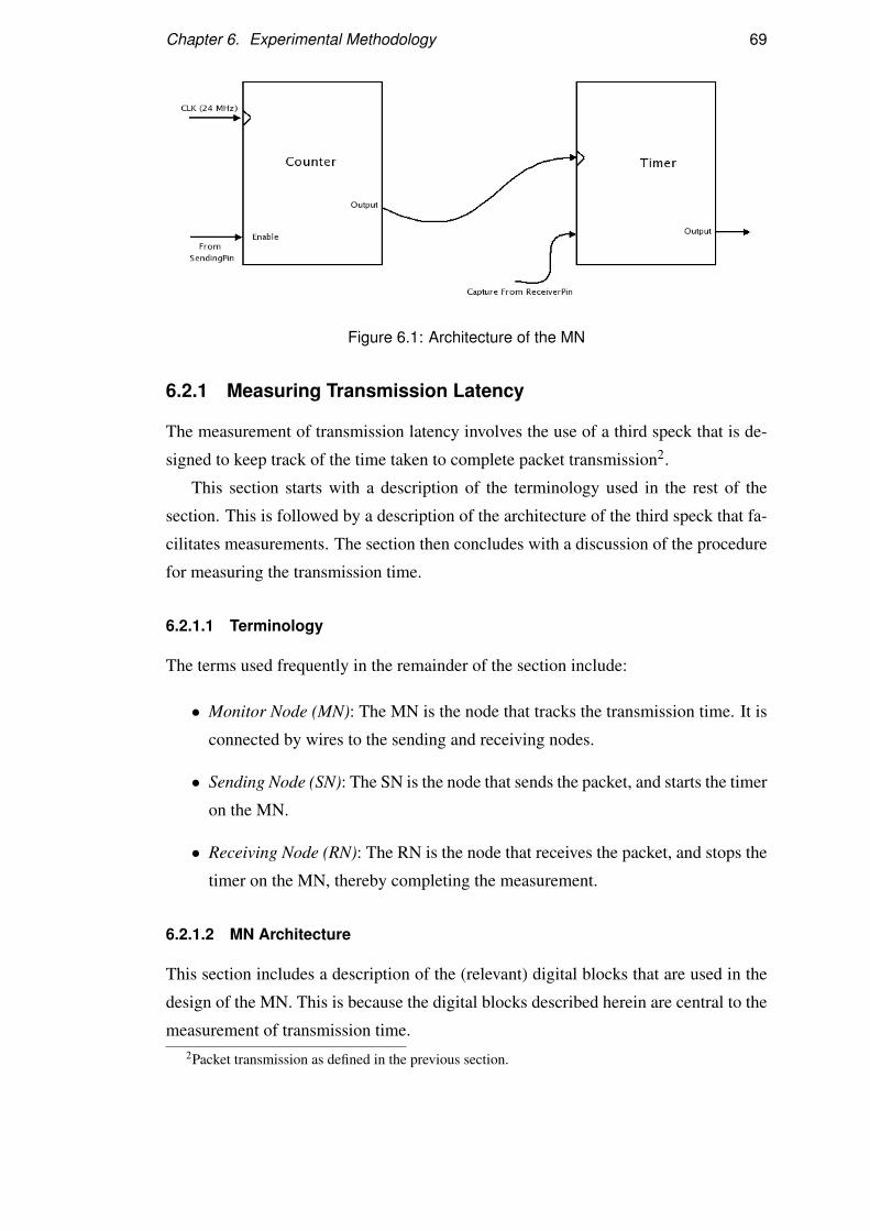
Chapter 6. Experimental Methodology 69
Figure 6.1: Architecture of the MN
6.2.1 Measuring Transmission Latency
The measurement of transmission latency involves the use of a third speck that is de-
signed to keep track of the time taken to complete packet transmission2.
This section starts with a description of the terminology used in the rest of the
section. This is followed by a description of the architecture of the third speck that fa-
cilitates measurements. The section then concludes with a discussion of the procedure
for measuring the transmission time.
6.2.1.1 Terminology
The terms used frequently in the remainder of the section include:
• Monitor Node (MN): The MN is the node that tracks the transmission time. It is
connected by wires to the sending and receiving nodes.
• Sending Node (SN): The SN is the node that sends the packet, and starts the timer
on the MN.
• Receiving Node (RN): The RN is the node that receives the packet, and stops the
timer on the MN, thereby completing the measurement.
6.2.1.2 MN Architecture
This section includes a description of the (relevant) digital blocks that are used in the
design of the MN. This is because the digital blocks described herein are central to the
measurement of transmission time.2Packet transmission as defined in the previous section.
Chapter 6. Experimental Methodology 70
The circuit consists of an 16 bit Timer (13) and an 8 bit Counter (11) that clocks
the timer; i.e., the output of the Counter is connected to the input of the Timer. This is
shown in Figure 6.1.
The Counter’s Enable input is connected to a pin at the SN. When the SN begins
to assemble the packet, it sets the pin, called the SenderPin, high. The Counter is then
enabled, and begins to clock the Timer.
When the packet is received at the final destination, the network layer entity at the
RN sets a pin, called the ReceiverPin, high. This is connected to the Capture input of
the Timer, which is set to interrupt on Capture.
When a Timer is set to interrupt on Capture, the countdown timer stops and the
value of the Compare register can be read out. Then, the time elapsed may be calcu-
lated using the following equation:
TimeElapsed = SourceClockPeriod×(PeriodRegisterValue−CompareRegisterValue)
(6.1)
where the PeriodRegisterValue is loaded with the maximum value possible for the
Timer type.
The result of 6.1 is then communicated to the PC using a UART (14).
6.2.1.3 Measurement Procedure for the DSDV algorithm
The procedure for transmission time measurement is a multi-step process as shown in
Figure 6.2. The stages are summarised below:
1. The SenderPin and the ReceiverPin of the SN and RN respectively are connected
to the appropriate pins on the MN (which are wired to the Enable input of the
Counter and the Capture input of the timer respectively).
2. The SN, upon identifying the RN, attempts to discover the route to the RN.
3. The SN set the SenderPin high, which enables the Counter and starts the Timer
on the MN.
4. Upon completion of the discovery of the route to the RN, the SN assembles the
Data packet to be sent to the RN.
5. The SN sends the Data packet using the MAC Layer primitives described in
Section 3.2.1.1.
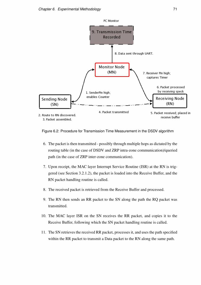
Chapter 6. Experimental Methodology 71
Figure 6.2: Procedure for Transmission Time Measurement in the DSDV algorithm
6. The packet is then transmitted - possibly through multiple hops as dictated by the
routing table (in the case of DSDV and ZRP intra-zone communication)/queried
path (in the case of ZRP inter-zone communication).
7. Upon receipt, the MAC layer Interrupt Service Routine (ISR) at the RN is trig-
gered (see Section 3.2.1.2), the packet is loaded into the Receive Buffer, and the
RN packet handling routine is called.
8. The received packet is retrieved from the Receive Buffer and processed.
9. The RN then sends an RR packet to the SN along the path the RQ packet was
transmitted.
10. The MAC layer ISR on the SN receives the RR packet, and copies it to the
Receive Buffer, following which the SN packet handling routine is called.
11. The SN retrieves the received RR packet, processes it, and uses the path specified
within the RR packet to transmit a Data packet to the RN along the same path.
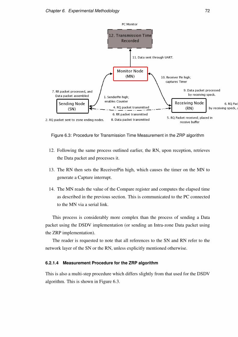
Chapter 6. Experimental Methodology 72
Figure 6.3: Procedure for Transmission Time Measurement in the ZRP algorithm
12. Following the same process outlined earlier, the RN, upon reception, retrieves
the Data packet and processes it.
13. The RN then sets the ReceiverPin high, which causes the timer on the MN to
generate a Capture interrupt.
14. The MN reads the value of the Compare register and computes the elapsed time
as described in the previous section. This is communicated to the PC connected
to the MN via a serial link.
This process is considerably more complex than the process of sending a Data
packet using the DSDV implementation (or sending an Intra-zone Data packet using
the ZRP implementation).
The reader is requested to note that all references to the SN and RN refer to the
network layer of the SN or the RN, unless explicitly mentioned otherwise.
6.2.1.4 Measurement Procedure for the ZRP algorithm
This is also a multi-step procedure which differs slightly from that used for the DSDV
algorithm. This is shown in Figure 6.3.
Chapter 6. Experimental Methodology 73
Instead of sending a Data packet, the SN sends an RQ packet (RQ packets are
central to reactive inter-zone communication described in Section 5.4).
This RQ packet is transmitted along the network until it reaches the first node that
has the RN within its routing zone. This node asserts the ReceiverPin which triggers
the Capture input on the MN.
The rest of the procedure is as described previously.
6.2.2 Measuring Delivery Ratio
The method used for measurement of Delivery Ratio is simpler than that used for
calculating the transmission time. However, the approach taken for calculating the
Delivery Ratio for the DSDV and ZRP algorithms varies slightly.
6.2.2.1 Technique used in DSDV characterisation
The two types of Data packets in the DSDV algorithm are Data packets and Acknowl-
edgement packets (see Section 3.2.2 for details). The measurement methodology uses
both packet types to measure the Delivery Ratio as follows:
• The SN sends Data packets at regular intervals to the RN which may be several
hops away.
• When the RN receives a Data packet, it increments a counter.
• When the sequence number of a received Data packet equals or exceeds a user-
defined threshold, the RN sends an Acknowledgement packet containing the
number of received packets in the payload.
• Upon receipt of the Acknowledgement packet, the SN calculates the Delivery
Ratio.
• Additionally, the SN resets its sequence number counter
The Delivery Ratio is calculated at the SN using the following equation:
Rdel =PktRx
PktT x×100 (6.2)
where:
Rdel is the Delivery Ratio (percentage),
PktRx is the number of packets received at the RN, and
PktT x is the number of packets sent at the SN.
Chapter 6. Experimental Methodology 74
6.2.2.2 Technique used in ZRP characterisation
The ZRP algorithm uses RQ and RR packets to calculate the delivery ratio, as op-
posed to the Data and Acknowledgement packets used in the analysis of the DSDV
implementation. The procedure involved may be described as follows:
• The SN sends an RQ packet to query a path to the RN, which is not in the same
zone as the SN.
• Upon receipt of an RQ packet, a zone-ending node in the same zone as the RN
sends an RR packet to the SN.
• The SN keeps count of the number of RQ packets sent and the number of
RR packets received. When the number of RQ packets exceeds a user-defined
threshold, the SN calculates the delivery ratio and communicates it to the PC
using a UART (14).
The delivery ratio of the ZRP implementation is also calculated using Equation 6.2.
6.2.3 Measuring Tx/Rx On-time
The On-time for the transmitter and the receiver are two distinct metrics measured
during the operation of the algorithm/application being evaluated.
The procedure for measuring Transmitter/Receiver On-time is by starting and stop-
ping timers when the transmitter or receiver of the CC2420 radio used on the Prospeckz
IIK (4) is turned on or off.
This section first presents the operation of the Timer digital block (13) available
on the PSoC CY8C29666 (12), followed by a brief description of the terminology and
procedure used for measuring Tx/Rx On-time used in this work.
6.2.3.1 Timer Operation
The timers available on the PSoC (13) operate as down counters, with the Count regis-
ter being loaded with the value in the Period register, and then being decremented with
each rising edge of the clock.
Therefore, the time elapsed between starting a timer and subsequently stopping it
may be calculated from the following equation:
TimeElapsed = (SourceClockPeriod)× (Countold −Countnew) (6.3)

Chapter 6. Experimental Methodology 75
where:
Countold is the value of the Count register when the timer started running, and
Countnew is the value of the Count register when the timer is stopped.
6.2.3.2 Terminology
• Global Counter (GC): This counter variable keeps track of the total time elapsed.
When the value of the counter reaches a user-defined threshold, the values of the
other two counters described below are read out and reset.
• Transmit Counter (TC): This counter variable holds the total time for which the
transmitter is turned on. The TC is periodically reset as described above.
• Receive Counter (RC): This counter variable holds the total time for which the
receiver is turned on. The RC, like the TC, is also periodically reset.
6.2.3.3 Technique used for measuring Tx/Rx On-time
As described above, a timer is turned on whenever the transmitter or receiver is turned
on. When it is turned back off, the timer is stopped.
The time elapsed during this interval is calculated using equation 6.3, and added to
the appropriate counter (TC or RC).
When the value of GC crosses a user-defined threshold3, the values of TC and RC
are read out, and the Tx/Rx On-time is calculated using the following equations:
T x Ontime =TCGC
(6.4)
Rx Ontime =TCGC
(6.5)
where all of the terms in the equation have the meanings defined earlier.
This is output to the PC via a serial link using a UART (14).
6.2.4 Measuring Metrics for Application Characterisation
This section details the techniques used to measure the values of metrics introduced in
Section 6.1.4 that are used only for the characterisation of the application.
3This threshold is set to 60 seconds during the course of the analyses performed as part of this work
Chapter 6. Experimental Methodology 76
6.2.4.1 Current and Power Consumption
This metric is measured by connecting a node running the application in series with an
ammeter (34). The value read by the ammeter is sampled periodically4, and transmitted
to the PC via a serial link.
The power consumed is calculated using the relationship between current, voltage
and power defined in the following equation:
P = V × I (6.6)
where:
P is the power consumed,
V is the voltage consumed, and
I is the current consumed.
6.2.4.2 CPU On-time
The CPU On-time is measured by starting and stopping a timer every time the CPU is
switched into and out of sleep mode respectively. This happens whenever an attempted
transmission has to wait because the transmission medium is busy.
The timer operates as described in Section 6.2.3.1. Also, the experimental setup is
similar to that used for measuring Tx/Rx On-time, as the counter variable GC is used
to keep track of the total elapsed time. A counter variable, CPU Counter (CC) keeps
track of the cumulative CPU On-time.
Whenever the value of GC crosses the user-defined threshold, it reads the value of
CC, and calculates the CPU On-time using the following equation:
CPU Ontime =CCGC
(6.7)
where all of the terms in the equation have the meanings defined earlier.
The value of CC is then reset, and the calculated CPU On-time is transmitted to the
PC using a UART.
6.3 Summary
This chapter described the metrics used for characterisation of the algorithms and ap-
plications implemented as part of this work. This was followed by a detailed descrip-4The sampling rate for the experiments run was 1 Hz.

Chapter 6. Experimental Methodology 77
tion of the techniques used to perform measurements on these metrics, as well as the
differences between the different implementations while performing the analyses of
the same metric.
Chapter 7
Characterisation and Analysis of the
DSDV Algorithm
This chapter presents the results obtained upon the characterisation of the DSDV algo-
rithm and analysis of the results thus obtained.
This chapter is organised as follows. The first section presents the results obtained
upon analysing the transmission time of the DSDV algorithm. The section that follows
discusses the results obtained upon analysis of the delivery ratio of the algorithm, while
the final section presents the results obtained upon running experiments on the Tx/Rx
On-time for the DSDV algorithm.
All of the experiments were performed using the methodology described in Chapter
6 on the algorithm presented in Chapter 3.
7.1 Transmission Time
The transmission time of the DSDV algorithm was measured using the setup described
in Section 6.2.1. Two Prospeckz IIK (4) nodes running the DSDV implementation
were connected by means of wires to a third Prospeckz IIK node running the MN
application.
The network topology was arranged so that a third node was required to facilitate
communication between the two nodes connected to the MN.
When the ReceiverPin at the MN is raised high, the MN resets the SenderPin and
the ReceiverPin. Upon this, the SN clears its routing table information. This is because
the transmission time measured for the DSDV algorithm includes the route discovery
time.
78
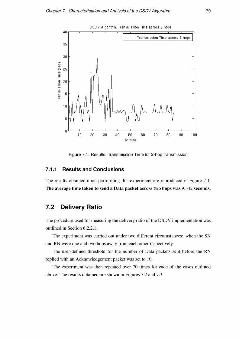
Chapter 7. Characterisation and Analysis of the DSDV Algorithm 79
Figure 7.1: Results: Transmission Time for 2-hop transmission
7.1.1 Results and Conclusions
The results obtained upon performing this experiment are reproduced in Figure 7.1.
The average time taken to send a Data packet across two hops was 9.342 seconds.
7.2 Delivery Ratio
The procedure used for measuring the delivery ratio of the DSDV implementation was
outlined in Section 6.2.2.1.
The experiment was carried out under two different circumstances: when the SN
and RN were one and two hops away from each other respectively.
The user-defined threshold for the number of Data packets sent before the RN
replied with an Acknowledgement packet was set to 10.
The experiment was then repeated over 70 times for each of the cases outlined
above. The results obtained are shown in Figures 7.2 and 7.3.
Chapter 7. Characterisation and Analysis of the DSDV Algorithm 80
7.2.1 Results
The delivery ratio for 1 hop transmission (the SN and RN are direct neighbours) was
found to be 99.85%, which was the delivery ratio obtained upon characterisations per-
formed on the SpeckMAC algorithm. Across 2 hops, the delivery ratio was found to
drop to 98.87%, which is lower than what one would anticipate considering the drop
across 1 hop. Battery failure - which may be classified as experimental error - during
the course of the experiment is responsible for the dips in the value of the delivery
ratio.
7.2.2 Conclusions
The following conclusions may be derived from the results obtained herein:
1. The DSDV algorithm is sufficiently robust as delivery ratio remains significantly
high across multiple hops.
2. The drop in the delivery ratio cannot be attributed to the MAC Layer delivery
ratio alone, but to interference between large numbers of packets from different
sources.
7.3 Tx/Rx On-time
The Tx/Rx On-time is measured using the procedure described in Section 6.2.3. The
Tx/Rx On-time for the DSDV algorithm was measured for a node with 7 neighbours,
where 7 was the maximum size the routing table was limited to.
7.3.1 Results
The results obtained are shown in Figure 7.4. The average proportion of time the
transmitter remained switched on was found to be an extremely small 1.1 seconds per
minute, which corresponds to 1.83% of the time. The receiver remains, on average,
switched on for a slightly larger proportion of time; approximately 1.6 seconds per
minute, which corresponds to 2.67% of the time.
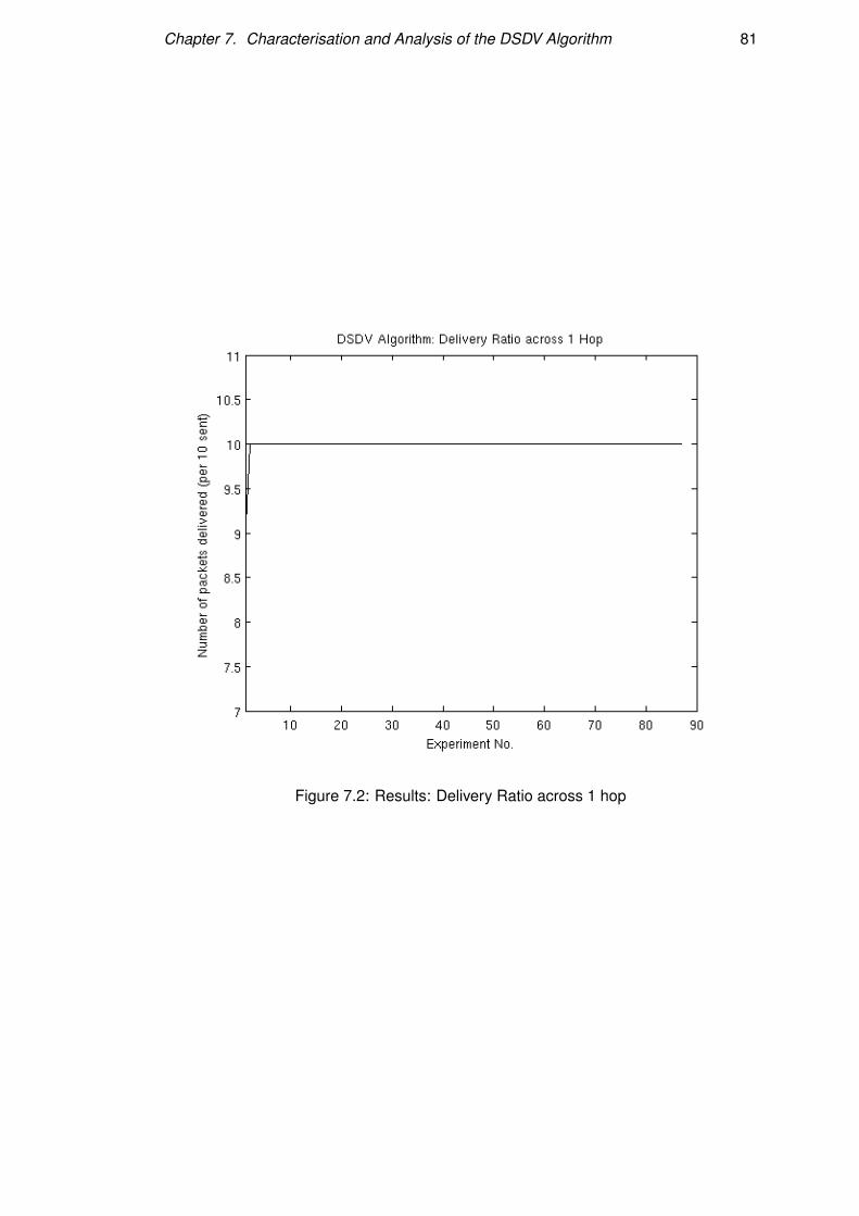
Chapter 7. Characterisation and Analysis of the DSDV Algorithm 81
Figure 7.2: Results: Delivery Ratio across 1 hop
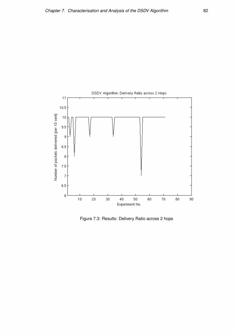
Chapter 7. Characterisation and Analysis of the DSDV Algorithm 82
Figure 7.3: Results: Delivery Ratio across 2 hops
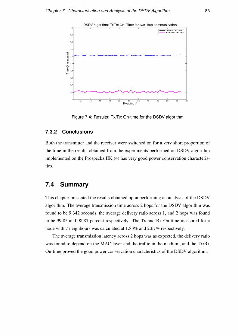
Chapter 7. Characterisation and Analysis of the DSDV Algorithm 83
Figure 7.4: Results: Tx/Rx On-time for the DSDV algorithm
7.3.2 Conclusions
Both the transmitter and the receiver were switched on for a very short proportion of
the time in the results obtained from the experiments performed on DSDV algorithm
implemented on the Prospeckz IIK (4) has very good power conservation characteris-
tics.
7.4 Summary
This chapter presented the results obtained upon performing an analysis of the DSDV
algorithm. The average transmission time across 2 hops for the DSDV algorithm was
found to be 9.342 seconds, the average delivery ratio across 1, and 2 hops was found
to be 99.85 and 98.87 percent respectively. The Tx and Rx On-time measured for a
node with 7 neighbours was calculated at 1.83% and 2.67% respectively.
The average transmission latency across 2 hops was as expected, the delivery ratio
was found to depend on the MAC layer and the traffic in the medium, and the Tx/Rx
On-time proved the good power conservation characteristics of the DSDV algorithm.
Chapter 8
Characterisation and Analysis of the
VTS Application
This chapter contains details of the experiments performed to characterise the VTS
application (see Chapter 4), and the analysis of the results obtained.
The metrics used for the analysis of the VTS application are different from those
used to perform the analysis of the DSDV algorithm for reasons outlined in Section
6.1.4. Additionally, the Tx/Rx On-time was also measured.
The experiments performed on the application attempted to analyse the feasibility
and potential cost of deploying the application.
This chapter begins with a short rationale on the differing requirements for the
different node types used in the VTS. This is followed by a short description of the
experimental setup used during the performance of the experiments on the VTS. The
next three sections provide the reader with the results obtained upon measuring the
Tx/Rx On-time, the CPU On-time, and Current/Power consumption, and discusses the
inferences derived from the results.
8.1 Varying Requirements for different VTS node types:
The Rationale
The VTS has three types of nodes: INs fixed to the walls, the MN carried by the
monitoring agent, and the VNs affixed to visitors to the built-in environment.
Each of the three has different requirements, as a result of which their architectures
differ.
84
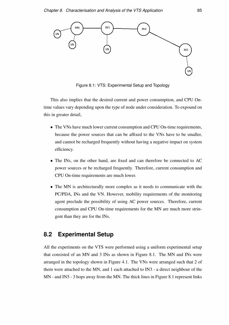
Chapter 8. Characterisation and Analysis of the VTS Application 85
Figure 8.1: VTS: Experimental Setup and Topology
This also implies that the desired current and power consumption, and CPU On-
time values vary depending upon the type of node under consideration. To expound on
this in greater detail,
• The VNs have much lower current consumption and CPU On-time requirements,
because the power sources that can be affixed to the VNs have to be smaller,
and cannot be recharged frequently without having a negative impact on system
efficiency.
• The INs, on the other hand, are fixed and can therefore be connected to AC
power sources or be recharged frequently. Therefore, current consumption and
CPU On-time requirements are much lower.
• The MN is architecturally more complex as it needs to communicate with the
PC/PDA, INs and the VN. However, mobility requirements of the monitoring
agent preclude the possibility of using AC power sources. Therefore, current
consumption and CPU On-time requirements for the MN are much more strin-
gent than they are for the INs.
8.2 Experimental Setup
All the experiments on the VTS were performed using a uniform experimental setup
that consisted of an MN and 3 INs as shown in Figure 8.1. The MN and INs were
arranged in the topology shown in Figure 4.1. The VNs were arranged such that 2 of
them were attached to the MN, and 1 each attached to IN3 - a direct neighbour of the
MN - and IN5 - 3 hops away from the MN. The thick lines in Figure 8.1 represent links
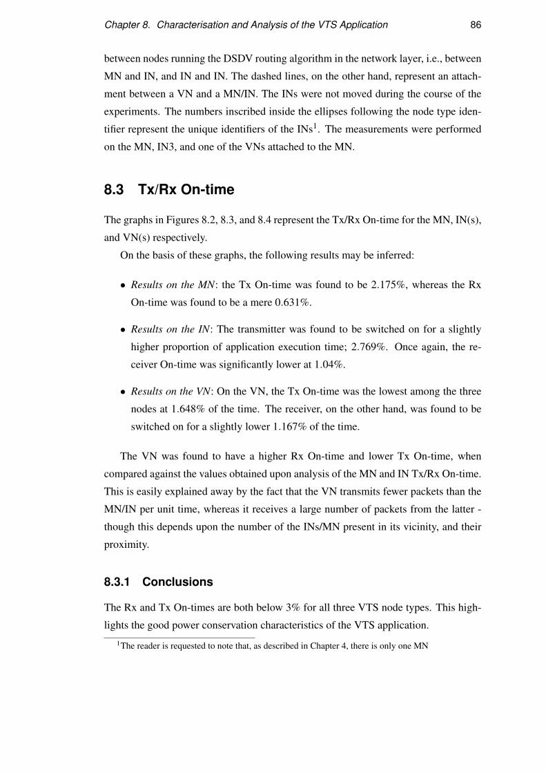
Chapter 8. Characterisation and Analysis of the VTS Application 86
between nodes running the DSDV routing algorithm in the network layer, i.e., between
MN and IN, and IN and IN. The dashed lines, on the other hand, represent an attach-
ment between a VN and a MN/IN. The INs were not moved during the course of the
experiments. The numbers inscribed inside the ellipses following the node type iden-
tifier represent the unique identifiers of the INs1. The measurements were performed
on the MN, IN3, and one of the VNs attached to the MN.
8.3 Tx/Rx On-time
The graphs in Figures 8.2, 8.3, and 8.4 represent the Tx/Rx On-time for the MN, IN(s),
and VN(s) respectively.
On the basis of these graphs, the following results may be inferred:
• Results on the MN: the Tx On-time was found to be 2.175%, whereas the Rx
On-time was found to be a mere 0.631%.
• Results on the IN: The transmitter was found to be switched on for a slightly
higher proportion of application execution time; 2.769%. Once again, the re-
ceiver On-time was significantly lower at 1.04%.
• Results on the VN: On the VN, the Tx On-time was the lowest among the three
nodes at 1.648% of the time. The receiver, on the other hand, was found to be
switched on for a slightly lower 1.167% of the time.
The VN was found to have a higher Rx On-time and lower Tx On-time, when
compared against the values obtained upon analysis of the MN and IN Tx/Rx On-time.
This is easily explained away by the fact that the VN transmits fewer packets than the
MN/IN per unit time, whereas it receives a large number of packets from the latter -
though this depends upon the number of the INs/MN present in its vicinity, and their
proximity.
8.3.1 Conclusions
The Rx and Tx On-times are both below 3% for all three VTS node types. This high-
lights the good power conservation characteristics of the VTS application.
1The reader is requested to note that, as described in Chapter 4, there is only one MN
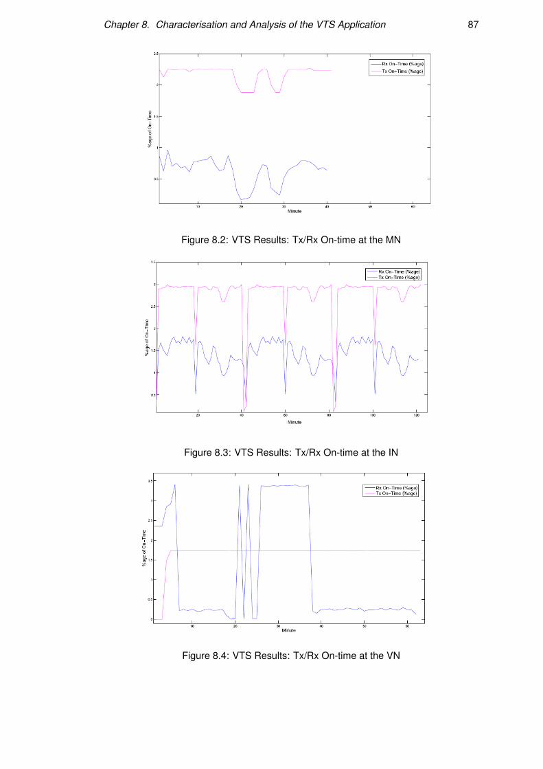
Chapter 8. Characterisation and Analysis of the VTS Application 87
Figure 8.2: VTS Results: Tx/Rx On-time at the MN
Figure 8.3: VTS Results: Tx/Rx On-time at the IN
Figure 8.4: VTS Results: Tx/Rx On-time at the VN
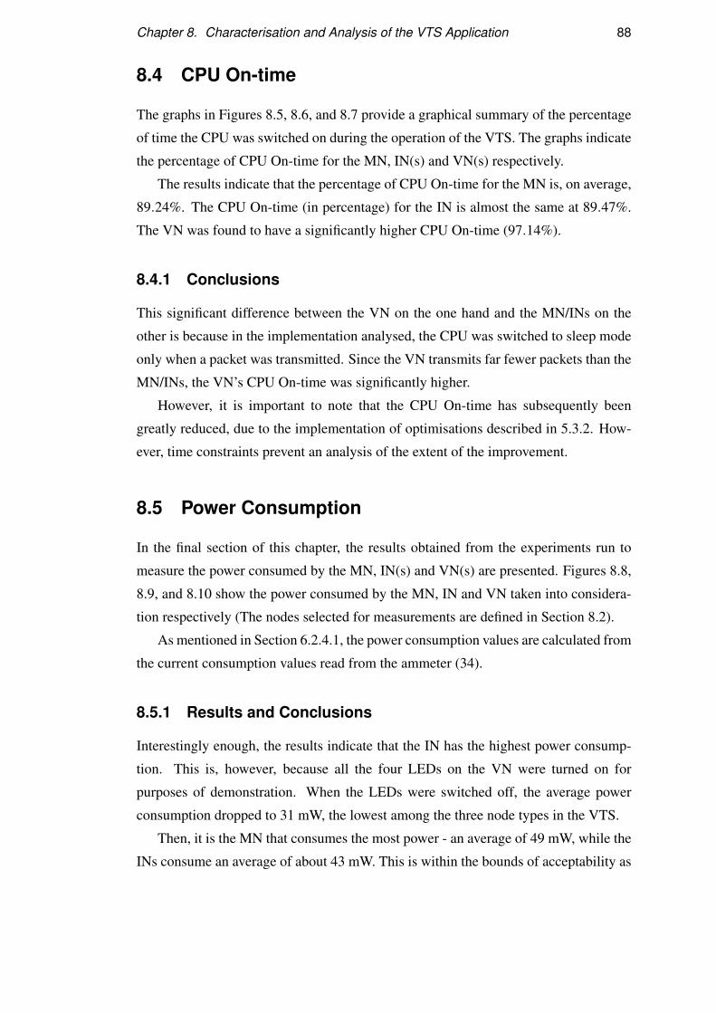
Chapter 8. Characterisation and Analysis of the VTS Application 88
8.4 CPU On-time
The graphs in Figures 8.5, 8.6, and 8.7 provide a graphical summary of the percentage
of time the CPU was switched on during the operation of the VTS. The graphs indicate
the percentage of CPU On-time for the MN, IN(s) and VN(s) respectively.
The results indicate that the percentage of CPU On-time for the MN is, on average,
89.24%. The CPU On-time (in percentage) for the IN is almost the same at 89.47%.
The VN was found to have a significantly higher CPU On-time (97.14%).
8.4.1 Conclusions
This significant difference between the VN on the one hand and the MN/INs on the
other is because in the implementation analysed, the CPU was switched to sleep mode
only when a packet was transmitted. Since the VN transmits far fewer packets than the
MN/INs, the VN’s CPU On-time was significantly higher.
However, it is important to note that the CPU On-time has subsequently been
greatly reduced, due to the implementation of optimisations described in 5.3.2. How-
ever, time constraints prevent an analysis of the extent of the improvement.
8.5 Power Consumption
In the final section of this chapter, the results obtained from the experiments run to
measure the power consumed by the MN, IN(s) and VN(s) are presented. Figures 8.8,
8.9, and 8.10 show the power consumed by the MN, IN and VN taken into considera-
tion respectively (The nodes selected for measurements are defined in Section 8.2).
As mentioned in Section 6.2.4.1, the power consumption values are calculated from
the current consumption values read from the ammeter (34).
8.5.1 Results and Conclusions
Interestingly enough, the results indicate that the IN has the highest power consump-
tion. This is, however, because all the four LEDs on the VN were turned on for
purposes of demonstration. When the LEDs were switched off, the average power
consumption dropped to 31 mW, the lowest among the three node types in the VTS.
Then, it is the MN that consumes the most power - an average of 49 mW, while the
INs consume an average of about 43 mW. This is within the bounds of acceptability as
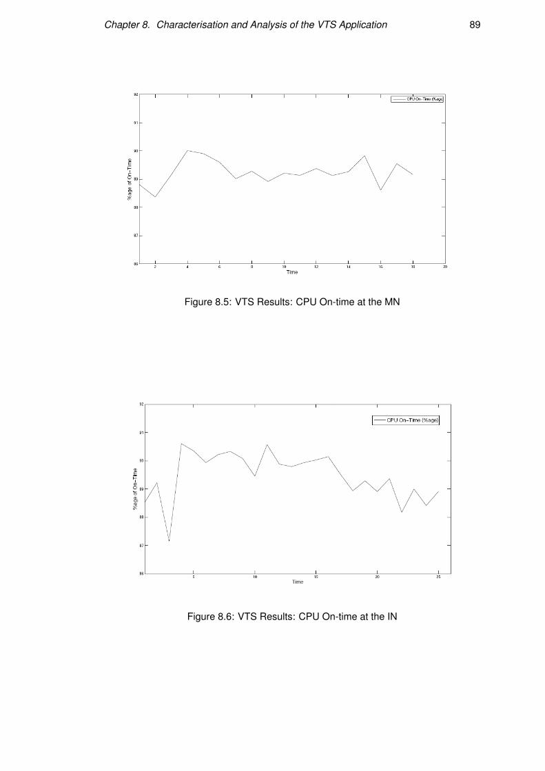
Chapter 8. Characterisation and Analysis of the VTS Application 89
Figure 8.5: VTS Results: CPU On-time at the MN
Figure 8.6: VTS Results: CPU On-time at the IN
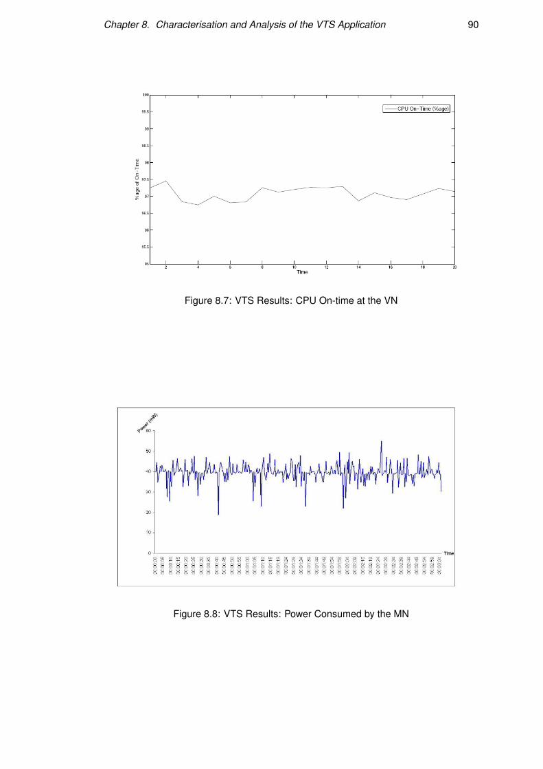
Chapter 8. Characterisation and Analysis of the VTS Application 90
Figure 8.7: VTS Results: CPU On-time at the VN
Figure 8.8: VTS Results: Power Consumed by the MN
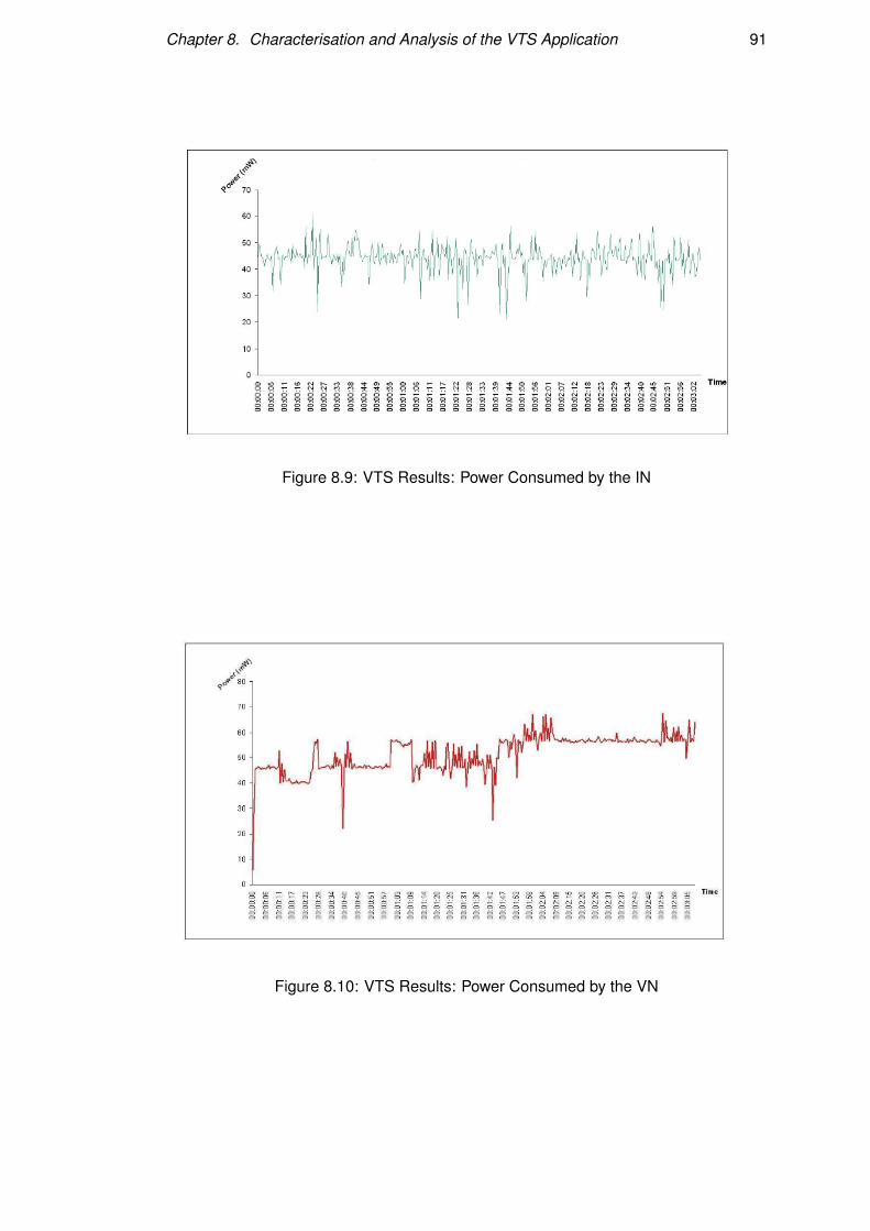
Chapter 8. Characterisation and Analysis of the VTS Application 91
Figure 8.9: VTS Results: Power Consumed by the IN
Figure 8.10: VTS Results: Power Consumed by the VN
Chapter 8. Characterisation and Analysis of the VTS Application 92
the MN has the most complex architecture of the three, and communicates both with
the INs and VNs (using RF communication), as well as the PC/PDA (using a serial
link).
Chapter 9
Characterisation and Analysis of the
ZRP Algorithm
This chapter presents the results obtained upon the characterisation of the ZRP algo-
rithm and analysis of the results thus obtained.
This chapter is organised as follows. The first section presents the results obtained
upon analysing the transmission time of the ZRP algorithm. The section that follows
discusses the results obtained upon analysis of the delivery ratio of the algorithm, while
the final section presents the results obtained upon running experiments on the Tx/Rx
On-time for the ZRP algorithm.
All of the experiments were performed using the methodology described in Chapter
6 on the algorithm presented in Chapter 5.
As mentioned in Chapter 6, the results obtained from the analysis of the ZRP and
DSDV algorithms are comparable in spite of the changes made to the DSDV imple-
mentation in the course of the implementation of the ZRP algorithm. This is because
the experiments on the DSDV algorithm were re-run on the modified (and improved)
implementation to facilitate comparison.
Note: All of the experiments on the ZRP algorithm were carried out with the zone
radius set to 1, and the inter-zone route caching mechanism disabled.
9.1 Transmission Time
The analysis of the Transmission Time was performed using the methodology de-
scribed in Section 6.2.1. As described in Section 6.2.1.4, the methodology used in
the analysis of the transmission time measurement for the ZRP algorithm is longer.
93
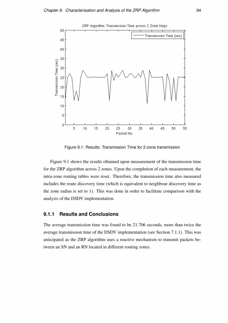
Chapter 9. Characterisation and Analysis of the ZRP Algorithm 94
Figure 9.1: Results: Transmission Time for 2-zone transmission
Figure 9.1 shows the results obtained upon measurement of the transmission time
for the ZRP algorithm across 2 zones. Upon the completion of each measurement, the
intra-zone routing tables were reset. Therefore, the transmission time also measured
includes the route discovery time (which is equivalent to neighbour discovery time as
the zone radius is set to 1). This was done in order to facilitate comparison with the
analysis of the DSDV implementation.
9.1.1 Results and Conclusions
The average transmission time was found to be 21.706 seconds, more than twice the
average transmission time of the DSDV implementation (see Section 7.1.1). This was
anticipated as the ZRP algorithm uses a reactive mechanism to transmit packets be-
tween an SN and an RN located in different routing zones.
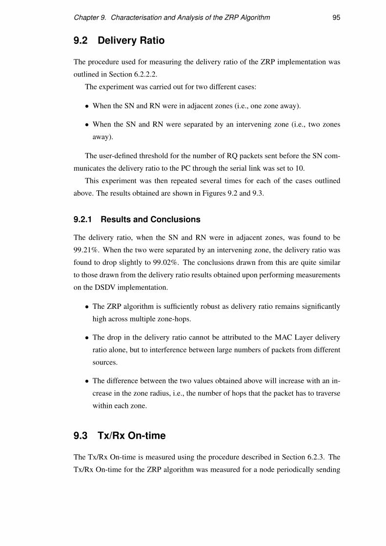
Chapter 9. Characterisation and Analysis of the ZRP Algorithm 95
9.2 Delivery Ratio
The procedure used for measuring the delivery ratio of the ZRP implementation was
outlined in Section 6.2.2.2.
The experiment was carried out for two different cases:
• When the SN and RN were in adjacent zones (i.e., one zone away).
• When the SN and RN were separated by an intervening zone (i.e., two zones
away).
The user-defined threshold for the number of RQ packets sent before the SN com-
municates the delivery ratio to the PC through the serial link was set to 10.
This experiment was then repeated several times for each of the cases outlined
above. The results obtained are shown in Figures 9.2 and 9.3.
9.2.1 Results and Conclusions
The delivery ratio, when the SN and RN were in adjacent zones, was found to be
99.21%. When the two were separated by an intervening zone, the delivery ratio was
found to drop slightly to 99.02%. The conclusions drawn from this are quite similar
to those drawn from the delivery ratio results obtained upon performing measurements
on the DSDV implementation.
• The ZRP algorithm is sufficiently robust as delivery ratio remains significantly
high across multiple zone-hops.
• The drop in the delivery ratio cannot be attributed to the MAC Layer delivery
ratio alone, but to interference between large numbers of packets from different
sources.
• The difference between the two values obtained above will increase with an in-
crease in the zone radius, i.e., the number of hops that the packet has to traverse
within each zone.
9.3 Tx/Rx On-time
The Tx/Rx On-time is measured using the procedure described in Section 6.2.3. The
Tx/Rx On-time for the ZRP algorithm was measured for a node periodically sending
Chapter 9. Characterisation and Analysis of the ZRP Algorithm 96
Figure 9.2: Results: Delivery Ratio across 1 zone hop
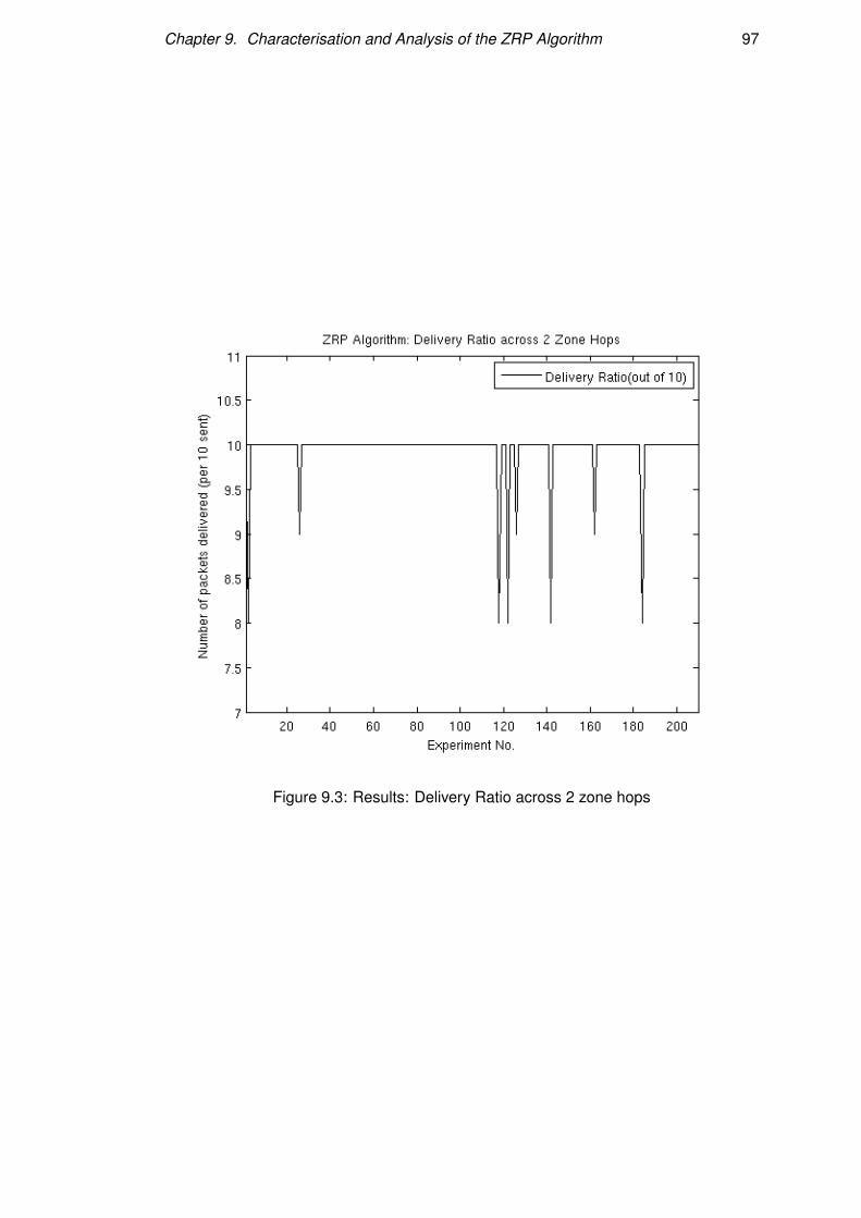
Chapter 9. Characterisation and Analysis of the ZRP Algorithm 97
Figure 9.3: Results: Delivery Ratio across 2 zone hops

Chapter 9. Characterisation and Analysis of the ZRP Algorithm 98
RQ packets to an RN two zones away. The experimental setup was thus the same as
that used for measuring transmission time.
The results obtained for Tx On-time are shown in Figure 9.4, and the results ob-
tained for Rx On-time are shown in Figure 9.5.
9.3.1 Results and Conclusions
The average proportion of time the transmitter remained switched on was found to
be 1.49 seconds per minute, which corresponds to 2.486% of the time. The receiver
remains, on average, switched on for only 64% of the time that the transmitter is turned
on; approximately 0.967 seconds per minute, which corresponds to a mere 1.612% of
the time.
9.3.1.1 Differences with DSDV Tx/Rx On-time Results
The measurements performed on the DSDV implementation indicated that the receiver
was turned on for a longer period of time than the transmitter. The converse is true in
the case of the measurements of Tx/Rx On-time for the ZRP implementation. This is
due to the following reasons:
• In the ZRP implementation, Tx/Rx On-time measurements were made of a node
that was periodically sending Data packets. This resulted in a high Tx On-time.
• The experimental setup, as well as the fragmentation of the network into smaller
zones resulted in a reduction in the number of neighbours that the node received
IRUs from. Therefore, the Rx On-time was correspondingly lower.
9.3.1.2 Dips in the Tx On-time graph
Figure 9.4 shows a number of dips in the Tx On-time. The use of the experimental
setup described in Section 9.1 resulted in the intra-zone routing table being erased
upon the completion of data transmission between the SN and RN. Therefore, in the
intervening period, the SN does not transmit Data packets as it is unaware of the nodes
at the boundary of its routing zone.
As a result of this, the transmitter is not turned on, and the recorded value of the
Tx On-time falls.

Chapter 9. Characterisation and Analysis of the ZRP Algorithm 99
Figure 9.4: Results: Tx On-time for the ZRP algorithm

Chapter 9. Characterisation and Analysis of the ZRP Algorithm 100
Figure 9.5: Results: Rx On-time for the ZRP algorithm
Chapter 9. Characterisation and Analysis of the ZRP Algorithm 101
9.4 Summary
This chapter presented the results obtained upon performing an analysis of the ZRP
algorithm. The average transmission time across 2 zones for the ZRP algorithm was
found to be more than twice the 2-hop transmission time for the DSDV implementation
at 21.706 seconds.
The average delivery ratio across 1, and 2 zone-hops was found to be extremely
high at 99.21 and 99.02 percent respectively - values comparable to those obtained
upon the analysis of the DSDV implementation.
The Tx and Rx On-time were measured to be 2.486% and 1.612% respectively.
The reasons behind the differences in the Tx/Rx On-time values obtained in the course
of the analysis of the ZRP and the DSDV implementations is explained in Section
9.3.1.1. Nonetheless, the Tx/Rx On-time values are extremely low, and are indicative
of the good power-conservation characteristics of the ZRP implementation presented
as part of this work.
Chapter 10
Comparison of ZRP and DSDV on
WSNs
Thus far, this work has presented the implementation and characterisation of both the
DSDV and ZRP algorithms. During the discussion of the characterisation of the latter,
references were made to perceivable differences in the results obtained upon charac-
terising the two algorithms.
This short chapter examines the implication of these differences. The chapter be-
gins with a short summary of the suitability of both algorithms on WSNs, and the next
section considers the relative merits and demerits of each algorithm.
10.1 Suitability of the DSDV and ZRP algorithms
The open questions at the beginning of the thesis were whether MANET algorithms
such as the ZRP and DSDV algorithms could be used in failure-prone WSNs that
have more stringent energy and memory requirements, and if there were application
domains for WSNs suitable for the use of these algorithms.
Upon completion of the characterisation of both the algorithms in a real environ-
ment, the following conclusions were arrived upon:
• Both algorithms fit into the limited memory available on the ProSpeckz IIK (4).
• Both algorithms displayed good power conservation characteristics, as exempli-
fied by the proportions of time during which the transmitters and receivers on
the nodes running the algorithms were switched on.
102
Chapter 10. Comparison of ZRP and DSDV on WSNs 103
• The delivery ratio of packets was found in both cases to be greater than 98%
across 2 hops (or zone hops, in the case of the ZRP algorithm).
• Both algorithms were found to be fault-tolerant, as changes in network topology
due to node failure and movement were handled.
Additionally, in the course of this work, an application that used the DSDV al-
gorithm for communication was developed. The application, upon characterisation,
displayed good power conservation characteristics. This is because of both the duty
cycling in the MAC layer (38) as well as the design of the algorithms itself.
Possible applications for the ZRP algorithm have been considered and earmarked
for the future. These are discussed in the final chapter.
Thus, one can effectively conclude that the algorithms considered as part of this
work are suitable for use in WSNs, and that there exist application domains where
these algorithms can be put to efficient use.
10.2 DSDV vs ZRP
As discussed in the previous section, both the DSDV and ZRP algorithms displayed
good power conservation, fault tolerance, and data delivery characteristics. However,
the primary difference between the two algorithms becomes apparent upon considera-
tion of the transmission time.
The transmission time measured for the ZRP algorithm was more than twice the
transmission time for the DSDV algorithm. This is because the DSDV algorithm uses
a proactive scheme and is aware of every other node in the network. On the other hand,
the ZRP algorithm is a hybrid algorithm that uses a reactive scheme to determine routes
to nodes outside of the source node’s routing zone; thus, the ZRP algorithm maintains
routing information only for nodes within its zone.
Therfore, the DSDV algorithm is not as scalable as the ZRP algorithm is - espe-
cially given the memory constraints on sensor nodes. Many WSN applications require
routing between larger numbers of nodes than can be supported using the DSDV al-
gorithm. The ZRP algorithm, by virtue of its better scalability, can be used to enable
routing in these applications1. Some applications where the ZRP algorithm can be
used are discussed, as mentioned earlier, in the final chapter of this work.
1However, it is worth noting that the ZRP algorithm cannot be used efficiently for applications whichrequire thousands of possibly sparsely-connected nodes.
Chapter 11
Conclusions and Future Work
This work presented the implementation and characterisation of a selection of MANET
routing algorithms in WSNs. It additionally attempted to explore domains wherein
MANET routing algorithms could potentially be applied.
The dissertation began with a review of WSNs, and a detailed discussion of the
hardware and software platforms, MAC layer algorithms, and network layer algorithms
used (and developed) in this work.
This was followed by an in-depth presentation of the implementation of the DSDV
algorithm, an application that builds upon and uses the DSDV algorithm, and the ZRP
algorithm. This included descriptions of the position of the algorithm/application in
the protocol stack, the primitives used from the lower layers, and the data structures
and primitives defined as part of the algorithm/application.
The discussion then moved to the experimental methodology used to characterise
the implementations developed herein. The metrics used and the mechanisms used to
measure them were presented.
This report then detailed the results obtained upon performing the experiments,
and the conclusions derived from these results. The results indicated that the MANET
algorithms analysed herein were suitable for use in WSNs by virtue of their power
and memory conservation characteristics, and also that there exist application domains
where these algorithms may be used.
It is our belief that we have developed implementations on the ProSpeckz IIK (4)
that could be used in the future in developing novel applications, and that we have
performed a detailed analysis and comparison of two algorithms typically unused in
the WSN domain.
104
Chapter 11. Conclusions and Future Work 105
11.1 Future Work
This section provides an account of possible extensions to the work done as part of this
thesis. These include:
• Anti-flap mechanisms: To avoid stray radio signals from a node (“flapping”)
influencing the topology of the network and causing an increase in network ac-
tivity, an “anti-flap” mechanism can be developed. This mechanism could be
akin to the “route flap” damping (16) performed in the Border Gateway Protocol
(BGP) (17), wherein a route’s flapping is exponentially decayed.
• The analysis of the ZRP algorithm may be performed on a larger network, by
using the Perspeckz-64 (20) physical test-bed.
• The results obtained using the ProSpeckz IIK (4) may be reinforced by running
simulations of the algorithms.
• Additionally, the SpeckMAC (38) implementation in the MAC layer can be mod-
ified in order to prevent duplicates being read from the medium and placed in the
receive buffer.

Bibliography
[1] AKKAYA, K., AND YOUNIS, M. A Survey on Routing Protocols in Wireless
Sensor Networks. In Ad-hoc Networks (2005).
[2] AKYILDIZ, I. F., SU, W., SANKARASUBRMANIAN, Y., AND CAYIRCI, E. A
Survey on Sensor Networks. IEEE Communications Magazine (August 2002),
102–114.
[3] AL-KARAKI, J. N., AND KAMAL, A. E. Routing Techniques in Wireless Sensor
Networks: A Survey. IEEE Wireless Communications (December 2004), 6–28.
[4] ARVIND, D. K., AND WONG, K. J. Speckled Computing: Disruptive Technol-
ogy for Networked Information Appliances. In IEEE International Symposium
on Consumer Electronics (2004), pp. 219–223.
[5] AZUMA, R. Tracking requirements for augmented reality. Communications of
the ACM (1993), 50–51.
[6] BAHL, P., AND PADMANABHAN, V. RADAR: an in-building RF-based user
location and tracking system. In Proceedings of the Nineteenth Annual IEEE
Joint Conference of the IEEE Computer and Communications Societies (2000),
pp. 775–784.
[7] BAHL, P., PADMANABHAN, V., AND BALACHANDRAN, A. Enhancements to
the RADAR User Location and Tracking System. Microsoft Research Technical
Report MSR TR-2000-12, February 2000.
[8] BARNES, M., AND LING, M. The 5CubeOTS. 5th Workshop in Speckled Com-
puting, Edinburgh, September 2006.
[9] BELLMAN, R. On a Routing Problem. Quarterly of Applied Mathematics (1958),
87–90.
106
Bibliography 107
[10] CROW, B., WIDJAJA, I., KIM, L., AND SAKAI, P. IEEE 802.11 Wireless Local
Area Networks. IEEE Communications Magazine (1997), 116–126.
[11] CYPRESS MICROSYSTEMS. 8-, 16-, 24- and 32-bit Counters.
CY8C29/27/24/22xxx Data Sheet, 2003.
[12] CYPRESS MICROSYSTEMS. PSoC Mixed Signal Array Final Data Sheet for
CY8C29466, CY8C29566, CY8C29666, and CY8C29866, November 2003.
[13] CYPRESS MICROSYSTEMS. 8-, 16-, 24- and 32-bit Timers.
CY8C29/27/24/22/21xx and CYWUSB Data Sheet, October 2005.
[14] CYPRESS MICROSYSTEMS. UART v5.2. CY8C29/27/24/22/21xxx, CY7C64215,
and CYWUSB Data Sheet, October 2005.
[15] HAAS, Z. A new routing protocol for the reconfigurable wireless networks. In
Universal Personal Communications Record (1997).
[16] INTERNET ENGINEERING TASK FORCE. Request for Comments: 2439. BGP
Route Flap Damping, November.
[17] INTERNET ENGINEERING TASK FORCE. Request for Comments: 4271. A Bor-
der Gateway Protocol 4 (BGP-4), January 2006.
[18] J. CAFFERY, J., AND STUBER, G. Subscriber location in CDMA cellular net-
works. In IEEE Transactions on Vehicular Technology (1998), pp. 406–416.
[19] J.M. KAHN, R. K., AND PISTER, K. Next Century Challenges: Mobile
Networking for Smart Dust. In ACM MobiCom ’99, Washington, DC (1999),
pp. 271–278.
[20] KAI JUAN WONG, AND DAMAL K. ARVIND. Perspeckz-64: physical test-bed
for performance evaluation of MAC and networking algorithms for Specknets.
In Second international workshop on Multi-hop ad hoc networks: from theory to
reality (2006), pp. 122–124.
[21] KUROSE, J., AND ROSS, K. Computer Networking: A Top-Down Approach
featuring the Internet. Addison Wesley, 2004.
[22] MARK, B., AND ZAIDI, Z. Robust mobility tracking for cellular networks. In
IEEE International Conference on Communications (2002), pp. 445–449.
Bibliography 108
[23] MATTHEW BARNES, HUGH LEATHER, AND DAMAL K. ARVIND. Emergency
Evacuation using Wireless Sensor Networks (To be published). In 32nd IEEE
Conference on Local Computer Networks (October 2007).
[24] MOEGLEIN, M., AND KRASNER, N. An Introduction to SnapTrack Server-
Aided GPS Technology. In Proceedings of the International Technical Meeting
of the Satellite Division of the Institute of Navigation (ION GPS) (1998).
[25] NI, L. M., LIU, Y., LAU, Y. C., AND PATIL, A. P. LANDMARC: Indoor
Location Sensing using Active RFID. Wireless Networks (2004), 701–710.
[26] PERKINS, C. E., AND BHAGWAT, P. Highly Dynamic Destination-Sequenced
Distance-Vector Routing (DSDV) for Mobile Computers. ACM SIGCOMM
Computer Communication Review (October 1994), 234–244.
[27] POLASTRE, J., J.HILL, AND CULLER, D. Versatile low power media access for
wireless sensor networks. In Second ACM SenSys (2004).
[28] REARDON, C., CARISSON, C., AND KRAUSS, T. Specknet: Optical Network-
ing and Location Discovery. 5th Workshop in Speckled Computing, Edinburgh,
September 2006.
[29] SEGUINE, D. Just add sensor - integrating analog and digital signal conditioning
in a Programmable System on Chip. In IEEE Conference on Sensors (2002),
pp. 665–668.
[30] SMAILAGIC, A., AND KOGAN, D. Location sensing and privacy in a context-
aware computing environment. IEEE Wireless Communications (October 2002),
10–17.
[31] SRINIVASAN, K., AND LEVIS, P. RSSI is Under Appreciated. In Third ACM
Workshop on Embedded Network Devices (2006).
[32] TANNENBAUM, A. S. Computer Networks, 4th Edition, Second Indian
Reprint ed. Pearson Education (Singapore) Pte Ltd., Indian Branch, 1999.
[33] TEKINAY, S. Wireless Geolocation Systems and Services. IEEE Communica-
tions Magazine (1998), 28–28.
[34] TENMA TEST EQUIPMENT. Model 72-7755: Operating Manual.
Bibliography 109
[35] VAN DAM, T., AND LANGENDOEN, K. An Adaptive Energy-Efficient MAC
Protocol for Wireless Sensor Networks. In ACM SenSys (2003), pp. 171–180.
[36] WANT, R., HOPPER, A., FALCAO, V., AND GIBBONS, J. The active badge
location system. ACM Transactions on Information Systems (1992), 91–102.
[37] WEISER, M. Hot Topics - Ubiquitous Computing. IEEE Computer (October
1993), 71–72.
[38] WONG, K. J., AND ARVIND, D. K. SpeckMAC: low-power decentralised MAC
protocols for low data rate transmissions in Specknets. In Second International
Workshop on Multi-hop ad-hoc networks (2006), pp. 71–78.
[39] YE, W., HEIDEMANN, J., AND ESTRIN, D. An energy-efficient MAC protocol
for wireless sensor networks. In 21st Conference of the IEEE Computer and
Communication Societies (2002), vol. 3.


![EXPERIMENTAL EVALUATION OF LSPR ROUTING PROTOCOL€¦ · Demand-driven Routing Protocol for MANET[] AODV is a packet routing protocol designed for use in mobile ad hoc networks (MANET)](https://img.pdfslide.us/doc/110x75/5f526102bcd353229e7c4523/experimental-evaluation-of-lspr-routing-protocol-demand-driven-routing-protocol.jpg)


![Zone Based Ant Colony Routing in MANET[Report]](https://img.pdfslide.us/doc/110x75/5534d5f84a7959dc528b4cca/zone-based-ant-colony-routing-in-manetreport.jpg)