Embed Size (px)
Citation preview

Algorithmic Techniques in VLSI CAD
Shantanu Dutt
University of Illinois at Chicago

Common Algorithmic Approaches in VLSI CAD
• Divide & Conquer (D&C) [e.g., merge-sort, partition-driven placement, tech.mapping of fanout-free ckt for dynamic power min.]
• Reduce & Conquer (R&C) [e.g., multilevel techniques such as the hMetis partitioner]
• Dynamic programming [e.g., matrix multiplication, optimal buffer insertion]
• Mathematical programming: linear, quadratic, 0/1 integer programming [e.g., floorplanning, global placement]

Common Algorithmic Approaches in VLSI CAD (contd)
• Search Methods:– Depth-first search (DFS): mainly used to find any
solution when cost is not an issue [e.g., FPGA detailed routing---cost generally determined at the global routing phase]
– Breadth-first search (BFS): mainly used to find a soln at min. distance from root of search tree [e.g., maze routing when cost = dist. from root]
– Best-first search (BeFS): used to find optimal or provably sub-optimal (at most a certain given factor of optimal) solutions w/ any cost function, Can be done when a provable lower-bound of the cost can be determined for each branching choice from the “current partial soln node” [e.g., TSP, global routing]
• Iterative Improvement: deterministic, stochastic• Min-cost network flow

Divide & Conquer• Determine if the problem can be solved in a hierarchical or divide-&-
conquer (D&C) manner:
– D&C approach: See if the problem can be “broken up” into 2 or more smaller subproblems that can be “stitched-up” to give a soln. to the parent prob.– Do this recrusively for each large subprob until subprobs are small enough for an “easy” solution technique (could be exhasutive!)– If the subprobs are of a similar kind to the root prob then the breakup and stitching will also be similar–The final design may or may not be optimal (will be optimal if the problem has the dynamic programming property; see later)
Subprob. A1
A1,1 A1,2 A2,1 A2,2
Root problem A
Subprob. A2
Stitch-up of solns to A1 and A2to form the complete soln to A
Do recursively until subprob-size is s.t. an exhaustive based optimal design is doable
Example from CAD: Min-total-sw-prob. (or min-dynamic power) tech. mapping of a fanout-free circuit.

Reduce-&-Conquer
Reduce problem size(Coarsening)
Solve
Uncoarsen andrefine solution
• Examples: Multilevel graph/hypergraph partitioning (e.g., hMetis), multilevel routing

Dynamic Programming (DP)
• The above primary property of DPs (optimal substructure: optimal solns. of sub-problems is part of optimal soln. of parent problem) also means that everytime we optimally solve the subproblem, we can store/record the soln and reuse it everytime it is part of the formulation of a higher-level problem. The ocurrence of a subproblem multiple times in different higher-level problems is called the overlapping subproblem property. It is, however, not a necessary feature of a DP problem.
Stitch-upfunction
Stitch-up function f:Optimal soln of root =f(optimal solns of subproblems)= f(opt(A1), opt(A2), opt(A3), opt(A4))
RootProblem
A
A1 A2 A3 A4
Reuse of subproblem soln.
Subproblems

Dynamic Programming (contd.)• A negative example: Total sw. probability minimization in tech. mapping in a fanout-free circuit = SwP-Min(C, p(z)): C is a fanout-free ckt w/ z as its output. The problem is to minimize the p(z) + sum of sw. probabilities (01 transition probabilities) at the o/p of TM’ed gates in C excluding z (z’s sw. prob. is included in p(z)).• For a cut Ci w/ z at its o/p that can be TM’ed to a gate gi in the library, let x, y be 2 i/ps. Let p(x,y) be the mapping of p(z), based on gi, in terms of only the 4 transition probs. at x and y. Then, since p(x,y) is inseparable in terms of the trans.probs. of x and y, the exact problem to be solved is SwP_Min(C – Ci, p(x,y)), where C-Ci has 2 o/ps x, y, and thus independent cuts have to be taken for x and y, and the combination of these 2 sets of cuts will come into play. This will lead to a combinatorial explosion as we got further down the circuit to the inputs of each pair of cuts for x and y.• The final formulation is SwP-Min(C, p(z)) = Minall feasible Ci at z (SwP_Min(C – Ci, p(X(Ci)), where X(Ci) is the set of i/ps generated by Ci.• The above is not a D&C approach. In a D&C approach, we can create two subproblems SwP_Min(T(x), p(x) = p(x, yconst)) and SwP_Min(T(y), p(y) = p(xconst, y), where T(x) is the sub-circuit of C (a subtree) w/ x as its o/p, and p(x, yconst) is p(x, y) assuming some constant values for the 4 trans. probs. at y (or the subset of trans. probs. of y involved in p(x,y)).• Since there is no guarantee, and in fact it is unlikely, that the assumed constant values for the trans. probs. at y will be the exact trans. probs. one obtains by optimally solving the problem SwP_Min(C – Ci, p(x,y)) (which is the exact problem to solve), an optimal soln. to SwP_Min(T(x), p(x, yconst)) is not guaranteed to lead to, i.e., be part of the optimal soln. to SwP_Min(C, p(z)). A similar argument holds for the optimal soln. to and SwP_Min(T(y), p(xconst, y).
z
x
yS
wP
_Min(T
(x), p(x, yconst )
Sw
P_M
in(T(y), p(x
const ,y)
Sw. prob. at zin terms of various trans. probs. at all fanins cut by subset Si(z)
Fig.: D&C approach for SwP_Min(C, P0->1(z))
Ci
• Another way to look at the reason for this, is to see that the two subproblems are not independent (the trans. probs. implied at their o/ps by their solns. is needed to solve each subproblem leading to a cyclic dependency).• Since the above D&C seems to be the only way to break up SwP_Min(C, p(z)) into subproblems, this problem is not amenable to DP as it does not have the optimal substructure property.

Dynamic Programming (contd.)• A positive example: Total wire minimization in tech. mapping in a fanout-free circuit = DP_Min(C): C is a fanout-free ckt w/, say, z as its output. The problem is to minimize the sum of the number of outputs (each o/p contributes to an “exposed” wire in the circuit that needs to be routed), i.e., the sum of wires at the o/ps of TM’ed gates.• For a cut Ci w/ z at its o/p that can be TM’ed to a gate gi in the library, let x, y be 2 i/ps. Then the problem of minimizing the # of o/p wires in T(x) and T(y) are clearly independent problems, and the optimal soln. to each is part of the optimal soln. to DP_Min(C, z) given the cut Ci.• So the overall optimal formulation is to take the minimum soln. over all feasible cuts Ci w/ z at their o/p.• DP_TM(C) = Minall feasible Ci at z = o/p at C xj in X(Ci) DP_TM(T(xj)), where X(Ci) is the set of i/ps generated by Ci.• Whichever is the min. soln. producing cut Ck, the optimal solns. to the subproblems at its i/ps is part of the otimal soln. for DP_TM(C). • Thus, since the optimal substructure property holds, this problem is amenable to dynamic programming.
Ci
xyD
P_TM(T(x))
DP_TM
(T(x))D
P_TM(C)
z

Dynamic Programming (contd)
• Matrix multiplication example: Most computationally efficient way to perform the series of matrix mults: M = M1 x M2 x ………….. x Mn, Mi is of size ri x ci w/ ri = ci-1 for i > 1.• DP formulation: opt_seq(M) = (by defn) opt_seq(M(1,n)) = mini=1 to n-1 {opt_seq(M(1, i)) + opt_seq(M(i+1, n)) + r1xcixcn}• Correctness rests on the property that the optimal way of multiplying M1x … x Mi& Mi+1 to Mn will be used in the “min” stitch-up function to determine the optimal soln for M• Thus if the optimal soln invloves a “cut” at Mr, then the opt_seq(M(1,r)) & opt_seq(M(r+1,n)) will be part of opt_seq(M)• Perform computation bottom-up (smallest sequences first)• Complexity: Note that each subseq M(j, k) will appear in the above computation and is solved exactly once (irrespective of how many times it appears).
• Time to solve M(j, k), j < n, k >= j, not counting the time to solve its subproblems (which are accounted for in the complexity of each M(j,k)) is (length l of seq) -1 = l-1 (since min of l-1 different options is computed), where l = j-k+1• # of different M(j, k)’s is of length l = n – l + 1, 2 <= l <= n.• Total complexity = Sum l = 2 to n (l-1) (n-l+1) = (n3) (as opposed to, say, O(2 n) using exhaustive search)
Stitch-upfunction
RootProblem
A
A1 A2 A3 A4
Subproblems

DP in VLSI CAD• Example for the simple problem of only an optimization objective: Min-wire cost
tech. mapping of a fanout-free circuit, where the cost is # of wires. Thus best cost of a subproblem is easy to define and is a single value
• However, in CAD, the problems are generally multi-parameter ones: one opt. objective (min. or max.) and several upper-bound or lower-bound constraints on several metrics/parameters
• Which solution of a subproblem (i.e., a partial solution) is best is now harder to determine among several at a particular node of the DP tree or dag (directed acyclic graph)?
• Concept of domination is now important: A partial solution X represented by a vector of opt. and constraint metrics (a1, a2, …, ak) that is not worse in all metrics than any other partial soln. (i.e., X is not dominated by any other partial soln. of the same subproblem) is “best”.
• So there are multiple “best” solutions of a subproblem, one or more of which can be part of the optimal/best solution(s) of the parent problem. So after solving a subproblem, we will get multiple solutions (partial sols. of the parent problem), and we need to keep the non-dominated ones only and combine them w/ non-dominated solns of sibling subproblems to determine solns. to the parent problem.
• Note that we need to get rid of all dominated partial solns. as they are guaranteed not to lead to the optimal soln. of the full problem or more locally to non-dominated/best solns. of the parent problem.

A DP Example: Simple Buffer Insertion Problem
Given: Source and sink locations, sink capacitancesand RATs (reqd. arrival time), a buffer type, source delay rules, unit wire resistance and capacitance
Buffer
RAT1
RAT2
RAT3
RAT4
s0
Courtesy: Chuck Alpert, IBM

Simple Buffer Insertion Problem (contd)Find: Buffer locations and a routing tree such that slack (i.e., RAT) at the source is maximized—this gives greatest flexibility at the source in various ways: getting +ve RATs at fanin gates w/ fewer buffers at fanin nets, thus indirectly optimizing some other metrics, e.g., total leakage power or total cell/gate area.
RAT2
RAT3
RAT4
RAT1
s0
Courtesy: Chuck Alpert, IBM
)},()({min)( 0410 iii ssdelaysRATsq RAT
Possible buffer insertion points [nodes]—at and below branch nodes, and intermediate points on a long branchless interconnect

Slack/RAT Example
RAT = 400delay = 600
RAT = 500delay = 350
RAT = 400delay = 300
RAT = 500delay = 400
Slack/RAT = -200
Slack/RAT = +100
Courtesy: Chuck Alpert, IBM
Unsynthesizable!

Elmore Delay
22211 )()( CRCCRCADelay
A B CR1 R2
C1 C2
Courtesy: Chuck Alpert, IBM
(= Delay(AB) + Delay(BC)—sum of delays of “branch-less” segments on path from AC).Delay of a branchless seg:Delay(AB) = res(AB)*total cap seen by this res.) + wire delay (RwCw/2), Rw (Cw) = wire res. (cap) [wire delay ignored above]

DP Example: Van Ginneken Buffer Insertion Algorithm [ISCAS’90]• Associate each leaf node/sink with two metrics (Ct, Tt). Ct (cap seen) is useful as
upstream delay is dependent on Ct (how dependent will be based on usptream res. that us not known at this point—dependent on buffer insertion or not options taken later), and this upstream RAT dependent on both Ct and Tt.
• Downstream loading capacitance (Ct) and RAT (Tt). Want to min. Ct and max. Tt
• DP-based algo propagates potential solutions bottom-up [Van Ginneken, 90]. At each intermediate node t (a branch node or an artificial node on a long branch/interconnect), for each downstream soln. (Cn, Tn) do:
a) Add a wire:
b) Subsequently add a buffer:c) Consider both buffer and no-buffer (i.e., wire-only) solns. among the set of solns. at t.d) If t is a branch node, merge 2 every pair of sub-solutions at each sub-tree: For each
Zn=(Cn,Tn), Zm=(Cm,Tm) soln. vectors in the 2 subtrees, create a soln vector Zt=(Ct,Tt) where (note that wire-only/buffer options at this node will be
considered after merging):
Courtesy: UCLA
1
2
t n w
t n w n w w
C C C
T T R L R C
t b
t n b b n
C C
T T T R L
min( , )t n m
t n m
C C C
T T T
Cn, Tn
Ct, Tt
Cn, TnCt, Tt
Cn, Tn Cm, Tm
Ct, Tt
Cw, Rw
Note: Ln below is the same as Cn

DP Example (contd)d) (contd.) After merging:
i. Add a wire to each merged solution Zt (same cap. & delay change formulation as before)ii. Add a buffer to each Zt as before
e) Delete all dominated solutions at t: Zt1=(Ct1, Tt1) is dominated if there exists a Zt2=(Ct2, Tt2) s.t. Ct1 >= Ct2 and Tt1 <= Tt2 (i.e., both metrics are worse)
f) The remaining soln vectors are all “optimal”/“best” solns at t, and one of them will be part of the optimal solution at the root/driver of the net---this is the DP feature of this algorithm
RAT2
RAT3
RAT4
RAT1
s0
Van Ginneken Example
(20,400)
(20,400)(30,250)(5, 220)
WireC=10,d=150
BufferC=5, d=30
(20,400)
BufferC=5, d=50C=5, d=30
WireC=15,d=200 (for 1st subsoln)C=15,d=120 (for 2nd subsoln)
(30,250)(5, 220)
(45, 50)(5, 0)(20,100)(5, 70)
Courtesy: Chuck Alpert, IBM
Intermediate nodes for possiblebuffer location

Van Ginneken Example Cont’d
(20,400)(30,250)(5, 220)
(45, 50)(5, 0)(20,100)(5, 70)
(5,0) is inferior to (5,70). (45,50) is inferior to (20,100)
(20,400)(30,250)(5, 220)
(20,100)(5, 70)(30,10)
(15, -10)
Pick solution with largest slack (max RAT), follow arrows forwardto get final complete solution
Wire C=10, d=90 (for 1st soln.)
Courtesy: Chuck Alpert, IBM
Wire C=10, d=80 (for 2nd soln.)

Mathematical Programming
Linear programming (LP)E.g., Obj: Min 2x1-x2+x3w/ constraintsx1+x2 <= a, x1-x3 <= b-- solvable in polynomial time
Quadratic programming (QP)E.g., Min. x12 – x2x3w/ linear constraints-- solvable in polynomial(cubic) time w/ equality constraints
Others
Mixed integer linear prog (ILP)-- NP-hard
Mixed integer quad. prog (IQP)-- NP-hard
Mixed 0/1 integer linear prog(0/1 ILP)-- NP-hard
Mixed 0/1 integer quad. prog(0/1 IQP)-- NP-hard
Some varsare integers
Some varsare in {0,1}

0/1 ILP/QLP Examples
• Generally useful for “assignment” problems, where objects {O1, ..., On) are to be assigned (possibly exclusively) to bins {B1, ..., Bm}• 0/1 variable x
i,j = 1 of object Oi is assigned to bin Bj
• Min-cut bi-partitioning for graphs G(V,E) can me modeled as a 0/1 IQP
V1V2
uiuj
IQP modeling of min-cut part.:➢ x
i,1 = 1 => u
i in V1 else u
i in V2
(2nd var. xi,2
not needed due to mutual exclusivity & implication by x
i,1).
➢ Edge (ui, uj) in cutset if: x
i,1 (1-x
j,1) + (1-x
i,1)(x
j,1 ) = 1
➢ Objective function: Min Sum
(ui, uj) in E c(i,j) (x
i,1 (1-x
j,1) + (1-x
i,1)(x
j,1)
➢ Constraint: Sum w(ui) xi,1
<= max-size

21 EE 5301 - VLSI Design Automation I
Example 2 for ILP/IQP: HLS Resource Constraint Scheduling
• Constrained scheduling– General case NP-complete– Minimize latency given constraints on area or
the resources (ML-RCS)– Minimize resources subject to bound on latency (MR-LCS)
• Exact solution methods– ILP: Integer Linear Programming– Hu’s heuristic algorithm for identical processors/ALUs
• Heuristics– List scheduling– Force-directed scheduling

22 EE 5301 - VLSI Design Automation I
• Use binary decision variables– i = 0, 1, ..., n– l = 1, 2, ..., ’+1 ’ given upper-bound on latency – xil = 1 if operation i starts at step l, 0 otherwise.
• Set of linear inequalities (constraints),and an objective function (min latency)
• Observations–
– ti = start time of op i.
– is op vi (still) executing at step l?
ILP Formulation of ML-RCS
[Mic94] p.198
))(),((
0
iLii
Si
Li
Siil
vALAPtvASAPt
tlandtlforx
ill
i xlt .
11
l
dlmim
i
x ?

23 EE 5301 - VLSI Design Automation I
Start Time vs. Execution Time
• For each operation vi , only one start time
• If di=1, then the following questions are the same:
– Does operation vi start at step l?
– Is operation vi running at step l?
• But if di>1, then the two questions should be formulated as:
– Does operation vi start at step l?
• Does xil = 1 hold?
– Is operation vi running at step l?
• Does the following hold?1
1
l
dlmim
i
x?

24 EE 5301 - VLSI Design Automation I
Operation vi Still Running at Step l ?
• Is v9 running at step 6?
– Is x9,6 + x9,5 + x9,4 = 1 ?
• Note:– Only one (if any) of the above three cases can happen– To meet resource constraints, we have to ask the
same question for ALL steps, and ALL operations of that type
v9
4
5
6
x9,4=1
v9
4
5
6
x9,5=1
v9
4
5
6
x9,6=1

25 EE 5301 - VLSI Design Automation I
Operation vi Still Running at Step l ?
• Is vi running at step l ?
– Is xi,l + xi,l-1 + ... + xi,l-di+1 = 1 ?
vi
l
l-1
l-di+1
...
xi,l-di+1=1
vil
l-1
l-di+1
...
xi,l-1=1
vi
l
l-1
l-di+1
...
xi,l=1
. . .

26 EE 5301 - VLSI Design Automation I
• Constraints:– Exactly one start time per operation i:
For each i, xi,l = 1, l in [tiS, ti
L]– Sequencing (dependency) relations must be satisfied
– Resource constraints
• Objective: min
ILP Formulation of ML-RCS (cont.)
jl
jll
ilijjji dxlxlEvvdtt ..),(
1,,1,,,1,)(: 1
lnkax reskkvTi
l
dlmim
i i
nll
xl .

27 EE 5301 - VLSI Design Automation I
ILP Example• Assume = 4• First, perform ASAP and ALAP
– (we can write the ILP without ASAP and ALAP, but using ASAP and ALAP will simplify the inequalities)
+
NOP
+ <
-
-
NOP
1
2
3
4
+
NOP
+ <
-
-
NOP
1
2
3
4
v2v1
v3
v4
v5
vn
v6
v7
v8
v9
v10
v11
v2v1
v3
v4
v5
vn
v6
v7 v8
v9
v10
v11

28 EE 5301 - VLSI Design Automation I
ILP Example: Unique Start Times Constraint
• Without using ASAP and ALAP values:
• Using ASAP and ALAP:
1
...
...
...
1
1
4,113,112,111,11
4,23,22,21,2
4,13,12,11,1
xxxx
xxxx
xxxx
....
1
1
1
1
1
1
1
1
1
4,93,92,9
3,82,81,8
3,72,7
2,61,6
4,5
3,4
2,3
1,2
1,1
xxx
xxx
xx
xx
x
x
x
x
x

29 EE 5301 - VLSI Design Automation I
ILP Example: Dependency Constraints
• Using ASAP and ALAP, the non-trivial inequalities are: (assuming unit delay for + and *)
01.4.3.2.5
01.4.3.2.5
01.3.2.4
01.3.2.4.3.2
01.3.2.4.3.2
01.2.3.2
4,113,112,115,
4,93,92,95,
3,72,74,5
3,102,101,104,113,112,11
3,82,81,84,93,92,9
2,61,63,72,7
xxxx
xxxx
xxx
xxxxxx
xxxxxx
xxxx
n
n

30
EE 5301 - VLSI Design Automation I
ILP Example: Resource Constraints
• Resource constraints (assuming 2 adders and 2 multipliers)
• Objective:– Since =4 and sink has no mobility, any feasible solution is
optimum, but we can use the following anyway:
2
2
2
2
2
2
2
4,114,94,5
3,113,103,93,4
2,112,102,9
1,10
3,83,7
2,82,72,62,3
1,81,61,21,1
xxx
xxxx
xxx
x
xx
xxxx
xxxx
4,3,2,1, .4.3.2 nnnn xxxxM in

31 EE 5301 - VLSI Design Automation I
ILP Formulation of MR-LCS
• Dual problem to ML-RCS• Objective:
– Goal is to optimize total resource usage vector, a.– Objective function is cTa , where entries in c
are respective area costs of resources (the ak inequality constraint in ML-RCS is now an inequality with the variable ak (element of a) in the RHS.
• Constraints:– Same as ML-RCS constraints, plus:– Latency constraint added:
1. nll
xl
[©Gupta]

Search TechniquesA
BC
D
E
F
G
A
BC
D
E
F
G
1
2
3
45
6
A
BC
D
E
F
G
1
2
3
45
6
7
DFS BFSGraph
dfs(v) /* for basic graph visit or for soln finding when nodes are partial solns */ v.mark = 1; for each (v,u) in E if (u.mark != 1) then dfs(u)
Algorithm Depth_First_Search for each v in V v.mark = 0; for each v in V if v.mark = 0 then if G has partial soln nodes then dfs(v); else soln_dfs(v);
soln_dfs(v)/* used when nodes are basic elts of the problem and not partial soln nodes */v.mark = 1;If path to v is a soln, then return(1);for each (v,u) in E if (u.mark != 1) then soln_found = soln_dfs(u) if (soln_found = 1) then return(soln_found)end for;v.mark = 0; /* can visit v again to form another soln on a different path */return(0)

Search Techniques—Exhaustive DFSA
BC
D
E
F
G
1
2
3
45
6
DFS
optimal_soln_dfs(v)/* used when nodes are basic elts of the problem and not partial soln nodes */beginv.mark = 1;If path to v is a soln, then begin if cost < best_cost then begin best_soln=soln; best_cost=cost; endif v.mark=0; return;Endiffor each (v,u) in E if (u.mark != 1) then cost = cost + edge_cost(v,u); /* global var. */ optimal_soln_dfs(u)end for;v.mark = 0; /* can visit v again to form another soln on a different path */end
Algorithm Depth_First_Search for each v in V v.mark = 0; best_cost = infinity; cost = 0; optimal_soln_dfs(root);

Best-First Search
BeFS (root)begin open = {root} /* open is list of gen. but not expanded nodes—partial solns */ best_soln_cost = infinity; while open != nullset do begin curr = first(open); if curr is a soln then return(curr) /* curr is an optimal soln */ else children = Expand_&_est_cost(curr); /* generate all children of curr & estimate their costs---cost(u) should be a lower bound of cost of the best soln reachable from u */ for each child in children do begin if child is a soln then delete all nodes w in open s.t. cost(w) >= cost(child); endif store child in open in increasing order of cost; endfor endwhileend /* BFS */
Expand_&_est_cost(Y)begin children = nullset; for each basic elt x of problem “reachable” from Y & can be part of current partial soln. Y do begin if x not in Y and if feasible child = Y U {x}; path_cost(child) = path_cost(Y) + cost(Y, x) /* cost(Y, x) is cost of reaching x from Y */ est(child) = lower bound cost of best soln reachable from child; cost(child) = path_cost(child) + est(child); children = children U {child}; endforend /* Expand_&_est_cost(Y);
Y = partial soln. = a path from root to current “node” (a basic elt. of the problem, e.g., a city in TSP, a vertex in V0 or V1 in min-cut partitioning). We go from each such “node” u to the next one u that is “reachable “ from u in the problem “graph” (which is part of what you have to formulate)
u 10
12 15 19
18
1718
16
(1)
(2)
(3)
costs
root

Best-First SearchProof of optimality when cost is a LB• The current set of nodes in “open” represents a complete front of generated nodes, i.e., the rest of the nodes in the search space are descendants of “open”• Assuming the basic cost (cost of adding an elt in a partial soln to contruct another partial soln that is closer to the soln) is non-negative, the cost is monotonic, i.e., cost of child >= cost of parent• If first node curr in “open” is a soln, then cost(curr) <= cost(w) for each w in “open”•Cost of any node in the search space not in “open” and not yet generated is >= cost of its ancestor in “open” and thus >= cost(curr). Thus curr is the optimal (min-cost) soln
u 10
12 15 19
18
1718
16
(1)
(2)
(3)
costs
root
Y = partial soln.

Search techs for a TSP example9
5
21
3
5 4
8
7
5
AB
C
D
E
F
B E F
F
D F
E F D E
Dx
A A
C
F E E
A A A
27 31 33
Exhaustive search using DFS (w/ backtrack) for findingan optimal solution
Solution nodes
TSP graph
Search techs for a TSP example (contd)9
5
21
3
5 4
8
7
5
AB
C
D
E
F
B E F
F
D F
E F
A A
C
F
A
27
23+8
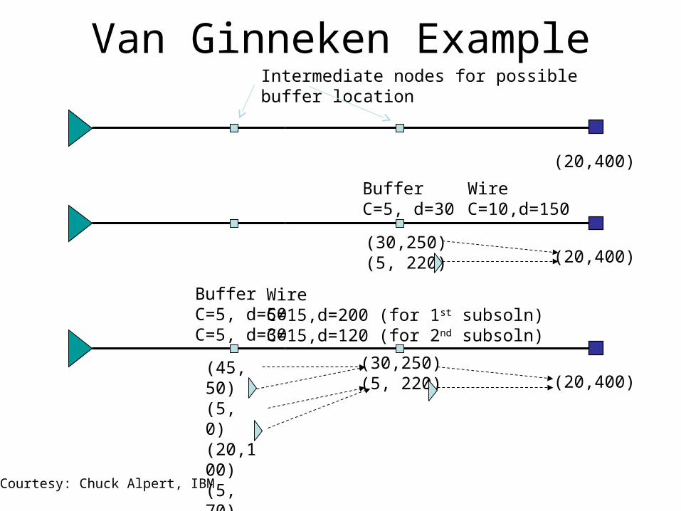
BeFS for finding an optimal TSP solution
22+9
C D E
C E D
X X X
F D
21+6C F
B F
F
A
8+16
11+14
14+9
20
5+15
• Lower-bound cost estimate: MST({unvisited cities} U {current city} U {start city})• LB as structure (spanning tree) is a superset of reqd soln structure (cycle)• min(metric M’s values in set S)<= min(M’s values in subset S’)• Similarly for max??
MST for node (A, E, F); =MST{F,A,B,C,D}; cost=16
Path cost for(A,E,F) = 8
Set S of all spanningtrees in a graph G
Set S’of all Hamiltonianpaths (that visits a nodeexactly once)in a graph G
S
S’

BFS for 0/1 ILP Solution
root(no vars
exp.)
• X = {x1, …, xm} are 0/1 vars• Choose vars Xi=0/1 as next nodes in some order (random or heuristic based)
X2=0 X2=1
Solve LPw/ x2=0;Cost=cost(LP)=C1
Solve LPw/ x2=1;Cost=cost(LP)=C2
Solve LPw/ x2=1, x4=0;Cost=cost(LP)=C3
Solve LPw/ x2=1, x4=1;Cost=cost(LP)=C4
X4=0 X4=1
X5=0 X5=1
Solve LPw/ x2=1, x4=1, x5=1Cost=cost(LP)=C6
Solve LPw/ x2=1, x4=1, x5=0Cost=cost(LP)=C5
optimal soln
Cost relations:C5 < C3 < C1 < C6C2 < C1C4 < C3
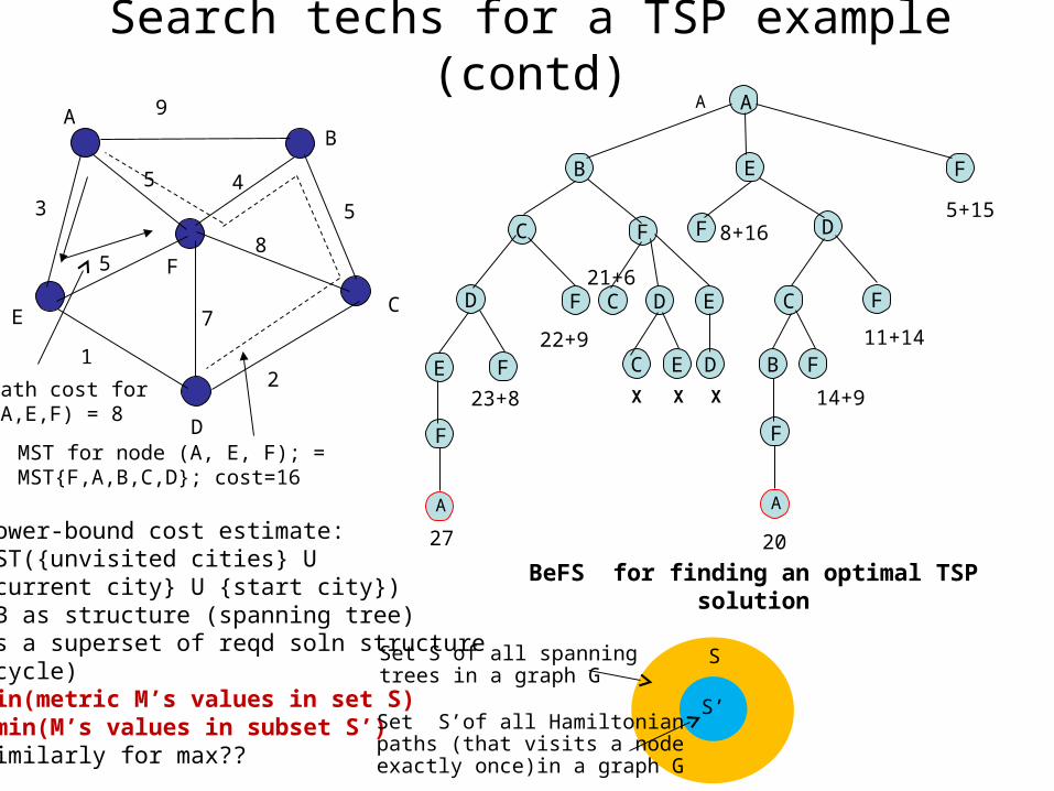
Iterative Improvement Techniques
Iterative improvement
Deterministic GreedyStochastic(non-greedy)
Locally/immediately greedy
Non-locally greedy
Make move that isimmediately (locally) bestUntil (no further impr.)(e.g., FM)
Make move that isbest according to somenon-immediate (non-local)metric (e.g., probability-based lookahead as in PROP)Until (no further impr.)
Make a combination of deterministic greedy moves and probabilistic moves that cause a deterioration (can help to jump out of local minima)Until (stopping criteria satisfied)• Stopping criteria could be an upper bound on the total # of moves or iterations