Embed Size (px)
Citation preview


Algorithmic Adventures

Juraj Hromkovic
AlgorithmicAdventures
From Knowledge to Magic

Prof. Dr. Juraj Hromkovic
ETH ZentrumDepartment of Computer ScienceSwiss Federal Institute of Technology8092 Zü[email protected]
ISBN 978-3-540-85985-7DOI 10.1007/978-3-540-85986-4
e-ISBN 978-3-540-85986-4
Springer Dordrecht Heidelberg London New York
Library of Congress Control Number: 2009926059
ACM Computing Classification (1998): K.3, A.1, K.2, F.2, G.2, G.3
c© Springer-Verlag Berlin Heidelberg 2009This work is subject to copyright. All rights are reserved, whether the whole or part of the material isconcerned, specifically the rights of translation, reprinting, reuse of illustrations, recitation, broadcasting,reproduction on microfilm or in any other way, and storage in data banks. Duplication of this publicationor parts thereof is permitted only under the provisions of the German Copyright Law of September 9,1965, in its current version, and permission for use must always be obtained from Springer. Violations areliable to prosecution under the German Copyright Law.The use of general descriptive names, registered names, trademarks, etc. in this publication does notimply, even in the absence of a specific statement, that such names are exempt from the relevant protectivelaws and regulations and therefore free for general use.
Cover design: KünkelLopka GmbH, Heidelberg
Printed on acid-free paper
Springer is part of Springer Science+Business Media (www.springer.com)

For
Urs Kirchgraber
Burkhard Monien
Adam Okruhlica
Peta and Peter Rossmanith
Georg Schnitger
Erich Valkema
Klaus and Peter Widmayer
and all those
who are fascinated
by science

Science is an innerly compact entity.Its division into different subject areasis conditioned not only by the essence of the matterbut, first and foremost, by the limitedcapability of human beings in the process of getting insight.
Max Planck
Preface
The public image of computer science does not reflect its truenature. The general public and especially high school studentsidentify computer science with a computer driving license. Theythink that studying computer science is not a challenge, and thatanybody can learn it. Computer science is not considered a sci-entific discipline but a collection of computer usage skills. Thisis a consequence of the misconception that teaching computer sci-ence is important because almost everybody possesses a computer.The software industry also behaved in a short-sighted manner, byputting too much pressure on training people in the use of theirspecific software products,
Searching for a way out, ETH Zurich offered a public lecture seriescalled The Open Class — Seven Wonders of Informatics in the fallof 2005. The lecture notes of this first Open Class were publishedin German by Teubner in 2006. Ten lectures of this Open Classform the basis of Algorithmic Adventures.

VIII Preface
The first and foremost goal of this lecture series was to show thebeauty, depth and usefulness of the key ideas in computer science.While working on the lecture notes, we came to understand thatone can recognize the true spirit of a scientific discipline only byviewing its contributions in the framework of science as a whole.We present computer science here as a fundamental science that,interacting with other scientific disciplines, changed and changesour view on the world, that contributes to our understanding ofthe fundamental concepts of science and that sheds new light onand brings new meaning to several of these concepts. We showthat computer science is a discipline that discovers spectacular,unexpected facts, that finds ways out in seemingly unsolvable sit-uations, and that can do true wonders. The message of this bookis that computer science is a fascinating research area with a bigimpact on the real world, full of spectacular ideas and great chal-lenges. It is an integral part of science and engineering with anabove-average dynamic over the last 30 years and a high degree ofinterdisciplinarity.
The goal of this book is not typical for popular science writing,which often restricts itself to outlining the importance of a researcharea. Whenever possible we strive to bring full understanding ofthe concepts and results presented. We take the readers on a voy-age where they discover fundamental computer science concepts,and we help them to walk parts of this voyage on their own andto experience the great enthusiasm of the original explorers. Toachieve this, it does not suffice to provide transparent and simpleexplanations of complex matters. It is necessary to lure the readerfrom her or his passive role and to ask her or him frequently todo some work by solving appropriate exercises. In this way wedeepen the understanding of the ideas presented and enable read-ers to solve research problems on their own.
All selected topics mark milestones in the development of com-puter science. They show unexpected turns in searching for so-lutions, spectacular facts and depth in studying the fundamen-tal concepts of science, such as determinism, causality, nonde-

Preface IX
terminism, randomness, algorithms, information, computationalcomplexity and automation.
I would like to express my deepest thanks to Yannick Born andRobin Kunzler for carefully reading the whole manuscript and fortheir numerous comments and suggestions as well as for their tech-nical support with LATEX. I am grateful to Dennis Komm for histechnical support during the work on the final version. Very spe-cial thanks go to Jela Skerlak for drawing most of the figures andto Tom Verhoeff for his comments and suggestions that were veryuseful for improving the presentation of some central parts of thisbook. The excellent cooperation with Alfred Hofmann and Ro-nan Nugent of Springer is gratefully acknowledged. Last but notleast I would like to cordially thank Ingrid Zamecnikova for herillustrations.
Zurich, February 2009 Juraj Hromkovic

Contents
1 A Short Story About the Development ofComputer Science or Why Computer Science IsNot a Computer Driving Licence . . . . . . . . . . . . . . . . 11.1 What Do We Discover Here? . . . . . . . . . . . . . . . . . . . 11.2 Fundamentals of Science . . . . . . . . . . . . . . . . . . . . . . . 21.3 The End of Euphoria . . . . . . . . . . . . . . . . . . . . . . . . . . 191.4 The History of Computer Science . . . . . . . . . . . . . . . 241.5 Summary . . . . . . . . . . . . . . . . . . . . . . . . . . . . . . . . . . . . 33
2 Algorithmics, or What Have Programming andBaking in Common? . . . . . . . . . . . . . . . . . . . . . . . . . . . . . 372.1 What Do We Find out Here? . . . . . . . . . . . . . . . . . . . 372.2 Algorithmic Cooking . . . . . . . . . . . . . . . . . . . . . . . . . . 382.3 What About Computer Algorithms? . . . . . . . . . . . . 452.4 Unintentionally Never-Ending Execution . . . . . . . . . 612.5 Summary . . . . . . . . . . . . . . . . . . . . . . . . . . . . . . . . . . . . 69
3 Infinity Is Not Equal to Infinity, or Why InfinityIs Infinitely Important in Computer Science . . . . . 733.1 Why Do We Need Infinity? . . . . . . . . . . . . . . . . . . . . 733.2 Cantor’s Concept . . . . . . . . . . . . . . . . . . . . . . . . . . . . . 773.3 Different Infinite Sizes . . . . . . . . . . . . . . . . . . . . . . . . . 1073.4 Summary . . . . . . . . . . . . . . . . . . . . . . . . . . . . . . . . . . . . 114

XII Contents
4 Limits of Computability or Why Do There ExistTasks That Cannot Be Solved Automatically byComputers . . . . . . . . . . . . . . . . . . . . . . . . . . . . . . . . . . . . . . 1174.1 Aim . . . . . . . . . . . . . . . . . . . . . . . . . . . . . . . . . . . . . . . . 1174.2 How Many Programs Exist? . . . . . . . . . . . . . . . . . . . . 1184.3 YES or NO, That Is the Question . . . . . . . . . . . . . . . 1254.4 Reduction Method . . . . . . . . . . . . . . . . . . . . . . . . . . . . 1334.5 Summary . . . . . . . . . . . . . . . . . . . . . . . . . . . . . . . . . . . . 155
5 Complexity Theory or What to Do When theEnergy of the Universe Doesn’t Suffice forPerforming a Computation? . . . . . . . . . . . . . . . . . . . . . 1615.1 Introduction to Complexity Theory . . . . . . . . . . . . . 1615.2 How to Measure Computational Complexity? . . . . . 1635.3 Why Is the Complexity Measurement Useful? . . . . . 1695.4 Limits of Tractability . . . . . . . . . . . . . . . . . . . . . . . . . 1745.5 How Do We Recognize a Hard Problem? . . . . . . . . . 1785.6 Help, I Have a Hard Problem . . . . . . . . . . . . . . . . . . . 1905.7 Summary . . . . . . . . . . . . . . . . . . . . . . . . . . . . . . . . . . . . 195
6 Randomness in Nature and as a Source ofEfficiency in Algorithmics . . . . . . . . . . . . . . . . . . . . . . . 2016.1 Aims . . . . . . . . . . . . . . . . . . . . . . . . . . . . . . . . . . . . . . . . 2016.2 Does True Randomness Exist? . . . . . . . . . . . . . . . . . . 2036.3 Abundant Witnesses Are Useful . . . . . . . . . . . . . . . . 2106.4 High Reliabilities . . . . . . . . . . . . . . . . . . . . . . . . . . . . . 2286.5 What Are Our Main Discoveries Here? . . . . . . . . . . 234
7 Cryptography, or How to Transform Drawbacksinto Advantages . . . . . . . . . . . . . . . . . . . . . . . . . . . . . . . . . 2397.1 A Magical Science of the Present Time . . . . . . . . . . 2397.2 Prehistory of Cryptography . . . . . . . . . . . . . . . . . . . . 2417.3 When Is a Cryptosystem Secure? . . . . . . . . . . . . . . . 2467.4 Symmetric Cryptosystems . . . . . . . . . . . . . . . . . . . . . 2497.5 How to Agree on a Secret in Public Gossip? . . . . . . 2537.6 Public-Key Cryptosystems . . . . . . . . . . . . . . . . . . . . . 2607.7 Milestones of Cryptography . . . . . . . . . . . . . . . . . . . . 272

Contents XIII
8 Computing with DNA Molecules, or BiologicalComputer Technology on the Horizon . . . . . . . . . . . 2778.1 The Story So Far . . . . . . . . . . . . . . . . . . . . . . . . . . . . . 2778.2 How to Transform a Chemical Lab into a DNA
Computer . . . . . . . . . . . . . . . . . . . . . . . . . . . . . . . . . . . 2828.3 Adleman’s Experiment . . . . . . . . . . . . . . . . . . . . . . . . 2888.4 The Future of DNA Computing . . . . . . . . . . . . . . . . 296
9 Quantum Computers, or Computing in theWonderland of Particles . . . . . . . . . . . . . . . . . . . . . . . . . 2999.1 Prehistory . . . . . . . . . . . . . . . . . . . . . . . . . . . . . . . . . . . 2999.2 The Wonderland of Quantum Mechanics . . . . . . . . . 3029.3 How to Compute in the World of Particles? . . . . . . 3099.4 The Future of Quantum Computing . . . . . . . . . . . . . 320
10 How to Make Good Decisions for an UnknownFuture or How to Foil an Adversary . . . . . . . . . . . . . 32510.1 What Do We Want to Discover Here? . . . . . . . . . . . 32510.2 Quality Measurement of Online Algorithms . . . . . . 32710.3 A Randomized Online Strategy . . . . . . . . . . . . . . . . . 33810.4 Summary . . . . . . . . . . . . . . . . . . . . . . . . . . . . . . . . . . . . 356
References . . . . . . . . . . . . . . . . . . . . . . . . . . . . . . . . . . . . . . . . . . 359
Index . . . . . . . . . . . . . . . . . . . . . . . . . . . . . . . . . . . . . . . . . . . . . . . 361

By living always with enthusiasm,being interested in everything that seems inaccessible,one becomes greater by striving constantly upwards.The sense of life is creativity,and creativity itself is unlimited.
Maxim Gorky
Chapter 1
A Short Story About theDevelopment of ComputerScience or Why ComputerScience Is Not a ComputerDriving Licence
1.1 What Do We Discover Here?
The goal of this chapter differs from the following chapters thateach are devoted to a specific technical topic. Here, we aim to tellthe story of the foundation of computer science as an autonomousresearch discipline in an understandable and entertaining way. Try-ing to achieve this goal, we provide some impressions about theway in which sciences develop and what the fundamental buildingblocks of computer sciences look like. In this way we get to know
J. Hromkovic, Algorithmic Adventures, DOI 10.1007/978-3-540-85986-4 1,c© Springer-Verlag Berlin Heidelberg 2009
1

2 1 The Development of Computer Science
some of the goals of the basic research in computer science as wellas a part of its overlap with other research disciplines. We also usethis chapter to introduce all ten subjects of the following chaptersin the context of the development of computer science.
1.2 Does the Building of Science Sit onUnsteady Fundamentals?
To present scientific disciplines as collections of discoveries andresearch results gives a false impression. It is even more mislead-ing to understand science merely in terms of its applications ineveryday life. What would the description of physics look like ifit was written in terms of the commercial products made possibleby applying physical laws? Almost everything created by people—from buildings to household equipment and electronic devices—is based on knowledge of physical laws. However, nobody mistakesthe manufacturer of TVs or of computers or even users of elec-tronic devices for physicists. We clearly distinguish between thebasic research in physics and the technical applications in electri-cal engineering or other technical sciences. With the exception ofthe computer, the use of specific devices has never been considereda science.
Why does public opinion equate the facility to use specific softwarepackages to computer science? Why is it that in some countriesteaching computer science is restricted to imparting ICT skills,i.e., to learning to work with a word processor or to search onthe internet? What is the value of such education, when softwaresystems essentially change every year? Is the relative complexityof the computer in comparison with other devices the only reasonfor this misunderstanding?
Surely, computers are so common that the number of car driversis comparable to the number of computer users. But why thenis driving a car not a subject in secondary schools? Soon, mobilephones will become small, powerful computers. Do we consider

1.2 Fundamentals of Science 3
introducing the subject of using mobile phones into school educa-tion? We hope that this will not be the case. We do not intend toanswer these rhetorical questions; the only aim in posing them isto expose the extent of public misunderstanding about computerscience. Let us only note that experience has shown that teachingthe use of a computer does not necessarily justify a new, specialsubject in school.
The question of principal interest to us is: “What is computerscience?” Now it will be clear that it is not about how to usea computer1. The main problem with answering this question isthat computer science itself does not provide a clear picture topeople outside the discipline. One cannot classify computer sci-ence unambiguously as a metascience such as mathematics, or asa natural science or engineering discipline. The situation wouldbe similar to merging physics and electrical and mechanical en-gineering into one scientific discipline. From the point of view ofsoftware development, computer science is a form of engineering,with all features of the technical sciences, covering the design anddevelopment of computer systems and products. In contrast, thefundamentals of computer science are closely related to mathemat-ics and the natural sciences. Computer science fundamentals playa similar role in software engineering as theoretical physics playsin electrical and mechanical engineering.
It is exactly this misunderstanding of computer science fundamen-tals among the general public that is responsible for the bad imageof computer science. Therefore we primarily devote this book toexplaining some fundamental concepts and ideas of computer sci-ence.
We already argued that the best way to understand a scientificdiscipline is not by dealing with its applications. Moreover, wesaid in the beginning that it does not suffice to view a scientificdiscipline as sum of its research results. Hence, the next principalquestions are:
“How can a scientific discipline be founded?”
1 If this were the case, then almost anybody could be considered a computer scientist.

4 1 The Development of Computer Science
“What are the fundamental building blocks of a scientific disci-pline?”
Each scientific discipline has its own language, that is, its own no-tions and terminology. Without these one cannot formulate anyclaims about the objects of interest. Therefore, the process ofevolving notions, aimed at approximating the precise meaning oftechnical terms, is fundamental to science. To establish a precisemeaning with a clear interpretation usually takes more effort thanmaking historic discoveries. Let us consider a few examples. Agree-ing on the definition of the notion “probability” took approxi-mately 300 years. Mathematicians needed a few thousand years inorder to fix the meaning of infinity in formal terms2. In physics wefrequently use the term “energy”. Maybe the cuckoo knows whatthat is, but not me. The whole history of physics can be viewed asa never-ending story of developing our understanding of this no-tion. Now, somebody can stop me and say: “Dear Mr. Hromkovic,this is already too much for me. I do not believe this. I know whatenergy is, I learnt it at school.” And then I will respond: “Do youmean the Greek definition3 of energy as a working power? Or doyou mean the school definition as the facility of a physical systemto perform work? Then, you have to tell me first, what power andwork are.” And when you start to do that, you will find that youare running in a circle, because your definition of power and workis based on the notion of energy.
We have a similar situation with respect to the notion of “life” inbiology. An exact definition of this term would be an instrumentfor unambiguously distinguishing between living and dead matter.We miss such a definition at the level of physics and chemistry.
Dear reader, my aim is not to unnerve you in this way. It is nota tragedy that we are unable to determine the precise meaningof some fundamental terms. In science we often work with defi-nitions that specify the corresponding notions only in an approx-imate way. This is everyday business for researchers. They need
2 We will tell this story in Chapter 3.3 Energy means ‘power with effects’ in Greek.

1.2 Fundamentals of Science 5
to realize that the meaning of their results cannot reach a higherdegree of precision than the accuracy of the specification of termsused. Therefore, researchers continuously strive to transform theirknowledge into the definition of fundamental notions in order toget a better approximation of the intended meaning. An excellentexample of progress in the evolution of notions, taken from thehistory of science, is the deepening of our understanding of thenotion of “matter”.
To understand what it takes to define terms and how hard thiscan be, we consider the following example. Let us take the word“chair”. A chair is not an abstract scientific object. It is simply acommon object and most of us know or believe we know what itis. Now, please try to define the term “chair” by a description.
To define a term means to describe it in such an accurateway that, without having ever seen a chair and followingonly your description, anybody could unambiguously decidewhether a presented object is a chair or not. In your defini-tion only those words are allowed whose meaning has alreadybeen fixed.
The first optimistic idea may be to assume that one already knowswhat a leg of a piece of furniture is. In this case, one could startthe definition with the claim that a chair has four legs. But halt.Does the chair you are sitting on have four legs? Perhaps it onlyhas one leg, and moreover this leg is a little bit strange4? Let it be!My aim is not to pester you. We only want to impress upon youthat creating notions is not only an important scientific activity,but also very hard work.
We have realized that creating notions is a fundamental topic ofscience. The foundation of computer science as a scientific disci-pline is also related to building a notion, namely that of “algo-rithm”. Before we tell this story in detail, we need to know aboutaxioms in science.4 In the lecture room of OpenClass, there are only chairs with one leg in the formof the symbol “L” and the chair is fixed on a vertical wall instead of on the floor.

6 1 The Development of Computer Science
Axioms are the basic components of science. They arenotions, specifications, and facts, about whose validity andtruth we are strongly convinced, though there does not existany possibility of proving their correctness.
At first glance, this may look strange, even dubious. Do we wantto doubt the reliability of scientific assertions? Let us explain thewhole by using an example. One such axiom is the assumption thatwe think in a correct way, and so our way of arguing is reliable.Can we prove that we think correctly? How? Using our arguments,which are based on our way of thinking? Impossible. Hence, noth-ing else remains than to trust in our way of thinking. If this axiomis not true, then the building of science will collapse. This axiom isnot only a philosophical one, it can be expressed in a mathemati-cal way. And since mathematics is the formal language of science,one cannot do anything without it.
Let us carefully explain the exact meaning of this axiom.
If
an event or a fact B is a consequence of another event orfact A,
then the following must hold:
if A holds (if A is true),then B holds (then B is true).
In other words,
untruthfulness cannot be a consequence of truth.
In mathematics one uses the notation
A ⇒ B
for the fact
B is a consequence of A.
We say also
A implies B.

1.2 Fundamentals of Science 7
Using this notation, the axiom says: If
both A ⇒ B, and A hold,
then
B holds.
We call attention to the fact that it is allowed that an untruthimplies a truth. The only scenario not permitted is that untruth(falsehood) is a consequence of truth. To get a deeper understand-ing of the meaning of this axiom, we present the following example.
Example 1.1 We consider the following two statements A andB:
A is “It is raining”
and
B is “The meadow is wet”.
We assume that our meadow is in the open air (not covered).Hence, we may claim that the statement
“If it is raining, then the meadow is wet”
i.e.,
A ⇒ B
holds.
Following our interpretation of the terms “consequence” and “im-plication”, the meadow must be wet (i.e., B holds) when it israining (i.e., when A holds). Let us look at this in detail.
“A holds” means “it is raining”.“A does not hold” means “it is not raining”.“B holds” means “the meadow is wet”.“B does not hold” means “the meadow is dry”.
With respect to the truth of A and B, there are the following fourpossible situations:

8 1 The Development of Computer Science
S1: It is raining and the meadow is wet.S2: It is raining and the meadow is dry.S3: It is not raining and the meadow is wet.S4: It is not raining and the meadow is dry.
Usually, scientists represent these four possibilities in a so-calledtruth table (Fig. 1.1)
A B
S1 true true
S2 true false
S3 false true
S4 false false
Fig. 1.1: Truth table for A and B
Mathematicians like to try to write everything as briefly as pos-sible and unfortunately they do it even when there is a risk thatthe text essentially becomes less accessible for nonspecialists. Theyrepresent truth by 1 and falsehood (untruth) by 0. Using this no-tation, the size of the truth table in Fig. 1.1 can be reduced to thesize of the table in Fig. 1.2.
A B
S1 1 1
S2 1 0
S3 0 1
S4 0 0
Fig. 1.2: Truth table for A and B (short version)
It is important to observe that the truth of the implication A ⇒ Bexcludes the situation S2 in the second row (A is true and B isfalse) only. Let us analyze this in detail.
The first row corresponds to the situation S1, in which both A andB hold. This means it is raining and consequently the meadow iswet. Clearly, this corresponds to the validity of A ⇒ B and soagrees with our expectation.

1.2 Fundamentals of Science 9
The second row with “A holds” and “B does not hold” corre-sponds to the situation when it is raining and the meadow is dry.This situation is impossible and contradicts the truthfulness of ourclaim A ⇒ B, because our understanding of “A ⇒ B” means thatthe validity of A (“it is raining”) demands the validity of B (“themeadow is wet”).
The third row describes the situation S3 in which it is not raining(A is false) and the meadow is wet (B is true). This situationis possible and the fact A ⇒ B does not exclude this situation.Despite the first fact that it is not raining, the meadow can be wet.Maybe it was raining before or somebody watered the meadow. Orin the early morning after a cold night the dew is on the grass.
The last row (both A and B do not hold) corresponds to thesituation in which it is not raining and the meadow is dry. Clearly,this situation is possible and does not contradict the validity ofthe claim A ⇒ B either.
We summarize our observations. If A ⇒ B holds and A holds (“itis raining”), then B (“the meadow is wet”) must hold too. If Adoes not hold (“it is not raining”), then the validity of A ⇒ Bdoes not have any consequences for B and so B may be true orfalse (rows 3 and 4 in the truth table). �When A ⇒ B is true, the only excluded situation is
“A holds and B does not hold”.
If one has a truth table for two claims A and B, in which allsituations with respect to the truthfulness of A and B are possible,except the situation “A holds and B does not hold”, then one cansay that A ⇒ B holds. From the point of view of mathematics,the truth table in Fig. 1.3 is the formal definition of the notion of“implication”.
In this way, we have the following simple rule for recognizing andfor verifying the validity of an implication A ⇒ B.

10 1 The Development of Computer Science
A B A ⇒ B
true true possible (true)
true false impossible (false)
false true possible (true)
false false possible (true)
Fig. 1.3: Definition of the implication
If in all possible situations (in all situations that may occur)in which A is true (holds), B is also true (holds), then A ⇒B is true (holds).
Exercise 1.1 Consider the following two statements A and B. A means: “It iswinter” and B means “The brown bears are sleeping”. The implication A ⇒ Bmeans:
“If it is winter, then the brown bears are sleeping.”
Assume the implication A ⇒ B holds. Create the truth table for A and B andexplain which situations are possible and which ones are impossible.
Now, we understand the meaning of the notion of implication (ofconsequence). Our next question is the following one:
What have the implication and correct argumentation incommon? Why is the notion of implication the basis forfaultless reasoning or even for formal, mathematical proofs?
We use the notion of implication for the development of so-calleddirect argumentation (direct proofs) and indirect argumentation(indirect proofs). These two argumentation methods form the ba-sic instrument for faultless reasoning. In order to make our argu-mentations in the rest of the book transparent and accessible foreverybody, we introduce these two basic proof methods in whatfollows.
Consider our statements A (“It is raining”) and B (“The meadowis wet”) from Example 1.1. Consider additionally a new statementC saying that the salamanders are happy. We assume that A ⇒ Bholds and moreover that
B ⇒ C (“If the meadow is wet, then the salamanders arehappy”)

1.2 Fundamentals of Science 11
holds too. What can be concluded from that? Consider the truthtable in Fig. 1.4 that includes all 8 possible situations with respectto the validity of A, B, and C.
A B C A ⇒ B B ⇒ C
S1 true true true
S2 true true false impossible
S3 true false true impossible
S4 true false false impossible
S5 false true true
S6 false true false impossible
S7 false false true
S8 false false false
Fig. 1.4: Truth table for A ⇒ B, B ⇒ C
Since A ⇒ B is true, the situations S3 and S4 are excluded (impos-sible). Analogously, the truth of B ⇒ C excludes the possibility ofthe occurrence of the situations S2 and S6. Let us view this tablefrom the point of view of A and C only. We see that the followingsituations are possible:
(i) both A and C hold (S1)
(ii) both A and C do not hold (S8)
(iii) A does not hold and C holds (S5, S7).
The situations S2 and S4 in which A holds and C does not holdare excluded because of A ⇒ B and B ⇒ C. In this way we obtain
A ⇒ C (“If it is raining, then the salamanders are happy”)
is true.
The implication A ⇒ C is exactly what one would expect. If itis raining, then the meadow must be wet (A ⇒ B), and if themeadow is wet then the salamanders must be happy (B ⇒ C).Hence, through the wetness of the meadow, the rain causes thehappiness of the salamanders (A ⇒ C).

12 1 The Development of Computer Science
The argument
“If A ⇒ B and B ⇒ C are true,then A ⇒ C is true”
is called a direct proof (direct argument). Direct proofs may bebuilt from arbitrarily many implications. For instance, the truthof the implications
A1 ⇒ A2, A2 ⇒ A3, A3 ⇒ A4, . . . , Ak−1 ⇒ Ak
allows us to conclude that
A1 ⇒ Ak
holds. From this point of view, direct proofs are simply sequencesof correct implications. In mathematics lessons, we perform manydirect proofs in order to prove various statements. Unfortunately,mathematics teachers often forget to express this fact in a trans-parent way and therefore we present here a small example from amathematics lesson.
Example 1.2 Consider the linear equality 3x − 8 = 4. Our aimis to prove that
x = 4 is the only solution of the equality 3x − 8 = 4.
In other words we aim to show the truth of the implication
“If 3x − 8 = 4 holds, then x = 4”.
Let A be the statement “The equality 3x−8 = 4 holds” and let Zbe the statement “x = 4 holds”. Our aim is to prove that A ⇒ Zholds. To do it by direct proof, we build a sequence of undoubtedlycorrect implications starting with A and finishing with Z.
We know that an equality5 remains valid if one adds the samenumber to both sides of the equality. Adding the integer 8 to bothsides of the equality 3x − 8 = 4, one obtains
5 To be precise, the solutions of an equality do not change if one adds the samenumber to both sides of the equality.

1.2 Fundamentals of Science 13
3x − 8 + 8 = 4 + 8
and consequently
3x = 12.
Let B be the assertion that the equality 3x = 12 holds. Above weshowed the truthfulness of the implication A ⇒ B (“If 3x− 8 = 4is true, then 3x = 12 is true”).
Thus, we have already our first implication. We also know that anequality remains valid if one divides both sides of the equality bythe same nonzero number. Dividing both sides of 3x = 12 by 3,we obtain
3x
3=
12
3
and so
x = 4.
In this way we get the truthfulness of the implication B ⇒ Z (“Ifthe equality 3x = 12 holds, then the equality x = 4 holds”).
The validity of the implications A ⇒ B and B ⇒ Z allows us toclaim that A ⇒ Z holds. Hence, if 3x − 8 = 4 holds, then x = 4.One can easily verify that x = 4 satisfies the equality. Thus, x = 4is the only solution of the equality 3x − 8 = 4. �Exercise 1.2 Show by direct argumentation (through a sequence of implications)that x = 1 is the only solution of the equality 7x − 3 = 2x + 2.
Exercise 1.3 Consider the truth table for the three statements A, B, and C inFig. 1.5.
We see that only 3 situations (S1, S2, and S8) are possible and all others are impos-sible. Which implications hold? For instance, the implication C ⇒ A holds, becausewhenever in a possible situation C is true, then A is true too. The implication B ⇒ Cdoes not hold, because in the possible situation S2 it happens that B holds and Cdoes not hold. Do you see other implications that hold?

14 1 The Development of Computer Science
A B C
S1 1 1 1
S2 1 1 0
S3 1 0 1 impossible
S4 1 0 0 impossible
S5 0 1 1 impossible
S6 0 1 0 impossible
S7 0 0 1 impossible
S8 0 0 0
Fig. 1.5: Truth table for A, B and C in Exercise 1.3
Most of us rarely have troubles understanding the concept of di-rect argumentation. On the other hand indirect argumentation isconsidered to be less easily understood. Judging whether indirectargumentation is really more complex than direct argumentation,and to what extent the problem arises because of poor didactic ap-proaches in schools is left to the reader. Since we apply indirect ar-gumentation for discovering some fundamental facts in Chapters 3and 4, we take the time to explain the schema of this reasoning inwhat follows.
Let us continue with our example. The statement A means “Itis raining”, B means “The meadow is wet”, and C means “Thesalamanders are happy”. For each statement D, we denote by Dthe opposite of D. In this notation, A means “It is not raining”,B means “The meadow is dry”, and C means “The salamandersare unhappy”. Assume, as before, that the implications A ⇒ Band B ⇒ C hold.
Now, suppose we or the biologists recognize that
“The salamanders are unhappy”
i.e., that C holds (C does not hold). What can one conclude fromthat?
If the salamanders are unhappy, the meadow cannot be wet, be-cause the implication B ⇒ C guarantees the happiness of thesalamanders in a wet meadow. In this way one knows with cer-tainty that B holds. Analogously, the truthfulness of B and of

1.2 Fundamentals of Science 15
the implication A ⇒ B implies that it is not raining, because inthe opposite case the meadow would be wet. Hence, A holds. Weobserve in this way that the validity of
A ⇒ B, B ⇒ C, and C
implies the validity of
B and A.
We can observe this argumentation in the truth table in Fig. 1.6too. The validity of A ⇒ B excludes the situations S3 and S4.Since B ⇒ C holds, the situations S2 and S6 are impossible.
A B C A ⇒ B B ⇒ C C does not hold
S1 true true true impossible
S2 true true false impossible
S3 true false true impossible impossible
S4 true false false impossible
S5 false true true impossible
S6 false true false impossible
S7 false false true impossible
S8 false false false
Fig. 1.6: Truth table for A, B and C
Since C holds (since C does not hold), the situations S1, S3, S5,and S7 are impossible. Summarizing, S8 is the only situation thatis possible. The meaning of S8 is that none of the statements A, B,and C holds, i.e., that all of A, B, and C are true. Thus, startingfrom the validity of A ⇒ B, B ⇒ C, and C, one may concludethat B, and C hold.
Exercise 1.4 Consider the statements A, B, and C with the above meaning. As-sume A ⇒ B, B ⇒ C and B hold. What can you conclude from that? Depict thetruth table for all 8 situations with respect to the validity of A, B, and C anddetermine which situations are possible when A ⇒ B, B ⇒ C and B hold.
We observe that the validity of A ⇒ B, B ⇒ C, and C doesnot help to say anything about the truthfulness of A and B. IfC holds, the salamanders are happy. But this does not mean thatthe meadow is wet (i.e., that B holds). The salamanders can also

16 1 The Development of Computer Science
have other reasons to be happy. A wet meadow is only one of anumber of possible reasons for the happiness of the salamanders.
Exercise 1.5 Depict the truth table for A, B, and C, and determine which situa-tions are possible when A ⇒ B, B ⇒ C, and C are true.
Exercise 1.6 Consider the following statements C and D. C means “The coloryellow and the color blue were mixed”, and D means “The color green is created”.The implication C ⇒ D means:
“If one mixed the color yellow with blue, then the color green is created.”
Assume that C ⇒ D holds. Depict the truth table for C and D and explain whichsituations are possible and which are impossible. Can you conclude from the validityof C ⇒ D the validity of the following statement?
“If the created color differs from green, then the color yellow was not mixedwith the color blue.”
Slowly but surely, we are starting to understand the schema ofindirect argumentation. Applying the schema of the direct proof,we know that a statement A holds and we aim to prove the validityof a statement Z. To do this, we derive a sequence of correctimplications
A ⇒ A1, A1 ⇒ A2, . . . , Ak−1 ⇒ Ak, Ak ⇒ Z
that guarantees us the validity of A ⇒ Z. From the validity of Aand of A ⇒ Z we obtain the truthfulness of Z.
The schema of an indirect proof can be expressed as follows.
Initial situation: We know that a statement D holds.Aim: To prove that a statement Z holds.
We start from Z as the opposite of Z and derive a sequence ofcorrect implications
Z ⇒ A1, A1 ⇒ A2, . . . , Ak−1 ⇒ Ak, Ak ⇒ D.
This sequence of implications ends with D that clearly does nothold, because we assumed that D holds.
From this we can conclude that Z does not hold, i.e. that Z as theopposite of Z holds.

1.2 Fundamentals of Science 17
The correctness of this schema can be checked by considering thetruth table in Fig. 1.7.
D Z D Z Z ⇒ D D holds
S1 true true false false
S2 true false false true impossible
S3 false true true false impossible
S4 false false true true impossible
Fig. 1.7: Truth table for D and Z
The situation S2 is impossible, because Z ⇒ D holds. Since Dholds6, the situations S3 and S4 are impossible. In the only re-maining situation S1 the statement Z is true, and so we haveproved the aimed validity of Z.
This proof method is called indirect, because in the chain of im-plications we argue in the opposite direction (from the end to thebeginning). If D does not hold (i.e., if D holds), then Z cannothold and so Z holds.
In our example we had D = C, i.e., we knew that the salamandersare not happy. We wanted to prove that the consequence is thatit is not raining, i.e., our aim was to show that Z = A holds.Expressing the implications
A ⇒ B, B ⇒ C
in our new notation one obtains
Z ⇒ B, B ⇒ D.
From the validity of Z ⇒ D and D, we were allowed to concludethat the opposite of Z = A must hold. The opposite of Z is Z = A.Hence, we have proved that it is not raining (i.e., that A holds).
The general schema of the indirect proofs is as follows. One wantsto prove the truth of a statement Z. We derive a chain of impli-cations
6 This was our starting point.

18 1 The Development of Computer Science
Z ⇒ A1, A1 ⇒ A2, . . . , Ak ⇒ U ,
which in turn provides
Z ⇒ U ,
i.e., that Z as the opposite of our aim Z implies a nonsense U .Since the nonsense U does not hold, the statement Z does nothold, too. Hence, Z as the opposite of Z holds.
Exercise 1.7 Let x2 be an odd integer. We want to give an indirect proof that thenx must be an odd integer, too. We use the general schema for indirect proofs. Let Abe the statement that “x2 is odd” and let Z be the statement that “x is odd”. Ouraim is to prove that Z holds, if A is true. One can prove the implication Z ⇒ A byshowing that for each even number 2i
(2i)2 = 22i2 = 4i2 = 2(2i2)
and so (2i)2 is an even number. Complete the argumentation of this indirect proof.
Exercise 1.8 Let x2 be an even integer. Apply the schema of indirect proofs inorder to show that x is even.
Exercise 1.9 (Challenge) Prove by an indirect argument that√
2 is not a rationalnumber. Note that rational numbers are defined as numbers that can be expressedas fractions of integers.
In fact, one can view the axioms of correct argumentation as cre-ating the notion of implication in a formal system of thinking.Usually, axioms are nothing other than fixing the meaning of somefundamental terms. Later in the book, we will introduce the defi-nition of infinity that formalizes and fixes our intuition about themeaning of the notion of infinity. Clearly, it is not possible to provethat this definition exactly corresponds to our intuition. But thereis a possibility of disproving an axiom. For instance, one finds anobject, that following our intuition, has to be infinite but withrespect to our definition it is not. If something like this happens,then one is required to revise the axiom.
A revision of an axiom or of a definition is not to be viewed as adisaster or even as a catastrophe. Despite the fact that the changeof a basic component of science may cause an extensive reconstruc-tion of the building of science, we view the revision as a pleasing

1.3 The End of Euphoria 19
event because the resulting new building of science is more stableand so more reliable.
Up till now, we spoke about basic components of science only.What can be said about those components that are above thebase? Researchers try to build science carefully, in such a waythat the correctness of the axioms (basic components) assures thecorrectness of the whole building of science. Especially mathemat-ics is systematically created in this way. This is the well-knownobjectivity and reliability of science. At least in mathematics andsciences based on arguments of mathematics the truthfulness ofaxioms implies the validity of all results derived.
1.3 Origin of Computer Science as the End ofEuphoria
At the end of the nineteenth century, society was in a euphoricstate in view of the huge success of science, resulting in the tech-nical revolution that transformed knowledge into the ability todevelop advanced machines and equipment. The products of thecreative work of scientists and engineers entered into everyday lifeand essentially increased the quality of life. The unimaginable be-came reality. The resulting enthusiasm of scientists led not only tosignificant optimism, but even to utopian delusions about man’scapabilities. The image of the causal (deterministic) nature of theworld was broadly accepted. People believed in the existence of anunambiguous chain of causes and their effects like the followingone
cause1 ⇒ effect1
effect1 = cause2
cause2 ⇒ effect2
effect2 = cause3
cause3 ⇒ . . .
and attempted to explain the functioning of the world in theseterms. One believed that man is able to discover all laws of nature

20 1 The Development of Computer Science
and that this knowledge suffices for a complete understanding ofthe world. The consequence of this euphoria in physics was thatone played the Gedankenexperiment in which one believes in theexistence of so-called demons, who are able to calculate and so pre-dict the future. Physicists were aware of the fact that the universeconsists of a huge number of particles and that nobody is ableto record the positions and the states of all of them at a singlemoment in time. Therefore, they knew that knowing all the lawsof nature does not suffice for a man to predict the future. Hence,physicists introduced the so-called demons as superhumans able torecord the description of the state of the whole universe (the statesof all particles and all interactions between them). Knowing all thelaws of nature, the hypothetical demon has to be able to calculateand so to predict the future. I do not like this idea and do not con-sider it to be optimistic, because it means that the future is alreadydetermined. Where then is place for our activities? Are we unableto influence anything? Are we in the best case only able to predictthis unambiguously determined future? Fortunately, physics itselfsmashed this image. First, chaos theory showed that there existsystems such that an unmeasurably small change in their statescauses a completely different development in their future. Thisfact is well known as the so-called butterfly effect. The final rea-son for ending our belief in the existence of demons is related to thediscovery of the laws of quantum mechanics7 that became a funda-ment of correct physics. Quantum mechanics is based on genuinelyrandom, hence unpredictable, events that are a crucial part of thelaws governing the behavior of particles. If one accepts this the-ory (up to now, no contradiction has ever been observed betweenthe predictions of quantum mechanics and the experiments tryingto verify them), then there does not exist any unambiguously de-termined future and so there is some elbow room for shaping thefuture.
The foundation of computer science is related to another “unre-alistic” delusion. David Hilbert, one of the most famous mathe-
7 We provide more information about this topic in Chapter 6 on randomness and inChapter 9 on quantum computing.

1.3 The End of Euphoria 21
maticians, believed in the existence of a method for solving allmathematical problems. More precisely, he believed
(i) that all of mathematics can be created by starting from a finitecollection of suitable axioms,
(ii) that mathematics created in this way is complete in the sensethat every statement expressible in the language of mathemat-ics can be either proved or disproved in this theory,
(iii) and that there exists a method for deciding the correctness ofany statement.
The notion of “method” is crucial for our consideration now. Whatwas the understanding of this term at that time?
A method for solving a problem (a task) describes an effec-tive path that leads to the problem solution. This descriptionmust consist of a sequence of instructions that everybody canperform (even people who are not mathematicians).
The main point is to realize that one does not need to understandwhy a method works and how it was discovered in order to be ableto apply it for solving given problem instances. For instance, con-sider the problem of solving quadratic equations of the followingform:
x2 + 2px + q = 0
If p2 − q ≥ 0, then the formulae
x1 = −p +√
p2 − q
x2 = −p −√
p2 − q
describe the calculation of the two solutions of the given quadraticequation. We see that one can compute x1 and x2 without anyknowledge about deriving these formulae and so without under-standing why this way of computing solutions to quadratic equa-tion works. One only needs the ability to perform arithmetic op-erations. In this way, a computer as a machine without any intel-ligence can solve quadratic equations by applying this method.

22 1 The Development of Computer Science
Therefore, one associates the existence of a mathematical methodfor solving a problem to the possibility of calculating solutions inan automatic way. Today, we do not use the notion “method”in this context, because this term is used in many different areaswith distinct meanings. Instead, we use the term algorithm. Thechoice of this new term as a synonym for a solution method wasinspired by the name of the Arabic mathematician al-Khwarizmi,who wrote a book about algebraic methods in Baghdad in theninth century. Considering this interpretation of the notion of al-gorithm, David Hilbert strove to automate the work of mathe-maticians. He strove to build a perfect theory of mathematics inwhich one has a method for verifying the correctness of all state-ments expressible in terms of this mathematics. In this theory, themain activity of mathematicians devoted to the creation of proofswould be automated. In fact, it would be sad, if creating correctargumentations—one of the hardest intellectual activities—couldbe performed automatically by a dumb machine.
Fortunately, in 1931, Kurt Godel definitively destroyed all dreamsof building such a perfect mathematics. He proved by mathemati-cal arguments that a complete mathematics, as desired by Hilbert,does not exist and hence cannot be created. Without formulatingthese mathematical theorems rigorously, we present the most im-portant statement in an informal way:
(a) There does not exist any complete, “reasonable” mathematicaltheory. In each correct and sufficiently “large” mathematicaltheory (such as current mathematics) one can formulate state-ments, whose truthfulness cannot be verified inside this theory.To prove the truthfulness of such theorems, one must add newaxioms and so build a new, even larger theory.
(b) A method (algorithm) for automatically proving mathematicaltheorems does not exist.
If one correctly interprets the results of Godel, one realizes thatthis message is a positive one. It says that building mathematicsas a formal language of science is an infinite process. Inserting anew axiom means adding a new word (building a new notion) to

1.3 The End of Euphoria 23
our vocabulary. In this way, on one side the expressive power ofthe language of science grows, and on the other hand the powerof argumentation grows, too. Due to new axioms and the relatednew terms, we can formulate statements about objects and eventswe were not able to speak about before. And we can verify thetruthfulness of assertions that were not checkable in the old theory.Consequently, the verification of the truthfulness of statementscannot be automated.
The results of Godel have changed our view on science. We un-derstand the development of science more or less as the processof developing notions and of discovering methods. Why were theresults of Godel responsible for the founding of computer science?Here is why. Before Godel nobody saw any reason to try and givean exact definition of the notion of a method. Such a definitionwas not needed, because people only presented methods for solv-ing particular problems. The intuitive understanding of a methodas an easily comprehensible description of a way of solving a prob-lem was sufficient for this purpose. But when one wanted to provethe nonexistence of an algorithm (of a method) for solving a givenproblem, then one needed to know exactly (in the sense of a rigor-ous mathematical definition) what an algorithm is and what it isnot. Proving the nonexistence of an object is impossible if the ob-ject has not been exactly specified. First, we need to know exactlywhat an algorithm is and then we can try to prove that, for someconcrete problems, there do not exist algorithms solving them. Thefirst formal definition of an algorithm was given by Alan Turingin 1936 and later further definitions followed. The most importantfact is that all reasonable attempts to create a definition of the no-tion of algorithm led to the same meaning of this term in the senseof specifying the classes of automatically (algorithmically) solvableproblems and automatically unsolvable problems. Despite the factthat these definitions differ in using different mathematical ap-proaches and formalisms, and so are expressed in different ways,the class of algorithmically solvable problems determined by themis always the same. This confirmed the belief in the reasonability

24 1 The Development of Computer Science
of these definitions and resulted in viewing Turing’s definition ofan algorithm as the first8 axiom9 of computer science.
Now, we can try to verify our understanding of axioms once again.We view the definition of an algorithm as an axiom, because it isimpossible to prove its truthfulness. How could one prove that ourrigorous definition of algorithmic solvability really corresponds toour intuition, which is not rigorous? We cannot exclude the possi-bility of a refutation of this axiom. If somebody designs a methodfor a special purpose and this method corresponds to our intuitiveimage of an algorithm, but is not an algorithm with respect toour definition, then the definition was not good enough and wehave to revise it. In spite of many attempts to revise the definitionof an algorithm since 1936, each attempt only confirmed Turing’sdefinition and so the belief in this axiom grew. After proving thatthe class of problems algorithmically solvable by quantum com-puters is the same as the class of problems solvable by Turing’salgorithms, almost nobody sees any possibility of a violation ofthis axiom.
The notion of an algorithm is so crucial for computer science thatwe do not try to explain its exact meaning in a casual mannernow. Rather, we devote a whole chapter of this book to buildingthe right understanding of the notions of an algorithm and of aprogram.
1.4 The History of Computer Science and theConcept of This Book
The first fundamental question of computer science is the followingone:
8 All axioms of mathematics are considered axioms of computer science, too.9 More precisely, the axiom is the claim that Turing’s definition of an algorithmcorresponds to our intuitive meaning of the term “algorithm”.

1.4 The History of Computer Science 25
Do there exist tasks (problems) that cannot be solved au-tomatically (algorithmically)? And, if yes, which tasks arealgorithmically solvable and which are not?
We aim not only to answer these questions, but we attempt topresent the history of discovering the right answers in such a waythat, following it, anybody could fully understand the correctnessof these answers in detail. Since this topic is often considered tobe one of the hardest subjects of the first two years of computerscience study at university, we proceed towards our aim in a se-quence of very small steps. Therefore, we devote to this oldest partof computer science history three whole chapters.
The second chapter is titled as follows:
“Algorithmics, or What Do Programming and Baking Havein Common?”
It is primarily devoted to developing and understanding the keynotions of an algorithm and of a program. To get a first idea ofthe meaning of these terms, we start with baking a cake.
Have you ever baked a cake following a recipe? Or have you cookeda meal without any idea why the recipe asks you to work in theprescribed way? During the cooking you were aware of the fact thatthe correct performance of every step is enormously important forthe quality of your final product. What did you discover? If youare able to follow the detailed instructions of a well-written recipecorrectly, then you can be very successful in cooking without beingan expert. Even if, with considerable euphoria, we may think for amoment we are masters in cooking, we are not necessarily excellentcooks. One can become a good cook only if one grasps the deeperrelations between the product and the steps of its production, andcan write down the recipes.
The computer has a harder life. It can perform only a few verysimple activities (computation steps), in contrast to instructionspresent in recipes, such as mixing two ingredients or warming thecontent of a jar. But the main difference is that the computer doesnot have any intelligence and therefore is unable to improvise. A

26 1 The Development of Computer Science
computer cannot do anything other than follow consistently stepby step the instructions of its recipe, which is its program. It doesnot have any idea about what complex information processing itis doing.
In this way, we will discover that the art of programming is towrite programs as recipes that make methods and algorithms “un-derstandable” for computers in the sense that, by executing theirprograms, computers are able to solve problems. To realize thisproperly, we introduce a model of a computer, and show which in-structions it can execute, and what happens when it is executingan instruction. In doing so, we also learn what algorithmic prob-lems and tasks are and what the difference is between the termsalgorithm and program.
The title of the third chapter is
“Infinity Is Not Equal to Infinity, or Why Is Infinity In-finitely Important for Computer Scientists?”
This chapter is fully devoted to infinity. Why does one consider theintroduction of the notion of “infinity” to be not only useful, but tobe extremely important and even indispensable for understandingthe functioning of our finite world?
The whole new universe is huge, but finite. Everything we see, ev-erything we experiment with, and everything we can influence isfinite. No one has ever been in touch with anything infinite. Nev-ertheless, mathematics and computer science, and therefore manyother scientific disciplines are unable to exist without infinity. Al-ready in the first class of elementary school, we meet the naturalnumbers 0, 1, 2, 3, 4, . . . which are infinitely many.
Why does one need infinitely many numbers, when the number ofall particles in the universe is a big, but still a concrete number?Why do we need larger numbers? What meaning does infinityhave in computer science and how is it related to the limits of theautomatically doable?

1.4 The History of Computer Science 27
Striving to answer these questions, we will learn not only the math-ematical definition of infinity, but in addition we will see why theconcept of infinity is useful. We will realize that the, at first glance,artificial notion of infinity turns out to be a successful, power-ful and even irreplaceable instrument for investigating our finiteworld.
In Chapter 4, titled
“Computability, or Why Do There Exist Tasks That CannotBe Solved by Any Computer Controlled by Programs?”
we first apply our knowledge about infinity to show the existenceof tasks that are not algorithmically (automatically) solvable.
How can one prove the algorithmic unsolvability of concrete tasksand problems that are formulated in real life? We apply the re-duction method, which is one of the most powerful and most suc-cessful tools of mathematics for problem solving. It was originallydesigned for getting positive results, and we use it here in a rathersurprising way. We modify this method to get an instrument forproducing and propagating negative results about algorithmic un-solvability of problems. In this way, we are able to present severalwell-motivated problems that cannot automatically be solved bymeans of information technology (computers). With that, the firstkey goal of our book—proving the existence of algorithmically un-solvable problems—is reached.
In the early 1960s, after researchers successfully developed a theoryfor classifying problems into automatically solvable and unsolv-able ones, computers started to be widely used in industry. Whenapplying algorithms for solving concrete problems, the questionof their computational complexity and so of their efficiency be-came more central than the question of the existence of algorithms.Chapter 5 is devoted to the notions and concepts of complexitytheory and is titled
“Complexity Theory, or What Can One Do, If the Energyof the Whole Universe Is Insufficient to Perform a Compu-tation?”

28 1 The Development of Computer Science
After the notion of an algorithm, the notion of complexity is thenext key notion of computer science. ‘Complexity’ is understood,in computer science, as the amount of work a computer does whencalculating a solution. Typically, this is measured by the numberof computer operations (instructions) performed or the amount ofmemory used. We will also try to measure the intrinsic complexityof problems. We do so by considering the complexity of the fastest(or of the best in another sense) algorithm for solving this problem.
The main goal of complexity theory is to classify problems (algo-rithmic tasks) into easy and hard with respect to their computa-tional complexity. We know that the computational complexity ofproblems may be arbitrarily high and so that there exist very hardproblems. We know several thousand problems from practice, forwhich the best algorithms for solving them have to execute moreoperations than the number of protons in the universe. Neitherthe energy of the whole universe, nor the time since the Big Bangis sufficient to solve them. Does there exist a possibility to try atleast something with such hard problems?
Here we outline the first miracle of computer science. There areseveral promising possibilities for attacking hard problems. Andhow to do so is the proper art of algorithmics. Many hard problemsare in the following sense unstable or sensitive. A small change inthe problem formulation or a small reduction in our requirementscan cause a huge jump from an intractable amount of computerwork to a matter of a few seconds on a common PC. How to obtainsuch effects is the topic of the chapters ahead.
The miracles occur when our requirements are reduced so slightlythat this reduction (almost) does not matter in the applicationsconsidered, although it saves a huge amount of computer work.
The most magical effects are caused by using randomized control.The surprises are so fascinating as to be true miracles. Therefore,we devote a whole chapter to the topic of randomization:
“Randomness and Its Role in Nature, or Randomness as aSource of Efficiency in Algorithmics”

1.4 The History of Computer Science 29
The idea is to escape the deterministic control flow of programsand systems by allowing algorithms to toss a coin. Depending onthe outcome (heads or tails), the algorithm may choose differentstrategies for searching for a solution. This way, one sacrifices ab-solute reliability in the sense of the guarantee to always computea correct solution, because one allows some sequences of randomevents (coin tosses) to execute unsuccessful computations. An un-successful computation may be a computation without any resultor even a computation with a false result. But if one can reducethe probability of executing an unsuccessful computation to onein a billion, then the algorithm may be very useful.
We call attention to the fact that in practice randomized algo-rithms with very small error probabilities can even be more reliablethan their best deterministic counterparts. What do we mean bythis? Theoretically, all deterministic programs are absolutely cor-rect, and randomized ones may err. But the nature of the story isthat the execution of deterministic programs is not absolutely reli-able, because during their runs on a computer the probability of ahardware error grows proportionally with the running time of theprogram. Therefore a fast randomized algorithm can be more re-liable than a slow deterministic one. For instance, if a randomizedprogram computes a result in 10 seconds with an error probabil-ity 10−30, then it is more reliable than a deterministic programthat computes the result in 1 week. Hence, using randomization,one can obtain phenomenal gains in efficiency by accepting a verysmall loss in reliability. If one can jump from an intractable amountof “physical” work to a 10 second job on a common PC by payingwith a merely hypothetical loss of reliability, then one is allowedto speak about a miracle. Without this kind of miracles, currentInternet communication, e-commerce, and online banking wouldnot exist.
In addition to the applications of randomness in computer science,we discuss in this chapter the fundamental questions about theexistence of true randomness and we show how our attitude towardrandomness has been changing in the history of science.

30 1 The Development of Computer Science
Chapter 7, titled
“Cryptography, or How to Transform Weak Points into Ad-vantages”,
tells the history of cryptography as the science of secret codes.Here, the reader finds out how cryptography became a seriousscientific discipline due to the concepts of algorithmics and com-plexity theory. One can hardly find other areas of science in whichso many miracles occur in the sense of unexpected effects, unbe-lievable possibilities and ways out.
Cryptography is the ancient art of creating secret codes. The goalis to encrypt texts in such a way that the resulting cryptotextcan be read and understood by the legal receiver only. Classicalcryptography is based on keys that are a shared secret of the senderand the receiver.
Computer science contributed essentially to the development ofcryptography. First of all, it enabled us to measure the reliability(the degree of security) of designed cryptosystems. A cryptosys-tem is hardly breakable if every program, without knowledge ofthe secret key, requires an intractable amount of computer workto decrypt a cryptotext. Using this definition, we discovered cryp-tosystems with efficient encryption and decryption algorithms, butwhose decryption is computationally hard when the secret key isunknown.
Here we will also see that the existence of hard problems not onlyreveals our limits, but can be useful as well. Based on this idea, so-called public-key cryptosystems were developed. They are calledpublic-key because the key for encrypting the text into the cryp-totext may be made public. The secret knowledge necessary forefficient decryption is known only to the legitimate receiver. Thissecret cannot be efficiently calculated from the public encryptionkey and so nobody else can read the cryptotext.
The next two chapters discuss the possibilities of miniaturizingcomputers and thereby speeding up computations, by executingcomputations in the world of particles and molecules.

1.4 The History of Computer Science 31
Chapter 8 is headed
“DNA Computing, or a Biocomputer on the Horizon”
and is devoted to the development of biotechnologies for solvinghard computing problems. Taking a simple instance of a hard prob-lem, we show how data can be represented by DNA sequences andhow to execute chemical operations on these sequences in order to“compute” a solution.
If one carefully analyzes the work of a computer, then one real-izes that all computer work can be viewed as transforming texts(sequences of symbols) into other texts. Usually, the input (prob-lem instance description) is represented by a sequence of symbols(for instance, 0’s and 1’s) and the output is again a sequence ofsymbols.
Can nature imitate such symbolic computations? DNA sequencescan be viewed as sequences built from symbols A, T, C, and G
and we know that DNA sequences embody information, exactlylike computer data. Similar to a computer operating on its data,chemical processes can change biological data. What a computercan do, molecules can do just as easily. Moreover, they can do ita little bit faster than computers.
In Chapter 8, we explain the advantages and the drawbacks ofDNA computing and discuss the possibilities of this biotechnol-ogy in algorithmics. This research area introduced already severalsurprises, and today nobody is able to predict anything about thedimension of the applicability of this technology in the next 10years.
Probably no scientific discipline had such a big influence on ourview of the world as physics. We associate physics with deep dis-coveries and pure fascination. Quantum mechanics is the jewelamong jewels in physics. The importance of its discovery bears aresemblance with the discovery of fire in primeval times. Quantumphysics derives its magic not only from the fact that the laws gov-erning the behavior of particles seemingly contradict our physicalexperiences in the macro world. But this theory, at first disputed

32 1 The Development of Computer Science
but now accepted, enables us to develop, at least hypothetically, anew kind of computing on the level of particles. We devote Chap-ter 9
“Quantum Computing, or Computing in the Wonderland ofParticles”
to this topic.
After discovering the possibility of computing with particles, thefirst question posed was whether the first axiom of computer sci-ence still holds. In other words, we asked whether quantum algo-rithms can solve problems that are unsolvable using classical algo-rithms. The answer is negative: quantum algorithms can solve ex-actly the same class of problems as classical algorithms. Hence, ourfirst axiom of computer science became even more stable and morereliable. What then can be the advantage of quantum computers,if only hypothetically? There are concrete computing tasks of hugepractical importance that can be solved efficiently using quantumalgorithms, in spite of the fact that the best known determin-istic and randomized classical algorithms for these tasks requireintractable amounts of computer work. Therefore, quantum me-chanics promises a very powerful computer technology. The onlyproblem is that we are still unable to build sufficiently large quan-tum computers capable of handling realistic data sets. Reachingthis goal is a stiff challenge for current physics. We do not strivehere to present any details of quantum algorithmics, because thatrequires a nontrivial mathematical background, We only explainwhy building a quantum computer is a very hard task, what thebasic idea of quantum computing is, and what unbelievable possi-bilities would be opened up by quantum mechanics in the designof secure cryptosystems.
Chapter 10, titled
“How to Come to Good Decisions for an Unknown Future,or How to Outwit a Cunning Adversary”,
is a return to algorithmics as the kernel of computer science.

1.5 Summary 33
There are many situations in real life, in which one would like toknow what can be expected in the near future. Unfortunately, wecan very rarely look ahead and so we have to take decisions withoutknowing the future. Let us consider the management of a medicalemergency center with mobile doctors. The aim of the center isto deploy doctors efficiently, although nobody knows when andfrom where the next emergency call will arrive. For instance, thecontrol desk can try to minimize the average (or the maximum)waiting time of patients or to minimize the overall length of alldriven routes.
One can develop various strategies for determining what a doctorhas to do after handling a case: wait for the next case at the presentlocation, or go back to the medical center, or take up another,strategically selected, waiting position. Another question is: Whichdoctor has to be assigned to the next emergency call? The principalquestion for these so-called online problems is whether there existsa reasonable strategy at all without any knowledge of the future.
All this can be viewed as a game between a strategy designerand a cunning adversary. After we take a decision, the aim of theadversary is to shape the future in such a way that our decision isas unfavorable as possible. Does the online strategy designer standa chance to make a reasonable and successful decision under thesecircumstances? The answer varies from problem to problem. Butit is fascinating to recognize that by using clever algorithmics wecan often unexpectedly outwit the adversary.
1.5 Summary
Creating notions is an important and fundamental activity whenfounding and developing scientific disciplines. By introducing thenotion of “algorithm”, the meaning of the term “method” wasdefined exactly, and consequently computer science was founded.Thanks to the exact definition of what an algorithm is, one wasable to investigate the border between the automatically (algo-rithmically) solvable and unsolvable, thereby demarcating the au-

34 1 The Development of Computer Science
tomatically doable. After successfully classifying many problemswith respect to their algorithmic solvability, computational com-plexity became and remained up till now central to research oncomputer science fundamentals. The notion of computational com-plexity enables us to investigate the border between “practical”solvability and “impractical” solvability. It offered the basis fordefining the security of cryptographic systems and so providedthe fundamentals for the development of modern public-key cryp-tography. The concept of computational complexity provides uswith a means to study the relative power of deterministic com-putations, nondeterministic computations, and randomized andquantum computations, and to compare them with respect to theirefficiency. This way, computer science has contributed to a deeperunderstanding of general paradigm notions such as
determinism, nondeterminism, randomness, information,truth, untruth, complexity, language, proof, knowledge, com-munication, algorithm, simulation, etc.
Moreover, computer science also gives a new dimension and newcontent to these notions, influencing their meaning. The most spec-tacular discoveries of computer science are mainly related to at-tempts at solving hard problems. This led to the discovery of manymagical results in algorithmics, to which we devote the remainderof this book.
Solutions to Some Exercises
Exercise 1.3 As we see in the truth table in Fig. 1.5, only the situations S1, S2 andS8 are possible. The question is, which implications hold. To answer this question,we use the following rule:
If the statement Y is true in all situations in which the statement X istrue, then X ⇒ Y holds. The implication X ⇒ Y does not hold if there isa possible situation in which Y holds, but X does not hold.
We look at A ⇒ B first. A is true in the situations S1 and S2, in which B holds too.Hence, we conclude that the implication A ⇒ B holds.Now, let us consider the implication B ⇒ A. The statement B holds in S1 and S2
only, and in these situations the statement A holds, too. Hence, B ⇒ A holds.We consider A ⇒ C now. A holds in S1 and S2. But the statement C does not hold

1.5 Summary 35
in the situation S2. Hence, the implication A ⇒ C does not hold.In contrast, the opposite implication C ⇒ A holds, because C holds only in thesituation S2, in which A holds too.In this way, one can determine that the implications A ⇒ B, B ⇒ A, C ⇒ A, andC ⇒ B hold and the implications A ⇒ C and B ⇒ C do not hold. The implicationA ⇒ C does not hold because in the situation S2 the statement A holds and thestatement C does not hold. Analogously, one can prove that B ⇒ C does not hold.The implications A ⇒ A, B ⇒ B, and C ⇒ C are always true; it does not matterwhich situations are possible.
Exercise 1.6 First, we draw the truth table for C and D and study in whichsituations the implication C ⇒ D is true.
C D C ⇒ D
S1 holds holds
S2 holds does not hold impossible
S3 does not hold holds
S4 does not hold does not hold
We see that the situations S1, S3, and S4 are possible. What does it mean, to takethe additional information into account that “no green color was created”? Thismeans that D does not hold, i.e., that D holds. This fact excludes the situations S1
and S3. Hence, the only remaining possible situation is the situation S4, in which Cand D are true. Hence, D ⇒ C holds too, and we recognize that if no green colorwas created (D holds), then the blue color and the yellow color were not mixed (Cholds).
Exercise 1.8 We consider two statements. The statement A means “x2 is even”and the statement B means “x is even”. The truthfulness of A is a known fact. Ouraim is to prove the truthfulness of B. Applying the schema of the indirect proof,we have to start with B. The statement B means that “x is odd”. Following thedefinition of odd integers, we know that x can be expressed as
x = 2i + 1
for a positive integer i. Hence, the assertion “x = 2i + 1” holds and we denote itas A1. In this way, we have B ⇒ A1. Starting from A1, we obtain the followingstatement A2 about x2:
x2 = (2i + 1)2 = 4i2 + 4i + 1 = 2(2i2 + 2i) + 1 = 2m + 1.
We see x2 = 2m + 1 for m = 2i2 + 2i (i.e., x2 is expressed as two times an integerplus 1) and so we obtain the statement A that x2 is an odd integer. In this way, wehave proved the following sequence of implications:
B ⇒ A1 ⇒ A2 ⇒ A
x is odd ⇒ x = 2i + 1 ⇒ x2 = 2m + 1 ⇒ x2 is odd.
We know that x2 is even and so that A does not hold. Hence, following the schemaof the indirect proofs, we conclude that B does not hold. Therefore, B holds and wehave reached our aim.

Perfection is based upon small things,but perfection itself is no small thing at all.
Michelangelo Buonarroti
Chapter 2
Algorithmics, or What HaveProgramming and Baking inCommon?
2.1 What Do We Find out Here?
The aim of this chapter is not to present any magic results orreal miracles. One cannot read Shakespeare or Dostoyevsky intheir original languages without undertaking the strenuous pathof learning English and Russian. Similarly, one cannot understandcomputer science and marvel about its ideas and results if one hasnot mastered the fundamentals of its technical language.
J. Hromkovic, Algorithmic Adventures, DOI 10.1007/978-3-540-85986-4 2,c© Springer-Verlag Berlin Heidelberg 2009
37

38 2 What Programming and Baking Have in Common
As we already realized in the first chapter on computer sciencehistory, the algorithm is the central notion of computer science.We do not want to take the whole strenuous path of learning allcomputer science terminology. We want to show that without usingformal mathematical means, one can impart an intuitive meaningof the notion of an algorithm which is precise enough to imaginewhat algorithms are and what they are not. We start with cookingand then we discuss to what extent a recipe can be viewed as analgorithm.
After that, we directly switch to computers and view program-ming as a communication language between man and machineand imagine that programs are for computers understandable rep-resentations of algorithms. At the end of the chapter, you will beable to write simple programs in a machine language on your ownand will understand to a fair extent what happens in a computerduring the execution of computer instructions (commands).
By the way, we also learn what an algorithmic problem (task) isand that one is required to design algorithms in such a way that analgorithm works correctly for each of the infinitely many probleminstances. To work correctly means to compute the correct resultin a finite time. In this way, we build a bridge to Chapter 3, inwhich we show how important a deep understanding of the notionof infinity is for computer science.
2.2 Algorithmic Cooking
In the first chapter, we got a rough understanding of the meaningof the notion of algorithm or method. Following it, one can say:
An algorithm is an easily understood description of an ac-tivity leading to our goal.
Hence, an algorithm (a method) provides simple and unambiguousadvice on how to proceed step by step in order to reach our goal.This is very similar to a cooking recipe. A recipe tells us exactly

2.2 Algorithmic Cooking 39
what has to be done and in which order, and, correspondingly, weperform our activity step by step.
To what extent may one view a recipe as an algorithm?
To give a simple answer to this question is not easy. But, searchingfor an answer, we approach a better understanding of the meaningof this crucial term.
Let us consider a recipe for an apricot flan of diameter 26 cm.
Ingredients: 3 egg whites
1 pinch of salt
6 tablespoons of hot water
100g cane sugar
3 egg yolks
1 teaspoon of lemon peel
150g flour
1/2 teaspoon of baking powder
400g peeled apricots
Recipe:
1. Put greaseproof paper into a springform pan!
2. Heat the oven up to 180◦C!
3. Heat up 6 tablespoons of water!
4. Mix three egg whites with the hot water and a pinch
of salt, beat them until you get whipped egg white!
5. Beat 100g cane sugar and 3 egg yolks until a solid
cream develops!
6. Add 1 teaspoon of lemon peel to the cream and mix
them together!
7. Mix 150g flour and 1/2 teaspoon of baking powder
and add it to the mixture! Then stir all contents
carefully using a whisk!
8. Fill the baking tin with the cream mixture!

40 2 What Programming and Baking Have in Common
9. Place the skinned apricots on the mixture in
a decorative way!
10. Put the baking tin into the oven for 25-30 minutes
until it gets a light brown color!
11. Take the flan out of the oven and let it cool!
The recipe is available and the only question is whether we areable to bake the flan by following it. A possible answer may bethat success can depend to some extent on the experience and theknowledge of the cook.
We are ready to formulate our first requirements for algorithms.
An algorithm has to be such an exact description of theforthcoming activity that one can successfully perform iteven in the case where one does not have any idea why theexecution of the algorithm leads to the given aim. More-over, the description (algorithm) has to be absolutely un-ambiguous in the sense that different interpretations of theparticular instructions are excluded. It does not matter whoexecutes the algorithm, the resulting activity and so the re-sulting outcome must be the same, i.e., each application ofthe algorithm has to reach the same result.
Now, one can start a long discussion about which of the 11 steps(instructions) of the recipe above can be viewed as unambiguousand easily understood by everybody. For instance:
• What does it mean “to beat until then you get whippedegg white” (step 4)?
• What does it mean “to stir. . . carefully” (step 7)?
• What does “decorative” mean (step 9)?
• What does “light brown” mean (step 10)?
An experienced cook would say: “Alright. Everything is clear, thedescription is going into unnecessary detail.” Somebody trying tobake her/his first cake could require even more help and may even

2.2 Algorithmic Cooking 41
fail to execute the whole procedure on her/his own. And this canhappen in spite of the fact that our recipe is a more detailed andsimpler description than the usual recipes described in cookerybooks. What do you think about cookery book instructions suchas:
• Quickly put a little bit of cooked gelatin below the cheeseand stir them thoroughly?
We are not allowed to accept situations in which an experiencedperson considers the recipe to be an algorithm and the rest ofthe world does not. One has to search for a way in which wecan get general agreement. We already know that an algorithmis a sequence of instructions that are correctly executable by anyperson. This means that before defining the notion of a cookingalgorithm
we have to agree on a list of instructions (elementary oper-ations) such that each of these instructions can be masteredby anybody willing to cook or bake.
For instance, such a list can contain the following instructions thatare possibly correctly executable by a robot that does not have anyunderstanding of cooking and no improvization ability.
• Put x spoons of water into a container!
• Separate an egg into an egg yolk and the egg white!
• Heat the oven up to x◦C!
• Bake for y minutes at x◦C!
• Weigh x g of substance A and put it into a
container!
• Pour x l of liquid B into a pot!
• Stir the content of the container using a whisk for
t minutes!
• Mix the content of the container using a fork for
t minutes!

42 2 What Programming and Baking Have in Common
• Mix the content of the two containers!
• Pour the mixture into the baking tin!
Certainly, you can find many further instructions that one canconsider to be simple enough in the sense that we can expect thatanybody is able to execute them. In what follows we try to rewritethe recipe in such a way that only simple instructions are applied.
Let us try to rewrite step 4 of our recipe into a sequence of simpleinstructions.
4.1 Put the three egg yolks into the container G.
4.2 Put 1g of salt into G.
4.3 Put 6 tablespoons of water into the pot T.
4.4 Heat the water in T up to 60◦C.
4.5 Pour the contents of T into G.
Now, we get trouble. We do not know how to execute the in-struction “mix until the content of G becomes whippedegg white”. A solution may be to use some experimental values.Maybe it takes 2 minutes until the mass is stiff enough. Hence,one could write:
4.6 Mix the content of G for 2 minutes.
An instruction of this kind may also be risky. The time of mixingdepends on the speed of mixing, and that may vary from personto person. Hence, we would prefer to stop mixing approximatelyat the moment when the mass became stiff. What do we need forthat? We need the ability to execute tests in order to recognizethe moment at which the whipped egg white is ready. Dependingon the result of the tests, we have to make a decision on how tocontinue. If the mass is not stiff, we have to continue to mix for atime. If the mass is stiff then the execution of step 4 is over andwe have to start to execute step 5.
How can one write this as a sequence of instructions?

2.2 Algorithmic Cooking 43
4.6 Mix the content of G for 10 seconds.
4.7 Test whether the content of G is stiff or not.
If the answer is “YES”, then continue with step 5.
If the answer is “NO”, then continue with step 4.6.
In this way, one returns to step 4.6 until the required state ofthe mass is reached. In computer science terminology, one callssteps 4.6 and 4.7 a cycle that is executed until the conditionformulated in 4.7 is satisfied. To make it transparent one usesa graphic representation such as in Fig. 2.1; this is called aflowchart.
Fig. 2.1
Can one easily execute the test in step 4.6? Exactly as in the caseof instructions, we have to agree on a list of simply executabletests. We do not want to discuss a possible execution of the test

44 2 What Programming and Baking Have in Common
in step 4.6 in detail because the author is not an expert in cook-ing. Originally, I considered putting a teaspoon into the mass andchecking whether it stays up. But a female student explained tome that this does not work and that instead it is sufficient to makea cut in the mass using a knife, and when the cut does not close(i.e., remains open) then the mass is stiff. Examples of other testsare:
• Test whether the temperature of the liquid in a pot
is at least x degrees.
• Test whether the weight of the content of a
container is exactly x g.
Exercise 2.1 Create a list of instructions and tests you consider anybody couldexecute. Then take your favorite recipe and rewrite it using the instructions and thetests from your list only.
Exercise 2.2 You want to heat 1 l of water up to 90◦C. You are allowed to useonly the following instructions:
• Put the pot T on the hot plate for x seconds and then take it away.
• Pour x l of water into pot T.
Moreover, you are allowed to use the following tests.
• Test whether the water in pot T has reached at least x◦C.
Use this test and the two instructions above to write a cooking algorithm for heating1 l of water up to 90◦C that enures that the pot is not longer than 15 s on the hotplate after the water has reached 90◦C.
Whether you believe it or not, after successfully solving these twoexercises you have already been working as a programmer. Themost important fact we learnt by baking is that we cannot speakabout algorithms before the fundamental elements algorithms con-sist of are fixed. These elements are simple instructions and teststhat everyone can execute without any problem.

2.3 What About Computer Algorithms? 45
2.3 What About Computer Algorithms?
Here, we want to discuss the similarities and the differences be-tween algorithmic cooking and algorithmic computing in order torealize exactly what computer algorithms and computer programsare and what they are not.
Analogous to cooking, one has to fix first a list of fundamental in-structions (operations) that a computer can execute without anydoubt. To get agreement here is essentially simpler than gettingit by cooking. A computer does not have any intelligence and soany improvization ability. Due to this, the language of the com-puter is very simple. Nobody doubts that a computer can add ormultiply two integers or execute other arithmetic operations withnumbers. Similarly, everyone accepts that a computer can com-pare two numbers as a test. These simple instructions and teststogether with the ability to read the input data and to output theresults are sufficient for describing any algorithm as a sequence ofinstructions.
It does not matter whether we consider cooking algorithms orcomputer algorithms. Both are nothing other than a sequence ofsimple instructions. But there is also an essential difference be-tween cooking algorithms and algorithms in mathematics and incomputer science. The input of a cooking algorithm is a set of in-gredients and the result is a meal. The only task is to cook theaimed product from the given ingredients. Algorithmic tasks areessentially different. We know that a problem may have infinitelymany problem instances as possible inputs. Consider, for in-stance, the problem of solving a quadratic equation.
ax2 + bx + c = 0.
The input data are the numbers a, b, and c and the task is to findall x that satisfy this equation.
For instance, a concrete problem instance is to solve the followingequation:

46 2 What Programming and Baking Have in Common
x2 − 5x + 6 = 0.
Here, we have a = 1, b = −5, and c = 6. The solutions are x1 = 2and x2 = 3. By substituting these values, one can easily verify that
22 − 5 · 2 + 6 = 4 − 10 + 6 = 0
32 − 5 · 3 + 6 = 9 − 15 + 6 = 0
and so verify that x1 and x2 are really the solutions of the quadraticequation x2 − 5x + 6 = 0.
Because there are infinitely many numbers, one has infinitelymany possibilities to choose the coefficients a, b, and c of thequadratic equation. Our clear requirements for an algorithm forsolving quadratic equations is that the algorithm determines thecorrect solution for all possible input data a, b, and c, i.e., for eachquadratic equation.
In this way, we get the second basic demand on the definition ofthe notion of an algorithm.
An algorithm for solving a problem (a task) has to ensurethat it works correctly for each possible problem instance.To work correctly means that, for any input, it finishes itswork in a finite time and produces the correct result.
Let us consider an algorithm for solving quadratic equations.Mathematicians provided the following formulas for computing thesolutions
x1 =−b +
√b2 − 4ac
2a
x2 =−b −
√b2 − 4ac
2a,
if b2 − 4ac ≥ 0. If b2 − 4ac < 0, there does not exist any realsolution1 to the equation. These formulas directly provide the fol-lowing general method for solving quadratic equations.
1 The reason for that is that one cannot take the root of a negative number.

2.3 What About Computer Algorithms? 47
Input: Numbers a, b, and c representing the quadratic equationax2 + bx + c = 0.
Step 1: Compute the value b2 − 4ac.
Step 2: If b2 − 4ac ≥ 0, then compute
x1 =−b +
√b2 − 4ac
2a
x2 =−b −
√b2 − 4ac
2a
Step 3: If b2 − 4ac < 0, write “there is no real solution”.
Now, we believe the mathematicians when they say that thismethod really works and we do not need to know why in orderto rewrite it as an algorithm.
However, we want to do more than to transform the descriptionof this method into a program. The notion of a program is con-sidered here as a sequence of computer instructions that is rep-resented in a form that is understandable for a computer. Thereare essential differences between the notion of a program and thenotion of an algorithm.
1. A program does not need to be a representation of an algo-rithm. A program may be a meaningless sequence of computerinstructions.
2. An algorithm does not necessarily need to be written in theform of a program. An algorithm can also be described in anatural language or in the language of mathematics. For in-stance, the use of instructions such as “multiply a and c” or“compute
√c” is acceptable for the description of an algorithm
while a program must be expressed in a special formalism ofthe given programming language.
We view programming as an activity of rewriting algorithms(methods, descriptions) into programs. In what follows, we willprogram a little bit in order to see how one can create a complexbehavior by writing a sequence of very simple instructions.

48 2 What Programming and Baking Have in Common
In order to be able to read and understand the forthcomingchapters, it is not necessary to study the rest of this chap-ter in detail. Hence, anybody not strongly interested in learn-ing what programming is about and what happens in a com-puter during the execution of concrete instructions can jump thispart.
We start by listing the simple operations and their representationin our programming language that we call “TRANSPARENT”.In passing we show the high-level structure of a computer andsee the main computer actions performed during the execution ofsome particular instructions.
We consider a rough, idealized model of a computer as depictedin Fig. 2.2.
This computer model consists of the following parts:
• A memory that consists of a large number of memory cells.These memory cells are called registers. The registers are num-bered by positive integers and we call them addresses of theregisters. For instance 112 is the address of Register(112).This corresponds to the image in which the registers are houseson one side of a long street. Each register can save an arbitrarilylarge number2.
• A special memory in which the whole program is saved. Eachrow of the program consists of exactly one instruction of theprogram. The rows are numbered starting at 1.
• There is a special register Register(0) that contains the num-ber of the just executed instruction (row) of the program.
• A CPU (central processing unit) that is connected to all otherparts of the computer. In order to execute one instruction,
2 In real computers, the registers consist of a fixed number of bits, 16 or 32. Thelarge integers or real numbers with many positions after the decimal point thatcannot be represented by 32 bits have to be handled in a special way by usingseveral registers for saving one number. Hence, we have idealized the computerhere in order to remain transparent and we assume that any register can save anarbitrarily large number.

2.3 What About Computer Algorithms? 49
Fig. 2.2
the CPU starts by reading the content of Register(0) in or-der to fix which instruction has to be executed. Then, look-ing at the corresponding instruction of the program, the CPUfetches the contents of the registers (the numbers saved inthe registers) that are arguments of the executed instructionsand executes the corresponding operation on these data. Fi-nally, the CPU saves the result in the register determinedby the instruction and adjusts the contents of the registerRegister(0) to the number of the instruction to be executednext.

50 2 What Programming and Baking Have in Common
Additionally, the computer is connected to the world outside.The input data are waiting in a queue and the computer canread the first number in the queue and save it in a register. Thecomputer has also a tape, where it can write the results com-puted.
Consider an analogy to baking or cooking. The computer is thekitchen. The registers of the memory are containers, bowls, jars,etc. Each container has an unambiguous name (exactly as eachregister has an address), and because of this one always knowswhich container is being considered. The memory containing theprogram is a sheet or a cookery book. The CPU is a person or acookery robot together with all the other machines such as ovens,mixers, microwaves, etc. that are available in the kitchen. Thecontent of Register(0) is the note telling us where we are inthis process of executing the recipe. The inputs are waiting in therefrigerator or in the pantry. We have to note here that they arenot waiting in a queue, but one can take all the ingredients out andbuild a queue that respects the order in which they are needed.Certainly we do not write the output, instead we put it on thetable.
As we have already learnt by baking, the first step and the cru-cial point for defining the notion of an algorithm is to agree on alist of executable instructions (operations). Everybody has to beconvinced about their executability.
In what follows, we prefer to present the possible computer instruc-tions in natural language instead of using the formal language ofthe computer called machine code. We start with the instructionsfor reading.
(1) Read into Register(n).
To execute this operation means to take the first number of thequeue and save it in Register(n). In this way this number isdeleted from the queue and the second number of the queuetakes over the first position of the queue.

2.3 What About Computer Algorithms? 51
Example 2.1 Consider the situation in which the three numbers114, −67, and 1 are waiting to be picked up. All registers of thememory contain the value 0, except for Register(0) which con-tains 3. One has to execute the instruction
Read into Register(3)
in the third row of the program. After the execution of this instruc-tion, Register(3) contains the number 114. Then, numbers −67and 1 are still waiting in the queue. The content of Register(0)is increased by 1 and becomes 4, because after executing the in-struction of the third row of the program one has to continue byexecuting the instruction of the next row.
The execution of this instruction is depicted in Fig. 2.3. We omitdescribing the whole computer state before and after executingthis instruction and focus on the content of the registers only. �
Fig. 2.3

52 2 What Programming and Baking Have in Common
The next instruction enables us to put a concrete number into aregister without being forced to read it from the input queue
(2) Register(n) ← k
This instruction corresponds to the requirement to put thenumber k into the register Register(n). Executing it meansdeleting the old content of Register(n). After the executionof this instruction, this old content is not available anymore, itis definitely destroyed. There is no change in the queue relatedto this instruction.
Example 2.2 Consider that Register(50) contains the number100. After executing the instruction
Register(50) ← 22
Register(50) contains the number 22. The old content 100 ofRegister(50) is not saved anywhere and so it is definitely lost.
If the next instruction is
Read into Register(50)
and the number 7 is waiting in the queue, then after the executionof this instruction the number 22 in Register(50) is exchangedfor the number 7. �Exercise 2.3 The numbers 11, 12, and 13 are waiting in the input queue. Thecontent of Register(0) is 1. Register(2) contains 1117 and Register(3) contains21. All other registers contain 0.
a) Depict this situation analogously to Fig. 2.3.b) Execute the following program
1 Read into Register(1)
2 Register(2) ← 1003 Read into Register(3)
4 Read into Register(2)
Determine and depict the content of all registers and the input queue after theexecution of each particular instruction of the program.
Now we introduce some of the possible arithmetic instructions.

2.3 What About Computer Algorithms? 53
(3) Register(n) ← Register(j) + Register(i)
The meaning of this instruction is as follows. One has to addthe content of Register(j) to the content of Register(i) andto save the result in Register(n). Executing this instruction,the original content of Register(n) is overwritten by the re-sult of the addition. The contents of all other registers remainunchanged, except for the content of Register(0) that is in-creased by 1 (i.e., the execution of the program has to continuewith the next instruction). There is also no change in the inputqueue.
Example 2.3 Consider the situation (the state of the computer),in which Register(0) contains 5 and each Register(i) containsthe number i for i = 1, 2, 3, 4, and 5 (Fig. 2.4a). All other regis-ters contain 0. The 5th row of the program contains the followinginstruction:
Register(7) ← Register(1) + Register(4).
Figure 2.4b shows the situation reached after the execution of thisinstruction of addition.
The value 1 from Register(1) and the value 4 from Register(4)
are summed (1+ 4 = 5) and the result 5 is saved in Register(7).The contents of Register(1) and Register(4) do not changeduring the execution of this instruction.
Assume that row 6 of the program contains the following instruc-tion:
Register(7) ← Register(1) + Register(7).
The content of Register(1) is 1 and the content of Register(7)is 5. Accordingly, the computer computes 1 + 5 = 6 and saves 6in Register(7). In this way, the original content of Register(7)is deleted. Executing this instruction, we observe that one is alsoallowed to save the result of a computer operation in one of thetwo registers containing the operands (the incoming values for theoperation). �

54 2 What Programming and Baking Have in Common
Fig. 2.4
Exercise 2.4 Consider the computer state after executing the first addition (theinstruction in row 5) in Example 2.3. This situation is depicted in Fig. 2.4b. Depictthe memory state (analogously to Fig. 2.4b) after executing the second additionoperation from row 6! After that perform the following three instructions
7 Register(3) ← 101
8 Register(3) ← Register(3) + Register(3)
9 Register(3) ← Register(7) + Register(3)
of the program and depict the final state of the memory.
Analogously to addition one can perform other arithmetic opera-tions too.
(4) Register(n) ← Register(j) - Register(i)
To execute this operation means to subtract the content ofRegister(i) from the content of Register(j) and to save theresult in Register(n).
(5) Register(n) ← Register(j) ∗ Register(i)

2.3 What About Computer Algorithms? 55
The computer has to multiply the contents of the registersRegister(j) and Register(i) and to save the result in Re-
gister(n).
(6) Register(n) ← Register(j) / Register(i)
The computer has to divide the content of Register(j) by thecontent of Register(i) and to save the result in Register(n).
(7) Register(n) ←√Register(m)
The computer has to compute3 the root of the content ofRegister(m) and to save the result in Register(n).
Exercise 2.5 Consider the following situation. All registers except4 for Register(0)contain the value 0. Register(0) contains the value 1. The numbers a and b arewaiting in the input queue. Explain what result is in Register(3) after the executionof the following program:
1 Read into Register(1)
2 Register(1) ← Register(1) ∗ Register(1)
3 Read into Register(2)
4 Register(2) ← Register(2) ∗ Register(2)
5 Register(3) ← Register(1) + Register(2)
Similarly to cooking, it is not sufficient to be able to execute someinstructions only. We also need tests that decide about how tocontinue in the work. For this purpose, we present the followingtwo simple basic operations:
(8) If Register(n) = 0, then go to row j
One has to test the content of Register(n). If it is 0, the con-tent of Register(0) is overwritten by the value j. This meansthat the execution of the program is going to continue by exe-cuting the instruction of row j. If the content of Register(n)is different from 0, then the computer adds 1 to the content of
3 To compute a root of a number is not a basic instruction of a computer andwe introduce it only because we need it for solving quadratic equations. On theother hand, there is no doubt that a computer can compute a root of a number,but to do so one has to write a program as a sequence of arithmetic instruc-tions.
4 Remember that Register(0) contains the order of the instruction executed.

56 2 What Programming and Baking Have in Common
Register(0) and the work is going to continue by executingthe instruction in the next row.
(9) If Register(n) ≤ Register(m), then go to row j
If the content of Register(n) is not larger than the content ofRegister(m), then the next instruction to be executed is theinstruction of row j. Else the computer is going to execute theinstruction of the next row.
The instruction (operation)
(10) Go to row j
is an ultimatum to continue the execution of the program inrow j.
Moreover, we still need operations for outputting (displaying) theresults of the computation.
(11) Output ← Register(j)
The content of Register(j) is written (displayed) as the out-put.
(12) Output ← “Text”
The given text between “ ” will be displayed. For instance, thefollowing instruction
Output ← “Hallo”,
results in the word “Hallo” being written on the output tape.
The last instruction is
(13) End.
This instruction causes the end of the work of the computer onthe given program.
Now we are ready to rewrite our algorithm for solving quadraticequations to a program. To make it transparent, we notice thecurrent state of registers in parentheses.

2.3 What About Computer Algorithms? 57
Fig. 2.5
Input: Integers a, b, cProgram:
1 Read into Register(1)
{Register(1) contains a}
2 Read into Register(2)
{Register(2) contains b}
3 Read into Register(3)
{Register(3) contains c}
4 Register(4) ← 2
5 Register(5) ← 4
6 Register(6) ← -1
{The state of the memory is described in Fig. 2.5}
7 Register(7) ← Register(2) * Register(2)
{Register(7) contains b2}
8 Register(8) ← Register(5) * Register(1)
{Register(8) contains 4a}

58 2 What Programming and Baking Have in Common
9 Register(8) ← Register(8) * Register(3)
{Register(8) contains 4ac}
10 Register(8) ← Register(7) - Register(8)
{Register(8) contains b2 − 4ac and so the first step of themethod for solving quadratic equations is finished.}
11 If Register(9) ≤ Register(8), then go to row 14
{Since all registers unused up to now contain the value 0, theexecution of the program continues in row 14 if b2 − 4ac ≥ 0,i.e., if the quadratic equation has a real solution. If b2−4ac < 0,the computation continues in the next row.}
12 Output ← “There is no solution.”
13 End
{After displaying “There is no solution”, the computer finishesthe execution of the program.}
14 Register(8) ←√Register(8)
{Register(8) contains the value√
b2 − 4ac.}
15 Register(7) ← Register(2) * Register(6)
{Register(7) contains the value −b. The original content b2
of Register(7) is deleted in this way.}
16 Register(6) ← Register(1) * Register(4)
{The situation is depicted in Fig. 2.6.}
17 Register(11) ← Register(7) + Register(8)
18 Register(11) ← Register(11) / Register(6)
{Register(11) contains the first solution x1 = −b+√
b2−4ac2a
.}
19 Output ← Register(11)
20 Register(12) ← Register(7) - Register(8)
21 Register(12) ← Register(12) / Register(6)
{Register(12) contains the second solution x2 = −b−√
b2−4ac2a
.}

2.3 What About Computer Algorithms? 59
Fig. 2.6
22 Output ← Register(12)
23 End.
A transparent presentation of this program is given in Fig. 2.7.
Exercise 2.6 Describe the content of all registers after the execution of the wholeprogram!
Exercise 2.7 If b2 − 4ac = 0, then there is only one solution x1 = x2 to thisquadratic equation. Modify the presented program in such a way that in this casethe program outputs first the text “There is only one solution and this is” and thenthe value of x1. Additionally, in the case b2 − 4ac > 0 the program has to write thetext “There are two solutions” before displaying x1 and x2.
Exercise 2.8 Explain what the following program computes!
1 Read into Register(1)
2 Read into Register(2)
3 Read into Register(3)
4 Register(4) ← Register(1) + Register(2)
5 Register(4) ← Register(3) + Register(4)
6 Register(5) ← 3
7 Register(6) ← Register(4) / Register(5)

60 2 What Programming and Baking Have in Common
Fig. 2.7
8 Output ← Register(6)
9 End
Use a table to transparently depict the contents of the registers after the executionof the particular instructions of the program.

2.4 Unintentionally Never-Ending Execution 61
Exercise 2.9 Write a program that, for a given integer x, computes the followingvalue
3x2 − 7x + 11 .
Exercise 2.10 Write a program that, for four given numbers a, b, c, and x, com-putes the value
ax2 + bx + c .
Exercise 2.11 Write a program that, for any four given integers a, b, c, and d de-termines and outputs the maximum of these four values.
It is always necessary to implement a method into a program tobe able to see that the method is really an algorithm. For instance,if we see that the arithmetic operations and number comparisonsare sufficient for performing the method for solving quadratic equa-tions, then we are allowed to call this method an algorithm forsolving quadratic equations. Programming as rewriting of a methodinto a program is considered as a translation of an algorithm intothe computer language. From the formal point of view this trans-formation can be viewed as a proof of the automatic executabilityof the algorithm described in a natural language.
2.4 How Can the Execution of a ProgramUnintentionally Become a Never-EndingStory?
One of our most important demands on the definition of an algo-rithm for a computing task is that the algorithm finishes its workfor any input and provides a result. In the formal language of com-puter science, we speak about halting. If an algorithm A finishesits work on an input (a problem instance) in a finite time, then wesay that the algorithm A halts on x. In this terminology, weforce a halt of the algorithm on every possible input and in sucha case we say that A always halts.
One could say now: “This is obvious. Who can be interested indeveloping programs for solving problems that work infinitely longand do not provide any output?”. The problem is only that the

62 2 What Programming and Baking Have in Common
algorithm designer or a programmer can unintentionally build aprogram that gets into an infinite repetition of a loop. How canone expect such a mistake from a professional? Unfortunately, thiscan happen very easily. The programmer can forget about a specialsituation that can appear only under very special circumstances.Let us return to our cooking algorithms to see how easily a mistakeleading to an infinite work can happen.
We want to make tea by heating water and then putting the teainto the water. Our aim is to save energy and so to avoid lettingthe water boil for more than 20 seconds. Starting with these re-quirements, one can propose the cooking algorithm presented inFig. 2.8.
Fig. 2.8
At first glance, everything looks alright and works until a climberwants to apply this cooking recipe for preparing tea on the top ofthe Matterhorn on some afternoon. Do you already see the prob-

2.4 Unintentionally Never-Ending Execution 63
lem? Water boils at a lower temperature than 100◦C at this alti-tude and so it may happen that it never reaches 100◦C. Thus, theanswer of our test will always be “NO”. In reality the water won’tboil forever, because eventually the fuel will run out or the waterwill completely vaporize.
We already see where the mistake happened. Writing the recipe,one forgot to think about this special situation, where the at-mospheric pressure is so low that the water cannot reach 100◦C.And the same can happen to anybody, if one does not thinkabout all possible special problem instances of the given task andabout all special situations that can occur during the computa-tion. The following example shows such a case for a computerprogram.
Example 2.4 Assume, before starting the program, Register(0)contains 1 and all other registers contain 0. The integers a and bare waiting in the first input queue. We consider the followingprogram.
1 Read into Register(1)
2 Read into Register(2)
3 Register(3) ← -1
4 If Register(1) = 0, then go to row 8
5 Register(1) ← Register(1) + Register(3)
6 Register(4) ← Register(4) + Register(2)
7 Go to row 4
8 Output ← Register(4)
9 End
The corresponding graphic representation of this program is pre-sented in Fig. 2.9.
The goal of this program is to compute a ∗ b. The strategy is tocompute a ∗ b in the following way

64 2 What Programming and Baking Have in Common
Fig. 2.9
b + b + b + . . . + b︸ ︷︷ ︸a times
,
i.e., to sum a many values b.
Exercise 2.12 Assume a = 3 and b = 7. Execute the computation of the programon this input. Depict a table that shows the content of all registers after particularsteps.
If a = 0, then the result has to be a · b = 0. The programs workcorrectly for a = 0, because a is read into Register(1) and thetest in row 4 leads directly to row 8, in which the value 0 as thecontent of Register(4) is displayed.If a ≥ 0, the execution of the instruction in row 6 causes that bis added to the content Register(4) that has to contain the finalresult at the end of the computation. The execution of the instruc-tion in row 5 results in a decrease of the content of Register(1)by 1. At the beginning Register(1) contained a. After the i-thexecution of the loop (see Fig. 2.9) for an i < a, Register(1)contains a − i and Register(4) contains the number

2.4 Unintentionally Never-Ending Execution 65
b + b + . . . + b︸ ︷︷ ︸i times
= i · b.
If “Register(1) = 0”, we know that the loop was executed ex-actly a times and so Register(4) contains the value
b + b + b + . . . + b︸ ︷︷ ︸a times
= a · b.
In this way we developed a program that can multiply two integerswithout using the operation of multiplication. This means thatremoving multiplication from the list of our basic instructions doesnot decrease the power of our algorithms and so does not affectour notion of “algorithm”.
But the program in Fig. 2.9 has a drawback. At the beginning, wesaid that a and b are integers. What does the program do if a orb is negative? If b is negative and a is positive, then the programworks orderly. But if a is negative, the content of Register(1)will never5 be 0 and so the loop will be repeated infinitely manytimes. �Exercise 2.13 How do we proceed in order to modify the program in Fig. 2.9 to aprogram that correctly multiplies two integers a and b, also when a is negative?
Exercise 2.14 Try to write a program that computes the sum a + b for two givennatural numbers a and b and that uses only the new arithmetic instructions
Register(i) ← Register(i)+1Register(j) ← Register(j)-1,
which increase respectively decrease the content of a register by 1. All other arith-metic operations are not allowed and the only allowed test operation is the questionwhether the content of a register is 0 or not.
Finally, one can see that all algorithms can be implemented asprograms that use the test on 0, addition by 1, subtraction by 1,and some input/output instructions only. Therefore, there is nodoubt about the automatic executability of algorithms.
5 At the beginning Register (1) gets the negative value a that is only going to bedecreased during the run of the program.

66 2 What Programming and Baking Have in Common
Only for those who want to know the whole list of basic com-puter instructions do we present more details. First of all, com-puting the root of a number is not a basic instruction. To com-pute the root of an integer, one has to write a program thatuses the arithmetic operations +,−, ∗, and / only. Since this re-quires a non-negligible effort we avoid developing such a programhere.
On the other hand, some indispensable basic instructions are stillmissing. To see this, consider the following task. The input is asequence of integers. We do not know how many there are. Weonly recognize the end of the sequence by reading 0, which can beviewed as the endmaker of the sequence. The task is only to read allintegers of the sequence and to save all of them in Register(101),Register(102), Register(103), etc., one after another. This sav-ing is finished when the last integer read is 0. One could start todesign a program as follows:
1 Read into Register(1)
2 If Register(1) = 0, then go to row �
3 Register(101) ← Register(1)
4 Read into Register(1)
5 If Register(1) = 0, then go to row �
6 Register(102) ← Register(1)
7 Read into Register(1)
8 If Register(1) = 0, then go to row �
9 Register(103) ← Register(1)...
We always read the next number into Register(1), and if thenumber is different from 0 then we save it in the first free registerafter Register (101). The problem is that we do not know how tocontinue writing the program. If the input queue contains 17,−6,

2.4 Unintentionally Never-Ending Execution 67
and 0, then we are already done. If the queue contains 1000 integersdifferent from 0, then this program has to have 3000 rows. But wedo not know when to stop writing the program and so we do notknow where to put the row with the instruction end. We used thenotation � in the program, because we did not know where to putend. Certainly we are not allowed to write an infinite program. Acommon idea in similar situations is to use a loop. One could tryto design a loop such as that in Fig. 2.10.
Fig. 2.10
The only problem is that we do not know in which Register(�)
the actual integer has to be saved. Clearly, we cannot always usethe same integer �, because we want to save all integers. We knowthat we want to save the integer at the address 100 + i in the i-th run of the loop. But we are not able to do this, because ourinstructions allow us to use a fixed address for � in Register(�).
Therefore, we introduce new instructions that use so-called indi-rect addressing. The instruction

68 2 What Programming and Baking Have in Common
(14) Register(Register(i)) ← Register(j)
for positive integers i and j means that the content of Register(j)has to be saved in the register, whose address is the content ofRegister(i).
Is this confusing? Let us explain it transparently using an ex-ample. Assume that the content of Register(3) is 112 and thatRegister(7) contains 24. The computer has to execute the in-struction
Register(Register(3)) ← Register(7).
First, the computer takes the content of Register(3) and seesthat it is 112. Then the computer executes the already knowninstruction
Register(112) ← Register(7).
In this way, the number 24 (the content of Register(7)) is savedin Register(112). The contents of all registers except for Regis-ter(112) remain unchanged.
Exercise 2.15 Most of the computer instructions introduced have a version withindirect addressing. Try to explain the meanings of the following instructions!
a) Register(k) ← Register(Register(m))
b) Register(Register(i)) ← Register(l)*Register(j)
Using indirect addressing one can solve our problem of saving dataof unknown number as depicted in Fig. 2.11. We use Register(2)for saving the address at which the next integer has to be saved.At the beginning, we put 101 into Register(2), and then, aftersaving the next integer, we increase the content of Register(2)by 1. The number 1 lies in Register(3) during the whole compu-tation.
Exercise 2.16 The input queue contains the integer sequence 113,−7, 20, 8, 0. Sim-ulate step by step the work of the program in Fig. 2.11 on this input! Determine thecontents of the registers with the addresses 1, 2, 3, 100, 101, 102, 103, 104, and 105after each step! Assume that at the beginning all registers contain 0.

2.5 Summary 69
Fig. 2.11
2.5 Summary or What We Have Learnt Here
It does not matter whether you believe it or not, if you were ableto solve a few of the exercises formulated above then you havealready programmed and so you have learnt a little bit about whatit means to work as a programmer. But this was not the main goalof this chapter.
Our aim was to explain the meaning of the notion of an algorithm.We understand that our expectation on the definition of the no-tion of an algorithm as a formalization of the notion of a methodcorresponds to the following requirements:

70 2 What Programming and Baking Have in Common
1. One has to be able to apply an algorithm (a method) even ifone is not an expert in solving the considered problem. Onedoes not need to understand why the algorithm provides thesolution of the problem. It is sufficient to be able to execute thesimple activities the algorithm consists of. Defining the notionof an algorithm, one has to list all such simple activities andeverybody has to agree that all these activities are executableby a machine.
2. An algorithm is designed not only to solve a problem instance,but it must be applicable to solving all possible instances of agiven problem. (Please be reminded that a problem is a generaltask such as sorting or solving quadratic equations. A probleminstance corresponds to a concrete input such as “Sort the in-teger sequence 1, 7, 3, 2, 8” or “Solve the quadratic equation2x2 − 3x + 5 = 0”.)
3. We require a guarantee that an algorithm for a problem suc-cessfully finds a solution for each problem instance. This meansthat the algorithm always finishes its work in a finite time andits output corresponds to a correct solution to the given input.
An algorithm can be implemented as a program in a programminglanguage. A program is an algorithm representation that is under-standable for the computer. But a program is not a synonym ofthe notion of an algorithm. A program is only a sequence of in-structions that are understandable and executable by a computer.This instruction sequence does not necessarily lead to a reason-able activity. For instance, the execution of a program can lead tosome pointless computations that do not solve any problem or toan infinite work in a loop.
Solutions to Some Exercises
Exercise 2.2 A cooking algorithm for heating 1 l of water to 90◦C can be describedas follows:
1. Pour 1 l water into the pot T .2. Put the pot T on the hotplate for 15 seconds and then take it away.

2.5 Summary 71
3. If the temperature of the water is at least 90◦C, finish the work! Else continuewith step 2.
Exercise 2.3 The development of memory can be transparently represented usingthe following table:
1 2 3 4 5
Input queue 11, 12, 13 12, 13 12, 13 13
Register(0) 1 2 3 4 5
Register(1) 0 11 11 11 11
Register(2) 1117 1117 100 100 13
Register(3) 21 21 21 12 12
Register(4) 0 0 0 0 0
The first column represents the state of the memory before the execution of theprogram started. The (i + 1)-th column describes the solution immediately afterthe execution of the i-th instruction and so before the execution of the (i + 1)-thinstruction.
Exercise 2.8 The given program reads the three integers from the input queue (rows1, 2, and 3). Then it computes their sum and saves it in Register(4) (program rows4 and 5). In the program rows 6 and 7 the average of the input integers is computedand saved in Register(6). The instruction in row 8 displays the average value. Thefollowing table shows the development of the computer states after particular steps.In contrast to the table in Exercise 2.3, we write the values in the table only whenthe content of a register has changed in the previous step.
Input a, b, c b, c c
Register(0) 1 2 3 4 5 6 7 8 9 10
Register(1) 0 a
Register(2) 0 b
Register(3) 0 c
Register(4) 0 a + b a + b + c
Register(5) 0 3
Register(6) 0 a+b+c3
Output a+b+c3

Little progress would be made in the worldif we were always afraid of possible negative consequences.
Georg Christoph Lichtenberg
Chapter 3
Infinity Is Not Equal to Infinity,or Why Infinity Is InfinitelyImportant in Computer Science
3.1 Why Do We Need Infinity?
The known universe is finite, and most physical theories considerthe world to be finite. Everything we see and each object we touchis finite. Whatever we do in reality, we come in contact with finitethings only.
Why then deal with infinity? Is infinity not something arti-ficial, simply a toy of mathematics?
In spite of possible doubts that may appear when we meet theconcept of infinity for the first time, we claim that infinity is anunavoidable instrument for the successful investigation of our finiteworld. We touch infinity for the first time in elementary school,where we meet the set
J. Hromkovic, Algorithmic Adventures, DOI 10.1007/978-3-540-85986-4 3,c© Springer-Verlag Berlin Heidelberg 2009
73

74 3 Infinity Is Not Equal to Infinity
N = {0, 1, 2, 3, . . .}
of natural numbers (nonnegative integers). The concept of this setcan be formulated as follows:
For each natural number i, there is a larger natural numberi + 1.
In other words, there does not exist any number that is larger thanall other numbers (i.e., there exists no largest number), becausefor each number x there are numbers larger than x. What is theconsequence of this concept? We are unable to write down thelist of all natural numbers. It does not matter how many of themwe have written already, there are still many missing. Hence, ourwriting is a never-ending story, and because of this we speak aboutpotential infinity or about an unbounded number of naturalnumbers. We have a similar situation with the idea (the notion)of a line in geometry. Any line is potentially infinite, and so itslength is unbounded (infinitely large). One can walk along a linefor an arbitrarily long time and one never reaches the end; it doesnot matter which point (position) of the line you have reached,you can always continue to walk further in the same direction.
The main trouble with understanding the concept of infinity isthat we are not capable of imagining any infinite object at once.We simply cannot see actual infinity. We realize that we haveinfinitely (unboundedly) many natural numbers, but we are notable to see all natural numbers at once. Similarly we are unableto see a whole infinite line at once. We are only able to see a finitefraction (part) of an infinite object. The way out we use is to denoteinfinite objects by symbols and then to work with these symbolsas finite representations of the corresponding infinite objects.
To omit infinity, one can propose exchanging unbounded sizes witha huge finite bound. For instance, one can take the number1 ofall protons in the Universe as the largest number and forbid alllarger numbers. For most calculations and considerations one canbe successful with this strategy. But not if you try to compute
1 This number consists of 79 decimal digits.

3.1 Why Do We Need Infinity? 75
the whole energy of the Universe or if you want to investigate allpossible relations between the particles of the Universe. It doesnot matter what huge number one chooses as the largest numberallowed, there appear reasonable situations whose investigationrequires us to perform calculations with numbers larger than theupper bound proposed. Moreover, for every number x, we are notonly aware of the existence of a number larger than x, we are evenable to write this larger number down and see it as a concreteobject. Why should we forbid something we can imagine (and thushas a concrete representation in our mind) and that we may evenneed?
To convince the reader of the usefulness of the concept of infinity,we need to provide more arguments than presenting the natu-ral existence of potential infinity. We claim that by means of theconcept of infinity we are able to investigate the world more suc-cessfully than without, and so that infinity contributes to a betterunderstanding of the finite world around. Infinity does more thanenable us to deal with infinitely large sizes; we can also considerinfinitely small sizes.
What is the smallest positive rational number, i.e., what isthe smallest positive fraction larger than 0?
Consider the fraction 1/1000. We can halve it and get the frac-tion 1/2000, which is smaller than 1/1000. Now we can halve theresulting fraction again and get 1/4000 . . . . It does not matterwhich small positive fraction
1
x
one takes, by halving it one gets the positive fraction
1
2x.
This fraction 1/2x is smaller than 1/x and surely still larger than 0.We see that this procedure of creating smaller and smaller numbersdoes not have any end too. For each positive number, there existsa smaller positive number, etc.

76 3 Infinity Is Not Equal to Infinity
David Hilbert (1862–1943), one of the most famous mathemati-cians, said:
“In some sense, the mathematical analysis is nothing otherthan a symphony about the topic of infinity.”
We add to this quotation that current physics as we know it wouldnot exist without the notion of infinity. The key concepts and no-tions of mathematics such as derivation, limit, integral and differ-ential equations would not exist without infinity. How can physicsmodel the world without these notions? It is unimaginable. Onewould already have trouble in building fundamental notions ofphysics. How can one define acceleration without these mathemat-ical concepts? Many of the notions and concepts of mathematicswere created because physics had a strong need to introduce andto use them.
The conclusion is that large parts of mathematics would disap-pear if infinity were forbidden. Since mathematics is the formallanguage of science, and we often measure a degree of “maturity”of scientific disciplines with respect to use this language, the exclu-sion of the notion of infinity would set science back several hundredyears.
We have the same situation in computer science where we have todistinguish between programs, which allow infinite computations,and algorithms, which guarantee a finite computation on eachinput. There are infinitely many programs and infinitely manyalgorithmic tasks. A typical computing problem consists of in-finitely many problem instances. Infinity is everywhere in com-puter science, and so computer scientists cannot live without thisconcept.
The goal of this chapter is not only to show that the concept ofinfinity is a research instrument of computer science. Our effortwill be strange because we do not satisfy ourselves with troublethat appears when we are dealing with potential infinity and actualinfinity (which no one has ever seen). We will still continue to posethe following strange question:

3.2 Cantor’s Concept 77
Does there exist only one infinity or do there exist severaldifferently large infinities?
Dealing with this question, which seems to be stupid and too ab-stract at first, was and is of enormous usefulness for science. Herewe follow some of the most important discoveries about infinityin order to show that there exist at least two differently sized in-finities. What is the gain of this? We can use this knowledge toshow that the number of algorithmic problems (computing tasks)is larger than the number of all programs. In this way we obtainthe first fundamental discovery of computer science.
One cannot automate everything. There are tasks for whichno algorithm exists and so which cannot be automaticallysolved by any computer or robot.
As a result of this discovery we are able to present in the next chap-ter concrete problems from practice that are not algorithmically(automatically) solvable. This is a wonderful example showing howthe concept of an object that does not exist in the real world canhelp to achieve results and discoveries that are of practical im-portance. Remember, using hypothetical and abstract objects inresearch is typical rather than exceptional. And the most impor-tant thing is whether the research goal was achieved. Success isthe measure of usefulness of new concepts.
3.2 Cantor’s Concept for Comparing the Sizesof Infinite Sets
Comparing finite numbers is simple. All numbers lie on the realaxis in increasing order from left to right. The smaller of two num-bers is always to the left of the other one (Fig. 3.1).
Fig. 3.1

78 3 Infinity Is Not Equal to Infinity
Hence, 2 is smaller than 7 because it is to the left of 7 on theaxis. But this is not a concept for comparing numbers because thenumbers are a priori positioned on the axes in such a way that theyincrease from left to right and decrease from right to left. Thoughthe axis is infinite in both directions, only finite numbers lie onit. It does not matter which position (which point) we consider,the number sitting there is always a concrete finite number. Thisis the concept of potential infinity. One can move along the axisarbitrarily far to the right or to the left, and each position reachedon this trip contains a concrete finite number. There are no infinitenumbers on the axis. To denote infinity in mathematics we use thesymbol
∞called a “laying eight”. Originally this symbol came from the letteraleph of the Hebrew alphabet. But if one represents infinity by justone symbol ∞, there does not exist any possibility of comparingdifferent infinities.
What do we need to overcome this?
We need a new representation of numbers. To get it, we need thenotion of a set. A set is any collection of objects (elements) that arepairwise distinct. For instance, {2, 3, 7} is a set that contains threenumbers 2, 3, and 7. The set {John, Anna, Peter, Paula} containsfour objects (elements): John, Anna, Peter, and Paula. For any setA, we use the notation
|A|for the number of elements in A and call |A| the cardinality(size) of A. For instance,
|{2, 3, 7}| = 3, and |{John, Anna, Peter, Paula}| = 4 .
Now, we take the sizes of sets as representations of numbers. In thisway the cardinality of the set {2, 3, 7} represents the integer 3, andthe cardinality of the set {John, Anna, Peter, Paula} representsthe number 4. Clearly, every positive integer gets many differentrepresentations in this way. For instance
|{1, 2}| , |{7, 11}| , |{Petra, Paula}| , |{�,©}|

3.2 Cantor’s Concept 79
are all representations of the integer 2. Is this not fussy? What isthe advantage of this seemingly too complicated representation ofintegers?
Maybe you find this representation to be awkward for the com-parison of finite numbers.2 But, by using this way of representingnumbers, we gain the ability to compare infinite sizes. The cardi-nality
|N|for N = {0, 1, 2, . . .} is the infinite number that corresponds to thenumber of all natural numbers. If Q
+ denotes the set of all positiverational numbers, then the number
|Q+|
represents the infinite number that corresponds to the number ofall positive rational numbers (fractions). And
|R|
is the infinite number that corresponds to the number of all realnumbers, assuming R denotes the set of all real numbers. Now wesee the advantage. We are allowed to ask
“Is |N| smaller than |R| ?”
or
“Is |Q+| smaller than |R| ?”
As a result of representing numbers this way we are now ableto pose the question whether an infinity is larger than anotherinfinity.
We have reduced our problem of comparing (infinite) numbers tocomparing sizes of (infinite) sets. But now the following questionarises:2 With high probability, this is the original representation of natural numbers used
by Stone Age men. Small children use first the representation of numbers by setsin order to later develop an abstract concept of a “number”.

80 3 Infinity Is Not Equal to Infinity
How to compare the sizes of two sets?
If the sets are finite, then the comparison is simple. One simplycounts the number of elements in both sets and compares the cor-responding cardinalities. For sure, we cannot do this for infinitesets. If one tried to count the elements of infinite sets, then thecounting would never end, and so the proper comparison wouldnever be performed. Hence, we need a general method for com-paring sizes of sets that would work for finite as well as infinitesets and that one could judge as reasonable and trustworthy. Thismeans that we are again at the deepest axiomatic level of science.Our fundamental task is to create the notion of infinity and thedefinition of “smaller than or equal to” for the comparison ofthe cardinalities of two sets.
Now we let a shepherd help us. This is no shame because mathe-maticians did the same.
Fig. 3.2

3.2 Cantor’s Concept 81
Fig. 3.3
A shepherd has a large flock of sheep with many black and whitesheep. He never went to school, and though he is wise (whichmeans that he cannot leave the mountains), he can count only tofive. He wants to find out whether he has more black sheep thanwhite ones or vice versa (Fig. 3.2).
How can he do it without counting? In the following simple andingenious way. He simply takes one black sheep and one whitesheep and creates one pair
(white sheep, black sheep),
and sends them away from the flock. Then he creates anotherwhite–black pair and sends it away too (Fig. 3.3). He continuesin this way until he has sheep of one color only or there areno remaining sheep at all (i.e., until there is no way to build awhite–black pair of sheep). Now he can reach the following con-clusion:
(i) If no sheep remained, he has as many white sheep as blackones.
(ii) If one or more white sheep remained in the flock, then he hasmore white sheep than black ones (Fig. 3.3).

82 3 Infinity Is Not Equal to Infinity
(iii) If one or more black sheep remained in the flock, then he hasmore black sheep than white ones.
Pairing the sheep and conclusion (i) is used by mathematicians asthe basic for comparing the sizes of sets.
Definition 3.1. Let A and B be two sets. A matching of A andB is a set of pairs (a, b) that satisfies the following rules:
(i) Element a belongs to A (a ∈ A), and element b belongs to B(b ∈ B).
(ii) Each element of A is the first element of exactly one pair (i.e.,no element of A is involved in two or more pairs and no elementof A remains unmatched).
(iii) Each element of B is the second element of exactly one pair.
For each pair (a, b), we say that a and b are married. We saythat A and B have the same size or that the size of A equalsthe size of B and write
|A| = |B |
if there exists a matching of A and B. We say that the size of Ais not equal to the size of B and write
|A| �= |B |
if there does not exist any matching of A and B.
Consider the two sets A = {2, 3, 4, 5} and B = {2, 5, 7, 11} de-picted in Fig. 3.4. Figure 3.4 depicts the matching
(2, 2), (3, 5), (4, 7), (5, 11) .
Each element of A is involved in exactly one pair of the matchingas the first element. For instance, the element 4 of A is involvedas the first element of the third pair (4, 7). Each element of B isinvolved in exactly one pair as the second element. For instance,the element 5 of B is involved in the second pair. In other words,each element of A is married to exactly one element of B, each

3.2 Cantor’s Concept 83
Fig. 3.4
element of B is married to exactly one element of A, and so noelement of A or B remains single. Therefore, we can conclude
|{2, 3, 4, 5}| = |{2, 5, 7, 11}| .
You can also find other matchings of A and B. For instance,
(2, 11), (3, 7), (4, 5), (5, 2)
is also a matching of A and B.
Exercise 3.1 (a) Give two other matchings of the sets A = {2, 3, 4, 5} and B ={2, 5, 7, 11}.
(b) Why is (2, 2), (4, 5), (5, 11), (2, 7) not a matching of A and B?
Following this concept of comparing the sizes of two sets, a set Aof men and a set B of women are equally sized if all the womenand men from A and B can get married in such a way that nosingle remains.3
A matching of the sets C = {1, 2, 3} and D = {2, 4, 6, 8} can-not exist because every attempt to match the elements of D andC ends in the situation where one element of D remains single.Therefore, |D| �= |C| holds. An unsuccessful attempt to match Cand D is depicted in Fig. 3.5.
3 Building same-sex pairs is not allowed here.

84 3 Infinity Is Not Equal to Infinity
Fig. 3.5
Fig. 3.6
Figure 3.6 shows another attempt to match C and D. Here theresult is not a matching of C and D because element 3 of C ismarried to two elements 4 and 8 of D.
But we do not need the concept of matching in order to comparethe sizes of finite sets. We were also able to do it without thisconcept. In the previous description, we only checked that ourmatching concept works in the finite world.4 In what follows wetry to apply this concept to infinite sets. Consider the two sets
Neven = {0, 2, 4, 6, 8, . . .}
of all even natural numbers and
Nodd = {1, 3, 5, 7, 9, . . .}4 If the concept did not work in the finite world, then we would have to reject it.

3.2 Cantor’s Concept 85
Fig. 3.7
of all odd natural numbers. At first glance, these sets look to be ofthe same size, and we try to verify this by means of our concept.We match each even number 2i to the odd number 2i + 1.
Following Fig. 3.7, we see that we get an infinite sequence of pairs
(0, 1), (2, 3), (4, 5), (6, 7), . . . , (2i, 2i + 1), . . .
in this way. This sequence of pairs is a correct matching of A andB. No element from Neven or of Nodd is involved in two or morepairs (is married to more than one element). On the other handno element remains single (unmarried). For each even number 2kfrom Neven, we have the pair (2k, 2k + 1). For each odd number2m+1 from Nodd, we have the pair (2m, 2m+1). Hence, we verifiedthat the equality |Neven| = |Nodd| holds.
Exercise 3.2 Prove that˛
˛Z+˛
˛ =˛
˛Z−˛˛, where Z
+ = {1, 2, 3, 4, . . .} and Z− =
{−1,−2,−3,−4, . . .}. Draw a figure depicting your matching as we did for Neven
and Nodd in Fig. 3.7.
Up to this point everything looks tidy, understandable, and ac-ceptable. Now, we present something which may be difficult to

86 3 Infinity Is Not Equal to Infinity
Fig. 3.8
come to terms with, at least at the first attempt. Consider thesets
N = {0, 1, 2, 3, . . .} and Z+ = {1, 2, 3, 4, . . .} .
All elements of Z+ are in N, and so
Z+ ⊆ N ,
i.e., Z+ is a subset of N. Moreover, the element 0 belongs to N
(0 ∈ N), but not to Z+ (0 /∈ Z
+). We therefore say that Z+ is a
proper subset of N and write Z+ ⊂ N. The notion “A is a proper
subset of B” means that A is a part of B but not the whole of B.We can see this situation transparently for the case
Z+ ⊂ N
in Fig. 3.8. We see that Z+ is completely contained in N but Z
+
does not cover the whole of N because 0 ∈ N and 0 /∈ Z+.
However, we claim that
|N| =∣∣Z+
∣∣
is true, i.e., that the sizes of |N| and |Z+| are equal. We justify thisclaim by building the following matching
(0, 1), (1, 2), (2, 3), . . . , (i, i + 1), . . . ,
depicted in Fig. 3.9.
We clearly see that all elements of N and Z+ are correctly married.
No element remains single. The conclusion is that N is not larger

3.2 Cantor’s Concept 87
Fig. 3.9
than Z+ though N has one more element than Z
+. But this factmay not be too surprising or even worrying. It only says that
∞ + 1 = ∞ ,
and so that increasing infinity by 1 does not lead to a larger infin-ity. This does not look surprising. What is 1 in comparison withinfinity? It is nothing and can be neglected. This at first glancesurprising combination of the facts
Z+ ⊂ N (Fig. 3.8) and
∣∣Z+∣∣ = |N| (Fig. 3.9)
provides the fundamentals used for creating the mathematical def-inition of infinity. Mathematicians took thousands of years to findthis definition and then a new generation of researchers was neededto be able to accept it and fully imagine its meaning. It was not soeasy for these mathematicians to see that this definition provideswhat they strived for, namely a formal criterion for distinguishingbetween finite sets and infinite sets.
Definition 3.2. A set A is infinite if and only if there exists aproper subset B of A such that
|A| = |B| .
In other words:

88 3 Infinity Is Not Equal to Infinity
An object is infinite if there is a proper part of the objectthat is as large as the whole object.
Now you can say: “Stop! This is too much for me. I cannot acceptsomething like that. How can a part be of the same size as thewhole? Something like this does not exist.”
It is excellent that you have this opinion. Especially because ofthis, this definition is good. In the real world in which everythingis finite, no part can be as large as the whole. This is exactlywhat we can agree on. No finite (real) object can have this strangeproperty. And, in this way, Definition 3.2 says correctly that allsuch objects are finite (i.e., not infinite). But in the artificial worldof infinity, it is not only possible to have this property, but alsonecessary. And so this property is exactly what we were searchingfor, since a thing that has this property is infinite and one thatdoes not have this property is finite. In this way, Definition 3.2provides a criterion for classifying objects into finite and infiniteand this is exactly what one expects from such a definition.
To get a deeper understanding of this at first glance strange prop-erty of infinite objects, we present two examples.
Example 3.1 Hotel Hilbert
Let us consider a hotel with infinitely many single rooms that isknown as the Hotel Hilbert. The rooms are enumerated as follows:
Z(0), Z(1), Z(2), Z(3), . . . , Z(i), . . . .
All rooms are occupied, i.e., there is exactly one guest in eachroom. Now, a new guest enters the hotel and asks the porter: “Doyou have a free room for me?” “No problem”, answers the porterand accommodates the new guest by the following strategy. Heasks every guest in the hotel to move to the next room with thenumber that is 1 higher than the room number of the room usedup till now. Following this request, the guest in room Z(0) movesto the room Z(1), the guest in Z(1) moves to Z(2), etc. In general,the guest in Z(i) moves to the room Z(i+1). In this way, the room

3.2 Cantor’s Concept 89
Fig. 3.10
Z(0) becomes free, and so Z(0) can be assigned to the newcomer(Fig. 3.10).
We observe that, after the move, every guest has her or his ownroom and room Z(0) becomes free for the newcomer. Mathemati-cians argue for the truthfulness of this observation as follows.Clearly room Z(0) is free after the move. The task is to showthat every guest has his or her own room after the move. Let G bean arbitrary guest. This person G stays alone in a specific roombefore the move. Let Z(n) be the number of this room. Follow-ing the instructions of the porter, guest G moves from Z(n) toZ(n + 1). He can do this because Z(n + 1) becomes free becausethe guest in this room moved to room Z(n + 2). Hence, after themoves guest G stays alone in room Z(n + 1). Since our argumentis valid for every guest of the hotel, all guests have a single roomaccommodation after the move.
The solution above shows why the real infinity was considered asa paradox5 of mathematics for a long time. Hotel Hilbert is a realinfinity. Something like this can only be outlined by drawing afinite part of it and adding · · · . But nobody can see it at once.Hence, it is not possible to observe the whole move of infinitelymany guests at once. On the other hand, observing each particularguest separately, one can verify that the move works successfully.
Only when one was able to realize that infinity differs from finite-ness by having proper subparts of the same size as the whole, wasthis paradox solved6. We observe that the move corresponds to
5 a seemingly contradictory fact or an inexplicable situation6 and so it is not a paradox anymore

90 3 Infinity Is Not Equal to Infinity
matching the elements of the set N (the set of guests) with the setZ
+ (the set of rooms up to room Z(1)). �Exercise 3.3 (a) Three newcomers enter Hotel Hilbert. As usual, the hotel is com-
pletely booked. Play the role of the porter and accommodate the three newguests in such a way that no former guest has to leave the hotel, and afterthe move each new guest and each former guest possesses their own room. Ifpossible, arrange the accommodation using one move of each guest instead oforganizing 3 moves one after each other.
(b) A newcomer enters Hotel Hilbert and asks for his favored room, Z(7). How canthe porter satisfy this request?
We take the next example from physics. Physicists discovered it asa remedy for depression caused by imagining that our Earth andmankind are tiny in comparison with the huge Universe7.
Example 3.2 Let us view our Earth and Universe as infinite setsof points of size 0 that can lie arbitrarily close each to each other.To simplify our story we view everything two-dimensionally in-stead of working in three dimensions. The whole Universe can beviewed as a large sheet of paper, and Earth can be depicted as asmall circle on the sheet (Fig. 3.11). If somebody has doubts aboutviewing our small Earth as an infinite set of points, remember thatthere are infinitely many points on the finite part of the real axisbetween the numbers 0 and 1. Each rational number between 0 and1 can be viewed as a point on the line between 0 and 1. And thereare infinitely many rational numbers between 0 and 1. We provedthis fact already by generating infinitely many rational numbersbetween 0 and 1 in our unsuccessful attempt to find the smallestpositive rational number.
Another justification of this fact is related to the proof of thefollowing claim.
For any two different rational numbers a and b, a < b, thereare infinitely many rational numbers between a and b.
The first number between a and b we generate is the number c1 =a+b2
, i.e., the average value of a and b. The next one is c2 = c1+b2
,
7 In this way, physicists try to ease the negative consequences of their discoveries.

3.2 Cantor’s Concept 91
i.e., the average of c1 and b. In general, the i -th generated numberfrom [a, b] is
ci =ci−1 + b
2,
i.e., the average of ci−1 and b. When a = 0 and b = 1, then onegets the infinite sequence
1
2,
3
4,
7
8,
15
16, . . .
of pairwise different rational numbers between 0 and 1.
Now let us finally switch to the fact physicists want to tell us.All points of our huge Universe beyond Earth can be matchedwith the points of Earth. This claim has two positive (healing)interpretations:
(i) The number of points of our Earth is equal to the number ofpoints of the Universe outside Earth.
(ii) Everything that happens in the Universe can be reflected onEarth and so can be imitated in our tiny world.
Hence, our task is to search for a matching between the Earthpoints and the points outside Earth. In what follows we show howto assign an Earth point PE to any point PU outside Earth.
First, we connect PU and the Earth center M by a line (Fig.3.11). The point PE we are searching for has to lie on this line.Next, we depict the two tangents t1 and t2 of the circle that goesthrough the point PU (Fig. 3.11). Remember that a tangent of acircle is a line that has exactly one common point with the cir-cle. We call the point at which t1 touches the circle AP and wedenote by BP the common point8 of the circle and the line t2(see Fig. 3.11). Finally, we connect the points BP and AP bya line BP AP (Fig. 3.12). The point at the intersection of thelines BP AP and PUM is the Earth point PE we assign to PU
(Fig. 3.12).
8 Mathematicians would say that the point AP is the intersection of the circle andt1 and that BP is the intersection of the circle and t2.

92 3 Infinity Is Not Equal to Infinity
Fig. 3.11
Fig. 3.12
Next, we have to show that this geometric assignment of PE toPU defines a matching between the Earth’s points and the pointsoutside Earth. Namely we have to show that one always assignstwo distinct Earth points PE and P ′
E to two different points PU
and P ′U outside Earth.
To verify this fact, we distinguish two possibilities with respect tothe positions of PU and P ′
U according to M .
(i) The points M, PU , and P ′U do not lie on the same line. This
situation is depicted in Fig. 3.13. We know that PE lies on theline MPU and that P ′
E lies on the line MP ′U . Since the only

3.2 Cantor’s Concept 93
common point of the lines MPU and MP ′U is M , and M is
different from PE and P ′E, independently of the positions of PE
and P ′E on their lines, the points PE and P ′
E must be different.
Fig. 3.13: EU lies on MAU and E′U lies on MA
′U , and therefore EU and E
′U are
different points.
(ii) All three points M, PU , and P ′U lie on the same line (Fig. 3.14).
Therefore, EU and E ′U lie on this line, too. Then, we perform
our assignment construction for both points PU and P ′U as de-
picted in Fig. 3.12. We immediately see in Fig. 3.14 that EU
and E ′U are different.
Fig. 3.14

94 3 Infinity Is Not Equal to Infinity
We showed that, independently of the fact that the Universe ismany times larger than Earth, the number of points in Earth isequal to the number of points in the Universe outside Earth. �Exercise 3.4 Complete Fig. 3.13 by estimating the exact positions of points PE
and P ′E .
Exercise 3.5 Consider the semicircle in Fig. 3.15 and the line AB that is the di-ameter of the circle. Justify geometrically as well as by calculations that the numberof points of the line AB is the same as the number of points of the curve of thesemicircle.
Fig. 3.15
Exercise 3.6 Consider the curve of the function F in Fig. 3.16 and the line AB.Why does this curve have as many points as the line AB?
Fig. 3.16
If you still have a stomach ache when trying to imagine and toaccept Cantor’s concept of infinity, please, do not worry. Mathe-maticians needed many years to develop this concept, and, afterdiscovering it, 20 years were needed to get it accepted by the broadmathematical community. Take time for repeated confrontationswith the definition of infinite sets. Only if one iteratively deals

3.2 Cantor’s Concept 95
with this topic can one understand why one uses this definitionof infinity as an axiom of mathematics, and why mathematiciansconsider it not only trustworthy but they even do not see anyalternative to this definition.
In what follows we briefly discuss the most frequent proposal forthe concept of comparing infinite sizes that some listener proposedafter the first confrontation with infinity. If
A ⊂ B
holds (i.e., if A is a proper subset of B), then
|A| < |B| .
Clearly, this attempt to compare infinite sizes reflects in anotherway the refusal of our key idea that a part of an infinite objectmay be as large as the whole. This proposal for an alternative defi-nition has two drawbacks. First, one can use it only for comparingtwo sets where one is a subset of the other. This definition doesnot provide the possibility to compare two different sets such asZ
− = {−1,−2,−3, . . .} and Z+ = {1, 2, 3, . . .}. For a comparison
of these two sets one has to search for another relation betweenthem. Realizing this drawback, some listeners propose acceptingthe matching approach in the following way. One can find a match-ing between one of the sets and a subset of another one and thencompare using the originally proposed subset principle. We showthat one can get nonsense in this way. Namely that
|N| < |N| ,
i.e., that N is smaller than N itself. Using the concept of matchingwe proved
|N| = |Z+|. (3.1)
Since Z+ ⊂ N, using the subset principle, one gets

96 3 Infinity Is Not Equal to Infinity
|Z+| < |N|. (3.2)
Combining Equations (3.1) and (3.2) we obtain
|N| = |Z+| < |N|,and so |N| < |N|.
In this way we proved that the concept of the shepherd (of match-ing) and the subset principle for comparing the cardinalities of twosets contradict each other because adopting both at once leads toobvious nonsense.
Why do we spend so much time discussing this axiom of mathe-matics and why do we make such a big effort to understand it? Asyou may already suspect, this axiom is only the beginning of ourtroubles. The concept of infinity is not the only surprise of thischapter. In some sense we showed ∞ = ∞ + 1 for ∞ = |N| andalso came to understand that ∞ = ∞+ c for any finite number c.Example 3.2 and the following exercises even intimate
∞ = c · ∞for an arbitrary finite number (constant) c.
Let us consider N and the set
Neven = {0, 2, 4, 6, . . .} = {2i | i ∈ N}of all even natural numbers. At first glance N contains twice asmany elements as Neven. In spite of this view (Fig. 3.17) one canmatch the elements of N and of Neven as follows:
(0, 0), (1, 2), (2, 4), (3, 6), . . . , (i, 2i), . . . .
We see that each element of both sets is married exactly once. Theimmediate consequence is
|N| = |Neven| .
We can explain this somewhat surprising result
2 · ∞ = ∞again using a story about Hotel Hilbert.

3.2 Cantor’s Concept 97
Fig. 3.17
Example 3.3 Consider once again Hotel Hilbert with infinitelymany single rooms
Z(0), Z(1), Z(2), . . .
that are all occupied by guests. Now, an infinite bus arrives. Thisbus has infinitely many seats
B(0), B(1), B(2), . . . ,
and all seats are occupied by passengers9. The bus driver asks theporter whether he can accommodate all the passengers. As usual,the porter answers: “No problem”, and does the following:
He asks each guest in room Z(i) to move to room Z(2i) as de-picted in the upper part of Fig. 3.18. After the move, each formerguest has her or his own room and all rooms with odd numbers1, 3, 5, 7, . . . , 2i + 1 . . . are empty. Now, it remains to match thefree rooms with the bus passengers. The porter assigns room Z(1)to the passenger sitting on seat B(0), room Z(3) to the passengersitting on sit B(1), etc. In general, the passenger from B(i) getsroom Z(2i + 1), as depicted in Fig. 3.18. In this way, one gets thematching
9 Each seat is occupied by exactly one passenger.

98 3 Infinity Is Not Equal to Infinity
Fig. 3.18
(B(0), Z(1)), (B(1), Z(3)), (B(2), Z(5)), . . . , (B(i), Z(2i + 1)), . . .
between the empty rooms with odd numbers and the seats of theinfinite bus. �Exercise 3.7 (a) Hotel Hilbert is only partially occupied. All rooms Z(0), Z(2),
Z(4), . . . , Z(2i), . . . with even numbers are occupied and all rooms with oddnumbers are free. Now, two infinite buses B1 and B2 arrive. The seats of thebuses are numbered as follows:
B1(0), B1(1), B1(2), B1(3), . . .
B2(0), B2(1), B2(2), B2(3), . . .
How can the porter act in order to accommodate all guests? Is it possible to ac-commodate all newcomers without asking somebody to move to another room?
(b) Hotel Hilbert is fully occupied. Now, three infinite buses are coming. The seats ofeach bus are enumerated by natural numbers. How can the porter accommodateeverybody?
Exercise 3.8 Show by matching Z and N that
|Z| = |N|
holds, where Z = {. . . ,−3,−2,−1, 0, 1, 2, 3, . . .} is the set of all integers.
Exercise 3.9 (challenge) Let [a, b] be the set of all points (all real numbers) ofthe real axis between a and b.
a) Show that|[0, 1]| = |[1, 10]| .
Try to show this by geometric means as in Example 3.2.

3.2 Cantor’s Concept 99
b) Prove|[0, 1]| = |[1, 100]|
by arithmetic arguments, i.e., find a function f such that the pairs (f(i), i) fori ∈ [0, 100] build a matching of [0, 1] and [0, 100].
Exercise 3.10 (challenge) Assume that Hotel Hilbert is empty, i.e., there areno guests accommodated in the hotel. Since all used accommodation strategies werebased on moving former guests from a room to another, there is the risk that to stayin the hotel may become unpopular. Therefore, the porter needs an accommodationstrategy that does not require any move of an already accommodated guest. Thisaccommodation strategy has to work even if arbitrarily many finite and infinitebuses arrive in arbitrarily many different moments. Can you help the porter?
We observe that proving
|N| = |A|
for a set A means nothing other than numbering all elements ofset A using natural numbers. A matching between N and A unam-biguously assigns a natural number from N to each element of A.And this assigned natural number can be viewed as the order ofthe corresponding element of A. For instance, if (3, John) is a pairof the matching, then John can be viewed as the third element ofset A. Vice versa, each numbering of elements of a set A directlyprovides a matching between N and A. The pairs of the are simply
order of a, a
for each element a of A. In what follows, the notion of number-ing10 the elements of A enables us to present transparent argu-ments for claims |N| = |A| for some sets A, i.e., to show that Ahas as many elements as N.
The matching
(0, 0), (1, 1), (2,−1), (3, 2), (4,−2), (5, 3), (6,−3), . . .
of the sets N and Z assigns the following order to the elements ofZ:
0, 1,−1, 2,−2, 3,−3, . . . .
In this way 0 is the 0-th element, 1 is the first element, −1 is thesecond element, 2 is the third element, etc.
10In the scientific literature one usually uses the term “enumeration” of the set A.

100 3 Infinity Is Not Equal to Infinity
Exercise 3.11 Assign to Z an order of elements other than the one presented aboveby giving another matching.
Exercise 3.12 Prove that|N| = |Nquad| ,
where Nquad = {i2 | i ∈ N} = {0, 1, 4, 9, 16, 25, . . .} is the set of all squares of naturalnumbers. What order of the elements of Nquad do you get using the matching youproposed?
Our attempt to answer the next question increases the degree ofdifficulty of our considerations. What is the relation between |N|and |Q+|? Remember that
Q+ =
{p
q| p, q ∈ Z
+
}
is the set of all positive rational numbers. We have already ob-served that by calculating averages repeatedly one can show thatthere are infinitely many rational numbers between any two ratio-nal numbers a and b with a < b. If one partitions the real axes intoinfinitely many parts [0, 1], [1, 2], [2, 3], . . . as depicted in Fig. 3.19,then the cardinality of Q
+ looks like
∞ ·∞ = ∞2
because each of these infinitely many parts (intervals) containsinfinitely many rational numbers.
Fig. 3.19
At first glance, trying to prove the equality |N| = |Q+| does notseem very promising. The natural numbers 0, 1, 2, 3, . . . lie verythinly on the right half of the axes, and between any two consecu-tive natural numbers i and i+1 there are infinitely many rational

3.2 Cantor’s Concept 101
numbers. Additionally, we know that a matching between N andQ
+ would provide a numbering of elements in Q+. What does such
a numbering of positive rational numbers look like? It cannot fol-low the size of the rational numbers, because, as we know, thereis no smallest positive rational number11.
Through this very clear impression, we show that the equality
|N| = |Q+|and so, in some sense, that
∞ ·∞ = ∞holds.
Observe first that the set Z = {. . . ,−3,−2,−1, 0, 1, 2, 3, . . .} alsodoes not have any smallest number, and though we can numbertheir elements as follows:
0,−1, 1,−2, 2,−3, 3, . . . .
The idea for Q+ is to write all positive rational numbers on an
infinite sheet as follows (the mathematicians among us would saythat one assigns positions of the two-dimensional infinite matrixto positive rational numbers). Each positive rational number canbe written as
p
q,
where p and q are positive integers. We partition the infinite sheetof paper into infinitely many columns and infinitely many rows.We number the rows by
1, 2, 3, 4, 5, . . .
from top to bottom, and we number the columns from left to right(Fig. 3.20). We place the fraction
i
j
11For any small rational number a, one can get the smaller rational number a/2 byhalving a.

102 3 Infinity Is Not Equal to Infinity
Fig. 3.20
on the square in which the i-th row intersects the j-th column. Inthis way we get the infinite matrix as described in Fig. 3.20.
We do not have any doubt that this infinite sheet (this infinitematrix) contains all positive fractions. If one looks for an arbitraryfraction p/q, one immediately knows that p/q is placed on theintersection of the p-th row and the q-th column. But we haveanother problem. Some12 positive rational numbers occur in thematrix several times, even infinitely many times. For instance, thenumber 1 can be represented as a fraction in the following differentways:
1
1,
2
2,
3
3,
4
4, . . . .
The rational number 1/2 can be written as
1
2,
2
4,
3
6,
4
8, . . . .
Exercise 3.13 Which infinitely many representations as a fraction does the rationalnumber 3
7have?
12 in fact all

3.2 Cantor’s Concept 103
But we aim to have each positive rational number appearing ex-actly once on this sheet. Therefore, we take the fraction p/q thatcannot be reduced13 as a unique representation of the rationalnumber p/q. In this way 1 uniquely represents 1/1, one half is rep-resented by 1/2, because all other fractions represented by 1 and1/2 can be reduced. Hence, we remove (rub out) all fractions ofthe sheet that can be reduced. In this way we get empty positions(squares) on the intersections of some rows and columns, but thisdoes not disturb us.
Fig. 3.21
Now we want to number the fractions in Fig. 3.21 as the first, thesecond, the third, etc. Clearly, we cannot do it in the way in whichfirst the elements (fractions) of the first row are numbered, thenthe elements of the second row, etc., since the number of elementsin the first row is infinite. We would fail in such an attempt becausewe could never start to number the elements of the second row. Thefirst row would simply consume all numbers of N. Analogously, itis impossible to number the elements of the infinite sheet columnby column. What can we do then? We number the elements of the
13The greatest common divisor of p and q is 1.

104 3 Infinity Is Not Equal to Infinity
Fig. 3.22
sheet in Fig. 3.21 diagonal by diagonal. The k-th diagonal ofthe sheet contains all positions (Fig. 3.22) for which the sum ofits row number i and its column number j is k + 1 (i + j = k + 1).
In this way the first diagonal contains only one element, 11. The
second diagonal contains two elements, 21
and 12. And, for instance,
the fourth diagonal contains the four elements 41, 3
2, 2
3, and 1
4. In
general, for each positive integer k, the k-th diagonal containsexactly k positions, and so at most k fractions.
Now, we order (number) the positions of the infinite sheet, and inthis way we order the fractions lying there as shown in Fig. 3.23.
We order the diagonals according to their numbers, and we orderthe elements of any diagonal from the left to the right. Follow-ing this strategy and the placement of the fractions in Fig. 3.21,we obtain the following numbering of all positive rational num-bers:
1
1,2
1,1
2,3
1,1
3,4
1,3
2,2
3,1
4,5
1,1
5,6
1,5
2,4
3,3
4,2
5,1
6, . . . .
Following our numbering convention, 1/1 is the 0-th rational num-ber, 2/1 is the first positive rational number, etc. For instance, 3/1is the third rational number, and 5/2 is the 12-th one.

3.2 Cantor’s Concept 105
Fig. 3.23
Exercise 3.14 Extend the matrix in Fig. 3.21 by two more rows and columnsand place the corresponding fractions in their visible positions. Use this extendedmatrix to write the sequence of fractions that got the orders 17, 18, 19, . . . , 26, 27 byour numbering.
The most important observation for seeing the correctness of ournumbering strategy is that each positive rational number (frac-tion) is assigned a natural number as its order. The argument isstraightforward. Let p/q be an arbitrary positive fraction. The ra-tional number p/q is placed on the intersection of the p-th rowand the q-th column, and so it lies on the diagonal (p+ q−1). Be-cause each diagonal contains finitely many positions (frac-tions), the numbering of elements of the forthcoming diagonals1, 2, 3, . . . , p + q − 2 is completed in a finite time, and so the num-bering of the elements of the diagonal p + q − 1 is performed too.In this way, p/q as an element of the diagonal p + q − 1 is alsogiven an order. Since the i-th diagonal contains at most i rationalnumbers, the order of p/q is at most
1 + 2 + 3 + 4 + . . . + (p + q − 1) .
In this way, one can conclude that
|Q+| = |N|
holds.

106 3 Infinity Is Not Equal to Infinity
Exercise 3.15 Figure 3.24 shows another strategy for numbering of positive ratio-nal numbers that is also based on the consecutive numbering of diagonals. Writethe first 20 positive rational numbers with respect to this numbering. What order isassigned to the fraction 7/3? What order does the number 7/3 have in our originalnumbering following the numbering strategy depicted in Fig. 3.23?
Fig. 3.24
Exercise 3.16 Hotel Hilbert is completely empty; that is no guest is staying there.At once (as sometimes happens in real life), infinitely many infinite buses arrive.The buses are numbered as
B0, B1, B2, B3, . . . ,
i.e., there are as many buses as |N|. For each i ∈ N, bus Bi contains infinitely manyseats
Bi(0), Bi(1), Bi(2), Bi(3), . . . .
Each seat is occupied by exactly one passenger. How can the hotel porter accom-modate all the passengers?
Exercise 3.17 (challenge) Prove that |Q| = |N|.
Exercise 3.18 (challenge) We define
N3 = {(i, j, k) | i, j, k ∈ N}
as the set of all triples (i, j, k) of natural numbers. One can place any natural numberon each of the three positions of a triple. Hence, one could say that |N3| = |N| · |N| ·|N| = ∞ ·∞ ·∞ = ∞3. Show that |N3| = |N|, and so that ∞ = ∞3 holds.

3.3 Different Infinite Sizes 107
3.3 There Are Different Infinite Sizes, or WhyThere Are More Real Numbers than NaturalOnes
In Section 3.2 we learned Cantor’s concept for comparing the car-dinalities of sets. Surprisingly, we discovered that the property dis-tinguishing infinite objects from finite ones is that infinite objectscontain proper parts that are as large as the whole. We were un-successful in searching for an infinity that is larger than |N| = ∞.Even the unexpected equality |Q+| = |N| holds. This is true eventhough the rational numbers are infinitely more densely placed onthe real axis than the natural ones. This means that ∞ ·∞ = ∞.For each positive integer i, one can even prove that the infinitenumber
|N| · |N| · . . . · |N|︸ ︷︷ ︸
k times
= ∞ ·∞ · . . . · ∞︸ ︷︷ ︸k times
= ∞k
is again the same as |N| = ∞.
We are not far from believing that all infinite sets are of the samesize. The next surprise is that the contrary is true. In what followswe show that
|R+| > |N| .
Before reading Section 3.2 one would probably believe that thenumber of real numbers is greater than the number of naturalnumbers. But now we know that |Q+| = |N| holds. And the realnumbers have similar properties to those of the rational numbers.There is no smallest positive real number, and there are infinitelymany real numbers on the real axis between any two differentreal numbers. Since |N| = |Q+|, the inequality |R+| > |N| woulddirectly imply
|R+| > |Q+| .
Is this not surprising? Later, in Chapter 4, we will get a deeperunderstanding of the difference between the sets R and Q thatis also responsible for the truthfulness of |R| > |Q|. For now, wereveal only the idea that, in contrast to real numbers, all rational

108 3 Infinity Is Not Equal to Infinity
numbers have a finite representation as fractions. Most of the realnumbers do not possess any finite description. In order to prove|R+| > |N|, we prove a stronger result. Let [0, 1] be the set of allreal numbers between 0 and 1, the numbers 0 and 1 included. Weshow
|[0, 1]| �= |N| .
How can one prove inequality between the cardinalities (sizes) oftwo infinite sets? For proving equality, one has to find a matchingbetween the two sets considered. This can be complicated, butin some sense it is easy because this is constructive. You find amatching and the work is done. To prove |A| �= |B| you haveto prove that there does not exist any matching betweenA and B. The problem is that there may exist infinitely manystrategies for constructing a matching between A and B. How canyou exclude the success of any of theses strategies? You cannotcheck all these infinitely many approaches one after another. Whenone has to show that something does not exist, then we speakabout proofs of nonexistence.
To prove the nonexistence of an object or the impossibilityof an event is the hardest task one can pose to a researcherin the natural sciences.
The word “impossible” is almost forbidden in this context, andif one uses it then we have to be careful about its exact inter-pretation. A well-known physicist told me that it is possible toreconstruct the original egg from an egg fried in the pan. All isbased on the reversibility of physical processes14 and he was evenable to calculate the probability of success for the attempt to cre-ate the original egg. The probability was so small that one couldconsider success as a real miracle, but it was greater than 0. Thereare many things considered impossible, though they are possible.
In mathematics we work in an artificial world; because of thatwe are able to create many proofs of nonexistence of mathemati-cal objects. What remains is the fact that proofs of nonexistencebelong to the hardest argumentations in mathematics.
14as formulated by quantum mechanics

3.3 Different Infinite Sizes 109
Let us try to prove that it is impossible to number all real numbersfrom the interval [0, 1], and so that |[0, 1]| �= |N|. As already men-tioned, we do it by indirect argumentation. We assume that thereis a numbering of real numbers from [0, 1], and then we show thatthis assumption leads to a contradiction, i.e., that a consequenceof this assumption is evident nonsense15.
If there is a numbering of real numbers in [0, 1] (i.e., if there isa matching between [0, 1] and N), then one can make a list of allreal numbers from [0, 1] in a table as shown in Fig. 3.25.
Fig. 3.25
This means that the first number in the list is
0.a11a12a13a14 . . . .
The symbols a11, a12, a13, . . . are digits. In this representation, a11
is the first digit to the right of the decimal point, a12 is the seconddigit, a13 is the third one, etc. In general
0.ai1ai2ai3ai4 . . .
15Here, we recommend revisiting the schema of indirect proofs presented in Chapter1. If a consequence of an assertion Z is nonsense or contradicts something known,then the indirect proof schema says that Z does not hold, i.e., that the contraryof Z holds. The contrary of the existence of a matching between [0, 1] and N isthe nonexistence of any matching between [0, 1] and N.

110 3 Infinity Is Not Equal to Infinity
is the i-th real number from [0, 1] in our list (numbering). Ourtable is infinite in both directions. The number of rows is |N| andthe number of columns is also |N|, where the j-th column containsj-th digits behind the decimal points of all numbered real numbersin the list. The number of columns must be infinite, because mostreal numbers cannot be represented exactly by a bounded numberof decimal positions behind the decimal point. For instance, therepresentation of the fraction
1
3= 0.3 = 0.33333 . . .
requires infinitely many digits to the right of the decimal point.On the other hand, this real number is nice because it is periodic.Numbers such as
√2/2 and π/4 are not periodic and require in-
finitely many positions behind the decimal point for their decimalrepresentation.
To be more transparent, we depict a concrete fraction of a hypo-thetical list of all real numbers from [0, 1] in Fig. 3.26 by exchang-ing the abstract symbols aij for concrete digits.
Fig. 3.26

3.3 Different Infinite Sizes 111
In this hypothetical list the number 0.732110 . . . is the first realnumber, 0.000000 . . . is the second real number, etc.
In what follows, we apply the so-called diagonalization methodin order to show that there is a real number from [0, 1] missingin the list (Fig. 3.25). This contradicts our assumption that onehas a numbering of the elements of [0, 1] (i.e., each number from[0, 1] has to occur in the list exactly once). Hence, our hypotheticalnumbering is not a numbering, and we are allowed to conclude thatthere does not exist any numbering of the elements from [0, 1].
Next, we construct a number c from [0, 1] that is not representedby any row of the table (list), i.e., that differs from all numbers ofthe list. We create c digit by digit. We write c as
c = 0.c1c2c3c4 . . . ci . . . ,
i.e., ci is the i-th digit of c behind the decimal point. We choosec1 = a11 − 1 if a11 �= 0, and we set c1 = 1 if a11 = 0. For thehypothetical numbering in Fig. 3.26 this means that c1 = 6 be-cause a11 = 7. Now we know with certainty that c is different fromthe number written in the first row of our list in Fig. 3.25 (Fig.3.26). The second digit c2 of c is again chosen in such a way that itdiffers from a22. We take c2 = a22 − 1 if a22 �= 0, and we set c2 = 1if a22 = 0. Hence, c differs from the number in the second rowof the list, and so c is not the second number of the hypotheticalnumbering. Next, one chooses c3 in such a way that c3 �= a33 inorder to ensure that c is not represented by the third row of thelist.
In general, one chooses ci = aii−1 for aii �= 0, and ci = 1 for a11 =0. In this way c differs from the i-th number of our hypotheticalnumbering. After six construction steps for the table in Fig. 3.26one gets
0.617106 . . . .
We immediately see that c differs from the numbers in the first 6rows of the table in Fig. 3.26.
We observe that c differs from each number of the list in at leastone decimal digit, and so c is not in the list. Therefore, the table in

112 3 Infinity Is Not Equal to Infinity
Fig. 3.26 is not a numbering of [0, 1]. A numbering of [0, 1] has tolist all real numbers from [0, 1], and c is clearly in [0, 1]. Hence, ourassumption that one has a numbering of [0, 1] (that there exists anumbering of [0, 1]) is false. We are allowed to conclude
There does not exist any numbering of [0, 1], and so thereis no matching between N and [0, 1].
Exercise 3.19 Draw a table (as we did in Fig. 3.26) of a hypothetical numberingof [0, 1] that starts with the numbers 1/4, 1/8,
√2/2, 0, 1, π/4, 3/7. Use this table to
determine the digits c1, c2, . . . , c7 of the number c in such a way that c differs fromthe numbers in the first seven rows of your table.
Exercise 3.20 Consider a hypothetical numbering of [0, 1], such that the 100-thnumber is 2/3. Which digit of c is determined by this information?
Exercise 3.21 Determine the first seven digits of c behind the decimal point of ahypothetical numbering of [0, 1] presented in Fig. 3.27.
Fig. 3.27
What exactly did we show and what was our argumentation? As-sume somebody says, “I have a numbering of [0, 1].” We discovereda method, called diagonalization, that enables us to reject any pro-posal of a numbering of [0, 1] as incomplete because at least onenumber from [0, 1] is missing there. Since we can do it for each

3.3 Different Infinite Sizes 113
hypothetical numbering of the elements of [0, 1], there does notexist any (complete) numbering of [0, 1].
Another point of view is that of indirect argumentation introducedin Chapter 1. Our aim was to prove the claim Z that there doesnot exist any numbering of [0, 1]. We start with the opposite claimZ and show that a consequence of Z is a claim which is nonsense.In this moment we have reached our goal. The assertion Z as theopposite of Z is the claim that there exists a numbering of theelements of [0, 1]. Starting from Z we show that in any such num-bering of [0, 1] one number from [0, 1] is missing. This is nonsensebecause no number is allowed to be missing in a numbering. There-fore, Z does not hold, and so there does not exist any numberingof [0, 1].
Since we cannot number the elements of [0, 1] (there is no matchingbetween N and [0, 1]), we cannot number the elements of R
+ either.
Exercise 3.22 Explain why the nonexistence of a numbering of the elements of[0, 1] implies the nonexistence of a numbering of the elements of R
+.
Hint: You can try to explain how to transform each numbering of R+ into a num-
bering of [0, 1]. Why is this a correct argument?
Since N ⊂ R+ and there is no matching between N and R
+, wecan conclude that
|N| < |R+|holds. Hence, there are at least two infinite sets of different sizes,namely N and R
+. One can even show that there are unbound-edly many (infinitely many) different infinite sizes. We do not todeal with the technical proof of this result here because we donot need it for reaching our main goal. We are ready to show inthe next chapter that the number of computing tasks is largerthan the number of algorithms, and so that there exist problemsthat cannot be solved algorithmically (automatically by means ofcomputers).
Exercise 3.23 Let us change the diagonalization method presented in Fig. 3.25 alittle bit. For each i ∈ N, we choose ci = ai,2i−1 for ai,2i = 0 and ci = 1 for ai,2i = 0.

114 3 Infinity Is Not Equal to Infinity
a) Are we allowed again to say that the number 0.c1c2c3c4 . . . is not included inthe list? Argue for your answer!
b) Frame the digits ai,2i of the table in Fig. 3.25.c) Which values are assigned to c1, c2, and c3 for the hypothetic list in Fig. 3.27
in this way? Explain why the created number c = 0.c1c2c3 . . . is not among thefirst three numbers of the table.
3.4 The Most Important Ideas Once Again
Two infinite sizes can be compared. One has to represent them us-ing the cardinalities of the two sets. Using this as a basis, Cantorintroduced the concept for comparing infinite sizes (cardinalities)of two sets using the shepherd’s principle. Two sets are equallysized if one can match their elements. A set A has the same car-dinality as N if one can number all elements of A using naturalnumbers. Clearly, each numbering of A corresponds to a matchingbetween A and N. Surprisingly, one can match N and Z, though N
is a proper part of Z. In this way we recognized that the property
having a proper part that is as large as the whole
is exactly the characteristic that enables us to distinguish finiteobjects from infinite ones. No finite object may have this prop-erty. For infinite objects, this is a must. Though there are infinitelymany rational numbers between any two consecutive natural num-bers i and i + 1, we found a clever enumeration16 of all positiverational numbers, and so we showed that |N| = |Q+|. After that,we applied the schema of indirect proofs in order to show thatthere is no numbering of all positive real numbers, and so thatthere is no matching between N and R
+.
In Chapter 4, it remains to show that the number of programs isequal to |N|, and that the number of algorithmic tasks is at least|R+|.
In Chapter 3, we did not present any miracle of computer science.But we did investigate the nature of infinity and the concept of
16not according to their sizes

3.4 Summary 115
comparing infinite sizes, and in this way we learned miracles ofmathematics that are real jewels of the fundamentals of science.Jewels are not found lying on the street, and one usually has todo something to obtain them. Therefore, we are also required tosweat a bit in order to grasp infinity. And so, one may not besurprised that taking our path to the computer science miraclescan be strenuous. But tenacity is a good property and the goal isworth the effort. Let us stay this course in the next two chapters,and then we will witness one miracle after the other. We will ex-perience unexpected and elegant solutions to hopeless situationsthat increase the pulse of each friend of science. Only by patienceand hard work can one attain knowledge that is really valuable.
Solutions to Some Exercises
Exercise 3.1 For the sets A = {2, 3, 4, 5} and B = {2, 5, 7, 11} there are 4! = 24different matchings. For instance,
(2, 11), (3, 2), (4, 5), (5, 7)
or(2, 11), (3, 7), (4, 5), (5, 2) .
The sequence of pairs (2, 2), (4, 5), (5, 11), (2, 7) is not a matching between A and Bbecause element 2 of A occurs in two pairs, (2, 2) and (2, 7), and element 3 of Adoes not occur in any pair.
Exercise 3.8 A matching between N and Z can be found in such a way that oneorders the elements of Z in the following sequence
0, 1,−1, 2,−2, 3,−3, 4,−4, . . . , i,−i, . . .
and then creates a matching by assigning to each element of Z its order in thissequence. In this way we get the matching
(0, 0), (1, 1), (2,−1), (3, 2), (4,−2), (5, 3), (6,−3), . . . .
In general we build the pairs
(0, 0), (2i,−i) and (2i − 1, i)
for all positive integers i.
Exercise 3.10 (challenge) First, the porter partitions all rooms into infinitelymany groups, each of an infinite size. Always when a group of guests arrives (it doesnot matter whether the group is finite or infinite), the porter accommodates theguest in the next (still unused) group of rooms.

116 3 Infinity Is Not Equal to Infinity
As usual for the staff of Hotel Hilbert, the porter is well educated in mathematics,and so he knows that there are infinitely many primes
2, 3, 5, 7, 11, 13, 17, 19, . . . .
Let pi be the i-th prime of this sequence. The porter uses pi to determine the i-thinfinite group of natural numbers as follows:
group(i) = {pi, p2i , p
3i , p
4i , . . . , (pi)
j , . . .} .
For instance, group(2)= {3, 9, 27, 81, . . .}. Due to his knowledge of the FundamentalTheorem of Arithmetics, the porter knows that no natural number belongs to morethan one group. Using this partition of rooms into the groups with respect to theirroom numbers, the porter can assign the rooms to the guests without having anymore rooms even when infinitely many groups of guests arrive one after each other.It does not matter whether the i-th group of guest is finite or infinite, the porterbooks the whole room group(i) for the i-th guest group. If the guests of the i-thgroup are denoted as
Gi,1, Gi,2, Gi,3, . . . , Gi,j , . . .
then guest Gi,1 gets the room Z(pi), guest Gi,2 gets room Z(p2i ), etc.
Exercise 3.12 The sequence of pairs
(0, 0), (1, 1), (2, 4), (3, 9), (4, 16), . . . , (i, i2), . . .
is a matching between N and Nquad. We see that each number from N appears exactlyonce as the first element in a pair, and analogously each integer from Nquad can befound exactly once as the second element of a pair.
Exercise 3.20 The decimal representation of the fraction 2/3 is
0.6 = 0.666666 . . . .
Hence, the 100-th position behind the decimal point is also 6. Therefore, one setsc100 = 6 − 1 = 5.
Exercise 3.21 For the hypothetical numbering of real numbers from interval [0, 1]in Fig. 3.27, one gets
c = 0.1631783 . . . .
Exercise 3.22 We perform an indirect proof by following the schema of the indirectargumentation from Chapter 1. We know that there is no numbering of [0, 1]. Theaim is to show that there does not exist any numbering of R
+. Assume the contraryof our aim, i.e., that there is a numbering of R
+. We consider this numbering of R+
as a list and erase those numbers of this list that are not from [0, 1]. What remainsis the list of numbers from [0, 1] that is (without any doubt) a numbering of [0, 1].But we know that there does not exist any numbering of [0, 1], and so the contraryof our assumption must hold. The contrary of our assumption is our aim, i.e., thatthere does not exist any numbering of R
+.

Discuss, commit errors, make mistakes,but for God’s sake think –even if you should be wrong –but think your own thoughts.
Gotthold Ephraim Lessing
Chapter 4
Limits of Computability or WhyDo There Exist Tasks ThatCannot Be Solved Automaticallyby Computers
4.1 Aim
In Chapter 3 we discovered that there exist different infinite sizes.For instance, the number of real numbers is a larger infinity thanthe number of natural numbers. An infinite set is exactly as largeas N if one can number the elements of A as the first one, the sec-ond one, the third one, etc. Here we aim to show that computingtasks exist that cannot be solved using any algorithm. The ideaof our argument is simple. We show that the number of differenttasks (computing problems) is a larger infinity than the number
J. Hromkovic, Algorithmic Adventures, DOI 10.1007/978-3-540-85986-4 4,c© Springer-Verlag Berlin Heidelberg 2009
117

118 4 Limits of Computability
of all programs. Hence, there exist problems that cannot be algo-rithmically solved, and so their solution cannot be automaticallyfound by means of computers. But it is not satisfactory to provethe existence of algorithmically unsolvable problems. One couldthink that all algorithmically unsolvable problems are so artificialthat none of them is really interesting for us. Therefore, we striveto show that there are concrete problems of serious interest inpractice that cannot be algorithmically solved.
This chapter is the hardest one of this book, and so do not worry orbe frustrated when you do not get a complete understanding of alldetails. Many graduate students at universities do not master thistopic in detail. It is already valuable if one is able to understandand correctly interpret the computer science discoveries presentedin what follows. To gain full understanding of the way in whichthese results were discovered usually requires multiple readingsand discussions of the proof ideas. How many confrontations withthis hard topic you perform is up to you.
It is important to know that one can successfully study the topicsof all following chapters even if you do not understand all thearguments of Chapter 4.
4.2 How Many Programs Exist?
How many programs do we have? The first simple answer is “In-finitely many.” Clearly, for each program A, there is another pro-gram B that is longer by a row (by an instruction) than A. Hence,there are infinitely many program lengths and so infinitely manyprograms must exist. Our main question is whether the numberof programs is equal to |N| or not. First we aim to show thatthe number of different programs is the same infinite size as thenumber of natural numbers. We show it by giving a number ofprograms.
Let us start by thinking about the number of texts that can bewritten using a computer or a typewriter. Each text can be viewed

4.2 How Many Programs Exist? 119
as a sequence of symbols of the keyboard used. We have to takeinto account all uppercase and lowercase letters of the Latin al-phabet. Additionally, one is allowed to use symbols such as
?, !, ·, $, /, +, *, etc.
Moreover, every keyboard contains a key for the character blank.For instance, we use a blank to separate two words or two sen-tences. We often use the symbol to indicate the occurrence ofthe character blank. Since blank has its meaning in texts, we con-sider it as a symbol (letter). From this point of view, texts are notonly words such as
“computer” or “mother”
and not only sentences such as
“Computer science is full of magic”,
but also sequences of keyboard characters without any meaningsuch as
xyz*-+?!abe/ .
This means that we do not expect any meaning of a text. Semanticsdoes not play any role in our definition of the notion of a text.A text is simply a sequence of symbols that does not need tohave any interpretation. In computer science the set of symbolsused is called an alphabet, and we speak about texts over analphabet if all texts considered consist of symbols of this alphabetonly.
Because blank is considered as a symbol, the content of any bookmay be viewed as a text. Hence, we can fix the following:
Every text is finite, but there is no upper bound on the lengthof a text. Therefore, there are infinitely many texts.
Let us observe the similarity to natural numbers. Each naturalnumber has a finite decimal representation as a sequence of digits(symbols) 0, 1, 2, 3, 4, 5, 6, 7, 8, and 9. The length of the decimalrepresentation grows with the number represented, and so there

120 4 Limits of Computability
is no bound on the representation length of natural numbers1.Hence, natural numbers can be viewed as texts over the alpha-bet of decimal digits and so the number of texts over the alpha-bet {0, 1, 2, 3, 4, 5, 6, 7, 8, 9} is equal to |N|. If one uses the binaryalphabet {0, 1} to represent natural numbers, one sees that thenumber of texts over the binary alphabet is also equal to |N|.
It appears that the size of the alphabet does not matter, and soone can conjecture that
“The number of all texts over the characters of a keyboardis equal to |N|.”
This is true, and we prove it by enumerating the texts. It is suf-ficient to show that one can order all texts in an infinite list. Theordering works in a similar way to creating a dictionary, but notexactly in the same way. Following the sorting rules of the dictio-nary, we would have to take first the texts a, aa, aaa, aaaa, etc.,and we would never order texts containing a symbol different froma, because there are infinitely many texts consisting of the lettera only. Therefore, we have to change the sorting approach a littlebit. To order all texts in a list, we first apply the following rule:
Shorter texts are always before longer texts.
This means that our infinite list of all texts starts with all texts oflength 1, then texts of length 2 follow, after that texts of length 3,etc. What still remains is to fix the order of the texts of the samelength for any length. If one uses the letters of the Latin alphabetonly, then one can do it in the same way as is used in dictionaries.This means to start with texts that begin with the letter a, etc.Since we also have many special symbols on our keyboard suchas ?, !, *, +, etc., we have to order the symbols of our keyboardalphabet first. Which order of symbols we use is our choice, andfor our claim about the cardinality of the set of all texts over thekeyboard alphabet it does not matter. Figure 4.1 depicts a possible
1 This means that one cannot restrict the representation length by a concrete num-ber. For instance, if one upperbounds the representation length by n, then onewould have at most 10n different representations available, and this is not enoughto represent all infinitely many natural numbers

4.2 How Many Programs Exist? 121
ordering of the symbols of the keyboard alphabet. Having an orderof the alphabet symbols,
One sorts the texts of the same length in the same way asin dictionaries2.
1 2 3 . . . 25 26 27 28 . . . 51 52 53 54 . . . 61 62
a b c . . . y z A B . . . Y Z l 2 . . . 9 0
63 64 65 66 67 68 69 70 71 72 73 74 75 . . . 167
+ ” * n & ! . : , ; ? $ Y . . .
Fig. 4.1
This means that for the same text length we start with texts begin-ning with the first symbol of our alphabet ordering. For instance,taking the order of symbols depicted in Fig. 4.1, the numbering oftexts starts with
1 a2 b3 c...167...
Then, the texts of length 5 are ordered as follows:
aaaaaaaaabaaaac...aaaaaaabaaaabbaaabc...
2 Usually, we speak about the lexicographical order.

122 4 Limits of Computability
Why did we take the time to show that the number of texts isequal to |N|? Because
Each program is a text over the keyboard alphabet.
Programs are nothing more than special texts that are understand-able for computers. Therefore, the number of all programs is notlarger than the number of all texts over the keyboard alphabet,and so we can claim
The number of programs is equal to |N|.
What we really have shown is that the number of programs isinfinite and not larger than |N|. The equality between |N| andthe number of programs is the consequence of the fact that |N| isthe smallest infinite size. But we did not prove this fact. Hence,if we want to convince the reader and provide a full argumenta-tion of this fact, then we have to find a matching between N andprograms. As we already know, any numbering provides a match-ing. And
One gets a numbering of all programs by erasing all textsthat do not represent any program from our infinite list ofall texts over the keyboard alphabet.
It is important to observe that the deletion of texts without aninterpretation as programs can even be done automatically. Onecan write programs, called compilers, that get texts as inputsand decide whether a given text is a program in the programminglanguage considered or not. It is worth noting that
A compiler can check the syntactical correctness of a text asa program but not the semantical correctness.
This means that a compiler checks whether a text is a correctlywritten sequence of computer instructions, i.e., whether the text isa program. A compiler does not verify whether the program is analgorithm, i.e., whether the program does something reasonableor not, or whether the program can repeat a loop infinitely manytimes.

4.2 How Many Programs Exist? 123
Hence, we are allowed to number all programs, and so to list allprograms in a sequence
P0, P1, P2, P3, . . ., Pi, . . .
where Pi denotes the i-th program.
Why is it important for us that the number of programs and sothe number of algorithms is not larger than |N|? The answer isthat the number of all possible computing tasks is larger than|N|, and so there are more problems than algorithms. The im-mediate consequence is that there exist problems that cannotbe solved by any algorithm (for which no solution method ex-ists).
We have already shown in Chapter 3 that the number of problemsis very large. For each real number c, one can consider the followingcomputer task Problem(c).
Problem(c)
Input: a natural number n
Output: a number c up to n decimal digits after the decimal point
We say that an algorithm Ac solves Problem(c) or that Ac
generates c, if, for any given n ∈ N, Ac outputs all digits of cbefore the decimal point and the first n digits of c after the decimalpoint.
For instance,
• For c = 43
and an input n = 5, the algorithm A 43
has to givethe output 1.33333.
• For√
2, the algorithm A√2 has to generate the number 1.4142
for the input n = 4 and the number 1.414213 for the inputn = 6.
• For c = π, the algorithm Aπ has to provide the output 3.141592for n = 6.

124 4 Limits of Computability
Exercise 4.1 What is the output of an algorithm A 176
generating 17/6 for the
input n = 12? What are the outputs of an algorithm Aπ that generates π for inputsn = 2, n = 0, n = 7, and n = 9?
Exercise 4.2 (challenge) Can you present a method for the generation of π up toan arbitrarily large number of digits after the decimal point?
In Chapter 3, we proved that the number of real numbers is largerthan |N|, i.e., that |R| > |N|. Since the number of algorithms isnot larger than |N|, the number of real numbers is larger than thenumber of algorithms. Therefore, we can conclude that
There exists a real number c such that Problem(c) is notalgorithmically solvable.
Thus, we proved that there are real numbers that cannot be gen-erated by any algorithm. Do we understand exactly what thismeans? Let us try to build our intuition in order to get a bet-ter understanding of this result. Objects such as natural numbers,rational numbers, texts, programs, recipes, and algorithms havesomething in common.
All these objects have a finite representation.
But this is not true for real numbers. If one can represent a realnumber in a finite way, then one can view this representation as atext. Since the number of different texts is smaller than the num-ber of real numbers, there must exist a real number without anyfinite representation.
What does it mean exactly? To have a constructive descriptionof a real number e means that one is able to generate e com-pletely digit by digit. Also, if the number e has an infinite decimalrepresentation, one can use the description to unambiguously es-timate the digit on any position of its decimal representation. Inthis sense, the finite description of e is complete. In other words,such a finite description of e provides an algorithm for generatinge. For instance,
√2 is a finite description of the irrational number
e =√
2, and we can compute this number with an arbitrarily highprecision using an algorithm.3 Therefore, we are allowed to say:
3 For instance, using the algorithm of Heron.

4.3 YES or NO, That Is the Question 125
Real numbers having a finite representation are exactly thenumbers that can be algorithmically generated, and thereexist real numbers that do not possess a finite representationand so are not computable (algorithmically generable).
Exercise 4.3 What do you mean? Are there more real numbers with finite repre-sentations than real numbers without any finite representation, or vice versa? Justifyyour answer!
We see that there are tasks that cannot be solved by algorithms.But we are not satisfied with this knowledge. Who is interestedin asking for an algorithm generating a number e that does nothave any finite representation? How can one formulate such a taskin a finite way? Moreover, when only tasks of this kind are notalgorithmically solvable, then we are happy and forget about this“artificial” theory and dedicate our time to solving problems ofpractical relevance. Hence, you may see the reason why we donot stop our investigation here and are not contented with ourachievements. We have to continue our study in order to discoverwhether there are interesting computing tasks with a finite de-scription that cannot be automatically solved by means of com-puters.
4.3 YES or NO, That Is the Question, orAnother Application of Diagonalization
Probably the simplest problems considered in computer scienceare decision problems. A decision problem is to recognize whethera given object has a special property we are searching for ornot. For instance, one gets a digital picture and has to decidewhether a chair is in the picture. One can also ask whether aperson is in the picture, or even whether a specific person (forinstance, Albert Einstein) is in the picture. The answer has tobe an unambiguous “YES” or “NO”. Other answers are not al-lowed and we impose the requirement that the answer is alwayscorrect.

126 4 Limits of Computability
Here we consider a simple kind of decision problems. Let M bean arbitrary subset of N, i.e., let M be a set that contains somenatural numbers. We specify the decision problem (N, M)asfollows.
Input: a natural number n from N
Output:
“YES” if n belongs to M“NO” if n does not belong to M
For instance, one can take PRIME as M , where
PRIME = {2, 3, 5, 7, 11, 13, 17, 19, . . .}
is the infinite set of all primes. Then, (N, PRIME) is the problemto decide whether a given natural number n is prime or not. Theproblem (N, Neven) is to decide whether a given nonnegative integeris even or not.
For each subset M of N we say that an algorithm A recog-nizes M or that an algorithm A solves the decision problem(N, M)if, for any input n, A computes
(i) the answer “YES” if n belongs to M , and
(ii) the answer “NO” if n does not belong to M (n /∈ M).
Sometimes one uses the digit “1” instead of “YES” and thedigit “0” instead of “NO”. If A answers “YES” for an inputn, then we say that algorithm A accepts the number n.If A outputs “NO” for an input n, then we say that algo-rithm A rejects the number n. Thus, an algorithm recogniz-ing PRIME accepts each prime and rejects each composite num-ber.
If there exists an algorithm solving a decision problem (N, M),then we say that the problem (N, M) is algorithmically solvableor that
the problem (N, M) is decidable.

4.3 YES or NO, That Is the Question 127
Clearly, the decision problem (N, Neven) is decidable. It is suffi-cient to verify whether a given natural number is even or odd.The problem (N, PRIME) is also decidable because we knowhow to check whether a natural number is a prime or not, andit is not too complicated to describe such a method as an algo-rithm.
Exercise 4.4 The naive method for primality testing is to divide the given numbern by all numbers between 2 and n − 1. If none of these n − 2 numbers dividesn, then n is a prime. To test primality in this way means to perform a lot ofwork. For the number 1000002 one has to execute 1000000 divisibility tests. Canyou propose another method that can verify primality by performing an essentiallysmaller number of divisibility tests?
Exercise 4.5 (challenge) Write a program in the programming language TRANS-PARENT of Chapter 2 that solves the problem (N, QUAD) where
QUAD = {1, 4, 9, 16, 25, . . .}
is the set of all squares i2.
First, we aim to show the existence of decision problems that arenot algorithmically solvable. Such decision problems are called
undecidable or algorithmically unsolvable.
We already recognized that we can list all programs as P0, P1, P2, . . .and later we will see that one can do it using an algorithm. To listall algorithms using an algorithm is not so easy. Therefore, we be-gin our effort by proving a stronger result than we really need. Weshow that there are decision problems that cannot be solved byany program. What does “solved by a program” mean? What isthe difference between algorithmic solvability and solvability by aprogram?
Remember that each algorithm can be written as a program, but itdoes not hold that each program is an algorithm. A program canperform a pointless work. A program can perform infinite workfor some inputs without producing any result. But an algorithmmust always finish its work in a finite time and produce a correctresult.

128 4 Limits of Computability
Let M be a subset of N. We say that a program P accepts theset P , if, for any given natural number n,
(i) P outputs “YES”, if n belongs to M , and
(ii) P outputs “NO” or works infinitely long if n does not belongto M .
For a program P , M(P ) denotes the set M accepted by P . In thisway, P can be viewed as a finite representation of the potentiallyinfinite set M(P ).
Immediately, we see the difference between the recognition of Mby an algorithm and the acceptance of M by a program. For inputsfrom M both the algorithm and the program are required to workcorrectly and provide the right answer “YES” in a finite time (seerequirement (i)). In contrast to an algorithm, for numbers notbelonging to M , a program is allowed to work infinitely long andso never produce any answer. In this sense algorithms are specialprograms that never run infinite computations. Therefore, it issufficient to show that there is no program accepting a set M , andthe direct consequence is that there does not exist any algorithmthat recognizes M (i.e., solves the decision problem (N, M)).
To construct such a “hard” subset M of N, we use the diagonal-ization method from Chapter 3 again. For this purpose, we needthe following infinite representation of subsets of natural numbers(Fig. 4.2).
0 1 2 3 4 . . . i i + 1 . . .
M 0 1 0 0 1 . . . 1 0 . . .
Fig. 4.2
M is represented as an infinite sequence of bits. The sequencestarts with the position 0 and has 1 at the i-th position if andonly if the number i is in M . If i is not in M , then the bit 0 is onthe i-th position of the sequence. The set M in Fig. 4.2 containsthe numbers 1, 4, and i. The numbers 0, 2, 3, and i + 1 are not inM . The binary representation of Neven looks as follows

4.3 YES or NO, That Is the Question 129
101010101010101010 . . .
The representation of PRIM starts with the following bit sequence:
0011010100010100 . . .
Exercise 4.6 Write out the first 17 bits of the binary representation of QUAD.
Now, we again build a two-dimensional table that is infinite inboth directions. The columns are given by the infinite sequence ofall numbers:
0, 1, 2, 3, 4, 5, . . . , i, . . . .
The rows are given by the infinite sequence of all programs:
P0, P1, P2, P3, . . ., Pi, . . .
that reads an input number only once and their only possible out-puts are “YES” and “NO”. One can recognize such programs bydetermining whether they contain only one instruction “to rest”and whether the only output instructions are writing the text“YES” or the text “NO”. Each such program Pi unambiguouslydefines a set M(Pi) of all natural numbers that are accepted4 byPi. Those numbers, for which Pi outputs “NO” or works infinitelylong do not belong to M(Pi).
The rows of our table are the binary representations of sets M(Pi).The k-th row (see Fig. 4.3) contains the binary representation ofthe set M(Pk) that is accepted by the program Pk. The intersectionof the i-th row and the j-th column contains “1” if Pi accepts thenumber j (if Pi halts on the input j with the output “YES”). Thesymbol “0” lies in the intersection of the i-th row and the j-thcolumn, if Pi outputs “NO” or works infinitely long for the inputj. Hence
The infinite table contains in its rows the representation ofall subsets of N that can be accepted by a program.
Next we aim to show that there is at least one subset of N miss-ing in the table, i.e., that there is a subset of N whose binary
4 Pi finishes the work on them by printing “YES”.

130 4 Limits of Computability
0 1 2 3 4 5 6 · · · i · · · j · · ·M(P0) 0 1 1 0 0 1 0 1 0
M(P1) 0 1 0 0 0 1 1 0 0
M(P2) 1 1 1 0 0 1 0 1 1
M(P3) 1 0 1 0 1 0 1 1 0
M(P4) 0 0 0 1 1 0 1 0 1
M(P5) 1 1 1 1 1 1 1 1 1
M(P6) 1 0 1 0 0 0 1 0 1... · · ·
M(Pi) 0 1 1 0 0 1 0 1... · · ·
M(Pj) 1 0 1 0 1 1 1 0...
...
Fig. 4.3
0 1 2 3 4 5 6 · · · i · · · j · · ·DIAG 1 0 0 1 0 0 0 0 1 · · ·
Fig. 4.4
representation differs from each row of the table (Fig. 4.3). Weshow it by constructing a sequence of bits, called DIAG, that doesnot occur in any row of the table. The construction of the bit se-quence DIAG and the corresponding set M(DIAG) is done usingthe diagonalization method.
First, see the binary value a00 in the intersection of the 0-th rowand the 0-th column. If a00 = 0 (Fig. 4.3), i.e., if 0 does not belongto M(P0), then we set the 0-th position d0 of DIAG to 1. If a00 = 1(i.e., if 0 is in M(P0)), then we set d0 = 0 (i.e., we do not take 0into M(DIAG)). After this first step of the construction of DIAGwe fixed only the value of the first position of DIAG, and due tothis we are sure that DIAG differs from the 0-th row of the table(i.e., from M(P0)), at least with respect to the membership of the0-th element.
Analogously, we continue in the second construction step. We con-sider the second diagonal square, where the first row intersects thefirst column. We aim to choose the first position d1 of DIAG in

4.3 YES or NO, That Is the Question 131
such a way that DIAG differs from the binary representation ofM(P1) at least in the value of this position. Therefore, if a11 = 1(i.e., if 1 is M(P1)), we set d1 to 0 (i.e., we do not take 1 intoM(DIAG)). If a11 = 0 (i.e., if 1 is not in M(P1)), then we setd1 = 1 (i.e., we take 1 into M(DIAG)).
If aij represents the opposite value to aij for any bit in the inter-section of the i-th row and the j-th column (the opposite value to1 is the value 1 = 0, and 0 = 1 is the opposite value to 0), then,after two construction steps, we reach the situation as depicted inFig. 4.5.
0 1 2 3 4 · · · i i + 1 · · ·DIAG a00 a11 ? ? ? · · · ? ? · · ·
Fig. 4.5
The first two elements of DIAG are a00 and a11, and so DIAGdiffers from both M(P0) and M(P1). The remaining positions ofDIAG are still not determined, and we aim to fix them in such away that DIAG will differ from each row of the table in Fig. 4.3.
In general, we guarantee a difference between DIAG, and the i-throw of the table in Fig. 4.3 as follows. Remember that aii is thebit of the square in the intersection of the i-th row and the i-thcolumn and that di denotes the i-th bit of DIAG. If aii = 1 (i.e.,if i belongs to M(Pi)), then we set di = 0 (i.e., we do not take iinto M(DIAG)). If aii = 0 (i.e., if i is not in M(Pi)), then we setdi = 1 (i.e., we take i into M(DIAG)). Hence, M(DIAG) differsfrom M(Pi).
0 1 2 3 4 · · · i · · ·DIAG a00 a11 a22 a33 a44 · · · aii · · ·
Fig. 4.6
By this approach DIAG is constructed in such a way that it doesnot occur in any row of the table. For the concrete, hypotheticaltable in Fig. 4.3, Fig. 4.4 shows the corresponding representation

132 4 Limits of Computability
of DIAG. In general, one can outline the representation of DIAGas done in Fig. 4.6.
In this way we obtain the result that
M(DIAG) is not accepted by any program, and therefore thedecision problem (N, M(DIAG)) cannot be solved by anyalgorithm.
One can specify M(DIAG) also in the following short way:
M(DIAG) = {n ∈ N | n is not in M(Pn)}= the set of all natural numbers n,
such that n is not in M(Pn).
Exercise 4.7 Assume the intersection of the first 10 rows and the first 10 columnsin the table of all programs contains values as written in Fig. 4.7. Estimate the first10 positions of DIAG.
0 1 2 3 4 5 6 7 8 9 · · ·M(P0) 1 1 1 0 0 1 0 1 0 1
M(P1) 0 0 0 0 0 0 0 0 0 0
M(P2) 0 1 1 0 1 0 1 1 0 0
M(P3) 1 1 1 0 1 1 0 0 0 0
M(P4) 1 1 1 1 1 1 1 0 1 0
M(P5) 0 0 1 0 0 1 0 1 1 0
M(P6) 1 0 0 0 1 0 1 0 0 0
M(P7) 1 1 1 1 1 1 1 1 1 1
M(P8) 0 0 1 1 0 0 1 1 0 0
M(P9) 1 0 1 0 1 0 1 0 1 0
M(P10) 0 0 1 0 0 0 1 1 0 1...
. . .
Fig. 4.7
Exercise 4.8 (challenge) Consider
M(2-DIAG) = the set of all even numbers 2i, such that 2i is not in M(Pi).
Is the decision problem (N, M(2-DIAG)) algorithmically solvable? Carefully explainyour argument! Draw diagrams that would, similarly to Fig. 4.3 and Fig. 4.4, showthe construction of 2-DIAG.

4.4 Reduction Method 133
Exercise 4.9 (challenge) Can you use the solution to Exercise 4.8 in order todefine two other subsets of N that are not algorithmically solvable? How manyalgorithmically unsolvable problems can be derived by diagonalization?
Exercise 4.10 (challenge) Consider
M(DIAG2) as the set of all even natural numbers 2i such that 2i is not inL(P2i).
Can you say something about the algorithmic solvability of (N, M(DIAG2))?
Now, we know that the decision problem (N, M(DIAG)) is notalgorithmically solvable. But we are not satisfied with this result.The problem looks as if it could be described in a finite way byour construction, though it is represented by an infinite sequenceof bits. But our construction does not provide any algorithm forgenerating DIAG because, as we will see later, though the ta-ble in Fig. 4.3 really exists, it cannot be generated by an algo-rithm. Moreover, the decision problem (N, M(DIAG)) does notcorrespond to any natural task arising in practice.
4.4 Reduction Method or How a SuccessfulMethod for Solving Problems Can Be Used toGet Negative Results
We already know how to use the diagonalization method in orderto describe algorithmically unsolvable problems. This provides agood starting position for us. In this section, we learn how to “ef-ficiently” spread the proofs of algorithmic unsolvability to furtherproblems. The main idea is to introduce the relation “easier orequally hard” or “not harder than” with respect to the algorith-mic solvability.
Let U1 and U2 be two problems. We say that
U1 is easier than or as hard as U2
or that

134 4 Limits of Computability
U1 is not harder than U2
with respect to algorithmic solvability, and we write
U1 ≤Alg U2,
if the algorithmic solvability of U2 implies (guarantees) the algo-rithmic solvability of U1.
What does it mean exactly? If
U1 ≤Alg U2
holds, then the following situations are possible:
• U1 and U2 are both algorithmically solvable.
• U1 is algorithmically solvable, and U2 is not algorithmically solv-able.
• Both U1 and U2 are not algorithmically solvable.
The only situation that the validity of the relation U1 ≤Alg U2
excludes is the following one5:
• U2 is algorithmically solvable and U1 is not algorithmically solv-able.
Assume that the following sequence of relations
U1 ≤Alg U2 ≤Alg U3 ≤Alg . . . ≤Alg Uk
between the k problems U1, U2, . . . , Uk was proved. Moreover, as-sume that one can show by the diagonalization method that
U1 is not algorithmically solvable.
What can be concluded from these facts? Since U1 is the easiestproblem among all problems of the sequence, all other problemsU2, U3, . . . , Uk are at least as hard as U1 with respect to algorithmicsolvability, and so one can conclude that
5 Remember the definition of the notion of implication in Chapter 1. The truth-fulness of the implication “The solvability of U2 implies the solvability of U1”excludes exactly this one situation.

4.4 Reduction Method 135
the problems U2, U3, . . . , Uk are not algorithmically solvable.
This is the way we want to walk around in order to prove thealgorithmic unsolvability of further problems. Due to diagonaliza-tion we already have the initial problem U1 for this approach. Thisproblem is the decision problem (N, M(DIAG)). The only questionis, how to prove the validity of the relation U1 ≤Alg U2 betweentwo problems?
For this purpose, we apply the reduction method, which was de-veloped in mathematics in order to solve new problems by cleverapplication of known methods for solving other problems. Wegive two examples showing a simple application of the reductionmethod.
Example 4.1 Assume one has a method for solving quadraticequations in the so-called p, q-form
x2 + px + q = 0,
i.e., quadratic equations with the coefficient 1 before the term x2.The method for solving such quadratic equations is given by theso-called p-q-formula:
x1 = −p
2+
√(p
2
)2
− q
x2 = −p
2−
√(p
2
)2
− q.
If(
p2
)2 − q < 0 holds, then the quadratic equation in the p, q-formdoes not have any real solution.
Now, we are searching for a method for solving arbitrary quadraticequations
ax2 + bx + c = 0 .
Instead of deriving a new formula6 for this purpose, we reduce theproblem of solving general quadratic equations to the problem ofsolving quadratic equations in the p, q-form.
6 We presented such a formula in Chapter 2 and wrote a program computing solu-tions using this formula there.

136 4 Limits of Computability
Fig. 4.8
We know that the solutions of an arbitrary equation do not changeif one multiplies both sides of the equation by the same numbersapart from 0. Hence, we are allowed to multiply both sides of thegeneral quadratic equation by 1/a.
ax2 + bx + c = 0 | · 1
a
a · 1
a· x2 + b · 1
ax + c · 1
a= 0 · 1
a
x2 +b
ax +
c
a= 0.
In this way we get a quadratic equation in the p, q-form andthis equation can be solved using the method presented above.An algorithmic representation of this reduction is outlined inFig. 4.8.
Part A is an algorithm that corresponds to the reduction. Here,one computes the coefficients p and q of the equivalent quadratic

4.4 Reduction Method 137
equation in the p, q-form. This is all one has to do in this algorith-mic reduction. The coefficients p and q are the inputs for algorithmB for solving quadratic equations in the form x2 + px + q = 0. Bsolves this equation for the given p and q. The output of B (ei-ther the solutions x1 and x2 or the answer “there is no solution”)can used over as the output of the whole algorithm C for solvinggeneral quadratic equations. �Exercise 4.11 Assume we have an algorithm B for solving linear equations in theform
ax + b = 0.
Design an algorithm for solving linear equations of the form
cx + d = nx + m
by reduction. The symbols c, d, n, and m stand for concrete numbers, and x is theunknown. Outline the reduction in a way similar to that used in Fig. 4.8.
The reduction form in Example 4.1 is called 1-1-reduction (oneto one reduction). It is the simplest possible reduction, in whichthe input of a problem U1 (a general quadratic equation) is directlytransformed to an input of a problem U2 (a quadratic equation inthe p, q-form), and the result of the computation of the algorithmon the input of U2 is used one to one as the result for the giveninput instance of U1. This means that
U1 ≤Alg U2 (4.1)
holds. In other words, solving U1 in an algorithmic way is notharder than solving U2, because each algorithm B solving U2 canbe “modified” by reduction (Fig. 4.8) to an algorithm C that solvesU1.
Moreover, in the case of quadratic equations, we observe that U2
(solving quadratic equations in p, q-form) is a special case of U1
(solving general quadratic equations). Hence, each algorithm forU1 is automatically an algorithm for U2, and so
U2 ≤Alg U1. (4.2)
Following Equations (4.1) and (4.2) we may claim that U1 andU2 are equally hard. This means that either both problems are

138 4 Limits of Computability
algorithmically solvable or both are not algorithmically solvable.Clearly, we know in this special case of solving quadratic equationsthat the first possibility is true.
In general, the reductions need not be so simple as the one pre-sented. To prove
U1 ≤Alg U2
one can need to apply the algorithm B solving U2 several timesfor different inputs and additionally to work on the outputs ofB in order to compute the correct results for U1. To illustratesuch a more general reduction, we present the following exam-ple.
Example 4.2 We assume that everybody is familiar with thePythagorean theorem, which says that in any right-angled triangle(Fig. 4.9) the equality
c2 = a2 + b2
holds. In other words
The square of the length of the longest side of any right-angled triangle is equal to the sum of the squares of thelengths of the two shorter sides.
In this way, we obtain an algorithm B� that for given lengthsof two sides of a right-angled triangle computes the length of thethird side. For instance, for known a and b, one can compute cusing the formula
c =√
a2 + b2.
If a and c are known, one can compute b as
b =√
c2 − a2.
Let us denote by U� the problem of computing the missing sidelength of a right-angled triangle.
Assume now a new task UArea. For a given equilateral triangle(Fig. 4.10) with side lengths m, one has to compute the area ofthe triangle. We see (Fig. 4.10) that the area of such a triangle is

4.4 Reduction Method 139
Fig. 4.9
m
2· h
where h is the height of the triangle (Fig. 4.10).
Fig. 4.10
We are able to showUArea ≤Alg U�
by reducing solving UArea to solving U�. How to do it is depictedin Fig. 4.11.
We designed an algorithm AArea for solving UArea under the as-sumption that one has an algorithm B� for solving U� (for com-puting the missing side length in a right-angled triangle). We seein Fig. 4.11 that one needs the height h of the triangle in order

140 4 Limits of Computability
Fig. 4.11
to compute the area of the triangle. The height h is the length ofthe side CD of the right-angled triangle DBC. We also see thatthe length of the side DB is equal to m. Algorithm A in Fig. 4.11uses these facts to compute the values a and c and use them asinputs for B�. The algorithm B� computes the missing lengthb of �DBC, which is the height h of �ABC. Finally, the algo-rithm C computes the area of �ABC from the values of m andb. �Exercise 4.12 Consider the problem UPyr of computing the height of a pyramidwith quadratic base of size m × m and the lengths of the edges also equal to m.Solve this task by showing UPyr ≤Alg U�. Show the reduction as we did for Fig.4.11.
[Hint: Consider the possibility of applying the algorithm B� twice for differentinputs.]
Exercise 4.13 (challenge) Let U2lin denote the problem of solving a system oftwo linear equations
a11x + a12y = b1
a21x + a22y = b2

4.4 Reduction Method 141
Fig. 4.12
with two unknown x and y. Let U3lin denote the problem of solving a system ofthree linear equations
a11x + a12y + a13z = b1
a21x + a22y + a23z = b2
a31x + a32y + a33z = b3
with three unknown x, y, and z. Show that U3lin ≤Alg U2lin.
We saw how reductions can be used to develop new methods forsolving problems by using known methods for solving other prob-lems. In this way, one uses reduction to extend the positive resultsabout algorithmic solvability.
But our aim is not to use reduction as a means for designing newalgorithms (i.e., for broadcasting positive messages about algo-rithmic solvability). We aim to use reduction as an instrument forspreading negative messages about algorithmic unsolvability. Howcan one reverse a method for designing positive results to a methodfor proving negative results? We outlined this idea already at thebeginning of this chapter. If one is able to prove
U1 ≤Alg U2
by a reduction and one knows that U1 is not algorithmically solv-able, then one can conclude that U2 is also not algorithmicallysolvable.

142 4 Limits of Computability
There is a simple difference between proving
U1 ≤Alg U2
for extending algorithmic solvability to a new problem and forshowing algorithmic unsolvability. For deriving a positive result,one already has an algorithm for U2 and one tries to use it in orderto develop an algorithm for U1. To broaden negative results aboutunsolvability, we do not have any algorithm for U2. We only assumethat there exists an algorithm solving U2. Under this assumptionwe build an algorithm that solves U1. This means that we haveto work with the hypothetical existence of an algorithm A2 for U2
and use it to design an algorithm for U1.
Applying reduction to show the algorithmic solvability of a prob-lem corresponds to a direct proof (direct argumentation) that wasintroduced in Chapter 1. Using reduction for proving the nonex-istence of any algorithm for solving the problem considered corre-sponds to an indirect proof, whose schema was presented in Section1.2. To get a transparent connection to something known, we givean example from geometry first, and then we switch to algorith-mics.
Example 4.3 One knows that it is impossible to partition an ar-bitrary given angle into three equal-sided angles by means of aruler and a pair of compasses. In other words, there is no methodas a sequence of simple construction steps executable by meansof a ruler and a pair of compasses that would guarantee a suc-cessful geometric partitioning of any angle into three equal-sidedangles. The proof of this negative result is far from being obvi-ous and so we prefer here to trust the mathematicians and be-lieve it.
On the other hand, one may know that there are simple methodsfor geometric doubling or halving of each angle.
For instance, Fig. 4.13 outlines how to double the angle ∠abbetween two lines a and b. An RC-algorithm (a ruler–compass-algorithm) for doubling an angle can work as follows:

4.4 Reduction Method 143
Fig. 4.13: Doubling an angle
1. Take an arbitrary positive distance r with the compass anddraw a circle kM with center M (the intersection of a and b)and radius r.
2. Denote by A the intersection of the circle km and the line a,and denote by B the intersection of kM and the line b.
3. Take the distance AB between A and B using the compass anddraw a circle kB with center B and radius AB.
4. Denote by C the intersection of the circles km and kB that isdifferent from A.
5. Connect the points M and C with a line.
We see that the angle ∠AMC between the straight line a and thestraight line connecting M and C is twice as large as the originalangle ∠ab = ∠AMB.
Now, our aim is to show that there do not exist any RC-algorithmsthat can partition an arbitrary angle into 6 equal-sided parts.This does not look easier than to prove the nonexistence of anyRC-algorithm for partitioning angles into three equal-sided an-gles. Our advantage is that we are not required to use this hardway of creating a nonexistence proof. We know already that onecannot partition angles into three equal-sided parts by means ofa ruler and a compass. We use this fact to reach our aim effi-ciently.

144 4 Limits of Computability
Fig. 4.14
How to proceed? We assume the opposite of what we want toprove and show under this assumption that one can partition an-gles into three equal-sided parts using a RC-algorithm. But thiscontradicts the already known fact about the impossibility of par-titioning angles into three equal-sided parts. More precisely, weassume that there is a RC-algorithm A6 for partitioning anglesinto 6 equal-sided angles and use A6 to design a RC-algorithmA3 that partitions each given angle into three equal-sided angles.Since A3 does not exist (as we already know), A6 cannot existeither.
We describe the reduction of the problem of partitioning anglesinto three equal-sided angles to the problem of partitioning an-gles into 6 equal-sided parts as follows (Fig. 4.14). We assumethat one has a RC-algorithm A6 for partitioning angles into 6equal-sided parts. We design a RC-algorithm A3 that has an an-gle W as its input. At the beginning, A3 applies A6 in order topartition W into 6 equal-sided angles w1, w2, w3, w4, w5, w6 (Fig.4.15). Then, A3 joins the angles w1 and w2 into the angle w12.Similarly, A3 joins w3 and w4 into an angle w34, and w5 and w6

4.4 Reduction Method 145
Fig. 4.15
are joined into w56 (Fig. 4.15). We see that partitioning W intothree angles w12, w34, and w56 corresponds to the partitioning ofW .
Using the language of the indirect argumentation (indirect proof),the reduction in Fig. 4.14 corresponds to the following implication:
If there is a RC-algorithm for partitioning angles into 6equal-sided parts, then there is a RC-algorithm for parti-tioning angles into 3 equal-sided angles.
Following the definition of the notion “implication”, the truth-fulness of this implication proved above (Fig. 4.14) excludes thesecond situation from the 4 possible situations listed in Fig. 4.16.
situation 6 parts 3 parts
1 possible possible
2 possible impossible
3 impossible possible
4 impossible impossible
Fig. 4.16
Taking into account that partitioning angles into three equal-sided parts is impossible, situations 1 and 3 are excluded, too.Hence, the only remaining possible situation is situation 4. Sit-uation 4 contains the impossibility of partitioning angles into 6equal-sided parts, and this completes our indirect argumentationfor the nonexistence of a RC-algorithm partitioning angles into 6equal-sided angles. �

146 4 Limits of Computability
Exercise 4.14 The problem of partitioning of an angle into three parts also hasthe following simplified representation. The task is to construct, for any given angleW , an angle V by means of a ruler and a compass such that the size of V is one thirdof the size of W . One can prove that this simplification does not change anythingabout the RC-unsolvability of this problem. Use this fact to create in a similar wayas in Fig. 4.14 reductions (proofs) showing the nonexistence of RC-algorithms forconstructing angles of the size of
(i) one sixth(ii) one ninth
of any given angle.
Now, we return from the world of RC-algorithms into the world ofgeneral algorithms. Our problem DIAG plays here a similar roleas the problem of partitioning angles into three equal-sided partsdoes for RC-algorithms. Starting from algorithmic unsolvabilityof a problem, we want to conclude algorithmic unsolvability ofanother problem.
The reduction schema for U1 ≤Alg U2 is outlined in Fig. 4.17.
Fig. 4.17

4.4 Reduction Method 147
The algorithm A1 solving the problem U1 is created as follows.First, the input instance y of U1 is processed by an algorithm Bthat transforms y into a problem instance x of the problem U2.Following our assumption about the existence of an algorithm A2
solving U2, the algorithm A2 computes the correct solution for theinput x. As one may see in Fig. 4.17, A2 can be used repeatedlyseveral times. Finally, an algorithm C processes all outputs of A2
and computes the final result for the problem instance y of U1.We call attention to the important fact that A2, B, and C arealgorithms and therefore they provide their outputs in a final time.The number of requests on A2 must be finite and so the loopcontaining B and A2 can run only finitely many times. Therefore,we can conclude that A1 is an algorithm for U1 because it providesthe correct output in a finite time for any input instance of U1.
Next, we introduce two new decision problems that are of interestfor program developers.
UNIV (the universal problem)Input: a program P and an input i ∈ IN for POutput: YES, if P accepts the input i, i.e., if i is in M(P ).
NO, if P does not accept i(i.e., if i /∈ M(P )), which means that P eitherhalts and rejects i or P works infinitely long onthe input i.
HALT (the halting problem)Input: a program P and a natural number iOutput: YES, if P halts on the input i
(i.e., if P finishes its work on i in a finite time).NO, if P does not halt on i
(i.e., if P has an infinite computation on i re-peating a loop infinitely many times).
The halting problem is one of the fundamental tasks in testing soft-ware products. We already know that only those programs can beconsidered to be algorithms that never get into an infinite compu-tation. Hence, an important part of checking the correct function-ality of programs is to verify whether they always (for every input)

148 4 Limits of Computability
guarantee an output in a finite time. The halting problem HALTis a simple version of such testing. We are only asking whether agiven program P halts on a concrete input i. (The real question iswhether a given program halts on every possible input.) Later, wewill see that even this simplified testing problem is algorithmicallyunsolvable.
The universal problem UNIV is directly related to verifying thecorrect functionality of a program solving a decision problem. Wetest whether P provides the correct result YES or NO on an inputi. Now, somebody can propose the following simple way to solveUNIV. Simulate the work of P on i and look at whether P outputsYES or NO. Certainly, one can do it if one has a guarantee that Phalts on i (i.e., that P is an algorithm). But we do not have thisguarantee. If P executes an infinite computation on i, we wouldsimulate the work of P on i infinitely long and would never get theanswer to our question of whether P accepts i or not. An algorithmfor the universal problem is not allowed to work infinitely long onany input P and i, and so it is not allowed to execute an infinitesimulation.
Following these considerations, we get the impression that thehalting problem and the universal problem are strongly inter-locked. Really, we show that these problems are equally hard.
First we show that
UNIV ≤Alg HALT
i.e., that
UNIV is not harder than HALT with respect to algorithmicalsolvability.
What do we have to show? We have to show that the existence ofan algorithm for HALT assures the existence of an algorithm thatsolves UNIV. Following our schema of indirect proofs, we assumethat one has an algorithm AHALT solving the halting problem.Using this assumption, we build an algorithm B that solves UNIV(Fig. 4.18).

4.4 Reduction Method 149
Fig. 4.18
The algorithm B works on any input (P, i) as follows:
1. B transfers its input (P, i) without any change to the algorithmAHALT.
2. The algorithm AHALT decides (in finite time) whether P haltson i or not. AHALT answers YES if P halts on i. If P does nothold on i, AHALT answers NO.
3. If AHALT outputs NO, B is sure about the fact that P does notaccept i (because P works on i infinitely long) and providesthe final output NO saying that “i is not in M(P )”.
4. If AHALT outputs YES, then B simulates using a subprogramS (Fig. 4.18) the finite computation of P on i. Executing thisfinite simulation B sees whether P accepts i or not and outputsthe corresponding claim.
Following the construction of B, we immediately see that B takesthe right decision with respect to the membership of i in M(P ).We still have to verify whether B always finishes its work in afinite time. Under the assumption that AHALT is an algorithm for

150 4 Limits of Computability
HALT, we know that AHALT provides outputs in a finite time, andso B cannot run for an infinitely long time in its part AHALT. Thesimulation program S starts to work only if one has the guaranteethat the computation of P on i is finite. Therefore, the simulationruns always in a finite time, and hence B cannot get into an infiniterepetition of a loop in the part S. Summarizing, B always halts,and so B is an algorithm that solves the universal problem.
We showed above that UNIV is easier than or equally hard asHALT. Our aim is to show that these problems are equally hard.Hence, we have to show that the opposite relation
HALT ≤Alg UNIV
holds, too. This means, we have to show that the algorithmic solv-ability of UNIV implies the algorithmic solvability of HALT. LetAUNIV be an algorithm that decides UNIV. Under this assumptionwe design an algorithm D that solves HALT. For any input (P, i),the algorithm D works as follows (Fig. 4.19).
Fig. 4.19

4.4 Reduction Method 151
1. D gives P to a subprogram C that transforms P into P ′ in thefollowing way. C finds all rows of P containing the instructionoutput (“NO”) and exchanges “NO” for “YES”. Hence, theconstructed program never outputs “NO” and the following istrue:
Each finite computation of P finishes with the outputYES and P ′ accepts exactly those natural numbers i onwhich P halts.
2. D gives P ′ and i as inputs to AUNIV (Fig. 4.19). AUNIV decideswhether i is in M(P ′) or not.
3. D takes over the answer YES or NO of AUNIV as the finalanswer for its input (P, i).
Exercise 4.15 Provide a detailed explanation for why D is an algorithm that solvesthe halting problem.
Exercise 4.16 (challenge) The reduction for AUNIV ≤Alg AHALT in Fig. 4.18and the reduction AHALT ≤Alg AUNIV (Fig. 4.19) look different. Usually, one prefersthe kind of reduction presented in Fig. 4.19 because it corresponds to the typicalreduction in mathematics. Here, one transforms the input instance (P, i) of HALTto an input instance (P ′, i) of UNIV in such a way that the solution for the instance(P, i) of HALT is exactly the same as the solution for (P ′, i) of UNIV. Due to this,one can take the answer of AUNIV for (P ′, i) as the final output for the input (P, i)of HALT. The schema of this reduction is the simple schema presented in Fig. 4.8and Fig. 4.19. Find such a simple reduction for the proof of AUNIV ≤Alg AHALT.This means you have to algorithmically transform the instance (P, i) of UNIV intosuch an instance (P ′, i) that the output of AHALT for (P ′, i) (i.e., the reduction for(P ′, i) of the halting problem) corresponds to the solution for the instance (P, i) ofUNIV.
Above, we showed that the universal problem and the haltingproblem are equally hard with respect to algorithmic solvability.This means that either both problems are algorithmically solvableor both are algorithmically unsolvable. As we already mentioned,we aim to prove their unsolvability. To do that, it is sufficient toshow that one of them is not easier than (N, M(DIAG)). Here, weprove
(N, M(DIAG)) ≤Alg UNIV.

152 4 Limits of Computability
We assume the existence of an algorithm AUNIV for UNIV and useAUNIV to create an algorithm ADIAG that decides (N, M(DIAG)).For any natural number i, the algorithm ADIAG has to computethe answer YES if the i-th program Pi does not accept the numberi and the answer NO if Pi accepts i.
For any input i, our hypothetical algorithm ADIAG works on i asfollows (Fig. 4.20):
Fig. 4.20
1. ADIAG gives i to a subprogram Agen that generates the i-thprogram Pi.
2. ADIAG gives i and Pi as inputs to the hypothetical algorithmAUNIV. AUNIV decides whether Pi accepts i (providing the an-swer YES) or not (providing the answer NO).
3. ADIAG exchanges the answers of AUNIV. If AUNIV outputtedYES (i.e., i is in M(Pi)), then i does not belong to M(DIAG)and AUNIV computes NO. If AUNIV computed NO (i.e., i is notin M(Pi)), then i is in M(DIAG) and AUNIV correctly answersYES (Fig. 4.20).

4.4 Reduction Method 153
Following the description of the work of ADIAG on i, we see thatADIAG provides the correct answers under the assumption thatAUNIV and Agen work correctly. The fact that AUNIV is an algo-rithm solving UNIV is our assumption. The only open question iswhether one can build an algorithm Agen that, for each given nat-ural number i, constructs the i-th program Pi in a finite time. Agen
can work as follows (Fig. 4.21). It generates texts over the keyboardalphabet one after the other in the order described at the begin-ning of this chapter. For each text generated, Agen uses a compilerin order to check whether the text is a program representation ornot. Moreover, Agen counts the number of positive compiler an-swers. After Agen gets i positive answers, it knows that the lasttext generated is the i-th program Pi. The structure (flowchart)of the algorithm Agen is outlined in Fig. 4.21.
Exercise 4.17 Show that (N, M(DIAG)) ≤Alg HALT is true by a reduction from(N, M(DIAG)) to HALT.
Exercise 4.18 Let M(DIAG) be the set of all natural numbers i, such that Pi
accepts i. Hence, M(DIAG) contains exactly those natural numbers that do notbelong to M(DIAG). Show by a reduction that
(N, M(DIAG)) ≤Alg (N, M(DIAG)) and (N, M(DIAG)) ≤Alg (N, M(DIAG)).
We showed that the decision problem (N, M(DIAG)), the universalproblem UNIV, and the halting problem HALT are not algorithmi-cally solvable. The problems UNIV and HALT are very importantfor testing of programs and so are of large interest in softwareengineering. Unfortunately, the reality is that all important tasksrelated to program testing are algorithmically unsolvable. Howbad this is can be imagined by considering the unsolvability of thefollowing simple task.
Let f0 be a function from natural numbers to natural numbersthat is equal to 0 for every input i ∈ N. Such functions are calledconstant functions because the result 0 is completely independentof the input (of the argument). The following program
0 Output ← ‘‘0’’
1 End,

154 4 Limits of Computability
Fig. 4.21
computes f0(i) for each i, and we see that it does not need to readthe input value i because i does not influence the output. Despitethe simplicity of this task, there is no algorithm that is able todecide for a given program P whether P computes f0 or not (i.e.,whether P is a correct program for computing f0). To understandit properly, note that input instances of this problem may also bevery long complex programs doing additionally a lot of pointlesswork. The question is only whether at the end the correct result“0” is computed or not.

4.5 Summary 155
Exercise 4.19 (challenge) Let M0 be the set of all programs with M(P ) = ∅.In other words, M0 contains all programs that, for each input, either output NOor execute an infinite computation. Prove that it is not algorithmically decidablewhether a given program P belongs to M0 (whether P does not accept any input)or not.
In this chapter, we learned something very important. All syn-tactic questions and problems such as “Is a given text a programrepresentation” are algorithmically decidable. We are even able toconstruct the i-th program Pi for any given i. All the semanticquestions and problems about the meaning and the correctness ofprograms are not algorithmically solvable.
4.5 Summary of the Most ImportantDiscoveries
We destroyed the dream from the early 20th century about au-tomating everything. We discovered the existence of tasks thatcannot be automatically solved by means of computers controlled byalgorithms. This claim is true independently of current and futurecomputer technologies.
Among the algorithmically unsolvable problems, one can findmany tasks of interest such as
• Is a program correct? Does it fit the aim for which it was de-veloped?
• Does a program avoid infinite computations (endless repetitionsof a loop)?
In computer science, there are several huge research communitiesfocusing on testing programs.7 Unfortunately, even such simplequestions as whether a given program computes a constant func-tion are not algorithmically solvable. The scientists in this area aresatisfied if they are able to develop algorithms for testing somekinds of partial correctness of programs. For instance, they try to
7 This witnesses the importance of program testing in practice.

156 4 Limits of Computability
develop automatic testing of programs in some very special rep-resentation or at least to find some typical errors without anyguarantee that all errors have been found.
For computing tasks related to program testing, one distinguishesbetween syntactic and semantic problems. Syntactic tasks areusually related to the correct representation of a program in theformalism of a given programming language, and these problemsettings are algorithmically solvable. Semantic questions are re-lated to the meaning of programs. For instance:
• What does a given program compute? Which problem does theprogram solve?
• Does the program developed solve the given problem?
• Does a given program halt on a given input or does a programalways (for all inputs) halt?
• Does a given program accept a given input?
All nontrivial semantic tasks about programs are not algorithmi-cally solvable.
To discover the above presented facts, we learned two proof tech-niques that can also be viewed as research methods. The first tech-nique was the diagonalization method that we already applied inthe study of infinities in Chapter 3. Using it, we were able to showthat the number of problems is a larger infinity than the numberof programs. Consequently, there exist algorithmically unsolvableproblems. The first algorithmically unsolvable problem we discov-ered was the decision problem (N, M(DIAG)). To extend its al-gorithmic unsolvability to other problems of practical interest, weused the reduction method. This method was used for a long timein mathematics in order to transform algorithmic solvability fromproblem to problem (i.e., for broadcasting positive messages aboutautomatic solvability). The idea of the reduction method is to saythat
P1 is not harder than P2, P1 ≤Alg P2,

4.5 Summary 157
if, assuming the existence of an algorithm for P2, one can build analgorithm solving P1. If this is true, we say that P1 is reducible toP2.
The positive interpretation of the fact P1 ≤Alg P2 is that algo-rithmic solvability of P2 implies the algorithmic solvability of P1.The negative meaning of P1 ≤Alg P2 we used is that the algorith-mic unsolvability of P2 follows from the algorithmic unsolvabilityof P1. We applied the reduction method in order to derive thealgorithmic unsolvability of the halting problem and of the uni-versal problem from the algorithmic unsolvability of the diagonalproblem.
Solutions to Some Exercises
Exercise 4.3 The number of real numbers with a finite representation is exactly|N|. We know that 2 · |N| = |N| and even that |N| · |N| = |N|. Since |R| > |N|, weobtain
|R| > |N| · |N| .Therefore, we see that the number of real numbers with a finite representation is aninfinitely small fraction of the set of all real numbers.
Exercise 4.6 One can see the first 17 positions of the binary representation ofQUAD in the following table:
0 1 2 3 4 5 6 7 8 9 10 11 12 13 14 15 16 17
QUAD 1 1 0 0 1 0 0 0 0 1 0 0 0 0 0 0 1 0
You can easily extend this table for arbitrarily many positions.
Exercise 4.7 The first 10 positions of DIAG for the hypothetical table in Fig. 4.7are
DIAG = 0101000011.
Exercise 4.9 We aim to show that the set
M(2-DIAG) = the set of all even positive integers 2i, such that 2i is not inM(Pi)
is not decidable. The idea is again based on diagonalization as presented in Fig. 4.3.We create 2-DIAG in such a way that M(2-DIAG) differs from each row of the table.The only difference to constructing DIAG is that 2-DIAG differs from the i-th rowof the table in position 2i (instead of i in the case of DIAG). The following table inFig. 4.22 provides a transparent explanation of the idea presented above.

158 4 Limits of Computability
0 1 2 3 4 5 6 7 8 9 10 11 12 · · ·M(P0) 0 0 1 1 0 1 1 0 1 1 1 1 0
M(P1) 1 0 1 1 0 0 0 0 1 0 1 1 0
M(P2) 1 1 1 1 1 1 1 1 0 0 0 1 0
M(P3) 0 1 0 1 0 0 0 0 1 1 1 0 0
M(P4) 1 0 1 0 1 0 1 0 1 0 1 0 1
M(P5) 0 1 0 1 1 0 0 1 0 1 0 1 1
M(P6) 0 0 0 0 0 0 0 0 0 0 0 0 0 · · ·...
.... . .
Fig. 4.22
The positions in boxes correspond to the intersections of the i-th row with the 2i-thcolumn. The set 2-DIAG differs from the rows of the table at least in the valueswritten on these positions. Hence, the first 13 positions of 2-DIAG with respect tothe hypothetical table in Fig. 4.22 are
2-DIAG = 1000001000101 . . .
We see that we took 0 for each odd position of 2-DIAG, and we note that the valuesof these positions do not have any influence on the undecidability of 2-DIAG. Theunderlined binary values starting with the 0-th position are related to the valuesin the boxes in the table in Fig. 2.2. In this way, the underlined bit 1 on the 0-thposition of 2-DIAG guaranteed that 2-DIAG is different from the 0-th row of thetable. The underlined bit 0 on the second position guarantees that 2-DIAG doesnot lie in the second row, etc. Bit 1 on the 12-th position of 2-DIAG ensures that2-DIAG differs from the 6-th row.
Exercise 4.17 We aim to show that having an algorithm AHALT solving HALT,one can algorithmically recognize the set M(DIAG). We start in a similar way as inFig. 4.20, where the reduction (|N| , M(DIAG)) ≤Alg UNIV was outlined. Our taskis to decide for a given i whether i belongs to M(DIAG) (i.e., whether Pi does notaccept i) or not. We again use Agen in order to generate the i-th program Pi andask the algorithm AHALT whether Pi halts on i or not (Fig. 4.23).
If Pi does not halt on i, then i does not belong to M(Pi) and one knows withcertainty that i /∈ M(Pi) (Pi does not accept i), and so that the correct an-swer is YES (“i ∈ M(DIAG)”). If Pi halts on i, then we continue similarlyas in the reduction presented in Fig. 4.18. We simulate the work of Pi on iin a finite time and convert the result of the simulation. If Pi does not ac-cept i, then we accept i. If Pi accepts i, then we do not accept the number i(Fig. 4.23).

4.5 Summary 159
Fig. 4.23

There is no greater loss than time which has been wasted
Michelangelo Buonarroti
Chapter 5
Complexity Theory or What toDo When the Energy of theUniverse Doesn’t Suffice forPerforming a Computation?
5.1 Introduction to Complexity Theory
In Chapter 4, we recognized that there exist interesting comput-ing tasks that cannot be solved by means of algorithms. Moreover,we learned how to show that some problems are not algorithmi-cally solvable. Until the early 1960s, the classification of comput-ing problems into algorithmically solvable and algorithmically un-solvable dominated the research on fundamentals. The situationchanged when more and more computers were used for civil pur-poses. Computers started to be frequently used for scheduling andoptimization of working processes in industry and also to simu-
J. Hromkovic, Algorithmic Adventures, DOI 10.1007/978-3-540-85986-4 5,c© Springer-Verlag Berlin Heidelberg 2009
161

162 5 Complexity Theory
late expensive research experiments. Trying to write programs forsuch purposes, the algorithm designers and programers recognizedthat many of the tasks to be solved by programmed computersare real challenges. Algorithms were designed, programs were im-plemented, computers ran and ran them, and all were covered insweat in the computer room because the cooling of the proces-sors was a serious problem at that time. The only problem wasthat the expected results of the computer work were not in view.At that time, the computers had to be frequently maintained,and so the computing time was restricted to the interval betweentwo services. This interval did not suffice to successfully finish thecomputations. Computer scientists were not able to solve severalproblems in spite of the fact that these problems were algorith-mically solvable. They were able to design algorithms for givenproblems and implement them, but not to use them in order tosolve the problems. One saw the necessity of predicting the workingtime of algorithms designed. Therefore, the fundamental processesof building paradigmatic notions were activated once again. Thenotions of computational complexity of algorithms and, to someextent, of algorithmic problems were introduced. Soon, computerscientists started to imagine what the meaning of efficient com-putations really is. Many algorithms were not applicable not onlybecause they were not able to finish their computations in a fewdays, but because the age of the Universe was too short for per-forming them. Hence, such algorithms were not useful. One couldsay, “OK, let us look for more efficient algorithms for the problemsconsidered.” The trouble was that there were several hundreds ofproblems (computing tasks) for which, in spite of a big effort,nobody was able to find an efficient algorithm. Again, principalquestion were posed:
Are we unable to find an efficient way for solving some prob-lems because our knowledge in algorithmics is too poor?
Or do there exist algorithmically solvable problems that donot admit any efficient algorithm to solve (i.e., do thereexist problems that are not practically solvable in spite ofthe fact they are algorithmically solvable)?

5.2 How to Measure Computational Complexity? 163
These questions led to the development of complexity theory, theaim of which is to measure the amount of computer resourcesneeded for solving concrete problems, and so to classify algorith-mic tasks with respect to their computational hardness. The maingoal of complexity theory is to partition algorithmic problems intothe class of practically solvable (tractable) problems and the classof intractable (practically unsolvable) problems. Complexity the-ory showed that there exist such computing problems that thewhole energy of the Universe does not suffice for computing theirsolutions. Thus, we learned the following:
Algorithmically solvable does not mean tractable (practicallysolvable).
To recognize which problems are tractable and to develop efficientalgorithms for tractable problems is, up to now, one of the hardestresearch topics in computer science.
The proofs and arguments in complexity theory are typically soinvolved and deep that all we have mastered up to now looks likea children’s game in comparison with the considerations related tothe existence of efficient algorithms. Therefore, we do not go intotechnical detail in this chapter. Fortunately, we do not need topresent any involved technicalities in order to imagine the miracleswe aim to introduce. The only thing we need is to understand someof the concepts and discoveries of complexity theory, this is the aimof this chapter.
5.2 How to Measure ComputationalComplexity?
The notion of complexity in the sense of the amount of computerwork is central to computer science and the most important notionof computer science after the notions of algorithm and program. Ifone works in a precise mathematical way, one has to first agree on amathematical model of algorithms and then to measure complexity

164 5 Complexity Theory
as the number of computer model instructions performed. Fortu-nately, this precise measurement is necessary only for deriving thequantitative laws of information processing; their presentation isomitted here because of their high degree of technicality. For theusual work with algorithms, devoted to their design and implemen-tation, the following simple approach for complexity measurementprovides sufficiently trustable statements.
How can one measure the complexity of an algorithm in a simpleway? Let A be an algorithm that solves a problem U . First wehave to say what the complexity of A on a problem instance I is.The simplest kind of measurement defines the complexity of Aon I as
the number of computer instructions performed in the com-putation of A on I.
Because one assumes that the computer instructions are executedone after each other, one speaks about the time complexity of Aon I. Since the time complexity is the most important measurefor judging the efficiency of algorithms, we often use the termcomplexity instead of time complexity in what follows. The secondmost important complexity for us is the space complexity of Aon I, which is
the number of variables and so the number of registers(memory units) used in the computation of A on I.
For instance, consider the task of computing the value of aquadratic polynomial
a · x2 + b · x + c
for given integers
a = 3, b = 4, c = 5, and x = 7 .
A naive algorithm can work as follows:
L ← b · x
{Multiply b by x and save the result in the variable (registernamed by) L}

5.2 How to Measure Computational Complexity? 165
X ← x · x
Y ← a · X
{After that the value of ax2 is saved in Y }
D ← L + c
{After that the value b · x + c is saved in D}
R ← Y + D
{After that the result ax2 + bx + c is saved in R}
We immediately see that, for given numbers a, b, c, and x, thefollowing 5 instructions (arithmetic operations) are executed:
b · x → L , x · x → X , a · X → Y , L + c → D , Y + D → R
4 · 7 = 28 , 7 · 7 = 49 , 3 · 49 = 147 , 28 + 5 = 33 , 147 + 33 = 180
Hence, the time complexity of A on I = (a = 3, b = 4, c = 5, x = 7)is exactly 5. If one uses different registers for saving the values ofa, b, c, x, L, X, Y, D, and R, then the space complexity of A on I isexactly 9. We observe that the values of a, b, c, and x do not haveany influence on the complexity of A. Because of that we say thatthe time complexity of A is equal to 5 for any problem instance(for any quadratic polynomial).
Exercise 5.1 Transform the algorithm A into a program in the programming lan-guage of Chapter 2 that allows simple machine instructions only and forces us alsoto think about reading the values of a, b, c, and x.
(a) What is the time complexity of A in your implementation in this simple pro-gramming language?
(b) Can you rewrite the program in such a way that it uses fewer than 9 registers?
The procedure of the algorithm A can be made transparent byusing the following representation of the polynomial:
a · x · x + b · x + c .
Here, one immediately sees the three multiplications and two ad-ditions that have to be performed. Next, we try to improve thealgorithm. Applying the well-known distributive law, we obtain

166 5 Complexity Theory
a · x · x + b · x = (a · x + b) · x ,
and so the following representation of any quadratic polynomial:
ax2 + bx + c = (ax + b) · x + c .
This new representation contains only two multiplications and twoadditions, and so the complexity of the corresponding algorithmis 4.
Exercise 5.2 Consider a polynomial of degree four:
f(x) = a4 · x4 + a3 · x3 + a2 · x2 + a1 · x + a0 .
Explain how one can compute the value of the polynomial for given a4, a3, a2, a1, a0,and x by 4 multiplications and 4 additions only.
Exercise 5.3 (challenge) Design an algorithm that can compute the value of eachpolynomial of degree n
an · xn + an−1 · xn−1 + . . . + a2 · x2 + a1 · x + a0
for given values of a0, a1, . . . , an, and x by n multiplications and n additions only.
We saw that the amount of computer work depends on our skillin the process of the algorithm design. Computing x16 providesa still more impressive example than the polynomial evaluation.One can write x16 by definition as
x · x · x · x · x · x · x · x · x · x · x · x · x · x · x · x ,
and we see that 15 multiplications have to be executed in order tocompute x16. The following representation
x16 = (((x2)2)2)2
of x16 provides us with the following method
x2 = x · x , x4 = x2 · x2 , x8 = x4 · x4 , x16 = x8 · x8
L ← x · x , L ← L · L , L ← L · L , L ← L · L
for computing x16. Applying this method, only 4 multiplicationssuffice to compute x16.

5.2 How to Measure Computational Complexity? 167
Exercise 5.4 Show how to compute
(a) x6 using 3 multiplications,(b) x64 using 6 multiplications,(c) x18 using 5 multiplications,(d) x45 using 8 multiplications.
Is it possible to compute x45 by fewer than 8 multiplications?
The situation when one has the same complexity for computingany instance of a problem such as the evaluation of a quadraticpolynomial is not typical. For the evaluation of quadratic polyno-mials we got the same complexity for each instance because theproblem is simple and our measurement was rough. Our complex-ity measurement is correct, assuming all concrete input values fora, b, c, and x are numbers that can be saved each in one register ofa considered size of 16 or 32 bits. But what happens if the num-bers are so large that their representation is several hundreds ofbits long? Is it allowed to count the same amount of computerwork for an operation over such large numbers as for computingan arithmetic operation over 16-bit integers for which the com-puter hardware was developed? If in some applications it reallyhappens that one has to compute an arithmetic operation over bignumbers, then one is required to write a program that computesthis operation by means of the available operations over numbersof a regular size. But we do not want to burden you with thisadditional technical problem, and therefore, we assume that allforthcoming numbers do not exceed a reasonable size. Becauseof this assumption, we may measure the time complexity as thenumber of arithmetic operations, number comparisons, and simi-lar fundamental instructions of a computer or of a programminglanguage.
Using the assumption about restricted sizes of numbers in our com-putations does not change the fact that it is not typical to havethe same amount of computer work for each problem instance. Ifone has to create a telephone directory by sorting the names fora village with 3000 inhabitants and for a city with two millioninhabitants, then, certainly, the amount of work necessary is es-sentially higher in the second case than in the first case. This is not

168 5 Complexity Theory
surprising but this is the kernel of the story. We expect that thecomplexity of computing a solution has something to do with thesize of the input (with the amount of input data). For instance,in the case of sorting, one can view the input size as the numberof given objects to be sorted (3000 or two million inhabitants).For the problem of computing values of arbitrary polynomials ongiven arguments, one can take the degree of the polynomial (i.e.,the number of coefficients minus one) as the input size. In thiscase, for the polynomial
anxn + an−1xn−1 + . . . + a2x
2 + a1x + a0
the input is represented by the following n + 2 numbers
(an, an−1, an−2, . . . , a2, a1, a0, x) ,
and we order the size n to this problem instance. A naive algorithmA computes the value of a polynomial of degree n as follows:
x · x = x2
| {z }
1st multiplication
x · x2 = x3
| {z }
2nd multiplication
· · · x · xn−1 = xn
| {z }
(n−1)th multiplication
a1 · x| {z }
nth multiplication
a2 · x2
| {z }
(n+1)th multiplication
· · · an · xn
| {z }
(2n+1)th multiplication
and then summing
a0 + a1x + a2x2 + . . . + anxn
by using n additions we get the value of the polynomial for theargument value x.
a0 + a1x + · · · + anxn
↑ ↑ ↑1st addition 2nd addition nth addition
Hence, the time complexity of the algorithm A is the function
TimeA(n) = 2n + 1︸ ︷︷ ︸multiplications
+ n︸︷︷︸additions
= 3n + 1 .

5.3 Why Is the Complexity Measurement Useful? 169
Thus, we imagine that the time complexity TimeA of an al-gorithm A is
a function of the input size that measures the numberTimeA(n) of operations that is sufficient and necessary tosolve any problem instance of size n using the algorithm A.
It may happen that different input instances of the same size forcedifferent amounts of computer work to be solved. In such a case,TimeA(n) is considered to be the time complexity of A on thehardest input instance of the size n, i.e., the maximum over thetime complexities of the computations of A on all problem in-stances of size n. As a result of this definition of TimeA, we areon the secure side. In this way one has the guarantee that thealgorithm A successfully solves any problem instance of size n byexecuting at most TimeA(n) instructions and that there exists aproblem instance of size n on which A executes exactly TimeA(n)instructions.
5.3 Why Is the Complexity MeasurementUseful?
As in other scientific disciplines, the discovered knowledge servesto predict the development of various situations and processes ofinterest. If one was able to determine the time complexity of analgorithm,1 then one can reliably predict the running time of thealgorithm on given problem instances without executing the corre-sponding computations. Additionally, one can compare the grades(efficiency) of two or more algorithms for the same task by visu-alizing their complexity functions.
In Fig. 5.1, the curves of two functions, namely 3n − 2 and n2,are depicted. The x-axis is used for the input size, and the y-axiscorresponds to the time complexity analyzed. We immediately seethat the algorithm with time complexity 3n − 2 is better (more
1 using the so-called algorithm analysis

170 5 Complexity Theory
Fig. 5.1
efficient) than the algorithm with complexity n2 for input sizesgreater than 2. One can easily check this by showing that
3n − 2 < n2
for all natural numbers greater than 2.
Let us consider another example. Let A and B be two algorithmsfor a problem U with
TimeA(n) = 2n2 and TimeB(n) = 40n + 7000 .
Since linear functions such as TimeB(n) increase more slowly thanquadratic functions, such as TimeA(n), the question is, up to whatvalue of the input size is the algorithm B more favorable than thealgorithm A? For these special complexity functions we calculatethis value here. The question is, for which positive integers doesthe inequality
2n2 > 40n + 7000
hold? This question is equivalent to the following question (wereduce both sides of the inequality by 40n + 7000): When does
2n2 − 40n − 7000 > 0
hold? Dividing both sides of the inequality by 2, we obtain

5.3 Why Is the Complexity Measurement Useful? 171
n2 − 20n − 3500 > 0 . (5.1)
Applying the well-known method for solving quadratic equations,we can calculate the solutions of the equation n2−20n−3500 = 0,or simply observe that
(n + 50) · (n − 70) = n2 − 20n − 3500 .
Using any of these solution methods we get exactly two solutions−50 and 70 and we see that the inequality 5.1 is true for n < −50and n > 70. Because we are interested only in positive integers,we make the following conclusions:
• B is more favorable than A for problem instances of size greaterthan 70.
• A and B are equally suitable for the input size n = 70.
• A is more favorable than B for input sizes between 1 and 69.
Exercise 5.5 Consider three algorithms A, B, and C that solve the same computingproblem. Let TimeA(n) = n3/2 + 1, TimeB(n) = n2 + 7, and TimeC(n) = 5n + 140be their corresponding complexities. Try to estimate by calculation and by drawingthe function curves which of the three algorithms is the best one for which intervalof input sizes.
Another kind of question posed is the following one. A user knowsexactly how much time one is allowed to wait for the outcome ofthe work of an algorithm.
Many interactive applications have a waiting limit below 10 sec-onds or even much smaller (fractions of a second). If one has acomputer executing 109 computer instructions per second, thenone can perform in 10 seconds computations that consists of atmost 10 · 109 = 1010 instructions. Assume we propose to users analgorithm with time complexity 5 · n3. They can calculate:
5n3 < 1010 | : 5
n3 < 2 · 109 | 3√
for both sides
n ≤ 1250 .

172 5 Complexity Theory
Following these calculations, users know that they can apply thealgorithm for input instances of size 1250 and they will successfullyobtain the results in time. Usually, users know exactly the typicalsizes of forthcoming input instances, and so they can immediatelydecide whether they want to use this algorithm or they ask for afaster one.
Assume we have an optimization problem that has a huge numberof solutions, and our task is to find the best one with respect to awell-defined criterion. This task is very important because it is re-lated to a big investment such as extending the traffic (railway orhighway) network in a country or finding a placement of sendersand receivers for a wireless network. Because the differences incosts between distinct solutions may be of the order of many mil-lions, there is a strong willingness to take enough time to find areally good solution and to invest money to pay for expensive fastcomputer systems and professional algorithmicists searching forgood solutions. Assume the project management operates at thelimits of physically doable and poses the time limit by acceptingcomputations executing up to 1016 operations. We can visualizethis limit as a line y = 1016 parallel to the x-axis as depicted inFig. 5.2. One can see the limit on applying an algorithm A bylooking at the intersection of the line y = 1016 and the curve ofthe function TimeA(n). The x coordinate nA of this intersection isthe upper bound on the size of input instances for which one canguarantee a successful computation in time. Hence, we can lookat our specific large problem instance (better to say at its size)and we see immediately whether the algorithm is suitable for usor not.
To realize the importance of efficiency, let us analyze this situationfor a few time complexities. Let TimeA(n) = 3n − 2. Then wecalculate
3n − 2 ≤ 1016 | + 2 to both sides
3n ≤ 1016 + 2 | divide both sides by 3
n ≤ 13(1016 + 2) = nA .

5.3 Why Is the Complexity Measurement Useful? 173
Fig. 5.2
We see that such a huge input size will never be considered, andso the algorithm A is always applicable. For an algorithm B withTimeB(n) = n4 we obtain
n4 ≤ 1016 | 4√
of both sides
n ≤ (1016)1/4 = 104 = 10, 000 .
Hence, the algorithm B is up to nB = 10000 practicable. Becausemost typical applications consider essentially smaller input sizes,one still has to view B as a good, efficient algorithm.
Assume now that TimeC(n) = 10n. Then, the analysis looks asfollows:
10n ≤ 1016 | log10 of both sides
n ≤ 16 .
Hence, the situation is not good. In spite of a huge time limitof 1016 instructions, we are able to solve small problem instancesonly. If one considers the exponential function f(n) = 2n, then oneobserves that
2n+1 = 2 · 2n ,

174 5 Complexity Theory
i.e., that +1 in the input size doubles the amount of computerwork. Hence, one can conclude that algorithms with an exponentialtime complexity have very restricted applicability.
Exercise 5.6 Assume a computer scientist improves an algorithm C with complex-ity TimeC(n) = 10n to an algorithm D with TimeD(n) = 4 · (1.2)n. How much doesthe situation improve in this way? How large problem instances can be solved in thelimit of 1016 operations using the new algorithm D?
Exercise 5.7 Assume one has a computer, executing 109 instructions per second.The age of the Universe is smaller than 1018 seconds. We are willing to wait for 1018
seconds. Problem instances of which size can be solved using an algorithm A if itstime complexity is
(i) TimeA(n) = 10 · n2 ?(ii) TimeA(n) = 50 · n3 ?(iii) TimeA(n) = 2n ?(iv)* TimeA(n) = n! = n · n(n − 1) · (n − 2) · . . . · 2 · 1 ? (challenge)
5.4 Limits of Tractability
Above, we saw that the time complexity of an algorithm decidesits applicability. But our aim is more demanding than analyzingthe complexity of designed algorithms. We want to measure thehardness of algorithmic problems in order to be able to decide ifthey are tractable (practically solvable) or not. At first glance,the way from the measurement of complexity of algorithms tothe measurement of the complexity of problems looks simple. Onecould propose the following definition:
The complexity of a problem U is the complexity of the best(time-optimal) algorithm for U .
Though this specification of problem hardness seems to be rea-sonable, one cannot use it in general for any problem. Scientistsshowed that there are problems that do not possess any algorithmthat could be called the best one for them. For such a special taskU one can essentially2 improve each algorithm solving U . In thisway, improving algorithms for U is a never-ending story.
2 for infinitely many input sizes

5.4 Limits of Tractability 175
Since we cannot in general identify the complexity of any problemU with one of the best algorithms solving U , we speak about lowerand upper bounds on the complexity of a problem.
Definition 5.1 Let U be a problem and let A be an algorithmthat solves U . Then we say that the time complexity TimeA(n) ofthe algorithm A is an upper bound of the time complexityof U . For a function f , we say that f(n) is a lower bound ofthe time complexity of U if there does not exist any algorithmB for U with
TimeB(n) ≤ f(n)
for almost all3 n.
This definition of problem hardness is sufficient for discoveringseveral important facts. For instance, there exist arbitrary hardalgorithmically solvable problems. To say it more precisely, forany quickly growing function such as 2n, n! or 22n
, one can findproblems that are solvable within this complexity but unsolv-able within any smaller complexity. Most such hard (intractable)problems were constructed using a more elaborate version ofthe diagonalization method and so they are more or less artifi-cial.
Estimating the complexity of concrete, real problems occurringin practice is more complex. We know a few thousand problemswith an exponential upper bound about 2n on their complexity(because the fastest algorithms designed for those problems requiresuch a huge amount of computer work), for which we miss a lowerbound growing faster than the linear functions. This means thatwe are unable even to prove small lower bounds as n · logn or n2
for problems whose complexity is probably exponential. In otherwords, we have many problems with a huge gap between linearlower bounds c · n and exponential upper bounds such as 2n, andwe are unable to estimate the complexity of these problems moreprecisely. The 40 years of unsuccessful attempts can be explainedby the hardness of proving lower bounds on the complexity ofconcrete problems.
3 for all but finitely many

176 5 Complexity Theory
Currently, one considers proving lower bounds on complexity andso proving nonexistence of efficient algorithms for concrete prob-lems as the hardest core of computer science. There even existproofs showing that current mathematical methods are not suf-ficient for proving the aimed lower bounds on the complexity ofconcrete problems. This means that some development of proofmethods in mathematics (i.e., of mathematical arguments) is nec-essary in order to be able to derive higher lower bounds on thecomplexity of concrete algorithmic tasks.
Investigation of the complexity of algorithms and problems poseda new question that became the key question of algorithmics:
Which algorithmically solvable problems are practically solv-able (tractable)?Where is the limit of practical solvability (tractability)?
Following our investigation of complexity functions in Section 5.3and the content of Table 5.1, we see that algorithms with an expo-nential complexity cannot be viewed as useful in practice. In Table5.1 one presents the number of instructions to be executed for 5complexity functions 10n, 2n2, n3, 2n, and 2n and for four inputsizes 10, 50, 100, and 200.
n 10 50 100 300
f(n)
10n 100 500 1000 3000
2n2 200 5,000 20,000 180,000
n3 1000 125,000 1,000,000 27,000,000
2n 1024 16 digits 31 digits 91 digits
n! ≈ 3.6 · 106 65 digits 158 digits 615 digits
Table 5.1
If the number of operations is too large, we present the numberof its digits instead of the number itself. We immediately see thatalgorithms with exponential complexity functions such as 2n andn! are not applicable already for problem instances of a size above50.

5.4 Limits of Tractability 177
After some years of discussions, computer scientists agreed on thefollowing definition of the tractability of computing tasks:
An algorithm A with TimeA(n) ≤ c·nd for some constants cand d (for concrete numbers c and d) is called a polynomialalgorithm.Each problem that can be solved by a polynomial algorithmis called tractable (practically tractable). P denotesthe class of all tractable decision problems.
It was not so easy to accept this definition of tractability. Today,we do not consider the limits of tractability given by this definitionas sharp limits between tractable problems and intractable ones,but as a first attempt to approximate the limits of algorithmicallydoable. There were two reasons for accepting this definition oftractability as a working base for classifying algorithmic problemsinto practically solvable and practically unsolvable.
1. Practical Reason
The main reason is based on experience with algorithm design.The fact that algorithms with exponential complexity are notpractical was obvious to everybody. Analysis and experienceproved the applicability of algorithms with time complexity upto n3, and in some applications even up to n6. But a polyno-mial algorithm with complexity about n100 is for realistic sizesof input data even less applicable than algorithms with com-plexity about 2n, because n100 > 2n for most reasonable inputsizes n. Nevertheless, experience has proved the reasonability ofconsidering polynomial-time computations to be tractable. Inalmost all cases, once a polynomial algorithm has been foundfor an algorithmic problem that formerly appeared to be hard,some key insight into the problem has been gained. With thisnew knowledge, new polynomial-time algorithms with a lowerdegree than the former ones were designed. Currently, there areonly a few known exceptions of nontrivial problems for whichthe best polynomial-time algorithm is not of practical utility.Therefore, from a practical point of view, one does not consider

178 5 Complexity Theory
the class P to be too large, and typically the problems from Pare viewed as tractable.
2. Theoretical Reason
Any definition of an important problem class has to be robustin the sense that the defined class is invariant with respect toall reasonable models of computation. We cannot allow that aproblem is tractable for one programming language (e.g., Java)but not for another computing model or for another program-ming language. Such a situation would arise if one defines theset of problems solvable within time complexity c · n6 as theclass of practically solvable problems.4 The crucial fact is thatthe class P is robust with respect to all reasonable computingmodels. The class of problems solvable in polynomial time isthe same for all reasonable models of computation. The conse-quence is that proving the membership or the non-membershipof a problem into the class P has general validity and can bereliably used for classifying problems into practically solvableand practically unsolvable.
5.5 How Do We Recognize a Hard Problem?
The main task of complexity theory is to classify concrete com-puting problems with respect to their degree of hardness measuredby computational complexity. Designing algorithms, one obtainsupper bounds on the complexity of problems. The trouble is thatwe are unable to derive lower bounds on the complexity of con-crete problems. How can we then classify them? In fact, we cannot.Therefore, we do what scientists and also non-scientists with well-developed human intellect in such situations usually do. Insteadof performing countless attempts at running headfirst against awall in order to exactly estimate the complexity of a problem, we
4 For instance, some theoretical computer models require a quadratic increase oftime complexity in order to be able to simulate programs written in some pro-gramming languages.

5.5 How Do We Recognize a Hard Problem? 179
are satisfied with plausible complexity estimations, whose absolutereliability we are unable to prove.
What does it mean to argue “plausibly” (but not reliably) thatthere is no polynomial algorithm for a problem? Currently, weknow more than 4000 interesting computing tasks for which, inspite of huge effort, no efficient algorithm has been found. Butthis negative experience does not suffice for claiming that allthese problems are computationally hard. This is not the wayout. For problems such as primality testing and linear program-ming, mathematicians and computer scientists tried to find poly-nomial algorithms for many years5 without any success. Andthen we celebrated the discoveries providing polynomial algo-rithms for these problems. In spite of the fact most of us be-lieved in the existence of efficient algorithms for these problems,this experience unmistakably shows the danger of making a mis-take by claiming a problem is hard (not practically solvable)only because we were not successful in solving it in an efficientway.
S.A. Cook and L.A. Levin developed an idea for how to join allthese negative experiences into a plausible assumption. They pro-posed the following definition of problem hardness:
A problem U is hard (not in P or not practically solvable),if the existence of a polynomial algorithm for U implies alsothe existence of polynomial algorithms for several thousandother problems that are considered to be hard (i.e., for whichone is unable to find efficient algorithms).
We describe this idea transparently in Fig. 5.3. The class P is onthe left side of the picture in Fig. 5.3. On the right side, thereis a class of several thousand problems, for which nobody wasable to design any efficient algorithm. Now assume one could findan efficient algorithm for a problem U from this class, and theexistence of a polynomial algorithm for U implies the existence ofefficient algorithms for all these many problems in the class of theright side.
5 In the case of primality testing, even more than 2000 years.

180 5 Complexity Theory
Fig. 5.3
Then the hardness of U seems to be more plausible. Currently,almost nobody believes that all these problems can be efficientlysolved, in spite of the fact we were unable to solve any of themefficiently. We are unable to consider ourselves to be so foolishthat after numerous unsuccessful attempts to solve a large varietyof different problems all these problems admit efficient algorithmssolving them.
Problems where efficient solvability directly implies efficient solv-ability of many other problems that are currently viewed as beinghard are called NP-hard problems. The main question is now thefollowing one:
How to show that a problem is NP-hard?
Once again, the method of reduction helps us solve this problem.We applied the reduction method in order to show that algorithmicsolvability of a problem implies algorithmic solvability of anotherproblem. Now one needs to exchange the predicate “algorithmic”with the predicate “efficiently”. One can do this using the frame-work of efficient reductions. As depicted in Fig. 5.4, one efficientlyreduces a problem U1 to a problem U2 by designing an efficient al-gorithm R that transforms any instance I of U1 into an equivalentinstance R(I) of U2.

5.5 How Do We Recognize a Hard Problem? 181
Fig. 5.4
The term “equivalent” means that the solutions for the instanceI of the problem U1 and the solution for the instance R(I) of theproblem U2 are the same. In this way, the output B(R(I)) of thecomputation of the algorithm B on R(I) can be directly takenas the output (solution) for I. In fact, we presented an efficientreduction in Fig. 4.8 in Chapter 4. There we designed an efficientreduction of the problem of solving general quadratic equationsto the problem of solving quadratic equations in the p, q-form.The consequence is that efficient solvability of quadratic equa-tions in p, q-form implies efficient solvability of general quadraticequations.
We say that the algorithm R in Fig. 5.4 is a polynomial reduc-tion from U1 to U2 if R is a polynomial algorithm with theproperty:
The solution for the instance I of U1 is identical to thesolution for the instance R(I) of U2 for all instances of theproblem U1.
If U1 and U2 are decision problems, this means that either “YES” isthe right answer for both I and R(I) or “NO” is the correct output

182 5 Complexity Theory
for both I and R(I). In such a case we say that the instance R(I)of U2 is equivalent to the instance I of U1.
If there exists a polynomial reduction R from U1 to U2, then wesay that
U1 is polynomial-time reducible to U2,
and writeU1 ≤pol U2.
Similarly to the case of the general reduction, U1 ≤pol U2 meansthat U2 is not easier than U1 with respect to polynomial-time (effi-cient) solvability, i.e., that either U1 and U2 are equally hard (bothare efficiently solvable or neither of them is efficiently solvable), orU1 is efficiently solvable but U2 is not. The only excluded situationis that U2 is efficiently solvable and U1 is not.
Exercise 5.8 Show that the problem of calculating the height of an isosceles tri-angle with known side lengths is polynomial-time reducible to the problem of com-puting an unknown length of a side of a right-angled triangle.
Exercise 5.9 Let U2 be the problem of solving linear equations of the form a +bx = 0. Let U1 be the problem of solving linear equations of the general forma + bx = c + dx. Prove that U1 ≤pol U2.
The notion of polynomial reducibility very fast became a success-ful instrument for the classification of problems with respect totractability. Currently we know a few thousand problems that arepolynomial-time reducible to each other. And U1 ≤pol U2 togetherwith U2 ≤pol U1 means that U1 and U2 are equally hard in thesense that either both are solvable in polynomial-time or neitherof them is efficiently solvable. Therefore, we know a few thousandproblems that are either all efficiently solvable or none of them istractable. These problems are called NP-hard.6
The reduction examples presented so far do not really show the ap-plicability of the reduction method in complexity theory becauseall problems considered there are simply solvable tasks. Therefore,
6 We do not give the formal definition of NP-hardness because it works with conceptswe did not introduce here.

5.5 How Do We Recognize a Hard Problem? 183
our next step is to show a reduction between two NP-hard prob-lems.
As our first problem U1, we consider the supervision problem thatis called the vertex cover problem and is denotated by VC in algo-rithmics. Any problem instance is described as a network of roads(streets) with n crossroads (called vertices in the computer scienceterminology) and s roads between the crossroads for some natu-ral numbers r and s (Fig. 5.5). The end of the cul-de-sac is alsoconsidered a vertex (crossroad).
Fig. 5.5
The crossroads are depicted as small black points in Fig. 5.5 andare denoted by K1, K2, K3, K4, K5, and K6. The lines between thepoints correspond to the streets. In Fig. 5.5 we have 7 streets. Onecan also name all the streets. We call the street between K1 and K3
simply Str(K1, K3). Since we do not consider any direction for thestreets, the denotations Str(K1, K3) and Str(K3, K1) representthe same street. One is allowed to post a supervisor at any cross-road. One assumes that the supervisor can supervise all the streetsoutgoing from his crossroad over the whole length up to the neigh-boring crossroads. In this way, a supervisor at crossroad K3 canobserve the streets Str(K3, K1), Str(K3, K2), and Str(K3, K6). InFig. 5.6 we see all the streets supervised from crossroad K3 asdashed lines.

184 5 Complexity Theory
Fig. 5.6
A further part of the problem instance is a natural number m. Thequestion is whether m supervisors suffice to supervise all streets. Inother words, is it possible to assign m supervisors to m crossroadsin such a way that each street is supervised by at least one supervi-sor? For the network of roads in Fig. 5.5 and m = 2, there is a solu-tion. If one supervisor is at K4, then he supervises the four streetsStr(K4, K1), Str(K4, K2), Str(K4, K5), and Str(K4, K6). The sec-ond supervisor at K3 can supervise the other streets.
Exercise 5.10 Assume that we are not allowed to position any supervisor at thecrossroad K4 in the street network in Fig. 5.5. How many supervisors do we needin this case?
Exercise 5.11 Consider the road network in Fig. 5.7. Do three supervisors sufficefor supervising all streets?
Exercise 5.12 Draw a new street Str(K1, K2) between K1 and K2 in Fig. 5.7.How many supervisors are necessary in order to be able to supervise all streets ofthis road network?
Fig. 5.7

5.5 How Do We Recognize a Hard Problem? 185
Exercise 5.13 Add two new streets Str(K5, K6) and Str(K2, K5) to the road net-work in Fig. 5.5. Do three supervisors suffice in order to supervise the network?
As the second problem U2 we consider the problem LIN(0,1),where one has to estimate whether a system of linear inequalitieshas a Boolean solution. For instance,
x1 + 2x2 − 3x3 + 7x4 ≥ 3
is a linear inequality with 4 unknowns x1, x2, x3, and x4. We saythat this inequality is over Boolean variables (unknowns) if oneallows only Boolean values 0 and 1 for the unknowns x1, x2, x3,and x4. An instance of LIN(0,1) is the following system of linearinequalities:
x1 + 2x2 + x3 + x4 ≥ 3
x1 + x4 ≥ 0
2x1 + x2 − x3 ≥ 1.
This is a system of three linear inequalities and four unknowns.The task is to decide whether one can choose values 0 and 1 forthe unknowns in such a way that all inequalities are at once valid.For instance, we can take the value 1 for x1 and x2 (x1 = x2 = 1)and the value 0 for x3 and x4 (x3 = x4 = 0). We see that
x1 + 2x2 + x3 + x4 = 1 + 2 · 1 + 0 + 0 = 3 ≥ 3,
x1 + x4 = 1 + 0 = 1 ≥ 0,
2x1 + x2 − x3 = 2 · 1 + 1 − 0 = 3 ≥ 1,
and so all inequalities are satisfied.
Exercise 5.14 Find other Boolean values for the unknowns x1, x2, x3, and x4 ofthe considered system of linear inequalities that also satisfy all three inequalities.
Exercise 5.15 Does the following system of linear inequalities have a Boolean so-lution?
x1 + x2 − 3x3 ≥ 2
x1 − 2x2 − x4 ≥ 0
x1 + x3 + x4 ≥ 2

186 5 Complexity Theory
We show now that
VC ≤pol LIN(0, 1)
i.e., that the supervision problem VC is polynomial-time reducibleto the problem of linear inequalities with Boolean variables.
To do this, we have to efficiently construct an equivalent instanceof LIN(0,1) to any instance of VC. We explain the idea of the re-duction by creating an instance of LIN(0,1) to the road networkN in Fig. 5.5. Let (N, 3) be the problem instance of VC. To solveit, one has to decide whether 3 supervisors are sufficient for su-pervising the network N . To pose this question in terms of linearprogramming, we take 6 Boolean variables x1, x2, x3, x4, x5, and x6.The variable xi is assigned to the crossroad Ki, and its meaningis the following one:
xi = 1, a supervisor is placed in Ki,xi = 0, no supervisor is in Ki.
For instance, the value assignment x1 = 1, x2 = 0, x3 = 1, x4 =0, x5 = 1, and x6 = 0 describes the situation where one has 3supervisors placed at the crossroads K1, K3, and K5, and there isno supervisor at K2, K4, and K6.
First, we use the linear inequality
x1 + x2 + x3 + x4 + x5 + x6 ≤ 3
to express the constraint that at most 3 supervisors can be used. Tosupervise the network N , each street of N has to be supervised bya supervisor. This means that, for each street Str(Ki, Kj) betweenthe crossroads Ki and Kj, at least one supervisor has to be placedat one of the crossroads Ki and Kj. For the street Str(K1, K4),at least one supervisor must be at K1 or K4. To express this con-straint, we use the linear inequality
x1 + x4 ≥ 1 .
This inequality is satisfied if x1 = 1 or x4 = 1, and this is ex-actly what we need. If one takes all 7 streets (K1, K3), (K1, K4),

5.5 How Do We Recognize a Hard Problem? 187
(K2, K3), (K2, K4), (K3, K6), (K4, K5), and (K4, K6) of the net-work N into account, then one gets the following system L1 of 8linear inequalities:
x1 + x2 + x3 + x4 + x5 + x6 ≤ 3 {at most 3 supervisors}x1 + x3 ≥ 1 {Str(K1, K3) is supervised}x1 + x4 ≥ 1 {Str(K1, K4) is supervised}x2 + x3 ≥ 1 {Str(K2, K3) is supervised}x2 + x4 ≥ 1 {Str(K2, K4) is supervised}x3 + x6 ≥ 1 {Str(K3, K6) is supervised}x4 + x5 ≥ 1 {Str(K4, K5) is supervised}x4 + x6 ≥ 1 {Str(K4, K6) is supervised}
Now, the following is true. The system L1 has a solution if and onlyif the instance (N, 3) of VC has a solution (i.e., if and only if threesupervisors can supervise N). The claim can even be formulated ina stronger way. Each solution of L1 provides a solution for (N, 3).For instance,
x1 = 0, x2 = 1, x3 = 1, x4 = 1, x5 = 0, x6 = 0
is a solution for L1. We have only three supervisors in K2, K3, andK4 and so the first inequality is satisfied. The value assignmentx2 = 1 ensures that the fourth inequality and the fifth inequalityare satisfied. The inequalities 2, 4, and 6 are satisfied due to x3 = 1.The assignment x4 = 1 guarantees the fulfilment of inequalities3, 5, 7, and 8. Hence, all 8 inequalities are satisfied. We immediatelysee that three supervisors in K2, K3, and K4 supervise the networkN .
Exercise 5.16
(a) Find all solutions for the system L1 (i.e., all assignments of values 0 and 1 tothe variables x1, x2, . . . , x6 that satisfy all inequalities of L1) and estimate thecorresponding solutions for (N, 3).
(b) Does there exist a solution for L1 with x4 = 0 (i.e., if no supervisor is placed inK4)? Argue for the correctness of your answer.
(c) Extend the road network N by the street Str(K3, K4) to a network N ′. Does(N ′, 2) have a solution?

188 5 Complexity Theory
Fig. 5.8
A general description of the polynomial reduction of VC to LIN(0,1)is given in Fig. 5.8.
We see that the reduction R can be easily performed by a program.The efficiency of R ensures that the existence of an efficient algo-rithm B for LIN(0,1) implies the existence of an efficient algorithmfor VC.
Exercise 5.17 Consider the instance (N, 3) of VC for the network N in Fig. 5.7. Usethe description of the reduction in Fig. 5.8 to construct the corresponding system oflinear inequalities. Find all solutions of the constructed system of linear inequalitiesand the corresponding solutions for (N, 3).
Exercise 5.18 Extend the network N in Fig. 5.7 to a network N ′ by adding twonew streets Str(K2, K3) and Str(K5, K6). What about the system of linear inequal-ities for (N ′, 4)? Does it have a solution?
We proved the relation VC ≤pol LIN(0, 1). One can show alsoLIN(0, 1) ≤pol VC. But this reduction is too technical, and there-fore we omit its presentation here.
Hence, the problems VC and Lin(0,1) are equally hard in the sensethat the existence of a polynomial algorithm for one of the prob-lems directly implies the existence of an algorithm for the otherproblem. Currently, we know more than 4000 equally hard prob-

5.5 How Do We Recognize a Hard Problem? 189
lems, and for none of them do we have an efficient algorithm.Therefore, we believe that these problems are really hard, and sowe use the polynomial reduction to classify problems into easyones solvable in polynomial-time and hard ones that are proba-bly not solvable in polynomial-time. For a new problem U , it issufficient to show
U ′ ≤pol U
for a problem U ′ from this class of hard problems and we are al-lowed to view U as a hard problem. The fact U ′ ≤pol U directlyimplies that the existence of an efficient algorithm for U providesthe existence of efficient algorithms for thousands of problems con-sidered to be hard.
Computer scientists developed this approach for arguing for thehardness of concrete algorithmic tasks because they did not mas-ter the development of techniques for proving lower bounds oncomplexity. One cannot exclude the possibility that someone maydevise a brilliant idea providing efficient algorithms for all NP-hardproblems. Are we allowed to believe in the hardness of NP-hardproblems only because the experience of researchers in algorith-mics supports this opinion? One can give a pragmatic answer tothis question. Even if NP-hard problems are efficiently solvable,currently they are not efficiently solvable, and this state is notgoing to change up to the moment one discovers an efficient algo-rithm for an NP-hard problem. What are we trying to say? Inde-pendently of whether there exist efficient algorithms for NP-hardproblems or not, currently we do not know any efficient way forsolving NP-hard problems, and so the NP-hard problems have tobe considered to be hard for us. Researchers working in complex-ity theory have additional serious reasons to believe in the realhardness of NP-hard problems. They proved that a consequenceof efficient solvability of NP-hard problems would mean that, fora large class of claims, to find proofs of the truthfulness of theseclaims is algorithmically as hard as verifying the correctness ofgiven proofs. Nobody wants to believe that creating proofs (whichis one of the hardest intellectual jobs of mathematicians) is notharder than checking the correctness of already created proofs.

190 5 Complexity Theory
Now, the reader may pose the following question. If computer sci-entists are convinced of the fact that there are no polynomial algo-rithms for NP-hard tasks, why do they not postulate this fact as anew axiom of computer science? The answer is: “They are not al-lowed.” One may postulate only those assertions and definitions asaxioms that are not provable. As we explained in Chapter 1, thereis no way to prove the correctness of axioms. If they are wrong,there is only a way to disprove them. If one develops successfulmethods for proving lower bounds on the complexity of concreteproblems, one could be able to prove the hardness of the NP-hardproblems. Therefore, we did not blindly believe the real hardnessof the NP-hard problems and invest a lot of effort in justifyingit. This goal is not only one of the key research problems of com-puter science, mathematicians consider this question to be one ofthe most challenging problems of mathematics.
5.6 Help, I Have a Hard Problem . . .
One is not allowed to underestimate this call for help. The fastestalgorithms for NP-hard problems require for realistic input sizesmore work than one can perform in the Universe. Is it not a suf-ficient reason for a call for help? Especially if the solutions togiven problems are related to security or to a big investment.Another question about the reasonability is the following one. Isthere somebody who can help? The answer is “Yes”. Specialistsin algorithmics can help. They are real artists and magicians insearching for solutions to problems. If they study a hard problem,they apply a strategy based on the fact that many hard prob-lems are very sensitive (unstable) in the following sense: A smallchange in the problem specification or in the constraints describ-ing feasible solutions can cause a huge change in the amount ofcomputer work sufficient and necessary for calculating solutions.Usually, weakening of one of the constraints on feasible solutionscan save a lot of computer work. Often this constraint reductionis acceptable for the application considered, and it reduces a bil-lion years of computer work to a matter of a few seconds on a

5.6 Help, I Have a Hard Problem . . . 191
common PC. Similar effects are possible if one forces the algo-rithm to find a near-optimal solution instead of an optimal one.For instance, “near-optimal” could mean that a measurable solu-tion quality of the solution computed differs at most by 1% fromthe quality of the optimal solutions. Algorithms computing near-optimal solutions are called approximation algorithms. Anotherapproach is provided by randomized algorithms, which randomlychoose a strategy for searching for a solution. If the randomly cho-sen strategy is good for the input instance, then the algorithmefficiently computes the correct solution. If the randomly chosenstrategy is not suitable for the given problem instance, then thecomputation of results may be very long or the computed resultmay even be wrong. In many applications we are satisfied withrandomized algorithms if they efficiently compute the right solu-tion with high probability. To understand this properly, one savesa lot of computer work due to the reduction of the requirement toalways compute the correct result to the requirement to computethe correct result with high probability. There are also other ap-proaches for attacking hard problems, and one can combine them.To discover the weak points of hard problems is the art masteredby algorithm designers. The job of algorithm designers is to payfor a jump from an intractable amount of computer work to arealistic amount of work with the minimum possible reductionin our requirements. In some cases, it is possible to pay so littlefor a large quantitative jump in the amount of computer workthat one speaks about miracles. An almost unbelievable miracleof this kind is presented in the next chapter about randomizedalgorithms.
Here, we present a simple example of saving computer work bycomputing a relatively “good” solution instead of an optimal one.In Section 5.5 we introduced the problem VC as a decision prob-lem. Its optimization version MIN-VC asks us to find a solutionwith the minimal number of supervisors sufficient for supervisinga given network of roads. For the network in Fig. 5.5, two super-visors can supervise the network and one cannot, i.e., the number2 is the cost of the optimal solution.
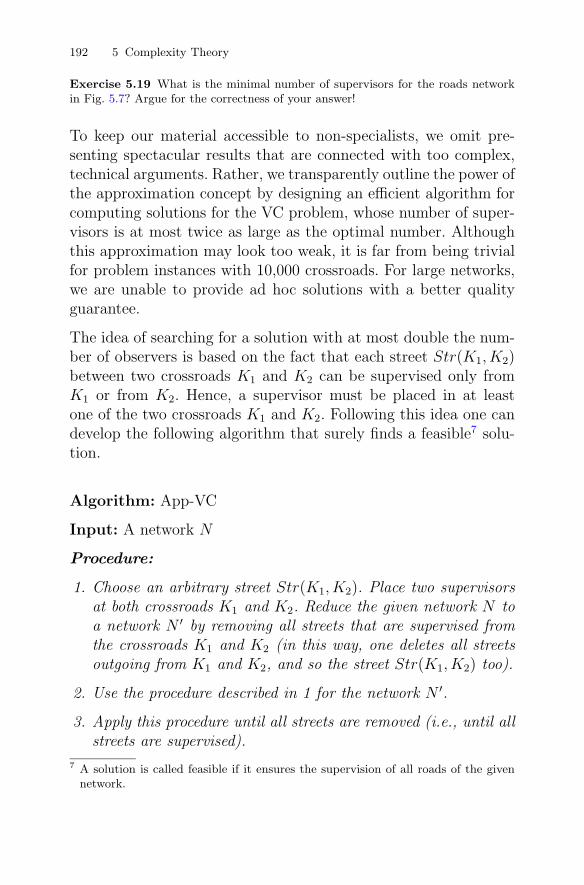
192 5 Complexity Theory
Exercise 5.19 What is the minimal number of supervisors for the roads networkin Fig. 5.7? Argue for the correctness of your answer!
To keep our material accessible to non-specialists, we omit pre-senting spectacular results that are connected with too complex,technical arguments. Rather, we transparently outline the power ofthe approximation concept by designing an efficient algorithm forcomputing solutions for the VC problem, whose number of super-visors is at most twice as large as the optimal number. Althoughthis approximation may look too weak, it is far from being trivialfor problem instances with 10,000 crossroads. For large networks,we are unable to provide ad hoc solutions with a better qualityguarantee.
The idea of searching for a solution with at most double the num-ber of observers is based on the fact that each street Str(K1, K2)between two crossroads K1 and K2 can be supervised only fromK1 or from K2. Hence, a supervisor must be placed in at leastone of the two crossroads K1 and K2. Following this idea one candevelop the following algorithm that surely finds a feasible7 solu-tion.
Algorithm: App-VC
Input: A network N
Procedure:
1. Choose an arbitrary street Str(K1, K2). Place two supervisorsat both crossroads K1 and K2. Reduce the given network N toa network N ′ by removing all streets that are supervised fromthe crossroads K1 and K2 (in this way, one deletes all streetsoutgoing from K1 and K2, and so the street Str(K1, K2) too).
2. Use the procedure described in 1 for the network N ′.
3. Apply this procedure until all streets are removed (i.e., until allstreets are supervised).
7 A solution is called feasible if it ensures the supervision of all roads of the givennetwork.

5.6 Help, I Have a Hard Problem . . . 193
Let us execute the work of algorithm App-VC on the networks inFig. 5.9(a) with 8 crossroads a, b, c, d, e, f, g, and h.
Fig. 5.9
Assume that App-VC chooses the street Str(b, c). This choice isvisualized by the double line in Fig. 5.9(b). Now, two supervisorsare placed at b and c, and all streets outgoing from b and c aredeleted from the network. The deleted streets, except Str(b, c),are marked by the dashed lines in Fig. 5.9(b). Assume the nextchoice of App-VC is the street Str(e, f) (Fig. 5.9(c)). The proce-dure is depicted in Fig. 5.9(c). Two observers are positioned atthe crossroads e and f , and the streets Str(e, f), Str(e, d) andStr(f, d) are marked as supervised. After this, only three streets,Str(d, g), Str(d, h) and Str(h, g), remained unsupervised in thenetwork. If App-VC chooses street Str(d, g), two new supervisorsare placed at the crossroads d and g and the remaining three streetsare supervised. This application of App-VC leads to a solution with6 observers placed at the crossroads b, c, e, f, d, and g.
We observe that the results computed by App-VC may differ andwhat result is computed depends on the random choice of stillunsupervised streets in the first step of the procedure.
Exercise 5.20 How many supervisors does one need in order to supervise the roadnetwork in Fig. 5.9(a)? Find such an unfortunate choice of edges by App-VC that

194 5 Complexity Theory
at the end the supervisors are placed at all 8 crossroads of the network. Does thereexist a random choice of unsupervised edges that results in fewer than 6 supervisors?
Exercise 5.21 Apply the algorithm App-VC in order to place supervisors in net-works in Fig. 5.5 and Fig. 5.7.
Finally, we argue why the solutions produced by App-VC cannotplace more supervisors than twice the optimum. Let us considerthe chosen streets that are marked by double lines in Fig. 5.9.None of these streets meet at a crossroad. This is the consequenceof the fact that, after taking the street Str(K1, K2), all streetsoutgoing from K1 and K2 were deleted for all remaining choices.Hence, no street chosen later can go to K1 and K2. If one takes aglobal look at a network with marked chosen streets (Fig. 5.10),one sees that these are isolated in the sense that no pair of themmeets at a crossroad.
Fig. 5.10
A feasible solution of our VC problem requires that all streets aresupervised. Consequently, all chosen (isolated) streets as a specialsubset of all streets have to be supervised, too. Since the chosenstreets are isolated, one supervisor at a crossroad can supervise atmost one of these streets. Therefore, any feasible solution has atleast as many supervisors as the number of isolated streets. Thesolution of App-VC places supervisors at all end points (cross-roads) of the isolated streets. In this way, the number of observersin the solution computed by App-VC is exactly twice the numberof chosen edges. We see that App-VC cannot compute any solu-tion that would require more than double the optimal number ofsupervisors.

5.7 Summary 195
Certainly, the guaranteed quality of App-VC is not impressive.But there are several complex examples of efficient algorithms forNP-hard problems which compute solutions whose quality doesnot differ from the quality of optimal solutions by more than 1�.Providing the guarantee for such high-quality solutions can beviewed as a miracle of algorithmics.
5.7 Summary
After the notions of algorithms and programs, the notion of com-plexity provides the most fundamental concept of computer sci-ence, and its impact is growing even in scientific disciplines be-yond computer science. Time complexity is the most importantmeasure of computational complexity. It measures the number ofcomputer instructions performed (the amount of computer work).Time complexity is usually represented by a function of the inputsize.
The main goal of complexity theory is classifying algorithmic prob-lems with respect to the amount of work (to the computationalcomplexity) that is sufficient and necessary for computing theircorrect solutions. The final global aim is to define the border be-tween practical solvability and intractability, and so to classify al-gorithmically solvable problems into practically solvable and prac-tically unsolvable. The first approximation of the limit of practicalsolvability proposes that we consider those problems practicallysolvable that can be solved in polynomial-time with respect to theinput length. A problem for whose solution no polynomial-timealgorithm exists is considered to be hard (practically unsolvable).Complexity theory teaches us that there exist problems of an arbi-trarily large complexity. For instance, there exist computing prob-lems that can be solved only by algorithms having time complexityat least 22n
.
To prove the nonexistence of efficient algorithms for solving con-crete computing problems is the hardest research problem in theinvestigation of the laws of information processing. We are not

196 5 Complexity Theory
able to solve this fundamental problem of computer science be-cause we lack sufficiently powerful mathematical methods for thispurpose. Therefore, one currently uses incomplete arguments forarguing about the hardness of some problems. One again uses thereduction method in order to define a large class of equally hardproblems in the sense that each problem of this class can be effi-ciently reduced to any other problem of this class. The consequenceis that either all problems of this class are efficiently solvable ornone of them is efficiently solvable. The problems in this class arecalled NP-hard problems. For none of the NP-hard problems doesone know an efficient polynomial algorithm, and all algorithmsdiscovered for NP-hard problems are of exponential complexity.Because the existence of an efficient algorithm for any of the NP-hard problems would mean the efficient solvability of all NP-hardproblems, and one does not believe in efficient solvability of allthese problems, we consider NP-hardness as a reliable argumentfor the computational hardness of a problem.
The art of algorithm design lies in searching for solutions to hardproblems. The most important discovery is that many hard prob-lems are very unstable with respect to the amount of work nec-essary to solve them (to their hardness). A small (almost negligi-ble8) change of the problem formulation or a small reduction ofthe constraints on feasible solutions may cause an unbelievablyhuge jump from a physically unexecutable amount of computerwork to a matter of a few seconds on a common PC. To discoverand use this sensitivity of hard problems is at the heart of currentalgorithmics [Hro04a], which has the goal of making the solutionof hard problems affordable for industry and, in the end, for thedevelopment of an information society.
Solutions to Some Exercises
Exercise 5.2 Applying the distributive law three times, one can rewrite a polyno-mial of degree 4 as follows:
8 from the practical point of view

5.7 Summary 197
a4 · x4 + a3 · x3 + a2 · x2 + a1 · x + a0
= [a4 · x3 + a3 · x2 + a2 · x1 + a1] · x + a0
= [(a4 · x2 + a3 · x + a2) · x + a1] · x + a0
= [((a4 · x + a3) · x + a2) · x + a1] · x + a0 .
If one applies the resulting formula for computing the value of the polynomial forgiven values of a4, a3, a2, a1, a0, and x, then only 4 multiplications and 4 additionsare performed.
Exercise 5.4
(a) The value of x6 can be computed by 3 multiplications using the following strat-egy:
I ← x · x , J ← I · I , Z ← J · I.
We see the idea starting with computing x2 = x ·x using one multiplication andcontinuing by computing x6 = x2 · x2 · x2 using two multiplications.
(b) The value of x64 can be computed using 6 multiplications as follows:
x64 = (((((x2)2)2)2)2)2
This strategy can be implemented as follows:
I ← x · x , I ← I · I , I ← I · I ,
I ← I · I , I ← I · I , I ← I · I .
(c) One can propose the following strategy for computing the value of x18.
x18 = (((x2)2)2)2 · x2 .
It can be implemented as follows:
I ← x · x , J ← I · I , J ← J · J ,
J ← J · J , Z ← I · J .
(d) The value of x32 can be computed in the following way:
x45 = x32 · x8 · x4 · x= ((((x2)2)2)2)2 · ((x2)2)2 · (x2)2 · x
using the following implementation:
I2 ← x · x , I4 ← I2 · I2 , I8 ← I4 · I4 ,
I16 ← I8 · I8 , I32 ← I16 · I16 , Z ← I32 · I8 ,
Z ← Z · I4 , Z ← Z · x
We see that 8 multiplications are sufficient.
One can even compute the value x45 with 7 multiplications only by using thefollowing strategy:x2 = x · x, x3 = x2 · x, x6 = x3 · x3, x9 = x6 · x3,
x18 = x9 · x9, x36 = x18 · x18, x45 = x36 · x9

198 5 Complexity Theory
Exercise 5.9 If a mathematician has to solve the linear equation a + bx = c + dx,she or he can simplify the equality in the following way:
a + bx = c + dx | − c
a − c + bx = dx | − dx
(a − c) + bx − dx = 0
(a − c) + (b − d) · x = 0 {following the distributive law}
Now, the linear equation has the simplified form, for which we already have analgorithm. In Fig. 5.11 we present the graphic representation of the correspondingefficient reduction.
Fig. 5.11
The reduction R is efficient because two subtractions satisfy in order to transforma general linear equation into the form a′ + b′x = 0. Since a′ + b′x = 0 is only aconversion (another representation) of the equation a + bx = c + dx, both equationshave the same solution. Therefore, the output of the program B is also the outputof the algorithm A for solving general linear equations.
Exercise 5.10 If there is no supervisor at the crossroad K4, there must be 4 super-visors at the other ends of the 4 streets leading from K4 in order to guarantee controlover these four streets. We see that these 4 supervisors supervise the complete roadnetwork (Fig. 5.5).
Exercise 5.17 For the 7 crossroads and at most 3 supervisors one gets first thefollowing linear inequation:
x1 + x2 + x3 + x4 + x5 + x6 + x7 ≤ 3 .

5.7 Summary 199
For 8 streets one gets the following 8 inequalities:
x1 + x5 ≥ 1 , x1 + x6 ≥ 1 , x2 + x5 ≥ 1 , x2 + x6 ≥ 1 ,
x3 + x6 ≥ 1 , x3 + x7 ≥ 1 , x4 + x6 ≥ 1 , x4 + x7 ≥ 1 .
Because of the first inequality, we are allowed to assign the value 1 to at most 3unknowns. The choices x5 = x6 = x7 = 1 and x1 = x2 = x3 = x4 = 0 ensures thatall 8 “street inequations” are satisfied.

Chance favours only those whose spirit has been preparedalready, those unprepared cannot see the hand stretchedout to them by fortune.
Louis Pasteur
Chapter 6
Randomness in Nature and as aSource of Efficiency inAlgorithmics
6.1 Aims
In this chapter we aim to introduce one of the miracles of com-puter science. This marvel is based on a successful applicationof randomness in the design of efficient algorithms for apparentlyintractable problems.
To perform and to understand this magic one has to deal withthe meaning of the notion of “randomness” first. Hence, we fol-low the history of science which is full of controversial discussionsabout the existence of true randomness in order to get a feeling forwhat can be viewed as true randomness and what is only apparentrandomness.
J. Hromkovic, Algorithmic Adventures, DOI 10.1007/978-3-540-85986-4 6,c© Springer-Verlag Berlin Heidelberg 2009
201

202 6 Randomness in Nature
Taking that generated view about randomness we directly moveto algorithmics in order to apply it for solving computationallyhard problems. Here we see a miracle. Can you imagine, at firstglance, that systems with a randomized control can achieve theirgoals billions of times faster than any deterministic system can? Doyou believe that one has to pay for this huge speed-up by riskingmaking an error with probability1 smaller than 1/1019 only? Is thisreally a serious risk? If one had started such a randomized systemevery second since the Big Bang (i.e. between 1018 to 1019 times),then one may have expected none of these many runs to makean error. In another words the probability of making at least oneerror in these more than 1018 experimental runs of this randomizedsystem is smaller than the probability of reaching the correct goalin all these attempts.
Here we call attention to the fact that in practice randomized algo-rithms (algorithms with a random control) with very small errorprobability can be even more reliable than their best determin-istic counterparts. What do we mean by this? Theoretically alldeterministic algorithms may not err. But the nature of the storyis that deterministic programs are not absolutely reliable becauseduring their runs on a computer a hardware error may occur andthen they may produce wrong results. Clearly, the probability ofthe occurrence of a hardware error grows proportionally with therunning time of the program. Therefore a fast randomized algo-rithm can be more reliable than a slow deterministic algorithm. Forinstance, if a randomized algorithm computes a result in 10 sec-onds with an error probability 1/1030, then it is more reliable thana deterministic algorithm that computes the result in one week.Hence, moving from common (deterministic) algorithms and sys-tems to randomized ones is not necessarily related to decreasingreliability. And losing an apparently absolute reliability may nothurt too much. Randomization, here we mean building controllingsystems by using a clever combination of deterministic strategieswith random decisions, became a new paradigm of algorithmics.Efficient randomized algorithms making one mistake in billions of
1 The risk of computing a wrong result is called the error probability.

6.2 Does True Randomness Exist? 203
applications on average are very practical and enable us to solveproblems considered intractable for deterministic computations.
After presenting a magical example to convince ourselves aboutthe power and the usefulness of randomness we do not leave thereader in her or his amazement. We will try to give the reader atleast a feel for why such unbelievably elegant and wonderful waysfor solving problems exist. We get a deeper view into the nature ofthe success of randomized systems and recognize some paradigmsfor the design of randomized algorithms. And, maybe, at the veryend we can even encourage you to use the obtained knowledge inyour everyday life and so to become a magician.
6.2 What Is Randomness and Does There ExistTrue Randomness?
In the first chapter we realized that the creation of notions is fun-damental for the foundation and the development of scientific dis-ciplines. The notion of randomness is one of the few most funda-mental and most discussed notions of science. Philosophers, math-ematicians, physicists, biologists and chemists discussed the exis-tence of randomness and its possible role for thousands of years.Mathematicians created probability theory as an instrument forinvestigating random events. Computer scientists study why andwhen it is profitable to use randomness and design randomizedalgorithms. Engineers apply the obtained knowledge to build effi-cient advantageous randomized systems.
The notion of randomness is strongly related to another two fun-damental notions: determinism and nondeterminism. The de-terministic view of the world is based on the paradigm of causal-ity. Every event has a cause, i.e., every event is a consequenceof a cause. Every cause has its effect (result) and this result is acause of further effects, etc. Following the principle of causality, ifone knows the correct state of the Universe and all natural laws,one can completely predict the future. The whole development is

204 6 Randomness in Nature
viewed as a chain of causes and their effects. By contrast, nondeter-minism means that a cause can have several different consequences(effects) and there is no law determining which one must occur.In another words you can learn all possible results of a cause butonly one of these results may occur and there is no possibility topredict which one.
The notion of randomness is strongly related to nondeterminism.Following the definitions used in dictionaries
an event is considered to be random
if
it happens unpredictably.
Similarly,
an object is called random
if
it is created without any pattern and any plan.
Clearly, the existence of random events (i.e., of the occurrence ofrandomness) contradicts the causality principle. Hence, the follow-ing question
“Does there exist a true (objective) randomness or doesone use this term only to model and describe events withunknown lawfulness?”
is fundamental for science. Philosophers and scientists have dis-puted the answer to this question since ancient times. Democritosbelieved that
randomness is the unknown,and that Nature is determined in its fundamentals.
Thus, Democritos asserted that order conquers the world and thisorder is governed by unambiguous laws. Following Democritos’sopinion, one uses the notion of “randomness” only in the subjec-tive sense in order to veil one’s inability to truly understand the

6.2 Does True Randomness Exist? 205
nature of events and things. Hence the existence of the notion ofrandomness is only a consequence of the incompleteness of ourknowledge. To present his opinion transparently, Democritos likedto use the following example. Two men agreed to send their slavesto bring water at the same time in order to cause the slaves tomeet. The slaves really met at the source and said, “Oh, this israndomness that we have met.”
In contrast to Democritos, Epicurus claimed that
randomness is objective,it is the proper nature of events.
Thus, Epicurus claimed that there exists a true randomness that iscompletely independent of our knowledge. Epicurus’s opinion wasthat there exist processes whose development is ambiguous ratherthan unambiguous, and an unpredictable choice from the existingpossibilities is what we call randomness.
One could simply say, Epicurus was right because there are gamesof chance, such as rolling dice or roulette, that can have differ-ent outcomes, and the results are determined by chance. Unfor-tunately, the story is not so simple, and discussing gambling onegets support for the opinion of Democritos rather than for Epicu-rus’ view on the nature of events. Rolling dice is a very complexactivity, but if one knows the direction, the speed and the sur-face on which a die is tossed, then it may be possible to computeand predict the result. Obviously, the movement of the hand con-trolled by the human brain is too complex to allow us to estimatethe values of all important parameters. But we may not considerthe process of rolling a die as an objectively random process onlybecause it is too complex for us to predict the outcome. The sameis true of roulette and other games of chance. Physics also oftenuses random models to describe and analyze physical processesthat are not inherently or necessarily random (and are sometimesclearly deterministic), but which are too complex to have a real-istic possibility of modelling them in a fully deterministic way. Itis interesting to note that based on this observation even AlbertEinstein accepted the notion of randomness only in relation to an

206 6 Randomness in Nature
incomplete knowledge, and strongly believed in the existence ofclear, deterministic laws for all processes in Nature2.
Before the 20th century, the world view of people was based oncausality and determinism. The reasons for that were, first, reli-gion, which did not accept the existence of randomness in a worldcreated by God3, and, later, the optimism created by the successof natural sciences and mechanical engineering in the 19th century,which gave people hope that everything could be discovered, andeverything discovered could be explained by deterministic causal-ities of cause and resulting effect4.
This belief in determinism also had emotional roots, because peo-ple connected randomness (and even identified it) with chaos,uncertainty, and unpredictability, which were always related tofear; and so the possibility of random events was rejected. Toexpress the strongly negative connotation of randomness in thepast, one can consider the following quotation of Marcus Aure-lius:
There are only two possibilities,either a big chaos conquers the world,or order and law.
Because randomness was undesirable, it may be not surprisingthat philosophers and researchers performed their investigationswithout allowing for the existence of random events in their con-cepts or even tried to prove the nonexistence of randomness byfocusing on deterministic causalities. Randomness was in a sim-ilarly poor situation with Galileo Galilei, who claimed that theEarth is not a fixed center of the whole Universe. Though he wasable to prove his claim using experimental observations, he had nochance to convince people about it because they were very afraid
2 “God does not roll dice” is a famous quotation of Albert Einstein. The equallyfamous reply of Niels Bohr is, “The true God does not allow anybody to prescribewhat He has to do.”
3 Today we know that this strong interpretation is wrong and that the existence oftrue randomness does not contradict the existence of God.
4 Take away the cause, and the effect must cease.

6.2 Does True Randomness Exist? 207
of such a reality. Life in the medieval world was very hard, andso people clung desperately to the very few assurances they had.And the central position of the Earth in the Universe supportedthe belief that poor Man is at the center of God’s attention. Theterrible fear of losing this assurance was the main reason for thesituation, with nobody willing to verify the observations of GalileoGalilei. And “poor” randomness had the same trouble gaining ac-ceptance5.
Finally, scientific discoveries in the 20th century (especially inphysics and biology) returned the world to Epicurus’ view on ran-domness. The mathematical models of evolutionary biology showthat random mutations of DNA have to be considered a crucialinstrument of evolution. But, the essential reason for accepting theexistence of randomness was one of the deepest discoveries in thehistory of science: the theory of quantum mechanics. The mathe-matical model of the behavior of particles is related to ambiguity,which can be described in terms of random events. All importantpredictions of this theory were proved experimentally, and so someevents in the world of particles are considered to be truly randomevents. To accept randomness (or random events) it is very im-portant to overcome the restrictive interpretation of randomness,identifying it with chaos and uncertainty. A very elegant, mod-ern view on randomness is given by the Hungarian mathematicianAlfred Renyi:
Randomness and order do not contradict each other;more or less both may be true at once.Randomness controls the worldand due to this in the world there are order and law,which can be expressed in measures of random eventsthat follow the laws of probability theory.
For us, as computer scientists, it is important to realize that thereis also another reason to deal with randomness beyond the “mere”
5 One does not like to speak about emotions in the so-called exact (hard) sciences,but this is a denial of the fact that the emotions of researchers (the subjects inthe research) are aggregates of development and progress.

208 6 Randomness in Nature
modelling of natural processes. Surprisingly, this reason was for-mulated over 200 years ago by the great German poet JohannWolfgang von Goethe as follows:
The tissue of the worldis built from necessities and randomness;the intellect of men places itself between bothand can control them;it considers the necessityas the reason for its existence;it knows how randomness can bemanaged, controlled, and used...
In this context we may say that Johann Wolfgang von Goethewas the first “computer scientist” who recognized randomness asa useful source for performing certain activities. The use of ran-domness as a resource of an unbelievable, phenomenal efficiency isthe topic of this chapter. We aim to convince the reader that it canbe very profitable to design and implement randomized algorithmsand systems instead of completely deterministic ones. This real-ization is nothing other than the acceptance of Nature as teacher.It seems to be the case that Nature always uses the most efficientand simplest way to achieve its goal, and that randomization ofa part of the control is an essential element of Nature’s strategy.Computer science practice confirms this point of view. In manyeveryday applications, simple randomized systems and algorithmsdo their work efficiently with a high degree of reliability, and wedo not know any deterministic algorithms that would do the samewith a comparable efficiency. We even know of examples where thedesign and use of deterministic counterparts of some randomizedalgorithms is beyond physical limits. This is also the reason whycurrently one does not relate tractability (practical solvability)with the efficiency of deterministic algorithms, but with efficientrandomized algorithms.
To convince the reader of the enormous usefulness of randomiza-tion, the next section presents a randomized protocol that solvesa concrete communication task within communication complex-

6.2 Does True Randomness Exist? 209
ity that is substantially smaller than the complexity of the bestpossible deterministic protocol.
We close this section by calling attention to the fact that we didnot give a final answer to the question of whether or not truerandomness exists, and it is very improbable that science will beable to answer this question in the near future. The reason for thispessimism is that the question about the existence of randomnesslies in the very fundamentals of science, i.e., at the level of ax-ioms, and not at the level of results. And, at the level of axioms(basic assumptions), even the exact sciences like mathematics andphysics do not have any generally valid assertions, but only as-sumptions expressed in the form of axioms. The only reason tobelieve in axioms is that they fully correspond to our experienceand knowledge. As mentioned already in Chapter 1, an exampleof an axiom of mathematics (viewed as a formal language of sci-ence) is assuming that our way of thinking is correct, and so allour formal arguments are reliable. Starting with the axioms, oneconstructs the building of science very carefully, in such a way thatall results achieved are true provided the axioms are valid. If anaxiom is shown to be not generally valid, one has to revise theentire theory built upon it6.
Here, we allow ourselves to believe in the existence of random-ness, and not only because the experience and knowledge ofphysics and evolutionary theory support this belief. For us ascomputer scientists, the main reason to believe in randomnessis that randomness can be a source of efficiency. Randomnessenables us to reach aims incomparably faster, and it would bevery surprising for us if Nature left this great possibility unno-ticed.6 Disproving the general validity of an axiom should not be considered a “tragedy.”
Such events are part of the development of science and they are often responsiblefor the greatest discoveries. The results built upon the old, disproved axiom usuallyneed not be rejected; it is sufficient to relativize their validity, because they aretrue in frameworks where the old axiom is valid.

210 6 Randomness in Nature
6.3 The Abundance of Witnesses Is Support inShortage or Why Randomness Can Be Useful
The aim of this section is to present a task that can be solvedefficiently by applying randomness despite the known fact thatthis task cannot be solved efficiently in any deterministic way. Herewe design a randomized system for solving the mentioned task insuch a simple way that anybody can use it in order to get a firstconvincing experience of the extraordinary power of randomizedcontrol.
What is the exact meaning of a randomized system or random-ized algorithm (program)? In fact one allows two different ba-sic transparent descriptions. Each deterministic program executeson a given input an unambiguously given sequence of computingsteps. We say that the program together with its input unambigu-ously determines a unique computation. A randomized program(system) can have many different computations on the same in-put, and which one is going to be executed is decided at random.In what follows we present two possibilities for the performance ofthe random choice from possible computations.
1. The program works in the deterministic way except for a fewspecial places, in which it may flip a coin. Depending on theresult of coin flipping (head or tail), the program takes one ofthe possible two ways to continue in the work on the input.
To insert this possibility of random choice into our program-ming language TRANSPARENT, it is sufficient to add the fol-lowing instruction:
Flip a coin. If ‘‘head’’, goto i else goto j.
In this way the program continues to work in the i-th row if“head” was the result of flipping coin and it continues in thej-th row if “tail” was the result of flipping coin.
2. The randomized algorithm has at the beginning a choice of sev-eral deterministic strategies. The program randomly choosesone of these strategies and applies it on the given input. The

6.3 Abundant Witnesses Are Useful 211
rest of the computation is completely deterministic. The ran-dom choice is reduced to the first step of computation. For eachnew problem instance the algorithm chooses a new strategy atrandom.
Since the second way of modelling randomized systems is simplerand more transparent than the first one, we use it for the presen-tation of our exemplary application of the power of randomness.
Let us consider the following scenario.
We have two computers RI and RII (Fig. 6.1) that are very farapart. The task is to manage the same database on the computers.At the beginning both have a database with the same content. Inthe meantime the contents of these databases dynamically developin such a way that one tries to perform all changes simultaneouslyon both databases with the aim of getting the same database, withcomplete information about the database subject (for instance,genome sequences), in both locations. After some time, one wantsto check whether this process is successful, i.e., whether RI andRII contain the same data.
We idealize this verification task in the sense of a mathematicalabstraction. We consider the contents of the databases of RI andRII as sequences of bits. Hence, we assume that the computer RI
has a sequencex = x1x2x3 . . . xn−1xn
of n bits and the computer RII has the n-bits sequence
y = y1y2y3 . . . yn−1yn.
The task is to use a communication channel (network) between RI
and RII in order to verify whether x = y (Fig. 6.1).
To solve this task one has to design a communication strategy,called a communication protocol in what follows. The com-plexity of communication and so the complexity of solving theverification problem is measured in the number of bits exchangedbetween RI and RII through the communication channel.

212 6 Randomness in Nature
Fig. 6.1
Unfortunately, the provable fact is that any communication pro-tocol for solving this task cannot do better for most possibleinputs x and y than to exchange n bits. This means that thenaive protocol based on sending all n bits (the whole x) of RI
to RII and asking RII to perform the comparison of x and y bitby bit is optimal. No multiple message exchange and no clevercomputation of RI and RII can help to decrease the commu-nication complexity. If n is very large, for instance n = 1016
(this corresponds to the memory size of 250000 DVDs), thenthe communication cost is too high. Moreover to reliably trans-fer 1016 bits without flipping or losing any particular bit usingcurrent Internet technologies is an almost unrealistic undertak-ing.
In what follows we design a randomized communication protocolthat solves our “equality problem” within
4 · �log2(n)�
communication bits7. We see that one can save an exponentialcomplexity in this way. For instance, for n = 1016 one needs tosend only 256 bits instead of 1016 bits!
For the presentation of the randomized communication strategy itis more transparent to speak about a comparison of two numbersinstead of the comparison of two bit sequences. Therefore we con-sider the sequences x = x1 . . . xn and y = y1 . . . yn of bits as binaryrepresentations of the integers.
7 For a real number a, �a� is the next larger integer. For instance, for a = 4.15,�a� = 5.

6.3 Abundant Witnesses Are Useful 213
Number(x) =n∑
i=1
2n−i · xi
and
Number(y) =n∑
i=1
2n−i · yi
If these formulas do not mean anything to you anymore, and youhave forgotten this secondary-school subject, you do not need toworry about this. The only important thing is to know that
Number(x) is a natural number represented by x, and that
0 ≤ Number(x) ≤ 2n − 1.
Analogously,
0 ≤ Number(y) ≤ 2n − 1.
For n = 1016, these numbers can be really huge. Already for n =106 = 1000000, the numbers can be around
21000000
and consist of about 300000 decimal digits.
Clearly, x and y are identical if and only if Number(x) = Number(y).Hence, we may focus on comparing Number(x) with Number(y)in our randomized protocol.
Exercise 6.1 For those who want to understand everything in detail. The sequence10110 represents the integer
Number(10110) = 1 · 24 + 0 · 23 + 1 · 22 + 1 · 21 + 0 · 20
= 1 · 16 + 0 · 8 + 1 · 4 + 1 · 2 + 0 · 1= 16 + 4 + 2 = 22.
What number is represented by the bit sequence 101001? What is the binary repre-sentation of the integer 133?

214 6 Randomness in Nature
The randomized communication protocol for inputs x1 . . . xn andy1 . . . yn corresponds to a random choice of a collection of determin-istic communication strategies. The size of this collection equalsthe number of primes smaller than n2.
In what follows, for each positive integer m ≥ 2, we denote by
PRIM(m) = {p is a prime | p ≤ m}
the set of all primes in the interval from 1 to m and by
Prim(m) = |PRIM(m)|
the number of primes in PRIM(m).
In what follows we denote by
r = a mod b
the residue of the division a : b. For instance 2 = 14 mod 3, be-cause 14 : 3 = 4 and the remainder is r = 14 − 3 · 4 = 2.
If one considers the division a : b in the framework of integersonly, and the result is c and the remainder is r < b, then one canwrite
a = b · c + r .
In our example for a = 14 and b = 3, the result of the di-vision is c = 4 and the remainder is r = 2. Hence, one canwrite
14 = 3 · 4 + 2,
where r = 2 < 3 = b.
Now, we are ready to present a randomized communication pro-tocol for the comparison of x and y (better to say for comparingNumber(x) with Number (y)).

6.3 Abundant Witnesses Are Useful 215
Randomized communication protocol WITNESS for iden-tity verification.
Initial situation: The computer RI has n bits x =x1x2 . . . xn (i.e., an integer Number(x), 0 ≤Number(x) ≤ 2n − 1).The computer RII has n bits y =y1y2 . . . yn (i.e., an integer Number(y), 0 ≤Number(y) ≤ 2n − 1).
Phase 1: RI chooses a prime p from PRIM(n2) at random. Ev-ery prime from PRIM(n2) has the same probability1/Prim(n2) to be chosen.
Phase 2: RI computes the integer
s = Number(x) mod p
(i.e., the remainder of the division Number(x) : p)and sends the binary representations of
s and p
to RII .
Phase 3: After reading s and p, RII computes the number
q = Number(y) mod p.
If q �= s, then RII outputs “unequal”.If q = s, then RII outputs “equal”.
Before analyzing the communication complexity and the reliabil-ity of WITNESS, let us illustrate the work of the protocol for aconcrete input.
Example 6.1 Let x = 01111 and y = 10110.Hence,
Number(x) = 1 · 23 + 1 · 22 + 1 · 21 + 1 · 20 = 8 + 4 + 2 + 1 = 15,
Number(y) = 1 · 24 + 1 · 22 + 1 · 21 = 16 + 4 + 2 = 22

216 6 Randomness in Nature
and
n = 5.
Consequently n2 = 25 and
PRIM(n2) = {2, 3, 5, 7, 11, 13, 17, 19, 23}.
In Phase 1 the communication protocol WITNESS has the randomchoice from the collection of 9 primes of PRIM(25) and in this wayit chooses one of 9 possible deterministic protocols.
Assume that RI chooses the prime 5. In Phase 2 computer RII
computes
s = 15 mod 5 = 0
and sends the integers p = 5 and s = 0 to RII . Then RII computes
q = 22 mod 5 = 2.
Since 2 = q �= s = 0, the computer RII gives the correct answer
“x and y are unequal”.
Assume now that RI chooses the prime 7 from PRIM(25) at ran-dom. Then the computer RI computes
s = 15 mod 7 = 1
and sends the integers p = 7 and s = 1 to RII . Then RII computes
q = 22 mod 7 = 1.
Since q = s, the computer RII gives the wrong answer
“x and y are equal”.
We immediately observe that WITNESS may err because some ofthe random choices of primes can lead to a wrong answer. �Exercise 6.2 Does there exist a prime in PRIM(23) different from 7, whose choiceresults in a wrong answer of WITNESS for x = 01111 and y = 10110?
Exercise 6.3 Let x = y = 100110 be the inputs. Does there exist a choice of aprime from PRIM(62) such that WITNESS provides the wrong answer “x = y”?

6.3 Abundant Witnesses Are Useful 217
Exercise 6.4 Consider x = 10011011 and y = 01010101 as inputs. Estimate forhow many primes from PRIM(82) WITNESS computes the wrong answer “x = y”.What is the number of primes from PRIM(64) for which WITNESS provides theright answer “x = y”?
First, we analyze the communication complexity of WITNESS.The natural numbers Number(x) and Number(y) have the lengthof their binary representations bounded by n and so they are fromthe interval from 0 to 2n−1. To save communication bits the com-munication of WITNESS consists of sending two integers smallerthan n2, namely p and the remainder of the division Number(x) : p.A natural number smaller than n2 can be binary represented by
⌈log2 n2
⌉≤ 2 · �log2 n�
bits. The symbols � and � are used to denote the rounding tothe next larger integer. For instance, �2.3� = 3, �7.001� = 8 and�9� = 9.
Since in WITNESS two numbers p and s are communicated, RI
can use exactly8 2�log2 n� bits for the representation of each one.In this way the number of communication bits for inputs of lengthn is always exactly
4 · �log2 n� .
Let us see what that means for n = 1016. As already mentioned,the best deterministic protocol cannot avoid the necessity of com-municating at least
1016 bits
for some inputs. Our protocol WITNESS always works within
4 ·⌈log2(1016)
⌉≤ 4 · 16 · �log2 10� = 256 communication bits.
The gap between communicating 1016 bits and 256 bits is huge.Even if it is possible to communicate 1016 bits in a reliable way thecosts of sending 256 bits and of sending 1016 bits are incomparable.For this unbelievably large saving of communication costs we pay
8 If the binary representation of p or s is shorter than 2�log2 n� one can add a few0’s at the beginning of the representation in order to get exactly this length.

218 6 Randomness in Nature
by losing the certainty of always getting the correct result. Thequestion of our main interest now is:
How large is the degree of unreliability we have used to payfor the huge reduction of the communication complexity?
The degree of uncertainty of computing the correct result is calledthe error probability in algorithmics. More precisely, the errorprobability for two input strings x and y is the probability
ErrorWITNESS(x, y)
that WITNESS computes a wrong answer on inputs x and y. Fordifferent input pairs (x, y) (i.e., for different initial situations) theerror probabilities may differ. Our aim is to show that the errorprobability is very small for all9 possible inputs x and y.
“What is the error probability for a given x and y and howcan one estimate it?”
The protocol WITNESS chooses a prime for PRIM(n2) for in-put strings x and y of length n at random. These choices decidewhether the protocol provides the correct answer or not. There-fore we partition the set PRIM(n2) into two parts. All primes thatprovide the correct answer for the input instance (x, y) we call
good for (x, y) .
The prime 5 is good for (01111, 10110) as we have seen in Example6.1.
The other primes whose choices result in the wrong answer for theproblem instance (x, y) we call
bad for (x, y) .
The prime 7 is bad for (01111, 10110) as was shown in Example6.1.9 In computer science we have very high requirements on the reliability of random-
ized algorithms and systems. We force a high probability of getting the correctresult for every particular problem instance. This is in contrast to the so-calledstochastic procedures, for which one only requires that they work correctly withhigh probability on a statistically significant subset of problem instances.

6.3 Abundant Witnesses Are Useful 219
Since each of the Prim(n2) many PRIM(n2) has the same proba-bility of being chosen, we have
ErrorWITNESS(x, y) =the number of bad primes for (x, y)
Prim(n2),
i.e., the error probability is the ratio between the number ofbad primes for (x, y) in the urn (in PRIM(n2)) and the numberPrim(n2) of all primes in the urn. This is a simple considerationand we can convince the reader about it in a transparent way.Assume an urn with 15 balls. Assume that exactly 3 of these 15balls are white. Then the probability of choosing a white ball atrandom is exactly 3
15= 1
5, if each ball has the same probability of
being chosen. In another words, 20% of the balls in the urn arewhite and so one can expect that in a long sequence of repeatedrandom experiments (choosing a ball at random and putting itback) a white ball is the result of the random choice in 20% ofcases. Similarly, flipping a fair coin many times you may expect thenumber of flipped heads is approximately the same as the numberof flipped tails. Analogously, if WITNESS chooses a prime fromthe 15 primes in PRIM(72) for a given (x, y) at random and thereare two bad primes for (x, y) among these 15 primes, the errorprobability for (x, y) is 2/15.
The situation is depicted in Fig. 6.2. Our task is to show, for anyinstance (x, y) of our identity problem, that the set of bad primesfor (x, y) is very small with respect to the size of PRIM(n2).
Fig. 6.2

220 6 Randomness in Nature
How large is PRIM(m) for a positive integer m? One of the deep-est and most important discoveries of mathematics10 is the primenumber theorem saying that
Prim(m) is approximatelym
ln m,
where ln m is the natural logarithm of m. The prime number the-orem says that the primes are closely distributed among natu-ral numbers, because one can find a prime approximately at each(ln m)-th position. For our calculation we need only the knownassertion
Prim(m) >m
ln mfor all integers m > 67. Hence, we have
Prim(n2) >n2
2 ln n
for all n ≥ 9. Our next objective is to show that
for every problem instance (x,y), the number of bad primesfor (x,y) is at most n − 1,
which is essentially smaller than n2/2 ln n.
Investigating the error probability of WITNESS, we distinguishtwo cases with respect to the relation between x and y.
Case 1 x = y and so the right answer is “equal”.
If x = y, then Number(x) =Number(y). For all primes p the equal-ity
s = Number(x) mod p = Number(y) mod p = q
holds. Hence, it does not matter which p from PRIM(n2) is chosen,s = q must hold. In other words, if one divides two equal numbersby the same prime p, the residues of these two divisions mustbe the same. Hence, the protocol WITNESS computes the rightanswer “equal” for all primes in PRIM(n2). Therefore
ErrorWITNESS(x, y) = 0
10more precisely, of number theory

6.3 Abundant Witnesses Are Useful 221
for all strings x = y (for all problem instances (x, y)).
From the analysis of Case 1 we learned that a wrong answer canoccur only for problem instances (x, y) with x �= y.
Case 2 x �= y and so the right answer is “unequal”. As we havealready fixed for (01111, 10110) in Example 6.1, the error prob-ability can be different from 0 for problem instances (x, y) withx �= y. The random choice of p = 7 results in the wrong answer“equal” for x = 01111 and y = 10110.
In what follows we investigate the properties of bad primes for agiven (x, y) in order to prove a general upper bound n − 1 on thenumber of bad primes for every problem instance (x, y) with x �= yand |x| = |y| = n.
A prime p is bad for (x, y) if the residues of the divisions Number(x) :p and Number(y) : p equal each other, i.e., if
s = Number(x) mod p = Number(y) mod p.
The equalitys = Number(x) mod p
means nothing other than
Number(x) = hx · p + s,
where hx is the result of the division Number(x) : p and s < p isthe remainder.
Analogously one can also write
Number(y) = hy · p + s,
where p is involved hy times in Number(y) and s < p is the re-mainder11.
Assume Number(x) ≥Number(y) (in the opposite case whenNumber(y) >Number(x) the analysis can be finished in an anal-ogous way). We compute the integer Number(x)−Number(y) asfollows:11For instance, for x = 10110 we have Number(x) = 22. For p = 5, Number(x) =
22 = 4 · 5 + 2, where hx = 4 and s = 2 is the remainder.

222 6 Randomness in Nature
Number(x)
−Number(y)
Dif(x, y)
hx · p + s
−hy · p − s
hx · p − hy · pIn this way we obtain:
Dif(x, y) = Number(x)− Number(y) = hx ·p−hy ·p = (hx−hy)·p.
The final conclusion is that the prime p divides the number
Dif(x, y) = Number(x) − Number(y).
What did we learn from this calculation?
A prime p is bad for (x, y) if and only if p divides Dif(x, y).
Why is this knowledge helpful? First of all, we have found a fastway of recognizing bad primes.
Example 6.2 Assume RI has the string x = 1001001 and RII hasthe string y = 0101011, both strings of length n = 7. The task isto estimate the bad primes for (x, y) = (1001001, 0101011).
First we estimate
PRIM(n2) = PRIM(49)
= {2, 3, 5, 7, 11, 13, 17, 19, 23, 29, 31, 37, 41, 43, 47}as the set of primes from which WITNESS chooses a primeat random. Following our new observation, the bad primes for(1001001, 0101011) are exactly those primes that divide the differ-ence
Dif(1001001, 0101011) = Number(1001001) − Number(0101011)
= 73 − 43 = 30.
We immediately see that 2, 3, and 5 are the only primes inPRIM(49) that divide 30, and so 2, 3, and 5 are the only badprimes for (1001001, 0101011). In this way we obtain

6.3 Abundant Witnesses Are Useful 223
ErrorWITNESS(1001001, 0101011) =3
Prim(49)=
3
15=
1
5.
�Exercise 6.5 Find all bad primes for the following problem instances.
(i) (01010, 11101)(ii) (110110, 010101)(iii) (11010010, 01101001).
Now, the remaining question is the following one:
“How to use the knowledge that bad primes for (x, y) di-vides Dif(x, y) to bound their number?”
Since both numbers Number(x) and Number(y) are smaller than2n, we have
Dif(x, y) = Number(x) − Number(y) < 2n.
We show that a number smaller than 2n cannot be divisible bymore than n − 1 primes12. To do so we apply another famoustheorem of mathematics, the so-called fundamental theorem ofarithmetics. This theorem says that
each positive integer larger than 1 can be unambiguouslyexpressed as a product of primes.
For instance,
5940 = 2 · 2 · 3 · 3 · 3 · 5 · 11 = 22 · 33 · 5 · 11
and so 2, 3, 5, and 11 are the so-called prime factors of 5940. Inother words, the number 5940 is divisible by exactly 4 primes2, 3, 5, and 11.
Let p1, p2, p3, . . . , pk be all prime factors of our number Dif(x, y)and let p1 < p2 < p3 < . . . < pk. In general, we see that pi > i foreach i. Hence, we have
12Mathematicians would say a number smaller than 2n can have at most n−1 primefactors.

224 6 Randomness in Nature
Dif(x, y) = pi11 · pi2
2 · pi33 · . . . · pik
k
for ij ≥ 1 for all j from 1 to k, and we can write
Dif(x, y) ≥ p1 · p2 · p3 · . . . · pk
> 1 · 2 · 3 · . . . · k= k!
Since Dif(x, y) < 2n and Dif(x, y) > k!, we obtain
2n > k! .
Since n! > 2n for n ≥ 4, k must be smaller than n and in this waywe have obtained the stated aim that
k ≤ n − 1,
i.e., that the number of prime factors of Dif(x, y) is at most n− 1and so the number of bad primes for (x, y) is at most n − 1.
Using this result we can upperbound the error probability of WIT-NESS on (x, y) for x �= y as follows. For every problem instance(x, y) of length n ≥ 9,
ErrorWITNESS(x, y) =the number of bad primes for (x, y)
Prim(n2)
≤ n − 1
n2/ ln n2
≤ 2 ln n
n.
Hence, the error probability of WITNESS for problem instances(x, y) with x �= y is at most 2 ln /n, which is for n = 1016 at most
0.36841
1014.
In Example 6.2 we saw that the error probability can be relativelyhigh, 1/5. This is because the analyzed error probability decreases

6.3 Abundant Witnesses Are Useful 225
with growing n. Therefore, for small problem instances of a fewthousand bits, one recommends to compare x and y in a deter-ministic way, since the costs for such a comparison are anywaysmall. Only for larger problem instances is it profitable to applythe randomized protocol WITNESS.
Exercise 6.6 What are the upper bounds on the error probability of WITNESSfor input sizes n = 103 and n = 104? Up to which problem instance size would yourecommend using the protocol WITNESS?
Exercise 6.7 Estimate the exact error probabilities of WITNESS for the followingproblem instances (x, y):
(i) (00011011, 10101101)(ii) (011000111, 000111111)(iii) (0011101101, 0011110101).
Recently, we have seen a real miracle. A randomized system canefficiently and reliably perform tasks that are not tractable fordeterministic systems. We know many hard problems that can-not be practically solved because the fastest known algorithms forthem require an exponential complexity. Several such problemshave to be solved daily and we are able to perform them only dueto randomized algorithms. The whole area of e-commerce includesimplementations of randomized algorithms in the software used.In fact, bad news for people searching for absolute reliability! But,for those who know the risk and can calculate it and reduce it,randomized systems provide what they are looking for.
Now it is time to at least partially reveal the nature behind themagic of randomization. We want to understand why randomiza-tion can cause such magnificent effects, and thus examine applica-tions of randomization in algorithmics as a natural phenomenon.
We start our considerations by expressing doubts about the successof randomization presented above. We saw that the randomizedprotocol WITNESS works efficiently and with a high reliability.But is it really true that the best deterministic protocol for theidentity problem cannot avoid sending almost n bits for most prob-lem instances, and that for some problem instances the exchangeof n bits is necessary? We did not prove it here. Why may one have

226 6 Randomness in Nature
doubts with respect to these claims? Intuitively, these assertionslook suspicious.
Let us go into detail and look at Fig. 6.2. We rename the goodprimes for (x, y) to witnesses of the difference between x andy (for short).We say that a prime p is a witness of “x �= y” ora witness for (x, y) if
Number(x) mod p �= Number(y) mod p.
A prime q is a non-witness of “x �= y” if
Number(x) mod p = Number(y) mod p.
Thus, the good primes for (x, y) are witnesses for (x, y) and the badprimes are non-witnesses for (x, y). Using these new terms one canview the work of the protocol WITNESS as searching for a witnessof “x �= y”. If WITNESS chooses a witness of “x �= y” at random,then WITNESS proves the fact “x �= y” and reliably provides thecorrect answer “unequal”. If the protocol chooses a non-witnessfor (x, y) with x �= y at random, one cannot avoid the wronganswer “equal”. The protocol WITNESS works correctly with highprobability, because almost all candidates for witnessing inPRIM(n2) are witnesses. The group of non-witnesses is so smallrelative to Prim(n2) that the probability of choosing a non-witnessat random is very small. And now one can present the followingdoubt.
If almost all elements of the set of the candidates for wit-nessing are witnesses for (x, y), why is it not possible to finda witness among them in an efficient, deterministic way andthen to solve the task within a short communication? To fixa witness for (x, y) in a deterministic way means to ex-change the randomness for a deterministic control and soto design an efficient deterministic communication protocolfor the comparison of x and y.
How to explain that this at first glance plausible idea does notwork? Clearly, we can present a formal mathematical proof thatthere is no efficient deterministic communication protocol for this

6.3 Abundant Witnesses Are Useful 227
task. But that is connected with two problems. First, despite thefact that this proof is not too hard for mathematicians and com-puter scientists, it requires knowledge that cannot be presupposedby a general audience. Secondly, understanding of the argumentsof the proof does not necessarily help us to realize why the pro-posed idea does not work. You would only know that designingan efficient deterministic protocol for this task is impossible, butthe main reason for that would remain hidden. Because of that weprefer to present only an idea in a way that increases our under-standing of randomized control.
There is no efficient13 deterministic algorithm for finding a witnessfor a given (x, y), because from the point of view of the computersRI and RII
the witnesses are “randomly” distributed among the candi-dates for witnessing.
What does this mean? If you know x but only very little abouty, you cannot compute a witness for (x, y), even when severalattempts are allowed. This is the consequence of the fact that thewitnesses are completely differently distributed in the candidateset PRIM(n2) for distinct inputs of length n. There is no rule forcomputing a witness for a partially unknown input. Hence, fromthe point of view of RI and RII the soup in the pot containingall candidates (Fig. 6.3) looks as a chaos (a really chaotic mix ofwitnesses and non-witnesses) And this is the kernel of the successof randomness.
For several tasks one can solve the problem efficiently if a witnessis available. In a real application, nobody provides a witness forus for free. But if one can build a set of candidates for witnessingin such a way that this set contains many witnesses, it is naturalto search for witnesses at random. The chaotic distribution of wit-nesses is no obstacle for a random choice. But if the distribution ofwitnesses among candidates is really random, there does not existany efficient deterministic procedure for finding a witness in thisset.13with respect to communication complexity

228 6 Randomness in Nature
Fig. 6.3: A chaotic mix of witnesses and non-witnesses
Searching for efficient randomized algorithms one often applies theidea presented above. We try to find a kind of witness that fulfillsthe following requirements:
(i) If one has a witness for an input instance, then one can computethe correct result efficiently in a deterministic way.
(ii) If one has a candidate for witnessing, one can, for a given input,efficiently verify whether it is a witness or not.
(iii) There is an abundance of witnesses in the set of candidates.
Based on requirement (iii) this method for the design of random-ized algorithms is called the method of the abundance of wit-nesses. Hence, to have many witnesses may be very useful. Howone can even increase the abundance of witnesses is the topic ofthe next section.
6.4 What to Do When a Customer Requires aVery High Reliability?
The whole history of Man is strongly related to the search forcertainty. Who are we? What are we looking for? What to do inorder to get a guarantee for a “nice” or at least any future? Lifeand science educate us that the search for an absolute certainty isa nonsense that can even be dangerous. Striving for a non-existing

6.4 High Reliabilities 229
absolute certainty means to do without many things and activitiesand often means to run up a blind alley. Frustration and depressionare typical consequences of such meaningless effort. But if one ac-cepts uncertainty and with it also randomness as an inevitable partof life and learn to live with this, instead of frustration one discov-ers new possibilities as a reward for giving up non-existing ideals.The blind alleys are not blind anymore and the future is open fora variety of possibilities. That was exactly the case in the examplepresented in the previous section. The situation looked hopeless,because each protocol solving the task has communication coststhat are too large. Exchanging the hypothetical absolute reliabilityof deterministic protocols for a practical reliability of randomizedprotocols, we found a good solution for our communication task.In several similar situations one is unable to find witnesses thathave as high abundance as in our example. Sometimes only a frac-tion of the candidates for witnessing are witnesses. In such casesthe error probability can grow to an extent that is not acceptablein the applications. The aim of this section is to show how one canmaster such situations.
Let us start with our example of the randomized communicationprotocol for the equality of two strings. For n = 1016, the errorprobability is at most 0.37 · 10−14. Assume we have a customer forwhom the reliability of the protocol is extremely important andso he is asking for a still higher degree of guarantee for the correctanswer. For instance, the customer is saying:
“I require the reduction of the error probability to such asmall value, that if one applies the protocol t times for tequal to the product of the age of the Universe in secondsand the number of protons in the Universe, then the proba-bility of getting at least one wrong answer in one of these tapplications is smaller than one in a million.”
For sure, that is a very strange requirement. Can we satisfy thisexaggerated request of the customer without any huge increasein communication complexity? The answer is “YES”, and in or-der to show how to do it we present a simple consideration fromprobability theory.

230 6 Randomness in Nature
Assume we have a fair die. Rolling a die is considered a randomexperiment with 6 possible outcomes 1, 2, 3, 4, 5, and 6, in whichthe probability of each concrete outcome is the same, i.e. 1/6.
Assume that the only “bad” result for us is “1” and all other out-comes of the experiment are welcome. Hence, the probability ofgetting an undesirable outcome is 1/6. Next, we change the exper-iment and the definition of an undesirable outcome. We considerrolling the die five times and the only undesirable outcome of thisnew experiment is to get “1” in all five rolls. In other words, weare satisfied if in at least one of these five simple experiments ofrolling a die the outcome is different from “1”. What is the prob-ability of getting the undesirable outcome? To get the answer,we have to estimate the probability of rolling “1” five times, onebehind another. Because all five die rolls are considered as inde-pendent14 experiments, one calculates as follows. One “1” is rolledwith probability 1/6. Two “1” are rolled one behind another withprobability
1
6· 1
6=
1
36.
The probability of rolling five “1” one behind each other is exactly
1
6· 1
6· 1
6· 1
6· 1
6=
1
65=
1
7776.
What does this consideration have in common with the error prob-ability of randomized communication protocols? A lot. One appli-cation of the randomized protocol can be viewed as a randomexperiment, in which the undesirable outcome corresponds to therandom choice of a non-witness for a given input. Our analysis ofthe error probability of the randomized protocol shows the proba-bility of getting this undesirable outcome, and so the wrong answeris at most
2 ln n
n.
Now, we adapt the idea with the repeated die rolls. If one chooses10 primes at random, then the only undesirable outcome is that all
14The exact meaning of the term independent is presented in [Hro04b].

6.4 High Reliabilities 231
10 primes are non-witnesses for the given input (x, y). If at leastone prime is a witness for (x, y), one gets the correct answer withcertainty. This consideration results in the following randomizedcommunication protocol.
WITNESS (10)Initial situation: Computer RI has n bits x = x1 . . . xn and
computer RII has n bits y = y1 . . . yn.
Phase 1: RI chooses 10 primes
p1, p2 . . . p10 from PRIM(n2) at random.
Phase 2: For each i from 1 to 10 RI computes
si = Number(x) mod pi
and sends the binary representations of
p1, p2 . . . p10, s1, s2 . . . s10
to RII .
Phase 3: After reaching the 20 numbers
p1, p2 . . . p10, s1, s2 . . . s10,
the computer RII computes
qi = Number(y) mod pi
for all i = 1, 2 . . . 10.If there exists at least one i from 1, 2, . . . , 10 such thatqi �= si, then RII knows with certainty that x �= y andoutputs “unequal”.If qi = sj for all 10 j from 1, 2, . . . , 10, then eitherx = y or x �= y and none of the 10 primes chosen is awitness of “x �= y”. In this case the protocol outputs“x = y”.

232 6 Randomness in Nature
What do we observe? If x = y then WITNESS(10) outputs thecorrect result “equal” with certainty, exactly as WITNESS did too.If x �= y, then WITNESS(10) can provide the wrong output onlyif none of the 10 primes chosen is a witness for (x, y). It sufficesthat at least one of these 10 primes is a witness for (x, y), say p4,and RII knows that x �= y because s4 �= p4 and so p4 witnessesthe difference between x and y. If the probability of choosing anon-witness for (x, y) in one attempt is at most 2 ln /n, then theprobability of choosing 10 non-witnesses at random one behindthe other is at most
(2 ln n
n
)10
=210 · (ln n)10
n10.
For n = 1016 this probability is at most
0.4714
10141.
The product of the age of the Universe in seconds and the numberof protons in the Universe is smaller than
1099.
We omit presenting a mathematical calculation that shows thatgetting a wrong output in 1099 applications of WITNESS(10) issmaller than 1 in 1030.
In this way we have reduced the error probability strongly belowany reasonable limits and so we fulfill all reliability requirementsthat have ever been formulated in practice. And we paid very littlefor this wonderful gain. Computing with 10 primes instead of withone increases the communication costs by the multiplicative factor10. Hence, the communication complexity of WITNESS(10) is
40 · �log2n� .
These communication costs are negligible. For instance, for n =1016, WITNESS(10) communicates

6.4 High Reliabilities 233
2560 bits
only.
Since WITNESS(10) can be viewed as 10 repetitions of WITNESS,we say in the formal terms of algorithmics that
the complexity grows linearly with the number of repetitions(attempts to find a witness), while the error probability isreduced with an exponential speed-up in the number of rep-etitions.
In fact, this situation belongs among the most favorable situationsthat one can have when searching for a solution to an algorithmictask.
Our randomized protocol WITNESS(10) is in fact more reliablethan anything we could associate with the notion of reliability.There are two main reasons for that. First, already the proto-col WITNESS provides a high degree of reliability. Secondly, themethod of “repeated experiment” (of repeated random search fora witness) can essentially reduce the error probability even in caseswhen the probability of choosing a witness at random is small. Thefollowing exercises provide the reader with the possibility of ap-plying the ideas presented above and so deepen one’s imaginationof the power of randomized computation.
Exercise 6.8 Let A be an algorithmic task for which every known algorithm hascomplexity at least 2n. Let A be a decision problem for which only answers YESand NO are possible and so the task is to decide whether a problem instance x hasa special property or not. Assume one has a kind of witness for x of size n with thefollowing properties:
(i) If z is a witness for x, then one can verify in 10 · n2 operations that x has thedesired property. If z is not a witness for x, then the algorithm is unable torecognize whether x has the desired property or not. The fact that z is not awitness for x is recognized by the algorithm in time 10 · n2, too.
(ii) At least half of the witness candidates are witnesses, i.e. the probability ofchoosing a witness at random is at least 1/2.
The tasks are as follows:
1. Assume a randomized algorithm that performs 10 choices from the set of witnesscandidates at random in order to get a witness for the given input. Bound theerror probability of this algorithm and analyze its computational complexity.

234 6 Randomness in Nature
2. A customer is asking for an algorithm that solves the decision problem with errorprobability at most 1 in 109. How many repetitions of the original algorithmare necessary to reduce the error probability below this limit? What is thecomplexity of the resulting algorithm?
Exercise 6.9 Solve Exercise 6.8 if the assumption (i) is satisfied, and instead of(ii) we have the following assumptions:
(i) The portion of witnesses in the set of candidates is exactly 1/6.(ii) The portion of witnesses in the set of candidates is only 1 in n, where n is the
size of the problem instance (input).
6.5 What Are Our Main Discoveries Here?
If, for some tasks, one strongly requires to compute the correctresults with absolute certainty, one can walk up a dead-end street.All algorithms that assume a theoretically absolute reliability de-mand so much computer work that they are intractable (not prac-ticable). We know several computing tasks for which the bestknown algorithms need more time than the age of the Universeand more energy than the energy of the whole known Universe.To solve such problems is beyond the limits of physically doable.And then we discover that there is a magic way to solve these hardtasks. We do without the absolute reliability that does not existanyway in practice and force a high probability of computing thecorrect result for each problem instance instead. We are allowed torequire such a small error probability that one can speak about ex-changing a hypothetical absolute reliability for practical certaintyof getting the right result. Due to this fictitious reduction of ourreliability requirements, we can save a huge amount of computerwork. There exist problems for which a clever use of randomnesscauses a big jump from a physically undoable amount of work toa few seconds work on a common PC.
We learned two important paradigms for the design of randomizedsystems. The method of abundance of witnesses touches upon thedeepest roots of the computational power of randomness. A wit-ness for a problem instance is a piece of additional information

6.5 What Are Our Main Discoveries Here? 235
that helps us to efficiently solve the problem instance that cannotbe solved efficiently without it. The method promises successfulapplications if one can find a kind of witness, such that there isan abundance of witnesses in the set of candidates for witnessing.The idea is then to use repeated random sampling (choice) fromthe set of candidates in order to get a witness efficiently with highprobability, although one does not know any efficient way of com-puting a witness using deterministic algorithms. The question ofwhether there are problems that can be solved efficiently by ap-plying randomization, but which cannot be solved efficiently in adeterministic way, can be expressed as follows:
If all kinds of sets of candidates for witnessing for a hardproblem have the witnesses randomly distributed in the can-didate set then the problem is efficiently solvable using arandomized algorithm, but not efficiently solvable using de-terministic algorithms.
The second approach we applied for the design of randomized al-gorithms is the paradigm of increasing success probability (of a fastreduction of error probability) by repeating several random compu-tations on the same problem instance. This paradigm is often calledthe paradigm of amplification (of the success probability). Repeat-ing WITNESS 10 times results in the protocol WITNESS(10),whose error probability tends to 0 with an exponential speed inthe number of repetitions, but whose complexity grows only lin-early in the number of repetitions. The situation is not alwaysso favorable, but usually we are able to satisfy the reliability re-quirements of customers without paying too much with additionalcomputer work.
The textbook “The Design and Analysis of Randomized Algo-rithms” [Hro04b, Hro05] provides a transparent introduction tomethods for designing efficient randomized systems. On one side itbuilds the intuition for the subject in small steps, and on the otherside it consistently uses the rigorous language of mathematics inorder to provide complete argumentation for all claims related tothe quality of designed algorithms in terms of efficiency and error

236 6 Randomness in Nature
probability. The most exhaustive presentation of this topic is avail-able in Motwani and Raghavan [MR95]. But this book is writtenfor specialists and so it is not easily read by beginners. A delicacyfor gourmets is the story about designing algorithms for primal-ity testing by Dietzfelbinger [Die04], where the method of abun-dance of witnesses is applied several times. Further applicationsfor designing randomized communication protocols are availablein [KN97, Hro97]. Here, the mathematically provable advantagesof randomness over determinism are presented. Unfortunately, be-cause many highly nontrivial mathematical arguments are consid-ered, these books are not accessible to a broad audience.
Solutions to Some Exercises
Exercise 6.2 The prime 7 is the only prime in PRIM(25) whose choice in the firststep of WITNESS results in a wrong output “equal” for the input x = 01111 andy = 10010.
Exercise 6.5 (i) Let x = 01010 and y = 11101. Hence, n = 5 and we considerprimes from PRIM(52). The integers represented by x and y are:
Number(01010) = 23 + 21 = 8 + 2 = 10
Number(11101) = 24 + 23 + 22 + 20 = 16 + 8 + 4 + 1 = 29.
To find the bad primes from PRIM(25) for x and y, we do not need to test all primesfrom PRIM(25). We know that every bad prime for x and y divides the difference
Number(11101) − Number(01010) = 29 − 10 = 19
The number 19 is a prime and so 19 is the only prime in PRIM(25) that 19 divides.Hence, 19 is the only bad prime for 01010 and 11101.
Exercise 6.7 (i) To calculate the error probability of WITNESS for x = 00011011and y = 10101101, we need to estimate the cardinality of PRIM(82).
PRIM(64) = {2, 3, 5, 7, 11, 13, 17, 19, 23, 29, 31, 37, 41, 43, 47, 53, 59, 61}
and so |PRIM(64)| = 18. The integers represented by x and y are:
Number(x) = 24 + 23 + 21 + 20 = 16 + 8 + 2 + 1 = 27
Number(y) = 27 + 25 + 23 + 22 + 20 = 128 + 32 + 8 + 4 + 1 = 173.
Hence, Number(y)−Number(x) = 173− 27 = 146. The factorization of the number146 is:
146 = 2 · 73 .
Thus, the integers 2 and 73 are the only primes that divide the difference

6.5 What Are Our Main Discoveries Here? 237
Number(y) − Number(x) .
The prime 73 does not belong to PRIM(64) and so the prime 2 is the only bad primefor (x, y) in PRIM(64). Hence, the error probability of the protocol WITNESS for(01010, 11101) is exactly 1/18.
Exercise 6.8 The algorithm halts when it finds a witness for x. In the worst case, thealgorithm performs 10 attempts and each attempt costs at most 10·n2 operations forchecking whether the chosen candidate is a witness for x. Therefore the worst-casecomplexity of the randomized algorithm is 20·10·n2. If the input x does not have theproperty we are searching for, the algorithm provides the right answer “NO” withcertainty. If x has the property, then the algorithm can output the wrong answer“NO” only when it chooses 20 times a non-witness for x. We assume (assumption(ii) of the exercise) that the probability of choosing a non-witness at random in anattempt is at most 1/2. Hence, the probability of choosing no witness in 20 attemptsis at most
„
1
2
«20
=1
220=
1
1048576≤ 0.000001 .
In this way we determined that the error probability is smaller than 1 in one million.
How many attempts are sufficient in order to reduce the error probability below1/109? We know that 210 = 1024 > 1000. Hence,
230 = (210)3 > 10003 = 109 .
Thus, 30 attempts suffices for getting an error probability below 1 in one million.

From a genius idea all words can be removed.
Stanis�law Jerzy Lec
Chapter 7
Cryptography, or How toTransform Drawbacks intoAdvantages
7.1 A Magical Science of the Present Time
In the 20th century physics was probably the most fascinatingscience. It brought discoveries that have essentially changed ourview on the world. Many interpretations and applications of thetheory of relativity or of quantum mechanics look like miracles.Things and events considered to be impossible became fundamen-tal for building physical theories. We consider cryptography to bea magical science of the present time that transfers knowledge intomagic. Do you believe that
• one can convince everybody about having a secret without re-vealing any small fraction of the secret?
J. Hromkovic, Algorithmic Adventures, DOI 10.1007/978-3-540-85986-4 7,c© Springer-Verlag Berlin Heidelberg 2009
239

240 7 Cryptography
• one can send a message in cipher to several receivers in such away that they can read it only if all receivers cooperate (i.e.,they put their secrets together)?
• one can sign a document electronically in such a way that ev-erybody is convinced about the authenticity of the signaturebut nobody can fake (emulate) it?
• one can agree on a common secret with another person in apublic talk in such a way that no listener gets any informationabout the secret?
That and still much more is possible. Pure magic.
Communication is the generic term of the current era. It does notmatter whether one uses mobile phones, SMS, e-mail or classicalfax, phones or letters. Communication is present at every timeand everywhere. A large amount of data is permanently flowingvia the Internet. With the amount of data submitted, the difficultyof ensuring the privacy of all parties involved in communicationincreases. This is not only the problem of ensuring that only theproper receiver is able to read a message submitted to him. In thecase of online banking, e-commerce or e-voting, the requirementson the degree of security grow enormously.
Cryptology is the science of secret writing and is almost as old aswriting itself. In cryptology, we distinguish between cryptogra-phy and cryptanalysis. Cryptography is devoted to the design ofcryptosystems (secret codes), while cryptanalysis is devoted to theart of attacking cryptosystems (illegally intercepting messages). Atthe beginning, when writing was discovered, very few people wereable to read or to write. Hence, at that time writing was consideredto be secret in the sense that the ability to read was a commonsecret of a small group of insiders. The need for special secretwriting grew with the growing number of people who were ableto read. Here we start with providing some impressions about thetime when secret writing was an art. One developed a secret codeand used it until somebody deciphered it and so made its use inse-cure. In that time, cryptology was a game between two intellects,

7.2 Prehistory of Cryptography 241
namely the secret code designer and a secret code hacker. First,we will have a look at encryptions used by Caesar and Richelieu.In this way, we get the first impression of what cryptosystems areand what the security of cryptosystems means.
Our next aim is to show that, due to computer science, especiallydue to algorithmics and complexity theory, the art of designingcryptosystems has become a science called cryptography. Cryptog-raphy owes a debt to algorithmics for the definition of the notion ofthe security of cryptosystems. The algorithmic concept of securitybecame the axiomatic base for scientific investigation. Using it, onedeveloped modern cryptography, which is based on the mystery ofso-called public-key cryptosystems. Here, we explain the idea be-hind this mystery that transfers our drawbacks and inability tosolve some problems into advantages. The existence of efficientlyunsolvable algorithmic problems (which was discussed in Chapter5) is used to make algorithmic cracking of designed cryptosystemsimpossible. Finally, we present some miracles that can be viewed as“magic” applications of the concept of public-key cryptosystems.
7.2 The Concept of Cryptosystems or a FewImpressions from the Prehistory ofCryptography
First, we fix our terminology. As already mentioned above, weconsider cryptology as teachings of secret writing. We distinguishbetween cryptography and cryptanalysis. Cryptography is the sci-ence of designing secret cryptosystems. Cryptanalysis is devotedto attacking them. Here, we deal with cryptography only. The sce-nario we consider is presented in Fig. 7.1.
A person, called the sender, aims to send a secret message toanother person, called the receiver. The secret message can berepresented as a text, called a plaintext. The plaintext can bewritten in a natural language, and therefore it is readable for ev-erybody. There is no other possibility besides communicating the

242 7 Cryptography
Fig. 7.1
secret through a publicly accessible network, where one cannotexclude the possibility that other persons can “listen” to the com-munication messages transported in the network. To exclude thepossibility that an unauthorized person listening to the messagelearns about the secret, one sends the message in an encryptedform using a secret writing. The kind of encryption and of de-cryption is a common secret of the sender and of the receiver, andthe encryption is performed using the so-called key. The encryptedtext is called the cryptotext. The cryptotext is sent via the pub-lic network. Upon receiving the cryptotext, the receiver decryptsthe cryptotext and obtains the original plaintext. A description ofthe processes of encrypting and decrypting the messages providesfull information sufficient for using the cryptosystem.
To illustrate it using a transparent example, we present the cryp-tosystem CAESAR that was really used by Caesar. The plaintextwere texts over the Latin alphabets. The special symbols such asblank, comma, period, and question mark were omitted. In thisway the text
VENIVIDIVICI
can be viewed as a plaintext. Caesar encoded each letter unam-biguously by another letter. The keys are the integers
0, 1, 2, 3, 4, 5, . . ., 23, 24, 25.
To apply a key i means that every symbol of the plaintext is re-placed by the letter that is k steps (positions) to the right in thealphabetical order. If the end of the alphabet is reached, one con-tinues cyclically from the beginning.

7.2 Prehistory of Cryptography 243
Figure 7.2 shows the encoding using the key i = 3. This meansthat A in the plaintext is represented by D in the cryptotext,because A is at the first position of the Latin alphabet and, shiftingby 3 positions, one reaches the fourth position occupied by D.Analogously, the letter B at the second position is replaced by theletter E at the fifth position, etc. In this way, the letter W at the23rd position is replaced by the letter Z at the 26th position. Howto encode the last three letters X, Y, and Z at the positions 24, 25,and 26, respectively? One still did not use the letters A, B, and Cin the cryptotext. We simply write the letters A, B, and C at thepositions 27, 28, and 29 behind our alphabet, as depicted in Fig.7.2. In this way, our problem of replacing X, Y, and Z is solved.The letter X is replaced by A; Y is replaced by B; Z is replacedby C. Another transparent way of describing the cryptosystemCAESAR is to write the Latin alphabet on a tape and then stickthe ends of the tape together (Fig. 7.3). Now, rotating the tapeby 3 positions, one gets the codes of the letters. Applying the keyi = 3 for the plaintext VENIVIDIVICI, one gets the cryptotext
YHQLYLGLYLFL .
Fig. 7.2
Fig. 7.3

244 7 Cryptography
Exercise 7.1 (a) Encode the plaintext VENIVIDIVICI using the key i = 5 andthen using the key i = 17 using the cryptosystem CAESAR.(b) Encode the plaintext “Roma aeterna docet” using the key i = 7, and the plain-text “Homines sumus, non dei!” using the key i = 13.
How does the receiver decode the cryptotext? She or he simply re-places each letter of the cryptotext by the letter that is 3 positionsbefore this letter in the alphabet. It corresponds to twisting thetape in Fig. 7.3 three positions to the left. In this way, for instance,the letter S of the cryptotext is replaced by P, U is replaced for R,and L is replaced by I. Hence, one decrypts the cryptotext
SULPXPQHQRFHDV
encrypted using the key i = 3 and obtains the original plaintext
PRIMUMNENOCEAS .
Exercise 7.2 Decrypt the cryptotext WYPTBTBAWYVMPJLHZ encrypted usingthe key i = 7.
To be more precise, Caesar tried to decrease the risk that some-body could look through his cryptosystems and therefore he madeit more complicated. After shifting the letters, he replaced the let-ters of the Latin alphabet one by one using the letters of the Greekalphabet. Hence, the receiver had to replace the Greek letters forthe Latin ones first, and then to shift positions back inside of theLatin alphabet.
Jules Verne discussed in his novels a cryptosystem generalizingthat of Caesar. Any integer was allowed to be a key. For an integerof m digits
A = a1a2 . . . am
he partitioned the plaintext into blocks of length m and replacedthe jth letter of each block by the letter that was aj positions afterthe letter in an alphabetical order. For instance, for a = 316 onegets for the plaintext
C R Y P T O G R A P H Y
3 1 6 3 1 6 3 1 6 3 1 6
the cryptotext
FSESUUJSGSIE .

7.2 Prehistory of Cryptography 245
Fig. 7.4
In contrast to the factual cryptosystem CAESAR, Richelieu culti-vated in his cryptosystem a real literary art. The following exampleis due to Arto Salomaa [Sal96]. The cryptotext is a well-structuredletter on a sheet. Each letter has an exact position on the sheet.For instance, H lies at the intersection of the second row and ofthe third column in Fig. 7.4(b). The key is the matrix in Fig.7.4(a) that covers some fields of the sheet (the grey ones in Fig.7.4(b)) and leaves some fields open for reading. The uncoveredletters build the plaintext (Fig. 7.4(c)). For the friendly lookingcryptotext in Fig. 7.4(a), the plaintext is
YOUKILLATONCE .

246 7 Cryptography
7.3 When Is a Cryptosystem Secure?
People have always strived for security and certainty. The unknownand uncertainty are often the main reasons for fear. In spite of this,science, and especially physics, teaches us that absolute certaintydoes not exist. To strive for it can even result in an illness. It isbetter to learn to live with uncertainty. Anyway, it may be rea-sonable to strive for an achievable degree of security. When is oneallowed to consider a cryptosystem to be secure? Always when anadversary of an unauthorized person is unable to get the plaintextfrom the cryptotext sent. This requirement allows two differentinterpretations. Does one require it to be hard or even impossibleto decrypt a cryptotext if nothing about the used cryptosystem isknown or if the cryptosystem (the kind of encryption) is knownand only the key is secret? The first option with the whole cryp-tosystem as a secret is called “security by obscurity”, and one doesnot consider it to be a reasonable base for defining the security ofcryptosystems. This is because experience shows that revealingthe kind of encryption of a new cryptosystem is only a question oftime.
Therefore, already in the 19th century Auguste Kerckhoffs pre-sented the following requirement on the security of cryptosystems,known as Kerckhoffs’ principle:
A cryptosystem is secure, if one, knowing the art of thefunctioning of the cryptosystem but not knowing the keyused, is not able to derive the original plaintext from thegiven cryptotext.
We immediately see that under this definition of security the cryp-tosystem CAESAR is not secure. If one knows the principle ofCAESAR, it suffices to try out all 26 keys in order to decrypt anycryptotext.
A direct consequence is that secure systems have to have a hugenumber of keys. By “huge” we mean that even the fastest com-puters are unable to try out all of them. The next question is,whether a large number of possible keys guarantees the security of

7.3 When Is a Cryptosystem Secure? 247
a cryptosystem. Consider an improvement of CAESAR by allow-ing arbitrary pairs of letters. Then keys are defined by the so-calledpermutations of 26 letters that can be viewed as 26-tuples of in-tegers between 1 and 26. In any 26-tuple, each integer from theinterval 1 to 26 occurs exactly once. For instance, the key
(26, 5, 1, 2, 3, 4, 25, 24, 23, 8, 9, 22, 21, 20, 7, 6, 10, 11, 18,17, 12, 13, 19, 14, 16, 15)
corresponds to the following encryption. The first letter A is re-placed by the 26th letter Z, the second letter B is replaced by thefifth letter E, the third letter C is replaced by the first letter A,etc. The complete description of the resulting pairing of letters isgiven in Fig. 7.5.
Fig. 7.5
Applying this key, one gets the cryptotext
QXCKCWRTBYKCZQCKBZUZYCQXZTQXCQWUCVGRQ
for the plaintext
THEREISNOGREATERDAMAGETHANTHETIMELOST.
Exercise 7.3 Decrypt the following cryptotexts that were encrypted using the keydescribed in Fig. 7.5.
(a) AKPFQGYKZFXP(b) RCALKC
How many keys are possible in this cryptosystem? To code A onehas the choice from 26 letters of the Latin alphabet. After choosinga letter decoding A, one has 25 possibilities to choose a letter cod-

248 7 Cryptography
ing B. For C, one has still 24 possibilities, etc. Hence, the numberof all keys is
26! = 26 · 25 · 24 · 23 · . . . · 3 · 2 · 1.
In the language of combinations, one says that 26! is the numberof all permutations of 26 elements. This number is huge, approxi-mately equal to 4.03 · 1026. No computer is fast enough to be ableto try out so many keys.
Does it mean that this system is secure? Unfortunately, “No” isthe unambiguous answer. To discover the key applied, one does notneed to try out all possibilities. A clever idea (that did not occur tothe cryptosystem designer) suffices to crack this cryptosystem. Inthe case of our cryptosystem based on permutations of letters, it issufficient to know which natural language is used for the plaintext.For each natural language, one knows the statistical frequency ofthe occurrence of particular letters, and these frequencies can differa lot from letter to letter. Additionally, some letter combinationssuch as TH in English and SCH in German are very frequent. Anexperienced cryptanalyst can use this knowledge to estimate thekey (the letter permutation) and so to decrypt the cryptotext ina few minutes.
This example shows the enormous difficulty of measuring the de-gree of security (reliability) of a given cryptosystem. What doesit mean that it is impossible or hard to crack a cryptosystem?The problem with the definition of security by Kerckhoffs is thatone more dimension is involved there. Besides the cryptosystem it-self, there is an adversary in the game. What is impossible for oneadversary does not need to be hard for another, genius one. An ex-cellent idea may reduce the decryption problem to an easy game.What is one allowed to assume about the facilities of an adversary,or how to get all cryptanalysts under one uniform description?
Computer science solved this long-standing open problem of mak-ing the definition of secure cryptosystems clear enough. It coveredall simple as well as in ingenious strategies of cryptanalysts usingthe notion of an algorithm.

7.4 Symmetric Cryptosystems 249
A cryptosystem is secure if there does not exist any efficient(randomized polynomial) algorithm that decrypts cryptotextwithout knowing the secret key used, but knowing the wayin which the cryptosystem works.
Clearly, this definition of secure cryptosystems could not be dis-covered before the notion of algorithm and the concept of compu-tational complexity were introduced. Due to them, one was ableto exactly formulate the first two fundamental requirements ona “good” cryptosystem in the scientific terminology provided bycomplexity theory.
(i) Encryption and decryption can be efficiently performed by al-gorithms when the key is known.
(ii) Decryption without knowledge of the secret key used in en-crypting the plaintext corresponds to a hard (practically un-solvable) problem.
7.4 Symmetric Cryptosystems
The cryptosystems presented until now are called symmetric.The term symmetric points to the fact that the sender and thereceiver are equal in the sense that the same key as a commonsecret is used to encrypt as well as to decrypt the messages. Infact, the sender and the receiver can exchange their rules anytime,and so the communication can be viewed as gossiping or as aninformation exchange.
In what follows, we show a secure symmetric communication sys-tem. For this cryptosystem we assume that the plaintexts are sim-ply sequences of zeros and ones. This is not a restriction becauseeach letter of an alphabet as well as each symbol of the keyboardhas an ASCII code that is the binary representation of the cor-responding letter used in computers. In this way, one can firsttransform any text into a sequence of zeros and ones.
One also uses as keys sequences of zeros and ones. These sequenceshave to be long, for instance a few hundred bits, in order to get

250 7 Cryptography
many keys. They have to be generated at random in order to maketheir computation impossible for each unauthorized person.
To describe encryption and decryption (i.e., to define the cryp-tosystem), we have first to introduce a special operation on bits(binary numbers). This operation is called “exclusive or” or “XOR”and is denoted by ⊕. It is defined as follows:
0 ⊕ 0 = 0 1 ⊕ 1 = 0 0 ⊕ 1 = 1 1 ⊕ 0 = 1
Following the notation from Chapter 6, one can write a ⊕ b =a + b mod 2. If a and b are equal, the result is 0. If a and b aredifferent, the result is 1.
Assume that the key is 01001011. The length of the key is 8 andthe key can be applied to encrypt plaintexts of length 8. The ithbit of the key is used to encode the ith bit of the plaintext. Onecan see the encryption transparently if one writes the key belowthe plaintext as follows:
plaintext 00001111
⊕ key 01001011
= cryptotext 01000100
The ith bit of the cryptotext is the XOR-sum of the ith bit of theplaintext and the ith bit of the key. Interestingly, one can use thesame procedure for decryption:
cryptotext 01000100
⊕ key 01001011
= plaintext 00001111
We see that it works and that the original plaintext was decrypted.The success of this procedure is based on the fact that
a ⊕ a = 0, and so b ⊕ a ⊕ a = b.
Hence, two applications of the same key result in the original text.In another words, the second application of the key deletes thefirst application. Moreover,

7.4 Symmetric Cryptosystems 251
a ⊕ b = b ⊕ a
holds, and therefore we call this cryptosystem commutative.
Exercise 7.4 Encode and decrypt the plaintext 0001110011 using the key 0101101001.
Exercise 7.5 Build a similar cryptosystem that is based on the operation ⊥ definedas follows:
0 ⊥ 0 = 1 1 ⊥ 0 = 0 1 ⊥ 1 = 1 0 ⊥ 1 = 0
The second bit b in a ⊥ b is called a mask. If b = 1, then the first bit a is copied. Ifb = 0, then the first bit a flips to a (i.e., 1 flips to 1 = 0 and 0 flips to 0 = 1).
(a) Apply the operation ⊥ instead of ⊕ in order to encrypt and then decrypt theplaintext 00110011 using the key 00101101.
(b) Explain why the cryptosystem based on ⊥ also works and has the same prop-erties as the cryptosystem based on ⊕.
(c) What have the operations ⊥ and ⊕ in common? Does there exist a strongrelationship between them?
If the key is generated together by the sender and the receiver1
at random and then applied in order to mask, one can prove us-ing mathematical instruments that the cryptotext is viewed asa random sequence of bits to any third party. In this case, nocryptoanalyst has a chance to decrypt the message because no al-gorithm, even ones with exponential complexity, can help. For asingle application, this system is considered to be absolutely se-cure.
If one has a long plaintext and a key of a fixed length n, the usualway of encrypting the text is based on partitioning the text into asequence of slices of length n and then applying the key separatelyto each slice. For instance, one can use the key 0101 to encryptthe plaintext
1111001100001101
as follows. One cuts the plaintext into four slices 1111, 0011, 0000,and 1101 and applies the key 0101 to each slice separately. Afterconcatenating the resulting slices, one gets the cryptotext
10100110010110001 That is, the key does not need to be communicated by a public link.

252 7 Cryptography
that is sent to the receiver. This is the typical way in which cryp-tosystems based on a fixed key work for arbitrarily long mes-sages.
In the case of an XOR-cryptosystem, one does not recommend thisextension for messages of any arbitrary length, because multipleapplications of the same key on several slices can help to calculatethe key. Moreover, the fact
plaintext ⊕ cryptotext = key (7.1)
holds. Let us check this property for the key 01001011 used in ourexample above:
plaintext 00001111
⊕ cryptotext 01000100
= key 01001011
Why is this true?
plaintext ⊕ key = cryptotext (7.2)
is our encryption method. Now, we add the plaintext to both sidesof Equality (7.2) from the left and obtain the following equality:
plaintext ⊕ plaintext ⊕ key = plaintext ⊕ cryptotext (7.3)
Since a ⊕ a = 0 for each bit a,
plaintext ⊕ plaintext = 00 . . . 00 .
Since 0 ⊕ b = b for each bit b, the left side of Equality (7.3) is thekey, and hence we obtain Equality (7.1).
The validity of Equality (7.1) can be very dangerous for the secu-rity of a cryptosystem. If by a multiple use of a key the adversaryobtains only one pair (plaintext, cryptotext) in some way, then byapplying (7.1) she or he can immediately calculate the key and sodecrypt all other cryptotexts. Therefore, the XOR-cryptosystemis secure for a single application only.

7.5 How to Agree on a Secret in Public Gossip? 253
Exercise 7.6 (challenge) Try to design a secure cryptosystem for the followingapplication. A person A encrypts a plaintext (a confidential message) using a secretkey that nobody else knows. The confidential message is sent as the cryptotext totwo persons B and C. Now, A wants to distribute the secret key to B and C in sucha way that neither B nor C alone is able to decrypt any single bit of the message,but B and C cooperating together can calculate the plaintext without any problem.
There are symmetric cryptosystems that are considered to be se-cure, and one is allowed to use the same key many times withoutworry. The famous and most frequently used symmetric cryptosys-tem is DES (Data Encryption Standard) developed in a cooper-ation between IBM and NSA (National Security Agency). DESalso uses the XOR-operation several times, but this cryptosystemis too complex to be described here.
In spite of the high reliability of some symmetric cryptosystems,we are still not finished with trip devoted to searching for a securecryptosystem. The main drawback of symmetric cryptosystems isthat they can be successfully applied only if the sender and thereceiver agree on a common secret key before the cryptosystem isapplied. But how can they do this without any personal meeting?How can they agree on a secret key without any secure cryptosys-tem when they are restricted to communication via a public, in-secure channel? How to solve this problem is the topic of the nextchapter.
7.5 How to Agree on a Secret in Public Gossip?
Two persons, Alice and Bob, want to create a common cryptosys-tem. The encryption and the decryption procedures are known toboth, and they only need to agree on a common secret key. Theydo not have the opportunity to meet each other and are forced toagree on (to generate) a common secret using a public, insecurechannel without applying any cryptosystem. Is this possible?
The answer is “Yes”, and the elegant solution is a real surprise.First, we introduce the idea of using a chest with two locks and anuntrustworthy messenger. Alice has a private lock with a unique

254 7 Cryptography
key and so nobody else can close and unlock her lock. Similarly,Bob has his private lock with a unique key. They do not haveany common key. Alice and Bob agree publicly that Alice is goingto send Bob a future common key in the chest. They proceed asfollows:
1. Alice puts the common key into the chest and locks the chestwith her private key. Nobody but Alice can unlock the chestbecause nobody else has a key that fits. Then, she sends thechest to Bob. The messenger cannot unlock the chest.
2. The messenger brings the chest to Bob. Certainly, Bob cannotopen it either. Instead of trying to unlock it, Bob locks the chestwith his private lock. The chest locked by two independentlocks is now sent back to Alice (Fig. 7.6).
3. Alice receives the chest with two locks. She unlocks her lockand removes it. Now, the chest is locked by the private lockof Bob only. Anyway, the messenger as well as nobody exceptBob can open it. Alice sends the chest once again to Bob.
4. Now, Bob receives the chest locked by his private key only. Heopens the chest and takes the common secret key sent by Alice.
Figure 7.6 taken from [Sal96] shows an amusing graphic outline ofthe above procedure.
Fig. 7.6

7.5 How to Agree on a Secret in Public Gossip? 255
Exercise 7.7 (challenge) Alice aims to send the same common secret key to threeother persons using an unreliable messenger in a secure way. One possibility is torepeat the above procedure three times. Doing it, the messenger has to run 3 · 3 = 9times between two persons (always between Alice and another person). Is there apossibility to save a run of the messenger?
Can one perform this procedure in an electronic way? First, let ustry to do it using the XOR-operation. In this way, one can get avery simple implementation of sending a chest with two locks. Aswe will see later, this implementation does not fulfill all securityrequirements. The procedure for an electronic communication isoutlined in Fig. 7.7.
Fig. 7.7

256 7 Cryptography
The sender (called Alice) aims to send a common key 101011 tothe receiver (Bob). The common key is viewed as the plaintext inFig. 7.7. Note, the common key Alice and Bob want to agree onas well as their private keys are bit sequences of the same length.As we know, the procedure consists of three communication stepsand such procedures are called communication protocols incryptography.
The protocol works as follows:
1. The sender (Alice) with her private key, A-key, calculates
plaintext ⊕ A-key = crypto 1
and sends crypto 1 to the receiver (Bob).
2. The receiver (Bob) with his private key, B-key, calculates
crypto 1 ⊕ B-key = crypto 2
and sends crypto 2 to the sender.
3. The sender calculates
crypto 2 ⊕ A-key = crypto 3
[We observe that
crypto 3 = crypto 2 ⊕ A-key
= crypto 1 ⊕ B-key ⊕ A-key
{because crypto 2 = crypto 1 ⊕ B-key}= plaintext ⊕ A-key ⊕ B-key ⊕ A-key
{because crypto 1 = plaintext ⊕ A-key}= plaintext ⊕ A-key ⊕ A-key ⊕ B-key
{because of the commutativity of ⊕ one can
exchange the order of the arguments}= plaintext ⊕ B-key
{since a ⊕ a = 0 and b ⊕ 0 = b}
holds.]
4. The receiver calculates

7.5 How to Agree on a Secret in Public Gossip? 257
crypto 3 ⊕ B-key = plaintext ⊕ B-key ⊕ B-key
{since, as shown above,
crypto 3 = plaintext ⊕ B-key}= plaintext
Exercise 7.8 Execute the run of the communication protocol for the key submis-sion for the following data. The plaintext as a future common key is 01001101. Theprivate A-key of Alice is 01010101, and the private B-key of Bob is 10101010.
We explained directly in the description of the communicationprotocol why the receiver learns the plaintext at the end. Themain idea is that applying a key for the second time automaticallyremoves (rubs) the first application of the key, even if there wereother actions on the text between these two applications. One canexpress this idea as
text ⊕ key ⊕ actions ⊕ key = text ⊕ actions ⊕ key ⊕ key︸ ︷︷ ︸no action
= text ⊕ actions
Exercise 7.9 The communication protocol above works because the operation ⊕has the nice properties a ⊕ a = 0, a ⊕ b = b ⊕ a, and b ⊕ 0 = b. Investigate whetherone can also use the operation ⊥ to implement this communication protocol.
Is this electronic communication protocol secure? Is its degree ofreliability comparable with that of sending the chest? Unfortu-nately, the answer is no. If a cryptanalyst gets only a particularcryptotext and does not know the rules of this protocol, the com-munication looks like a sequence of random bits, and the protocolis secure in this sense. Following Kerckhoffs’ principle, one has tocount on the fact that the adversary knows the rules of our com-munication protocol. The private keys of Alice and Bob are theonly secret for the cryptanalyst. If the adversary reads all threecryptotexts (Fig. 7.7), then he can calculate as follows:
B-key = crypto 1 ⊕ crypto 2
A-key = crypto 2 ⊕ crypto 3
in order to compute the private keys of Alice and Bob.

258 7 Cryptography
Exercise 7.10 Use the properties of ⊕ to verify the validity of the above equationsfor calculating A-key and B-key.
After that, the plaintext (the new common secret) is not protectedany more, and the adversary can calculate it in any of the followingtwo ways:
plaintext = A-key ⊕ crypto 1
plaintext = B-key ⊕ crypto 3
Hence, this electronic protocol is not considered to be secure. Canone digitize the procedure with the chest and two private lockswithout losing the degree of security of its “physical” implemen-tation? In 1976, Whitfield Diffie and Martin Hellman [DH76] gavethe positive answer to this question. They used the calculator mod-ulo primes introduced in Chapter 6 in a clever way. Without reveal-ing any detailed mathematical argumentation for the correctnessof their digital protocol implementation, we describe their proce-dure in a schema similar to that in Fig. 7.7. Readers who do notlike mathematical calculations may omit the following descriptionof the protocol.
The Diffie and Hellman Protocol
Starting point: The sender and the receiver publically agree ontwo large positive integers c and p, where p is a prime and c < pholds.
The sender (Alice) generates an integer aA at random. The numberaA is her private key (secret).
The receiver (Bob) generates an integer aB at random, and thisinteger is his private key.
The task for Alice and Bob is to calculate a secret in a publiccommunication. This secret is going to be the common key for asymmetric cryptosystem.
Procedure
1. Alice calculates

7.5 How to Agree on a Secret in Public Gossip? 259
crypto 1 = caA mod p
and sends crypto 1 to Bob.
2. Bob calculates
crypto 2 = caB mod p
and sends crypto 2 to Alice
3. Alice calculates
SA = (crypto 2)aA mod p
and considers SA to be the common secret of herself and Bob.
4. Bob calculates
SB = (crypto 1)aB mod p
and considers SB to be the common secret of himself and Alice.
The kernel of this procedure is that SA = SB. We omit a math-ematical proof of it. But we see that SA is nothing other than clocked by the key aB and then by the key aA. The key SB is alsothe encryption of c by the key aA and then by the key aB. Hence,both SA and SB can be viewed as locking c by aA and aB. Theonly difference between SA and SB is that they are locked in dif-ferent orders. It is the same as locking the chest first by the leftlock and then by the right lock, and in the other case first by theright lock and then by the left one. Clearly, for the chest it doesnot matter in which order the locks were locked. The function ca
mod p was chosen here because the order of applying aA and aB
does not matter either.
If the private keys of Alice and Bob remain secret, then followingthe correct state of knowledge2 this digital protocol is secure. Butone has to take care when speaking about the security of com-munication protocols. We clearly defined the meaning of security
2 We do not know any efficient algorithm that can compute SA = SB from c, p,crypto 1, and crypto 2 without knowing any of the secret private keys of Alice andBob.

260 7 Cryptography
for symmetric cryptosystems such as CAESAR or DES. This ap-proach is not sufficient for defining the security of communicationprotocols exchanging several messages, and so we are required tothink once more about it.
The adversary (cryptanalyst) considered until now is called pas-sive. He is allowed to eavesdrop and so to learn the cryptotextand then to try to decrypt it. Diffie–Hellman’s protocol is secureagainst a passive adversary. The situation changes if one considersan active adversary, who is allowed to take part in the commu-nication by exchanging messages running in the communicationnetwork for other messages calculated by him. Consider the fol-lowing scenario. The active adversary persuades the messenger togive him the chest, or he removes crypto 1 from the interconnec-tion network. Then, the adversary locks the chest or crypto 1 withhis private key and sends it back to Alice. Alice does not foreseethat she does not communicate with Bob, but with an adversary.Therefore, following the protocol, she unlocks her lock and sendsthe chest to Bob. If the messenger once again brings the chest tothe adversary, then the adversary can open it and get the secret.Alice is not aware that the secret was revealed.
We see that our protocol is not perfect, and so there is a need toimprove it. Whether one can be successful in playing against anactive adversary is the topic of the next section.
7.6 Public-Key Cryptosystems
First, let us list the drawbacks of symmetric cryptosystems:
(i) Symmetric cryptosystems are based on a common secret of thesender and the receiver. Therefore, the sender and the receiverhave to agree on a fixed key (secret) before using the cryptosys-tem, hence before having any secure channel for exchanging thissecret.
(ii) In reality, one has often a network of agents and a head officeaccumulating information from all of them. If all agents use

7.6 Public-Key Cryptosystems 261
the same key, one traitor is sufficient to break the security ofthe entire secret communication exchange. If each agent has adifferent key, the center has to manage all the keys, and eachagent must reveal his or her identity before sending a messageto the head office.
(iii) There is a variety of communication tasks that can be per-formed using symmetric cryptosystems. In the case of electronicvoting (e-voting) one wants, on one side, to convince the sys-tem about her or his right to vote, and, on the other hand,to give one’s voice anonymously. One needs protocols enablingan authorized person to convince a system about her or hisauthorization (about possession of a secret or of a password)without revealing any single bit of her or his secret.
These and several other reasons motivated further intensive re-search in cryptography. When searching for practical solutionsagain algorithmics and complexity theory provided helpful con-cepts and instruments. They transformed our drawback concerningthe inability to solve hard problems into the strength of cryptosys-tems. This revolutionary idea is based on the existence of so-calledone-way functions. A one-way function is a function having thefollowing properties:
(i) The function f is efficiently computable, and so it can be usedfor an efficient encryption of plaintexts.
(ii) The inverse function f−1 that computes the plaintext (argu-ment) x from the cryptotext (value) f(x) (i.e., f−1(f(x)) = x)is not efficiently computable. More precisely, there is no ef-ficient randomized algorithm that, for a given cryptotext =f(plaintext), computes the argument = plaintext of f . Hence,nobody can decrypt f(x), and, following our concept of secu-rity, the cryptosystem with the encryption function f is secure.
(iii) We must not forget, the authorized receiver needs the possibil-ity of efficiently computing the plaintext from a given crypto-text f(plaintext). There has to exist a secret3 of f . This secret
3 called a trapdoor in computer science terminology

262 7 Cryptography
is something similar to a witness in the concept of randomizedalgorithms and, knowing it, one can efficiently calculate x fromf(x).
What are the advantages of cryptosystems based on a one-wayfunction? The receiver does not need to share the secret with any-body, not even with the sender (Fig. 7.8). The receiver is the onlyperson who possesses the secret, and so the existence of a traitoris excluded. The encryption function f can be publicized, andin this way everybody becomes a potential sender. Therefore, wecall cryptosystems based on one-way functions public-key cryp-tosytems (cryptosystems with a public key). Clearly, there is noneed for a secure agreement on a common secret before the sys-tem starts. In this way, one overcomes the drawbacks (i) and (ii)of symmetric cryptosytems. Moreover, public-key cryptosystemsmeet the expectation formulated in (iii). But to explain this isbeyond the mathematics used in this book.
So far we see that the existence of one-way functions guaranteessuccess in building secure cryptosystems. The main question is:“Do there exist one-way functions?” Are the requirements on aone-way function natural, and do (i) and (ii) not contradict eachother? Presenting the following example, we would like to convinceyou that the concept of a one-way function is not peculiar.
Fig. 7.8

7.6 Public-Key Cryptosystems 263
Consider the following encryption. Each letter is separately codedby a sequence of 14 digits. For each letter of the plaintext, onenondeterministically chooses a name from a telephone book thatbegins with this letter and takes the corresponding telephone num-ber as the encryption. If the number is shorter than 14 digits, oneadds the appropriate number of 0’s in front of this number. Inthis way, one can encrypt the word CRYPTOGRAPHY as fol-lows:
name telephone number
C Cook 00128143752946
R Rivest 00173411020745
Y Yao 00127345912233
P Papadimitriou 00372453008122
T Thomas 00492417738429
O Ogden 00012739226541
G Good 00015402316555
R Rabin 00048327450028
A Adleman 00173555248001
P Papert 00016172531555
H Hopcroft 00013782442358
Y Yao 00127345912233
Despite the fact that the encryption procedure is nondetermin-istic and many different cryptotexts may be assigned to a givenplaintext, each cryptotext unambiguously determines the originalplaintext. The secret (trapdoor) of the receiver is a special tele-phone dictionary that is sorted with respect to the telephone num-bers, and hence the receiver can efficiently execute the decryption.Without knowing this secret (i.e., without possessing the specialtelephone dictionary sorted with respect to numbers), the work ofto decrypt one letter corresponds to the exhaustive search in anunsorted list. This may result in looking at almost all telephonenumbers in the dictionary to decrypt one symbol only. Anotheridea listeners often proposed is to simply try to have a call withall owners of the telephone numbers of the cryptotext. The execu-tion of this idea may result in high costs. Additionally, you have

264 7 Cryptography
no assurance of learning the name of the telephone owner whencalling her or him. If you do not believe it, try this.
Since this encryption method can be published, one can view thiscryptosystem as a game on a public-key cryptosystem. We say a“game” because current computers can efficiently sort any tele-phone book with respect to the telephone numbers, and so createthe secret for the decryption. Hence, in reality, one needs otherencryption functions.
What are the candidates for one-way functions used in practice?We present three functions that satisfy the requirements (i) and(iii) on one-way functions; we believe the condition (ii) is alsosatisfied4.
1. MultiplicationTo multiply two primes p and q to compute f(p, q) = p · q canbe simply performed by everybody. To calculate the primes pand q from the given value f(p, q) is considered to be a hardproblem. The inverse function f−1 is related to the factorizationproblem (to computing prime factors of a given integer), andone knows only exponential algorithms for this problem. Forintegers the size 500 digits, the fastest computers do not haveany chance of finding at least one prime factor.
2. Modular squaringOne can efficiently compute fn(x) = x2 mod n for any positivepublic integer n. One simply squares x to x2 and then dividesx2 by n in order to compute the remainder x2 mod n. If n is nota prime (if n is a composite number), one does not know anyefficient algorithm that calculates x from the public integer nand a given value fn(x).
3. Modular raising to a higher powerFor public positive integers e and n and a plaintext c in an
4 To prove that f−1 is not efficiently computable is a serious problem, because, as wealready mentioned, one lacks mathematical techniques for proving lower boundson the amount of computer work necessary for computing concrete functions.Researchers have tried to develop such proof methods since the 1960s without anysuccess.

7.6 Public-Key Cryptosystems 265
integer representation, one can efficiently compute the valuefe,n(c) = ce mod n. To show how to do it is a little bit technicaland so we do not present it here. If n is not a prime, one doesnot know any way to compute the plaintext c from the valuesof e, n, and fe,n(c).
To show what the trapdoors of the above one-way functions areand why the corresponding public-key cryptosystems work re-quires some knowledge of number theory that is not assumed here.Therefore, we explain only the way to creat a simple public-keycryptosystem based on modular squaring. This system was discov-ered by Michael O. Rabin, and so it is called RABIN.
Building the cryptosystem RABIN: The receiver generatestwo large primes p and q at random. The sizes of p and q areabout 500 digits. These two primes are the secret (trapdoor) ofthe receiver. Then, the receiver computes the integer
n = p · qand makes n as well as the function fn(x) = x2 mod n public.
Now, each sender can encrypt her or his plaintext x by computing
fn(x) = x2 mod n
and send the cryptotext fn(x) to the receiver.
Functionality of the cryptosystem RABIN: The senders sendtheir messages fn(x) = x2 mod n to the receiver. For unknown pand q, no efficient algorithm for computing the plaintext x fromgiven fn(x) and n is known. But the receiver can efficiently com-pute x due to her or his secret p and q. The rough idea is thefollowing one. One can efficiently compute x as a modular root offp(x) if p is a prime. Number theory allows the receiver to effi-ciently compute the roots of fn(x) modulo p and modulo q andthen to calculate the plaintext x as a root of fn(x) modulo n = p·qfrom these two roots.
Example 7.1 Since we do not want to work with integers of sizeseveral hundred digits, we take small primes p = 107 and q = 73for the illustration of RABIN. The receiver computes

266 7 Cryptography
n = p · q = 107 · 73 = 7811
and publicizes
the integer n = 7811 and the encryption function f(x) = x2
mod 7811.
Now, everybody can encrypt integers smaller than 7811 and sendthe resulting cryptotext to the receiver.
Assume Alice wants to send the plaintext x = 6204. She calculates
x2 mod n = (6204)2 mod 7811
= 38489616 mod 7811
= 4819
{since 38489616 = 7811 · 4927 + 4819 }Hence, the cryptotext is 4819. Since one calculates modulo n, thecryptotext is always an integer smaller than n.
To decrypt the cryptotext, one has to answer the following ques-tion. Which numbers from {1, 2, . . . , 7811} squared modulo n =7811 are equal to the cryptotext 4819? Without knowing the fac-torization 107 · 73 of 7811, one does not know any better methodthan to try almost all 7811 candidates from {1, 2, . . . , 7811}. Forour small n = 7811 this is possible. But for big n’s such as 101000
it is not physically doable. Knowing the factors of n, one can effi-ciently estimate all integers y, such that
y2 mod n = cryptotext.
At most four such y’s may exist. Which of them is the originalplaintext can be decided on the basis of the semantics of the text.Another possibility is to ask Alice for an additional bit containingspecial number theoretic information. �Exercise 7.11 Build the cryptosystem RABIN for the primes 13 and 17. Then,encrypt the plaintext 100. Try to find all y’s from {1, 2, 3, . . . , 13 · 17} with theproperty
y2 mod 13 · 17 = cryptotext
Since we do not consider going deeper into the number theoryhere, we omit to explain how the receiver applies his secret (the

7.6 Public-Key Cryptosystems 267
factorization of n) in order to efficiently compute the plaintext.We call attention to the fact that we do not have any mathemat-ical proofs that assure that the presented candidates are reallyone-way functions. As mentioned above, the trouble is the conse-quence of the lack of methods for proving the computational hard-ness of concrete computing problems. Concerning the hardness ofthe inverse function f−1, the security of all used public-key cryp-tosystems is only based on the experience that nobody was ableto design efficient algorithms for computing f−1. For instance, oneknows that cracking RABIN is exactly as hard as factorization ofa given integer. More precisely, an efficient algorithm for the de-cryption of cryptotexts encrypted by RABIN provides an efficientalgorithm for factorizing integers, and, vice versa, the existenceof an efficient algorithm for factorization implies the existence ofan efficient decryption. The size of the randomly chosen primesp and q in RABIN is given by current practice in the sense thatthe best algorithms for factorization running on the fastest currentcomputers are unable to calculate p and q from a given n = p · qin several billion years. Therefore, the sizes increase with time asalgorithms improve and computers become faster.
What are the advantages of public-key cryptosystems?
(i) There is only one secret known to the receiver, and the receiverdoes not need to share it with anybody else. This secret can begenerated by the receiver.
(ii) The procedure of the encryption is publicized. This is the onlycommunication before starting to use public-key cryptosystemsand this communication is public, i.e., it does not need anyencryption. Everybody can use the public encryption procedureto send encrypted messages to the receiver.
Additionally, public-key cryptosystems can be used for variouscommunication tasks, for which symmetric cryptosystems do notwork. To show a simple application, we present a communicationprotocol for digital signatures. From the judicial point of view,handwritten signature is a form of authenticity guarantee. Obvi-ously, one cannot provide handwritten signatures using electronic

268 7 Cryptography
communication. Moreover, we would like to have digital signaturesthat are harder to forge than the handwritten ones.
What do we expect in detail from a communication protocol fora digital signature? Consider the following scenario. A customerK wants to sign an electronic document for her or his bank B.For instance, K has to give the bank B an identity authenticationfor a money transfer from her or his account. We have the fol-lowing requirements on communication protocols for such digitalsignatures:
(i) B must have a possibility of verifying the correctness of thedigital signature of K, i.e., to unambiguously authenticate Kas the owner of the digital signature. This means that both Kand B should be protected against attacks by a third party(a falsifier) F who pretends to be K in a communicationwith B.
(ii) K must be protected against messages forged by B, who claimsto have received them properly assigned from K. Particu-larly, it means that B cannot be able to forge the signatureof K.
(iii) If K signed a document, B has to have a possibility of convinc-ing everybody that the document was signed by K.
Requirement (i) can be achieved also using a symmetric cryptosys-tem. But no symmetric cryptosystem can satisfy at once the tworequirements (i) and (ii).
Exercise 7.12 Design a communication protocol for digital signatures that is basedon symmetric cryptosystems and satisfies condition (i).
Satisfying both requirements (i) and (ii) seems to be harder thansatisfying the requirement (i) alone, because (i) and (ii) are seem-ingly contradictory.
On the one hand, condition (i) requires that B has somenontrivial knowledge about K’s signature for verificationpurposes. On the other hand, condition (ii) requires that

7.6 Public-Key Cryptosystems 269
B should not know enough about K’s signature (or, betterto say, about the signature procedure) to be able to forge it.
Surprisingly, using public-key cryptosystems, we can design thefollowing communication protocol that fulfills all three require-ments (i), (ii), and (iii).
Construction of the protocolThe customer K has a public-key cryptosystem with a publicencryption function EK and a secret decryption function DK .The public-key cryptosystem of K is commutative in the sensethat
EK(VK(plaintext)) = plaintext = VK(EK(plaintext))
holds for each plaintext.
What is the profit of this property? Usually, we encrypt a plaintextby computing EK(plaintext) and then we decrypt the cryptotextusing
DK(EK(plaintext)) = plaintext .
One assumes that the bank knows the public encryption functionEK .
Communication protocol
Input: A document, doc, that has to be signed by K.
Procedure:
1. The customer K computes DK(doc) and sends the pair
(doc, DK(doc))
to the bank B.
2. B computes EK(DK(doc)) by applying the public encryptionfunction EK on the submitted DK(doc), and checks in this waywhether
doc = EK(DK(doc))
holds, and so checks the authenticity of the signature.

270 7 Cryptography
Correctness: We call attention to the fact that this electronicsignature changes the entire text of the document doc, i.e., thesignature is not only an additional text on the end of the document.
Now, we argue that all three requirements are satisfied.
(i) Nobody other than K is able to compute DK(doc) because onlyK can do it efficiently. The message DK(doc) is the only textwith the property
EK(DK(doc)) = doc
and so B is convinced that the message (doc, DK(doc)) wassent by K.
(ii) The knowledge of (doc, DK(doc)) cannot help B to falsify an-other document w by generating DK(w) because B cannot ef-ficiently compute the decryption function DK .
(iii) Since the encryption function EK is public, the bank B canshow the pair (doc, DK(doc)) to everybody interested in itand so everybody can verify the authenticity of K’s signatureby computing
EK(DK(doc)) = doc .
This elegant solution to the problem of digital signatures can beviewed as a miracle. But it is only an introduction into the designof several “magic” communication protocols that solve differentcommunication tasks in a surprising way. To understand them,one needs a deeper knowledge of algebra, number theory, and al-gorithmics, and therefore we refrain from presenting them.
Exercise 7.13 The protocol designed above does not try to handle the documentdoc as a secret. We see that the customer key makes it public by sending the pair(doc, DK(doc)). Everybody who is listening can learn doc. Now we exchange therequirement (iii) for the following requirement.
(iii′) Nobody listening to the communication between the customer K and the bankB may learn the content of the document doc signed in the protocol.
Design a communication protocol satisfying the conditions (i), (ii) and (iii′).

7.6 Public-Key Cryptosystems 271
Exercise 7.14 (challenge) We consider the so-called authentication problem.Here, one does not need to sign any document, but one has to convince somebodyabout her or his identity. The requirements on a communication protocol for theauthentication are as follows:
(i′) the same as (i) in the sense that B is convinced about the identity of K, and(ii′) K should be protected against the activities of B, where B attempts to convince
a third party that she or he is K.
The above-presented communication protocol is not satisfactory for authenticationbecause B learns the signature (doc, DK(doc)) in this protocol and can use it toconvince a third party that she or he is K.
Design a communication protocol that satisfies (i′) and (ii′).
We finish this section about public-key cryptosystems with a fewimportant remarks. If one considers that public-key cryptosystemsare only useful as one-way communication systems from manysenders to one receiver, then one does not see all the possibilitiesopened by the public-key concept. Everybody can communicatewith everybody. Everybody who wants to communicate, gener-ates one’s private secret (for instance, p and q) and publicizes thecorresponding encryption function (for instance, n = p · q) in apublic telephone directory. Now, anybody can write to her or himin a secret way by using the published encryption procedure forencrypting the plaintext.
Public-key cryptosystems have many advantages compared withsymmetric cryptosystems. As already mentioned, the main ad-vantage is that they are a basis for creating various commu-nication protocols that cannot be built using symmetric cryp-tosystems. On the other hand, classical symmetric cryptosys-tems also have an important advantage over public-key ones.Due to possible hardware implementation, symmetric cryptosys-tems are often hundreds of times faster than public-key ones.Thus, it is common to use a public-key cryptosystem only for ex-changing the key of a symmetric cryptosystem. The rest of thecommunication5 is then performed using a symmetric cryptosys-tem.5 that is, the main part of the communication

272 7 Cryptography
7.7 Milestones of Our Expedition in theWonderland of Cryptography
Cryptography is devoted to the design of cryptosystems that al-low a secure exchange of secret data using public communicationchannels. At the beginning, cryptography was viewed as the artof creating secret writing. The parties in the communication werethe sender, the receiver, and their adversary (the cryptanalyst),and they played an intellectual game. The communicating partiescame up with some clever secret codes, and their adversary triedto find tricky ideas enabling her or him to crack the cryptosystem.One was originally unable to define the notion of security in thisintellectual game.
Auguste Kerckhoffs formulated the first requirement on the secu-rity of a cryptosystem. He insisted that the reliability of a cryp-tosystem has to be based on the secrecy of the key only and noton the secrecy of the kind of encryption. First, this leads to theidea that a huge number of possible keys is necessary and couldbe sufficient for building secure cryptosystems. The need for manykeys is obvious, but it was quickly recognized that even a hugenumber of keys does not provide any guarantee for the security ofa cryptosystem.
One had to wait for a scientific definition of security, which camewhen computer science introduced the concepts of algorithms andcomputational complexity. Using the concept of practical solvabil-ity, computer science defined the security of a cryptosystem. Acryptosystem is secure if there is no efficient algorithm transform-ing a given cryptotext into the corresponding plaintext withoutknowledge of the key. With this definition, the history of moderncryptography began. Cryptography became a scientific disciplineon the border between computer science, mathematics, and, moreand more, also of physics.6
6 because of quantum effects used in cryptography. More about this topic will bepresented in Chapter 9.

7.7 Milestones of Cryptography 273
The common property of classical cryptosystems is that one keydetermines the encryption as well as the decryption, and so thekey is a common secret of the sender and of the receiver. Themain problem of these cryptosystems is to agree on a secret keybefore starting the use of the system. We saw that one can de-sign a communication protocol for creating a common secret key.Unfortunately, this communication protocol is secure only againsta passive adversary. If the adversary actively takes part in thecommunication and passes himself off as the receiver in the com-munication with the sender, then the sender does not detect it andreveals the secret.
One found the way out by designing public-key cryptosystems.Based on the ideas of complexity theory, the concept of so-calledone-way functions was proposed. A one-way function can be ef-ficiently computed but its inverse function cannot. The inversefunction can be efficiently computed only if one has a special se-cret called the trapdoor of the inverse function. There is somesimilarity between the role of the secret for a one-way functionand the role of witnesses in the design of randomized algorithms.The one-way function is publicized and used for the encryption ofplaintexts. The trapdoor is the receiver’s secret and she or he doesnot need to share it with anybody. Using this secret, the receivercan efficiently decrypt each cryptotext sent to her or him.
Because it is a hard, unsolved problem to develop mathematicalmethods for proving lower bounds on the amount of computerresources necessary for computing concrete functions, one is un-able to provide mathematical evidence that a function is a one-way function. Based on our experience in algorithms, we considersome functions to be one-way functions and use them in practice.Multiplication with factorization as its inverse is a well-acceptedcandidate for a one-way function. Another candidate for a one-wayfunction is modular squaring, whose inverse function correspondsto computing modular roots of a given integer.
Current applications in e-commerce and in online banking are un-thinkable without public-key cryptosystems. Electronic voting is

274 7 Cryptography
another crucial application area of the concept of public-key cryp-tosystems.
The idea of public keys was originally proposed by Diffie and Hell-man [DH76] in 1976. The most common cryptosystem is the fa-mous RSA cryptosystem designed by Ron Rivest, Adi Shamir, andLeonard Adleman [RSA78] in 1978. Similarly as for other funda-mental discoveries, it took 20 years for it to become common incommercial applications.
We recommend the textbooks of Salomaa [Sal96], and Delfs andKnebl [DK07], as involved introduction to cryptography. Solutionsto some exercises as well as an extended introduction to this topiccan be found in [Hro04b].
Solutions to Some Exercises
Exercise 7.5
(a) We obtain:
00110011
⊥ 00101101
11100001
⊥ 00101101
00110011(b) This procedure works because
(a ⊥ c) ⊥ c = a .
Hence, a double application of a key on a plaintext results in the original plain-text.
(c) The result of applying the operation ⊥ is always the opposite of the result ofapplying ⊕. More precisely, if a ⊕ b = 1 holds, then a ⊥ b = 0, and if a ⊕ b = 0holds, then a ⊥ b = 1.
Exercise 7.6 Person A generates a sequence a1a2 . . . an of n bits at random. ThenA encrypts the plaintext k1k2 . . . kn by computing
k1k2 . . . kn ⊕ a1a2 . . . an = d1d2 . . . dn .
After that A generates again n bits b1b2 . . . bn at random and calculates
a1a2 . . . an
⊕ b1b2 . . . bn
c1c2 . . . cn

7.7 Milestones of Cryptography 275
Finally, A sends the key b1b2 . . . bn and the cryptotext d1d2 . . . dn to B, and the keyc1c2 . . . cn and the cryptotext d1d2 . . . dn to person C. Since b1b2 . . . bn was chosen atrandom, neither B nor C can estimate the key a1a2 . . . an. Without knowing the keya1a2 . . . an, there is no possibility to decrypt d1d2 . . . dn. But if B and C cooperate,they can together compute the key a1a2 . . . an using
b1b2 . . . bn
⊕ c1c2 . . . cn
a1a2 . . . an
Having the original key a1a2 . . . an, one can immediately compute the plaintextk1k2 . . . kn = d1d2 . . . dn ⊕ a1a2 . . . an.

Scientific discoveries are made in the following way.Everybody knows that something cannot be done.But then someone comes who does not know about itand he makes the discovery.
Albert Einstein
Chapter 8
Computing with DNAMolecules, or BiologicalComputer Technology on theHorizon
8.1 The Story So Far
Many science fiction stories start with a mixture of biological andelectronic remainders or connect some parts of the human brainwith some computer parts. The final result is then an intelligentrobot. The topic of this chapter is removed from such utopianideas and from the unrealistic promises of some members of theartificial intelligence community in the 1960s. Here we introduce
J. Hromkovic, Algorithmic Adventures, DOI 10.1007/978-3-540-85986-4 8,c© Springer-Verlag Berlin Heidelberg 2009
277

278 8 Computing with DNA Molecules
an existing and non-hypothetical biological information-processingtechnology. Whether this technology will cause a breakthrough inautomatic problem-solving depends on a conceivable progress inthe development of biochemical methods for the investigation ofDNA sequences.
What is the principle of biocomputers? How did one discover thisbiological computer technology? Our experience with computerdevelopments in the last 50 years shows that in each period of afew years computers halved in size and doubled in speed an expo-nential improvement with time. This cannot work forever. Soon,the electronic technology will reach the limits of miniaturization,ending the exponential performance growth of computers. Sincethe physical limits of the performance of electronic computers werecalculated many years ago, the famous physicist Richard Feynman[Fey61] posed already in 1959 the following question: “What is thefuture of information-processing technologies? Can one miniatur-ize by performing computations using molecules and particles?”.The consequences of these thoughts are the DNA computer and thequantum computer, which will be introduced in the next chapter.
Fig. 8.1
We see that the demand for computer miniaturization and perfor-mance growth led to the idea of computing by means of molecules

8.1 The Story So Far 279
Fig. 8.2
and particles. Is this desire practicable? Is this idea natural? Dowe need to force molecules to do work they are probably not builtfor? To answer these questions, let us first discuss what is natu-ral and what is not natural. We use symbols to calculate in ourartificial world of mathematical models. All numbers and all dataare represented as texts, i.e., as sequences of symbols. We learnedthat, in general, the work of a computer can be viewed as a trans-formation of input texts (input data) into output texts (outputdata).
What about DNA sequences? We know that they are carriers ofbiological information and that all processes of living organismsare controlled by the information stored in DNA molecules. Cur-rently, we understand only very little about this control, but thereis no doubt about the fact that the biological processes can beviewed as information processing. Unfortunately, because of ourrestricted knowledge, we are still unable to use this natural in-formation processing to perform calculations of interest. The ideaof current DNA computing is much simpler. The DNA sequencescan be represented as texts consisting of the symbols A, C, G, and T.These symbols represent the four bases adenine (A), cytosine (C),guanine (G), and thymine (T). Typically, a DNA molecule appearsas a double-stranded molecule (Fig. 8.1 and Fig. 8.2). Linkage canbe established only between A and T, and G and C. These chemicallinkages A · · · T and G · · · C are essentially weaker than the otherlinkages in the string (Z–P in Fig. 8.1). An important fact is that

280 8 Computing with DNA Molecules
one can build arbitrary DNA sequences, although their stabilitymay vary from molecule to molecule. Hence, we can represent dataas texts over the symbols A, C, G, and T, and then DNA sequencescan be built as a physical representation of data. After that, onecan perform chemical operations with the molecules representingour data and create new DNA sequences. Finally, one can inter-pret the resulting DNA sequences as the representation of theoutput.
Surprisingly, one can prove by mathematical means that such aDNA computer can do exactly the same work as classical electroniccomputers. The consequence is that the notion of algorithmic solv-ability is not attacked by taking DNA computers into account. Allproblems algorithmically solvable by an electronic computer canbe solved by DNA algorithms, and vice versa.
What is the gain of using a DNA computer instead of an elec-tronic one? A drop of water consists of 1019 molecules. If one has1021 DNA molecules in a tube, then a chemical operation withthe content of the tube performs in parallel 1021 operations on theparticular molecules. It is impossible to perform at once one op-eration over 1021 data representations using a classical computer.As a result of this huge parallelism, one can essentially speed upthe computer work.
Maybe we are witnessing a new era of a productive concurrencybetween two different computing technologies. This idea is nicelypresented by the pictures (Fig. 8.3, Fig. 8.4, and Fig. 8.5) from thebook DNA Computing by Paun, Rozenberg, and Salomaa. In Fig.8.3 one sees the currently standard technology of a classical, elec-tronic computer. In Fig. 8.4 we observe DNA computing performedby chemical operations over the content of tubes in a chemical lab.What can result from this concurrency? Maybe a mixture of elec-tronics and biomass. Instead of performing all chemical operationsby hand, one can build an electronic robot performing this task(Fig. 8.5).
In this chapter we first present a list of performable chemical op-erations with DNA molecules that are sufficient for performing ar-

8.1 The Story So Far 281
Fig. 8.3
Fig. 8.4
bitrary computations. After that we present Leonard Adleman’s1
famous experiment. He was the first person to build a DNA com-puter by solving an instance of the traveling salesman problemin a chemical lab. Finally, we summarize our new knowledge anddiscuss the drawbacks and the advantages of DNA computing tech-nology. We try to determine the development of biochemical tech-nologies that could ensure a successful future for DNA comput-ing.
1 Note that Adleman is the same person who was involved in the discovery of thefamous RSA cryptosystem.

282 8 Computing with DNA Molecules
Fig. 8.5
8.2 How to Transform a Chemical Lab into aDNA Computer
Cooking using recipes and modeling computers in Chapter 2 wesaw that to define the notions of “computer” and of “algorithm”one has to fix a list of executable operations and the representationand storage of data. For our model of a DNA computer, data isphysically represented and stored by DNA sequences in the formof double-stranded DNA molecules. DNA molecules can be savedin tubes. There are finitely many tubes available.
To perform operations with the contents of tubes, one is allowedto use distinct instruments and devices. We do not aim to explainin detail why one is able to successfully perform the chemical op-erations considered, because we do not assume that the reader isfamiliar with the fundamentals of molecular biology. On the otherhand, we try to give at least an impression for why some operationsare executable. Therefore, we start by giving a short overview ofsome fundamentals of biochemistry.2
2 An exhaustive introduction for nonspecialists can be found in [BB07, PRS05].

8.2 How to Transform a Chemical Lab into a DNA Computer 283
In 1953 James D. Watson and Francis H.C. Crick discovered thedouble-helix structure (Fig. 8.2) of DNA molecules. The NobelPrize they got is only a small confirmation of the fact that theirdiscovery counts among the most important scientific contribu-tions of the 20th century. The fact that one can pair only G withC and A with T is called Watson–Crick complementarity. Asimplified representation3 of a DNA molecule shown in Fig. 8.1 isthe double strand in Fig. 8.6.
Fig. 8.6
Exercise 8.1 Draw or complete the picture of DNA molecules whose upper strandis AACGTAT, GCCACTA and AACG.
The linkages in the chain
TTCGGATG
are approximately ten times stronger than the chemical linkages(base pairing) A · · · T and G · · · C between the bases. The two chains
TTCGGATG
andAAGCCTAC
of the double-stranded molecule in Fig. 8.6 are directed. The upperone goes from left to right and the lower one goes from right toleft. The direction is given by the numbering of the carbon atomsof the molecule of the sugar (Fig. 8.7) that connects the phosphate(denoted by P in Fig. 8.1) and the base (A, T, C, or G in Fig. 8.1).There are exactly five carbons in the sugar of a nucleotide4, asroughly outlined in Fig. 8.7.
3 DNA molecules have a complex three-dimensional structure that is essential fortheir functionality.
4 A nucleotide consists of the phosphate, sugar, and one of the four bases A, T, C,and G.

284 8 Computing with DNA Molecules
Fig. 8.7
In Fig. 8.7 the molecule of sugar (denoted by Z in Fig. 8.1) isdrawn. The 5 carbons C are numbered by 1′, 2′, 3′, 4′, and 5′. Thecarbon 1′ is responsible for the connection to the base. The carbon3′ is responsible for the connection to the phosphate on the rightside in the chain and the carbon 5′ connects the sugar with thephosphate on the left side. In this way, biologists get the directiondenoted by 5′ → 3′.
Here, it is important to know that by increasing the energy of theDNA molecules (for instance, by heating) one can disconnect thebase pairs because the linkages between the pairs A · · · T and C · · · Gare essentially weaker than the connections inside the strands. Inthis way, one can split a double-stranded DNA molecule into twosingle-stranded DNA molecules. Under “suitable” circumstances,two single-stranded DNA molecules may again build together adouble-stranded DNA molecule, but only if the base sequences arecomplementary.
Another important property of DNA molecules is that they arenegatively charged. If one measures the length of a double-strandedmolecule in the number of base pairs, then one can claim that thesize of the charge of a molecule is proportional to its length.

8.2 How to Transform a Chemical Lab into a DNA Computer 285
Now, we are ready to introduce some basic chemical operationson the contents of the tubes. Using these operations one canbuild DNA programs. In what follows, we denote the tubes byR1, R2, R3, etc.5
(i) Union(Ri, Rj, Rk)The contents of the tubes Ri and Rj are moved to
the tube Rk.
(ii) Amplify(Ri)The number of DNA strands in Ri is amplified.
This operation is based on the Watson–Crick complementar-ity and is called the polymerase chain reaction. This methodrevolutionized molecular biology. It was discovered by KaryMullis in 1985, and for this he was awarded the Nobel prize.First, one heats DNA molecules until the base pairs are dis-connected. This allows us to separate the two strands of thedouble-stranded DNA molecule without breaking the singlestrands. This phase is called denaturation. After that6, par-ticular nucleotides bind to the single strands in the resultingDNA soup. Since each single-stranded molecule develops to adouble-stranded molecule in this way, double-stranded DNAmolecules identical to the original ones are created, and thenumber of DNA molecules in the tube is doubled. This cycle isthen repeated several times, and the DNA strands are ampli-fied.
(iii) Empty?(Ri)One verifies whether there is at least one DNA
molecule in Ri or whether Ri is empty.
(iv) Length-Separate(Ri, l) for an l ∈ N.This operation removes all DNA strands from Ri that
do not have length l.
To execute this operation, one uses the method called gel elec-trophoresis, which enables us to measure the length of DNA
5 We use the same notation as for registers of the memory of a computer model.6 This is a simplification of the next phases “priming” and “extension” of the poly-
merase chain reaction. For more details we recommend [PRS05].

286 8 Computing with DNA Molecules
molecules. Since DNA molecules are negatively charged, theymove (migrate) towards the positive electrode in an electricalfield. The size (length) of the molecule slows down (i.e., theforce to move the molecule is proportional to its length) itsmovement, and the size of its negative charge increases thespeed of its movement toward the positive electrode. Since thelength of the molecule is proportional to its negative charge,the force of slowing down and the force of speeding up canceleach other. Therefore, the size of the molecule does not matter.Consequently all molecules move to the positive electrode withthe same speed. The way out is to put a gel into the electricfield that additionally slows down the movement of moleculeswith respect to their sizes. The consequence is that the smallmolecules move faster than the larger ones (Fig. 8.8). The speedof movement of the molecules toward the positive electrode canbe calculated with respect to their length. If the first moleculereaches the positive electrode, one deactivates the field, whichstops the movement of the molecules. Now, one can measurethe distances traveled by particular molecules and use themtogether with the known time of their movement to estimatetheir lengths. Since the DNA molecules are colorless, one hasto mark them. This can be done using a fluorescing substancethat intercalates into the double-stranded DNA.
(v) Concatenate(Ri)The DNA strands in the tube Ri can be randomly
concatenated.7 In this way some DNA strands longer
than the original ones are created.
(vi) Separate(Ri, w) for a tube Ri and a DNA strand w.This operation removes all DNA molecules from Ri
that do not contain w as a substring.
For instance, w = ATTC is a substring of x = AATTCGATC be-cause w occurs in x as an incoherent part of x. To executethis operation requires a little bit more effort than the previ-ous ones. One possibility is to heat the molecules first in or-
7 More details about the execution of this operation are given in Section 8.3.

8.2 How to Transform a Chemical Lab into a DNA Computer 287
Fig. 8.8
der to split all double-stranded molecules into single-strandedmolecules. After that, one puts many strings complementaryto w into the tube and cools it down. For instance, for thestring w = ATTC, the complementary DNA string is TAAG.These strings complementary to w will bind themselves on theDNA single-stranded strings containing the substring w. Allother strings remain single-stranded. After that one uses a fil-ter that passes only single-stranded molecules through. Whatremains are strings such as
that are neither single stranded nor completely double-stranded.Adding particular nucleotides, one can reproduce completedouble-stranded molecules.
(vii) Separate-Prefix(Ri, w) for a tube Ri and a DNA strand w.All those DNA molecules are removed that do not
begin with the string w.

288 8 Computing with DNA Molecules
(viii) Separate-Suffix(Ri, u) for a tube Ri and a DNA strand u.All those DNA molecules are removed that do not end
with the string u.
Exercise 8.2 Let ATTGCCATGCC, ATATCAGCT, TTGCACGG, AACT, AGCATGCT be the con-tent of a tube R.
Which DNA strands remain in the tube after executing the following operations?
(a) Length-Separate (R, 7)(b) Separate (R, TTGC)(c) Separate-Prefix (R, TTGC)(d) Separate-Suffix (R, GCT)
Exercise 8.3 You aim to execute the operation Separate(R, AACT). Which DNAstrands have to be put into the tube R after heating in order to be able to selectthe appropriate ones?
Using this list of eight operations, one can build a DNA computerthat is, with respect to computability, exactly as powerful as anelectronic computer. How one can solve concrete computing tasksis the topic of the next section.
8.3 Adleman’s Experiment, or a Biosearch fora Path
In Section 8.2 we claimed that the chemical operations introducedare powerful enough to simulate the computations of classical com-puters. We do not aim to provide the evidence of this claim usinga mathematical proof. But we do want to give at least an im-pression of how DNA algorithms can solve classical computingproblems. We consider the Hamiltonian Path Problem (HPP) indirected graphs and explain how Adleman solved an instance ofthis problem in a chemical lab. Adleman’s experiment initializeda new interdisciplinary research stream. Recently several leadinguniversities initiated research projects devoted to exploring thepossibility of DNA computing technology for solving hard algo-rithmic problems.

8.3 Adleman’s Experiment 289
An instance of the HPP is given by a network of roads or airroutes. The places (towns) or the road crossings are representedby graph vertices, and the connections between them (Fig. 8.9) arerepresented by arrows (directed lines). We do not assign any rep-resentation to the visual crossing of two lines outside any vertex.Similarly to air routes, there is no possibility to switch betweentwo lines at such crossing points. The directed lines (arrows) areone-way streets. Hence, if one uses the line Lin(s1, s2), then afterstarting at s1, one must inevitably reach s2. Another part of theproblem instance are the names of two different places si and sj.The task is a decision problem: One has to decide whether it ispossible to start at si, visit all places of the network exactly once,and finally end at place sj. A path with the above properties iscalled a Hamiltonian path from si to sj.
Fig. 8.9
We illustrate this problem using a specific instance. Consider thenetwork depicted in Fig. 8.9 with the starting place s1 and thegoal s5. Then
s1 → s2 → s3 → s4 → s5
is a solution (i.e., a Hamiltonian path from s1 to s5), because eachplace is visited exactly once on this path. To go along this path oneneeds the lines Lin(s1, s2), Lin(s2, s3), Lin(s3, s4), and Lin(s4, s5).All these four lines are available in the network. Hence, the correctanswer to the problem instance in Fig. 8.9 is “YES”.

290 8 Computing with DNA Molecules
For the network in Fig. 8.9, the starting point s2 and the goal s1,there is no Hamiltonian path from s2 to s1, and, hence, the correctanswer for this instance is “NO”. We see that the destination s1
can be directly reached only from s2 by the line Lin(s2, s1). Butone is required to start AT s2 and visit all other places beforemoving to s1. When one wants to travel to s1 after visiting allother places, then one is required to go via s2 to be able to reachs1. But this is not allowed because one is not allowed to visit s2
twice.
Exercise 8.4 Consider the network in Fig. 8.10. Does there exist a Hamiltonianpath
(a) from s1 to s7?(b) from s7 to s1?(c) from s4 to s3?(d) from s5 to s1?
Fig. 8.10
Exercise 8.5 For which pairs of places are there Hamiltonian paths in the network
(a) in Fig. 8.9 ?(b) in Fig. 8.10 ?(c) in Fig. 8.11 ?
In what follows we call each sequence of vertices s1, s2, . . . , sn apath from s1 to sn if the directed lines
Lin(s1, s2), Lin(s2, s3), . . . , Lin(sn−1, sn)
are available in the network. We use the shorter notation ei→j
instead of Lin(si, sj) in what follows. Note that the sequences of

8.3 Adleman’s Experiment 291
vertices s1, s7, s1, s7, s1 or s7, s1, s2, s5, s2, s5, s6, s1, s7 are also pathsbecause each vertex is allowed to occur several times in a path.
Adleman considered the problem instance depicted in Fig. 8.11with the starting place s0 and the destination s6. His strategy wasthe following one:
Code the name of the places (the vertices) of the networkby DNA strands. Then, find a way that enables us to con-catenate exactly those place names that are connected bya directed line. Start with as many DNA strings for eachplace name that by a random concatenation of DNA stringsone gets all possible paths of the networks. The code of apath is the corresponding concatenation of the names of theplaces visited by the path. After that, apply some chemicaloperations in order to remove all codes of paths that do notcorrespond to any Hamiltonian path from s0 to s6.
Fig. 8.11
To implement this strategy using chemical operations on DNAstrands, he searched for suitable names for the places of the net-work as sequences of symbols A, C, G, T.
For instance, he chose the following single-stranded DNA moleculesfor representing s2, s3, and s4:

292 8 Computing with DNA Molecules
s2 = TATCGGATCGGTATATCCGA
s3 = GCTATTCGAGCTTAAAGCTA
s4 = GGCTAGGTACCAGCATGCTT
The idea is now to represent directed lines of the network as single-stranded DNA molecules in such a way that using the operationConcatenate(R) only codes of the paths existing in the networkcan be created.
We can use the property of DNA molecules that only the pairs ofbases A, T and G, C can be bound. For each road ei→j from si to sj
we do the following:
• We split the codes of the representations of si and sj in themiddle into two equally long strings.
• We create a new string w by concatenating the second part ofsi with the first part of sj. Then we build the complementarystring to w by exchanging A for T, T for A, C for G, and G for C.
Observe that one takes care of the direction of the lines in this way.For our example we get the following codes for the lines e2→3, e3→2,and e3→4:
e2→3 = CATATAGGCT CGATAAGCTC;
e3→2 = GAATTTCGAT ATAGCCTAGC;
e3→4 = GAATTTCGAT CCGATCCATG.
Figure 8.12 shows how the strings s2 and s3 can be concatenatedby the line e2→3.
Fig. 8.12

8.3 Adleman’s Experiment 293
Exercise 8.6 Draw the concatenation of s3 and s4 by the line e3→4 in the sameway as done in Fig. 8.12 for the concatenation of s2 and s3.
Exercise 8.7 Assume one builds a new line e2→4 in the network in Fig. 8.11. Whichsingle-stranded DNA molecule does one have to use to code e2→4? Outline thecorresponding concatenation of s2 and s4.
If one puts single-stranded DNA molecules coding places and linksinto a tube, then under suitable circumstances the concatenationof place names (codes) as depicted in Fig. 8.12 and Fig. 8.13 canbe performed.
Fig. 8.13
Each created double-stranded DNA string codes a path in thenetwork. To be sure that the process runs exactly in this way, onehas to carefully choose the codes of places. The names have toessentially differ each from each other; in particular all halves ofthe place codes must each differ from each other.
After coding the names of places and streets in the way describedabove, one can apply the strategy of Adleman, which can be imple-mented by the following DNA algorithm searching for Hamiltonianpaths in a given network of n towns s0, s1, . . . , sn−1:
1. Put DNA codes of all places and all roads as single-strandedmolecules in a tube T . Add the DNA string of length8 10 that is
8 The length 10 corresponds to our network in Fig. 8.11. Different lengths are pos-sible for the codes of places in other networks.

294 8 Computing with DNA Molecules
complementary to the first half of s0 and a DNA string of length10 that is complementary to the second half of the destinationsn−1.
2. Repeat (2n · log2 n) times the operation Amplify(T ) in orderto get at least n2n copies of each of these single-stranded DNAmolecules.
3. Apply Concatenate(T ) in order to create double-stranded DNAmolecules that code paths in the network of different lengths.The execution of this operation is performed at random. Thehuge number of DNA codes of the names of places and of linksensures that each possible path of length at most n is generatedwith high probability.9
4. Apply the operation Length-Separate(T, l), where l is n timesthe length of the code of a place. After executing this operation,tube T contains only DNA codes that represent paths of lengthn (paths corresponding to sequences of n places).
5. Apply Separate-Prefix(T, s0). After the execution of this oper-ation, tube T contains only DNA molecules that code pathsstarting with the code of s0.
6. Apply Separate-Suffix(T, sn−1) in order to remove all DNAmolecules that do not end with the code of sn−1. After that,tube T contains only DNA molecules that code paths of lengthn that begin with the starting place s0 and end with the des-tination sn−1.
7. Apply the sequence of n − 2 operations
Separate(T, s1), Separate(T, s2) . . . , Separate(T, sn−2) .
After the execution of this operations sequence, tube T containsonly codes of paths that visit at least once each place from{s0, s1, . . . , sn−1, sn}. Since the execution of step 4 ensures thatall codes correspond to paths of exactly n places, the DNAmolecules in T code paths that contain each place exactly once.
9 In fact, the expectation is that each path is created many times and that pathseven longer than n are created.

8.3 Adleman’s Experiment 295
8. Apply Empty?(T ) in order to recognize whether there remainedat least one DNA molecule in T . If T is not empty, one givesthe answer “YES”, else one gives the answer “NO”.
The execution of the algorithm for the network in Fig. 8.11 withthe starting point s0 and the destination s6 results in tube T con-taining only double-stranded DNA molecules that code the Hamil-tonian tour
s0 → s1 → s2 → s3 → s4 → s5 → s6 .
In this way, one gets the right answer “YES”.
Exercise 8.8 Estimate at least three different paths in the network in Fig. 8.11 thatremain in the tube after the execution of the fifth operation of Adleman’s algorithm.What remains in the tube after the execution of the sixth operation?
Exercise 8.9 Consider the network in Fig. 8.14:
Fig. 8.14
(a) Design codes for the cities in this network as DNA molecules. The codes haveto be as short as possible and they have to fulfill the following constraints:1. Each code differs in at least four positions from the code of any other city.2. The first half of the code of every city differs from the first half of the code
of every other city. The second half of the code of each city differs from thecode of each other city.
(b) Estimate the codes of the streets of the network in such a way that they corre-spond to your city codes.

296 8 Computing with DNA Molecules
Exercise 8.10 Describe the application of Adleman’s algorithm for the probleminstance from Exercise 8.9 in such a way that you estimate the values of the param-eters such as DNA strings and their lengths.
Exercise 8.11 Is constraint (a) of Exercise 8.9 sufficient to ensure that each pathcreated in the tube corresponds to an existing path of the network? Argue for youranswer.
We see that Adleman’s algorithm follows a very simple strategyfrom the algorithmic point of view. It uses the enormous paral-lelism of DNA computing and creates all possible paths of thenetwork up to some length. All these paths represented by DNAmolecules are candidates for a Hamiltonian path. Then, the al-gorithm deletes all candidates that do not have the propertiesof a Hamiltonian path from the starting city to the destina-tion.
Since the early 1990s, many DNA algorithms for NP-hard prob-lems were designed and experimentally executed in labs for smallproblem instances. The current research on this topic deals, onone hand, with increasing the execution time and the reliabilityof particular chemical operations, and on the other hand with thedesign of more clever DNA algorithms than those based on thebrute force search of all possibilities.
8.4 The Future of DNA Computing
The strength of DNA computing technology lies in the enormousminiaturization that is accompanied by a heavy use of parallelismin data processing. In spite of the fact that the execution of somechemical operations can take several hours or even days, DNAcomputing can be much faster than classical computing. Due tothe high number of DNA molecules in a tube, one could performcomputations in a few days that require years to be computed byan electronic computer.
Currently, DNA computers are still no competition for electronicones, because DNA technology is still in the very beginning of

8.4 The Future of DNA Computing 297
its development. The execution of the operations takes hours anddays, and the results are not reliable. We read DNA strands witherror rates of 3%, and the majority of the operations may resultin creating wrong or unexpected DNA strands. For instance, gapsin the process of getting double-stranded molecules may occur, orwrong strands may be concatenated. Our chemical technologiesare simply not able to guarantee correct execution of operationsused for DNA computing. To avoid this problem or to decreasethe error rate, one uses the concept of redundancy. The idea is toessentially increase the number of copies of the DNA strands asdata representations in future and so to increase the probabilityof getting a correct execution of the operations at least on somestrings. The probability of errors grows with the number of exe-cuted chemical operations. To compensate for the increase of theerror probability, one has to increase the degree of redundancy.The consequence is that for real applications one needs to workwith a biomass of the size of the Earth in order to get reliableDNA computations. Hence, skeptics may say, “Let it be, this isonly a waste of time. Do something reasonable, something with aforeseeable gain.” I would reply that this kind of thinking is themost dangerous type for research management. If one focused inscience only on fully foreseeable aims with calculable profit, onewould never discover anything essential and we would probablystill be climbing trees and know nothing about fire. Let us considercomputer technology 40–50 years ago. To place a computer, oneneeded a large room, and one was required to maintain it daily.We were fighting with cooling systems of permanently warmingmachines, and we often recognized that something was wrong andconsequently all computations of that day had to be repeated. Tocommunicate a designed program to the computer, one used so-called punchcards. Each punchcard was a binary coding (punchor no punch) of one instruction. If somebody tipped over the boxcontaining a long program, it was almost impossible or very awk-ward to sort the punchcards in the right order. Who believed atthat time that computers would become so common that almosteverybody uses them? But the development did not take care ofthe skeptics. Who is able to predict the future of DNA technologies

298 8 Computing with DNA Molecules
today? Current DNA algorithms would need 18 years to crack thestandard cryptosystem DES. If the reliability of the execution ofthe chemical operations increases, a few hours would be enough.
The future of DNA computing mainly depends on the results ofresearch in molecular biology and chemistry. The degree of preci-sion achievable and the reliability of lab methods are crucial forthe competitiveness of DNA computation with respect to classicalcomputation. The possibility of essential improvements cannot beexcluded. The duty of scientists is to try to discover the limits ofthis technology. I believe that several fascinating “miracles” arewaiting for us in these research areas.
Adleman’s vision about using DNA molecules goes beyond thehorizon we see today. Information processing cannot be reducedto the activities of a computer or of our brains. Information pro-cessing is running in biological systems and physical systems asa natural phenomenon. DNA molecules contain information forcontrolling processes for the production of some proteins and evenfor controlling mechanisms for the choice of the appropriate DNAprogram. Does this mean that a particular molecule can behaveas a programmable computer? If one understands the programsrepresented by DNA substrings and the corresponding biologicalmechanisms, then one can open up the possibility of programminga molecule as a universal computer. In this case, nobody will needtons of biomass for getting reliable information processing. Ouralgorithms would be programmable as parts of one molecule.
For non-biologists interested in the fundamentals of the manipu-lation of DNA molecules we recommend the book by Bockenhauerand Bongartz [BB07]. The textbook by Drlica [Drl92] is an excel-lent introduction to molecular biology. An exhaustive and enthu-siastic introduction to DNA computing is presented in [PRS05]. Ashort description of this concept is also given in [Hro04a].

If you do not expect the unexpected,you will never find jewels,which are so difficult to seek.
Heraclitus
Chapter 9
Quantum Computers, orComputing in the Wonderlandof Particles
9.1 Prehistory
Physics is a wonderful science. If I had had a good physics teacherin high school, then I would probably have become a physicist.But I do not regret that I became a computer scientist. If onereaches the true depth of a particular scientific discipline, thenone unavoidably touches also other areas of basic research. In thisway, one gains insight into the fundamentals that are commonfor all sciences, and so sees many things clearer and finds themmore exciting than people looking at everything from the specific
J. Hromkovic, Algorithmic Adventures, DOI 10.1007/978-3-540-85986-4 9,c© Springer-Verlag Berlin Heidelberg 2009
299

300 9 Quantum Computers
angle of their own scientific discipline.1 Physics provides simulta-neously a deep and a wide view on the world. Particularly in thenineteenth century and in the first half of the twentieth centuryno other science shaped our world view more than physics. Ex-citing discoveries, unexpected turns, and spectacular results wereeveryday occurrences in physics. For me, quantum mechanics isone of the greatest achievements of human creativity. Understand-ing and believing in quantum physics was no less difficult thanrelinquishing the belief in the Middle Ages that the Earth oc-cupied the central position in the Universe. Why did quantummechanics have similar troubles with acceptance as did the workof Galileo Galilei? The laws of quantum mechanics provide therules for the behavior of particles and these rules are in contra-diction with our experience about the behavior of objects in ourmacro world. In what follows, we list the most important princi-ples of quantum mechanics that broke the world view of classicalphysics:
• An object is located at any moment2 in one place. This does nothold for particles. For instance, an electron can be in severalplaces at the same time.
• The principle of causality says that each action has unam-biguous consequences, or that any cause has an unambigu-ously determined effect. This is not true for particles. In somescenarios chance conquers. One cannot predict the effects ofsome actions. There exist several possibilities for the furtherdevelopment of the current situation, and one of these pos-sibilities is chosen at random. There is no possibility to cal-culate and so to predict which of the possibilities will be ex-ecuted. One can only calculate the probability of the execu-tion of the particular possibilities. Because of this, physicistsspeak about true random events in the corresponding scenar-ios.
1 Too strong a specialization and the resulting narrow point of view are the sources ofthe main difficulties of current science, that, on the one hand protect researchersfrom real success, and on the other hand give rise to intolerance and disdainbetween scientists from different areas of science.
2 According to the theory of relativity, time is also a subjective (relative) notion.

9.1 Prehistory 301
• The principle of locality says that effects are always local. Inthe wonderland of particles, two particles may be so stronglyconnected to each other that, independently of their distancefrom each other (maybe even billions of light years), a change inthe state of one of the particles simultaneously causes a changein the state of the other particle.
• Classical physics says that if an event is possible (i.e., if anevent has a positive probability of occurrence), then it will oc-cur with the corresponding frequency. This is not necessarilytrue in the wonderland of particles. Two events that may occurwith positive probability can completely cancel each other out,as waves can. The consequence is that none of these events canoccur.
It is a surprise that physicists were able to discover such strangelaws and even make them plausible. How did they do it? Theydid it in the common way that physicists used since the existenceof their science. Researchers developed ingenious ideas by exper-iments, observations, and related discussions, and were able toexpress their concepts using the language of mathematics. Usingmathematical models, physicists were able to make predictions. Ifall calculated predictions were confirmed by experiments, one hadgood reason to believe in the trustworthiness of the models. Theexperimental confirmation of the theory of quantum mechanicstook many years, because an essential development in experimen-tal physics was necessary to reach this purpose. Moreover, thedevelopment of experimental equipment was often very costly.
What are we trying to tell you here? Reading a few books is notsufficient to get a good understanding of quantum mechanics. Therelated mathematics is not simple and the degree of hardness ad-ditionally increases when one tries to design quantum algorithmsfor solving tasks. Therefore, we are satisfied with presenting some-what fuzzy ideas on how particles behave and how to use thisbehavior for algorithmic information processing.
In the next section, we first visit the wonderland of particles, ob-serve their behavior in some experiments, and try to explain it.

302 9 Quantum Computers
In Section 9.3 we show how one can store bits in quantum sys-tems and how to calculate with them. We also discuss conceptsand problems related to building a quantum computer. Section9.4 closes this chapter by discussing the perspectives of quantumcomputing for solving hard computing problems and for the de-velopment of secure cryptosystems.
9.2 A Short Walk in the Wonderland ofQuantum Mechanics
Alice was in Wonderland only in her dreams. Physicists had itharder than Alice. Doing their job, they were in the wonderlandof particles every day and were not allowed to wake up and runaway. They were forced to do their best in order to explain at leastpartially the astonishing behavior of particles. The hardest pointwas that they were additionally required to update the recent viewon the functioning of our world. To say goodbye to one’s ideas andviewpoints is not simple and this process takes some time. A stillharder job is to convince other scientists that the old theoriesare not completely true and that the theories have to be revisedby using strange concepts that contradict our experience to date.Physicists have to feel lucky that the validity of physical theories isnot a subject for a referendum. How to proceed in order to achieveat least a partial acceptance and understanding by the peopleliving in the macro world of the anomalous world of particles?Let us start by investigating some experiments.
First, we consider the famous double-slit experiment (Figs. 9.1,9.2, 9.3). We have a source of light used to shoot photons in allpossible directions. In front of this light source there is a solidplate (Fig. 9.1) that has two small slits. One can open or close theslits like windows. One or both of the slits may be open. Behindthe solid plate, there is a photographic plate (the bold line in Fig.9.1) that registers the photon’s hit. In Fig. 9.1 we observe thesituation in which the left slit is open and the right slit is closed.The horizontally drawn curve in Fig. 9.1 shows the frequency of

9.2 The Wonderland of Quantum Mechanics 303
Fig. 9.1
photons coming to the corresponding part of the photographicplate. This curve corresponds to our expectation. Most particlesreach the area in front of the slit, and the frequency of incomingparticles decreases with the distance from the position in front ofthe slot. As expected, we get the same picture in Fig. 9.2, whenthe left slit is closed and the right slit is open. The frequency andso the probability of reaching a concrete place on the photographicplate increases as we approach the place in the front of the rightslit.
Fig. 9.2

304 9 Quantum Computers
Fig. 9.3
If both slits are open, then one could expect the resulting frequencyto be the sum of the frequencies obtained by one open slit andone closed slit in Fig. 9.1 and Fig. 9.2. The expected curve isdrawn in Fig. 9.3. Surprisingly, the observed frequency of photonsapproaching the photographic plate in the experiment of two openslits is completely different, as one can see in Fig. 9.4.
The frequency curve drawn in Fig. 9.4 is very far from the expectedcurve in Fig. 9.3. Nevertheless, physicists do not view the curvein Fig. 9.4 as an unknown one, or even as a chaotic one. Theyimmediately see that it corresponds to wave interference. If onestarts two waves in the slits, the waves will mutually erase eachother at some places, and strengthen at other places. In this con-text, one speaks about wave interference. The result of erasing andstrengthening waves corresponds exactly to the frequency curve inFig. 9.4. How can we explain this? The photons (or other parti-cles) are shot sequentially one after the other, and so two differentphotons cannot interfere one with the other. The only explanationis that each photon passes simultaneously through both slits andinterferes with itself. The kernel of this experiments provides a ba-sic idea of quantum computing. A particle is to some extent in theleft slit and partially also in the second slit. If the occurrence of thephoton in the left slit represents the bit value 0 and the occurrenceof the photon in the right slit represents 1, then the resulting valueis something in between 0 and 1. Not a number between 0 and 1:

9.2 The Wonderland of Quantum Mechanics 305
Fig. 9.4
The bit value is partially 0 and partially 1. This is something thatcannot happen in the macro world. The mathematical model ofquantum mechanics is based on this idea that a particle is allowedto be at several places at one time, and so is able to interfere withitself. The predictions calculated by this model completely agreewith the result of verifying experiments (Fig. 9.4).
This is not the end of the story. The experimenter can decide tocarefully follow the behavior of the photon. She or he uses anotherlight source on the side in order to detect which of the two slits isused by particular photons. Surprisingly, she or he observes thateach photon uses exactly one of the slits to cross the metal plate,and no photon uses both at once. But the frequency curve changesto the expected curve in Fig. 9.3.
The particles are really clever specimens. They behave as goody-goody persons in a village. If one observes them, they do ex-actly what one expects from them. If nobody looks, then theydo incredible things. One can switch between observing and not

306 9 Quantum Computers
observing the results beyond the slits as many times as onelikes, the frequency curves change corresponding to Fig. 9.3 andFig. 9.4. If one reduces the power of the observer light in sucha way that only a part of the photons can be observed, thenthe resulting frequency curve is a mix of the curves in Fig. 9.3and Fig. 9.4. The more light, the more similarity to the curvein Fig. 9.3. The more darkness, the greater the resemblanceto the curve in Fig. 9.4. How to explain this behavior of pho-tons?
Quantum mechanics provides an answer. First, one has to imaginethe following general law:
It is impossible to make an observation or a measurementof a physical object without influencing the state of the ob-served object and consequently the values of the measure-ment.
Exactly that happens in our experiment. The additional lightsource of the observer influences the result of the experiment byfixing the observed photon in one of the slits. Each observationof a quantum system results in the collapse of the system into aso-called classical state. A classical state corresponds to our clas-sical world. A particle is here or there, but never at several placesat once. Whether our observation of the double-slit experimentfixes the photon in the left slit or in the right one cannot be calcu-lated and we cannot influence it. It happens randomly accordingto the probabilistic laws of quantum mechanics. In the next sec-tion, we will see that this fact is crucial for the development ofquantum algorithms.
If you are uncomfortable due to the above presentation of thedouble-slit experiment, do not take it too seriously. Physicistsneeded several years to learn to live with the concept of quan-tum mechanics. More precisely, a generational change was neces-sary to accept quantum phenomena. Since I hope that the readerwho survived reading the book up till now is strong enough forfurther surprises, I allow myself to present one more physical ex-periment.

9.2 The Wonderland of Quantum Mechanics 307
The following experiment shows the enormous power and impor-tance of interference. Consider the following holiday idyll. The sunis shining, there are no clouds in the sky, there is no wind, and wesee the blue sea. A friendly fish is swimming a few meters belowstarting from the sun. The fish is disturbed in its heavenly peaceonly by a beam of light that reaches one of its eyes. Which ofthe possible ways does the light beam take to come from the sunto the eye of the fish? Following physical laws, we know that thelight takes the time-shortest path from the sun to the fish eye (Fig.9.5), and that this path does not correspond to the shortest pathbetween the sun and the eye (the broken line in Fig. 9.5). Sincelight is faster in the air than in water, the light rays take a longerpath in the air into account in order to shorten the path in thewater below the sea surface. Therefore, the light beam changes itsdirection when reaching the sea surface (the solid line in Fig. 9.5).
Fig. 9.5
If one wishes, one can calculate the corresponding angle. Now, onecan think that the light ray is always refracted by a fixed angle. But

308 9 Quantum Computers
take care, let us consider another fish that swims 100 m below thesea surface (Fig. 9.6). In this case, the path of the light ray in thewater is shortened more than in the previous case. Therefore, thetime-shortest path reaches the sea surface to the right of the placethe light coming to the first fish reaches the surface, and refractsby a larger angle (Fig. 9.6) than the first light ray in Fig. 9.5.
Fig. 9.6
Following Fig. 9.5 and Fig. 9.6, we see that the angles the lightrays refract are different. Is it possible? How can the light raystarting from the sun know which of the two fishes it wants togo to and then change its direction correspondingly? How can

9.3 How to Compute in the World of Particles? 309
a photon starting from the sun decide which fish it wants toreach and calculate the time-shortest path to the object cho-sen? Photons seem to be very clever. Classical physics can ob-serve that the light always takes the time-shortest path fromthe source to the goal, but it cannot explain how this is per-formed. However, quantum mechanics can. Obviously, the lightbeams cannot calculate and plan their trajectory. The photonssimply run (radiate) in all directions and try to reach the fishin all possible ways. But all the possibilities that do not cor-respond to the time-shortest path interact as waves and eraseeach other. Only the photon taking the time-shortest path sur-vives. What can one learn from this experiment? There is a cal-culation. But no photon performs the calculation itself. The cal-culation is done by the interference of the photons and followsthe laws of quantum mechanics. These and similar calculationsare permanently performed in nature. We cannot observe them.We can only see their results. How we can use such calculationsfor solving algorithmic problems is the topic of the next sec-tion.
9.3 How to Compute in the World of Particles?
In Chapter 2 we saw the basic concept for building a com-puter. Roughly speaking, we have a memory for storing data andthe ability to process (change) the data using some operations.The use of a classical computer assumes storing data as bit se-quences and using arithmetic operations to work with data. Inthe case of cooking, the memory consists of different containers,and the hardware for executing operations are devices of differ-ent kinds such as a microwave, cooker, mixer, etc. A DNA com-puter saves data as DNA sequences in tubes and executes chem-ical operations over the DNA sequences in a tube. How can webuild a quantum computer? We see that we first need to fixthe way in which data are represented and stored, and then wehave to describe operations over the data representation cho-sen.

310 9 Quantum Computers
To build a quantum computer, we use bits to represent data inthe same way as in the classical computer. We also work withregisters that are called quantum registers here. A quantumregister can store one quantum bit. To distinguish quantum bitsfrom classical ones, 0 and 1, one uses the notation
|0〉 and |1〉 .
There are several ways to build physical quantum registers. Thenext three short paragraphs are devoted to readers interested inphysics. It is possible to skip this part without losing the abilityto read the rest of this chapter.
One possibility for building quantum bits is based on nuclear mag-netic resonance. Figure 9.7 shows how four of the six atoms ofa molecule can be used as quantum registers. If the moleculeis in a magnetic field, the spin of the nucleus becomes directedparallel to the field. One can interpret this parallel directionof spins as |0〉. The direction vertical to the field direction isthen associated with the quantum bit |1〉 (Fig. 9.7). One canuse oscillating fields to execute operations on these quantumbits.
Fig. 9.7

9.3 How to Compute in the World of Particles? 311
Another possibility is the use of ionic traps. Ions are electricallycharged molecules or atoms. In Fig. 9.8, the ions are positivelycharged, because each one is lacking two electrons. The ions areheld in vacuum at a temperature close to absolute zero and at anelectromagnetic field in an ionic trap.
Fig. 9.8
The quantum value |0〉 is assigned to the basic state of the ion,and the value |1〉 is represented by an energetically excited stateof the ion. Quantum operations over particular quantum bits canbe performed using laser beams.
How does a quantum computer compute, and what are its advan-tages? Considering the bit register of a classical computer, thenthis register always contains either 0 or 1. This is not the case fora quantum computer.
A quantum register can simultaneously contain both possible con-tents, each one to some extent. This is the same situation as in the

312 9 Quantum Computers
double-slit experiment, where a photon passes through both slitsat once; to some extent through the left slit and to some extentthrough the right slit. How shall we describe it?
One says that a quantum bit (as the contents of a quantum regis-ter) can be a superposition (or in a combination) of two classicalbits |0〉 and |1〉. We describe superposition by
α · |0〉 + β · |1〉 ,
where α and β are complex numbers satisfying the properties
|α|2 ≤ 1, |β|2 ≤ 1 and |α|2 + |β|2 = 1 .
The notation |α| represents the norm of α. If you do not know whatcomplex numbers are, you do not have to be irritated. You can readthe remainder of the chapter without any problem, because we useonly real α and β in what follows. For any real number α, |α| = α,and so our conditions on α and β are simplified to
α2 ≤ 1, β2 ≤ 1 and α2 + β2 = 1 .
The values α and β are called amplitudes, and they estimate towhich extent the quantum bit is |0〉 and to which extent it is |1〉.
The exact interpretation is as follows:α2 is the probability that |0〉 is the contents of the quantum
register.β2 is the probability that |1〉 is the contents of the quantum
register.
The constraint α2 +β2 = 1 is a consequence of this interpretation,because there is no other possibility for classical states than |0〉and |1〉, and the sum of all probabilities of a random register is inthe state (superposition)
α · |0〉 + β · |1〉 .
We do not have any possibility to completely learn this superpo-sition, i.e., there is no possibility to measure both α and β and so

9.3 How to Compute in the World of Particles? 313
to learn their values. If one performs a measurement of a quantumbit, then one sees one of the classical values |0〉 or |1〉 only. Themeasurement definitely destroys the original superposition. Thisis the same situation as we have in the double-slit experiment. Aphoton goes through both slits, but if one observes the slits, thenthe photon goes through one of the slits only.
In our interpretation, α2 is the probability that the result of themeasurement is |0〉. Analogously, the classical bit |1〉 is the out-come of the measurement with the probability β2.
Example 9.1 The superposition
1√2· |0〉 +
1√2· |1〉
expresses the fact that the quantum bit has the same probabilityof being in the classical state |0〉 as in |1〉.
α2 =
(1√2
)2
=1
(√
2)2=
1
2and β2 =
(1√2
)2
=1
2.
Because of this when repeating the measurement of this superpo-sition many times, we see |0〉 as often as |1〉. �Example 9.2 The superposition
1√3· |0〉 +
√2
3· |1〉
expresses the fact that after a measurement, one sees the outcome|0〉 with the probability
α2 =
(1√3
)2
=1
3
and |1〉 with the probability
β2 =
(√2
3
)2
=2
3.
�

314 9 Quantum Computers
Exercise 9.1 Propose a superposition of one quantum bit, such that one measures|1〉 with probability 1
4and one measures |0〉 with the probability 3
4.
How does this work in the general case? If one has n quantumregisters, then one has 2n possible classical contents. A superpo-sition of n quantum bits means that the register is at once in all2n possible classical states, in each one with some probability. Theonly constraint is that the sum of these 2n probabilities must be1.
Example 9.3 Consider two quantum registers. All their possiblecontents are the following four ones:
00, 01, 10, and 11.
In the case of two quantum registers, the contents of the memoryof the quantum computer is in superposition
α · |00〉 + β · |01〉 + γ · |10〉 + δ · |11〉
with
α2 ≤ 1, β2 ≤ 1, γ2 ≤ 1, δ2 ≤ 1 and α2 + β2 + γ2 + δ2 = 1 .
The concrete superposition
1
2· |00〉 +
1
2· |01〉 +
1
2· |10〉 +
1
2· |11〉
with α = β = γ = δ = 12
describes the situation where all classicalpossible contents have the same probability
α2 = β2 = γ2 = δ2 =
(1
2
)2
=1
4
of being measured.
Consider the superposition
0 · |00〉 + 0 · |01〉 + 0 · |10〉 + 1 · |11〉 .

9.3 How to Compute in the World of Particles? 315
Since α = β = γ = 0 and δ2 = 12 = 1, every measurement has theclassical outcome
|11〉 .
For the superposition
1√2· |00〉 + 0 · |01〉 + 0 · |10〉 +
1√2· |11〉
one can measure only the outcomes |00〉 or |11〉, both with thesame probability 1
2. �
Exercise 9.2 How can we give a general description of the superposition of threequantum bits?
(a) Give the superposition of three quantum bits such that all possible classicalcontents of three registers have the same probability to be the outcome of ameasurement.
(b) Find a superposition of three quantum bits, for which the classical contents|111〉 is measured with probability 1
2, the value |000〉 with probability 1
4, and
all other possible contents with the same probability.
What operations are possible in the world of particles? How totransform a superposition in a quantum computing step into an-other superposition? All computation steps are possible that canbe performed by a multiplication of superpositions (representedby vectors) by a matrix from a special class of matrices. Thesematrices have the special property of being able to create a newsuperposition from each given superposition.
The rest of this section is devoted only to readers with an interestin mathematics. All others may jump to Section 9.4.
A superposition
α1 · |00〉 + α2 · |01〉 + α3 · |10〉 + α4 · |11〉
can be represented by the column vector
⎛
⎜⎜⎝
α1
α2
α3
α4
⎞
⎟⎟⎠ .

316 9 Quantum Computers
If one wants to write a column vector in a row, then one writes(α1, α2, α3, α4)
tr, where tr stands for transposed. One can multiplya row vector with a column vector as follows:
(β1, β2, β3, β4) ·
⎛
⎜⎜⎝
α1
α2
α3
α4
⎞
⎟⎟⎠ = α1β1 + α2β2 + α3β3 + α4β4 .
The result is a complex number, not a vector. One can view ann × n-matrix as n row vectors. For instance, the 4 × 4 matrix
M =
⎛
⎜⎜⎝
a11 a12 a13 a14
a21 a22 a23 a24
a31 a32 a33 a34
a41 a42 a43 a44
⎞
⎟⎟⎠
consists of the following four row vectors:
(a11, a12, a13, a14)
(a21, a22, a23, a24)
(a31, a32, a33, a34)
(a41, a42, a43, a44)
Hence, the multiplication of the matrix M by the column vectorα = (α1, α2, α3, α4)
tr is again a column vector μ = (μ1, μ2, μ3, μ4)tr.
The i-th position of μ is the product of the i-th row vector of Mand α. More precisely,
M ·
⎛
⎜⎜⎝
α1
α2
α3
α4
⎞
⎟⎟⎠ =
⎛
⎜⎜⎝
μ1
μ2
μ3
μ4
⎞
⎟⎟⎠ ,
where
μi = (ai,1, ai,2, ai,3, ai,4) ·
⎛
⎜⎜⎝
α1
α2
α3
α4
⎞
⎟⎟⎠
= ai,1 · α1 + ai,2 · α2 + ai,3 · α3 + ai,4 · α4 .

9.3 How to Compute in the World of Particles? 317
The application of M on a superposition is considered one compu-tation step. If for each superposition α (represented as a columnvector), the product M ·α is also a superposition (in our exampleit means that μ2
1 + μ22 + μ2
3 + μ24 = 1), then multiplication by M is
allowed as a computing operation.
In the following example, we show how a quantum computer cangenerate random bits.
Example 9.4 We have one quantum register. We start with the“classical” superposition
|0〉 = 1 · |0〉 + 0 · |1〉 .
We perform one computing step by multiplying this superpositionwith the Hadamard matrix:
H2 =
(1√2
1√2
1√2− 1√
2
)
.
The result of the multiplication is as follows:
(1√2
1√2
1√2− 1√
2
)
·(
1
0
)=
(1 · 1√
2+ 0 · 1√
2
1 · 1√2
+ 0 ·(− 1√
2
))
=
(1√2
1√2
)
.
In this way we get the superposition
1√2· |0〉 +
1√2· |1〉 .
If one performs a measurement on this superposition, then one hasthe same probability of getting the classical bit |0〉 as of getting|1〉.
If one starts with the “classical” superposition
|1〉 = 0 · |0〉 + 1 · |1〉
and again multiplies our superposition by the matrix H2, one gets

318 9 Quantum Computers
(1√2
1√2
1√2− 1√
2
)
·(
0
1
)=
(0 · 1√
2+ 1 · 1√
2
0 · 1√2
+ 1 ·(− 1√
2
))
=
(1√2
− 1√2
)
.
The result is the superposition
1√2· |0〉 − 1√
2· |1〉 .
Since α2 =(
1√2
)2
= 12
and β2 =(− 1√
2
)2
= 12, the outcomes |0〉
and |1〉 of a measurement have the same probability 12. What does
it mean? In both cases, we obtain a random bit, but we are unableto distinguish which of the two superpositions 1√
2· |0〉 + 1√
2· |1〉
and 1√2· |0〉 − 1√
2· |1〉 was measured. �
Exercise 9.3 Give at least two additional different superpositions of a quantumbit, such that the outcomes |0〉 and |1〉 are measured with the same probability.
Exercise 9.4 (challenge) Prove that H2 has the property that
γ
δ
!
:= H2 ·
α
β
!
for each superposition α·|0〉+β·|1〉 the resulting column vector (γ, δ)tr also representsa superposition, i.e., that γ2 + δ2 = 1.
Exercise 9.5 (challenge) All computations of a quantum computer are reversible.If one does not measure and so does not destroy the achieved superposition, thenit is possible to let the computation run backwards to the starting point using anyfeasible computing steps. For Example 9.4 this means that there exists a 2×2 matrixM , such that
M ·
1√2
1√2
!
=
1
0
!
and M ·
1√2
− 1√2
!
=
0
1
!
.
Find a matrix M with the above property.
Now, we understand at least to some extent how one can computein the world of particles. First, one has to cleverly assign the values0 and 1 to some different basic states of particles (for instance, thespin direction). After that, one can perform quantum operationswith the superpositions of quantum bits. Mathematically, one ex-ecutes an operation by multiplying the vector representations of

9.3 How to Compute in the World of Particles? 319
superpositions with a matrix. Only those matrices are allowed thattransform superpositions to superpositions. All operations basedon such matrices can be performed in the quantum world. Here, wesee the advantages of quantum computers. If one computes withn quantum bits, then one has a superposition of all 2n possibleclassical contents of the n quantum bits:
α0 · |00 . . . 0〉 + α1 · |00 . . . 01〉 + . . . + α2n−1 · |11 . . . 1〉 .
The whole superposition is changed in one simple computing step.To simulate one computing step of a quantum computer usinga classical computer, one cannot do better than to multiply the2n-dimensional vector (α0, α1, . . . , α2n−1)
tr with a 2n × 2n matrix,i.e., than to exactly follow the mathematical model of quantummechanics. In this way, the effort to simulate one single quantumcomputation step is exponential in the number of quantum bits.
Another strength of quantum computing is the already mentionedinterference that enables us to erase existing possibilities and si-multaneously to increase the possibility of the occurrence of otherpossibilities using suitable quantum operations.
Currently, we know several problems for which quantum algo-rithms are essentially more efficient than the best known classicalalgorithms. Unfortunately, the knowledge of mathematics and al-gorithmics necessary for presenting them is too complex to showhere. Therefore, we only mention, for instance, that there exists anefficient quantum algorithm for the factorization of natural num-bers. As we already know we are unable to efficiently factorizenumbers using classical algorithms. This is dangerous for public-key cryptography that is based on the computational hardness offactorization. But, do not worry, you may continue to sleep well.The largest quantum computers built have at most seven quan-tum bits, and so are only able to work with numbers that canbe represented using seven bits. As we know, in public-key cryp-tography one works with numbers consisting of several hundreddigits. Hence, the future will decide about the usefulness of quan-tum computing for real data processing. This is the topic of thenext section.

320 9 Quantum Computers
9.4 The Future of Quantum Computing
Currently, we do not know the future of quantum computing. Tounderstand the difficulty of developing quantum computing tech-nology, let us explain where there are serious troubles. Using themathematical model of quantum processes, we discovered a tool fordesigning quantum algorithms. For some problems, these quantumalgorithms can be unexpectedly efficient. To execute them, oneneeds a quantum computer with as many quantum bits as the sizeof the data to be processed. We also have an idea of how to phys-ically represent the states of particles used as quantum registers.What is missing? A quantum computer is extremely sensitive. It ismore sensitive than everything you know in the classical world. Totell somebody “you are more sensitive than a quantum computer”is already a serious insult. The penetration of a single particlesuch as an electron into a quantum computer in use can result ina complete change of the superpositions computed until that point.We are unable to reconstruct this superposition, and so we muststart the computation over from the very beginning. One particlepenetrating into the quantum computer can have the same conse-quences as a measurement. Therefore, it is necessary to completelyisolate quantum computers from their surroundings. But this taskis harder than to build a secret treasury bond. Particles are ev-erywhere, even in the substance one would use for isolation in theclassical world. This is the reason for using vacuums, temperaturesclose to absolute zero, etc. One is aware that it is impossible toisolate a system from its environment forever. The task is only toisolate the quantum computer for a fraction of one second, becausethe quantum computation can be performed very quickly. The ba-sic idea is not to construct a general quantum PC that could beused for a variety of different applications. The aim is to builda quantum computer that can solve only one specific computingtask. This means that for performing one quantum algorithm de-signed, one has to build a quantum computer that does nothingother than execute this single algorithm. Hence, we speak aboutone-purpose (or special-purpose) computers that can solve onlyone specific computing task. For a small number of bits (3 to 7),

9.4 The Future of Quantum Computing 321
physicists have been able to execute some quantum algorithms us-ing small quantum computers. To some extent, the situation issimilar to DNA computing. Currently, nobody can consider thistechnology as a serious competition or addition to classical com-puters. But when one discovers a better technology for buildingquantum computers, the situation will change dramatically. Wewill be required to revise the definition of the border between effi-ciently solvable and efficiently unsolvable. Theoreticians have thisnew complexity theory ready in their drawers.
The ability to implement efficient factorization would essentiallychange cryptography. The current public-key cryptosystems wouldnot be secure for an adversary who owns a quantum computerfor factorizing large numbers. Is this really the only possible out-come of building larger quantum computers? Maybe we could buildquantum computers working with a few hundred bits, but not witha few thousand bits. Then, we could continue to successfully usepublic-key cryptosystems by working with numbers consisting ofa few thousand digits. It does not matter what the future brings,we do not interpret new discoveries and the resulting progress asa negative development. One has react it positively even if thecurrent public-key cryptosystems will become insecure. Each dis-covery also opens new possibilities. Quantum effects enable us tobuild cryptosystems that satisfy very high security requirements.The idea is based on the possibility of bringing two particles intothe so-called EPR superposition. This superposition has the spe-cial property that, independently of the distance between thesetwo particles, if one measures the state of the first particle, thenany later measurement of the second particle gives ultimativelythe same outcome as the outcome of the measurement of the firstparticle. In this way, two parties can agree on the same randombit and use it as a key. One can view an application as follows.The sender has a particle and the receiver has another particle.These two particles are in the EPR superposition. Both senderand receiver perform a measurement on their particle. It does notmatter in which order they measure. The only important fact isthat they get the same outcome, because the first measurement

322 9 Quantum Computers
already results in the collapse of both particles to the same clas-sical state. Then, the second measurement of the classical statecan provide only this classical state. If the receiver and the sendergenerate a common sequence of random bits in this way, they mayuse it as a key for a symmetric cryptosystem. This quantum ef-fect was predicted many years ago. Albert Einstein did not believein the experimental confirmation of this prediction. His argumentwas that this effect, called teleportation, contradicts the localitylaws of physical effects. The experimental goal was to show thatafter the measurement on the first particle the state of the secondparticle collapsed into the corresponding classical state before thelight from the location of the first particle reached the locationof the second particle. In this way, one wants to experimentallyexpress the impossibility of influencing the state of one particleby “sending” the information about the change of the state of an-other particle, because the speed of light is considered to be theupper bound on the speed of everything. To perform such an ex-periment is very hard, due to the extremely high speed of light thetime measurements must be very fine. In spite of the difficulty oftime measurement, experimental physicists were able to performit. This experiment was successfully performed over a distance of600m across the Danube near Vienna.
The time of pioneers is not over. Science often raises our pulserates and we are looking forward to spectacular discoveries andpure miracles.
Solutions to Some Exercises
Exercise 9.1 One considers the following superposition:
1
2
√3 · |0〉 − 1
2· |1〉 .
Clearly,„
1
2
√3
«2
=1
4· 3 =
3
4, and
„
−1
2
«2
=1
4.
Hence, the classical value |1〉 is measured with the probability 14. We see that the
superposition„
−√
3
2
«
· |0〉 +1
2· |1〉

9.4 The Future of Quantum Computing 323
satisfies our requirements. One can think about what other superpositions α · |0〉 +β · |1〉 also satisfy the constraints α2 = 3/4 and β2 = 1/4. We see that we are unableto recognize (by measurement) the superposition of the measured quantum system.
Exercise 9.2 For three bits, one has 23 = 8 possible different contents
000, 001, 010, 011, 100, 101, 110, and 111 .
Hence, each state of a quantum register with 3 bits is a superposition
α0 · |000〉 + α1 · |001〉 + α2 · |010〉 + α3 · |011〉
+α4 · |100〉 + α5 · |101〉 + α6 · |110〉 + α7 · |111〉of 8 classical states, where
α2i ≤ 1 for i = 0, 1, . . . , 7 and
7X
i=0
α2i = 1 .
a) If all 8 classical states have the same probability of being measured, then α20 =
α21 = α2
2 = . . . = α27 = 1
8must hold. Since
1
8=
2
16=
r
2
16
!2
=
„
√2
4
«2
,
one obtains
α0 = α1 = α2 = . . . = α7 =
√2
4,
as a possibility. Can you propose another possibility?b) Besides the contents |111〉 and |000〉 of three bits, there are still six further
possible contents. If |000〉 is observed with probability 12
and |111〉 is observedwith probability 1
4, then the common probability of the remaining six events is
14
(the sum of all probabilities must be 1). The probability 14
has to be equallydistributed on all remaining six contents. Hence, the probability of measuringeach of the remaining contents has to be
1/4
6=
1
24=
6
144.
The following superposition fulfills our requirements on the probabilities of mea-suring particular classical states:
1
2· |000〉 +
1
12
√6 · |001〉 +
1
12
√6 · |010〉 +
1
12
√6 · |011〉+
1
12
√6 · |100〉 +
1
12
√6 · |101〉 +
1
12
√6 · |110〉 +
1
2
√2 · |111〉 .
Exercise 9.4 One multiplies
H2 ·
α
β
!
=
1√2
1√2
1√2− 1√
2
!
·
α
β
!
=
1√2· α + 1√
2· β
1√2· α − 1√
2· β
!
=
γ
δ
!

324 9 Quantum Computers
Our goal is to show thatγ · |0〉 + δ · |1〉
is a superposition, i.e., that γ2 + δ2 = 1 holds.
γ2 + δ2 =
„
1√2· α +
1√2· β«2
+
„
1√2· α − 1√
2· β«2
=α2
2+ 2 · 1√
2· 1√
2· α · β +
β2
2+
α2
2− 2 · 1√
2· 1√
2· α · β +
β2
2
= α2 + β2 .
Since we assumed that α · |0〉+β|1〉 is a superposition, α2 +β2 = 1 holds. Therefore,γ2 + δ2 = 1 and the vector (γ, δ)tr represents a superposition of |0〉 and |1〉.

Life can be understood only seen from backward,but it can be lived only by looking forward.
Søren Kierkegaard
Chapter 10
How to Make Good Decisionsfor an Unknown Future or Howto Foil an Adversary
10.1 What Do We Want to Discover Here?
The computing tasks considered until now were of the followingkind: Given a problem instance (or a concrete question), one has tocompute a solution (or a correct answer). This means that one hasfrom the beginning the full information (the whole input) that oneneeds to compute a solution. There are many applications where,at the beginning, one has only partial information about a probleminstance before the next part of the input is available.
We illustrate this using the following example. Consider a servicecenter, for instance a hospital with doctors on call. Each doctor
J. Hromkovic, Algorithmic Adventures, DOI 10.1007/978-3-540-85986-4 10,c© Springer-Verlag Berlin Heidelberg 2009
325

326 10 How to Foil an Adversary
has an emergency doctor’s car. When called, the center is requiredto send a doctor to the accident or to the home of the patient.The center can try to coordinate the movement of the emergencydoctors’ cars in such a way that some parameters are optimized.For instance, one can try to
• minimize the average waiting time for a doctor,
• minimize the longest possible waiting time,
• minimize the overall length of all trips driven.
To achieve its goal, the center is free to make some decisions. Ifa new call arrives, it can send a new doctor from the hospital tothe accident or send a doctor finishing her or his job at anotheraccident. If the doctor has finished the work at an incident, thecenter may ask her or him to come back or wait where she or he isfor another task, or even take a completely new strategic waitingposition. For classical optimization problems, one knows from thebeginning all accident locations, accident times, and time intervalssufficient and necessary to treat real patients, and the task is tomake a scheduling for the doctors in such a way that the given pa-rameters are optimized. Clearly, one cannot have, in reality, suchknowledge about the future. The center does not have a premo-nition of the place and the time of the next accident. In spite ofthis uncertainty, which makes finding an optimal solution impos-sible, one requires from the center a reasonable decision strategythat provides solutions that are good with respect to the knowl-edge available. Such problems are called online problems and thecorresponding solution strategies are called online algorithms.
One can imagine that there are many problems such as the onepresented above. For instance, controlling a taxi center or a policestation is very similar to the previous example. In industry, onehas to assign workers and machines to execute jobs without know-ing what kinds of contracts will be obtained in the near future,and how large, how lucrative, and how urgent they will be. Suchoptimization problems are called scheduling. This kind of onlineproblem is usually very hard, because the future can be very mean.

10.2 Quality Measurement of Online Algorithms 327
One calls a doctor back to the hospital, and when the doctor ar-rives there an emergency call comes from a location neighboringthe location of the previous accident. Finding a good optimizationstrategy under these circumstances can be very hard. Often theredoes not exist any strategy that would guarantee reasonable so-lutions independently of future developments. Sometimes, at firstglance, one would mean that there is no chance to play againstan unknown future, and yet there exist online algorithms that areable to find nearly optimal solutions for each future scenario. Suchalgorithms are the miracles of this part of algorithmics. The aimof this chapter is to show you such a miracle.
The next section starts with modelling of online problems andintroduces the measurement of quality of online algorithms. Herewe present an online problem as an example, one where one cannotfoil the unknown future.
In Section 10.3, we present an online scheduling problem, for whicheach deterministic online strategy risks to take a decision that canbe very far from optimal. Then, our trump card, we design a ran-domized online algorithm that ensures a nearly optimal solutionfor each future development with high probability. As usual, wefinish this chapter by giving a summary and solutions to someexercises.
10.2 Quality Measurement of OnlineAlgorithms and a Game Against a MeanAdversary
The problems considered here are so-called optimization prob-lems. For each problem instance I, there are potentially manysolutions that are called feasible solutions for I. Rememberthe travelling salesman problem. For each complete network of ncities with a direct connection between each pair of cities, there are(n−1)!/2 Hamiltonian tours1. Each Hamiltonian tour corresponds
1 Remember that a Hamiltonian tour is a tour starting at some point, visiting eachcity exactly once, and then returning to the starting point.

328 10 How to Foil an Adversary
to a feasible solution, and so we have a huge number of them. Thetask is not only to find a feasible solution but a solution whose costis minimal or at least not far from the cost of an optimal solution.All online problems are optimization problems and the task is tosatisfy all requirements provided step by step and finally calculatea feasible solution for the whole input (whole set of requirements).In our example, the emergency center of a hospital is required tohandle all emergencies (assuming the capacity of the hospital issufficient for that). If one is able to do that, then one produces afeasible solution that is described by a sequence of instructions tothe doctors. It does not matter which parameters (waiting times,costs, etc.) one optimizes, if one knows the future with all acci-dent locations and accident times one can theoretically2 alwayscompute an3 optimal solution. Without knowing the future (i.e.,the requirements formulated later), it may happen that we take de-cisions and put them into practice, which makes them irreversible.The consequences of these decisions may hinder us from satisfyinglater requirements in an efficient way. The fundamental questionposed is the following one:
How good can an online algorithm (that does not know thefuture) be in comparison with an algorithm that knows thewhole problem instance (future) from the beginning?
The answer may vary depending on the problem considered. Tobe able to study the quality of online algorithms, one has first tounderstand the meaning of
“to be good relative to an algorithm that knows the future.”
To measure the quality of an online algorithm, we use a conceptsimilar to the idea of approximation algorithms. Let I be an in-stance of a considered optimization problem U . Assume that U isa minimization problem. Let
OptU(I)
2 We write “theoretically” because we do not concern ourselves with the computa-tional complexity. In practice it may happen that we cannot do it because of thelimited computing resources.
3 We write “an” because there may exist several optimal solutions.

10.2 Quality Measurement of Online Algorithms 329
denote the cost of an optimal solution for I. Let A be an onlinealgorithm for U that, for each problem instance I of U , computesa feasible solution
SolA(I) .
The cost of this solution is denoted by
cost(SolA(I)) .
We define the competitive ratio compA(I) of A on the instanceI as
compA(I) =cost(SolA(I))
OptU(I).
In this way, compA(I) says by how many times the cost of thesolution SolA(I) of A on I is larger (worse) than the best possiblecost. For instance, if OptU(I) = 100 (i.e., the optimal solutionsfor I have cost 100), and cost(SolA(I)) = 130 (i.e., the onlinealgorithm A computes a solution with the cost 130), then
compA(I) =130
100= 1.3
meaning that the computed solution is 1.3 times worse than theoptimal solution. One can also say that SolA(I) costs 30% morethan the optimal solutions.
Now we know how to determine how good an online algorithm isfor a problem instance I. We measure the quality of A with respectto a guarantee that is provided by A in any4 case. Therefore, wedefine the quality of A as follows:
We say that A is a δ-competitive online algorithm for U , if,for all problem instances I of U ,
compA(I) ≤ δ .
If compA(I) ≤ 1.3 for all problem instances I of U (i.e., if A is1.3-competitive), then it means that, for any problem instance, we
4 In computer science, one speaks about the “worst case”.

330 10 How to Foil an Adversary
compute a solution whose cost is not larger than 130% of the costof an optimal solution. For many input instances it may happenthat our solutions are even essentially closer to the optimal ones.For several hard problems, one should be reasonably happy withsuch a guarantee.
Exercise 10.1 Let OptU (I) = 90 for a problem instance I. Assume our onlinealgorithm computes a solution SolA(I) with cost(SolA(I)) = 135.
a) Calculate the competitive ratio of A on I.b) How many percent higher cost than the optimal one has the computed solution
SolA(I)?
Exercise 10.2 For any problem instance I, we introduced the values OptU (I) andcost(SolA(I)). What does the following number express?
cost(SolA(I)) − OptU (I)
OptU (I)· 100
Assume one designs an online strategy A for an optimization prob-lem U and aims to estimate compA(I). Computer scientists saythat they want to analyze the competitive ratio of A. This mayrequire a lot of hard work. We know cases of problems and de-signed online algorithms for them where, after an effort of severalyears, one is unable to approximate compA. The hardness of thisanalysis is related to the fact that one has to estimate the maximalvalue of compA(I) over all infinitely many problem instances I.
To analyze compA, the researchers use a helpful game between analgorithm designer and his adversary. The aim of the algorithmdesigner is to design an online algorithm. The adversary tries toprove that the designed algorithm is not good enough by designingproblem instances for which the algorithm does not work well (Fig.10.1).
In this game, one can view the algorithm designer as an enthusi-astic optimist who is happy about the product of her or his work.The adversary can be viewed as a confirmed skeptic who questionsall products of the algorithm designer and tries to convince every-body about the weakness of the designed algorithm. Good researchteams need both, optimists and pessimists. In this way, one can

10.2 Quality Measurement of Online Algorithms 331
Fig. 10.1
produce original ideas with considerable enthusiasm, check themcarefully, and finally improve them.
In the analysis of online algorithms, one views the adversary as amean person. This is related to the actual situation. The adver-sary knows the algorithm A and is allowed to design the future insuch a way that A is not successful. Since the adversary knows A,he knows exactly which partial solutions are produced by A for agiven part (prefix) of the input. Therefore, the game can be viewedas follows. The adversary shows a part of the future and waits forthe action of A. After that the adversary estimates the next partof the future. After examining how A acts on that, he builds thenext requirements. Hence, the adversary has a good possibility ofleading A astray. If the adversary succeeds, he has proved thatcompA cannot be good.
We use the following example to hit three flies at once. First,we illustrate the definition of the competitive ratio using a con-crete scenario. Second, we transparently show how a mean ad-versary proves the limits of any possible online algorithm for theproblem considered. Finally, we learn that there are computingtasks that cannot be solved successfully using any online algo-rithm.
Example 10.1 Paging
Paging is a well-known problem that has to be incessantly solvedin all computers. Each computer has two kinds of memory. Oneis small and the other is large. The small memory is called cacheand the computer has random access to it, which means that theaccess to the data is extremely fast. The large memory is called

332 10 How to Foil an Adversary
the main memory and it is considerably larger than the cache(Fig. 10.2).
Fig. 10.2
The access to the data in the main memory is slow. In fact thecomputer directly proceeds on data in cache only. If one wants towork with or see data that is not in cache, one has to transferthis data to the cache first and then one can read them. This datatransfer is time consuming. Therefore, one strives to have all dataneeded in the near future in cache. But one cannot ensure this,because the computer does not know the future, i.e., it does notknow which data the user wants to access next. The computeronly receives from time to time a requirement to show some dataor to proceed on some data. If these data are not in cache, itmust move them there. Since the cache is usually full, at first,the computer has to delete or transfer some part of the data incache to the main memory. Now one understands the frameworkfor an online strategy. Which data have to be removed from cache?Please, remove any except those needed in the next application.
Let us model this situation more precisely. Both memories are par-titioned into data blocks called pages. Cache can contain at mostk pages for a fixed number k. Usually, cache contains exactly kpages, i.e., it is full. The main memory contains all data neededand so the amount of data there may be very large. One can trans-

10.2 Quality Measurement of Online Algorithms 333
fer only whole pages between cache and the main memory. Thisis similar to a thick book, in which one can see (open) at most kpages at any time. If one wants to see a new page, one has to closeone of the open pages. Therefore, one calls this task paging.
A complete instance I of paging can be, for instance,
I = 3, 107, 30, 1201, 73, 107, 30 .
This instance corresponds to the requirement to see the pageswith numbers 3, 107, 30, 1201, 73, 107, 30 one after each other inthe prescribed order. The pages 107 and 30 even have to be visitedtwice. Page 107 has to be open in the second time period and inthe sixth time period. This means it would be wrong to removepage 107 from cache after reading it in the second step, becauseone needs it in the sixth time period.
Because one considers paging as a minimization problem, one hasto assign a cost to each feasible solution. Since the time necessaryfor transporting a page from the main memory to cache is incom-parably higher than the time sufficient for accessing data in cache,one is allowed to measure the cost as follows:
• the cost for a direct access to cache is set to 0, and
• the cost for transferring a page from the main memory to cacheis set to 1.
Consider the following situation. One has a cache of size 3 (i.e.,k = 3) that contains three pages 5, 30, and 107. The probleminstance given is I = 3, 107, 30, 1201, 73, 107, 30. The following op-timal solution has cost 3. First, the computer sends page 3 to cacheand sends page 5 from cache to the main memory. We denote thisexchange of pages 3 and 5 between cache and the main memoryby
5 ↔ 3 .
The next pages asked for are pages 107 and 30, which are al-ready available in cache. After reading them, the computer movespage 1201 to cache from the main memory by exchanging it withpage 3. Pages 30 and 107 remain in cache because the computer

334 10 How to Foil an Adversary
knows that it will need them soon. In the fifth step, the computerexchanges page 1201 from cache for page 73. The last two require-ments, 107 and 30, can be handled by direct access in cache. Theabove described plan (solution) can be represented as follows:
5 ↔ 3, •, •, 3 ↔ 1201, 1201 ↔ 73, •, •
The symbol • stands for no action between cache and the mainmemory, and the denotation a ↔ b represents the exchange of pagea in cache for page b from the main memory. Table 10.1 shows thecontent of cache in the 8 time periods considered.
time 0 1 2 3 4 5 6 7
operation 5 ↔ 3 • • 3 ↔ 1201 1201 ↔ 73 • •
cache
5 3 3 3 1201 73 73 73
30 30 30 30 30 30 30 30
107 107 107 107 107 107 107 107
read 3 107 30 1201 73 107 30
Table 10.1
One is allowed to claim that the above presented solution is op-timal. At the beginning the required pages 3, 1201, and 73 arenot in cache. Following the requirements given by the instanceI = 3, 107, 30, 1201, 73, 107, 30 it is obvious that these three pageshave to be transferred to cache and so any solution must have acost of at least 3.
Exercise 10.3 Find optimal solutions for the following instances of paging:
(a) k = 3, cache contains 1, 2, 3 and I = 7, 9, 3, 2, 14, 8, 7(b) k = 5, cache contains 1, 101, 1001, 1002, 9 and I = 1002, 7, 5, 1001, 101, 3, 8,
1, 1002
Note that if one is forced to bring a new page to cache, one hask possibilities for choosing the page that has to be exchanged forthe new one. Hence, after a few steps, the number of differentpossibilities grows very quickly and so searching for an optimalsolution may become confusing. Nevertheless, an optimal solutioncan always be calculated, and everything is only a question of the

10.2 Quality Measurement of Online Algorithms 335
amount of work. Considering paging as an online problem, thesituation changes dramatically. The requirements to read a pagecome separately one after another. Only after fulfilling a require-ment through a possible exchange of pages between cache and themain memory, will the next requirement become public. The ad-versary can be really mean. He forces reading of exactly the pagethat was moved to the main memory in the last step. It does notmatter what online strategy for the exchange of pages is used, theadversary always forces us to read exactly the last removed page.In this way, for each particular requirement of the instance con-structed by the adversary, a communication between cache andthe main memory takes place. Hence, the cost of the solution isthe length of the instance I, and so the cost is the maximum pos-sible.
Let us play the game with the adversary for a concrete example.Let k = 3 and cache contains pages 1, 2, and 3. At the begin-ning, the adversary forces us to read page 4. To bring page 4to cache, one has to remove the pages in cache. Assume page 2is removed. Then, in the next step, the adversary asks for page2. Page 2 is not in cache anymore and must be transferred tocache. Assume our online strategy acts through 4 ↔ 2. Then, theadversary asks for page 4 in the next step. If the online strat-egy had decided to perform 1 ↔ 4, and did it, the adversarywould ask for page 1. In this way, the adversary creates the in-stance
4, 2, 4, 1,
and forces the online strategy to determine the feasible solu-tion
2 ↔ 4, 4 ↔ 2, 1 ↔ 4, 4 ↔ 1 .
This solution has the maximal possible cost 4. The optimal solu-tion for the instance 4, 2, 4, 1 is
3 ↔ 4, •, •, •
of cost 1. But one can calculate it only if the instance 4, 2, 4, 1 ofpaging is known from the beginning.

336 10 How to Foil an Adversary
Exercise 10.4 Consider the following online strategy. One always removes the pagewith the smallest number. Consider k = 4 and let cache contain pages 1, 3, 5, and7 at the beginning. Play the role of the adversary and design a problem instance of10 requirements (i.e., of length 10), such that the solution of the online strategy hasthe maximal possible cost 10.
Exercise 10.5 Consider the online algorithms that always remove one of thosepages from cache that were read (asked for) the fewest number of times until now.If several such pages are in cache, the online strategy removes the one with thelargest number. Play the adversary for this strategy and use the following startingsituations and goals:
(a) k = 4, cache contains pages 1, 2, 3, and 4, the instance I constructed has to beof length 4, and Optpaging(I) = 1.
(b) k = 5, cache contains 1, 7, 103, 5, 9, and Optpaging(I) = 2 for the designed in-stance I of paging.
We generalize our experience and show that each online algorithmfor cache of k pages fulfills
compA ≥ k .
Hence, there is no good online strategy that can work satisfactorilyfor all instances of paging.
Assume without loss of generality that pages 1, 2, 3, 4, . . . , k arein cache of size k. Let A be an arbitrary online algorithm forpaging. The adversary starts to construct an instance by askingfor page k + 1. Since page k + 1 is not in cache, A has to ex-change one of its pages for page k + 1. Assume A performs theaction
s1 ↔ k + 1
where s1 is from {1, 2, . . . , k} . Now cache contains pages
1, 2, . . . , s1 − 1, s1 + 1, . . . , k, k + 1 .
The designer continues to build the hard instance of paging for Aby asking for page s1. Since page s1 is not in cache A is forcedto exchange one of the pages in cache for s1. Assume A per-forms
s2 ↔ s1

10.2 Quality Measurement of Online Algorithms 337
for a page s2 from {1, 2, . . . , k, k + 1} − {s1}. After this exchange,cache contains pages 1, 2, . . . , s2−1, s2 +1, . . . , k+1, i.e., all pageswith a number i from {1, 2, . . . , k + 1} − {s2}. As expected, theadversary asks for page s2, which was removed from cache inthe last step. In this way the adversary can proceed until an in-stance
IA = k + 1, s1, s2, . . . , sk−1
of length k is created and
cost(SolA(IA)) = k
holds. Observe that, for different strategies, different instances canbe constructed. Now we claim that
Optpaging(IA) = 1 .
Let us argue for that. If one knows the whole instance IA from thebeginning, one can proceed as follows. The numbers s1, s2, . . . , sk−1
are all from {1, 2, . . . , k +1} and they are k− 1 in number. Hence,there is a number j in {1, 2, . . . , k} that is not among the numberss1, s2, . . . , sk−1. If one takes the action
j ↔ k + 1
at the beginning when page k + 1 is required, then one doesnot need any communication between cache and the main mem-ory later, since all pages s1, s2, . . . , sk−1 asked for in the nextk − 1 steps are in cache. One never misses page j. In thisway
j ↔ k + 1, •, •, . . . , •is the optimal solution for IA. For instance, if k = 4 and IA =5, 3, 1, 4, then j = 2 and
2 ↔ 5, •, •, •
is the optimal solution. Since Optpaging(IA) = 1, one obtains
compA(IA) =cost(SolA(IA))
Optpaging(IA)=
k
1= k

338 10 How to Foil an Adversary
for each online algorithm A. Hence, there does not exist any δ-competitive online algorithm for paging with cache of size k andδ < k.
What to do with paging in practice? The answer is too compli-cated to be explained here in detail. The idea is to design onlinealgorithms that behave well for at least the typical (frequently oc-curring) instances and so achieve a good competitive ratio on av-erage. Using extensive experiments, one recognized that the prob-ability of asking for pages read recently is higher than asking forpages used only a few times up to now. One can use this fact andrandomization in order to design practical online algorithms forpaging. �
10.3 A Randomized Online Strategy
In this section, we want to show that one can find good onlinestrategies in cases that seem hopeless at first glance. There existonline computing tasks for which one can unexpectedly take de-cisions that are almost as good as those made by somebody whoknows the future.
To remain transparent, so without using too much mathematics,we consider a very simple version of scheduling. Assume one hasa factory with n different work stations. Each work station con-sist of a machine or a collection of machines that can performspecific tasks. The factory receives tasks from its customers. Eachtask specifies which stations are required and in which order forperforming the required processing. In this simplified version oneassumes that each task requires all n stations and the processingtakes the same time unit on each of the stations. The only freeparameter of customer choice is the order in which the stationshave to be used. For instance, a factory can have n = 5 stationsS1, S2, S3, S4, and S5. A task
A = (1, 3, 5, 4, 2)
means that the customer needs to use the stations in the order

10.3 A Randomized Online Strategy 339
S1, S3, S5, S4 and S2 .
The aim of the factory is to perform each task as soon as possi-ble. If the task A is the only one the factory receives, the fac-tory can perform it in the minimal time of 5 time units5. Inthe first time unit S1 is active, in the second time unit stationS3 works, in the third time unit S5 is used, in the fourth timeunit S4 is applied, and finally in the fifth time unit station S2
is used. The problem is that several customers can be concur-rent. If several customers ask for the same station in the sametime unit, only one can be satisfied and the others have to wait.Here we investigate the simplest version of the problem with onlytwo customers. The goal of the company is to minimize the over-all time for the complete processing of both tasks given by thecustomers. For instance, consider n = 4 and the following twotasks:
A1 = (1, 2, 3, 4)
A2 = (3, 2, 1, 4) .
The factory can proceed as follows. In the first time unit, bothtasks can be performed in parallel. Simply station S1 performsthe first job of the first task A1, and station S3 performs thefirst job of A2. After the first time unit, both first jobs of A1
and A2 are finished and both tasks require station S2 for theirsecond job. But this cannot be done simultaneously (in paral-lel), since each station can perform at most one job in a timeunit. Hence, the factory has to decide which job will be performedand which task has to wait without any progress in its process-ing. Assume the company decides to assign S2 to the second jobof A1 and lets A2 wait. Since the jobs of A2 must be processedin the prescribed order, there is no work on A2 in this time pe-riod and we say that A2 got a delay of size one time unit. Af-ter the second time unit, the first two jobs of A1 and the firstjob of A2 are ready (Table 10.2). Now, A1 requires S3 and A2
requires S2 again. Now the factory can satisfy both wishes at
5 one unit for each station

340 10 How to Foil an Adversary
once, and so it decides to proceed with A1 on station S3 andwith A2 on station S2 in parallel. After the third time unit, A1
asks for S4 and A2 asks for S1. The factory can satisfy them inparallel. Hence, after the fourth time unit, the work on A1 is fin-ished and it remains to finish the work on A2 by using stationS4 in the fifth time unit. Hence, after 5 time units, the workof A1 and A2 is over. The solution used is an optimal one, be-cause there is no solution for processing A1 and A2 in four timeunits.
There does not exist any solution of time less than 5 time units,because each of A1 and A2 requires 4 time units to be performedand this would be possible only if in each time unit both taskswere processed in parallel. Hence, at the beginning A1 must beprocessed on S1 and A2 on S3, and so the collision of the samerequirement for S2 in the second time unit cannot be avoided.Therefore, one of A1 and A2 is forced to wait in the second timeunit and so cannot be finished faster than in 5 time units.
Table 10.2 transparently presents the processing of tasks A1 andA2 as described above. Each column corresponds to a time unitand shows which stations are active in this time unit. Viewing therows, one can observe the progress in processing A1 and A2 stepby step.
time units 1 2 3 4 5
A1 S1 S2 S3 S4
A2 S3 S2 S1 S4
Table 10.2
Exercise 10.6 Assume that in the first time unit the company decides to work onA1 only and lets A2 wait in spite of the fact that the required station S3 for A2
is free. Is it possible to finish both tasks in altogether 5 time units? Describe yoursolution for scheduling of the stations in a way similar to Table 10.2.
Exercise 10.7 Assume the factory has n = 6 solutions and has to work on two tasksA1 = (1, 2, 3, 4, 5, 6) and A2 = (1, 3, 2, 6, 5, 4). How many time units are sufficientand necessary to perform both tasks? Depict your solution in a way similar to Table10.2.

10.3 A Randomized Online Strategy 341
There is a graphic representation of this problem that makessearching for a solution transparent. For a factory with n sta-tions, one draws an n × n-field. The jobs of task A1 are assignedto the columns in the given order, and the jobs of task A2 areassigned to the rows. Figure 10.3 shows the 4 × 4-field for thetasks
A1 = (1, 2, 3, 4) and A2 = (3, 2, 1, 4) .
Fig. 10.3
The small fields (squares) in which the two same requirementsmeet are called obstacles and are hatched in Fig. 10.3. For in-stance, an obstacle is the intersection of the first row and thethird column because A2 asks for station S3 at the beginning andA1 asks that S3 processes its third job. Analogously, an obstacleis in the intersection of the second row and the second columnbecause both A1 and A2 ask that the same station S2 processestheir second jobs. Note that the number of obstacles is exactly nbecause, for each station Si, there is exactly one row and exactlyone column labelled by i (asking for Si). Therefore, we see in Fig.10.3 exactly 4 obstacles. For all free squares without obstacles (forall squares with different requirements) we draw a line betweenthe upper-left corner of the square and the bottom-right corner ofthe square, and call this line a diagonal edge (Fig. 10.3). Thepoints where the lines of the field (grid) meet are called vertices(Fig. 10.4).

342 10 How to Foil an Adversary
Fig. 10.4
The lines connecting two neighboring vertices of the grid arecalled edges (Fig. 10.4). The edges that are part of the horizon-tal lines6 of the field are called horizontal edges. Analogously,the edges running in the vertical direction7 are called vertical edges(Fig. 10.3). Searching for a solution for a problem instance (A1, A2)corresponds to searching for a path (route) from the upper-leftcorner of the whole field (denoted by START in Fig. 10.3) to thebottom-right corner of the field (denoted by DESTINATION inFig. 10.3). The path goes step by step from a vertex to a vertex.
Fig. 10.5
If the path takes a diagonal edge of a square in the intersection ofthe row labelled by Si and the column labelled by Sj (Fig. 10.5(a)),then both tasks A1 and A2 are processed in parallel on the re-quired stations Si and Sj. To take a horizontal edge (Fig. 10.5(b))corresponds to processing A1 on station Sj. Here, task A2 is not
6 that separate two neighboring rows7 as part of the vertical lines separating two neighboring columns

10.3 A Randomized Online Strategy 343
Fig. 10.6
processed and gets delayed in this way. To take a vertical edge(Fig. 10.5(c)) corresponds to processing A2 on Si and waiting forA1. Figure 10.6 depicts the solution described in Table 10.2 for theproblem instance (A1, A2) from Fig. 10.3. We see that one uses di-agonal edges wherever possible. Only when one has to bypass theobstacle in the square (2, 2) does one use the horizontal edge, andat the end when A1 is ready the vertical edge is used to reach thedestination.
The cost of a solution, the number of time units used for processingA1 and A2, is exactly the length of the corresponding path fromSTART to DESTINATION. The length of a path is measured asthe number of edges of the path. In Fig. 10.6 the path consists of5 edges and the i-th edge of the path corresponds to assignmentof stations in the i-th time unit in Table 10.2. If one knows thecomplete tasks A1 and A2 from the beginning, one can use well-known efficient algorithms for finding the shortest paths betweentwo vertices of a graph in order to calculate the optimal solutionfor the scheduling of the stations.
Exercise 10.8 Consider the tasks A1 = (6, 5, 4, 3, 2, 1) and A2 = (4, 5, 6, 2, 3, 1)for a factory with 6 stations. Depict the corresponding graphical representation ofthis problem instance with 6 obstacles. Find a shortest8 path from the start to thedestination and use this path to derive a solution representation such as that givenin Table 10.2.
We see that this optimization task can be solved easily. But to solvethis problem in the online setting is harder. At the beginning, the
8 there may exist several shortest paths

344 10 How to Foil an Adversary
factory knows only the first jobs of A1 and of A2. For instanceA1 = (3, . . .) and A2 = (5, . . .) and the rest is still unknown.If the factory performs the first jobs of A1 and A2 on S3 andS5 in parallel, the next requirements (jobs) of A1 and of A2 areformulated (become known). The rule is that the factory knowsfor each of the tasks A1 and A2 only the next, still unprocessedjob, and all further requirements are still unknown.
Now the game between the algorithm designer and his adversarycan begin. The algorithm designer suggests an online strategy andthe adversary creates a problem instance that is hard for this strat-egy. The strategy of the adversary is very simple and also generalin the sense that it works for any designed online algorithm. Theidea is to force any designed online algorithm to use a non-diagonaledge at least in every second step (time unit). This means that inat least every second step, there is a delay in processing one of thetwo tasks A1 and A2. How can the adversary cause that?
Fig. 10.7
Assume, as depicted in Fig. 10.7, that the last step of the onlinealgorithm used a diagonal edge. If the path in Fig. 10.7 is now inthe vertex X, at the intersection of the horizontal line separating

10.3 A Randomized Online Strategy 345
the i-th row from the (i+1)-th row and the vertical line separatingthe j-th column from the (j + 1)-th one, then the first j jobs ofA1 and the first i jobs of A2 have already been executed. Now, theadversary can choose the (j + 1)-th requirement (job) of A1 andthe (i + 1)-th requirement of A2. The adversary chooses the samerequirement Sr for both. He has only to take care to choose Sr insuch a way that neither A1 nor A2 had this requirement before. Inthis way, one gets an obstacle (Fig. 10.7) that must be bypassedfrom the vertex X either in the way depicted in Fig. 10.5(b) or inthe way outlined in Fig. 10.5(c).
Fig. 10.8
If the online algorithm reaches the border of the field using a diag-onal step (Fig. 10.8), then the work of one of the tasks is finishedand no diagonal step is possible anymore. Hence, the adversarycan order the other non-executed jobs of the remaining task arbi-trarily.
What can be concluded? For each online algorithm A, the adver-sary can construct an input xA such that A working on xA uses atleast one non-diagonal edge in every second step. This means thatA delays the processing of one of the tasks at least in every second

346 10 How to Foil an Adversary
step. If one has m stations, then the overall number of delays is atleast m/2. These m/2 delays are somehow distributed among thetwo tasks A1 and A2. Hence, at least one of the tasks had at leastm/4 delays. We conclude that the overall time for processing xA
using A is at leastm + m/4 ,
since the shortest possible path from START to DESTINATIONconsists of m diagonal edges, and one has to add to m the maxi-mum of the number of delays on A1 or on A2.
Let us observe the strategy of the adversary for a concrete onlinealgorithm.
Example 10.2 Consider the following online strategy A for themovement in the field from START to DESTINATION.
1. If a path can be prolonged using a diagonal edge, then onetakes it.
2. If the path meets an obstacle (i.e., there is no possibility tocontinue using a diagonal edge), take the vertical or horizontaledge that reaches a vertex that is closer to the main diagonal9
of the whole field. If both possibilities are equally good, takethe horizontal edge.
3. If the path reaches the right border of the field, take the verticaledges to reach DESTINATION.
4. If the path reaches the lower border of the field, take the hori-zontal edges to reach DESTINATION.
For the online algorithm A, the adversary constructs a hard prob-lem instance xA = (A1, A2) as follows. The adversary starts withA1 = 1, . . . and A2 = 1, . . .. Hence, one has an obstacle at the be-ginning (Fig. 10.9). Following rule 2, A takes the horizontal edge,because all possibilities of bypassing the obstacles have the samedistance to the main diagonal of the field.
9 the line connecting START and DESTINATION

10.3 A Randomized Online Strategy 347
Fig. 10.9
After that, the adversary is asked to pose the second requirementof A1. Observe that there is exactly one obstacle in each row and ineach column. Hence, the adversary cannot lay down an obstacle inthis situation, i.e., independently of his choice, the next diagonaledge can be used. Assume the adversary takes S2 as the secondjob of A1. Then, following rule 1, the online algorithm uses thediagonal edge as depicted in Fig. 10.10.
Fig. 10.10
Now, jobs specified up to now are executed, and so the adver-sary is asked to formulate the next requirements for both A1
and A2. This means that the adversary has again the possi-bility to lay down an obstacle. The adversary continues as fol-lows:
A1 = (1, 2,3, . . .) and A2 = (1,3, . . .) .
Hence, A stands in front of an obstacle (Fig. 10.11) and, followingits rule 2, the algorithm A has to take the vertical edge to bypassthe obstacle (Fig. 10.11).
Fig. 10.11

348 10 How to Foil an Adversary
Again, one reaches a situation (Fig. 10.11) where there is no pos-sibility to lay down an obstacle for the path built until now. Theadversary specifies A2 = (1, 3,2, . . .). Following rule 1, the onlinealgorithm A takes the diagonal edge (Fig. 10.12), and the pathreaches a new row and a new column simultaneously in this way.Hence, the adversary can lay down an obstacle and he does so byusing the following specification
A1 = (1, 2, 3,4, . . .) and A2 = (1, 3, 2,4, . . .) .
Following rule 2, the algorithm A bypasses the obstacle by takingthe horizontal edge (Fig. 10.12). If the factory has 4 stations, theconstruction of the whole input xa = (A1, A2) is finished. To reachthe destination, one still has to take the vertical edge. In this way,the constructed path contains 6 edges, and only two of them arediagonal edges. One starts with a horizontal edge, and at mostevery second edge is a diagonal one.
Fig. 10.12
�Exercise 10.9 Assume the factory has 7 stations. Complete the construction ofxA from Example 10.2. For this case (starting from the situation in Fig. 10.12) bytaking on the role of the adversary.
Exercise 10.10 Draw the optimal solution for the problem instance A1 = (1, 2, 3, 4)and A2 = (1, 3, 2, 4) in Fig. 10.12.

10.3 A Randomized Online Strategy 349
Exercise 10.11 One changes the online strategy A from Example 10.2 by forcinga bypassing of all obstacles using the corresponding horizontal edge. Play the ad-versary for the new online strategy A′ and construct a hard problem instance forA′.
Exercise 10.12 Consider an online strategy B that, independently of the input,takes 3 vertical edges at the beginning (i.e., let A1 wait for three time units), andthen continues following the strategy of A. Play the adversary for B and constructa hard problem instance for B.
We showed that, for each online algorithm A, one can construct aproblem instance xA such that A needs at least
m + m/4
time units to process xA.
Is this good news or bad news? To answer this question, one hasto investigate how good solutions can be calculated, if one knowsthe future (i.e., if one knows the whole input instance from thebeginning). We will recognize that each problem instance (A1, A2)for m stations can be solved in
m +√
m
time units. Therefore, for each online algorithm A,
compA(I) ≥ m + 0.25 · mm +
√m
holds. For large numbers m it means that the solutions performedin the online manner can be almost 25% more expensive thanoptimal solutions.
To show that each problem instance can be performed in m+√
mtime units, we present an argument that is probably unknown formost readers. We consider several algorithms for each instance andrecognize that the solutions calculated using these algorithms needm +
√m time units on average. If the solutions use m +
√m time
units on average, then there must be at least one solution amongthem10 that needs at most m +
√m time units.
10If all solutions require more than m+√
m for processing the tasks, then the averagemust be greater than m +
√m.

350 10 How to Foil an Adversary
Fig. 10.13
For simplicity, we set m = k2, and so√
m = k is an integer.We take 2k + 1 so-called diagonal strategies into account. ByD0 one denotes the main diagonal of the field (Fig. 10.13) thatleads from START to DESTINATION. Di denotes the diagonalof the whole field that lies i squares (horizontal edges) above D0.Analogously, D−j denotes the diagonal that lies j squares (verticaledges) below D0. In Fig. 10.12, one sees the diagonals D0, D2, andD−3.
For each diagonal Dl, one considers a strategy SDl that strivesto visit all vertices lying on the diagonal Dl. For each i ≥ 0,the strategy SDi first takes i horizontal edges in order to reachthe upper-left vertex of the diagonal Di. After that, SDi tries touse the diagonal edges of Di. If this is impossible because of anobstacle, then SDi takes first the corresponding horizontal edgeand then the following vertical edge in order to bypass the obstacleand to reach the next vertex of the diagonal Di (Fig. 10.14). If SDi
reaches the bottom vertex of Di, it uses the i vertical edges on theborder to reach the destination.
The strategy SD−i starts with taking the i vertical edges on theborder in order to reach the upper vertex of D−i. After that SD−i
runs analogously to SDi by trying to use the diagonal edges of Di.Finally, the i horizontal edges on the border of the field are usedto reach the destination.

10.3 A Randomized Online Strategy 351
Fig. 10.14
Figure 10.14 shows the solution provided by SD0 and SD−3 forthe problem instance
A1 = (1, 2, 3, 4, 5, 6, 7, 8, 9) and A2 = (3, 2, 1, 7, 5, 9, 4, 8, 6) .
Exercise 10.13 Estimate the solutions derived by the strategies SD1, SD2, andSD−2 for the problem instance in Fig. 10.14.
Exercise 10.14 Consider the problem instance A1 = (9, 8, 7, 6, 5, 4, 3, 2, 1) andA2 = (9, 7, 8, 4, 5, 6, 2, 3, 1). Draw the solutions calculated by the strategies SD3, SD0,SD−1, and SD−3.
Assume one uses, for each problem instance with m stations, the2k + 1 = 2 ·
√m + 1 diagonal strategies
SD−k, SD−k+1, . . . , SD0, SD1, . . . , SDk
and gets 2k + 1 different solutions in this way. To calculate theaverage cost of these solutions, one first sums all their costs andthen one divides the resulting sum by 2k + 1. The cost of thesolution provided by SDi or by SD−i is exactly
m + i + the number of obstacles on Di(D−i) ,
for the following reasons:

352 10 How to Foil an Adversary
(i) SDi (SD−i) uses exactly i vertical and i horizontal edges onthe border in order to reach the diagonal Di (D−i) from thestart and to reach the destination from the end of the diagonal.In this way, each of the tasks A1 and A2 is delayed exactly byi time units.
(ii) To bypass an obstacle, SDi (SD−i) uses exactly one horizontaland one vertical edge. This delays processing of A1 and A2 byexactly one time unit.
Let SUM denote the sum of all delays of the 2k +1 solutions. Thereader who does not like mathematical calculations can abstainfrom reading the next few lines.
SUM =k∑
i=−k
(|i| + the number of obstacles on Di)
=k∑
i=−k
|i| +k∑
i=−k
the number of obstacles on Di
≤ 2 ·k∑
i=1
i + m
{This was the most important step of the calculation. Sincethe overall number of obstacles is m, the overall number ofobstacles lying on the 2k + 1 diagonals considered is at mostm. Hence, the second sum is upperbounded by m.}
= 2 · k·(k+1)2
+ m
{This comes from the observation of the young Gauss that thesum of the first k positive integers is exactly k · (k + 1)/2.}
= k · (k + 1) + m = k2 + k + m = (√
m)2 +√
m + m
= 2m +√
m.
Dividing the sum of all delays by the number of solutions, oneobtains the average delay
2m +√
m
2 ·√
m + 1≤
√m +
1
2= k +
1
2.

10.3 A Randomized Online Strategy 353
Hence, there is at least one solution that is delayed by at most ktime units11. Therefore, the tasks of the problem instance can beexecuted in at most
m +√
m
time units.
Exercise 10.15 (Challenge) We used exactly 2 ·√
m + 1 diagonals for our calcu-lations. What happens if one takes 4 ·
√m + 1 or
√m + 1 diagonal strategies into
account?
Exercise 10.16 Estimate the average delay of the 7 diagonal strategies
SD−3, SD−2, . . . , SD0, . . . , SD3
for the problem instance in Fig. 10.14.
We proved that each problem instance of two tasks on m stationscan be solved with at most
√m delays. We learnt that online al-
gorithms cannot avoid causing an overall delay of m/4 = 0.25mtime units. For large numbers m, m/4 can be essentially largerthan
√m. To achieve our result, we applied a simple combinato-
rial argument. In spite of its simplicity, this argument is a verypowerful and successful tool of mathematics. This combinatorialmethod can be formulated as follows:
If one has m objects, each object has an assigned value, andd is the average of these values, there then exists an objectwith a value smaller than or equal to d, and there exists anobject with a value of at least d.
To foil the adversary (who was the winner in this game until now),we apply randomization and design a successful randomized on-line algorithm for this problem. First we observe that all SDi’s areonline algorithms. Each diagonal strategy follows its diagonal andbypasses the obstacles in the same way, independent of their distri-bution. For decisions based on diagonal strategies, only knowledgeabout the upcoming jobs is necessary. Why is this observationhelpful? We take a randomized algorithm D that
11If all solutions are delayed by at least k + 1 time units, then k + 1/2 cannot bethe average delay.

354 10 How to Foil an Adversary
for any problem instance with m stations, chooses one ofthe 2
√m + 1 diagonal strategies SDi at random and then
applies only this strategy for calculating the solution.
Since the average delay of all s√
m+1 diagonal strategies is√
m+1/2, one can expect a good solution from D. Certainly, it canhappen that a bad strategy for a given input instance is chosenat random. For instance, if the online algorithm D chooses thediagonal strategy SD0 for the problem instance
A1 = (1, 2, 3, . . . , m) = A2 = (1, 2, 3, . . . , m)
at random, all m obstacles lie on the main diagonal D0. The re-sulting overall delay is the worst possible, namely m. But this badchoice happens only with probability
1
2√
m + 1.
Since all other diagonals do not contain any obstacle, the choiceof any diagonal different from D0 may be viewed as convenient.For each i, the overall delay of SDi is exactly i in this case.
Exercise 10.17 Let m = 8. Find a problem instance such that all squares of thediagonal D3 contain an obstacle. Estimate the delays of each one of the diagonalstrategies for this problem instance.
How to convince somebody using a mathematical argument thatthe randomized online algorithm D is practical? Is it not possiblethat the resulting solutions are frequently (with high probability)bad? To argue for the high quality of the designed randomizedalgorithm D, we apply an elegant combinatorial idea.
Consider n objects, each has assigned a positive value. In our case,the objects are particular solutions of the diagonal strategies andthe values are their delays. The claim used is:
At least half of the objects have a value at most twice theaverage.

10.3 A Randomized Online Strategy 355
Fig. 10.15
How to argue for that? Let d be the average. If more than halfof the objects have a value greater than 2d, then d cannot be theaverage even if all other values are 0 (Fig. 10.15).
One can prove it also using a calculation. Let g be the numberof objects with values larger than 2d, and let h be the number ofobjects with values at most 2d. Certainly, g + h is the number ofobjects. Hence, the sum of all values of the g +h objects is greaterthan
g · 2d + h · 0 = 2dg .
Consequently, the average d is at least
2dg
g + h.
From d ≥ 2dg/(g + h), one obtains
d · (g + h) ≥ 2dg | · 1
dg + h ≥ 2g | − g
h ≥ g .
We conclude that the number g of objects with values larger than2d (twice the average) cannot be greater than the number h of ob-jects with values at most twice the average. The fact h ≥ g ensures

356 10 How to Foil an Adversary
that the probability of randomly choosing a strategy providing asolution with at most
2 · d = 2 · (√
m + 1/2)
delays is at least 1/2. If one is not satisfied with this guarantee,one can apply the following theorem:
The number of objects with values larger than c times theaverage is at most the c-th portion of the objects.
If c = 2, one obtains the claim we presented above. The number ccan be chosen to be any real number greater than 1.
Exercise 10.18 (Challenge) Argue for the validity of the generalized combinato-rial claim.
Applying this combinatorial claim for c = 4, one ensures that theprobability of finding a solution causing at most 4d delays is atleast 3/4.
Exercise 10.19 What guarantee on the overall delay of a solution computed byD can one obtain with probability at least 9/10? What is the upper bound on thenumber of delays for the 7/8-th solutions with the smallest number of delays?
10.4 Summary or How to Foil an Adversary
Many online problems have to be solved every day. This is thecase especially for service centers that cannot foresee future re-quests, not even their amount and structure. In spite of thatthey have to take decisions with respect to known requests with-out knowing the next request that may come sooner or later. Inmany situations, it is difficult to take a decision, because cur-rent decisions can unfavorably influence how we process later re-quests.
The task of an algorithm designer is to recognize for which kindsof online problems one can take decisions that are as good using

10.4 Summary 357
online strategies as one can take by knowing the future (all fu-ture requests). To analyze different scenarios, one considers thegame between an algorithm designer and his or her adversary.The designer tries to design online algorithms and the adversarysearches for problem instances for which the algorithms fail tooffer reasonable solutions. The rule is that the adversary knowsthe proposed algorithm A and tries to design the future in sucha way that A fails. Hence, the adversary is very powerful in thisgame. Consequently, it is not easy to find successful online strate-gies.
In this framework, randomization can be very helpful. One canexplain it from the game point of view as follows. If one has arandomized online algorithm, then the main advantage of the ad-versary is gone. Though the adversary knows the designed onlinestrategy, he cannot calculate the actions of the algorithm in ad-vance, because the decisions of the randomized algorithm are takenat random during the operation of the algorithm. In our schedul-ing example the adversary is forced to play against 2 ·
√m + 1
strategies at once, because he does not have any chance to guesswhich one will be applied. As we have learned, it is even impossi-ble to construct a problem instance that would be hard for mostof the strategies. This reminds us of a football match, in whichone team A follows a fixed strategy, no matter what happensduring the match. If the coach of another team B sees throughthis strategy, he or she has a good chance to lead his or herteam to victory. But if the first team A is very flexible, impro-vises well, and frequently performs unexpected actions, then thecoach of team B searching for a winning strategy has a very hardjob.
From the point of view of randomization, one can be successful bychoosing one of a collection of deterministic strategies at random,if each of the strategies in this collection behaves well for mostproblem instances and fails on only a few of them. If each strategyfails for another small group of problem instances, then a randomchoice of a strategy for a given problem instance can ensure thecalculation of a high-quality solution with high probability.

358 10 How to Foil an Adversary
Solutions to Some Exercises
Exercise 10.2 For each input instance I,
cost(SolA(I)) − OptU (I)
is the absolute difference between the optimal cost and the cost of the solutioncomputed using the algorithm A. Then the value
cost(SolA(I)) − OptU (I)
OptU (I)· 100
gives the deviation of the cost of the computed solution from the optimal cost inpercent.
Exercise 10.4 One has pages 1, 3, 5, and 7 in cache and, if forced, one removesthe page with the smallest number. For this strategy, the adversary constructs thefollowing problem instance:
2, 1, 2, 1, 2, 1, 2, 1, 2, 1 .
The online strategy of removing the page with the smallest number results in thefollowing solution:
1 ↔ 2 , 2 ↔ 1 , 1 ↔ 2 , 2 ↔ 1 , 1 ↔ 2
2 ↔ 1 , 1 ↔ 2 , 2 ↔ 1 , 1 ↔ 2 , 2 ↔ 1
Clearly,
5 ↔ 1 , • , • , • , • , • , • , • , • , •is an optimal solution.
Exercise 10.6 For the problem instance A1 = (1, 2, 3, 4) and A2 = (3, 2, 1, 4), thefollowing scheduling
time units 1 2 3 4 5
A1 S1 S2 S3 S4
A2 S3 S2 S1 S4
is an optimal solution.
Exercise 10.16 All 9 obstacles are placed on the 7 diagonals considered (Fig.10.14). D0 contains three obstacles and so the overall delay of D0 is d0 = 3. Thediagonals D1 and D−1 do not contain any obstacle and their overall delay is 1 foreach (d1 = 1, d−1 = 1). This delay is caused by reaching or leaving the diagonal.The diagonals D2 and D−2 contain one obstacle each. Hence, their overall delaysare d2 = d−2 = 3. Two obstacles are placed on D3 as well as on D−3, and sod3 = d−3 = 3 + 2 = 5. The average delay on these 7 online strategies is
d0 + d1 + d−1 + d2 + d−2 + d3 + d−3
7=
3 + 1 + 1 + 3 + 3 + 5 + 5
7= 3 .
Exercise 10.17 The problem instance A1 = (1, 2, 3, 4, 5, 6, 7, 8, 9) and A2 =(4, 5, 6, 7, 8, 9, 1, 2, 3) has the property that all 6 squares of diagonal D3 containan obstacle.

References
[BB07] D. Bongartz and H.-J. Bockenhauer. Algorithmic Aspects of Bioinformat-ics. Springer, 2007.
[DH76] W. Diffie and M. E. Hellman. New directions in cryptography. IEEE Trans.Information Theory, IT-22(6):644–654, 1976.
[Die04] M. Dietzfelbinger. Primality Testing in Polynomial Time, From Random-ized Algorithms to “PRIMES is in P”, volume 3000 of Lecture Notes inComputer Science. Springer-Verlag, Berlin, 2004.
[DK07] H. Delfs and H. Knebl. Introduction to Cryptography. Information Secu-rity and Cryptography, Principles and applications, 2nd edition. Springer-Verlag, Berlin, 2007.
[Drl92] K. Drlica. Understanding DNA and Gene Cloning. A Guide for the Curi-ous. John Wiley and Sons, New York, 1992.
[Fey61] R. P. Feynman. There’s plenty of room at the bottom. In: Miniaturization.D.H. Gilbert (ed), pages 282–296, 1961.
[Hro97] J. Hromkovic. Communication Complexity and Parallel Computing. Textsin Theoretical Computer Science. An EATCS Series. Springer-Verlag,Berlin, 1997.
[Hro04a] J. Hromkovic. Algorithmics for Hard Problems. 2nd edition, Springer Ver-lag, 2004.
[Hro04b] J. Hromkovic. Theoretical Computer Science. Springer-Verlag, Berlin,2004.
[Hro05] J. Hromkovic. Design and Analysis of Randomized Algorithms. Introduc-tion to Design Paradigms. Texts in Theoretical Computer Science. AnEATCS Series. Springer-Verlag, Berlin, 2005.
[KN97] E. Kushilevitz and N. Nisan. Communication Complexity. Cambridge Uni-versity Press, Cambridge, 1997.
[MR95] R. Motwani and P. Raghavan. Randomized Algorithms. Cambridge Uni-versity Press, Cambridge, 1995.
[PRS05] G. Paun, G. Rozenberg, and A. Salomaa. DNA Computing. New Comput-ing Paradigms. Springer Verlag, 2005.
[RSA78] R. L. Rivest, A. Shamir, and L. Adleman. A method for obtaining digitalsignatures and public-key cryptosystems. Comm. ACM, 21(2):120–126,1978.
[Sal96] A. Salomaa. Public-Key Cryptography. Texts in Theoretical Computer Sci-ence. An EATCS Series. Springer-Verlag, Berlin, second edition, 1996.
J. Hromkovic, Algorithmic Adventures, DOI 10.1007/978-3-540-85986-4,c© Springer-Verlag Berlin Heidelberg 2009
359

Index
abundance of witnesses, 228acceptance, 128addresses, 48Adleman’s experiment, 288Adleman, Leonard, 274adversary
active, 260algorithm, 23, 38, 40, 46, 47
cooking, 41notion of an, 47randomized, 210
algorithmic solvability, 133algorithmic unsolvability, 133algorithmically unsolvable, 127algorithms
deterministic, 202randomized, 202
alphabet, 119amplitudes, 312argumentation, 10
indirect, 14axiom, 6
of computer science, 24axioms, 21
biocomputers, 278
Caesar, 242causal, 19causality, 203, 206, 300central processing unit (CPU), 48certainty, 228classical physics, 300
classical state, 306communication, 240communication complexity, 215communication protocol, 212
randomized, 212, 214compiler, 122complexity
notion of, 163space, 164time, 164
computational complexity, 162computer, 50
miniaturization, 278computer science, 3consequence, 6, 7, 10Cook, Stephen A., 179creating notions, 5cryptanalysis, 240, 241cryptography, 239–241cryptology, 240cryptosystem
CAESAR, 242RABIN, 265
cryptosystems, 240public-key, 262secure, 249symmetric, 253, 260
cryptotext, 242cycle, 43
decidable, 127decision problem, 126decryption, 242
J. Hromkovic, Algorithmic Adventures, DOI 10.1007/978-3-540-85986-4,c© Springer-Verlag Berlin Heidelberg 2009
361

362 Index
Delfs, Hans, 274Democritos, 204demons, 20DES, 253determinism, 206deterministic view
of the world, 203DIAG, 131diagonalization method, 111Dietzfelbinger, Martin, 236Diffie, Whitfield, 258, 274Diffie–Hellman protocol, 258digital signature, 268direct argument, 12direct proofs, 10, 12DNA computer, 280DNA computing, 288, 296DNA molecules, 279DNA sequences, 279double-helix structure, 283double-slit experiment, 302
efficiency, 164Einstein, Albert, 205, 206encryption, 242engineering, 3Epicurus, 205error probability, 218evolution, 207evolving notions, 4
factorization, 321finite description, 124finite representation, 124flowchart, 43
Galilei, Galileo, 206Gedankenexperiment, 20gel electrophoresis, 285Godel, Kurt, 22Goethe, Johann Wolfgang von, 208
HALT, 148halting, 61, 148halts
algorithm, 61Hamiltonian Path Problem, 288hard problem, 190hardness, 180
Hellman, Martin, 258Hilbert, David, 20Hotel Hilbert, 88, 97
ICT, 2implication, 7, 10indirect addressing, 68indirect argumentation
schema of, 16indirect proof
schema of an, 16infinite, 88infinite number, 79infinity, 73
Cantor’s concept of, 94potential, 74
instructions, 41, 44, 50interference, 307intractable, 163
Kerckhoffs, Auguste, 246, 272Kerckhoffs’ principle, 246Knebl, Helmut, 274
Levin, Leonid A., 179
Marcus Aurelius, 206matching, 82mathematical theory, 22mathematics, 21matrix, 315memory, 48method, 21, 38
diagonalization, 133of reduction, 180reduction, 135
modelcomputer, 48
Motwani, Rajeev, 236
non-witnesses, 226nonexistence, 23numbering, 109
one-way functions, 261, 264
plaintext, 241polymerase chain reaction, 285

Index 363
practical solvabilitylimit of, 176
practically solvable, 174prime number theorem, 220principle of locality, 301problem, 45
decision, 126halting, 147universal, 148
problem instance, 45problems
NP-hard, 180tractable, 163
program, 47notion of a, 47
programming, 47programs
list all, 123number of, 122numbering of, 118
protocol, 212
quantum bits, 310quantum computer, 311, 320quantum computing, 320quantum mechanics, 300, 301quantum registers, 310
Rabin, Michael O., 265Raghavan, Prabhakar, 236random, 203, 205random events, 300randomization, 208randomized algorithm, 202randomness, 201, 203, 205, 206, 208,
209, 229true, 205, 209
rational numbers, 100real numbers, 109recognition, 128reducibility
polynomial, 182reduction, 135
polynomial, 182
reductionsefficient, 180
register, 48reliability, 215
absolute, 229Renyi, Alfred, 207Richelieu, 245Rivest, Ron L., 274running time, 169
Salomaa, Arto, 274school education, 3science, 2, 23scientific disciplines, 2, 4secure, 248semantic, 156set, 78Shamir, Adi, 274solvable
practically, 163superposition, 312syntactic, 156
tests, 42, 44text, 119texts
number of, 122theory, 22time complexity, 169tractability, 177tractable, 163truth, 6truth table, 8Turing, Alan, 23
undecidable, 127UNIV, 148untruthfulness, 6
vector, 315Verne, Jules, 244
Watson–Crick complementarity, 283witness, 233witnesses, 226