Embed Size (px)
Citation preview
Algebra 2
Chapter 3 Notes
Systems of Linear Equalities and Inequalities
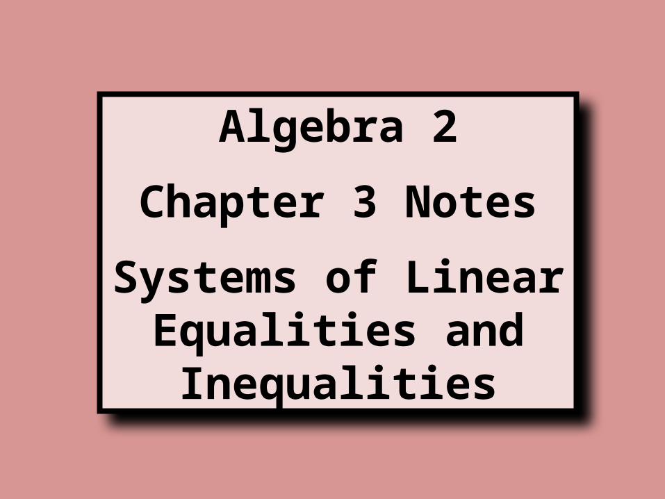
A system of 2 linear equations in 2 variables, x & y consists of 2 equations of the following form:
A x + B y = CD x + E y = F
A, B, C, D, E and F all represent constant values.
A solution of a system of linear equations in 2 variables is an ordered pair (x,y) that satisfies both equations.
Example 1: Checking solutions of a linear system. Are ( 2 , 2 ) and ( 0 , − 1 ) solutions of the following system:
3 x – 2 y = 2 x + 2 y = 6
3 x – 2 y = 2 x + 2 y = 6 3 ( 2 ) – 2 ( 2 ) = 2 ( 2 ) + 2 ( 2 ) = 66 – 4 = 2 2 + 4 = 62 = 2√ 6 = 6 √
3 x – 2 y = 2 x + 2 y = 6 3 ( 0 ) – 2 (− 1 ) = 2 ( 0 ) + 2 (− 1 ) = 60 + 2 = 2 0 − 2 = 62 = 2√ − 2 ≠ 6
Solution works for both
Solution does NOT work for both
Solving Linear Systems by Graphing 3.1

x 2 x – 3 y = 1 y x x + y = 3 y
0 2 (0) – 3 y = 1 – 3 y = 1
− 1 3
0 0 + y = 3 3
1 2
2 x – 3 (0) = 1 0 3 x + 0 = 3 0
• ••
•
•
2 x – 3 y = 1
x + y = 3
( 2 , 1 )
2 x – 3 y = 12 ( 2 ) – 3 ( 1 ) = 14 – 3 = 11 = 1 √
x + y = 32 + 1 = 3 3 = 3 √
Solving Linear Systems by Graphing 3.1
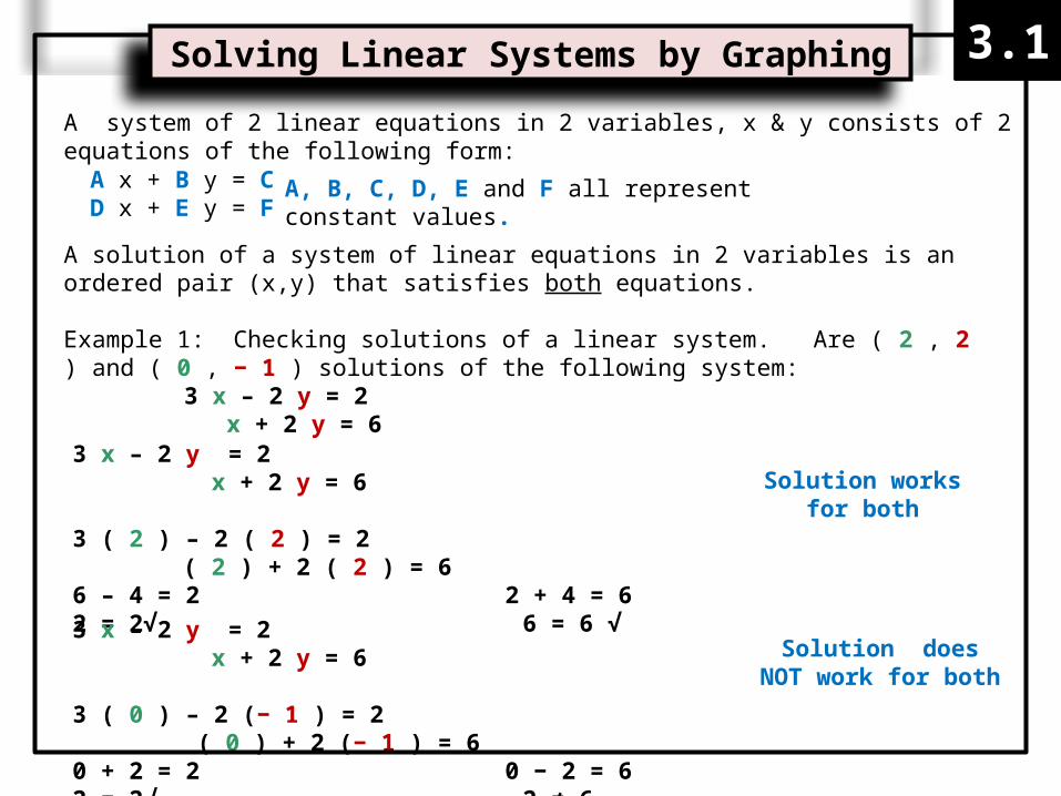
Graphical Interpretation Algebraic Interpretations
The graph of the system is a pair of lines that intersect in 1 point
The system has exactly 1 solution
The graph of the system is a single line The system has infinitely many solutions
The graph of the system is a pair of parallel lines so that there is no point of intersection
The system has no solution
Exactly 1 solution Infinitely many solutions No solution
Number of Solutions of a Linear System
3.1

Substitution Method:
1. Solve for one equation
2. Substitute the expression from step 1 into the other equation, then solve for the other variable
3. Substitute the value from step 2 into the revised equation from step 1, then solve
Example 1: 3 x + 4 y = − 4 [1st equation ] x + 2 y = 2 [2nd equation ]
1) Solve for x in equation 2 x + 2 y = 2 − 2 y − 2 yx = − 2 y + 2
2) Substitute 3 x + 4 y = − 43 (− 2 y + 2 ) + 4 y = − 4− 6 y + 6 + 4 y = − 4 − 2 y + 6 = − 4 − 2 y = − 10
y = 5
3). Use value for y to get x: x = − 2 y + 2 x = − 2 ( 5 ) + 2 x = − 10 + 2 = − 8
Check: 3 x + 4 y = − 43 (− 8 ) + 4 (5 ) = − 4 − 24 + 20 = − 4 − 4 = − 4 √
Solving Linear System Algebraically 3.2

7 x − 12 y = − 22 − 5 x + 8 y = 14
2 [ 7 x − 12 y = − 22 ] 3 [− 5 x + 8 y = 14 ]
14 x − 24 y = − 44 − 15 x + 24 y = 42 − 1 x = − 2
x = 2− 5 x + 8 y = 14− 5 (2) + 8 y = 14 − 10 + 8 y = 14 8 y = 24 y = 3 ( x , y )
( 2, 3 )
Check: 7 x − 12 y = − 227 ( 2 ) − 12 ( 3 ) = − 2214 − 36 = − 22 − 22 = − 22 √
Solving Linear System Algebraically
Linear Combination Method:
3.2
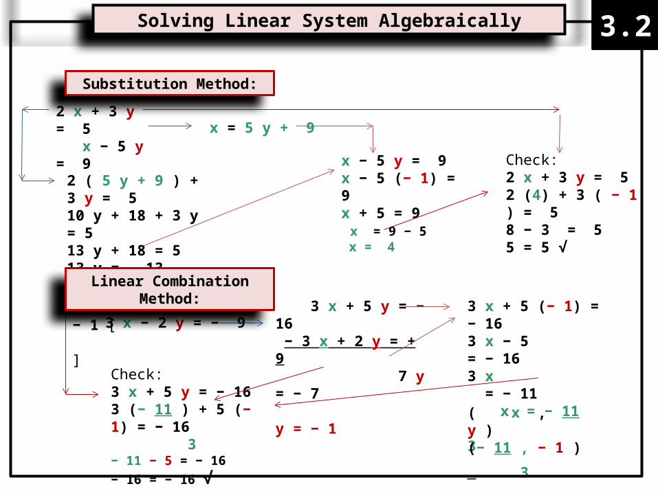
2 x + 3 y = 5 x − 5 y = 9 x = 5 y + 9
2 ( 5 y + 9 ) + 3 y = 510 y + 18 + 3 y = 513 y + 18 = 513 y = − 13 y = − 1
Check:2 x + 3 y = 52 (4) + 3 ( − 1 ) = 58 − 3 = 55 = 5 √
x − 5 y = 9 x − 5 (− 1) = 9x + 5 = 9 x = 9 − 5 x = 4
3 x + 5 y = − 163 x − 2 y = − 9− 1 [ ]
3 x + 5 y = − 16 − 3 x + 2 y = + 9 7 y = − 7 y = − 1
3 x + 5 (− 1) = − 163 x − 5 = − 163 x = − 11
x = − 11 3Check:
3 x + 5 y = − 163 (− 11 ) + 5 (− 1) = − 16 3− 11 − 5 = − 16
− 16 = − 16 √
( x , y )(− 11 , − 1 )
3
Solving Linear System Algebraically
Linear Combination Method:
Substitution Method:
3.2
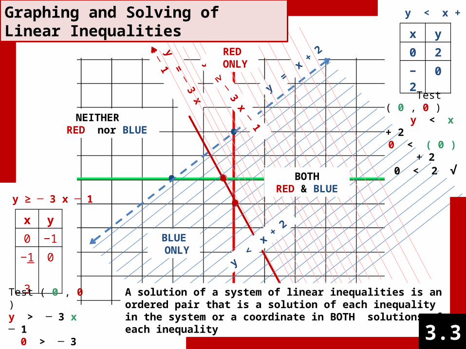
y ≥ ─ 3 x ─ 1
x y
0 −1
−1 3
0
Test ( 0 , 0 )y > ─ 3 x ─ 1 0 > ─ 3 ( 0 ) ─ 1
0 > ─ 1 √
y < x + 2
x y
0 2
− 2 0
Test ( 0 , 0 ) y < x + 2
0 < ( 0 ) + 20 < 2 √
••
y = ─ 3 x ─
1
•
•
y = x
+ 2
BLUE ONLY
BOTHRED & BLUE
NEITHER RED nor BLUE
A solution of a system of linear inequalities is an ordered pair that is a solution of each inequality in the system or a coordinate in BOTH solutions of each inequality
y < x
+ 2
y ≥ ─ 3 x ─
1
RED ONLY
Graphing and Solving of Linear Inequalities
3.3
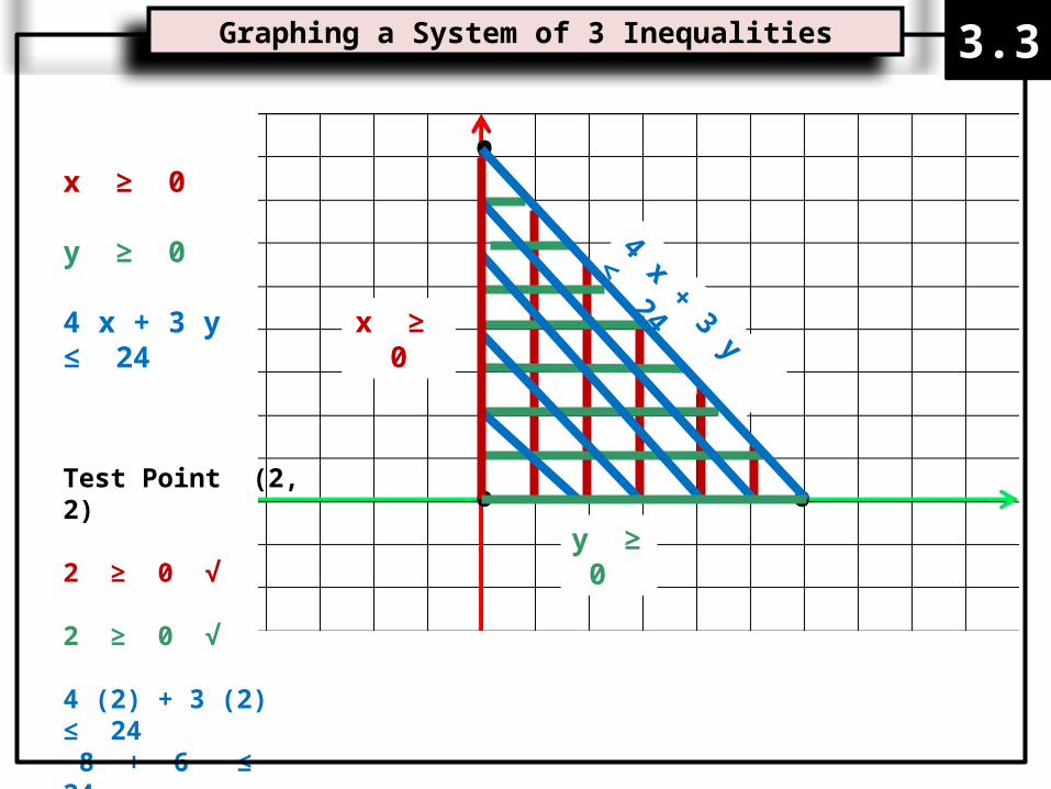
x ≥ 0
y ≥ 0
4 x + 3 y ≤ 24 x ≥ 0
y ≥ 0
4 x + 3 y ≤ 24
•
•
•Test Point (2, 2)
2 ≥ 0 √
2 ≥ 0 √
4 (2) + 3 (2) ≤ 24 8 + 6 ≤ 24 14 ≤ 24 √
Graphing a System of 3 Inequalities 3.3

Real life problems involve a process called OPTIMIZATION = finding the maximum or minimum value of some quantity.
Linear Programming is the process of optimizing a linear objective function subject to a system of linear inequalities called constraints. The graph of the system of constraints is called the feasible region.
Optimal solution of a Linear Programming problemIf an objective function has a maximum or a minimum value, then it must occur at a vertex of the feasible region. If the objective function is bounded,, then it has both a maximum and a minimum value.
• •
••
••
•
Bounded Region Unbounded Region
Linear Programming (a type of optimization)
3.4
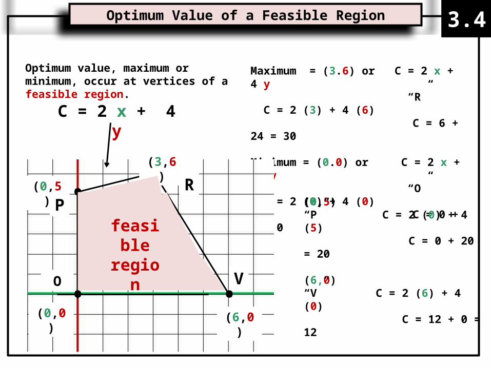
Optimum value, maximum or minimum, occur at vertices of a feasible region.
Maximum = (3.6) or C = 2 x + 4 y “R” C = 2 (3) + 4 (6)
C = 6 + 24 = 30
Minimum = (0.0) or C = 2 x + 4 y “O” C = 2 (0) + 4 (0)
C = 0 + 0 = 0
••
••
C = 2 x + 4 y
(0,5)
(0,0) (6,0)
(3,6)
O
PR
V
(0,5)“P” C = 2 (0) + 4 (5) C = 0 + 20 = 20
(6,0)“V” C = 2 (6) + 4 (0) C = 12 + 0 = 12
Optimum Value of a Feasible Region
feasible region
3.4

•
••(8,0)
(0,8)
(0,0)
Objective Function: C = 3 x + 4 y
x ≥ 0
Contraints: y ≥ 0
x + y ≤ 8 {
Vertices: C = 3 x + 4 y
(0,0) C = 3 (0) + 4 (0) = 0
(8,0) C = 3 (8) + 4 (0) = 24
(0,8) C = 3 (0) + 4 (8) = 32
minimum value
maximum value
Find Maximum and Minimum Values
Ex 1
3.4
•
•
•
(6,0)
(0,5)
(2,3)
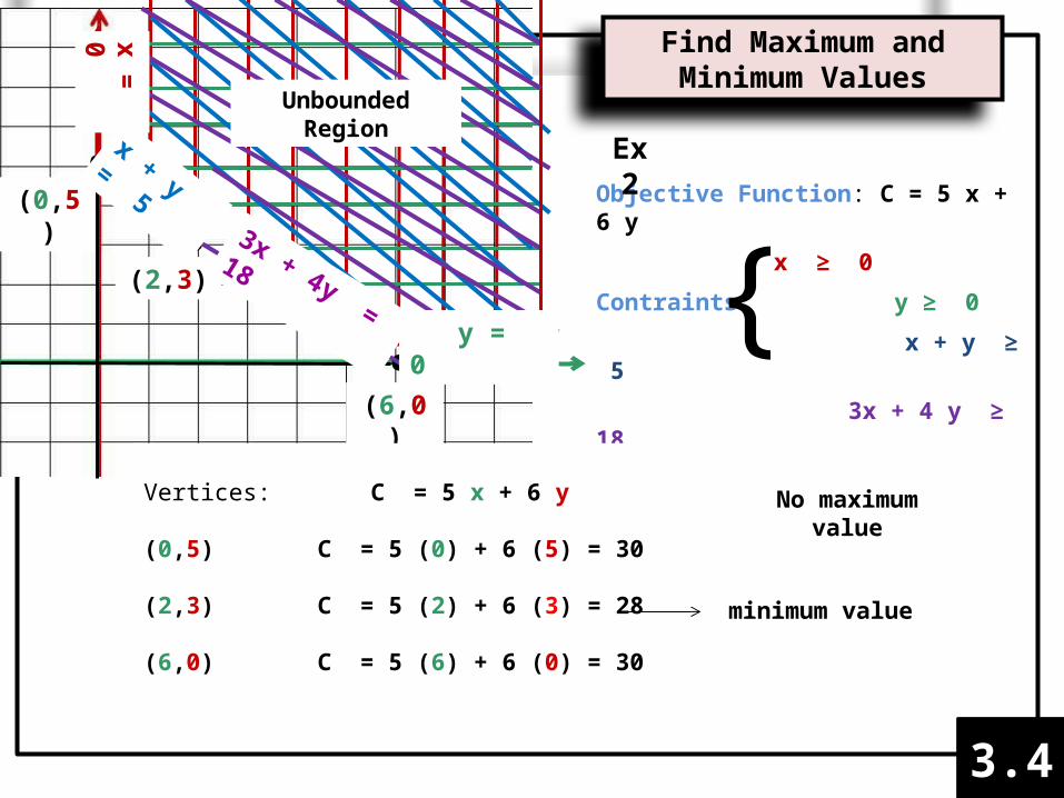
Objective Function: C = 5 x + 6 y
x ≥ 0
Contraints: y ≥ 0
x + y ≥ 5
3x + 4 y ≥ 18{
Vertices: C = 5 x + 6 y (0,5) C = 5 (0) + 6 (5) = 30
(2,3) C = 5 (2) + 6 (3) = 28
(6,0) C = 5 (6) + 6 (0) = 30
minimum value
No maximum value
x + y = 5 3x + 4y = 18
x = 0 Unbounded Region
y = 0
Find Maximum and Minimum Values
Ex 2
3.4
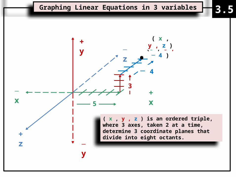
(5 , 3 , ─ 4 )+ y
+ x
+ z
─ z
─ x
─ y
( x , y , z )
•
5
─ 4
3
( x , y , z ) is an ordered triple, where 3 axes, taken 2 at a time, determine 3 coordinate planes that divide into eight octants.
Graphing Linear Equations in 3 variables 3.5
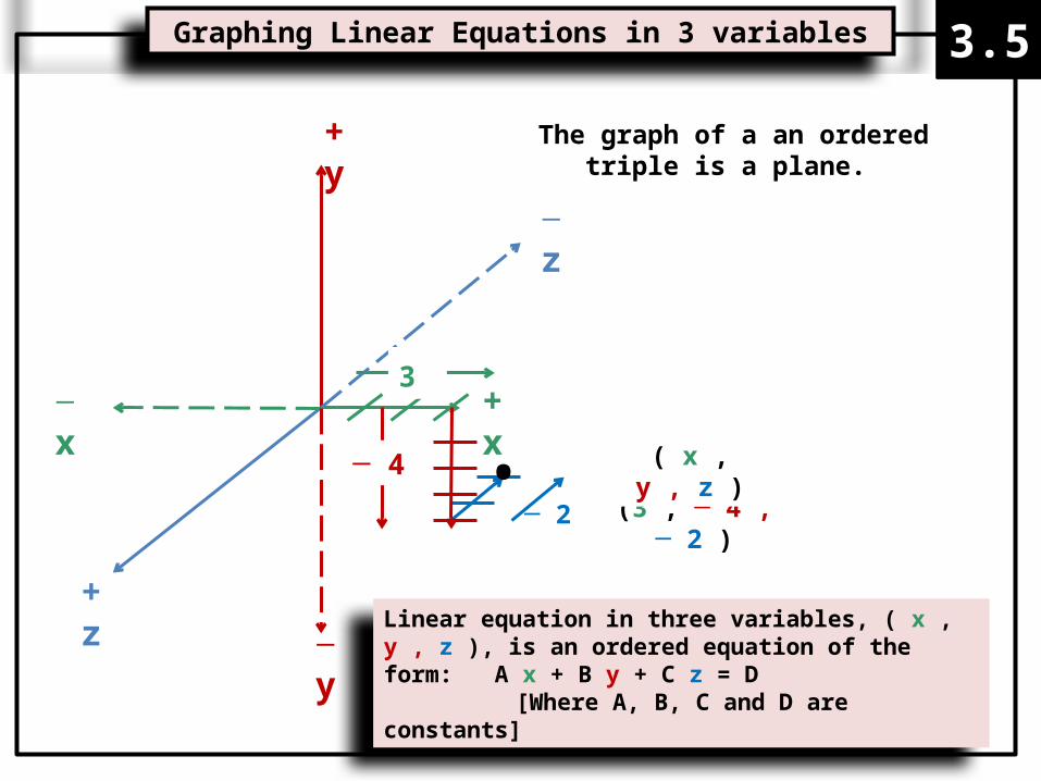
(3 , ─ 4 , ─ 2 )
+ y
+ x
+ z
─ z
─ x
─ y
( x , y , z )•
3
─ 4
─ 2
Linear equation in three variables, ( x , y , z ), is an ordered equation of the form: A x + B y + C z = D
[Where A, B, C and D are constants]
The graph of a an ordered triple is a plane.
Graphing Linear Equations in 3 variables 3.5
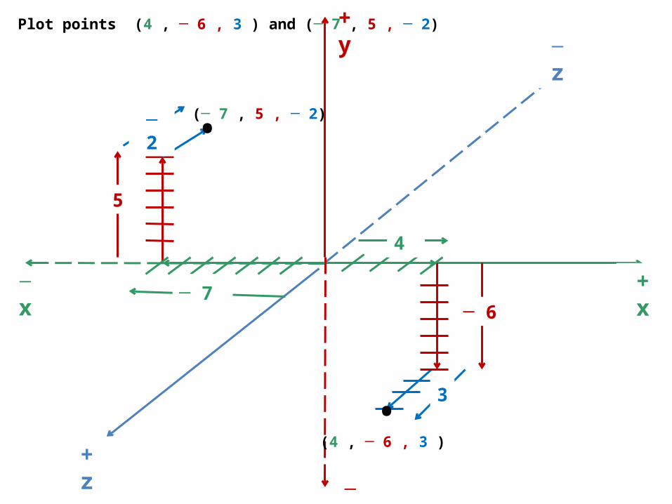
Plot points (4 , ─ 6 , 3 ) and (─ 7 , 5 , ─ 2) + y
+ x
+ z
─ z
─ x
─ y
4
•(4 , ─ 6 , 3 )
─ 7 ─ 6
5
3
─ 2 •(─ 7 , 5 , ─ 2)
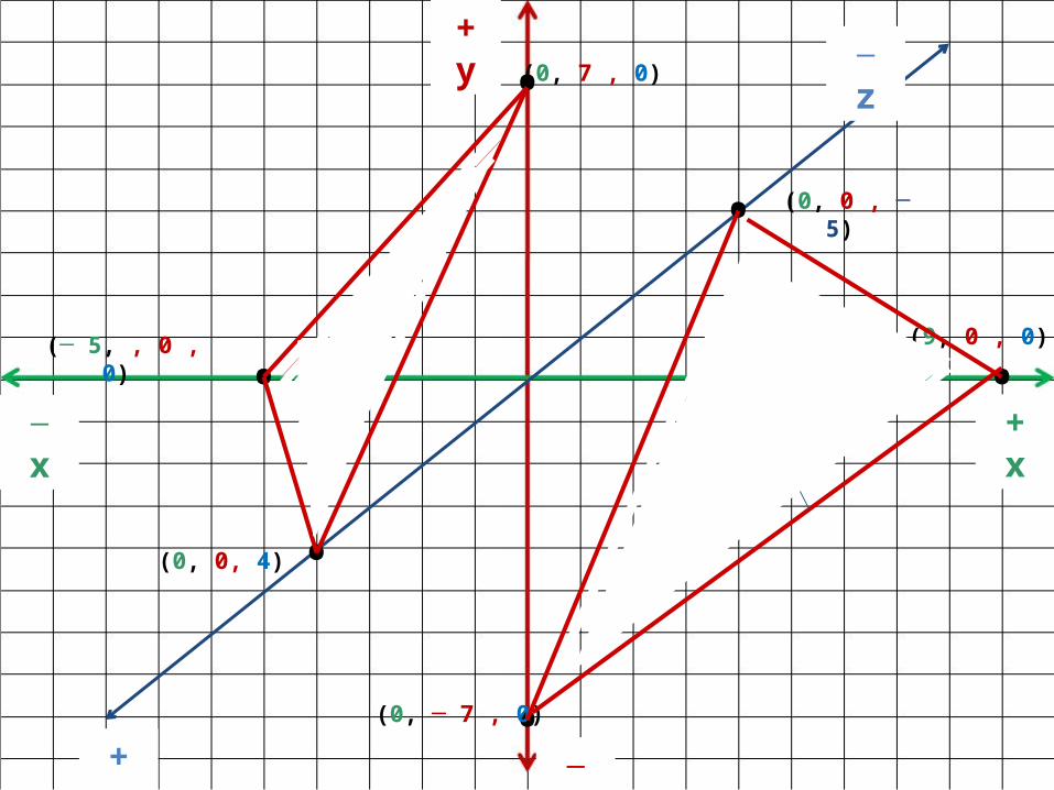
(0, 7 , 0)
(0, 0, 4)
•
•(─ 5, , 0 , 0)
•
• (0, 0 , ─ 5)
•(0, ─ 7 , 0)
•(9, 0 , 0)
+ y
─ y
+ x─ x
─ z
+ z

•
•
•
•
•
•
••
A
B C
D
EF
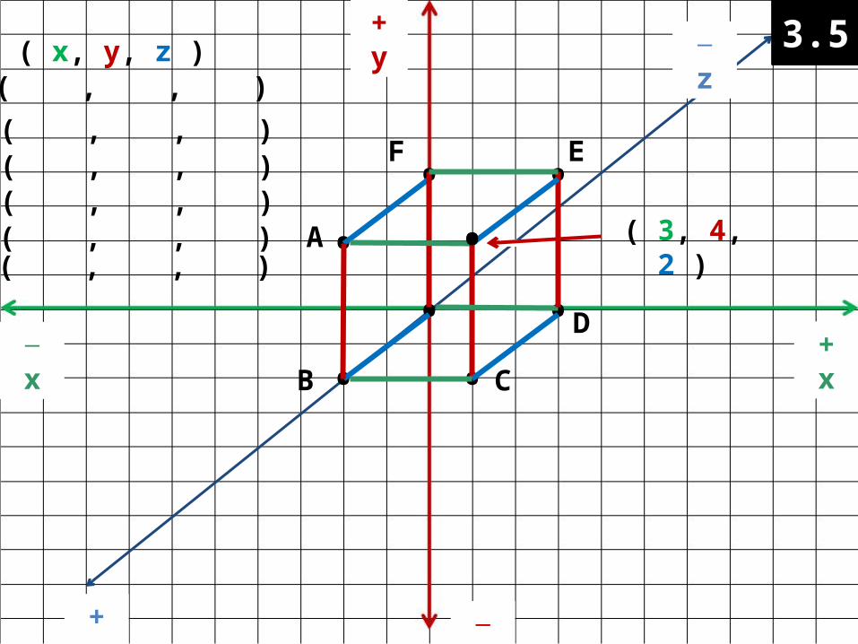
• ( 3, 4, 2 )
( x, y, z )A = ( , , )
B = ( , , )C = ( , , )D = ( , , )E = ( , , )F = ( , , )
+ y
─ y
+ x─ x
─ z
+ z
•
•
•
•
•
•
••
A
B C
D
EF
• ( 3, 4, 2 )
( x, y, z )A = ( , , )
B = ( , , )C = ( , , )D = ( , , )E = ( , , )F = ( , , )
+ y
─ y
+ x─ x
─ z
+ z
3.5
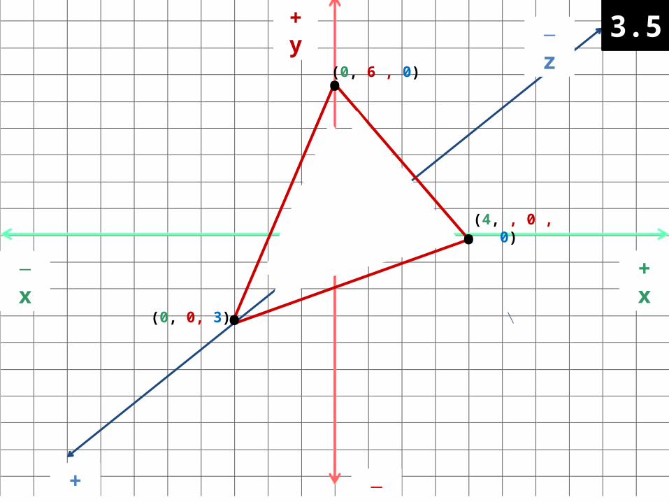
(0, 6 , 0)
(0, 0, 3)
(4, , 0 , 0)
•
•
+ y
─ y
+ x─ x
─ z
+ z
•
3.5
(0, 6 , 0)
(0, 0, 3)
(4, , 0 , 0)
•
•
+ y
─ y
+ x─ x
─ z
+ z
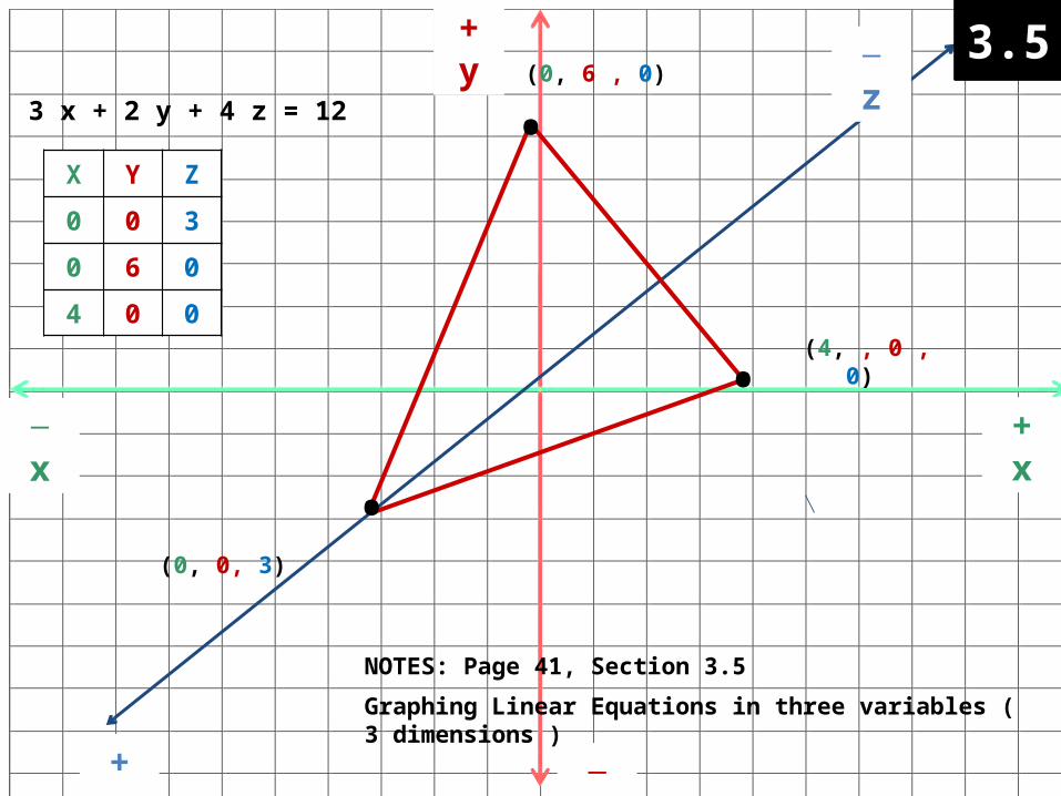
3 x + 2 y + 4 z = 12
X Y Z
0 0 3
0 6 0
4 0 0
•
NOTES: Page 41, Section 3.5
Graphing Linear Equations in three variables ( 3 dimensions )
3.5
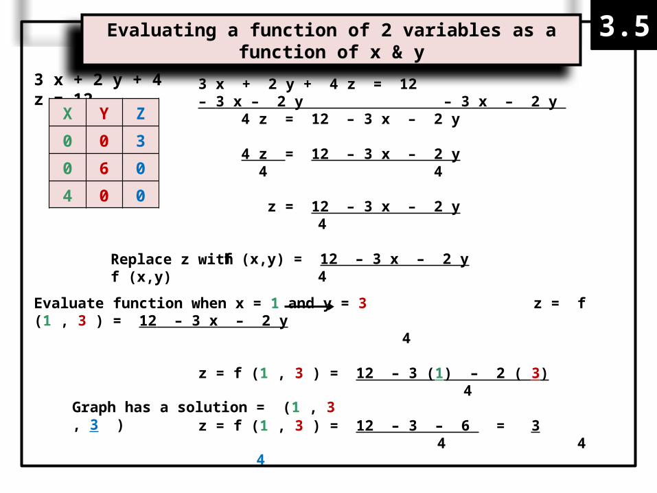
3 x + 2 y + 4 z = 12 – 3 x – 2 y – 3 x – 2 y
4 z = 12 – 3 x – 2 y
4 z = 12 – 3 x – 2 y 4 4
z = 12 – 3 x – 2 y 4
f (x,y) = 12 – 3 x – 2 y 4
3 x + 2 y + 4 z = 12
X Y Z
0 0 3
0 6 0
4 0 0
Replace z with f (x,y)
Evaluate function when x = 1 and y = 3 z = f (1 , 3 ) = 12 – 3 x – 2 y 4
z = f (1 , 3 ) = 12 – 3 (1) – 2 ( 3) 4
z = f (1 , 3 ) = 12 – 3 – 6 = 3 4 4
Graph has a solution = (1 , 3 , 3 ) 4
Evaluating a function of 2 variables as a function of x & y
3.5
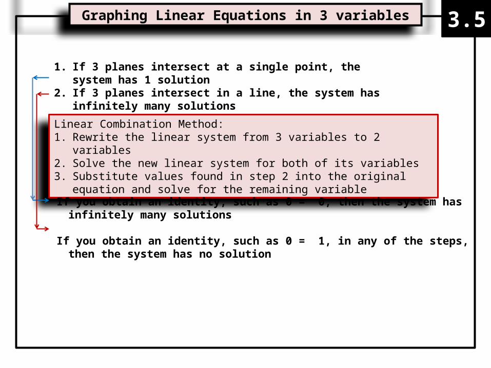
1. If 3 planes intersect at a single point, the system has 1 solution2. If 3 planes intersect in a line, the system has infinitely many solutions3. If 3 planes have no point of intersection, the system has no solution
Linear Combination Method:1. Rewrite the linear system from 3 variables to 2 variables2. Solve the new linear system for both of its variables3. Substitute values found in step 2 into the original equation and solve for the
remaining variable
If you obtain an identity, such as 0 = 0, then the system has infinitely many solutions
If you obtain an identity, such as 0 = 1, in any of the steps, then the system has no solution
Graphing Linear Equations in 3 variables 3.5

3 x + 2 y + 4 z = 112 x − y + 3 z = 45 x − 3 y + 5 z = − 1
{{
3 x + 2 y + 4 z = 112 (2 x − y + 3 z = 4)
→ →
− 3 ( 2 x − y + 3 z = 4 ) 5 x − 3 y + 5 z = − 1
→ →
3 x + 2 y + 4 z = 114 x − 2 y + 6 z = 8
− 6 x + 3 y − 9 z = − 12 5 x − 3 y + 5 z = − 1
7 x + 10 z = 19
− x − 4 z = − 13
7 x + 10 z = 19 7 ( − x − 4 z = − 13)
→ →
7x + 10 z = 19− 7x − 28 z = − 91
− 18 z = − 72z = 4
7x + 10 z = 19
7x + 10 (4) = 19 7x + 40 = 19 7x = − 21 x = − 3
2 x − y + 3 z = 4
y = 2
( x , y , z )(− 3 , 2 , 4 )
2 (− 3) − y + 3 (4) = 4− 6 − y + 12 = 4
− y + 6 = 4− y = − 2
Solving Systems Using Linear Combination ( 1 solution )
3.6