Algebra 1 Made Easy Handbook

Algebra 1 Made EasyHandbook

Next Generation Learning Standards Edition

By:Mary Ann Casey

B. S. Mathematics, M. S. Education

2018 Topical Review Book Company, Inc. All rights reserved.P. O. Box 328Onsted, MI. 49265-0328

This document may not, in whole or in part, be copied, photocopied, reproduced,translated, or reduced to any electronic medium or machine-readable form without prior consent in writing from Topical Review Book Corporation or its author.

AcknowledgementsNew York State has developed the Next Generation Learning Standards which arepresented in this book. Every author has people who help them and I am no exception. Kimberly Knisell, Director of Math and Science in the Hyde Park (NY) School District has been my primary consultant on processing the Next Generation Learning Standards. As always, thanks to Julieen Kane, graphicsdesigner and editor, who does an outstanding job in creating diagrams and formatting everything. Keith Williams, owner of my publisher, Topical Review Book Co., remains supportive and patient throughout the many changes in the content of the mathematics courses over the last 20 years. Thanks to all!

IntroductionThe content of this handbook is designed to coordinate with the New York State Next Generation Learning Standards for Algebra I. It is a reference of “how to do it” for the topics covered by the standards. The standards are taught with different approaches by different teachers, so my procedures may not match exactly with your teacher’s approach. Always use the methods presented by your teacher and use this book as a resource when needed. Additional material is included when I feel that it is mathematically appropriate to incorporate related content.Sincerely,

MaryAnn Casey, B.S. Mathematics, M.S. Education

Note on Fluency with Procedures Fluency with procedures (procedural fluency) means students are accurate, efficient, flexible, and know when and how to use them appropriately. Developing fluency requires understanding why and how a procedure works. Understanding makes learning procedures easier, less susceptible to common errors, less prone to forgetting, and easier to apply in new situations. Students also need opportunities to practice on a moderate number of carefully selected problems after they have established a strong conceptual foundation of the mathematical basis for the procedure.

Credit to: New York State Education Department, Next Generation Learning Standards.

Link:http://www.nysed.gov/common/nysed/files/nys-next-generation-mathematics-p-12-standards.pdf

Go to Algebra and find the blue notes on fluency.

____________________________________________________Algebra 1 Made Easy – Next Generation Learning Standards

Copyright 2018 Topical Review Book Inc. All rights reserved. 1

Unit 1

Foundations

• Algebraic Notation

• Real Numbers

• Numbers and Algebra

• Properties and Laws of Real Numbers and Polynomials

• Exponents

• Simplifying Radicals

• Pythagorean Theorem

___________________________________________________ Algebra 1 Made Easy – Next Generation Learning Standards Copyright 2018 Topical Review Book Company Inc. All rights reserved.

�

Algebraic N

otation

AlgebrAic NotAtioN Different notations are used to describe the elements or members of a set. Sometimes the elements are listed and in other cases a rule is used to define the members within the set.

DEFINItIoNSUniverse or Universal Set: The set of all possible elements available to form subsets.

Example The set of real numbers.

Set: A group of specific items within a universe.

Example The set of integers.

Subset: A set whose elements are completely contained in a larger set.

Example The set of even integers is a subset of the set of integers.

Complement of a Set: Symbols are A′, or AC. A′ contains the elements of the universal set that are not in Set A.

Example If the universe is whole numbers from 2 to 10 inclusive, and Set A = {2, 4, 6, 8, 10}, then A′ = {3, 5, 7, 9}.

Solution Set: All values of the variable(s) that satisfy an equation, inequality, system of equations, or system of inequalities.

Example In the set of real numbers, R , the solution set for the equation x2 = 9 is {3, –3} because 3 and –3 are solutions to that particular equation. Write the solution set: SS = {–3, 3}

SyMBoLS ∈ means “is an element of ”. Example 100 ∈ set of perfect squares.

∉ means “is not an element of ”. Example 3∉ set of perfect squares.

∅ or { } are symbols for the “empty set” or the “null set”. The empty set or null set has no elements in it.

Example If P is the set of negative numbers that are perfect squares of real numbers, then P = { } or P = ∅ .

Note: Do not use { } and ∅ together. {∅} means the set containing the element ∅. It does not mean the empty set or null set.

Notation: Ways to write the elements of a set.

1.1


Copyright 2018 Topical Review Book Inc. All rights reserved. �

Alg

ebra

ic N

otat

ion

Roster Form: A list of the elements in a set (Set A).

Example A = {2, 4, 6, 8, 10}

Set Builder Notation: A descriptive way to indicate the elements of a set.

Example The set of real numbers between 0 and 10, inclusive, would be written: {x : x ∈ R , 0 ≤ x ≤ 10} or {x | x ∈ R , 0 ≤ x ≤ 10}. The colon or the line both mean “such that.” This is read, “The set of all values of x such that x is a real number and 0 is less than or equal to x and x is less than or equal to 10.”

Inequality Notation: Inequality symbols are used to define the elements in the set. Symbols for exclusive are < and >. Symbols for inclusive are ≤ and ≥.

Examples –5 ≤ x < 7 means all values of x that are equal to or greater than –5 and less than 7. This includes –5 and excludes 7.

x < 3 or x ≥ 10 means the elements of the set that are less than 3 or the elements that are greater than or equal to 10. This excludes 3 and includes 10.

Interval Notation: Use ( , ) or [ , ] to indicate the end elements in a list of elements. Parentheses show the number is not included; brackets show that it is.

Example Set E = {x: 3 ≤ x< 6} would be written [3, 6). Set F = {x: 5 ≤ x≤ 8} would be written [5, 8]. Set G = {x: 0 < x< 5} would be written (0, 5). Examples

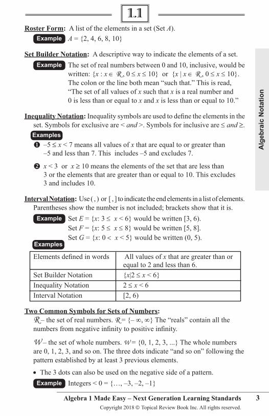
Elements defined in words All values of x that are greater than or equal to 2 and less than 6. Set Builder Notation {x|2 ≤ x< 6} Inequality Notation 2 ≤ x < 6 Interval Notation [2, 6)

two Common Symbols for Sets of Numbers: R – the set of real numbers. R = {– ∞, ∞} The “reals” contain all the numbers from negative infinity to positive infinity.

W – the set of whole numbers. W = {0, 1, 2, 3, ...} The whole numbers are 0, 1, 2, 3, and so on. The three dots indicate “and so on” following the pattern established by at least 3 previous elements.

• The 3 dots can also be used on the negative side of a pattern.

Example Integers < 0 = {…, –3, –2, –1}

1.1

�

Real N

umbers


1.2 reAl NUMberS

Sets of Numbers: All the sets below are part of the Set of Real Numbers, R . The REAL NUMBERS consist of all the numbers on a number line. If it were possible to place a point on the number line for each real number, the line would be completely filled in and extend forever (infinitely) in the negative and in the positive directions. (These are also referred to as negative infinity and positive infinity.) Real Numbers cannot be listed as a set. Write SS = {Real Numbers} if needed. The Real Numbers are composed of two major sets of numbers called RATIONAL numbers and IRRATIONAL numbers. Each of these sets contains several subsets.

the Set of Real Numbers Includes: • Positive Numbers = {x|x>0}. This is read, “The set of positive numbers contains all the values of xsuch that xis greater than zero.” In other words, all the numbers in this set are greater than zero.

• Negative Numbers = {x|x<0}. Read as: All the values of x less than zero

• Zero = {x|x=0}.

1. Rational numbeRs: Symbol is (Q ). Rational numbers are defined as the ratio of two integers and can be written in the form a

b where a and b are integers and b ≠ 0 (Division by zero is undefined). It is acceptable for b to be 1, so a rational number like 3 could be written 3

1. Rational numbers include these subsets.

a) Whole Numbers or W = {0, 1, 2, 3,...}. This is read, “The set of whole numbers contains the numbers 0, 1, 2, 3, and so on.” The “and so on” means that the pattern of numbers shown is to be continued.

�

Rea

l Num

bers


Copyright 2018 Topical Review Book Inc. All rights reserved.

b) Integers: Z = {..., –2, –1, 0, 1, 2,...} Subsetsofintegersinclude:

• Odd Integers: Positive or negative. Have a remainder when divided by 2. Odd Integers = {..., –5, –3, –1, 1, 3, 5,...} • Even Integers: Positive or negative. Divisible by 2. Include 0. Even Integers = {..., –6, –4, –2, 0, 2, 4, 6,...}

****Zero is an even integer, but it has no sign.**** • Positive Integers: {1, 2, 3, ...} [does not include 0] • Non-Negative Integers = {0, 1, 2, 3,...} [includes Positives & 0] • Negative Integers: {..., –3,–2,–1} [does not include 0] • Non-Positive Integers: {..., –3, –2, –1, 0} [includes Negatives & 0] • Natural Numbers or Counting Numbers: N = {1, 2, 3,...}

c) Fractions: A ratio of two integers with a denominator that is not equal to zero, like 2

3 or 54 .

d) terminating Decimals: Such as 0.24 which can be written 24 100 e) Repeating Decimals: Such as 0.37

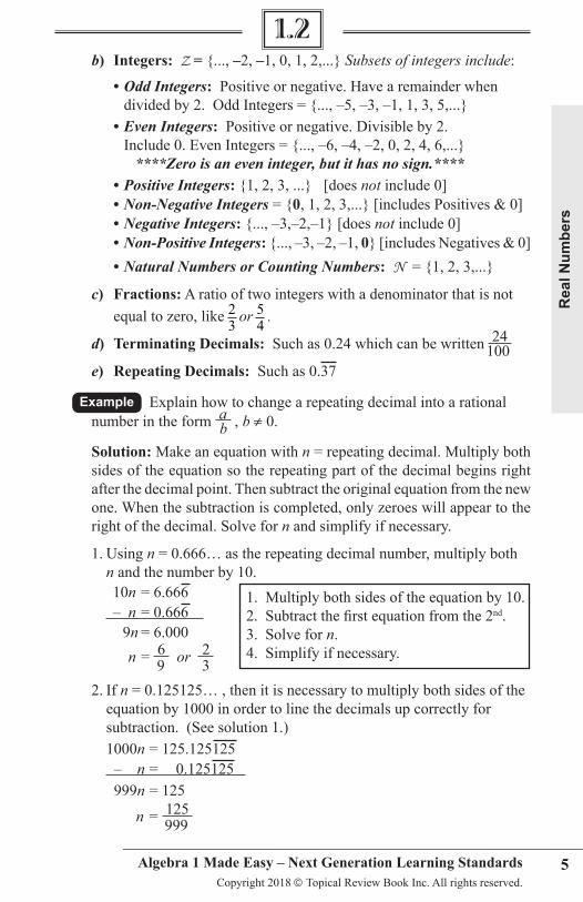
Example Explain how to change a repeating decimal into a rational number in the form a , b ≠ 0. b Solution: Make an equation with n = repeating decimal. Multiply both sides of the equation so the repeating part of the decimal begins right after the decimal point. Then subtract the original equation from the new one. When the subtraction is completed, only zeroes will appear to the right of the decimal. Solve for n and simplify if necessary.

1. Using n = 0.666… as the repeating decimal number, multiply both n and the number by 10. 10n = 6.666 – n = 0.666 9n = 6.000 n = 6 or 2 9 3 2. If n = 0.125125… , then it is necessary to multiply both sides of the equation by 1000 in order to line the decimals up correctly for subtraction. (See solution 1.) 1000n = 125.125125 – n = 0.125125 999n = 125

n = 125 999

1. Multiply both sides of the equation by 10.2. Subtract the first equation from the 2nd.3. Solve for n.4. Simplify if necessary.

1.2

�

Real N

umbers


Integrated Algebra Made Easy

� Copyright Topical Review Book Inc. All rights reserved.

2. Irrational Numbers: Whole numbers which cannot be expressed as the ratio of two intergers.

a) Non-repeating, nonterminating decimals like 0.354278...

b) The roots of numbers which do not calculate to a rational number. EThe square root of 12 which ≈ 3.4641016.

c) Pi or π is also irrational. The “π” button on the calculator must be used to compute formulas that contain π. Rounding to 3.14 is not permitted.

Note: When a calculator is used to work with irrational numbers, rounding is not permitted. To “show all work” write down on the paper all the digits in the calculator display. Leave the entire number in the calculator until the end of the problem. When directions say to round, it should be the final step of a problem.

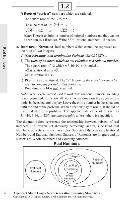
The diagram below represents the relationship of sets of real numbers. Theuni-versal set, shown by the rectangular box, is the Real Numbers. Subsets are shown ascircles. Subsets of the Reals are Irrational numbers and Rational numbers. Subsetsof Rationals are Integers and its subsets are Whole numbers and Counting numbers.

Real Numbers

IrrationalNumbers

RationalNumbers

Integers

WholeNumbers

CountingNumbers

f) Roots of “perfect” numbers which are rational. The square root of 25; 25 = 5. The cube root of –8; -83 = –2. 0 04. = 0.2 or 225 = 15. Note: There is an infinite number of rational numbers and they cannot be written as a listed set. Write SS = {rational numbers} if needed.

�. iRRational numbeRs: Real numbers which cannot be expressed as the ratio of two integers. a) Non-repeating,non-terminating decimals like 0.354278... b) The roots of numbers which do not calculate to a rational number. The square root of 12 which ≈ 3.4641016 (rounded). 2 is irrational as is 5. 163 is irrational also. c) Pi or π is also irrational. The “π” buttononthecalculatormustbe usedtocomputeformulasthatcontain π. Rounding to 3.14 is not permitted.

Note: When a calculator is used to work with irrational numbers, rounding is not permitted. To “show all work” write down on the paper all the digits in the calculator display. Leave the entire number in the calculator until the end of the problem. When directions say to round, it should be the final step of a problem. The approximate value of π, such as 3.1416, 3.14, or 22/7, are unacceptable unless otherwise specified.

The diagram below represents the relationship between subsets of real numbers. The universal set, shown by the rectangular box, is the set of Real Numbers. Subsets are shown as circles. Subsets of the Reals are Irrational Numbers and Rational Numbers. Subsets of Rationals are Integers and its subsets are Whole Numbers and Counting Numbers.

1.2

Whole Numbers

�0

Algebraic Term

inology and Expressions


Identifying Parts of Algebraic Expressions: It is necessary to identify individual parts of complicated expressions in order to analyze the method needed for proceeding with a problem.

Examples 5x2 : 5 is the coefficient, x is the variable. Additionally 5 and x are both factors of the term. 2 is the exponent that is to be applied to x. Other ways to write this might be 5(x2) or 5(x)(x). 6x2 + 7 : This is a binomial expression. 6x2 and 7 are both terms of the expression. 7 is a constant. 2 is an exponent applied to the variable, x. 6 is the coefficient of the variable. 4(3x2 + 5) : 4 is a factor in this expression. (3x2 + 5) is a binomial factor. 5x (x + 2)2 : 5x is a factor. (x + 2) is a binomial factor that is to be raised to the 2nd power. 2 is the exponent and it is applied only to the binomial factor (x + 2). (x + 1)(x – 2)2 : (x + 1) is a binomial factor. (x – 2) is another binomial factor. The exponent of 2 is to be applied only to (x – 2). �R(x– l)t: R and (x– 1) are both factors and t is the exponent that is applied to (x– 1). Multiply (x– 1) by (x – 1) ttimes. Then multiply that answer by R.

Equivalent Forms of Expressions: It is often necessary to rewrite an expression or equation in order to solve problems. The properties and laws of real numbers also apply to polynomials. Sometimes expanding the expression is appropriate and in other cases simplifying the expression is needed. The following are some examples written in equivalent forms.

Examples (x +2)(x – 5) can be written as x2 – 3x – 10.

9 3x is equivalent to 3x x .

5x(x+ 2)2 can be multiplied out and written 5x(x2 + 4x+ 4) which is equivalent to 5x3 + 20x2 + 20x.

6x2 + 12x– 18 is equivalent to 6(x2 +2x– 3) which can also be written 6(x+ 3)(x – 1). x4 – y4 is the difference of 2 perfect squares. It can be rewritten as (x2 – y2)(x2 + y2). Since (x2 – y2) is still the difference of two perfect squares, this can be factored further as (x – y)(x + y)(x2 + y2). �64x2 + 32x + 4 is equivalent to (8x)2 + 4(8x) + 4

3.2AlgebrAic expreSSioNS

Ope

ratio

ns w

ith P

olyn

omia

ls

�1____________________________________________________

Algebra 1 Made Easy – Next Generation Learning StandardsCopyright 2018 Topical Review Book Inc. All rights reserved.

The properties and laws of real numbers can be applied to polynomials.

Closure: Polynomials are closed under the operations of addition, subtraction, and multiplication.

Addition: Remove any parenthesis using the distributive property if needed. (You can always put a “1” in front of a ( ) if it is easier for you.) Then combine like terms.

Example 2(x2 + 3x – 4) + 3x2 – 4x Steps 1) Distribute the 2: 2x2 + 6x – 8 + 3x2 – 4x 2) Collect like terms: 5x2 + 2x – 8

Example x3 + 2x – 3 + 3(x2 – 5) Steps 1) Distribute the 3: x3 + 2x – 3 + 3x2 – 15 2) Collect like terms: x3 + 3x2 + 2x – 18

Subtraction: Multiply the terms in the polynomial to be subtracted by –1 (use the distributive property). This removes the parenthesis and takes care of the SIGN CHANGES. Then ADD by combining like terms.

Example (3x – 2) + (5x – y) – (2x – 4) Steps 1) Put in “1’s”: 1(3x – 2) + 1(5x – y) – 1(2x – 4) 2) Use the distributive property: 3x – 2 + 5x – y – 2x + 4 3) Simplify or collect like terms: 6x – y + 2

Example From the sum of (x + 2y) and (2x – y), subtract (3x – y). Steps 1) Put brackets around the sum first: [(x + 2y) + (2x – y)] – (3x – y) 2) Simplify inside the bracket: [x+ 2x + 2y – y] – (3x – y) 3) Put in “1’s”: 1(3x + y) –1(3x – y) 4) Use the distributive property: 3x + y – 3x + y 5) Simplify or collect like terms: 2y

Example Subtract 5x – 2y from 12x – 5 Steps 1) Put the “from” expression first: (12x – 5) – (5x – 2y) 2) Put in “1’s”: 1(12x – 5) –1(5x – 2y) 3) Use the distributive property: 12x – 5 – 5x + 2y 4) Simplify or collect like terms: 7x + 2y – 5****EXPONENTSDONOTCHANGEINADDITION/SUBTRACTION****

3.3operations With polynomials

FLU

EN

CY

FLU

EN

CY

��

Operations w

ith Polynomials


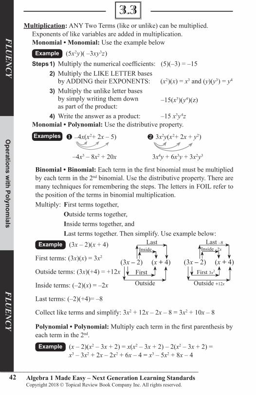
Multiplication: ANY Two Terms (like or unlike) can be multiplied. Exponents of like variables are added in multiplication. Monomial • Monomial: Use the example below

Example (5x2y)( –3xy3z) Steps 1) Multiply the numerical coefficients: (5)(–3) = –15 2) Multiply the LIKE LETTER bases by ADDING their EXPONENTS: (x2)(x) = x3 and (y)(y3) = y4

3) Multiply the unlike letter bases by simply writing them down as part of the product:

–15(x3)(y4)(z)

4) Write the answer as a product: –15 x3y4z Monomial • Polynomial: Use the distributive property.

Examples –4x(x2+ 2x– 5) 3x2y(x2+ 2x+ y2)

–4x3 – 8x2+ 20x 3x4y + 6x3y+ 3x2y3

3.3

Binomial • Binomial: Each term in the first binomial must be multiplied by each term in the 2nd binomial. Use the distributive property. There are many techniques for remembering the steps. The letters in FOIL refer to the position of the terms in binomial multiplication. Multiply: First terms together, outside terms together, Inside terms together, and Last terms together. Then simplify. Use example below:

Example (3x – 2)(x + 4)

First terms: (3x)(x) = 3x2

Outside terms: (3x)(+4) = +12x

Inside terms: (–2)(x) = –2x

Last terms: (–2)(+4)= –8

Collect like terms and simplify: 3x2 + 12x – 2x – 8 = 3x2 + 10x – 8

Polynomial • Polynomial: Multiply each term in the first parenthesis by each term in the 2nd.

Example (x – 2)(x2 – 3x + 2) = x(x2 – 3x + 2) – 2(x2 – 3x + 2) = x3 – 3x2 + 2x – 2x2 + 6x – 4 = x3 – 5x2 + 8x – 4

First 3x2

Outside

Last

(3x – 2) (x + 4) (3x – 2) (x + 4)First

InsideLast –8

Inside –2x

Outside +12x

FLU

EN

CY

FLU

EN

CY

Ope

ratio

ns w

ith P

olyn

omia

ls

��____________________________________________________


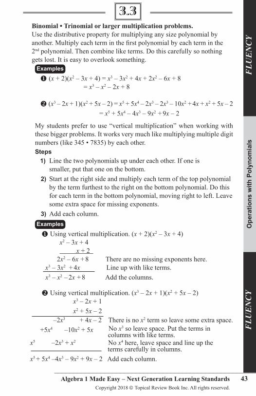
3.3 Binomial • trinomial or larger multiplication problems. Use the distributive property for multiplying any size polynomial by another. Multiply each term in the first polynomial by each term in the 2nd polynomial. Then combine like terms. Do this carefully so nothing gets lost. It is easy to overlook something.

Examples (x + 2)(x2 – 3x + 4) = x3 – 3x2 + 4x + 2x2 – 6x + 8 = x3 – x2 – 2x + 8

(x3 – 2x + 1)(x2 + 5x – 2) = x5 + 5x4 – 2x3 – 2x3 – 10x2 + 4x + x2 + 5x – 2 = x5 + 5x4 – 4x3 – 9x2 + 9x – 2 My students prefer to use “vertical multiplication” when working with these bigger problems. It works very much like multiplying multiple digit numbers (like 345 • 7835) by each other. Steps 1) Line the two polynomials up under each other. If one is smaller, put that one on the bottom. 2) Start at the right side and multiply each term of the top polynomial by the term furthest to the right on the bottom polynomial. Do this for each term in the bottom polynomial, moving right to left. Leave some extra space for missing exponents. 3) Add each column.

Examples Using vertical multiplication. (x + 2)(x2 – 3x + 4) x2 – 3x + 4 x + 2 2x2 – 6x + 8 There are no missing exponents here. x3 – 3x2 + 4xLine up with like terms. x3 – x2 – 2x + 8 Add the columns.

Using vertical multiplication. (x3 – 2x + 1)(x2 + 5x – 2) x3 – 2x + 1 x2 + 5x – 2 –2x3 + 4x – 2 There is no x2 term so leave some extra space. +5x4 –10x2 + 5x No x3 so leave space. Put the terms in x5 –2x3 + x2

columns with like terms.

No x4 here, leave space and line up the

terms carefully in columns.

x5 + 5x4 –4x3 – 9x2 + 9x – 2 Add each column.

FLU

EN

CY

FLU

EN

CY

��

Factoring


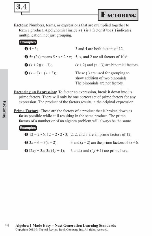
Factors: Numbers, terms, or expressions that are multiplied together to form a product. A polynomial inside a ( ) is a factor if the ( ) indicates multiplication, not just grouping.

Examples

4 • 3; 3 and 4 are both factors of 12.

5x (2x) means 5 • x • 2 • x; 5, x, and 2 are all factors of 10x2.

(x + 2)(x – 3); (x + 2) and (x – 3) are binomial factors.

(x – 2) + (x + 3); These ( ) are used for grouping to show addition of two binomials. The binomials are not factors.

Factoring an Expression: To factor an expression, break it down into its prime factors. There will only be one correct set of prime factors for any expression. The product of the factors results in the original expression.

Prime Factors: These are the factors of a product that is broken down as far as possible while still resulting in the same product. The prime factors of a number or of an algebra problem will always be the same.

Examples

12 = 2 • 6; 12 = 2 • 2 • 3; 2, 2, and 3 are all prime factors of 12.

3x + 6 = 3(x + 2); 3 and (x + 2) are the prime factors of 3x + 6.

l2xy + 3x: 3x (4y + 1); 3 and x and (4y + 1) are prime here.

3.4FActoriNg

Fact

orin

g

��____________________________________________________


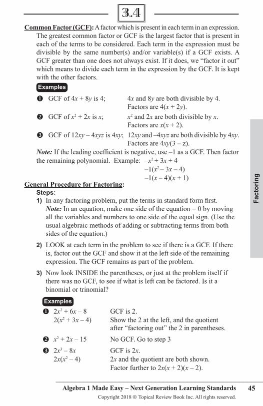
Common Factor (GCF): A factor which is present in each term in an expression. The greatest common factor or GCF is the largest factor that is present in each of the terms to be considered. Each term in the expression must be divisible by the same number(s) and/or variable(s) if a GCF exists. A GCF greater than one does not always exist. If it does, we “factor it out” which means to divide each term in the expression by the GCF. It is kept with the other factors.

Examples

GCF of 4x + 8y is 4; 4x and 8y are both divisible by 4. Factors are 4(x + 2y). GCF of x2 + 2x is x; x2 and 2x are both divisible by x. Factors are x(x + 2). GCF of 12xy – 4xyz is 4xy; 12xy and –4xyz are both divisible by 4xy. Factors are 4xy(3 – z). Note: If the leading coefficient is negative, use –1 as a GCF. Then factor the remaining polynomial. Example: –x2 + 3x + 4 –1(x2 – 3x – 4) –1(x – 4)(x + 1)General Procedure for Factoring: Steps: 1) In any factoring problem, put the terms in standard form first. Note: In an equation, make one side of the equation = 0 by moving all the variables and numbers to one side of the equal sign. (Use the usual algebraic methods of adding or subtracting terms from both sides of the equation.) 2) LOOK at each term in the problem to see if there is a GCF. If there is, factor out the GCF and show it at the left side of the remaining expression. The GCF remains as part of the problem. 3) Now look INSIDE the parentheses, or just at the problem itself if there was no GCF, to see if what is left can be factored. Is it a binomial or trinomial?

Examples 2x2 + 6x – 8 GCF is 2. 2(x2 + 3x – 4) Show the 2 at the left, and the quotient after “factoring out” the 2 in parentheses.

x2 + 2x – 15 No GCF. Go to step 3

2x3 – 8x GCF is 2x. 2x(x2 – 4) 2x and the quotient are both shown. Factor further to 2x(x + 2)(x – 2).

3.4

��

Factoring


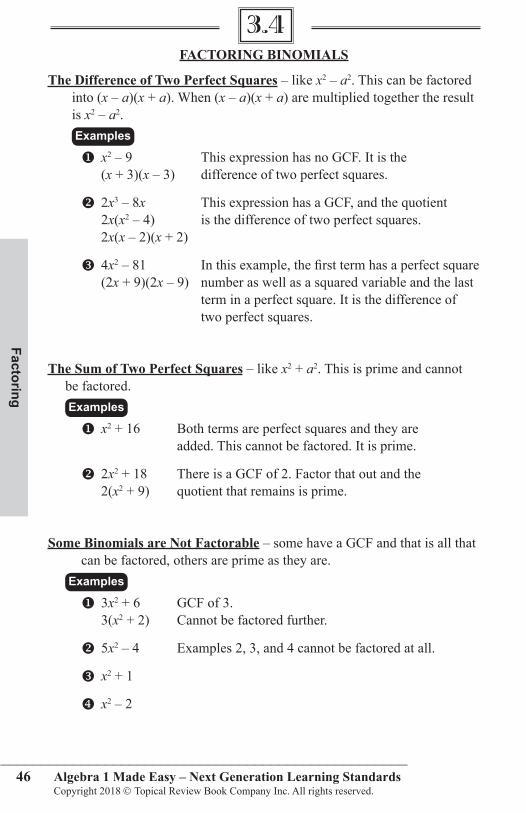
FACtoRING BINoMIALS

the Difference of two Perfect Squares – like x2 – a2. This can be factored into (x – a)(x + a). When (x – a)(x + a) are multiplied together the result is x2 – a2.

Examples

x2 – 9 This expression has no GCF. It is the (x + 3)(x – 3) difference of two perfect squares.

2x3 – 8x This expression has a GCF, and the quotient 2x(x2 – 4) is the difference of two perfect squares. 2x(x – 2)(x + 2)

4x2 – 81 In this example, the first term has a perfect square (2x + 9)(2x – 9) number as well as a squared variable and the last term in a perfect square. It is the difference of two perfect squares.

the Sum of two Perfect Squares – like x2 + a2. This is prime and cannot be factored.

Examples

x2 + 16 Both terms are perfect squares and they are added. This cannot be factored. It is prime.

2x2 + 18 There is a GCF of 2. Factor that out and the 2(x2 + 9) quotient that remains is prime.

Some Binomials are Not Factorable – some have a GCF and that is all that can be factored, others are prime as they are.

Examples

3x2 + 6 GCF of 3. 3(x2 + 2) Cannot be factored further.

5x2 – 4 Examples 2, 3, and 4 cannot be factored at all.

x2 + 1

x2 – 2

3.4

8�

Solving Systems G

raphically


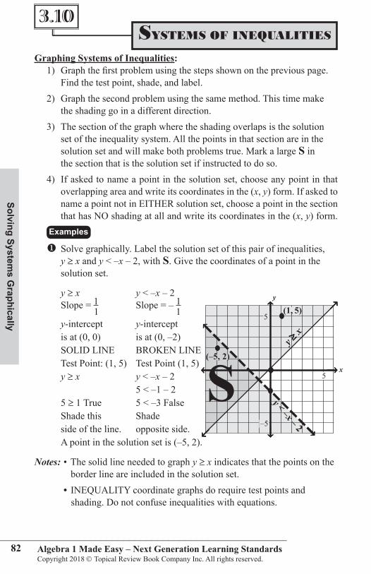
Graphing Systems of Inequalities: 1) Graph the first problem using the steps shown on the previous page. Find the test point, shade, and label. 2) Graph the second problem using the same method. This time make the shading go in a different direction. 3) The section of the graph where the shading overlaps is the solution set of the inequality system. All the points in that section are in the solution set and will make both problems true. Mark a large S in the section that is the solution set if instructed to do so. 4) If asked to name a point in the solution set, choose any point in that overlapping area and write its coordinates in the (x, y) form. If asked to name a point not in EITHER solution set, choose a point in the section that has NO shading at all and write its coordinates in the (x, y) form.

Examples Solve graphically. Label the solution set of this pair of inequalities, y ≥ x and y < –x – 2, with S. Give the coordinates of a point in the solution set.

y ≥ x y < –x – 2 Slope = 1 Slope = – 1 1 1 y-intercept y-intercept is at (0, 0) is at (0, –2) SOLID LINE BROKEN LINE Test Point: (1, 5) Test Point (1, 5) y ≥ x y < –x – 2 5 < –1 – 2 5 ≥ 1True 5 < –3 False Shade this Shade side of the line. opposite side. A point in the solution set is (–5, 2).

Notes: • The solid line needed to graph y ≥ x indicates that the points on the border line are included in the solution set. • INEQUALITY coordinate graphs do require test points and shading. Do not confuse inequalities with equations.

77Integrated Algebra Made Easy

Copyright Topical Review Book Inc. All rights reserved.

x

y

yx

y < –x – �

Example

Graphing Systems of Inequalities:

1) Graph one problem as shown on the previous page. Find the test point, shade,and label.

2) Graph the 2nd problem - same method. This time make the shading go in adifferent direction.

3) The section of the graph where the shading overlaps is the solution set of theinequality system. All the points in that section are in the solution set and willmake both problems true. Mark a large “S” in the section that is the solutionset if instructed to do so.

4) If asked to name a point in the solution set, choose any point in thatoverlapping area and write its coordinates in the (x,y) form. If asked to namea point not in EITHER solution set, choose a point in the section that has NOshading at all and write its coordinates in the (x,y) form.

Solve graphically. Label the solution set of this pair of inequalities,y x and y –x – 2, with S. Give the coordinates of a point in the solution set.

y x y –x – 2

Slope = 11 Slope = – 1

1

y-intercept y-interceptis at (0, 0) is at (0, –2)SOLID LINE* BROKEN LINE

Test Point: (1, 5) Test Point (1, 5)

y x y –x – 2

5 < –1 – 2

5 x True 5 < –3 FalseShade this Shadeside of the line. opposite side.

A point in the solution set is (–5, 2)

Note:The solid line needed to graph y x indicates that the points on the borderline are included in the solution set.

Note: INEQUALITY coordinate graphs dorequiretestpointsandshading. Donot confuse inequalities with equations (See page 58).

(–�, �)

(1, �)5

5

–5

S

3.10SySteMS oF iNeqUAlitieS

Solv

ing

Syst

ems

Gra

phic

ally

8�____________________________________________________


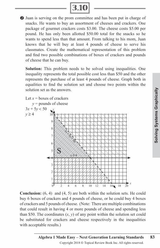
Juan is serving on the prom committee and has been put in charge of snacks. He wants to buy an assortment of cheeses and crackers. One package of gourmet crackers costs $3.00. The cheese costs $5.00 per pound. He has only been allotted $50.00 total for the snacks so he wants to spend less than that amount. From talking to his mom, Juan knows that he will buy at least 4 pounds of cheese to serve his classmates. Create the mathematical representation of this problem and find two possible combinations of boxes of crackers and pounds of cheese that he can buy.

Solution: This problem needs to be solved using inequalities. One inequality represents the total possible cost less than $50 and the other represents the purchase of at least 4 pounds of cheese. Graph both in equalities to find the solution set and choose two points within the solution set as the answers.

Let x = boxes of crackers y = pounds of cheese 3x + 5y < 50 y ≥ 4

Conclusion: (6, 4) and (4, 5) are both within the solution sets. He could buy 6 boxes of crackers and 4 pounds of cheese, or he could buy 4 boxes of crackers and 5 pounds of cheese. (Note: There are multiple combinations that could result in having 4 or more pounds of cheese and spending less than $50. The coordinates (x, y) of any point within the solution set could be substituted for crackers and cheese respectively in the inequalities with acceptable results.)

3.10

10

9

8

7

6

5

4

3

2

1

0 2 4 6 8 10 12 14 16 18 20

y

x

3x + 5y < 50

S y ≥ 4 •

8�

Solving Inequalities With C

onstraints


Constraint: A restriction, boundary, or limit that regulates possible outcomes.

Working with linear polynomials can help find the possible maximum or minimum values in problem solving. Systems of linear inequalities are used in real world situations where it is necessary to combine several resources to produce a maximum or minimum result. Using linear inequalities provides a feasible region or area which shows all the possible outcomes of the process based on an objective equation or function which defines the purpose of the problem. These outcomes are restricted by the boundary lines of the inequalities. The restrictions are called constraints. The maximum and minimum output values are found at the intersections of the lines that are the boundaries of the inequalities. This process is also called linear programming. Steps: 1) Determine what the purpose of the problem is and write a linear equation to represent it. This equation is often called the objective equation or the optimization equation. 2) Write inequalities that represent the desired solution of each component of the problem. These are called restrictions, or constraints. 3) Graph each inequality on a coordinate plane and indicate the correct solution areas. Each inequality line is the boundary of that part of the solution. The portion of the graph where all of the solutions overlap is called the feasible area or region. 4) Use the linear equations as a system of equations to find the points of intersection of the boundary lines. These points will be the corners of the feasible region. 5) Substitute the coordinates of each of the points of intersection in the “Objective Equation.” The coordinates that provide the highest or lowest value when substituted in the objective equation are the x and yvalues of the solution. 6) Write a conclusion.

The first example on the next page demonstrates the development of a problem where the individual parts of the problem are already defined as mathematical statements. In the second example, the necessary mathematical statements must be developed from an application.

3.11SolviNg liNeAr probleMS

With coNStrAiNtS

Solv

ing

Ineq

ualit

ies

With

Con

stra

ints

8�____________________________________________________


Example

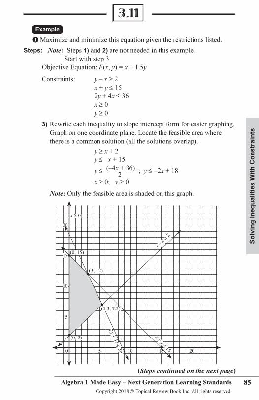
Maximize and minimize this equation given the restrictions listed. Steps: Note: Steps 1) and 2) are not needed in this example. Start with step 3. Objective Equation: F(x, y) = x + 1.5y

Constraints: y – x ≥ 2 x + y ≤ 15 2y + 4x ≤ 36 x ≥ 0 y ≥ 0 3) Rewrite each inequality to slope intercept form for easier graphing. Graph on one coordinate plane. Locate the feasible area where there is a common solution (all the solutions overlap). y ≥ x + 2 y ≤ –x + 15 y ≤ (–4x + 36) ; y ≤ –2x + 18 2 x ≥ 0; y ≥ 0

Note: Only the feasible area is shaded on this graph.

(Steps continued on the next page)

•

20

15

10

5

0 5 10 15 20

•

•

•

•

(0, 15)

(0, 2)

(3, 12)

(5.3, 7.3)

y–x ≥

2

2y+ 4x ≤ 36

x+ y ≤ 15

3.11

x ≥ 0

8�


onstraints


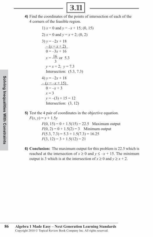
4) Find the coordinates of the points of intersection of each of the 4 corners of the feasible region. 1) x = 0 and y = –x + 15; (0, 15) 2) x = 0 and y = x + 2; (0, 2) 3) y = –2x + 18 – (y = x + 2) 0 = –3x + 16 x = 16 or 5.3 3 y = x + 2; y = 7.3 Intersection: (5.3, 7.3) 4) y = –2x + 18 – (y = –x + 15) 0 = –x + 3 x = 3 y = –(3) + 15 = 12 Intersection: (3, 12) 5) Test the 4 pair of coordinates in the objective equation. F(x, y) = x + 1.5y F(0, 15) = 0 + 1.5(15) = 22.5 Maximum output F(0, 2) = 0 + 1.5(2) = 3 Minimum output F(5.3, 7.3) = 5.3 + 1.5(7.3) = 16.25 F(3, 12) = 3 + 1.5(12) = 21 6) Conclusion: The maximum output for this problem is 22.5 which is reached at the intersection of x ≥ 0 and y ≤ –x + 15. The minimum output is 3 which is at the intersection of x ≥ 0 and y ≥ x + 2.

3.11

Solv

ing

Ineq

ualit

ies

With

Con

stra

ints

87____________________________________________________


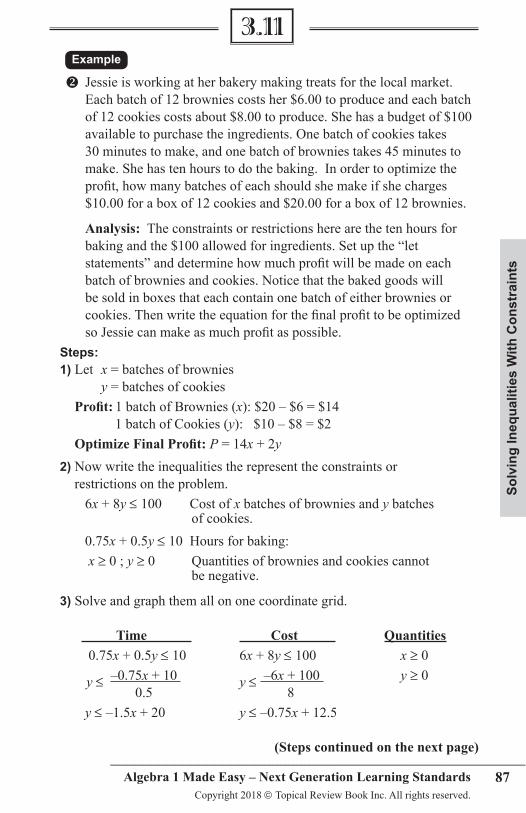
Example Jessie is working at her bakery making treats for the local market. Each batch of 12 brownies costs her $6.00 to produce and each batch of 12 cookies costs about $8.00 to produce. She has a budget of $100 available to purchase the ingredients. One batch of cookies takes 30 minutes to make, and one batch of brownies takes 45 minutes to make. She has ten hours to do the baking. In order to optimize the profit, how many batches of each should she make if she charges $10.00 for a box of 12 cookies and $20.00 for a box of 12 brownies.

Analysis: The constraints or restrictions here are the ten hours for baking and the $100 allowed for ingredients. Set up the “let statements” and determine how much profit will be made on each batch of brownies and cookies. Notice that the baked goods will be sold in boxes that each contain one batch of either brownies or cookies. Then write the equation for the final profit to be optimized so Jessie can make as much profit as possible. Steps: 1) Let x = batches of brownies y = batches of cookies Profit: 1 batch of Brownies (x): $20 – $6 = $14 1 batch of Cookies (y): $10 – $8 = $2 OptimizeFinalProfit: P = 14x + 2y 2) Now write the inequalities the represent the constraints or restrictions on the problem. 6x + 8y ≤ 100 Cost of x batches of brownies and y batches of cookies. 0.75x + 0.5y ≤ 10 Hours for baking: x ≥ 0 ; y ≥ 0 Quantities of brownies and cookies cannot be negative. 3) Solve and graph them all on one coordinate grid.

time Cost Quantities 0.75x + 0.5y ≤ 10 6x + 8y ≤ 100 x ≥ 0 y ≤ –0.75x + 10 y ≤ –6x + 100 y ≥ 0 0.5 8 y ≤ –1.5x + 20 y ≤ –0.75x + 12.5

(Steps continued on the next page)

3.11

88


onstraints


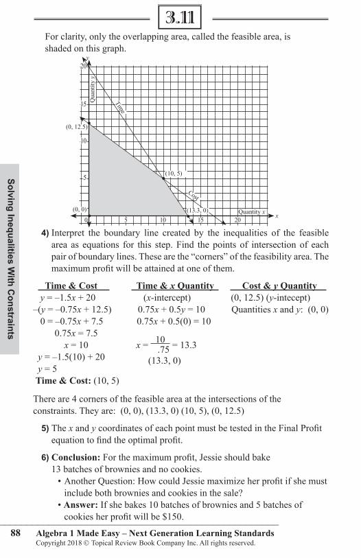
For clarity, only the overlapping area, called the feasible area, is shaded on this graph.

4) Interpret the boundary line created by the inequalities of the feasible area as equations for this step. Find the points of intersection of each pair of boundary lines. These are the “corners” of the feasibility area. The maximum profit will be attained at one of them.

time & Cost time & x Quantity Cost & y Quantity y = –1.5x + 20 (x-intercept) (0, 12.5) (y-intecept) –(y = –0.75x + 12.5) 0.75x + 0.5y = 10 Quantities x and y: (0, 0) 0 = –0.75x + 7.5 0.75x + 0.5(0) = 10 0.75x = 7.5 x = 10 x = 10 = 13.3 y = –1.5(10) + 20

.75

y = 5 (13.3, 0)

time & Cost: (10, 5)

There are 4 corners of the feasible area at the intersections of the constraints. They are: (0, 0), (13.3, 0) (10, 5), (0, 12.5)

5) The x and y coordinates of each point must be tested in the Final Profit equation to find the optimal profit. 6) Conclusion: For the maximum profit, Jessie should bake 13 batches of brownies and no cookies. • Another Question: How could Jessie maximize her profit if she must include both brownies and cookies in the sale? • Answer: If she bakes 10 batches of brownies and 5 batches of cookies her profit will be $150.

3.11

20

15

10

5

0 5 10 15 20 • •

•

(10, 5)

(0, 0) (13.3, 0)

Time

Cost

Quantity x

Qua

ntity

y

y

x

•

(0, 12.5)

1��

Types of Characteristics of D

ata


Statistics is the mathematics of collecting, organizing, summarizing, and analyzing data. The data are often displayed using graphs and tables. Data collected involve individuals which are the objects described in the data. They can be people, animals, test scores, measurements, or other items. A variableis the term used to describe the characteristic of an individual. This may have different values for different individuals. Example: If the data represent the weight of 30 dogs, each dog is an individual and the variable is the weight of the dog. If the data describe the favorite movie of each of 30 students, each student is an individual and the name of the movie is the variable.

tyPES oF VARIABLES AND DAtA

Categorical Variable: Allows the identification of the group or category in which the individual is placed.

Quantitative Variable: Results are numerical which allows arithmetic to be performed on them.

Categorical Data is non-numerical. The data values are identified by type. It is also called qualitative data.

Example Eye color, kind of pet owned, or the name of a favorite TV show or movie.

Quantitative Data is numerical. The data values (or items) are measurements or counts and have meaning as numbers.

Example Grades on a test, hours watching TV, or heights of students.

Univariate: Measurements are made on only one variable per observation.

Example • Quantitative: Ages of the students in a club. • Categorical: Kind of car owned.

Bivariate: Measurements are made on two variables per observation.

Example • Quantitative: Grade level and age of the students in a school. • Categorical: Gender and favorite T.V. shows.

DAtA 5.1

1��

Type

s &

Cha

ract

eris

tics

of D

ata



Biased: A data set that is obtained that is likely to be influenced by something – giving a “slant” to the results.

Example • Quantitative: To determine the average age of high school students by asking only tenth graders how old they are. • Categorical: Standing outside Yankee Stadium and asking people coming out of the stadium to name their favorite baseball team. Most would say … Yankees!

Unbiased: A data set that is obtained which has no connection to anything that would influence the results.

Example • Quantitative: Asking people coming out of a stadium how many pets they have. • Categorical: Asking people leaving a large grocery store what their favorite flavor of soda is.

CHARACtERIStICS oF CAtEGoRICAL AND QUANtItAtIVE DAtA

Single (ungrouped): Small samples or collections of data that can be treated as individual items. Statistical information such as mean, median, or mode, can be obtained by listing the data values individually.

Example • Quantitative: Test scores of 42, 65, 65, 70, 72, 75, 80. • Categorical: In a classroom of students what pet(s) each student has.

Grouped: When large numbers of values are included, the data are often treated in groups called intervals. The range of the data is divided into equal intervals and each item of data is recorded in the appropriate interval. The statistical information is located in the intervals.

Example • Quantitative: Heights of 200 students in a school. Their heights range, in inches, from 56″ to 75″. The intervals could be 56-60, 61-65, 66-70, 71-75. Each of the 200 students has a height within one of these intervals. • Categorical: Within certain age groups in a city, the highest level of education achieved – high school, trade school, 2 year college, 4 year college, post-graduate, doctorate.

5.1

1��

Interpreting Quantitative D

ata


RECoRDING AND ANALyZING QUANtItAtIVE DAtA

tally Sheet: A chart that is used to count the number of items with the same value (for single data items) or the items whose values fall in each interval (grouped data.) The tally sheet is marked off with small lines and every 5th tally is crossed through the previous 4 so a unit of 5 is formed.

Frequency table: A completed tally sheet which shows the intervals and the frequencies of each data item. (See page 146)

Cumulative Frequency table: Shows the sum of the frequencies at or below each of the intervals in the frequency table. The accumulation usually begins with the interval nearest zero.

QUANtItAtIVE DAtA CALCULAtIoNSUse the test scores ��, ��, ��, 70, 7�, 7�, 80

Range: Highest value in the data set minus the lowest value.

Example 80 – 42 = 38. Range = 38.

Mean: Average. The sum of the data values divided by the number of items in the data.

Example 42 + 65 + 65 + 70 + 72 + 75 + 80 = 469. Divide by 7. Mean = 67.

Mode: Value that appears most often. 65 appears twice, the mode = 65. If the data has 2 modes, it is called bimodal. Sometimes there is no mode and the data are described as having no mode.

Median: The middle data value when the data are listed in order, ascending or descending. Find the number of items, n, and divide by 2 to find the position of the middle piece of data. If n is even, find the numerical average of the values of the two middle items. In our example, n = 7. The middle item is the 4th item and its value is 70. The median = 70.

orgANiZiNg qUANtitAtive DAtA5.2

1��

Inte

rpre

ting

Qua

ntita

tive

Dat

a



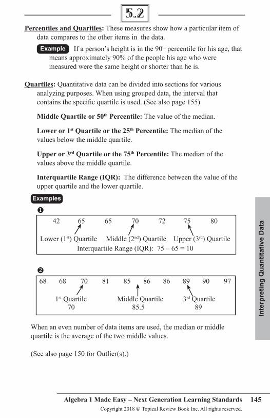
Percentiles and Quartiles: These measures show how a particular item of data compares to the other items in the data.

Example If a person’s height is in the 90th percentile for his age, that means approximately 90% of the people his age who were measured were the same height or shorter than he is.

Quartiles: Quantitative data can be divided into sections for various analyzing purposes. When using grouped data, the interval that contains the specific quartile is used. (See also page 155)

Middle Quartile or �0th Percentile: The value of the median.

Lower or 1st Quartile or the ��th Percentile: The median of the values below the middle quartile.

Upper or �rd Quartile or the 7�th Percentile: The median of the values above the middle quartile.

Interquartile Range (IQR): The difference between the value of the upper quartile and the lower quartile.

Examples

42 65 65 70 72 75 80

Lower (1st) Quartile Middle (2nd) Quartile Upper (3rd) QuartileInterquartile Range (IQR): 75 – 65 = 10

68 68 70 81 85 86 86 89 90 97

1st Quartile Middle Quartile 3rd Quartile 70 85.5 89

When an even number of data items are used, the median or middle quartile is the average of the two middle values.

(See also page 150 for Outlier(s).)

5.2

1��


ata


DISPLAyING UNIVARIAtE DAtA (oNE VARIABLE)Depending on the distribution (the way the data occur), various types of graphs are used to display the data.

Bias in Graphing: It is important when representing data on a graph to be sure the graph itself is an accurate presentation of the data. Two ways a graph can be biased are if the scales are not appropriate, or if there is a break in the presentation of the data.

Histogram: Data that are grouped in intervals are often displayed using a histogram. It is similar to a bar graph, but the “bars” are adjacent to each other and touching. The horizontal axis is labeled with the intervals; the vertical axis is the frequency, or the cumulative frequency if that is the type of histogram being used. Remember, the intervals must be of equal length, so the horizontal scale must be divided into equal segments so the “bars” are all equal in width. A histogram is not usually used for ungrouped sets of data. (See dot plots on page 157 and scatter plots on page 163.)

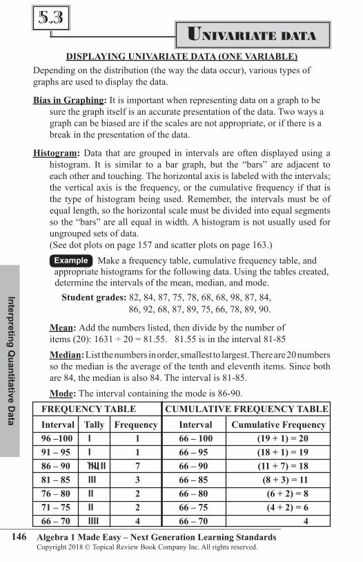
Example Make a frequency table, cumulative frequency table, and appropriate histograms for the following data. Using the tables created, determine the intervals of the mean, median, and mode. Student grades: 82, 84, 87, 75, 78, 68, 68, 98, 87, 84, 86, 92, 68, 87, 89, 75, 66, 78, 89, 90.

Mean: Add the numbers listed, then divide by the number of items (20): 1631 ÷ 20 = 81.55. 81.55 is in the interval 81-85 Median: List the numbers in order, smallest to largest. There are 20 numbers so the median is the average of the tenth and eleventh items. Since both are 84, the median is also 84. The interval is 81-85. Mode: The interval containing the mode is 86-90. FREQUENCy tABLE CUMULAtIVE FREQUENCy tABLE Interval tally Frequency Interval Cumulative Frequency 9� –100 l 1 �� – 100 (19 + 1) = �0 91 – 9� l 1 �� – 9� (18 + 1) = 19 8� – 90 l l l l ll 7 �� – 90 (11 + 7) = 18 81 – 8� lll � �� – 8� (8 + �) = 11 7� – 80 ll � �� – 80 (� + �) = 8 71 – 7� ll � �� – 7� (� + �) = � �� – 70 llll � �� – 70 �

UNivAriAte DAtA5.3

1�7

Inte

rpre

ting

Qua

ntita

tive

Dat

a



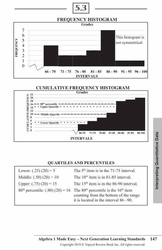
QUARtILES AND PERCENtILES

Lower: (.25) (20) = 5 The 5th item is in the 71-75 interval. Middle: (.50) (20) = 10 The 10th item is in 81-85 interval. Upper: (.75) (20) = 15 The 15th item is in the 86-90 interval. 80th percentile: (.80) (20) = 16 The 80th percentile is the 16th item counting from the bottom of the range. it is located in the interval 86 –90.

50

01234567

FR

EQ

UE

NC

Y

66 - 70 71 - 75 76 - 80 81 - 85 86 - 90 91 - 95 96 - 100

Grades

INTERVALS

FREQUENCY HISTOGRAM

MEAN: Add the numbers listed, then divide by the number of items (20): 1628 20 = is 81.4. 81.4 is in the interval 81-85

MEDIAN: List the numbers in order, smallest to largest. There are 20 numbers sothe median is the average of the tenth and eleventh items. Since both are 84, themedian is also 84. The interval is 81-85.

MODE: Look at the Frequency Histogram - the tallest bar is the interval of themode. On the frequency table, it is the interval with the highest frequency. The modeis in the interval 86-90.

QUARTILES AND PERCENTILESLower: (.25) (20) = 5 The 5th item is in the 71-75 interval.Middle: (.50) (20) = 10 The 10th item is in 81-85 interval.Upper: (.75) (20) = 15 The 15th, item is in the 86-90 interval.95th percentile: (.95) (20) = 19 The 95th percentile is at 19 which is in

the interval 91-95

CUMULATIVE FREQUENCY HISTOGRAM Grades

CU

MU

LA

TIV

E F

RE

QU

EN

CY

66-70 66-75 66-80 66-85 66-90 66-95 66-100

Lower Quartile

Upper Quartile

2220181614121086420

INTERVALS

Middle Quartile

95th percentile

• • 80th percentile • • • • • • • • • • • • • • • • • • • Upper Quartile • • • • • • • • • • • • • • • • •

• • Middle Quartile • • • • • • • • • • • • • •

• • Lower Quartile • • • • • • • •

This histogram is not symmetrical.

5.3

66-70 71-75 76-80 81-85 86-90 91-95 96-100

1�8


ata


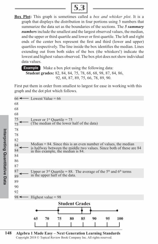
Box Plot: This graph is sometimes called a box and whisker plot. It is a graph that displays the distribution in four portions using 5 numbers that summarize the data set as the boundaries of the sections. The 5 summary numbers include the smallest and the largest observed values, the median, and the upper or third quartile and lower or first quartile. The left and right ends of the center box represent the first and third (lower and upper) quartiles respectively. The line inside the box identifies the median. Lines extending out from both sides of the box (the whiskers!) indicate the lowest and highest values observed. The box plot does not show individual data values.

Example Make a box plot using the following data: Student grades: 82, 84, 84, 75, 78, 68, 68, 98, 87, 84, 86, 92, 68, 87, 89, 75, 66, 78, 89, 90.

First put them in order from smallest to largest for ease in working with this graph and the dot plot which follows.

66 Lowest Value = 6668686875 Lower or 1st Quartile = 75 75 (The median of the lower half of the data)78788284 Median = 84. Since this is an even number of values, the median 84 is halfway between the middle two values. Since both of these are 84 84

in this example, the median is 84.

868787 Upper or 3rd Quartile = 88. The average of the 5th and 6th terms89 in the upper half of the data.89909298 Highest value = 98

Math A Made Easy Copyright Topical Review Book Inc. All rights reserved. 117

Circle Graph – (Pie Graph): A graph used to compare parts to a whole. Data isusually given in percentages. The entire circle graph represents 100%. To read acircle graph, you need to relate the percentage of each piece of data to its piece ofthe pie. Also remember that the entire circle, or 100% of the data, is 360°. Thecentral angle (shown on graph) for each section is found by multiplying 360 bythe % given.

Example: Using the test grade data above.

Letter Grade Grade Fraction Percent Central <

A 90-100 320 15% 54°

B 80-89 920 45% 162°

C 70-79 420 20% 72°

D 60-69 420 20% 72°

Test Grades

C 20%

A 15%

B 45 %

Box and Whisker Plot: Graph that shows how data is distributed.

To make a Box and Whisker Plot:

Plot the median (middle) of the data (84).

Plot the first quartile (75) and the third quartile (87) (upper and lower 25% of the data).

The “boxes” are determined by the median and quartiles.

The “whiskers” are determined by the high and low data values. 65 70 75 80 85 90 95 100

• •• • •

)

D 20%

Math A Made Easy Copyright Topical Review Book Inc. All rights reserved. 117

Circle Graph – (Pie Graph): A graph used to compare parts to a whole. Data isusually given in percentages. The entire circle graph represents 100%. To read acircle graph, you need to relate the percentage of each piece of data to its piece ofthe pie. Also remember that the entire circle, or 100% of the data, is 360°. Thecentral angle (shown on graph) for each section is found by multiplying 360 bythe % given.

Example: Using the test grade data above.

Letter Grade Grade Fraction Percent Central <

A 90-100 320 15% 54°

B 80-89 920 45% 162°

C 70-79 420 20% 72°

D 60-69 420 20% 72°

Test Grades

C 20%

A 15%

B 45 %

Box and Whisker Plot: Graph that shows how data is distributed.

To make a Box and Whisker Plot:

Plot the median (middle) of the data (84).

Plot the first quartile (75) and the third quartile (87) (upper and lower 25% of the data).

The “boxes” are determined by the median and quartiles.

The “whiskers” are determined by the high and low data values. 65 70 75 80 85 90 95 100

• •• • •

)

D 20%

Student Grades

5.3

Documents

Algebra 1 Made Easy Handbook