Algebra 2 Made Easy Handbook

Algebra 2 Made EasyHandbook

Common Core Standards Edition

By:Mary Ann Casey

B. S. Mathematics, M. S. Education

2016 Topical Review Book Company, Inc. All rights reserved.P. O. Box 328Onsted, MI. 49265-0328

This document may not, in whole or in part, be copied, photocopied, reproduced,translated, or reduced to any electronic medium or machine-readable form without prior consent in writing from Topical Review Book Corporation or its author.

AcknowledgmentsMy sincere thanks to those who helped me put Algebra II Made Easy, Common Core Edition, together. The people who contributed include Kimberly Knisell, Director of Math and Science in the Hyde Park, NY School District for her organizing expertise and to Jennifer Criser-Eighmy, Director of Humanities in Hyde Park, for proofreading the grammar and punctuation; to my daughter, Debra Rainha who teaches math at Andover (MA) High School and to her colleague, Stephanie Ragucci who teaches AP Statistics at Andover High. Her assistance was invaluable. Marin Malgieri contributed to the unit on Probability and Statistics, and additional proofreading was done by Laura Denkins. Graphics designer, Julieen Kane, at Topical Review Book Company always does a great job getting the graphs and diagrams done correctly as well as putting my drafts into the necessary form to be published. Keith Williams, owner of Topical Review Book Company, is always easy to work with and very patient. I am honored to have my work published by “the “Little Green Book” company – familiar to many for providing Regents Examination study materials since 1936.

IntroductionThis quick reference guide, or “how to do it book” It is not meant as a curriculum guide to the Common Core Standards, nor is it meant to be used as a textbook. The Common Core Standards (CCS) involve new methods of teaching and learning and use various methods for solving mathematical problems. Implementing new teaching techniques and providing deeper understanding of the content of the course is the job of the classroom teacher. As the Algebra II CCS are implemented, it is my hope that this student friendly book will assist students in becoming “college and career ready”, as this is one of the main goals of our educational process.

Sincerely,

MaryAnn Casey,B.S. Mathematics, M.S. Education

ALGEBRA 2 MADE EASYCommon Core Standards Edition

Table of Contents

UNIT 1: POLYNOMIALS, RATIONAL, AND RADICAL RELATIONSHIPS ....................................1 1.1 Real Numbers and Exponents .........................................2 1.2 Radicals ...........................................................................6 1.3 Imaginary and Complex Numbers ................................13 1.4 Factoring .......................................................................19 1.5 Polynomials ..................................................................24 1.6 Quadratic Equations ......................................................34 1.7 Rational Expressions .....................................................48 1.8 Solving Rational Equations and Inequalities ................54 1.9 Solving Radical Equations ............................................57 1.10 Systems of Equations ....................................................59 1.11 Practice and Solving Equations ....................................70 1.12 Parabola: Focus and Directrix .......................................74

UNIT 2: TRIGONOMETRY FUNCTIONS .....................................79 2.1 Arc Length ....................................................................80 2.2 Angles In Quadrants .....................................................82 2.3 Unit Circle and Trig Graphs ..........................................86 2.4 Graphing The Trig Functions ........................................89 2.5 Graphing Inverse Trig Functions ..................................99 2.6 Reciprocal Trig Functions Graphs ..............................101 2.7 Trig Identities and Equations ......................................103

UNIT 3: FUNCTIONS .....................................................................105 3.1 Functions .....................................................................106 3.2 Graphs of Functions .................................................... 112 3.3 Functions and Transformations ................................... 117 3.4 Average Rate of Change .............................................122 3.5 Inverses of Functions ..................................................124 3.6 Exponential Functions ................................................127 3.7 Logarithmic functions .................................................135 3.8 Graphing Exponential and Logarithmic Functions .....142 3.9 Polynomial Functions .................................................145 3.10 Comparing Functions ..................................................150 3.11 Sequences and Series ..................................................152

UNIT 4: PROBABILITY AND STATISTICS ...............................159 4.1 Statistics ......................................................................160 4.2 Statistical Measures ....................................................163 4.3 The Shape of a Distribution ........................................164 4.4 Inference .....................................................................170 4.5 Organizing Categorical Data .......................................173 4.6 Displaying Bivariate Data (2 Variables) .....................174 4.7 Probability ...................................................................184 4.8 Types of Probability ....................................................186 4.9 General Probability Rules ...........................................188 4.10 Independent and Conditional Events ..........................193 4.11 Probabilities Using Two-Way Table and Venn Diagrams .....................................................199

CORRELATIONS TO CCSS ...........................................................202

INDEX ................................................................................................204

ALGEBRA 2 MADE EASYCommon Core Standards Edition

Table of Contents

1Algebra 2 Made Easy – Common Core Edition Copyright 2016 Topical Review Book Company Inc. All rights reserved.

Unit 1

POLYNOMIALS, RATIONAL, AND

RADICAL RELATIONSHIPS

• Perform arithmetic operations with complex numbers.

• Use complex numbers in polynomial identities and equations.

• Interpret the structure of expressions.

• Understand the relationship between zeros and factors of polynomials.

• Use polynomial identities to solve problems.

• Rewrite rational expressions.

• Understand solving equations as a process and explain the reasoning.

• Solve equations and inequalities in one variable.

• Solve systems of equations.

• Analyze functions using different representations.

• Translate between the geometric description and the equation for a conic section.

• Extend the properties of exponents to rational exponents.

Algebra 2 Made Easy – Common Core Edition 2 Copyright 2016 Topical Review Book Company Inc. All rights reserved.

In past math courses, we have worked with the real numbers. The real numbers consist of all the numbers on the number line. In this course, we will also study numbers in the set of complex numbers.

The two main subsets of the “reals” are the rational numbers and the irrational numbers. The rational numbers include all those numbers that can be written in the form of a fraction where both the numerator and the denominator are integers. The irrational numbers include the square roots of imperfect squares, decimal numbers that do not repeat and do not terminate, Pi (π), and e which is the base of natural logarithms. (See page 143.)

A complex number can be written in the form a + bi where a and b are real numbers, i is the imaginary unit and i = -1 . (See Chapter 1.3 – Imaginary and Complex Numbers)

EXPRESSIONS WITH EXPONENTS Note: All the rules that apply to numbers with exponents are also used for expressions containing variables.

Bases and Exponents: An exponent indicates how many times to use its base as a factor. The base of the exponent is the number, variable, or parenthesis directly to the left of the exponent. If the expression to the left of the exponent is a parenthesis, the exponent is applied to the entire content of the parenthesis. Evaluating with an exponent is often referred to as “raising” a number to a power. Review of Properties of Exponents: a a a

a a

aa

a a

ab a b

ab

ab

b

a

x y x y

x y xy

x

yx y

x x x

x x

x

• =

=

= ≠

=

= ≠

+

−

( )

( )

( )

,

,

0

0

0 == ≠

= ≠−

1 0

1 01

,

,

a

aa

a

REAL NUMBERS AND EXPONENTS

1.1


The

Rea

l Num

ber S

yste

m1.1 Examples Bases and Exponents

34 = 3 • 3 • 3 • 3 = 81

–34 = – (3 • 3 • 3 • 3) = –81 ––– The base is 3. The negative sign is not directly to the left of the exponent, therefore it is not affected by the exponent.

(–3)4 = (–3)(–3)(–3)(–3) = 81 ––– Here the base is the contents of the parenthesis, –3.

5x2 = 5 • x • x = 5x2 ––– Only the x is the base for the exponent, 2.

�(5x)2 = (5x)(5x) = 25x2 ––– (5x) is directly to the left of the exponent, 2, so the entire parenthesis is the base and is multiplied by itself to evaluate the expression.

The same rule applies if the base is a fraction or a polynomial. Example

23

23

23

49

2( ) = ( ) ( ) = is different than 23

2 23

43

2= =

x (x + 2)2 = x (x + 2)(x + 2) = x3 + 4x2 + 4x, (x + 2) is the base.

Negative Exponents: A negative exponent directs us to use the reciprocal of the base raised to the indicated exponent. The negative sign has nothing to do with the positive or negative value of the base. Once we translate the base into its reciprocal, the negative sign on the exponent disappears. The positive exponent is then applied as usual.

Examples

2 12

12

12

12

18

33

− = ( ) = ( )( )( ) =

3 3 1 3 1 1 322

2( )x x x x x− = ( ) = ( )( ) =

xx x x x22 2 2 42 2

2( ) =( ) = ( )( ) =−

−( ) = −( ) = −( ) −( ) =−5 15

15

15

125

22

• •


SOLVE SYSTEMS ALGEBRAICALLYSubstitution: One equation is manipulated so that x or y is isolated, then the resulting representation of that variable is substituted in the second original equation. The remaining variable is solved for, then that answer is substituted in either original equation to find the second variable. x – y = 1 and x – 2y = 3

Steps: 1) Solve the first equation (x – y = 1) for x : x = y + 1

2) Get the second equation (x – 2y = 3) (y + 1) – 2y = 3 and substitute (y + 1) for x in it. –y + 1 = 3 Solve for y: –y = 2 y = –2 3) Go back to an original equation: x – y = 1 4) Substitute –2 for y: x – (–2) = 1 5) Solve for x: x + 2 = 1 6) Indicate both answers: x = –1 and y = –2

7) Checking both answers x – y = 1 x – 2y = 3 in both original equations –1 – (–2) = 1 –1 – 2(–2) = 3 is the final step: –1 + 2 = 1 –1 + 4 = 3 1 = 1 3 = 3

Note: This method is recommended ONLY when the coefficient of x or y is 1. Coefficients other than 1 result in fractional substitutions which must be “cleared” or they rapidly become unmanageable.

1.10


Rea

soni

ng w

ith E

quat

ions

an

d In

equa

litie

s

Addition: If two equations have the same variable with opposite coefficients, we can add the equations together and variable. Sometimes it is necessary to multiply one equation make equivalent equations that can be used in this method. Steps: 1) Arrange both equations using algebraic methods so the variables are underneath each other in position. 2) The goal is to eliminate one variable by adding the two equations together. Examine the variables and their coefficients. Find the least common multiple of the coefficients of either both x’s or both y’s. 3) Multiply each equation by a positive or negative number so the coefficients of the variable chosen are equal and opposite in sign. 4) Add the two equations together. One variable will disappear. 5) Solve for the variable that is visible. 6) Choose one of the original equations and substitute the value for the known variable to find the other variable. 7) Check in both original equations.

Example Solve the following equations for x and y: (A) 4x + 6y = 64 (B) 2x – 3y = –28Steps: 1) 6 is a common multiple for 6 and 3 so leave (A) as 2(2x – 3y = –28) ; 4x – 6y = –56 is and multiply (B) by 2.

2) Add (A) and (B) in order to isolate x: Equation (A): 4x + 6y = 64 NEW Equation (B) from step 1: 4x – 6y = –56 8x = 8 ; x = 1 3) Insert the answer back into either (A) or (B): 4(1) + 6y = 64 4) Solve for y: 6y = 60 ; y = 10 5) Check in both original equations. 4(1) + 6(10) = 64 2(1) – 3(10) = –28 64 = 64√ –28 = –28√Note: Experience will help you decide which variable to work with in the addition method. Looking for variables which already have opposite signs allows you to avoid multiplying by a negative number with its associated opportunities for error. Using small multiples is helpful, too. You wouldn’t want to use a common multiple for 11 and 14 if you could use the other variable and have a common multiple of 2 and 5.

1.10


WORD PROBLEM SYSTEMS WITH 2 VARIABLESAs in all word problems, read and reread. Make sure your equations represent the phrases in the wording of the problem. 1. Identify each unknown quantity and represent each one with a different variable in a let statement. READ CAREFULLY - make the let statement accurate. 2. Translate the verbal sentences into two equations. 3. Solve as a system of equations. Usually these problems are solved algebraically but follow directions - you might be directed to solve them graphically. 4. Check the answers in the words of the problem.

Word Problem Systems: Many word problems can be set up using two variables instead of using just one. If you choose to use that method, you must then make two equations to solve. The problem will then be solved as a “system of equations.” Example Together Evan and Denise have 28 books. If Denise has four more than Evan, how many books does each person have? Let x = the number of books Evan has Let y = the number of books Denise hasSteps: 1) Set up equation (A): x + y = 28 2) Set up equation (B): y = x + 4 3) Use substitution: x + (x + 4) = 28 2x + 4 = 28 –4 –4 4) Solve for x: 2x = 24 x = 12 x + y = 28 5) Substitute in original: 12 + x = 28 6) Solve for y: –12 –12 y = 16

Answer: Evan has 12 books and Denise has 16 books.

1.10


Rea

soni

ng w

ith E

quat

ions

an

d In

equa

litie

s

75Integrated Algebra made Easy

Copyright Topical Review Book Inc. All rights reserved.

(–1, 3)

•

• ••

•

x

y

y = –2x+ 1

y = x

+ 4

Example

Graphing Systems of linear Equations: Two or more equations are graphed on thesame coordinate plane (grid). Graph EACH equation separately but put both on one coordinate graph.

Be ACCURATE. Label each line as you graph it. The point where they intersect is the solution set of the system of equations. Label the point of intersection on the graph. This point is the solution set. Check both the x and y values of the solution in both original equations.

The x and y values of the point of intersection must satisfy both equations.

Solve this system of equations graphically and check:(A) y = x + 4 and(B) y = –2x + 1 (These are both already in y = mx + b form)

Steps: A) y = x + 4 B) y = –2x + 11) Determine the slope: slope = 1/1 slope = –2/12) Determine the y-intercept: (0, 4) (0, 1)3) Graph, label, and find solution set: SS = {(–1, 3)}4) Check: (A) y = x + 4 (B) y = –2x + 1

3 = –1 + 4 3 = –2(–1) + 1 3 = 3 3 = 2 + 1 3 = 3

5

5–5

–5

–1, 3

IAME 2009-10 MASTER.indd 75 8/5/2010 2:49:34 PM

SOLVE SYSTEMS BY GRAPHINGGraphing Systems of Linear Equations: Two or more equations are graphed on the same coordinate plane (grid). • Graph EACH equation separately, but put both on one coordinate graph. Be ACCURATE. • Label each line as you graph it. • The point where they intersect is the solution set of the system of equations. • Label the point of intersection on the graph. This point is the solution set. • Check both the x and y values of the solution in both original equations. The x and y values of the point of intersection must satisfy both equations. Example Solve this system of equations graphically and check: (A) y = x + 4 and (B) y = –2x + 1 (These are both already in y = mx + b form.)

Steps: (A) y = x + 4 (B) y = –2x + 1 1) Determine the slope: slope = 1/1 slope = –2/1 2) Determine the y-intercept: (0, 4) (0, 1) 3) Graph, label, and find solution set: SS = {(–1, 3)} 4) Check: (A) y = x + 4 (B) y = –2x + 1 3 = –1 + 4 3 = –2(–1) + 1 3 = 3√ 3 = 2 + 1 ⇒ 3 = 3√

1.10


Unit 2

TRIGONOMETRY

FUNCTIONS • Extend the domain of trigonometric functions using the unit circle.

• Model periodic phenomena with trigonometric functions.

• Prove and apply trigonometric identities.

• Summarize, represent and interpret data on two categorical and quantitative variables.


To find the length of the arc subtended (cut off by) by a central angle of a circle use this formula: s = r θ where s represents the arc length, r is the radius, and θ is the central angle MEASURED IN RADIANS. If the measure of the central angle is given in degrees, it must be changed to radian measure before using the formula.

Examples

Find the length of the arc intercepted by θ if the radius is 10 cm and θ = 2. Since θ is already in radian form, we don’t need to change it. s = r θ s = (10)(2) s = 20 cm

Find θ in radians if the arc length is 12 and the radius is 4.

s = r θ 12 = 4θ θ = 3 radians

Find the length of the arc, to the nearest tenth, cut off by a central angle measuring 75° if the radius of the circle is 5 cm. Hint: Change degrees to radians.

75180

75180

512

512

5 6 54

6 5

° •°

= =

= =

≈

( )π π π

π

radiansradians

s

s cm

( ) .

.

ARC LENGTH

2.1


Special Angles: On the unit circle, as the terminal side of θ, (in standard position), is rotated counterclockwise, the (x, y) values of each point of intersection with the unit circle are the cosine and sine values of the angle formed. Commonly, the angles that are multiples of 30°, 45°, 60° and the quadrantal angles are used to sketch the graphs of the trig functions.

θ in Radians cos θ sin θ tan θ (sin θ/cos θ) 0 * 1 0 0

6 .8660 .5 .5774

4 .7071 .7071 1

3

.5 .8660 1.7321

2

* 1 undefined 0

23

.8660 –1.7321 –.5

34

–.7071 .7071 –1

56

–.8660 .5 –.5774

π * –1 0 0

76

–.8660 –.5 .5774

54 –.7071 –.7071 1

43 –.5 –.8660 1.7321

32 * 0 –1 undefined

.5 –.8660 –1.7321

74

.7071 –.7071 –1

116

.8660 –.5 –.5774

2 π * 1 0 0 * Indicates a quadrantal angle

π

π

π

π

π

π

π

π

π

π

53

π

π

π

2.3


Trig

onom

etric

Fun

ctio

ns

Remember, a function must be one-to-one for it to have an inverse function.

To find the inverse of a function, the (x, y) coordinates of the points in the function are reversed and then they become the points on the inverse. If a point on f(x) is (2, 7), the corresponding point on f –1(x), the inverse, is (7, 2). The graph of f –1(x) is the reflection of the graph of f(x) over the line y = x.

Domain and Range of trig functions and their inverses. The domain of the function is the range of its inverse. The range of the function is the domain of its inverse. In the function, the domain shows the possible values of the angle. The range is the y values of the trig function. In the inverse, the domain is the possible values of the trig function, and the angles values are the range.

The domain of the sine, cosine, and tangent functions must be restricted.

Examples 1: :

: : 1 12 2

: 1 1 :2 2

Function sin x Inverse arc sin x or sin x

Domain x x x x

Range y y y y

f (x) = sin (x) g (x) = sin–1 (x)

–1 0 1

2

1

–1

–2

−

2

0

2

x

y

x

y

2≠4

-≠4

−

2

π

π

π

π

ππ

GRAPHING INVERSE TRIG FUNCTIONS

2.5


Unit 3

FUNCTIONS • Understand the concept of a function and use function notation.

• Interpret functions that arise in applications in terms of the context.

• Analyze functions using different representations.

• Write a function in different forms to explain different properties of the function.

• Build a function that models a relationship between two quantities.

• Build a new function from existing functions.

• Construct and compare linear, quadratic, and exponential models and solve problems.

• Interpret expressions for functions in terms of the situation they model.


Bui

ldin

g an

d In

terp

retin

g Fu

nctio

ns

Practice: Find the domain and the range where possible. It is often helpful to use a graph to find the range. Determine if the equation is a function or not, and if it is a function, is it one-to-one?

Examplesy x

x

x x

=−

−

32 7

2 7 0

2 7 72

| |

,

Domain: x x: ≠

72

Range: {y : y > 0} The graph shows the domain and range. The horizontal line test does not work so it is not one-to-one.

The vertical line test works: y

x=

-3

2 7is a function.

y x

x

x

= −

−

3 2

3 2 0

23

Domain: x x: ≥

23

Range: {y : y ≥ 0}

It passes the vertical line test and the horizontal line test. This is a one-to-one function.

y = x2 + 3x – 4 Domain: No restrictions. The domain is the set of real numbers.

Range: The minimum point on the graph of this equation is (–1.5, –6.25) The range is {y : y ≥ –6.25}

Note: Use 2nd CALC 3:minimum on the calculator. It is a function because the vertical line test works, not one-to-one.

-2

-4

-6

2

4

6

2

8

2 4 6

x

x

x

y

y

y

3.1

≠

≠ ≠

≥

≥

4

6

2

5 10-5


3.3Ef

fEc

ts o

f tr

an

sfo

rm

atio

ns

on

Pa

rEn

t fu

nc

tio

n G

ra

PHs

Pare

nt

iden

tity

(Lin

ear)

Qua

drat

ic

E

xpon

entia

l

squ

are

roo

t a

bsol

ute V

alue

func

tion

f(x

) = x

f(x

) = x

2

f(

x) =

bx ; b >

0, b

≠ 1

f(x) =

x , x

≥ 0

f(x)

= | x

|

f(x

) = m

x +

b

(

this

exam

ple,

b =

2)

Pa

rent

Gra

ph

f(x

) + a

Gra

phm

oves

up

a un

its.

f(x

) – a

Gra

phm

oves

do

wn

a un

its.

46 2 -2

x

y

2 -24 -4

x

y 2 -24 -4

x

y2 -24 -4

x

y

46 2 -2

x

y 46 2 -2

x

y

f(x) =

|x| +

2

f(x) =

|x| –

2

24

-2-4

24

-2-4

24

-2-4

24

-2-4

24

-2-4

24

-2-4

46 2 -2

x

y

24

-2-4

46 2 -2

x

y

24

-2-4

46 2 -2

x

y

24

-2-4

46 2 -2

x

y

24

-2-4

x2

4-2

46 2 -2

x

y

24

-2-4

46 2 -2

x

y

24

-2

46 2 -2

x

y

24

-2-4

f(x) =

x +

2f(x

) = x

2 + 2

f(x) =

2x +

2

f(x) =

2x –

2

f(x) =

x

+ 2

68

46 2 -2y

68

x2

4-2

f(x) =

x

– 2

46 2 -2y

68

f(x) =

x2 –

2f(x

) = x

– 2

f(

x +

a)G

raph

m

oves

L

Eft

a un

its.

f(x

– a

)G

raph

mov

es

riG

Ht

a un

its.

–f

(x)

Gra

ph is

reflected

over

the

x-ax

is.

f(

–x)

Gra

ph is

reflected

over

the

y-ax

is.

2 -24 -4

x

y

24

-2-4

2 -24 -4

x

y

24

-2-4

2 -2

x

y -2 -4

24

-2-4

46 2 -2

x

y

24

-2-4

2 -24 -4

x

y

24

-2-4

2 -24 -4

x

y

24

-2-4

46 2 -2

x

y 46 2 -2

x

y

24

-2-4

24

-2-4

46 2 -2

x

y

24

-2-4

46 2 -2

x

y

24

-2-4

-62 -2

x

y

24

-2-4

46 2 -2

x

y

24

-2-4

46 2 -2

x

y

2-2

-4

46 2 -2

x

y

24

-2-4

2 -2

x

y

24

-2-4

46 2 -2

x

y

24

-2-4

46 2 -2

x

y

2-2

-4

-4

f(x) =

(x +

2)2

-6

f(x) =

2(x –

2)

f(x) =

–(2

x )

-4 -6

f(x) =

2 – x

x2

4-2

f(x) =

x+

2

46 2 -2y

68

x2

4-2

f(x) =

x

−2

46 2 -2y

68

x2

4-2

f(x) =

–x

2 -2y

68

f(x) =

−

x

-6-8

f(x) =

(–x)

f(x) =

(–x)

2f(x

) = |–

x|

f(x) =

–|x|

f(x) =

–x2

f(x) =

–x

f(x) =

(x –

2)

f(x) =

(x –

2)2

f(x) =

|x –

2|

f(x) =

|x +

2|

f(x) =

(x +

2)

f(x) =

2(x

+ 2

)


Bui

ldin

g an

d In

terp

retin

g Fu

nctio

ns

FUNCTIONS WITH EXPONENTSExponential Function: A function with a variable in the exponent. The base of the exponent must be a positive number and not equal to 1. It is in the form: y = bx: b > 0, b ≠ 1.

The domain of an exponential function is all the real numbers. The range is y > 0.

Evaluate an Exponential Expression: If given the value of an exponent, apply it to the appropriate base and use the calculator to evaluate.

Examples Given: If x = 4, evaluate each of the following: 4x = 44 = 256

e2x = e8 = 2980.957987 (e is on the calculator)

81 81 31 1

4x = =

Solving Equations that contain a variable with a constant exponent: Remember that when raising a power to a power, the exponents are multiplied. This rule is used to solve equations where x is the base and it is raised to a constant exponent. (See Unit 1.1.) Steps: 1) Isolate the variable with its exponent. 2) Raise both sides of the equation to a power that is equal to the reciprocal of the exponent. This will make the exponent on the variable = 1. 3) Solve the remaining equation 4) Check the answers.

Examples

x Check

x

x

x

12

12

12

12

1 10

9 81 1 10

9 9 1 10

81 10 10

2

+ =

= + =

= + =

= =

:

( )

( )

( )2

3.6

EXPONENTIAL FUNCTIONS


Bui

ldin

g an

d In

terp

retin

g Fu

nctio

ns

SEQUENCESFinding a Specific Term in a Sequence

Recursive Definition or Formula: In a recursive definition or formula, the first term in a sequence is given and subsequent terms are defined by the terms before it. If an is the term we are looking for, an – 1 is the term before it. To find a specific term, terms prior to it must be found. Example Find the first 3 terms in the sequence an = 3an – 1 + 4 if a1 = 5. In this example, the first term is a1 = 5. To find the 2nd and 3rd terms, n = 2, and n = 3 need to be substituted. a1 = 5 a2 = 3(a1) + 4; a2 = 3(5) + 4; a2 = 19 a3 = 3(a2) + 4; a3 = 3(19) + 4; a3 = 61 The three terms are 5, 19, and 61. To write a recursive definition or formula when given several terms in the sequence, it is necessary to find an expression that is developed by comparing the terms and finding the process required to change each term to the subsequent term. Example Write a recursive definition for this sequence. –2, 4, 16, 256, … a1 = –2. Since 4 = (–2)2, and 16 = 42, and using the last term given to us, 256 = 162, a recursive definition for this sequence could be an = (an – 1)

2.

Explicit Formula: If specific terms are not given, a formula, sometimes called an explicit formula, is given. It can be used by substituting the number of the term desired into the formula for n. Simplify as usual.

Examples

What is the 7th term in the sequence an = 2n – 4 Since we want the 7th term, n = 7. Substitute 7 in place of n in the equation. a7 = 2(7) – 4 The 7th term in this sequence is 10. a7 = 10

What is the 5th term of the sequence an = 3n? Substitute 5 for n. a5 = 35

The 5th term in this sequence is 243. a5 = 243

What are the first 3 terms in the sequence an = n2 + 1? 3 calculations are needed: n = 1, n = 2, and n = 3. a1 = 12 + 1 = 2 a2 = 22 + 1 = 5 The first 3 terms are: 2, 5, 10 a3 = 32 + 1 = 10 Note: Terms should be in simplified whenever possible.

3.11


ARITHMETIC SEQUENCEEach term in the sequence has a common difference, d, with the term preceding it. The first term is labeled a1. The formula for finding specific terms of an arithmetic sequence is an = a1 + (n – 1)d, where an is the term desired, a1 is the first term in the sequence, n is the location in the sequence of the term desired, and d is the common difference.

• To find d, COMMON DIFFERENCE: a2 – a1 , a3 – a2 , etc. If given the first term and the value of d, the formula can be used to find other terms in the sequence.

Examples

Find the 7th term of an arithmetic sequence if a1 = 5 and d = 2. an = a1 + (n – 1)d a7 = 5 + (7 – 1)(2) a7 = 5 + 12 a7 = 17

In an arithmetic series a1 = 5. Find a10 if a6 = 17 and a7 = 19.

Find d: a7 – a6 = 19 – 17; d = 2

Use formula: an = a1 + (n – 1)d a10 = 5 + (9)(2) a10 = 23 • Recursive Formula: Terms in the sequence are given to establish a pattern. The general recursive formula for an arithmetic sequence is an = an – 1 + d but we have to find d.

Example Write the formula for this sequence. {1, 4, 7, 10, 13 …} There is a common difference, d, of 3 between each pair of consecutive terms in the sequence. Each term in the sequence is found by adding 3 to the previous term. Since the terms were given, a recursive formula can be developed. a1 = 3. an = an – 1 + 3.

Find the 6th term of this sequence: a6 = a5 + 3; a6 = 13 + 3 = 16.

The 6th term of this sequence is 16.

To find the 20th term of this sequence we would need the 19th term to use this formula. It would make more sense to use the explicit formula, an = a1 + (n – 1)d.

a20 = a1 + (20 – 1) (d); a20 = 1 + 19(3); a20 = 58

3.11


Bui

ldin

g an

d In

terp

retin

g Fu

nctio

ns

GEOMETRIC SEQUENCEThe consecutive terms are developed by multiplying each term in the sequence by a common ratio, r, to obtain the next consecutive term. The terms in the sequence have a common ratio, r a

a== 2

1. (Some texts refer to a geometric

sequence as a geometric progression.)

• To find r, the COMMON RATIO: Divide a term by the term before it. r a

a r aa== ==2

1

4

3; … Any two consecutive terms in a geometric

sequence will have the same common ratio. Examples

3, 6, 12, 24 ... Each pair of terms a1 a2 a3 a4 has a ratio of 2.

63 2 12

6 2 2412 2= = =, , .

Each term in this sequence is found by multiplying the previous term by 2.

278

94

32

94

278

23

3294

23

23, , ... ,r r= = = = =Common Ratio r

a1 a2 a3

Each term in this sequence is multiplied by 2/3 to get the next term.• Finding a Specific Term of a Geometric Sequence: Use the formula an = a1r

n – 1 where n is the index of the term desired, r is the common ratio of the sequence and a1 is the first term of the sequence. Determine the value of r first, then substitute and simplify.

Using the sequence in example 1 above, 3, 6, 12, 24, find the 12th term n = 12, r = 2, a1 = 3 a12 = a1r n – 1

a12 = (3)(2(12 – 1)) a12 = 3(2048) a12 = 6144 Find the 7th term in this sequence: 1

2

1412

12, 1

4, 1

8... First find r : r = =

a a a7

6

7 712

12

12

164

1128= • ( ) = ( ) • ( ) =; ;

The Recursive Formula for a geometric sequence is an = (an – 1)r when terms are given. Example What is the 5th term of the sequence 5, 10, 20, 40,… r r an= = = = =-

2010

2 4020

2 2 401, ; , 40 is the 4th term

a5 = (40)(2) = 80

3.11


Unit 4

PROBABILITY &

STATISTICS • Make inferences and justify conclusions from sample surveys, experiments, and observational studies.

• Understand independence and conditional probability and use them to interpret data.

• Use the rules of probability to compute probabilities of compound events in a uniform probability model.

• Summarize, represent, and interpret data on a single count or measurement variable.

• Understand and evaluated random processes underlying statistical experiments.


Statistics is a process for collecting and analyzing data in large quantities, especially for the purpose of inferring population characteristics based on a random sample from that population.

Kinds of Data Studies: The data can be collected in a variety of ways. These include:

• Population vs Sample – The type and number of people who participate in a statistical study can impact the validity of the study. Data collection that includes all members of a population, is called a census. If only part of a population is in the study it is called a sample. In a sample, the data can be expanded to include the whole group based on the expectation that the information gathered would apply to the group as a whole. We use samples to make conclusions about the entire population. The problem with samples is that they may not truly represent the population. A sample is considered random if the probability of selecting the sample is the same as the probability of selecting every other sample. When a sample is not random, a bias is introduced which may influence the study in favor of one outcome over other outcomes. A good sample must: 1. represent the whole population. 2. be large enough. 3. be randomly selected to eliminate bias.

• Survey – Used to gather large quantities of facts or opinions. Example Political parties call to ask people to name their favorite candidate.

• Observation – The observer does not have any interaction with the subjects and just examines the results of an activity. Example Count the number of people who are using a cell phone in a mall in a particular time frame. Count the number of people wearing sneakers at school.

• Controlled Experiment – Two groups are studied while an experiment is performed with one of them but not the other. Example The value of drinking orange juice to prevent a cold is measured by seeing how many people in a group given orange juice to drink for a month get a cold vs how many get a cold in the group that did not drink orange juice.

4.1

STATISTICS


Inte

rpre

ting

Cat

egor

ical

an

d Q

uant

itive

Dat

a

TYPES OF VARIABLES AND DATACategorical Variable: Allows the identification of the group or category in which the individual is placed.

Quantitative Variable: Results are numerical which allows arithmetic to be performed on them.

Categorical Data are non-numerical. The data values are identified by type. It is also called qualitative data. Example Eye color, kind of pet owned, or the name of a favorite TV show or movie.

Quantitative Data are numerical. The data values (or items) are measurements or counts and have meaning as numbers. Example Grades on a test, hours watching TV, or heights of students.

Univariate: Measurements are made on only one variable per observation. Example • Quantitative: Ages of the students in a club. • Categorical: Kind of car owned.

Bivariate: Measurements that show a relationship between two variables. Example • Quantitative: Grade level and age of the students in a school. • Categorical: Gender and favorite TV shows.

COLLECTION OF DATA Data collection must be done randomly to obtain reliable results. A sample is often used to infer the characteristics of a population.

Biased: A data set that is obtained that is likely to be influenced by something – giving a “slant” to the results. Example • Quantitative: To determine the average age of high school students by asking only tenth graders how old they are. • Categorical: Standing outside Yankee Stadium and asking people coming out of the stadium to name their favorite baseball team. Most would say … Yankees!

4.1


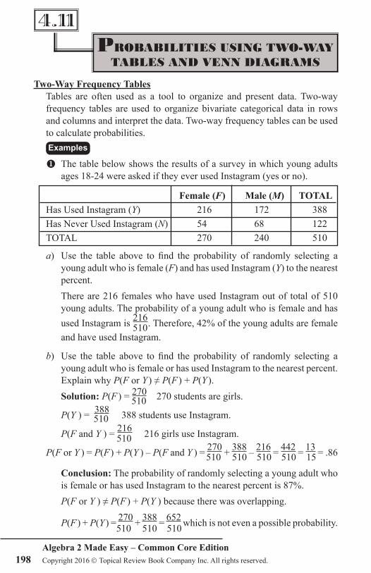
Two-Way Frequency Tables Tables are often used as a tool to organize and present data. Two-way frequency tables are used to organize bivariate categorical data in rows and columns and interpret the data. Two-way frequency tables can be used to calculate probabilities.

Examples

The table below shows the results of a survey in which young adults ages 18-24 were asked if they ever used Instagram (yes or no). Female (F) Male (M) TOTAL Has Used Instagram (Y) 216 172 388 Has Never Used Instagram (N) 54 68 122 TOTAL 270 240 510 a) Use the table above to find the probability of randomly selecting a young adult who is female (F) and has used Instagram (Y) to the nearest percent. There are 216 females who have used Instagram out of total of 510 young adults. The probability of a young adult who is female and has used Instagram is 216 . Therefore, 42% of the young adults are female 510 and have used Instagram.

b) Use the table above to find the probability of randomly selecting a young adult who is female or has used Instagram to the nearest percent. Explain why P(F or Y ) ≠ P(F ) + P(Y ). Solution: P(F ) = 270 270 students are girls. 510 P(Y ) = 388 388 students use Instagram. 510 P(F and Y ) = 216 216 girls use Instagram. 510 P(F or Y ) = P(F ) + P(Y ) – P(F and Y ) = 270 + 388 – 216 = 442 = 13 = .86 510 510 510 510 15 Conclusion: The probability of randomly selecting a young adult who is female or has used Instagram to the nearest percent is 87%. P(F or Y ) ≠ P(F ) + P(Y ) because there was overlapping.

P(F ) + P(Y ) = 270 + 388 = 652 which is not even a possible probability. 510 510 510

PROBABILITIES USING TWO-WAY TABLES AND VENN DIAGRAMS

4.11


Algebra 2 Made EasyHandbook

Common Core Standards Edition

Correlationof

Standards


CORRELATIONS TOCOMMON CORE STATE STANDARDS

Common Core State Standards Unit # . Section #

Arithmetic with Polynomials and Rational Expressions (A.APR) A.APR.4 ........................................................................................1.5 A.APR.6 .................................................................................1.5, 1.6

Creating Equations (A.CED) A.CED.1 ............................................................................... 1.6, 1.11

Reasoning with Equations and Inequalities (A.REI) A.REI.1 .........................................................................................1.6 A.REI.2 ...........................................................................1.7, 1.8, 1.9 A.REI.4 .........................................................................................1.6 A.REI.6 .......................................................................................1.10 A.REI.7 .......................................................................................1.10

Interpreting Functions (F.IF) F.IF.3 ..................................................................................... 3.5, 3.11 F.IF.4 .......................................................................................3.2, 3.3 F.IF.6 ..............................................................................................3.4 F.IF.8 .......................................................................................3.1, 3.4 F.IF.9 .......................................................................3.5, 3.6, 3.7, 3.10

Building Functions (F.BF) F.BF.1 ................................................................................... 3.9, 3.11 F.BF.2 ..........................................................................................3.10 F.BF.3 .....................................................................................3.2, 3.2 F.BF.4a ..........................................................................................3.5

Linear, Quadratic, and Exponential Models (F.LE) F.LE.2 .......................................................................................... 3.11 F.LE.4 ..............................................................................3.6, 3.7, 3.8 F.LE.5 ............................................................................................3.6


Cor

rela

tions

Trigonometric Functions (F.TF) F.TF.1 ..............................................................................2.1, 2.2, 2.3 F.TF.2 ............................................................................................2.4 F.TF.5 ..............................................................................2.4, 2.5, 2.6 F.TF.8 ............................................................................................2.7

Expressing Geometric Properties with Equations (G.GPE) G.GPE.2 ......................................................................................1.12

Making Inferences and Justifying Conclusions (S.IC) S.IC.1 .....................................................................................4.4, 4.6 S.IC.2 .....................................................................................4.4, 4.5 S.IC.3 .....................................................................................4.1, 4.6 S.IC.4 ..............................................................................4.4, 4.6, 4.8 S.IC.5 .....................................................................................4.4, 4.6 S.IC.6 .....................................................................................4.4, 4.6

Interpreting Categorical and Quantitative Data (S.ID) S.ID.4 .....................................................................................4.3, 4.4 S.ID.6 .....................................................................................4.5, 4.6

Conditional Probability and the Rules of Probability (S.CP) S.CP.1 ..............................................................................4.7, 4.8, 4.9 S.CP.2 ..........................................................................................4.10 S.CP.3 ................................................................................. 4.10, 4.11 S.CP.4 ............................................................ 4.5, 4.6, 4.9, 4.10, 4.11 S.CP.5 ................................................................................. 4.10, 4.11 S.CP.6 ..........................................................................................4.10 S.CP.7 ............................................................................................4.9

CORRELATIONS TOCOMMON CORE STATE STANDARDS

Documents

Algebra 2 Made Easy Handbook